Embed Size (px)
Citation preview
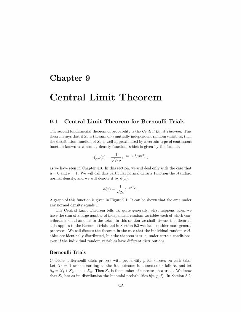
Chapter 9
Central Limit Theorem
9.1 Central Limit Theorem for Bernoulli Trials
The second fundamental theorem of probability is the Central Limit Theorem. This
theorem says that if Sn is the sum of n mutually independent random variables, then
the distribution function of Sn is well-approximated by a certain type of continuous
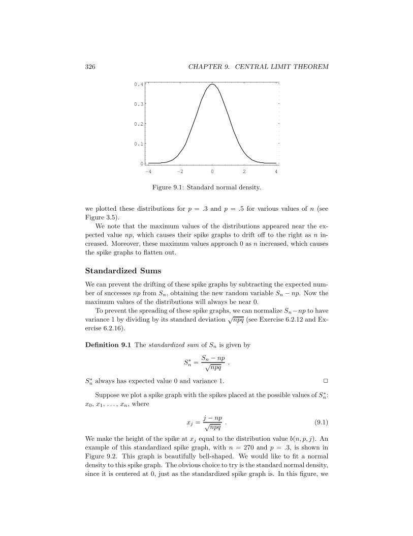
function known as a normal density function, which is given by the formula
fµ,σ(x) =1√2πσ
e−(x−µ)2/(2σ2) ,
as we have seen in Chapter 4.3. In this section, we will deal only with the case that
µ = 0 and σ = 1. We will call this particular normal density function the standard
normal density, and we will denote it by φ(x):
φ(x) =1√2π
e−x2/2 .
A graph of this function is given in Figure 9.1. It can be shown that the area under
any normal density equals 1.
The Central Limit Theorem tells us, quite generally, what happens when we
have the sum of a large number of independent random variables each of which con-
tributes a small amount to the total. In this section we shall discuss this theorem
as it applies to the Bernoulli trials and in Section 9.2 we shall consider more general
processes. We will discuss the theorem in the case that the individual random vari-
ables are identically distributed, but the theorem is true, under certain conditions,
even if the individual random variables have different distributions.
Bernoulli Trials
Consider a Bernoulli trials process with probability p for success on each trial.
Let Xi = 1 or 0 according as the ith outcome is a success or failure, and let
Sn = X1 +X2 + · · ·+Xn. Then Sn is the number of successes in n trials. We know
that Sn has as its distribution the binomial probabilities b(n, p, j). In Section 3.2,
325
326 CHAPTER 9. CENTRAL LIMIT THEOREM
-4 -2 0 2 4
0
0.1
0.2
0.3
0.4
Figure 9.1: Standard normal density.
we plotted these distributions for p = .3 and p = .5 for various values of n (see
Figure 3.5).
We note that the maximum values of the distributions appeared near the ex-
pected value np, which causes their spike graphs to drift off to the right as n in-
creased. Moreover, these maximum values approach 0 as n increased, which causes
the spike graphs to flatten out.
Standardized Sums
We can prevent the drifting of these spike graphs by subtracting the expected num-
ber of successes np from Sn, obtaining the new random variable Sn − np. Now the
maximum values of the distributions will always be near 0.
To prevent the spreading of these spike graphs, we can normalize Sn−np to have
variance 1 by dividing by its standard deviation√
npq (see Exercise 6.2.12 and Ex-
ercise 6.2.16).
Definition 9.1 The standardized sum of Sn is given by
S∗n =
Sn − np√npq
.
S∗n always has expected value 0 and variance 1. 2
Suppose we plot a spike graph with the spikes placed at the possible values of S∗n:
x0, x1, . . . , xn, where
xj =j − np√
npq. (9.1)
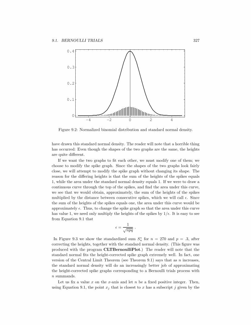
We make the height of the spike at xj equal to the distribution value b(n, p, j). An
example of this standardized spike graph, with n = 270 and p = .3, is shown in
Figure 9.2. This graph is beautifully bell-shaped. We would like to fit a normal
density to this spike graph. The obvious choice to try is the standard normal density,
since it is centered at 0, just as the standardized spike graph is. In this figure, we
9.1. BERNOULLI TRIALS 327
-4 -2 0 2 40
0.1
0.2
0.3
0.4
Figure 9.2: Normalized binomial distribution and standard normal density.
have drawn this standard normal density. The reader will note that a horrible thing
has occurred: Even though the shapes of the two graphs are the same, the heights
are quite different.
If we want the two graphs to fit each other, we must modify one of them; we
choose to modify the spike graph. Since the shapes of the two graphs look fairly
close, we will attempt to modify the spike graph without changing its shape. The
reason for the differing heights is that the sum of the heights of the spikes equals
1, while the area under the standard normal density equals 1. If we were to draw a
continuous curve through the top of the spikes, and find the area under this curve,
we see that we would obtain, approximately, the sum of the heights of the spikes
multiplied by the distance between consecutive spikes, which we will call ε. Since
the sum of the heights of the spikes equals one, the area under this curve would be
approximately ε. Thus, to change the spike graph so that the area under this curve
has value 1, we need only multiply the heights of the spikes by 1/ε. It is easy to see
from Equation 9.1 that
ε =1√npq
.
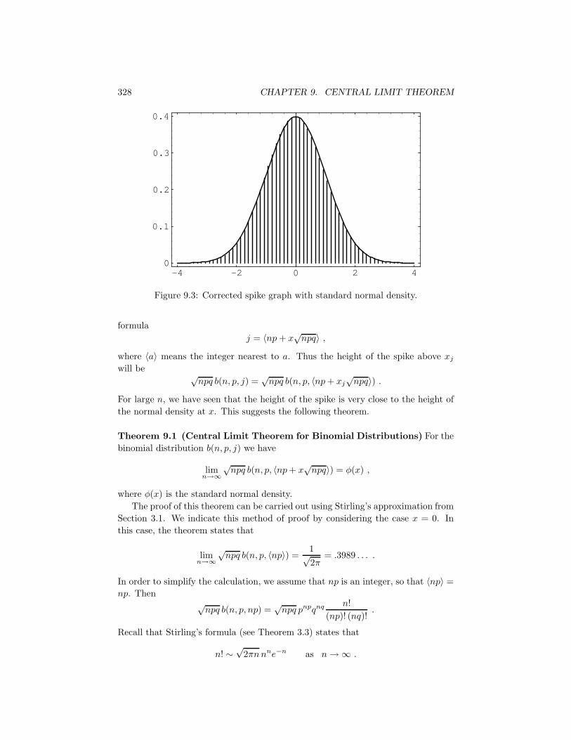
In Figure 9.3 we show the standardized sum S∗n for n = 270 and p = .3, after
correcting the heights, together with the standard normal density. (This figure was
produced with the program CLTBernoulliPlot.) The reader will note that the
standard normal fits the height-corrected spike graph extremely well. In fact, one
version of the Central Limit Theorem (see Theorem 9.1) says that as n increases,
the standard normal density will do an increasingly better job of approximating
the height-corrected spike graphs corresponding to a Bernoulli trials process with
n summands.
Let us fix a value x on the x-axis and let n be a fixed positive integer. Then,
using Equation 9.1, the point xj that is closest to x has a subscript j given by the
328 CHAPTER 9. CENTRAL LIMIT THEOREM
-4 -2 0 2 40
0.1
0.2
0.3
0.4
Figure 9.3: Corrected spike graph with standard normal density.
formula
j = 〈np + x√
npq〉 ,
where 〈a〉 means the integer nearest to a. Thus the height of the spike above xj
will be √npq b(n, p, j) =
√npq b(n, p, 〈np + xj
√npq〉) .
For large n, we have seen that the height of the spike is very close to the height of
the normal density at x. This suggests the following theorem.
Theorem 9.1 (Central Limit Theorem for Binomial Distributions) For the
binomial distribution b(n, p, j) we have
limn→∞
√npq b(n, p, 〈np + x
√npq〉) = φ(x) ,
where φ(x) is the standard normal density.
The proof of this theorem can be carried out using Stirling’s approximation from
Section 3.1. We indicate this method of proof by considering the case x = 0. In
this case, the theorem states that
limn→∞
√npq b(n, p, 〈np〉) =
1√2π
= .3989 . . . .
In order to simplify the calculation, we assume that np is an integer, so that 〈np〉 =
np. Then√
npq b(n, p, np) =√
npq pnpqnq n!
(np)! (nq)!.
Recall that Stirling’s formula (see Theorem 3.3) states that
n! ∼√
2πn nne−n as n → ∞ .
9.1. BERNOULLI TRIALS 329
Using this, we have
√npq b(n, p, np) ∼
√npq pnpqnq
√2πn nne−n
√2πnp
√2πnq (np)np(nq)nqe−npe−nq
,
which simplifies to 1/√
2π. 2
Approximating Binomial Distributions
We can use Theorem 9.1 to find approximations for the values of binomial distri-
bution functions. If we wish to find an approximation for b(n, p, j), we set
j = np + x√
npq
and solve for x, obtaining
x =j − np√
npq.
Theorem 9.1 then says that √npq b(n, p, j)
is approximately equal to φ(x), so
b(n, p, j) ≈ φ(x)√npq
=1√npq
φ
(
j − np√npq
)
.
Example 9.1 Let us estimate the probability of exactly 55 heads in 100 tosses of
a coin. For this case np = 100 · 1/2 = 50 and√
npq =√
100 · 1/2 · 1/2 = 5. Thus
x55 = (55 − 50)/5 = 1 and
P (S100 = 55) ∼ φ(1)
5=
1
5
(
1√2π
e−1/2
)
= .0484 .
To four decimal places, the actual value is .0485, and so the approximation is
very good. 2
The program CLTBernoulliLocal illustrates this approximation for any choice
of n, p, and j. We have run this program for two examples. The first is the
probability of exactly 50 heads in 100 tosses of a coin; the estimate is .0798, while the
actual value, to four decimal places, is .0796. The second example is the probability
of exactly eight sixes in 36 rolls of a die; here the estimate is .1093, while the actual
value, to four decimal places, is .1196.
330 CHAPTER 9. CENTRAL LIMIT THEOREM
The individual binomial probabilities tend to 0 as n tends to infinity. In most
applications we are not interested in the probability that a specific outcome occurs,
but rather in the probability that the outcome lies in a given interval, say the interval
[a, b]. In order to find this probability, we add the heights of the spike graphs for
values of j between a and b. This is the same as asking for the probability that the
standardized sum S∗n lies between a∗ and b∗, where a∗ and b∗ are the standardized
values of a and b. But as n tends to infinity the sum of these areas could be expected
to approach the area under the standard normal density between a∗ and b∗. The
Central Limit Theorem states that this does indeed happen.
Theorem 9.2 (Central Limit Theorem for Bernoulli Trials) Let Sn be the
number of successes in n Bernoulli trials with probability p for success, and let a
and b be two fixed real numbers. Then
limn→∞
P
(
a ≤ Sn − np√npq
≤ b
)
=
∫ b
a
φ(x) dx .
2
This theorem can be proved by adding together the approximations to b(n, p, k)
given in Theorem 9.1.It is also a special case of the more general Central Limit
Theorem (see Section 10.3).
We know from calculus that the integral on the right side of this equation is
equal to the area under the graph of the standard normal density φ(x) between
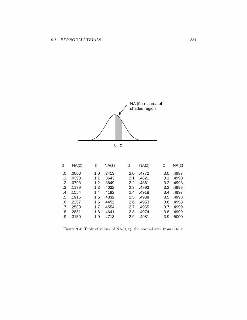
a and b. We denote this area by NA(a∗, b∗). Unfortunately, there is no simple way
to integrate the function e−x2/2, and so we must either use a table of values or else
a numerical integration program. (See Figure 9.4 for values of NA(0, z). A more
extensive table is given in Appendix A.)
It is clear from the symmetry of the standard normal density that areas such as
that between −2 and 3 can be found from this table by adding the area from 0 to 2
(same as that from −2 to 0) to the area from 0 to 3.
Approximation of Binomial Probabilities
Suppose that Sn is binomially distributed with parameters n and p. We have seen
that the above theorem shows how to estimate a probability of the form
P (i ≤ Sn ≤ j) , (9.2)
where i and j are integers between 0 and n. As we have seen, the binomial distri-
bution can be represented as a spike graph, with spikes at the integers between 0
and n, and with the height of the kth spike given by b(n, p, k). For moderate-sized
values of n, if we standardize this spike graph, and change the heights of its spikes,
in the manner described above, the sum of the heights of the spikes is approximated
by the area under the standard normal density between i∗ and j∗. It turns out that
a slightly more accurate approximation is afforded by the area under the standard
9.1. BERNOULLI TRIALS 331
NA (0,z) = area of shaded region
0 z
z NA(z) z NA(z) z NA(z) z NA(z)
.0 .0000 1.0 .3413 2.0 .4772 3.0 .4987
.1 .0398 1.1 .3643 2.1 .4821 3.1 .4990
.2 .0793 1.2 .3849 2.2 .4861 3.2 .4993
.3 .1179 1.3 .4032 2.3 .4893 3.3 .4995
.4 .1554 1.4 .4192 2.4 .4918 3.4 .4997
.5 .1915 1.5 .4332 2.5 .4938 3.5 .4998
.6 .2257 1.6 .4452 2.6 .4953 3.6 .4998
.7 .2580 1.7 .4554 2.7 .4965 3.7 .4999
.8 .2881 1.8 .4641 2.8 .4974 3.8 .4999
.9 .3159 1.9 .4713 2.9 .4981 3.9 .5000
Figure 9.4: Table of values of NA(0, z), the normal area from 0 to z.
332 CHAPTER 9. CENTRAL LIMIT THEOREM
normal density between the standardized values corresponding to (i − 1/2) and
(j + 1/2); these values are
i∗ =i − 1/2− np√
npq
and
j∗ =j + 1/2− np√
npq.
Thus,
P (i ≤ Sn ≤ j) ≈ NA
(
i − 12 − np
√npq
,j + 1
2 − np√
npq
)
.
It should be stressed that the approximations obtained by using the Central Limit
Theorem are only approximations, and sometimes they are not very close to the
actual values (see Exercise 12).
We now illustrate this idea with some examples.
Example 9.2 A coin is tossed 100 times. Estimate the probability that the number
of heads lies between 40 and 60 (the word “between” in mathematics means inclusive
of the endpoints). The expected number of heads is 100 ·1/2 = 50, and the standard
deviation for the number of heads is√
100 · 1/2 · 1/2 = 5. Thus, since n = 100 is
reasonably large, we have
P (40 ≤ Sn ≤ 60) ≈ P
(
39.5− 50
5≤ S∗
n ≤ 60.5− 50
5
)
= P (−2.1 ≤ S∗n ≤ 2.1)
≈ NA(−2.1, 2.1)
= 2NA(0, 2.1)
≈ .9642 .
The actual value is .96480, to five decimal places.
Note that in this case we are asking for the probability that the outcome will
not deviate by more than two standard deviations from the expected value. Had
we asked for the probability that the number of successes is between 35 and 65, this
would have represented three standard deviations from the mean, and, using our
1/2 correction, our estimate would be the area under the standard normal curve
between −3.1 and 3.1, or 2NA(0, 3.1) = .9980. The actual answer in this case, to
five places, is .99821. 2
It is important to work a few problems by hand to understand the conversion
from a given inequality to an inequality relating to the standardized variable. After
this, one can then use a computer program that carries out this conversion, including
the 1/2 correction. The program CLTBernoulliGlobal is such a program for
estimating probabilities of the form P (a ≤ Sn ≤ b).
Example 9.3 Dartmouth College would like to have 1050 freshmen. This college
cannot accommodate more than 1060. Assume that each applicant accepts with
9.1. BERNOULLI TRIALS 333
probability .6 and that the acceptances can be modeled by Bernoulli trials. If the
college accepts 1700, what is the probability that it will have too many acceptances?
If it accepts 1700 students, the expected number of students who matricu-
late is .6 · 1700 = 1020. The standard deviation for the number that accept is√1700 · .6 · .4 ≈ 20. Thus we want to estimate the probability
P (S1700 > 1060) = P (S1700 ≥ 1061)
= P
(
S∗1700 ≥ 1060.5− 1020
20
)
= P (S∗1700 ≥ 2.025) .
From Table 9.4, if we interpolate, we would estimate this probability to be
.5 − .4784 = .0216. Thus, the college is fairly safe using this admission policy. 2
Applications to Statistics
There are many important questions in the field of statistics that can be answered
using the Central Limit Theorem for independent trials processes. The following
example is one that is encountered quite frequently in the news. Another example
of an application of the Central Limit Theorem to statistics is given in Section 9.2.
Example 9.4 One frequently reads that a poll has been taken to estimate the pro-
portion of people in a certain population who favor one candidate over another in
a race with two candidates. (This model also applies to races with more than two
candidates A and B, and two ballot propositions.) Clearly, it is not possible for
pollsters to ask everyone for their preference. What is done instead is to pick a
subset of the population, called a sample, and ask everyone in the sample for their
preference. Let p be the actual proportion of people in the population who are in
favor of candidate A and let q = 1−p. If we choose a sample of size n from the pop-
ulation, the preferences of the people in the sample can be represented by random
variables X1, X2, . . . , Xn, where Xi = 1 if person i is in favor of candidate A, and
Xi = 0 if person i is in favor of candidate B. Let Sn = X1 + X2 + · · ·+ Xn. If each
subset of size n is chosen with the same probability, then Sn is hypergeometrically
distributed. If n is small relative to the size of the population (which is typically
true in practice), then Sn is approximately binomially distributed, with parameters
n and p.
The pollster wants to estimate the value p. An estimate for p is provided by the
value p̄ = Sn/n, which is the proportion of people in the sample who favor candidate
B. The Central Limit Theorem says that the random variable p̄ is approximately
normally distributed. (In fact, our version of the Central Limit Theorem says that
the distribution function of the random variable
S∗n =
Sn − np√npq
is approximated by the standard normal density.) But we have
p̄ =Sn − np√
npq
√
pq
n+ p ,
334 CHAPTER 9. CENTRAL LIMIT THEOREM
i.e., p̄ is just a linear function of S∗n. Since the distribution of S∗
n is approximated
by the standard normal density, the distribution of the random variable p̄ must also
be bell-shaped. We also know how to write the mean and standard deviation of p̄
in terms of p and n. The mean of p̄ is just p, and the standard deviation is
√
pq
n.
Thus, it is easy to write down the standardized version of p̄; it is
p̄∗ =p̄ − p√
pq/n.
Since the distribution of the standardized version of p̄ is approximated by the
standard normal density, we know, for example, that 95% of its values will lie within
two standard deviations of its mean, and the same is true of p̄. So we have
P
(
p − 2
√
pq
n< p̄ < p + 2
√
pq
n
)
≈ .954 .
Now the pollster does not know p or q, but he can use p̄ and q̄ = 1 − p̄ in their
place without too much danger. With this idea in mind, the above statement is
equivalent to the statement
P
(
p̄ − 2
√
p̄q̄
n< p < p̄ + 2
√
p̄q̄
n
)
≈ .954 .
The resulting interval(
p̄ − 2√
p̄q̄√n
, p̄ +2√
p̄q̄√n
)
is called the 95 percent confidence interval for the unknown value of p. The name
is suggested by the fact that if we use this method to estimate p in a large number
of samples we should expect that in about 95 percent of the samples the true value
of p is contained in the confidence interval obtained from the sample. In Exercise 11
you are asked to write a program to illustrate that this does indeed happen.
The pollster has control over the value of n. Thus, if he wants to create a 95%
confidence interval with length 6%, then he should choose a value of n so that
2√
p̄q̄√n
≤ .03 .
Using the fact that p̄q̄ ≤ 1/4, no matter what the value of p̄ is, it is easy to show
that if he chooses a value of n so that
1√n≤ .03 ,
he will be safe. This is equivalent to choosing
n ≥ 1111 .
9.1. BERNOULLI TRIALS 335
0.48 0.5 0.52 0.54 0.56 0.58 0.6
0
5
10
15
20
25
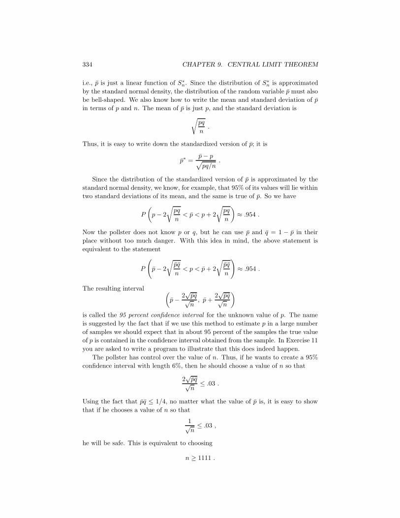
Figure 9.5: Polling simulation.
So if the pollster chooses n to be 1200, say, and calculates p̄ using his sample of size
1200, then 19 times out of 20 (i.e., 95% of the time), his confidence interval, which
is of length 6%, will contain the true value of p. This type of confidence interval
is typically reported in the news as follows: this survey has a 3% margin of error.
In fact, most of the surveys that one sees reported in the paper will have sample
sizes around 1000. A somewhat surprising fact is that the size of the population has
apparently no effect on the sample size needed to obtain a 95% confidence interval
for p with a given margin of error. To see this, note that the value of n that was
needed depended only on the number .03, which is the margin of error. In other
words, whether the population is of size 100,000 or 100,000,000, the pollster needs
only to choose a sample of size 1200 or so to get the same accuracy of estimate of
p. (We did use the fact that the sample size was small relative to the population
size in the statement that Sn is approximately binomially distributed.)
In Figure 9.5, we show the results of simulating the polling process. The popula-
tion is of size 100,000, and for the population, p = .54. The sample size was chosen
to be 1200. The spike graph shows the distribution of p̄ for 10,000 randomly chosen
samples. For this simulation, the program kept track of the number of samples for
which p̄ was within 3% of .54. This number was 9648, which is close to 95% of the
number of samples used.
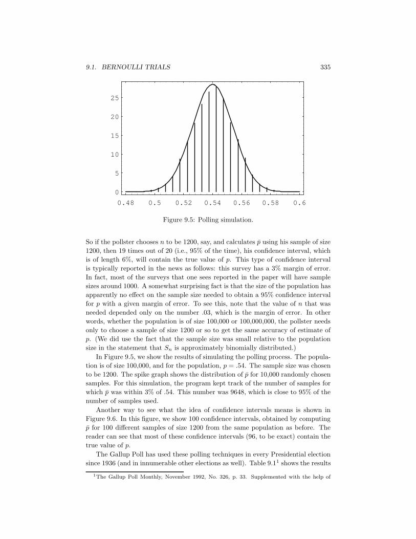
Another way to see what the idea of confidence intervals means is shown in
Figure 9.6. In this figure, we show 100 confidence intervals, obtained by computing
p̄ for 100 different samples of size 1200 from the same population as before. The
reader can see that most of these confidence intervals (96, to be exact) contain the
true value of p.
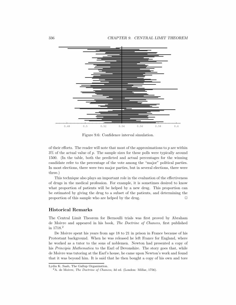
The Gallup Poll has used these polling techniques in every Presidential election
since 1936 (and in innumerable other elections as well). Table 9.11 shows the results
1The Gallup Poll Monthly, November 1992, No. 326, p. 33. Supplemented with the help of
336 CHAPTER 9. CENTRAL LIMIT THEOREM
0.48 0.5 0.52 0.54 0.56 0.58 0.6
Figure 9.6: Confidence interval simulation.
of their efforts. The reader will note that most of the approximations to p are within
3% of the actual value of p. The sample sizes for these polls were typically around
1500. (In the table, both the predicted and actual percentages for the winning
candidate refer to the percentage of the vote among the “major” political parties.
In most elections, there were two major parties, but in several elections, there were
three.)
This technique also plays an important role in the evaluation of the effectiveness
of drugs in the medical profession. For example, it is sometimes desired to know
what proportion of patients will be helped by a new drug. This proportion can
be estimated by giving the drug to a subset of the patients, and determining the
proportion of this sample who are helped by the drug. 2
Historical Remarks
The Central Limit Theorem for Bernoulli trials was first proved by Abraham
de Moivre and appeared in his book, The Doctrine of Chances, first published
in 1718.2
De Moivre spent his years from age 18 to 21 in prison in France because of his
Protestant background. When he was released he left France for England, where
he worked as a tutor to the sons of noblemen. Newton had presented a copy of
his Principia Mathematica to the Earl of Devonshire. The story goes that, while
de Moivre was tutoring at the Earl’s house, he came upon Newton’s work and found
that it was beyond him. It is said that he then bought a copy of his own and tore
Lydia K. Saab, The Gallup Organization.2A. de Moivre, The Doctrine of Chances, 3d ed. (London: Millar, 1756).
9.1. BERNOULLI TRIALS 337
Year Winning Gallup Final Election DeviationCandidate Survey Result
1936 Roosevelt 55.7% 62.5% 6.8%1940 Roosevelt 52.0% 55.0% 3.0%1944 Roosevelt 51.5% 53.3% 1.8%1948 Truman 44.5% 49.9% 5.4%1952 Eisenhower 51.0% 55.4% 4.4%1956 Eisenhower 59.5% 57.8% 1.7%1960 Kennedy 51.0% 50.1% 0.9%1964 Johnson 64.0% 61.3% 2.7%1968 Nixon 43.0% 43.5% 0.5%1972 Nixon 62.0% 61.8% 0.2%1976 Carter 48.0% 50.0% 2.0%1980 Reagan 47.0% 50.8% 3.8%1984 Reagan 59.0% 59.1% 0.1%1988 Bush 56.0% 53.9% 2.1%1992 Clinton 49.0% 43.2% 5.8%1996 Clinton 52.0% 50.1% 1.9%
Table 9.1: Gallup Poll accuracy record.
it into separate pages, learning it page by page as he walked around London to his
tutoring jobs. De Moivre frequented the coffeehouses in London, where he started
his probability work by calculating odds for gamblers. He also met Newton at such a
coffeehouse and they became fast friends. De Moivre dedicated his book to Newton.
The Doctrine of Chances provides the techniques for solving a wide variety of
gambling problems. In the midst of these gambling problems de Moivre rather
modestly introduces his proof of the Central Limit Theorem, writing
A Method of approximating the Sum of the Terms of the Binomial
(a + b)n expanded into a Series, from whence are deduced some prac-
tical Rules to estimate the Degree of Assent which is to be given to
Experiments.3
De Moivre’s proof used the approximation to factorials that we now call Stirling’s
formula. De Moivre states that he had obtained this formula before Stirling but
without determining the exact value of the constant√
2π. While he says it is not
really necessary to know this exact value, he concedes that knowing it “has spread
a singular Elegancy on the Solution.”
The complete proof and an interesting discussion of the life of de Moivre can be
found in the book Games, Gods and Gambling by F. N. David.4
3ibid., p. 243.4F. N. David, Games, Gods and Gambling (London: Griffin, 1962).
338 CHAPTER 9. CENTRAL LIMIT THEOREM
Exercises
1 Let S100 be the number of heads that turn up in 100 tosses of a fair coin. Use
the Central Limit Theorem to estimate
(a) P (S100 ≤ 45).
(b) P (45 < S100 < 55).
(c) P (S100 > 63).
(d) P (S100 < 57).
2 Let S200 be the number of heads that turn up in 200 tosses of a fair coin.
Estimate
(a) P (S200 = 100).
(b) P (S200 = 90).
(c) P (S200 = 80).
3 A true-false examination has 48 questions. June has probability 3/4 of an-
swering a question correctly. April just guesses on each question. A passing
score is 30 or more correct answers. Compare the probability that June passes
the exam with the probability that April passes it.
4 Let S be the number of heads in 1,000,000 tosses of a fair coin. Use (a) Cheby-
shev’s inequality, and (b) the Central Limit Theorem, to estimate the prob-
ability that S lies between 499,500 and 500,500. Use the same two methods
to estimate the probability that S lies between 499,000 and 501,000, and the
probability that S lies between 498,500 and 501,500.
5 A rookie is brought to a baseball club on the assumption that he will have a
.300 batting average. (Batting average is the ratio of the number of hits to the
number of times at bat.) In the first year, he comes to bat 300 times and his
batting average is .267. Assume that his at bats can be considered Bernoulli
trials with probability .3 for success. Could such a low average be considered
just bad luck or should he be sent back to the minor leagues? Comment on
the assumption of Bernoulli trials in this situation.
6 Once upon a time, there were two railway trains competing for the passenger
traffic of 1000 people leaving from Chicago at the same hour and going to Los
Angeles. Assume that passengers are equally likely to choose each train. How
many seats must a train have to assure a probability of .99 or better of having
a seat for each passenger?
7 Assume that, as in Example 9.3, Dartmouth admits 1750 students. What is
the probability of too many acceptances?
8 A club serves dinner to members only. They are seated at 12-seat tables. The
manager observes over a long period of time that 95 percent of the time there
are between six and nine full tables of members, and the remainder of the
9.1. BERNOULLI TRIALS 339
time the numbers are equally likely to fall above or below this range. Assume
that each member decides to come with a given probability p, and that the
decisions are independent. How many members are there? What is p?
9 Let Sn be the number of successes in n Bernoulli trials with probability .8 for
success on each trial. Let An = Sn/n be the average number of successes. In
each case give the value for the limit, and give a reason for your answer.
(a) limn→∞ P (An = .8).
(b) limn→∞ P (.7n < Sn < .9n).
(c) limn→∞ P (Sn < .8n + .8√
n).
(d) limn→∞ P (.79 < An < .81).
10 Find the probability that among 10,000 random digits the digit 3 appears not
more than 931 times.
11 Write a computer program to simulate 10,000 Bernoulli trials with probabil-
ity .3 for success on each trial. Have the program compute the 95 percent
confidence interval for the probability of success based on the proportion of
successes. Repeat the experiment 100 times and see how many times the true
value of .3 is included within the confidence limits.
12 A balanced coin is flipped 400 times. Determine the number x such that
the probability that the number of heads is between 200 − x and 200 + x is
approximately .80.
13 A noodle machine in Spumoni’s spaghetti factory makes about 5 percent de-
fective noodles even when properly adjusted. The noodles are then packed
in crates containing 1900 noodles each. A crate is examined and found to
contain 115 defective noodles. What is the approximate probability of finding
at least this many defective noodles if the machine is properly adjusted?
14 A restaurant feeds 400 customers per day. On the average 20 percent of the
customers order apple pie.
(a) Give a range (called a 95 percent confidence interval) for the number of
pieces of apple pie ordered on a given day such that you can be 95 percent
sure that the actual number will fall in this range.
(b) How many customers must the restaurant have, on the average, to be at
least 95 percent sure that the number of customers ordering pie on that
day falls in the 19 to 21 percent range?
15 Recall that if X is a random variable, the cumulative distribution function
of X is the function F (x) defined by
F (x) = P (X ≤ x) .
(a) Let Sn be the number of successes in n Bernoulli trials with probability p
for success. Write a program to plot the cumulative distribution for Sn.
340 CHAPTER 9. CENTRAL LIMIT THEOREM
(b) Modify your program in (a) to plot the cumulative distribution F ∗n(x) of
the standardized random variable
S∗n =
Sn − np√npq
.
(c) Define the normal distribution N(x) to be the area under the normal
curve up to the value x. Modify your program in (b) to plot the normal
distribution as well, and compare it with the cumulative distribution
of S∗n. Do this for n = 10, 50, and 100.
16 In Example 3.11, we were interested in testing the hypothesis that a new form
of aspirin is effective 80 percent of the time rather than the 60 percent of the
time as reported for standard aspirin. The new aspirin is given to n people.
If it is effective in m or more cases, we accept the claim that the new drug
is effective 80 percent of the time and if not we reject the claim. Using the
Central Limit Theorem, show that you can choose the number of trials n and
the critical value m so that the probability that we reject the hypothesis when
it is true is less than .01 and the probability that we accept it when it is false
is also less than .01. Find the smallest value of n that will suffice for this.
17 In an opinion poll it is assumed that an unknown proportion p of the people
are in favor of a proposed new law and a proportion 1 − p are against it.
A sample of n people is taken to obtain their opinion. The proportion p̄ in
favor in the sample is taken as an estimate of p. Using the Central Limit
Theorem, determine how large a sample will ensure that the estimate will,
with probability .95, be correct to within .01.
18 A description of a poll in a certain newspaper says that one can be 95%
confident that error due to sampling will be no more than plus or minus 3
percentage points. A poll in the New York Times taken in Iowa says that
“according to statistical theory, in 19 out of 20 cases the results based on such
samples will differ by no more than 3 percentage points in either direction
from what would have been obtained by interviewing all adult Iowans.” These
are both attempts to explain the concept of confidence intervals. Do both
statements say the same thing? If not, which do you think is the more accurate
description?
9.2 Central Limit Theorem for Discrete Indepen-
dent Trials
We have illustrated the Central Limit Theorem in the case of Bernoulli trials, but
this theorem applies to a much more general class of chance processes. In particular,
it applies to any independent trials process such that the individual trials have finite
variance. For such a process, both the normal approximation for individual terms
and the Central Limit Theorem are valid.
9.2. DISCRETE INDEPENDENT TRIALS 341
Let Sn = X1 + X2 + · · · + Xn be the sum of n independent discrete random
variables of an independent trials process with common distribution function m(x)
defined on the integers, with mean µ and variance σ2. We have seen in Section 7.2
that the distributions for such independent sums have shapes resembling the nor-
mal curve, but the largest values drift to the right and the curves flatten out (see
Figure 7.6). We can prevent this just as we did for Bernoulli trials.
Standardized Sums
Consider the standardized random variable
S∗n =
Sn − nµ√nσ2
.
This standardizes Sn to have expected value 0 and variance 1. If Sn = j, then
S∗n has the value xj with
xj =j − nµ√
nσ2.
We can construct a spike graph just as we did for Bernoulli trials. Each spike is
centered at some xj . The distance between successive spikes is
b =1√nσ2
,
and the height of the spike is
h =√
nσ2P (Sn = j) .
The case of Bernoulli trials is the special case for which Xj = 1 if the jth
outcome is a success and 0 otherwise; then µ = p and σ2 =√
pq.
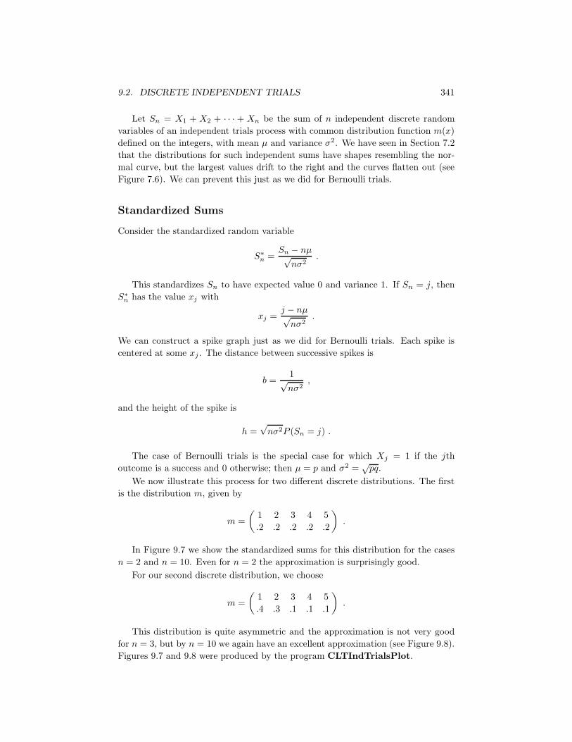
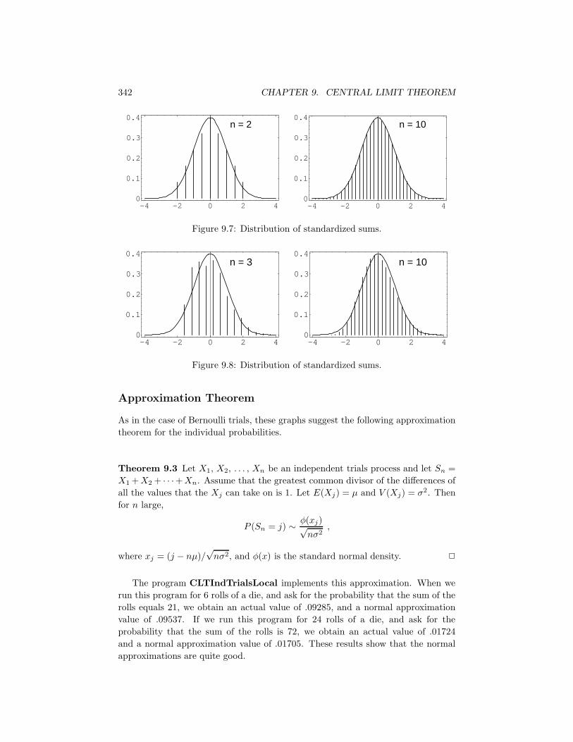
We now illustrate this process for two different discrete distributions. The first
is the distribution m, given by
m =
(
1 2 3 4 5
.2 .2 .2 .2 .2
)
.
In Figure 9.7 we show the standardized sums for this distribution for the cases
n = 2 and n = 10. Even for n = 2 the approximation is surprisingly good.
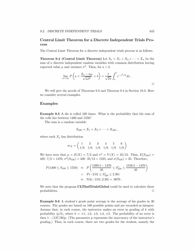
For our second discrete distribution, we choose
m =
(
1 2 3 4 5
.4 .3 .1 .1 .1
)
.
This distribution is quite asymmetric and the approximation is not very good
for n = 3, but by n = 10 we again have an excellent approximation (see Figure 9.8).
Figures 9.7 and 9.8 were produced by the program CLTIndTrialsPlot.
342 CHAPTER 9. CENTRAL LIMIT THEOREM
-4 -2 0 2 40
0.1
0.2
0.3
0.4
-4 -2 0 2 40
0.1
0.2
0.3
0.4n = 2 n = 10
Figure 9.7: Distribution of standardized sums.
-4 -2 0 2 40
0.1
0.2
0.3
0.4
-4 -2 0 2 40
0.1
0.2
0.3
0.4n = 3 n = 10
Figure 9.8: Distribution of standardized sums.
Approximation Theorem
As in the case of Bernoulli trials, these graphs suggest the following approximation
theorem for the individual probabilities.
Theorem 9.3 Let X1, X2, . . . , Xn be an independent trials process and let Sn =
X1 + X2 + · · ·+ Xn. Assume that the greatest common divisor of the differences of
all the values that the Xj can take on is 1. Let E(Xj) = µ and V (Xj) = σ2. Then
for n large,
P (Sn = j) ∼ φ(xj)√nσ2
,
where xj = (j − nµ)/√
nσ2, and φ(x) is the standard normal density. 2
The program CLTIndTrialsLocal implements this approximation. When we
run this program for 6 rolls of a die, and ask for the probability that the sum of the
rolls equals 21, we obtain an actual value of .09285, and a normal approximation
value of .09537. If we run this program for 24 rolls of a die, and ask for the
probability that the sum of the rolls is 72, we obtain an actual value of .01724
and a normal approximation value of .01705. These results show that the normal
approximations are quite good.
9.2. DISCRETE INDEPENDENT TRIALS 343
Central Limit Theorem for a Discrete Independent Trials Pro-
cess
The Central Limit Theorem for a discrete independent trials process is as follows.
Theorem 9.4 (Central Limit Theorem) Let Sn = X1 + X2 + · · · + Xn be the
sum of n discrete independent random variables with common distribution having
expected value µ and variance σ2. Then, for a < b,
limn→∞
P
(
a <Sn − nµ√
nσ2< b
)
=1√2π
∫ b
a
e−x2/2 dx .
2
We will give the proofs of Theorems 9.3 and Theorem 9.4 in Section 10.3. Here
we consider several examples.
Examples
Example 9.5 A die is rolled 420 times. What is the probability that the sum of
the rolls lies between 1400 and 1550?
The sum is a random variable
S420 = X1 + X2 + · · · + X420 ,
where each Xj has distribution
mX =
(
1 2 3 4 5 6
1/6 1/6 1/6 1/6 1/6 1/6
)
We have seen that µ = E(X) = 7/2 and σ2 = V (X) = 35/12. Thus, E(S420) =
420 · 7/2 = 1470, σ2(S420) = 420 · 35/12 = 1225, and σ(S420) = 35. Therefore,
P (1400 ≤ S420 ≤ 1550) ≈ P
(
1399.5− 1470
35≤ S∗
420 ≤ 1550.5− 1470
35
)
= P (−2.01 ≤ S∗420 ≤ 2.30)
≈ NA(−2.01, 2.30) = .9670 .
We note that the program CLTIndTrialsGlobal could be used to calculate these
probabilities. 2
Example 9.6 A student’s grade point average is the average of his grades in 30
courses. The grades are based on 100 possible points and are recorded as integers.
Assume that, in each course, the instructor makes an error in grading of k with
probability |p/k|, where k = ±1, ±2, ±3, ±4, ±5. The probability of no error is
then 1− (137/30)p. (The parameter p represents the inaccuracy of the instructor’s
grading.) Thus, in each course, there are two grades for the student, namely the
344 CHAPTER 9. CENTRAL LIMIT THEOREM
“correct” grade and the recorded grade. So there are two average grades for the
student, namely the average of the correct grades and the average of the recorded
grades.
We wish to estimate the probability that these two average grades differ by less
than .05 for a given student. We now assume that p = 1/20. We also assume
that the total error is the sum S30 of 30 independent random variables each with
distribution
mX :
{
−5 −4 −3 −2 −1 0 1 2 3 4 51
100180
160
140
120
463600
120
140
160
180
1100
}
.
One can easily calculate that E(X) = 0 and σ2(X) = 1.5. Then we have
P(
−.05 ≤ S30
30 ≤ .05)
= P (−1.5 ≤ S30 ≤ 1.5)
= P(
−1.5√30·1.5
≤ S∗30 ≤ 1.5√
30·1.5
)
= P (−.224 ≤ S∗30 ≤ .224)
≈ NA(−.224, .224) = .1772 .
This means that there is only a 17.7% chance that a given student’s grade point
average is accurate to within .05. (Thus, for example, if two candidates for valedic-
torian have recorded averages of 97.1 and 97.2, there is an appreciable probability
that their correct averages are in the reverse order.) For a further discussion of this
example, see the article by R. M. Kozelka.5 2
A More General Central Limit Theorem
In Theorem 9.4, the discrete random variables that were being summed were as-
sumed to be independent and identically distributed. It turns out that the assump-
tion of identical distributions can be substantially weakened. Much work has been
done in this area, with an important contribution being made by J. W. Lindeberg.
Lindeberg found a condition on the sequence {Xn} which guarantees that the dis-
tribution of the sum Sn is asymptotically normally distributed. Feller showed that
Lindeberg’s condition is necessary as well, in the sense that if the condition does
not hold, then the sum Sn is not asymptotically normally distributed. For a pre-
cise statement of Lindeberg’s Theorem, we refer the reader to Feller.6 A sufficient
condition that is stronger (but easier to state) than Lindeberg’s condition, and is
weaker than the condition in Theorem 9.4, is given in the following theorem.
5R. M. Kozelka, “Grade-Point Averages and the Central Limit Theorem,” American Math.
Monthly, vol. 86 (Nov 1979), pp. 773-777.6W. Feller, Introduction to Probability Theory and its Applications, vol. 1, 3rd ed. (New York:
John Wiley & Sons, 1968), p. 254.
9.2. DISCRETE INDEPENDENT TRIALS 345
Theorem 9.5 (Central Limit Theorem) Let X1, X2, . . . , Xn , . . . be a se-
quence of independent discrete random variables, and let Sn = X1 +X2 + · · ·+Xn.
For each n, denote the mean and variance of Xn by µn and σ2n, respectively. De-
fine the mean and variance of Sn to be mn and s2n, respectively, and assume that
sn → ∞. If there exists a constant A, such that |Xn| ≤ A for all n, then for a < b,
limn→∞
P
(
a <Sn − mn
sn< b
)
=1√2π
∫ b
a
e−x2/2 dx .
2
The condition that |Xn| ≤ A for all n is sometimes described by saying that the
sequence {Xn} is uniformly bounded. The condition that sn → ∞ is necessary (see
Exercise 15).
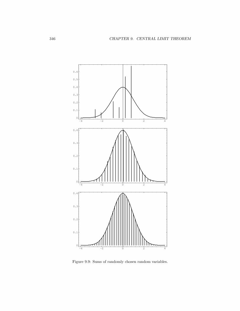
We illustrate this theorem by generating a sequence of n random distributions on
the interval [a, b]. We then convolute these distributions to find the distribution of
the sum of n independent experiments governed by these distributions. Finally, we
standardize the distribution for the sum to have mean 0 and standard deviation 1
and compare it with the normal density. The program CLTGeneral carries out
this procedure.
In Figure 9.9 we show the result of running this program for [a, b] = [−2, 4], and
n = 1, 4, and 10. We see that our first random distribution is quite asymmetric.
By the time we choose the sum of ten such experiments we have a very good fit to
the normal curve.
The above theorem essentially says that anything that can be thought of as being
made up as the sum of many small independent pieces is approximately normally
distributed. This brings us to one of the most important questions that was asked
about genetics in the 1800’s.
The Normal Distribution and Genetics
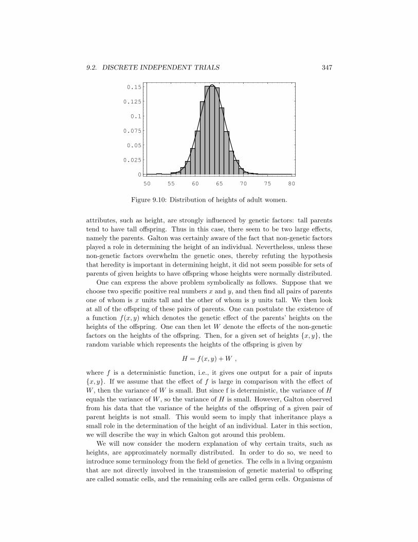
When one looks at the distribution of heights of adults of one sex in a given pop-
ulation, one cannot help but notice that this distribution looks like the normal
distribution. An example of this is shown in Figure 9.10. This figure shows the
distribution of heights of 9593 women between the ages of 21 and 74. These data
come from the Health and Nutrition Examination Survey I (HANES I). For this
survey, a sample of the U.S. civilian population was chosen. The survey was carried
out between 1971 and 1974.
A natural question to ask is “How does this come about?”. Francis Galton,
an English scientist in the 19th century, studied this question, and other related
questions, and constructed probability models that were of great importance in
explaining the genetic effects on such attributes as height. In fact, one of the most
important ideas in statistics, the idea of regression to the mean, was invented by
Galton in his attempts to understand these genetic effects.
Galton was faced with an apparent contradiction. On the one hand, he knew
that the normal distribution arises in situations in which many small independent
effects are being summed. On the other hand, he also knew that many quantitative
346 CHAPTER 9. CENTRAL LIMIT THEOREM
-4 -2 0 2 40
0.1
0.2
0.3
0.4
0.5
0.6
-4 -2 0 2 40
0.1
0.2
0.3
0.4
-4 -2 0 2 40
0.1
0.2
0.3
0.4
Figure 9.9: Sums of randomly chosen random variables.
9.2. DISCRETE INDEPENDENT TRIALS 347
50 55 60 65 70 75 80
0
0.025
0.05
0.075
0.1
0.125
0.15
Figure 9.10: Distribution of heights of adult women.
attributes, such as height, are strongly influenced by genetic factors: tall parents
tend to have tall offspring. Thus in this case, there seem to be two large effects,
namely the parents. Galton was certainly aware of the fact that non-genetic factors
played a role in determining the height of an individual. Nevertheless, unless these
non-genetic factors overwhelm the genetic ones, thereby refuting the hypothesis
that heredity is important in determining height, it did not seem possible for sets of
parents of given heights to have offspring whose heights were normally distributed.
One can express the above problem symbolically as follows. Suppose that we
choose two specific positive real numbers x and y, and then find all pairs of parents
one of whom is x units tall and the other of whom is y units tall. We then look
at all of the offspring of these pairs of parents. One can postulate the existence of
a function f(x, y) which denotes the genetic effect of the parents’ heights on the
heights of the offspring. One can then let W denote the effects of the non-genetic
factors on the heights of the offspring. Then, for a given set of heights {x, y}, the
random variable which represents the heights of the offspring is given by
H = f(x, y) + W ,
where f is a deterministic function, i.e., it gives one output for a pair of inputs
{x, y}. If we assume that the effect of f is large in comparison with the effect of
W , then the variance of W is small. But since f is deterministic, the variance of H
equals the variance of W , so the variance of H is small. However, Galton observed
from his data that the variance of the heights of the offspring of a given pair of
parent heights is not small. This would seem to imply that inheritance plays a
small role in the determination of the height of an individual. Later in this section,
we will describe the way in which Galton got around this problem.
We will now consider the modern explanation of why certain traits, such as
heights, are approximately normally distributed. In order to do so, we need to
introduce some terminology from the field of genetics. The cells in a living organism
that are not directly involved in the transmission of genetic material to offspring
are called somatic cells, and the remaining cells are called germ cells. Organisms of
348 CHAPTER 9. CENTRAL LIMIT THEOREM
a given species have their genetic information encoded in sets of physical entities,
called chromosomes. The chromosomes are paired in each somatic cell. For example,
human beings have 23 pairs of chromosomes in each somatic cell. The sex cells
contain one chromosome from each pair. In sexual reproduction, two sex cells, one
from each parent, contribute their chromosomes to create the set of chromosomes
for the offspring.
Chromosomes contain many subunits, called genes. Genes consist of molecules
of DNA, and one gene has, encoded in its DNA, information that leads to the reg-
ulation of proteins. In the present context, we will consider those genes containing
information that has an effect on some physical trait, such as height, of the organ-
ism. The pairing of the chromosomes gives rise to a pairing of the genes on the
chromosomes.
In a given species, each gene can be any one of several forms. These various
forms are called alleles. One should think of the different alleles as potentially
producing different effects on the physical trait in question. Of the two alleles that
are found in a given gene pair in an organism, one of the alleles came from one
parent and the other allele came from the other parent. The possible types of pairs
of alleles (without regard to order) are called genotypes.
If we assume that the height of a human being is largely controlled by a specific
gene, then we are faced with the same difficulty that Galton was. We are assuming
that each parent has a pair of alleles which largely controls their heights. Since
each parent contributes one allele of this gene pair to each of its offspring, there are
four possible allele pairs for the offspring at this gene location. The assumption is
that these pairs of alleles largely control the height of the offspring, and we are also
assuming that genetic factors outweigh non-genetic factors. It follows that among
the offspring we should see several modes in the height distribution of the offspring,
one mode corresponding to each possible pair of alleles. This distribution does not
correspond to the observed distribution of heights.
An alternative hypothesis, which does explain the observation of normally dis-
tributed heights in offspring of a given sex, is the multiple-gene hypothesis. Under
this hypothesis, we assume that there are many genes that affect the height of an
individual. These genes may differ in the amount of their effects. Thus, we can
represent each gene pair by a random variable Xi, where the value of the random
variable is the allele pair’s effect on the height of the individual. Thus, for example,
if each parent has two different alleles in the gene pair under consideration, then
the offspring has one of four possible pairs of alleles at this gene location. Now the
height of the offspring is a random variable, which can be expressed as
H = X1 + X2 + · · · + Xn + W ,
if there are n genes that affect height. (Here, as before, the random variable W de-
notes non-genetic effects.) Although n is fixed, if it is fairly large, then Theorem 9.5
implies that the sum X1 + X2 + · · · + Xn is approximately normally distributed.
Now, if we assume that the Xi’s have a significantly larger cumulative effect than
W does, then H is approximately normally distributed.
Another observed feature of the distribution of heights of adults of one sex in
9.2. DISCRETE INDEPENDENT TRIALS 349
a population is that the variance does not seem to increase or decrease from one
generation to the next. This was known at the time of Galton, and his attempts
to explain this led him to the idea of regression to the mean. This idea will be
discussed further in the historical remarks at the end of the section. (The reason
that we only consider one sex is that human heights are clearly sex-linked, and in
general, if we have two populations that are each normally distributed, then their
union need not be normally distributed.)
Using the multiple-gene hypothesis, it is easy to explain why the variance should
be constant from generation to generation. We begin by assuming that for a specific
gene location, there are k alleles, which we will denote by A1, A2, . . . , Ak. We
assume that the offspring are produced by random mating. By this we mean that
given any offspring, it is equally likely that it came from any pair of parents in the
preceding generation. There is another way to look at random mating that makes
the calculations easier. We consider the set S of all of the alleles (at the given gene
location) in all of the germ cells of all of the individuals in the parent generation.
In terms of the set S, by random mating we mean that each pair of alleles in S is
equally likely to reside in any particular offspring. (The reader might object to this
way of thinking about random mating, as it allows two alleles from the same parent
to end up in an offspring; but if the number of individuals in the parent population
is large, then whether or not we allow this event does not affect the probabilities
very much.)
For 1 ≤ i ≤ k, we let pi denote the proportion of alleles in the parent population
that are of type Ai. It is clear that this is the same as the proportion of alleles in the
germ cells of the parent population, assuming that each parent produces roughly
the same number of germs cells. Consider the distribution of alleles in the offspring.
Since each germ cell is equally likely to be chosen for any particular offspring, the
distribution of alleles in the offspring is the same as in the parents.
We next consider the distribution of genotypes in the two generations. We will
prove the following fact: the distribution of genotypes in the offspring generation
depends only upon the distribution of alleles in the parent generation (in particular,
it does not depend upon the distribution of genotypes in the parent generation).
Consider the possible genotypes; there are k(k + 1)/2 of them. Under our assump-
tions, the genotype AiAi will occur with frequency p2i , and the genotype AiAj ,
with i 6= j, will occur with frequency 2pipj . Thus, the frequencies of the genotypes
depend only upon the allele frequencies in the parent generation, as claimed.
This means that if we start with a certain generation, and a certain distribution
of alleles, then in all generations after the one we started with, both the allele
distribution and the genotype distribution will be fixed. This last statement is
known as the Hardy-Weinberg Law.
We can describe the consequences of this law for the distribution of heights
among adults of one sex in a population. We recall that the height of an offspring
was given by a random variable H , where
H = X1 + X2 + · · · + Xn + W ,
with the Xi’s corresponding to the genes that affect height, and the random variable
350 CHAPTER 9. CENTRAL LIMIT THEOREM
W denoting non-genetic effects. The Hardy-Weinberg Law states that for each Xi,
the distribution in the offspring generation is the same as the distribution in the
parent generation. Thus, if we assume that the distribution of W is roughly the
same from generation to generation (or if we assume that its effects are small), then
the distribution of H is the same from generation to generation. (In fact, dietary
effects are part of W , and it is clear that in many human populations, diets have
changed quite a bit from one generation to the next in recent times. This change is
thought to be one of the reasons that humans, on the average, are getting taller. It
is also the case that the effects of W are thought to be small relative to the genetic
effects of the parents.)
Discussion
Generally speaking, the Central Limit Theorem contains more information than
the Law of Large Numbers, because it gives us detailed information about the
shape of the distribution of S∗n; for large n the shape is approximately the same
as the shape of the standard normal density. More specifically, the Central Limit
Theorem says that if we standardize and height-correct the distribution of Sn, then
the normal density function is a very good approximation to this distribution when
n is large. Thus, we have a computable approximation for the distribution for Sn,
which provides us with a powerful technique for generating answers for all sorts
of questions about sums of independent random variables, even if the individual
random variables have different distributions.
Historical Remarks
In the mid-1800’s, the Belgian mathematician Quetelet7 had shown empirically that
the normal distribution occurred in real data, and had also given a method for fitting
the normal curve to a given data set. Laplace8 had shown much earlier that the
sum of many independent identically distributed random variables is approximately
normal. Galton knew that certain physical traits in a population appeared to be
approximately normally distributed, but he did not consider Laplace’s result to be
a good explanation of how this distribution comes about. We give a quote from
Galton that appears in the fascinating book by S. Stigler9 on the history of statistics:
First, let me point out a fact which Quetelet and all writers who have
followed in his paths have unaccountably overlooked, and which has an
intimate bearing on our work to-night. It is that, although characteris-
tics of plants and animals conform to the law, the reason of their doing
so is as yet totally unexplained. The essence of the law is that differences
should be wholly due to the collective actions of a host of independent
petty influences in various combinations...Now the processes of hered-
ity...are not petty influences, but very important ones...The conclusion
7S. Stigler, The History of Statistics, (Cambridge: Harvard University Press, 1986), p. 203.8ibid., p. 1369ibid., p. 281.
9.2. DISCRETE INDEPENDENT TRIALS 351
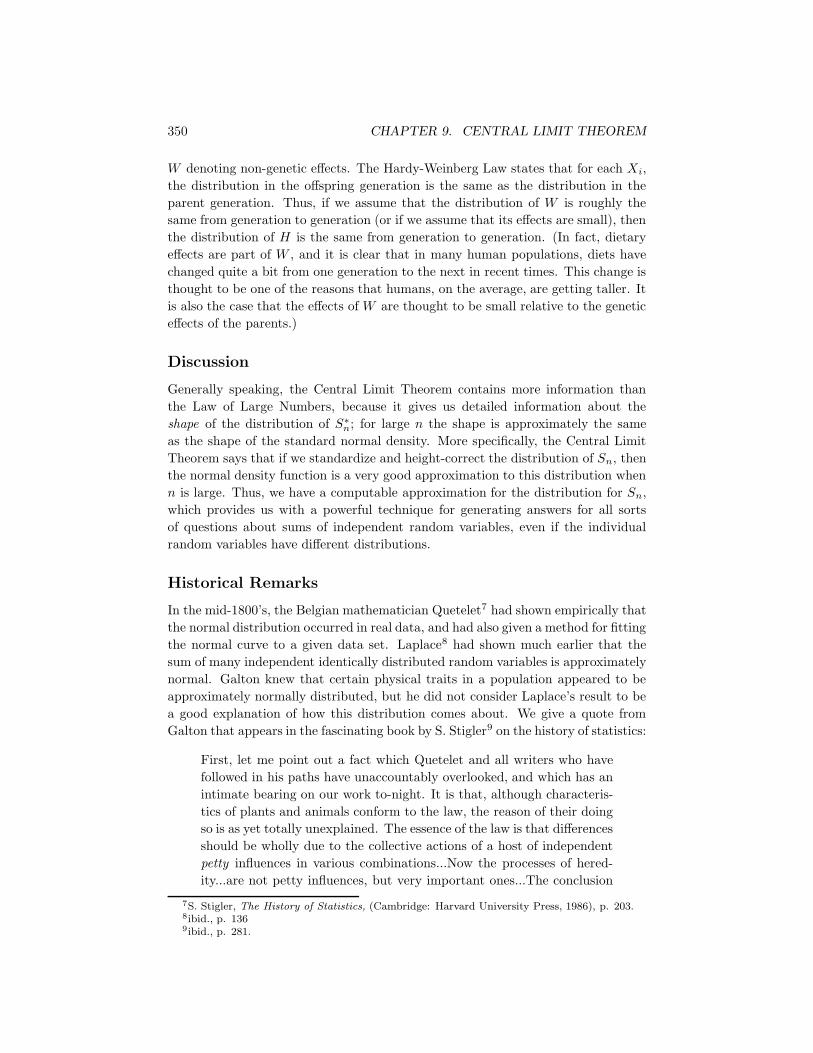
Figure 9.11: Two-stage version of the quincunx.
is...that the processes of heredity must work harmoniously with the law
of deviation, and be themselves in some sense conformable to it.
Galton invented a device known as a quincunx (now commonly called a Galton
board), which we used in Example 3.10 to show how to physically obtain a binomial
distribution. Of course, the Central Limit Theorem says that for large values of
the parameter n, the binomial distribution is approximately normal. Galton used
the quincunx to explain how inheritance affects the distribution of a trait among
offspring.
We consider, as Galton did, what happens if we interrupt, at some intermediate
height, the progress of the shot that is falling in the quincunx. The reader is referred
to Figure 9.11. This figure is a drawing of Karl Pearson,10 based upon Galton’s
notes. In this figure, the shot is being temporarily segregated into compartments at
the line AB. (The line A′B′ forms a platform on which the shot can rest.) If the line
AB is not too close to the top of the quincunx, then the shot will be approximately
normally distributed at this line. Now suppose that one compartment is opened, as
shown in the figure. The shot from that compartment will fall, forming a normal
distribution at the bottom of the quincunx. If now all of the compartments are
10Karl Pearson, The Life, Letters and Labours of Francis Galton, vol. IIIB, (Cambridge at theUniversity Press 1930.) p. 466. Reprinted with permission.
352 CHAPTER 9. CENTRAL LIMIT THEOREM
opened, all of the shot will fall, producing the same distribution as would occur if
the shot were not temporarily stopped at the line AB. But the action of stopping
the shot at the line AB, and then releasing the compartments one at a time, is
just the same as convoluting two normal distributions. The normal distributions at
the bottom, corresponding to each compartment at the line AB, are being mixed,
with their weights being the number of shot in each compartment. On the other
hand, it is already known that if the shot are unimpeded, the final distribution is
approximately normal. Thus, this device shows that the convolution of two normal
distributions is again normal.
Galton also considered the quincunx from another perspective. He segregated
into seven groups, by weight, a set of 490 sweet pea seeds. He gave 10 seeds from
each of the seven group to each of seven friends, who grew the plants from the
seeds. Galton found that each group produced seeds whose weights were normally
distributed. (The sweet pea reproduces by self-pollination, so he did not need to
consider the possibility of interaction between different groups.) In addition, he
found that the variances of the weights of the offspring were the same for each
group. This segregation into groups corresponds to the compartments at the line
AB in the quincunx. Thus, the sweet peas were acting as though they were being
governed by a convolution of normal distributions.
He now was faced with a problem. We have shown in Chapter 7, and Galton
knew, that the convolution of two normal distributions produces a normal distribu-
tion with a larger variance than either of the original distributions. But his data on
the sweet pea seeds showed that the variance of the offspring population was the
same as the variance of the parent population. His answer to this problem was to
postulate a mechanism that he called reversion, and is now called regression to the
mean. As Stigler puts it:11
The seven groups of progeny were normally distributed, but not about
their parents’ weight. Rather they were in every case distributed about
a value that was closer to the average population weight than was that of
the parent. Furthermore, this reversion followed “the simplest possible
law,” that is, it was linear. The average deviation of the progeny from
the population average was in the same direction as that of the parent,
but only a third as great. The mean progeny reverted to type, and
the increased variation was just sufficient to maintain the population
variability.
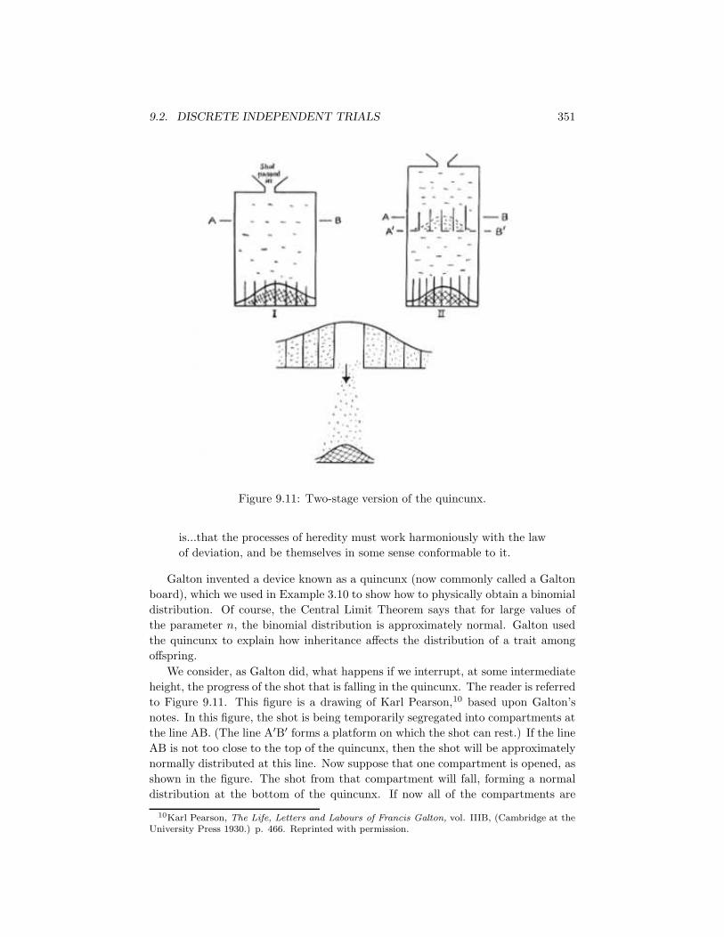
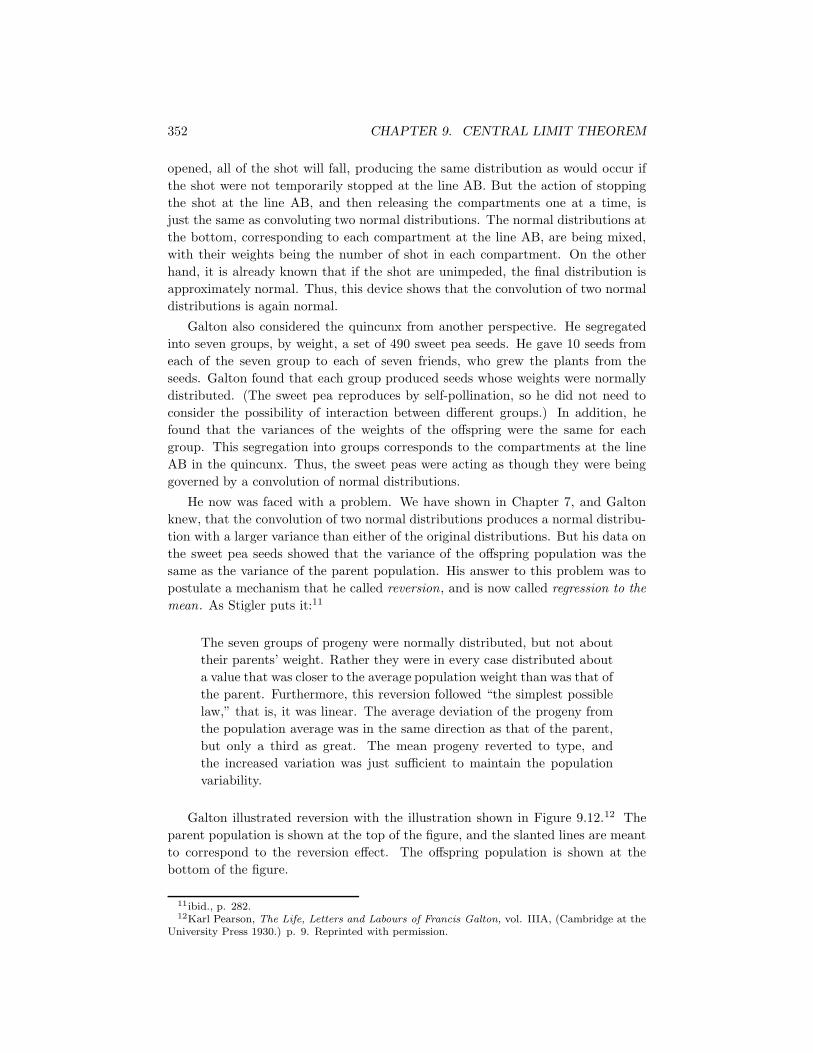
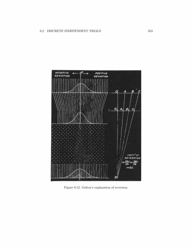
Galton illustrated reversion with the illustration shown in Figure 9.12.12 The
parent population is shown at the top of the figure, and the slanted lines are meant
to correspond to the reversion effect. The offspring population is shown at the
bottom of the figure.
11ibid., p. 282.12Karl Pearson, The Life, Letters and Labours of Francis Galton, vol. IIIA, (Cambridge at the
University Press 1930.) p. 9. Reprinted with permission.
9.2. DISCRETE INDEPENDENT TRIALS 353
Figure 9.12: Galton’s explanation of reversion.
354 CHAPTER 9. CENTRAL LIMIT THEOREM
Exercises
1 A die is rolled 24 times. Use the Central Limit Theorem to estimate the
probability that
(a) the sum is greater than 84.
(b) the sum is equal to 84.
2 A random walker starts at 0 on the x-axis and at each time unit moves 1
step to the right or 1 step to the left with probability 1/2. Estimate the
probability that, after 100 steps, the walker is more than 10 steps from the
starting position.
3 A piece of rope is made up of 100 strands. Assume that the breaking strength
of the rope is the sum of the breaking strengths of the individual strands.
Assume further that this sum may be considered to be the sum of an inde-
pendent trials process with 100 experiments each having expected value of 10
pounds and standard deviation 1. Find the approximate probability that the
rope will support a weight
(a) of 1000 pounds.
(b) of 970 pounds.
4 Write a program to find the average of 1000 random digits 0, 1, 2, 3, 4, 5, 6, 7,
8, or 9. Have the program test to see if the average lies within three standard
deviations of the expected value of 4.5. Modify the program so that it repeats
this simulation 1000 times and keeps track of the number of times the test is
passed. Does your outcome agree with the Central Limit Theorem?
5 A die is thrown until the first time the total sum of the face values of the die
is 700 or greater. Estimate the probability that, for this to happen,
(a) more than 210 tosses are required.
(b) less than 190 tosses are required.
(c) between 180 and 210 tosses, inclusive, are required.
6 A bank accepts rolls of pennies and gives 50 cents credit to a customer without
counting the contents. Assume that a roll contains 49 pennies 30 percent of
the time, 50 pennies 60 percent of the time, and 51 pennies 10 percent of the
time.
(a) Find the expected value and the variance for the amount that the bank
loses on a typical roll.
(b) Estimate the probability that the bank will lose more than 25 cents in
100 rolls.
(c) Estimate the probability that the bank will lose exactly 25 cents in 100
rolls.
9.2. DISCRETE INDEPENDENT TRIALS 355
(d) Estimate the probability that the bank will lose any money in 100 rolls.
(e) How many rolls does the bank need to collect to have a 99 percent chance
of a net loss?
7 A surveying instrument makes an error of −2, −1, 0, 1, or 2 feet with equal
probabilities when measuring the height of a 200-foot tower.
(a) Find the expected value and the variance for the height obtained using
this instrument once.
(b) Estimate the probability that in 18 independent measurements of this
tower, the average of the measurements is between 199 and 201, inclusive.
8 For Example 9.6 estimate P (S30 = 0). That is, estimate the probability that
the errors cancel out and the student’s grade point average is correct.
9 Prove the Law of Large Numbers using the Central Limit Theorem.
10 Peter and Paul match pennies 10,000 times. Describe briefly what each of the
following theorems tells you about Peter’s fortune.
(a) The Law of Large Numbers.
(b) The Central Limit Theorem.
11 A tourist in Las Vegas was attracted by a certain gambling game in which
the customer stakes 1 dollar on each play; a win then pays the customer
2 dollars plus the return of her stake, although a loss costs her only her stake.
Las Vegas insiders, and alert students of probability theory, know that the
probability of winning at this game is 1/4. When driven from the tables by
hunger, the tourist had played this game 240 times. Assuming that no near
miracles happened, about how much poorer was the tourist upon leaving the
casino? What is the probability that she lost no money?
12 We have seen that, in playing roulette at Monte Carlo (Example 6.13), betting
1 dollar on red or 1 dollar on 17 amounts to choosing between the distributions
mX =
( −1 −1/2 1
18/37 1/37 18/37
)
or
mX =
( −1 35
36/37 1/37
)
You plan to choose one of these methods and use it to make 100 1-dollar
bets using the method chosen. Using the Central Limit Theorem, estimate
the probability of winning any money for each of the two games. Compare
your estimates with the actual probabilities, which can be shown, from exact
calculations, to equal .437 and .509 to three decimal places.
13 In Example 9.6 find the largest value of p that gives probability .954 that the
first decimal place is correct.
356 CHAPTER 9. CENTRAL LIMIT THEOREM
14 It has been suggested that Example 9.6 is unrealistic, in the sense that the
probabilities of errors are too low. Make up your own (reasonable) estimate
for the distribution m(x), and determine the probability that a student’s grade
point average is accurate to within .05. Also determine the probability that
it is accurate to within .5.
15 Find a sequence of uniformly bounded discrete independent random variables
{Xn} such that the variance of their sum does not tend to ∞ as n → ∞, and
such that their sum is not asymptotically normally distributed.
9.3 Central Limit Theorem for Continuous Inde-
pendent Trials
We have seen in Section 9.2 that the distribution function for the sum of a large
number n of independent discrete random variables with mean µ and variance σ2
tends to look like a normal density with mean nµ and variance nσ2. What is
remarkable about this result is that it holds for any distribution with finite mean
and variance. We shall see in this section that the same result also holds true for
continuous random variables having a common density function.
Let us begin by looking at some examples to see whether such a result is even
plausible.
Standardized Sums
Example 9.7 Suppose we choose n random numbers from the interval [0, 1] with
uniform density. Let X1, X2, . . . , Xn denote these choices, and Sn = X1 + X2 +
· · · + Xn their sum.
We saw in Example 7.9 that the density function for Sn tends to have a normal
shape, but is centered at n/2 and is flattened out. In order to compare the shapes
of these density functions for different values of n, we proceed as in the previous
section: we standardize Sn by defining
S∗n =
Sn − nµ√nσ
.
Then we see that for all n we have
E(S∗n) = 0 ,
V (S∗n) = 1 .
The density function for S∗n is just a standardized version of the density function
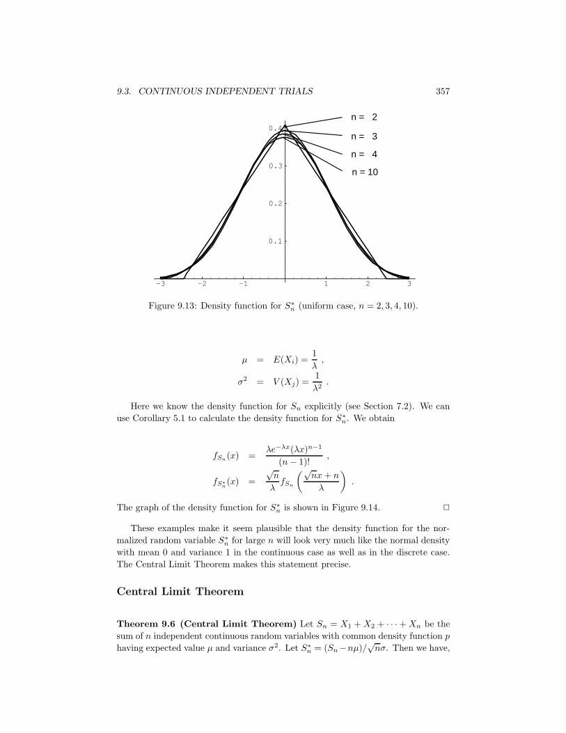
for Sn (see Figure 9.13). 2
Example 9.8 Let us do the same thing, but now choose numbers from the interval
[0, +∞) with an exponential density with parameter λ. Then (see Example 6.26)
9.3. CONTINUOUS INDEPENDENT TRIALS 357
-3 -2 -1 1 2 3
0.1
0.2
0.3
0.4
n = 2
n = 3
n = 4
n = 10
Figure 9.13: Density function for S∗n (uniform case, n = 2, 3, 4, 10).
µ = E(Xi) =1
λ,
σ2 = V (Xj) =1
λ2.
Here we know the density function for Sn explicitly (see Section 7.2). We can
use Corollary 5.1 to calculate the density function for S∗n. We obtain
fSn(x) =
λe−λx(λx)n−1
(n − 1)!,
fS∗
n(x) =
√n
λfSn
(√nx + n
λ
)
.
The graph of the density function for S∗n is shown in Figure 9.14. 2
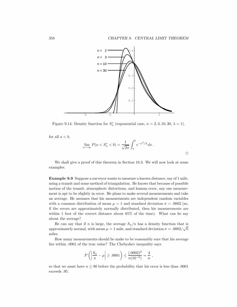
These examples make it seem plausible that the density function for the nor-
malized random variable S∗n for large n will look very much like the normal density
with mean 0 and variance 1 in the continuous case as well as in the discrete case.
The Central Limit Theorem makes this statement precise.
Central Limit Theorem
Theorem 9.6 (Central Limit Theorem) Let Sn = X1 + X2 + · · · + Xn be the
sum of n independent continuous random variables with common density function p
having expected value µ and variance σ2. Let S∗n = (Sn−nµ)/
√nσ. Then we have,
358 CHAPTER 9. CENTRAL LIMIT THEOREM
-4 -2 2
0.1
0.2
0.3
0.4
0.5n = 2
n = 3
n = 10
n = 30
Figure 9.14: Density function for S∗n (exponential case, n = 2, 3, 10, 30, λ = 1).
for all a < b,
limn→∞
P (a < S∗n < b) =
1√2π
∫ b
a
e−x2/2 dx .
2
We shall give a proof of this theorem in Section 10.3. We will now look at some
examples.
Example 9.9 Suppose a surveyor wants to measure a known distance, say of 1 mile,
using a transit and some method of triangulation. He knows that because of possible
motion of the transit, atmospheric distortions, and human error, any one measure-
ment is apt to be slightly in error. He plans to make several measurements and take
an average. He assumes that his measurements are independent random variables
with a common distribution of mean µ = 1 and standard deviation σ = .0002 (so,
if the errors are approximately normally distributed, then his measurements are
within 1 foot of the correct distance about 65% of the time). What can he say
about the average?
He can say that if n is large, the average Sn/n has a density function that is
approximately normal, with mean µ = 1 mile, and standard deviation σ = .0002/√
n
miles.
How many measurements should he make to be reasonably sure that his average
lies within .0001 of the true value? The Chebyshev inequality says
P
(∣
∣
∣
∣
Sn
n− µ
∣
∣
∣
∣
≥ .0001
)
≤ (.0002)2
n(10−8)=
4
n,
so that we must have n ≥ 80 before the probability that his error is less than .0001
exceeds .95.
9.3. CONTINUOUS INDEPENDENT TRIALS 359
We have already noticed that the estimate in the Chebyshev inequality is not
always a good one, and here is a case in point. If we assume that n is large enough
so that the density for Sn is approximately normal, then we have
P
(∣
∣
∣
∣
Sn
n− µ
∣
∣
∣
∣
< .0001
)
= P(
−.5√
n < S∗n < +.5
√n)
≈ 1√2π
∫ +.5√
n
−.5√
n
e−x2/2 dx ,
and this last expression is greater than .95 if .5√
n ≥ 2. This says that it suffices
to take n = 16 measurements for the same results. This second calculation is
stronger, but depends on the assumption that n = 16 is large enough to establish
the normal density as a good approximation to S∗n, and hence to Sn. The Central
Limit Theorem here says nothing about how large n has to be. In most cases
involving sums of independent random variables, a good rule of thumb is that for
n ≥ 30, the approximation is a good one. In the present case, if we assume that the
errors are approximately normally distributed, then the approximation is probably
fairly good even for n = 16. 2
Estimating the Mean
Example 9.10 (Continuation of Example 9.9) Now suppose our surveyor is mea-
suring an unknown distance with the same instruments under the same conditions.
He takes 36 measurements and averages them. How sure can he be that his mea-
surement lies within .0002 of the true value?
Again using the normal approximation, we get
P
(∣
∣
∣
∣
Sn
n− µ
∣
∣
∣
∣
< .0002
)
= P(
|S∗n| < .5
√n)
≈ 2√2π
∫ 3
−3
e−x2/2 dx
≈ .997 .
This means that the surveyor can be 99.7 percent sure that his average is within
.0002 of the true value. To improve his confidence, he can take more measurements,
or require less accuracy, or improve the quality of his measurements (i.e., reduce
the variance σ2). In each case, the Central Limit Theorem gives quantitative infor-
mation about the confidence of a measurement process, assuming always that the
normal approximation is valid.
Now suppose the surveyor does not know the mean or standard deviation of his
measurements, but assumes that they are independent. How should he proceed?
Again, he makes several measurements of a known distance and averages them.
As before, the average error is approximately normally distributed, but now with
unknown mean and variance. 2
360 CHAPTER 9. CENTRAL LIMIT THEOREM
Sample Mean
If he knows the variance σ2 of the error distribution is .0002, then he can estimate
the mean µ by taking the average, or sample mean of, say, 36 measurements:
µ̄ =x1 + x2 + · · · + xn
n,
where n = 36. Then, as before, E(µ̄) = µ. Moreover, the preceding argument shows
that
P (|µ̄ − µ| < .0002) ≈ .997 .
The interval (µ̄− .0002, µ̄+ .0002) is called the 99.7% confidence interval for µ (see
Example 9.4).
Sample Variance
If he does not know the variance σ2 of the error distribution, then he can estimate
σ2 by the sample variance:
σ̄2 =(x1 − µ̄)2 + (x2 − µ̄)2 + · · · + (xn − µ̄)2
n,
where n = 36. The Law of Large Numbers, applied to the random variables (Xi −µ̄)2, says that for large n, the sample variance σ̄2 lies close to the variance σ2, so
that the surveyor can use σ̄2 in place of σ2 in the argument above.
Experience has shown that, in most practical problems of this type, the sample
variance is a good estimate for the variance, and can be used in place of the variance
to determine confidence levels for the sample mean. This means that we can rely
on the Law of Large Numbers for estimating the variance, and the Central Limit
Theorem for estimating the mean.
We can check this in some special cases. Suppose we know that the error distri-
bution is normal, with unknown mean and variance. Then we can take a sample of
n measurements, find the sample mean µ̄ and sample variance σ̄2, and form
T ∗n =
Sn − nµ̄√nσ̄
,
where n = 36. We expect T ∗n to be a good approximation for S∗
n for large n.
t-Density
The statistician W. S. Gosset13 has shown that in this case T ∗n has a density function
that is not normal but rather a t-density with n degrees of freedom. (The number
n of degrees of freedom is simply a parameter which tells us which t-density to use.)
In this case we can use the t-density in place of the normal density to determine
confidence levels for µ. As n increases, the t-density approaches the normal density.
Indeed, even for n = 8 the t-density and normal density are practically the same
(see Figure 9.15).
13W. S. Gosset discovered the distribution we now call the t-distribution while working for theGuinness Brewery in Dublin. He wrote under the pseudonym “Student.” The results discussed herefirst appeared in Student, “The Probable Error of a Mean,” Biometrika, vol. 6 (1908), pp. 1-24.
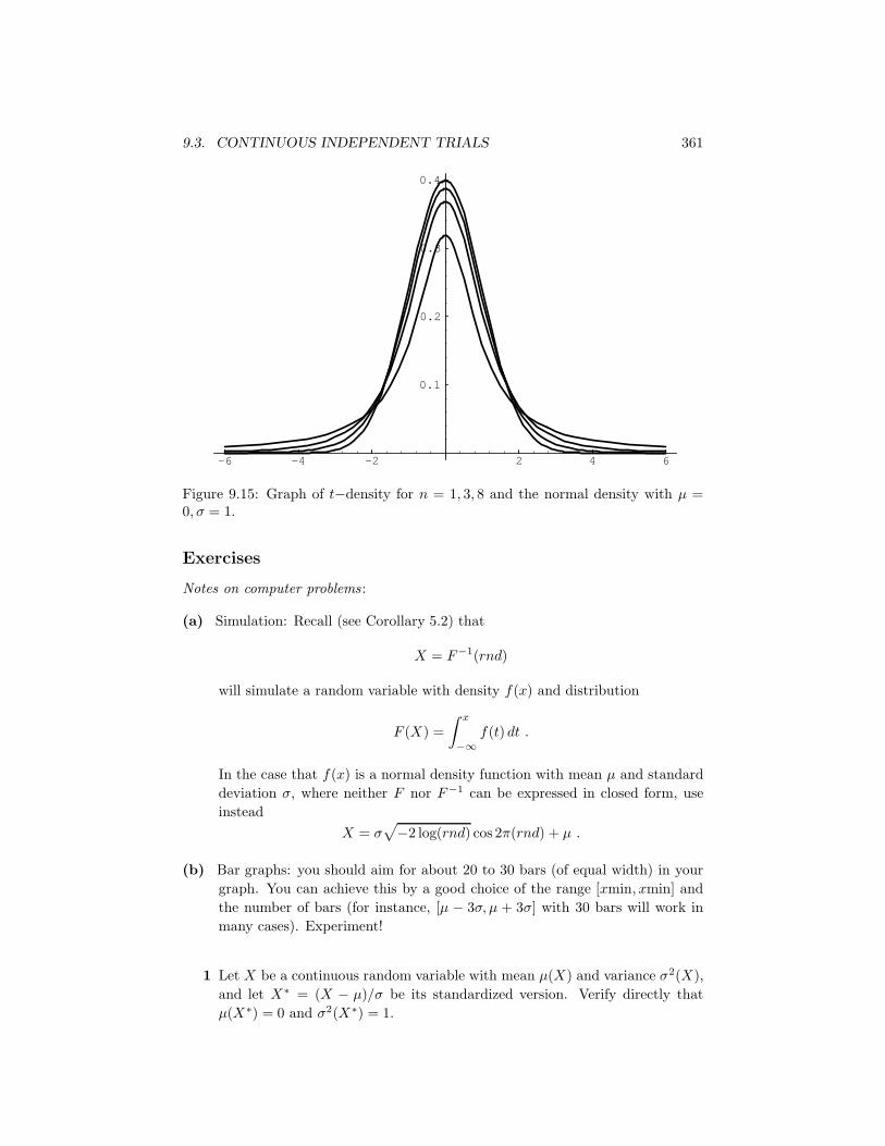
9.3. CONTINUOUS INDEPENDENT TRIALS 361
-6 -4 -2 2 4 6
0.1
0.2
0.3
0.4
Figure 9.15: Graph of t−density for n = 1, 3, 8 and the normal density with µ =0, σ = 1.
Exercises
Notes on computer problems :
(a) Simulation: Recall (see Corollary 5.2) that
X = F−1(rnd)
will simulate a random variable with density f(x) and distribution
F (X) =
∫ x
−∞f(t) dt .
In the case that f(x) is a normal density function with mean µ and standard
deviation σ, where neither F nor F−1 can be expressed in closed form, use
instead
X = σ√
−2 log(rnd) cos 2π(rnd) + µ .
(b) Bar graphs: you should aim for about 20 to 30 bars (of equal width) in your
graph. You can achieve this by a good choice of the range [xmin, xmin] and
the number of bars (for instance, [µ − 3σ, µ + 3σ] with 30 bars will work in
many cases). Experiment!
1 Let X be a continuous random variable with mean µ(X) and variance σ2(X),
and let X∗ = (X − µ)/σ be its standardized version. Verify directly that
µ(X∗) = 0 and σ2(X∗) = 1.
362 CHAPTER 9. CENTRAL LIMIT THEOREM
2 Let {Xk}, 1 ≤ k ≤ n, be a sequence of independent random variables, all with
mean 0 and variance 1, and let Sn, S∗n, and An be their sum, standardized
sum, and average, respectively. Verify directly that S∗n = Sn/
√n =
√nAn.
3 Let {Xk}, 1 ≤ k ≤ n, be a sequence of random variables, all with mean µ and
variance σ2, and Yk = X∗k be their standardized versions. Let Sn and Tn be
the sum of the Xk and Yk, and S∗n and T ∗
n their standardized version. Show
that S∗n = T ∗
n = Tn/√
n.
4 Suppose we choose independently 25 numbers at random (uniform density)
from the interval [0, 20]. Write the normal densities that approximate the
densities of their sum S25, their standardized sum S∗25, and their average A25.
5 Write a program to choose independently 25 numbers at random from [0, 20],
compute their sum S25, and repeat this experiment 1000 times. Make a bar
graph for the density of S25 and compare it with the normal approximation
of Exercise 4. How good is the fit? Now do the same for the standardized
sum S∗25 and the average A25.
6 In general, the Central Limit Theorem gives a better estimate than Cheby-
shev’s inequality for the average of a sum. To see this, let A25 be the
average calculated in Exercise 5, and let N be the normal approximation
for A25. Modify your program in Exercise 5 to provide a table of the function
F (x) = P (|A25 − 10| ≥ x) = fraction of the total of 1000 trials for which
|A25 − 10| ≥ x. Do the same for the function f(x) = P (|N − 10| ≥ x). (You
can use the normal table, Table 9.4, or the procedure NormalArea for this.)
Now plot on the same axes the graphs of F (x), f(x), and the Chebyshev
function g(x) = 4/(3x2). How do f(x) and g(x) compare as estimates for
F (x)?
7 The Central Limit Theorem says the sums of independent random variables
tend to look normal, no matter what crazy distribution the individual variables
have. Let us test this by a computer simulation. Choose independently 25
numbers from the interval [0, 1] with the probability density f(x) given below,
and compute their sum S25. Repeat this experiment 1000 times, and make up
a bar graph of the results. Now plot on the same graph the density φ(x) =
normal (x, µ(S25), σ(S25)). How well does the normal density fit your bar
graph in each case?
(a) f(x) = 1.
(b) f(x) = 2x.
(c) f(x) = 3x2.
(d) f(x) = 4|x − 1/2|.(e) f(x) = 2− 4|x − 1/2|.
8 Repeat the experiment described in Exercise 7 but now choose the 25 numbers
from [0,∞), using f(x) = e−x.
9.3. CONTINUOUS INDEPENDENT TRIALS 363
9 How large must n be before Sn = X1+X2+· · ·+Xn is approximately normal?
This number is often surprisingly small. Let us explore this question with a
computer simulation. Choose n numbers from [0, 1] with probability density
f(x), where n = 3, 6, 12, 20, and f(x) is each of the densities in Exercise 7.
Compute their sum Sn, repeat this experiment 1000 times, and make up a
bar graph of 20 bars of the results. How large must n be before you get a
good fit?
10 A surveyor is measuring the height of a cliff known to be about 1000 feet.
He assumes his instrument is properly calibrated and that his measurement
errors are independent, with mean µ = 0 and variance σ2 = 10. He plans to
take n measurements and form the average. Estimate, using (a) Chebyshev’s
inequality and (b) the normal approximation, how large n should be if he
wants to be 95 percent sure that his average falls within 1 foot of the true
value. Now estimate, using (a) and (b), what value should σ2 have if he wants
to make only 10 measurements with the same confidence?
11 The price of one share of stock in the Pilsdorff Beer Company (see Exer-
cise 8.2.12) is given by Yn on the nth day of the year. Finn observes that
the differences Xn = Yn+1 − Yn appear to be independent random variables
with a common distribution having mean µ = 0 and variance σ2 = 1/4. If
Y1 = 100, estimate the probability that Y365 is
(a) ≥ 100.
(b) ≥ 110.
(c) ≥ 120.
12 Test your conclusions in Exercise 11 by computer simulation. First choose
364 numbers Xi with density f(x) = normal(x, 0, 1/4). Now form the sum
Y365 = 100 + X1 + X2 + · · · + X364, and repeat this experiment 200 times.
Make up a bar graph on [50, 150] of the results, superimposing the graph of the
approximating normal density. What does this graph say about your answers
in Exercise 11?
13 Physicists say that particles in a long tube are constantly moving back and
forth along the tube, each with a velocity Vk (in cm/sec) at any given moment
that is normally distributed, with mean µ = 0 and variance σ2 = 1. Suppose
there are 1020 particles in the tube.
(a) Find the mean and variance of the average velocity of the particles.
(b) What is the probability that the average velocity is ≥ 10−9 cm/sec?
14 An astronomer makes n measurements of the distance between Jupiter and
a particular one of its moons. Experience with the instruments used leads
her to believe that for the proper units the measurements will be normally
364 CHAPTER 9. CENTRAL LIMIT THEOREM
distributed with mean d, the true distance, and variance 16. She performs a
series of n measurements. Let
An =X1 + X2 + · · · + Xn
n
be the average of these measurements.
(a) Show that
P
(
An − 8√n≤ d ≤ An +
8√n
)
≈ .95.
(b) When nine measurements were taken, the average of the distances turned
out to be 23.2 units. Putting the observed values in (a) gives the 95 per-
cent confidence interval for the unknown distance d. Compute this in-
terval.
(c) Why not say in (b) more simply that the probability is .95 that the value
of d lies in the computed confidence interval?
(d) What changes would you make in the above procedure if you wanted to
compute a 99 percent confidence interval?
15 Plot a bar graph similar to that in Figure 9.10 for the heights of the mid-
parents in Galton’s data as given in Appendix B and compare this bar graph
to the appropriate normal curve.