Embed Size (px)
Citation preview
Federal Reserve Bank of New York
Staff Reports
Central Bank Transparency, the Accuracy of Professional
Forecasts, and Interest Rate Volatility
Menno Middeldorp
Staff Report no. 496
May 2011
This paper presents preliminary findings and is being distributed to economists
and other interested readers solely to stimulate discussion and elicit comments.
The views expressed in this paper are those of the author and are not necessarily
reflective of views at the Federal Reserve Bank of New York or the Federal
Reserve System. Any errors or omissions are the responsibility of the author.
Central Bank Transparency, the Accuracy of Professional Forecasts,
and Interest Rate Volatility
Menno Middeldorp
Federal Reserve Bank of New York Staff Reports, no. 496
May 2011
JEL classification: D83, E47, E58, G14
Abstract
Central banks worldwide have become more transparent. An important reason is that
democratic societies expect more openness from public institutions. Policymakers also see
transparency as a way to improve the predictability of monetary policy, thereby lowering
interest rate volatility and contributing to economic stability. Most empirical studies
support this view. However, there are three reasons why more research is needed. First,
some (mostly theoretical) work suggests that transparency has an adverse effect on
predictability. Second, empirical studies have mostly focused on average predictability
before and after specific reforms in a small set of advanced economies. Third, less is
known about the effect on interest rate volatility. To extend the literature, I use the Dincer
and Eichengreen (2007) transparency index for twenty-four economies of varying income
and examine the impact of transparency on both predictability and market volatility. I find
that higher transparency improves the accuracy of interest rate forecasts for three months
ahead and reduces rate volatility.
Key words: Central bank communication, interest rate forecasts, central bank
transparency, financial market efficiency
Middeldorp: Federal Reserve Bank of New York and Utrecht University
([email protected]). The author gratefully acknowledges the support of the Institute for
Monetary Research of the Hong Kong Monetary Authority (HKMA), where most of the research
was conducted in the context of a doctoral dissertation for Utrecht University. Thanks also to
Qianying Chen, Deborah Perelmuter, Matthew Raskin, Stephanie Rosenkranz, and participants at an
HKMA seminar for useful questions and comments. Special thanks to Clemens Kool for extensive
comments on several drafts. The views expressed in the paper are those of the author and do not
necessarily reflect the position of the Federal Reserve Bank of New York or the Federal Reserve
System. Any errors or omissions are the responsibility of the author.
1 Overview
Central banks worldwide have become considerably more transparent aboutmonetary policy, including defining their goals, explaining decisions, releasingeconomic forecasts and providing guidance about future policy. Between 1998and 2005, 89 of the 100 countries in the Dincer and Eichengreen (2007) indexshow an increase in transparency and none a decline. An important reason isthat (the increased number of) democratic societies expect more openness frompublic institutions. Another motivation for greater transparency is a reductionin monetary policy surprises to thereby reduce accompanying financial marketand economic volatility. Along these lines, Bernanke (2004) asserts that, “clearcommunication helps to increase the near-term predictability of [central bank]1
rate decisions, which reduces risk and volatility in financial markets and allowsfor smoother adjustment of the economy to rate changes.”This paper focuseson the benefits Bernanke describes, by examining transparency’s impact bothon predictability and interest rate volatility.
As discussed in the literature review in Section 2, Although straightforwardintuition and standard financial market theory suggest that transparency shouldenhance predictability, this has been challenged by some theoretical and exper-imental research, that shows that under some circumstances transparency canreduce the use of private information and thereby actually damage predictabil-ity.
Nevertheless, a considerable body of empirical research suggests that trans-parency improves predictability. The focus in empirical work has largely beenon fixed income markets, for at least three reasons. First, they provide a readilyavailable measure of monetary policy expectations. Second, they provide themost immediate avenue through which the central bank’s own interest ratesaffect the economy. Third, central banks are often concerned with the volatil-ity of interest rates and thus averse to surprising markets, as the quote aboveillustrates.
Three approaches have been used to assess the impact of greater trans-parency on predictability. First, testing the extent to which market pricesreact to central bank decisions, second, examining forecast errors of expecta-tions priced into the yield curve or futures and third, studying the accuracy ofpredictions by professional forecasters.
Each approach has its own advantages and disadvantages. In this paperI use private sector forecasts of money market interest rates for four reasons.First, these represent a straightforward measure of expectations. Second, theyare available for a broad set of countries. Third, they are available for fore-
1Originally “FOMC” for the Federal Open Market Committee, the body that sets USmonetary policy; clearly the same reasoning applies to any other central bank.
1
cast horizons out to a year. Fourth and importantly, it is possible to observeindividual forecasts.
Despite the significant number of papers, there is still room for improve-ment in the empirical literature. Most studies only examine a limited numberof advanced countries. They do this largely by comparing average predictabilitybefore and after specific reforms in communication policy. As a result, there isno real understanding of the relationship between varying levels of transparency(across time and space) and corresponding variations in predictability. The re-search presented in this paper addresses these gaps in the literature by utilizingthe Dincer and Eichengreen (2007) index along with professional interest rateforecasts to study varying levels of transparency across 24 countries with differ-ing levels of economic development. Because one goal of improving monetarypolicy predictability is to reduce financial market and economic volatility, thispaper also examines the impact of transparency on interest rate volatility.
To establish a relationship between transparency, predictability and interestrate volatility requires measures of all three. In Section 3, I give a detaileddescription of datasets that can be used to do this. To measure transparency Iemploy the Dincer and Eichengreen (2007) index, which essentially counts thenumber of transparency enhancing institutions of each central bank. To measurepredictability I use the error of professional interest rate forecasts at both threeand twelve month horizons. To measure interest rate volatility I use the historicstandard deviation of the same interest rates.
Section 4 describes formally how public information could impact forecasts ofinterest rates and interest rate volatility. If an increase in transparency only im-proves public information then it will result in individual forecasts that becomemore accurate. However, if transparency has a negative impact on private infor-mation, as the theoretical and experimental research discussed below suggests,it could also lead to higher errors. Theoretically, market volatility behaves sim-ilarly to predictability, more public information should dampen volatility unlessit hampers private information.
As shown in Section 5, simple graphs and panel regression results suggestthat transparency enhances predictability. Forecast errors decline significantlyat the three month horizon, but not at twelve months ahead. Transparency alsolowers volatility. Overall the evidence suggests that transparency can indeedserve the goal outlined by Bernanke (2004), i.e. improving predictability helpsto foster lower interest rate volatility.
2
2 Review of the literature on predictability
The literature on central bank transparency and communication has grownrapidly over the last decade and now consists of hundreds of papers and arti-cles. Different angles have been pursued. Many papers examine the implicationsof transparency in theoretical macroeconomic models. Others examine empiri-cally if transparency has influenced inflation and other macroeconomic variables.The impact of transparency on the financial markets has also been an impor-tant theme in the literature. Especially around the turn of the century, manyarticles examined if central bank communication had some impact on the finan-cial markets, generally concluding that it does. The question addressed heregoes a step further, asking whether transparency improves the predictability ofmonetary policy in the financial markets. This section reviews the theoretical,experimental and empirical evidence to date and highlights gaps in the liter-ature that are addressed by research described in the remainder of the paper.Blinder, Ehrmann, Fratzscher, de Haan and Jansen (2008) and van der Cruijsenand Eijffi nger (2007) offer broader overviews of the literature on transparency.
2.1 Theory
Intuitively, one would expect better public information to improve market func-tioning, in the sense that financial markets become better at predicting theoutcome of unrealized fundamentals. This is true in a basic rational expec-tations asset market model with exogenous public and private information.2
Under different assumptions or models, however, better public information canhamper market functioning.
Probably the best known example is Morris and Shin (2002). They presenta model where the profits of individual agents depend not only on fundamentalvalues but also on the expectations of others (clearly an issue in any marketwhere assets can be sold before the realization of their fundamental value).Under these circumstances a suffi ciently clear signal from the central bank canact as a coordinating point that could distract market participants from theirprivate information and possibly fundamentals. Svensson (2006) argues that thisconclusion is only valid for the unlikely situation where public signals are lessprecise than private information. However, Demertzis and Hoeberichts (2007)add costly information acquisition to Morris and Shin (2002)’s model and findthat it strengthens their result.
Another theoretical model by Dale, Orphanides and Osterholm (2008) demon-strates that if the private sector is not able to learn the precision of the centralbank’s information, it may overreact to central bank communication. Kool et al.
2See Kool, Middeldorp and Rosenkranz (2011), where the case of exogenous private infor-mation is equivalent to holding the fraction of informed traders constant.
3
(2011) find that public information can crowd out investment in private informa-tion, which hampers predictability, a conclusion supported by the experimentalwork of Middeldorp and Rosenkranz (2011).
2.2 Empirical studies
Many empirical research papers have tried to assess if transparency improvesthe predictability of monetary policy in the financial markets.3 The generalapproach is to select a watershed communication reform and test the differencebetween predictability before and afterwards. US studies typically use the firstannouncement of the Federal Open Market Committee’s (FOMC) rate decisionsin February 1994, while for other countries the introduction of an inflationtarget, with its accompanying communication tools, is used. One can measurepredictability in at least three ways. The first is to ascertain how surprisedmarkets are by policy decisions. The second extracts expectations from theyield curve or futures to see how accurate they are. The third uses professionalforecasts of interest rates. Taken together the evidence to date suggests thattransparency improves predictability.
The first approach to assessing the predictability of monetary policy involvesexamining market movements close to policy decisions. Little reaction in moneymarket rates following a policy rate change suggests that it has been priced inand that policy is predictable. Money market movements prior to the decisionin the same direction as the rate change can be interpreted as anticipating themove. Swanson (2006) finds that US interest rates show less reaction to Feddecisions over the period where the Fed reformed its communication policy.Holmsen, Qvigstad, Øistein Røisland and Solberg-Johansen (2008) find lowervolatility on the days the Norges Bank announced its decisions after it startedto release forecasts of its own interest rates. Murdzhev and Tomljanovich (2006)and Coppel and Connolly (2003) show that policy changes are better anticipatedin, respectively, six and eight advanced economies. Although such an approach isfairly intuitive and clear cut, its disadvantage is that it only provides a measureof market expectations between meetings and at the time of rate announcements.Communication reforms that allow market interest rates to anticipate monetarypolicy earlier than one meeting ahead can’t be identified.
A second method is to measure market expectations of monetary policyand examine how accurate these are. Typically expectations are either ex-tracted from the yield curve or futures data. Here too, findings suggest that
3A related strand of the literature does not address predictability in the financial marketsbut examines the usefulness of central bank communication in contructing forecasts of mon-etary policy. Some studies have simply asked if communications contain predictive power initself; examples include Mizen (2009) and Jansen and de Haan (2009). Other studies exam-ine if communication is useful in improving models that forecast monetary policy, such asthe Taylor rule; recent examples are Sturm and de Haan (2009) for the ECB and Hayo andNeuenkirch (2009) for the FOMC.
4
transparency improves predictability. Rafferty and Tomljanovich (2002) andLange, Sack and Whitesell (2003) find better accuracy for the US Treasuryyield curve. Lildholdt and Wetherilt (2004) use a term structure model to showan improvement in the predictability of UK monetary policy. Similarly, Toml-janovich (2004) extracts expectations from bond yield curves and finds thatforecast errors decline in seven advanced economies after transparency reforms.
Regarding futures rates, Swanson (2006) and Carlson, Craig, Higgins andMelick (2006) find that the Fed funds futures are better able to predict USmonetary policy after communication reforms. Kwan (2007) concludes thatforward looking language or guidance, introduced in 2003, has helped to lowerthe average error between the Fed funds futures and the actual outcome of theFed funds rate.
The disadvantage of using bond market expectations, is that such estimatesare likely to be biased. The failure of the expectations hypothesis for the Trea-sury yield curve is a well-documented empirical result (e.g. Cochrane and Pi-azzesi (2005), Campbell and Shiller (1991), Stambaugh (1988), Fama and Bliss(1987)). Risk premiums on interest rates are positive on average and time-varying. Sack (2004) and Piazzesi and Swanson (2008) show that Fed fundsfutures rates also include risk premiums, particularly at longer maturities. Pi-azzesi and Swanson (2008) demonstrate how to adjust Fed funds futures ratesfor time-varying risk premiums using business cycle data. Middeldorp (2011)contributes to the literature on transparency by applying their correction to thequestion of the accuracy of the Fed funds futures.
A third approach is to use predictions by professional forecasters. Theseare a direct measure of expectations, without risk premiums, and also allowone to observe individual forecasts. There are several studies that look at USinterest rates. Swanson (2006) finds an improvement in the accuracy of pri-vate sector interest rate forecasts. Berger, Ehrmann and Fratzscher (2006) findthat communication reduces the disparity of Fed funds target rate predictionsproduced by forecasters from different locations. Hayford and Malliaris (2007)and Bauer, Eisenbeis, Waggoner and Zha (2006) find declining dispersion in UST-bill forecasts. Regarding other central banks, Mariscal and Howells (2006b)find a growing dispersion of private sector forecasts of Bundesbank and ECBmonetary policy up to 2005, a result which runs counter to that for most othersstudies, including that of their own (2006b) research for the Bank of England.
Several multi-country studies use professional forecasts, but they generallyfocus on economic rather than interest rate forecasts. Johnson (2002) shows adecline in inflation forecasts, but not in errors or variance, in an eleven countrypanel. Crowe (2006) finds a convergence of inflation forecasts for eleven infla-tion targeters. Crowe and Meade (2008) demonstrate a convergence of inflationforecasts in line with increasing transparency as measured by an index. Cec-chetti and Hakkio (2009), on the other hand, do not find convincing evidence ofa reduction in the dispersion of inflation forecasts in a sample of 15 countries.
5
Ehrmann, Eijffi nger and Fratzscher (2010) use various measures of central banktransparency to show a convergence of professional forecasts of both economicvariables and interest rates in twelve advanced economies. To my knowledge,there are no studies like the one presented in this paper, that focus on interestrate forecasts using multi-country panel data.
A disadvantage of professional forecasts versus the expectations embedded ininterest rates is that it is not obvious that they are relevant to the transmissionof monetary policy. It is, nevertheless, likely that they both reflect and influencemonetary policy expectations. Large financial institutions are the most commonemployers of professional forecasters and their views are actively dispersed tomarket participants and widely reported on in the press.
Although there is a significant number of empirical studies, they are lim-ited in scope, both in their measure of transparency and geography. The vastmajority of the empirical research discussed above only shows that the averagepredictability was higher after a particular communication reform than it wasbefore. This provides only a binary measure of transparency that gives littlesense of how much transparency has improved. Regarding geographic scope,studies have been conducted for a limited number of advanced economies, typ-ically one country at a time. To address these issues I use a measure of trans-parency with a higher resolution, namely the Dincer and Eichengreen (2007)index, which uses a 15 point scale. Combined with the available data on in-terest rate forecasts, this produces a panel of 24 countries of varying levels ofincome, which provides much greater geographic scope than earlier research.
6
3 Data
To establish the connection of transparency to interest rate predictability andvolatility, one needs adequate measures of all three. I use the Dincer and Eichen-green (2007) index to measure transparency. It grades central banks accordingto the different types of information disclosed. Its main advantage is that itcovers a larger set of countries and periods than earlier measures.
Predictability is measured by the absolute error between private sector moneymarket forecasts reported by Consensus Economics and realized market rates.The advantages and disadvantages of using professional forecasts were discussedin the literature review.
To examine if transparency also impacts the volatility of interest rates, I alsoincorporate the standard deviation of interest rates into the dataset.
Transparency is unlikely to be the only determinant of either predictabilityor volatility. Therefore, to control for overall perceptions of risk I utilize thecommonly used financial risk indices of the PRS Group.
3.1 Transparency index
Different measures of transparency have been assembled and corresponding datacollected by various researchers. The approach was pioneered by Eijffi nger andGeraats (2006), who measure transparency by scoring central banks on a check-list of 15 different types of disclosure, which are grouped into five categories: po-litical, economic, procedural, policy and operational (see the Appendix). Theirmeasure of transparency is based on the simple idea that more types of dis-closure represent greater transparency. A disadvantage is that the quality ofthe information provided is neglected. On the other hand, precisely by avoid-ing additional interpretation it is possible to create an objective measure oftransparency over a wide variety of central banks.
Eijffi nger and Geraats (2006) only have data available for nine advancedeconomies and for just the years 1998 and 2002. Crowe and Meade (2008) as-semble data for 37 countries, following the same approach. Their data, however,is only available for 1998 and 2006, but not in between. Dincer and Eichengreen(2007) also employ the same method but gather data for a hundred countriesfor every year between 1998 and 2005. The scope of their dataset clearly sur-passes other data sources, which is why it is used in this paper. However, dueto the necessary availability of both the transparency data and the surveys ofprofessional forecasts discussed below, only 24 of the hundred countries studiedby Dincer and Eichengreen (2007) can be used.
7
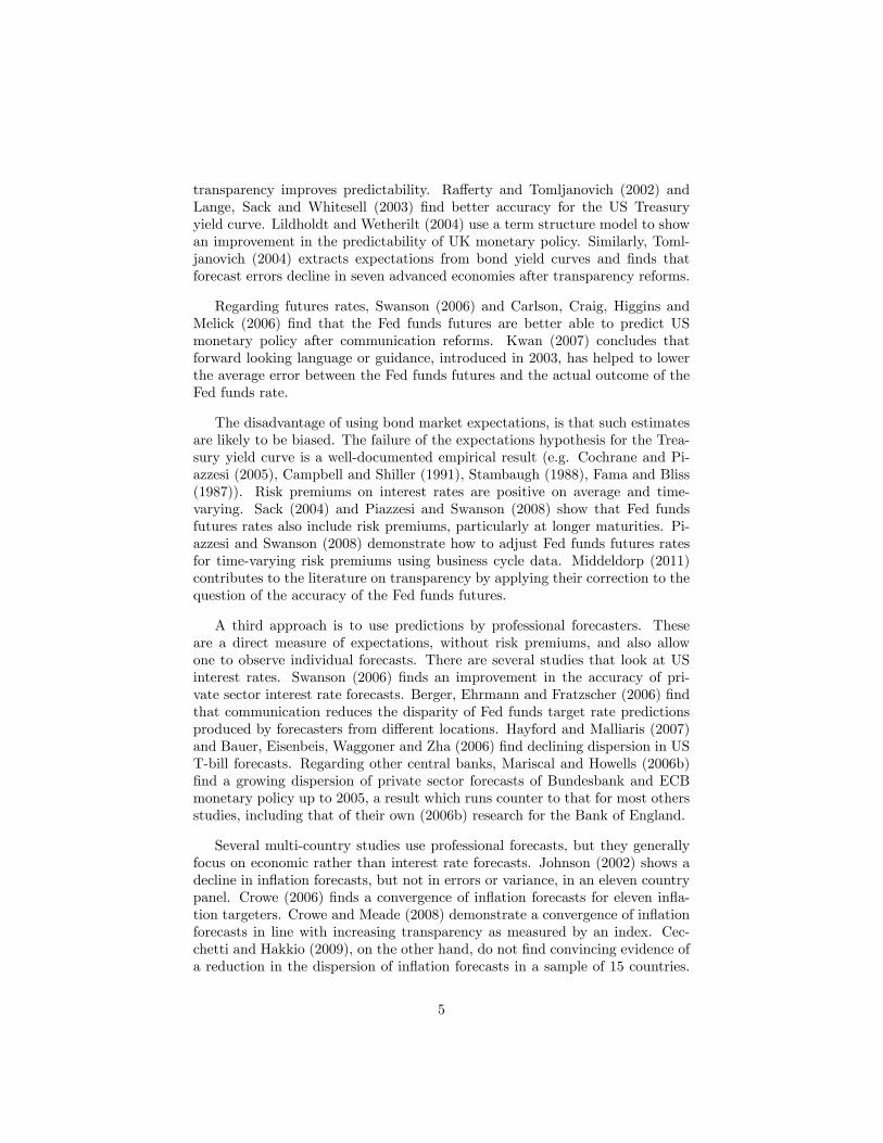
Dincer and Eichengreen (2007) compare the disclosure checklist to the prac-tice of central banks as documented on their websites and in their statutes,annual reports and other published documents. For some items half points areawarded. The approach followed results in a score for each central bank of be-tween 0 and 15 for each year. Where reforms were introduced during the year,the score is based on the disclosures that existed during most of the year.
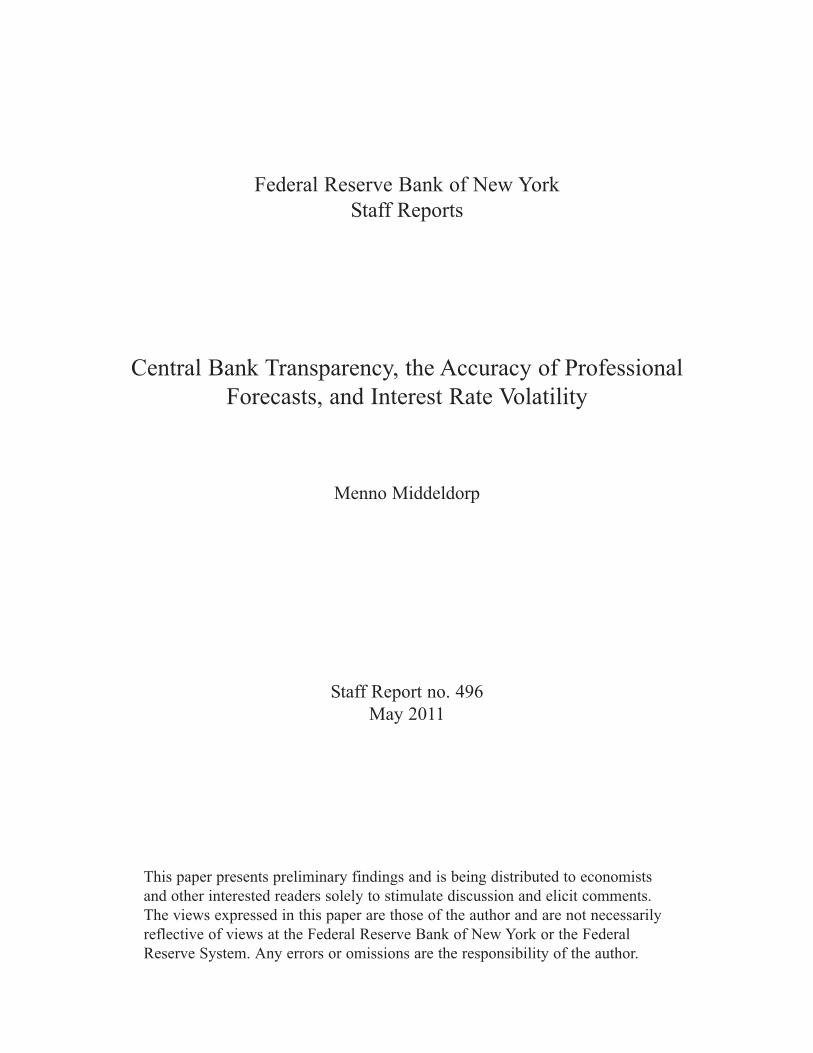
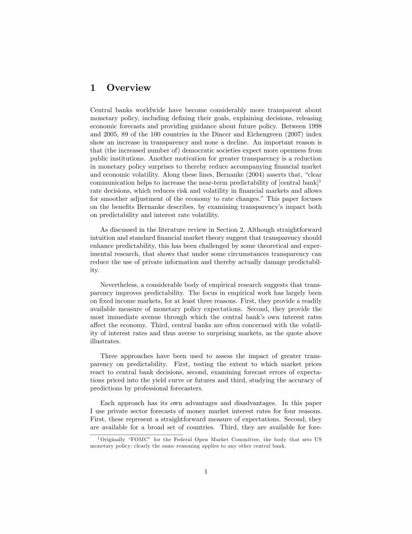
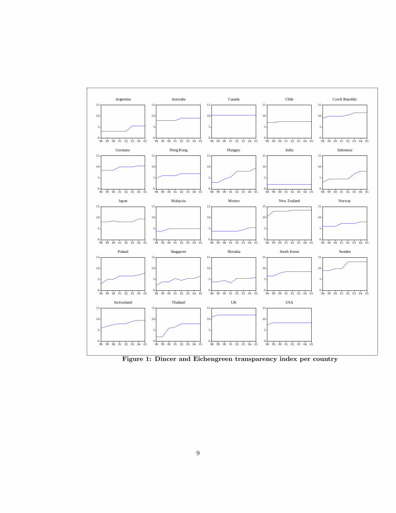
Levels of transparency vary greatly over the sample studied in this paper,both over space and time. India only scores a 2 on the index compared to 13.5for New Zealand in 2005 (see Figure 1 and Table 1). In between there is noconcentration at any particular level of transparency. Lower-income economiestend to have lower levels of transparency, but this is not a hard-and-fast rule; theCzech Republic and Hungary are more transparent than the US while Norway isas transparent as Indonesia. Transparency has increased substantially over themajority of the countries studied and no country saw a decrease in transparency(see Figure 1 and Table 1). Although the three nations that show the largestincrease in transparency are lower-income economies, the rates of improvementdo not seem to be strongly associated with income levels.
8
0
5
10
15
98 99 00 01 02 03 04 05
Argentina
0
5
10
15
98 99 00 01 02 03 04 05
Australia
0
5
10
15
98 99 00 01 02 03 04 05
Canada
0
5
10
15
98 99 00 01 02 03 04 05
Chile
0
5
10
15
98 99 00 01 02 03 04 05
Czech Republic
0
5
10
15
98 99 00 01 02 03 04 05
Germany
0
5
10
15
98 99 00 01 02 03 04 05
Hong Kong
0
5
10
15
98 99 00 01 02 03 04 05
Hungary
0
5
10
15
98 99 00 01 02 03 04 05
India
0
5
10
15
98 99 00 01 02 03 04 05
Indonesia
0
5
10
15
98 99 00 01 02 03 04 05
Japan
0
5
10
15
98 99 00 01 02 03 04 05
Malaysia
0
5
10
15
98 99 00 01 02 03 04 05
Mexico
0
5
10
15
98 99 00 01 02 03 04 05
New Zealand
0
5
10
15
98 99 00 01 02 03 04 05
Norway
0
5
10
15
98 99 00 01 02 03 04 05
Poland
0
5
10
15
98 99 00 01 02 03 04 05
Singapore
0
5
10
15
98 99 00 01 02 03 04 05
Slovakia
0
5
10
15
98 99 00 01 02 03 04 05
South Korea
0
5
10
15
98 99 00 01 02 03 04 05
Sweden
0
5
10
15
98 99 00 01 02 03 04 05
Switzerland
0
5
10
15
98 99 00 01 02 03 04 05
Thailand
0
5
10
15
98 99 00 01 02 03 04 05
UK
0
5
10
15
98 99 00 01 02 03 04 05
USA
Figure 1: Dincer and Eichengreen transparency index per country
9
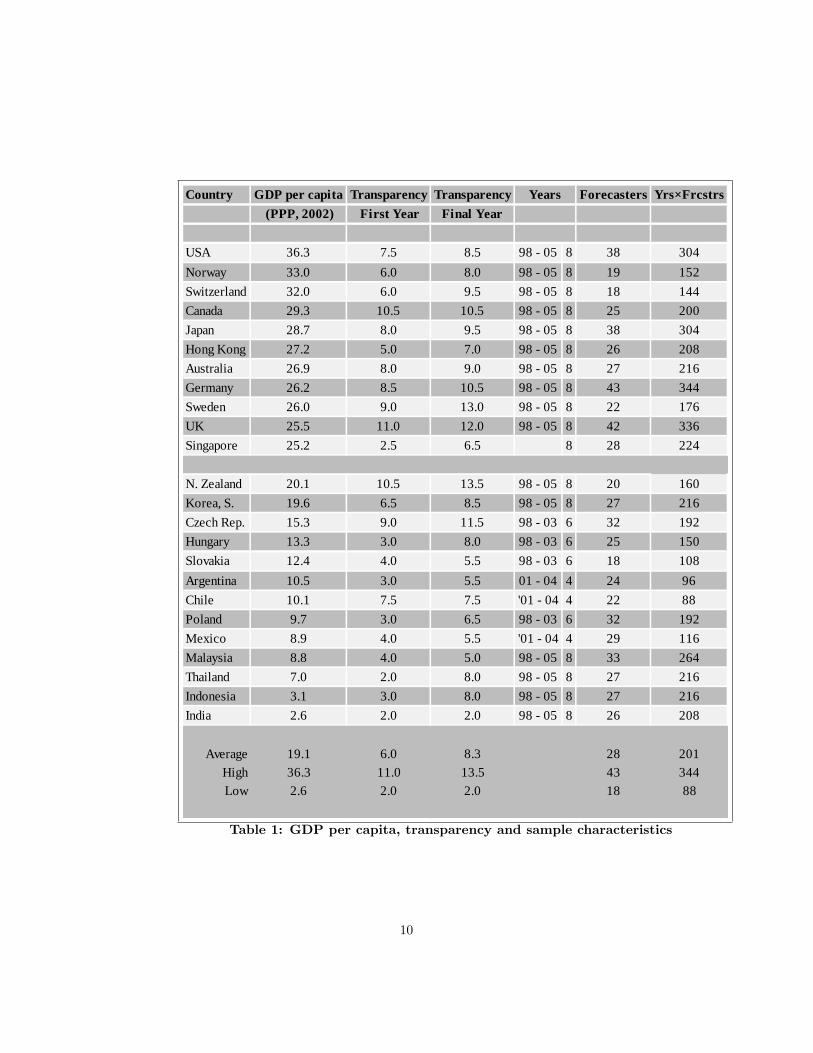
Country GDP per capita Transparency Transparency Forecasters Yrs×Frcstrs (PPP, 2002) First Year Final Year
USA 36.3 7.5 8.5 98 05 8 38 304Norway 33.0 6.0 8.0 98 05 8 19 152Switzerland 32.0 6.0 9.5 98 05 8 18 144Canada 29.3 10.5 10.5 98 05 8 25 200Japan 28.7 8.0 9.5 98 05 8 38 304Hong Kong 27.2 5.0 7.0 98 05 8 26 208Australia 26.9 8.0 9.0 98 05 8 27 216Germany 26.2 8.5 10.5 98 05 8 43 344Sweden 26.0 9.0 13.0 98 05 8 22 176UK 25.5 11.0 12.0 98 05 8 42 336Singapore 25.2 2.5 6.5 8 28 224
N. Zealand 20.1 10.5 13.5 98 05 8 20 160Korea, S. 19.6 6.5 8.5 98 05 8 27 216Czech Rep. 15.3 9.0 11.5 98 03 6 32 192Hungary 13.3 3.0 8.0 98 03 6 25 150Slovakia 12.4 4.0 5.5 98 03 6 18 108Argentina 10.5 3.0 5.5 01 04 4 24 96Chile 10.1 7.5 7.5 '01 04 4 22 88Poland 9.7 3.0 6.5 98 03 6 32 192Mexico 8.9 4.0 5.5 '01 04 4 29 116Malaysia 8.8 4.0 5.0 98 05 8 33 264Thailand 7.0 2.0 8.0 98 05 8 27 216Indonesia 3.1 3.0 8.0 98 05 8 27 216India 2.6 2.0 2.0 98 05 8 26 208
Average 19.1 6.0 8.3 28 201High 36.3 11.0 13.5 43 344Low 2.6 2.0 2.0 18 88
Years
Table 1: GDP per capita, transparency and sample characteristics
10
3.2 Professional forecasts error and interest rate volatility
Several sources are available for professional interest rate forecasts. Informa-tion services Bloomberg and Reuters conduct regular surveys of professionalforecasters as do central banks themselves, such as the Philadelphia FederalReserve and the ECB. Consensus Economics, however, surveys private sectoreconomic forecasters in a standardized way over a larger set of countries thanother sources.
Consensus Economics collects forecasts for short-term interest rates for avariety of countries, typically of a three month maturity, either from governmentbills, interbank rates or another benchmark rate. For some economies interestrate forecasts are unavailable or have a different maturity. These countries areexcluded from the sample. During the sample period, the three month maturityis short enough that it can be considered to be essentially driven by monetarypolicy and thus serves as the best available indicator of policy rates for whichforecasts are available for a wide set of countries.
Survey participants for a particular country are asked for their forecasts ofthe three month money market rate of that country for both three and twelvemonths in the future. More specifically, every month survey participants areasked for their interest rate forecasts for the end of the third subsequent calendarmonth and the end of the same calendar month in the following year. Forexample, the July 1999 survey presents forecasts for the end of October 1999and the end of July 2000.
Consensus Economics does not collect interest rate forecasts for the Euro-zone as a whole, but does so for several constituent countries. There is, however,only one interbank rate for the entire monetary union.4 Using several Euro-zonecountries in the panel would create multiple observations regarding only theEuropean Central Bank. Instead, I use forecasts for just Germany. Not only isGermany the largest economy in the Eurozone, it has by far the largest numberof forecasters.
The Consensus Economics data used are extracted from the hard copy book-lets at the Hong Kong Monetary Authority library. The “Eastern Europe Con-sensus Forecasts” were only available between 1998 and 2003 and the “LatinAmerican Consensus Forecasts”between 2001 and April 2004. Over the sam-ple the Consensus Economics surveys were conducted every month except forEastern Europe, for which the surveys were conducted every second month.The closing date for the survey ranges from 8th to 14th day of the month forindustrialized and Asia-Pacific countries and from the 15th to 21st for EasternEuropean and Latin American countries. To match the Dincer and Eichengreen(2007) data, I use the survey results only for the month closest to the middle
4Except for the three month forecasted in 1998, the year before the euro was introduced.
11
of the year. This is July in all cases except for Argentina, Chile and Mexico in2004 where I use April.
Forecasts are collected by individual organization per country. These includea variety of non-governmental entities such as independent or university affi li-ated research institutes and economic consulting firms. The majority, however,are financial institutions varying from domestic and regional commercial banksto global investment banks. There are 331 different organizations providingforecasts, with only 59 of these providing forecasts for more than one country.In the cross-section forecasters are treated separately per country (i.e. a Britishbank forecasting both the UK and the USA would count as two separate fore-casters) resulting in a total of 658. Because forecasters rarely provide forecastsfor all years, the sample contains only 2236 forecasts for three months aheadand 2191 forecasts for one year ahead.
To determine their accuracy, forecasts need to be compared to outcomesthree and twelve months down the road. To do so, data for the forecastedinterest rates were gathered from EcoWin, CEIC and Bloomberg. The absolutedifference between the individual forecast at t and the actual outcome at t +3 months and t + 12 months forms a direct measure of the accuracy of theindividual forecasts.
To measure the volatility of interest rates I calculate the standard deviationof interest rates using daily data for the three subsequent calendar months(typically first day of August until the last day of October) and the followingtwelve calendar months (typically first day of August to the last day of July thefollowing year). There are numerous forecasters per country, so the number ofindividual forecast errors (2236 and 2191, as above) greatly exceeds the numberof observations for the volatility measure (172).
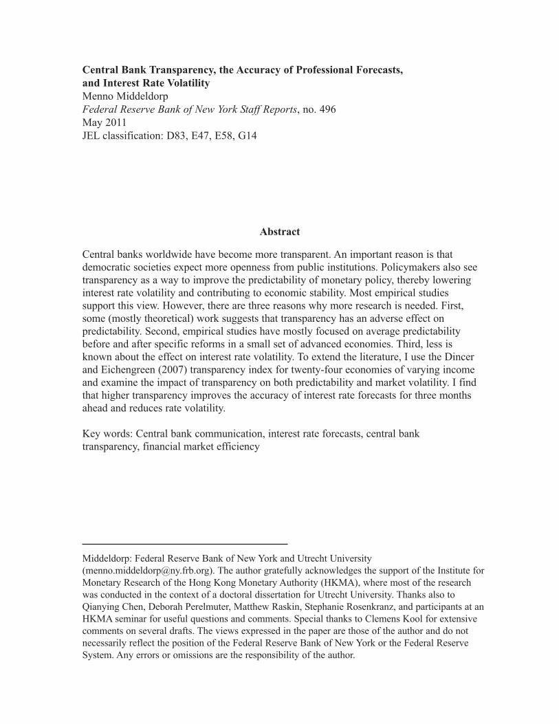
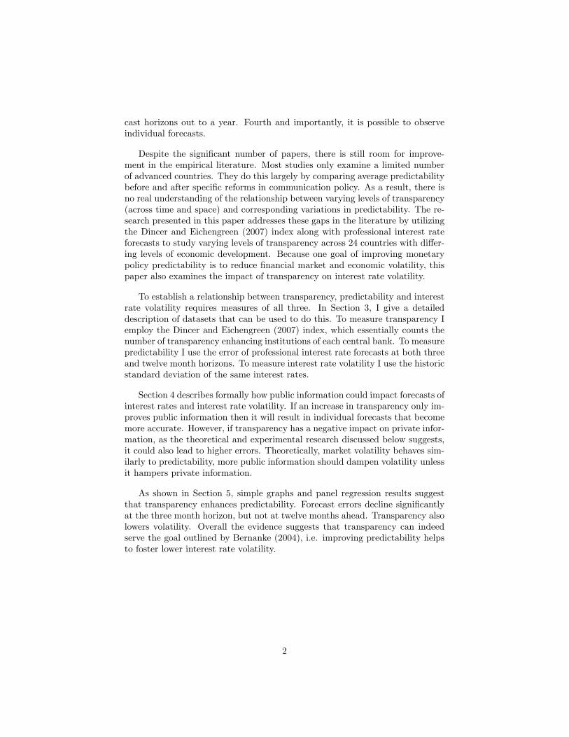
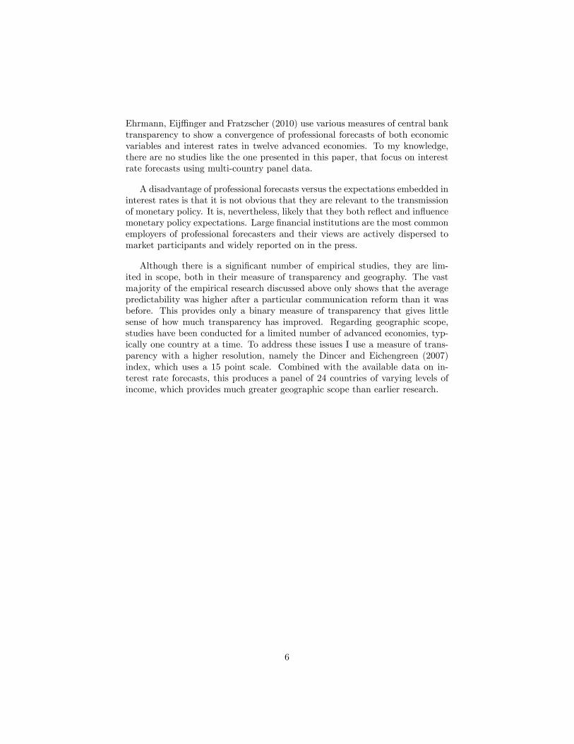
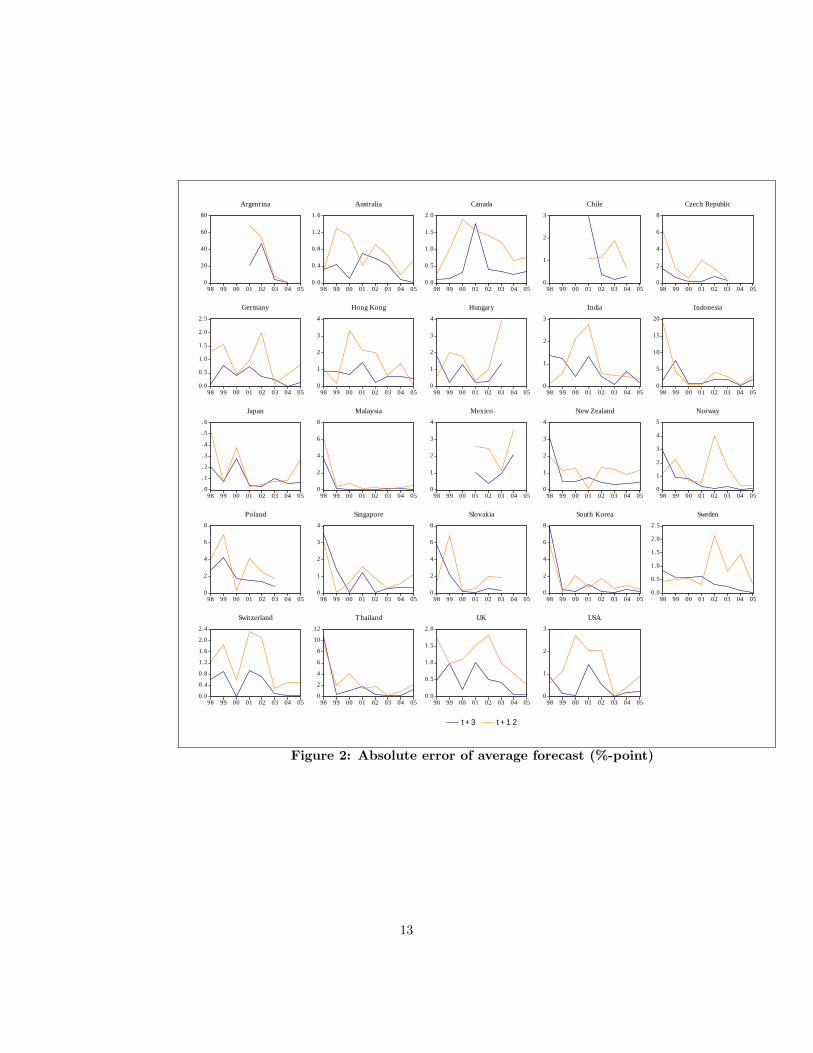
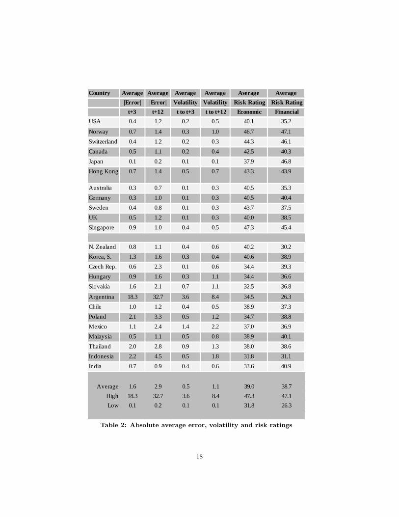
To graphically illustrate the general development of forecast errors per coun-try I also calculate the absolute difference between the average forecast (i.e. the“consensus” of forecasters) and the actual interest rate at t + 3 months andt + 12 months. Results are charted in Figure 2. As one might expect, the 3month errors are generally smaller than the 12 month errors. Errors and theirvariation are particularly large for countries that experienced financial and eco-nomic crisis during this period, Argentina in particular dramatically stands out.The 1998 financial market crisis affects several countries in the sample partic-ularly Asian and developing economies. The consequences of this shock varysubstantially, however, with peak errors varying from 0.5%-point for Japan to20%-point for Indonesia. The 2001 recession is also visible for a minority of ad-vanced economies. Overall, forecast errors vary substantially per country (alsosee Table 2) and show different variations over time.
12
0
20
40
60
80
98 99 00 01 02 03 04 05
Argentina
0.0
0.4
0.8
1.2
1.6
98 99 00 01 02 03 04 05
Australia
0.0
0.5
1.0
1.5
2.0
98 99 00 01 02 03 04 05
Canada
0
1
2
3
98 99 00 01 02 03 04 05
Chile
0
2
4
6
8
98 99 00 01 02 03 04 05
Czech Republic
0.0
0.5
1.0
1.5
2.0
2.5
98 99 00 01 02 03 04 05
Germany
0
1
2
3
4
98 99 00 01 02 03 04 05
Hong Kong
0
1
2
3
4
98 99 00 01 02 03 04 05
Hungary
0
1
2
3
98 99 00 01 02 03 04 05
India
0
5
10
15
20
98 99 00 01 02 03 04 05
Indonesia
. 0
.1
.2
.3
.4
.5
.6
98 99 00 01 02 03 04 05
Japan
0
2
4
6
8
98 99 00 01 02 03 04 05
Malaysia
0
1
2
3
4
98 99 00 01 02 03 04 05
Mexico
0
1
2
3
4
98 99 00 01 02 03 04 05
New Zealand
0
1
2
3
4
5
98 99 00 01 02 03 04 05
Norway
0
2
4
6
8
98 99 00 01 02 03 04 05
Poland
0
1
2
3
4
98 99 00 01 02 03 04 05
Singapore
0
2
4
6
8
98 99 00 01 02 03 04 05
Slovakia
0
2
4
6
8
98 99 00 01 02 03 04 05
South Korea
0.0
0.5
1.0
1.5
2.0
2.5
98 99 00 01 02 03 04 05
Sweden
0.0
0.4
0.8
1.2
1.6
2.0
2.4
98 99 00 01 02 03 04 05
Switzerland
0
2
4
6
8
10
12
98 99 00 01 02 03 04 05
Thailand
0.0
0.5
1.0
1.5
2.0
98 99 00 01 02 03 04 05
UK
0
1
2
3
98 99 00 01 02 03 04 05
t + 3 t + 1 2
USA
Figure 2: Absolute error of average forecast (%-point)
13
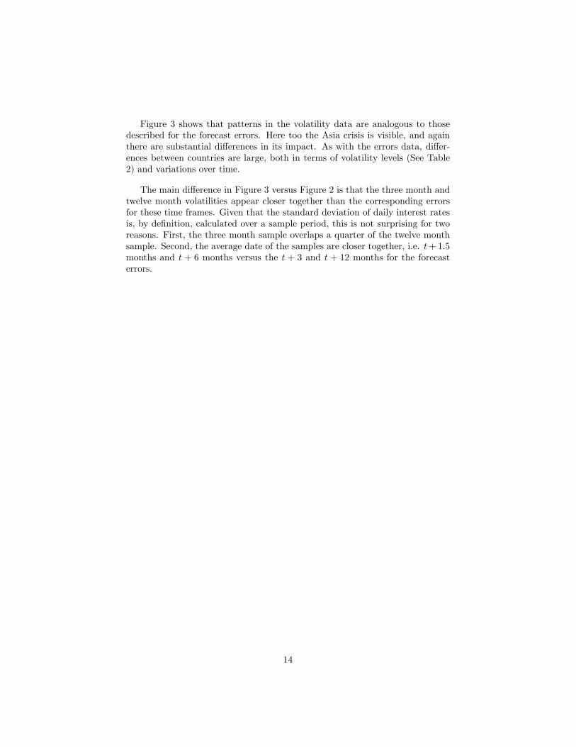
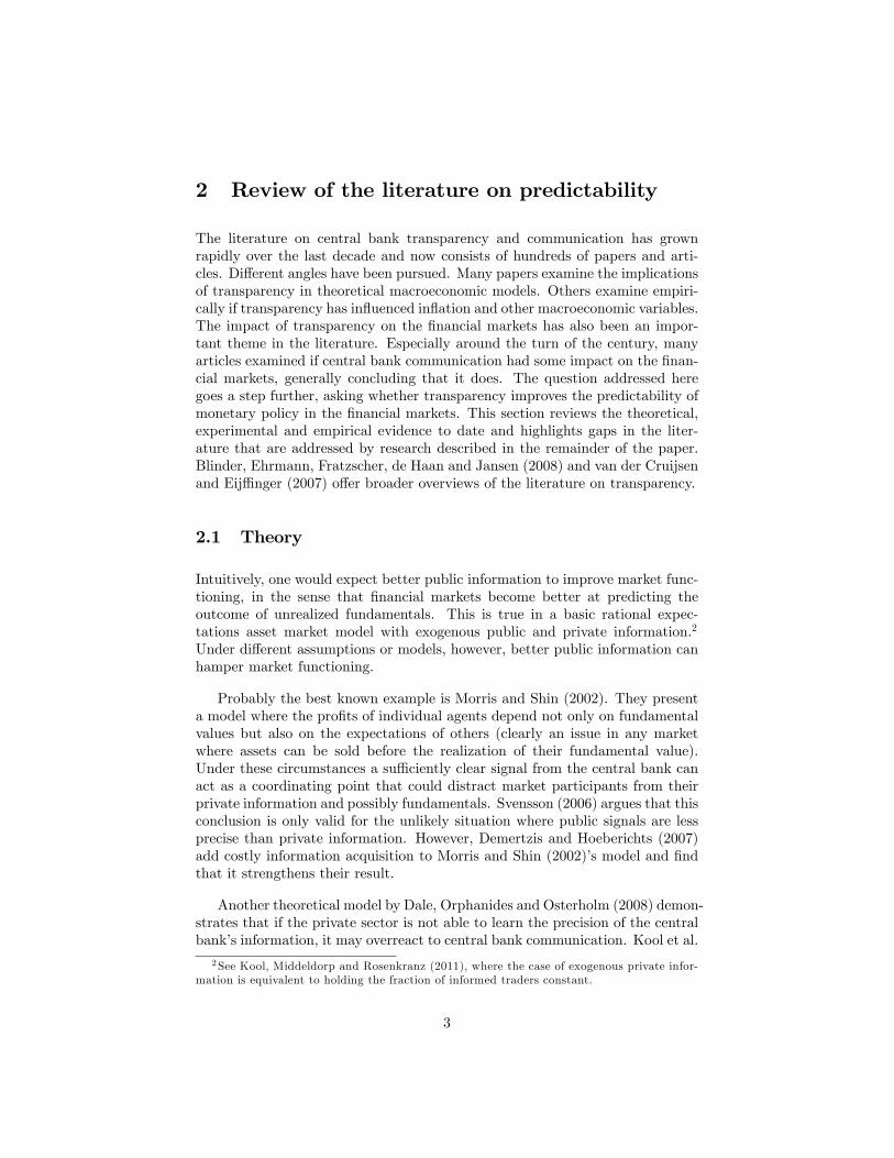
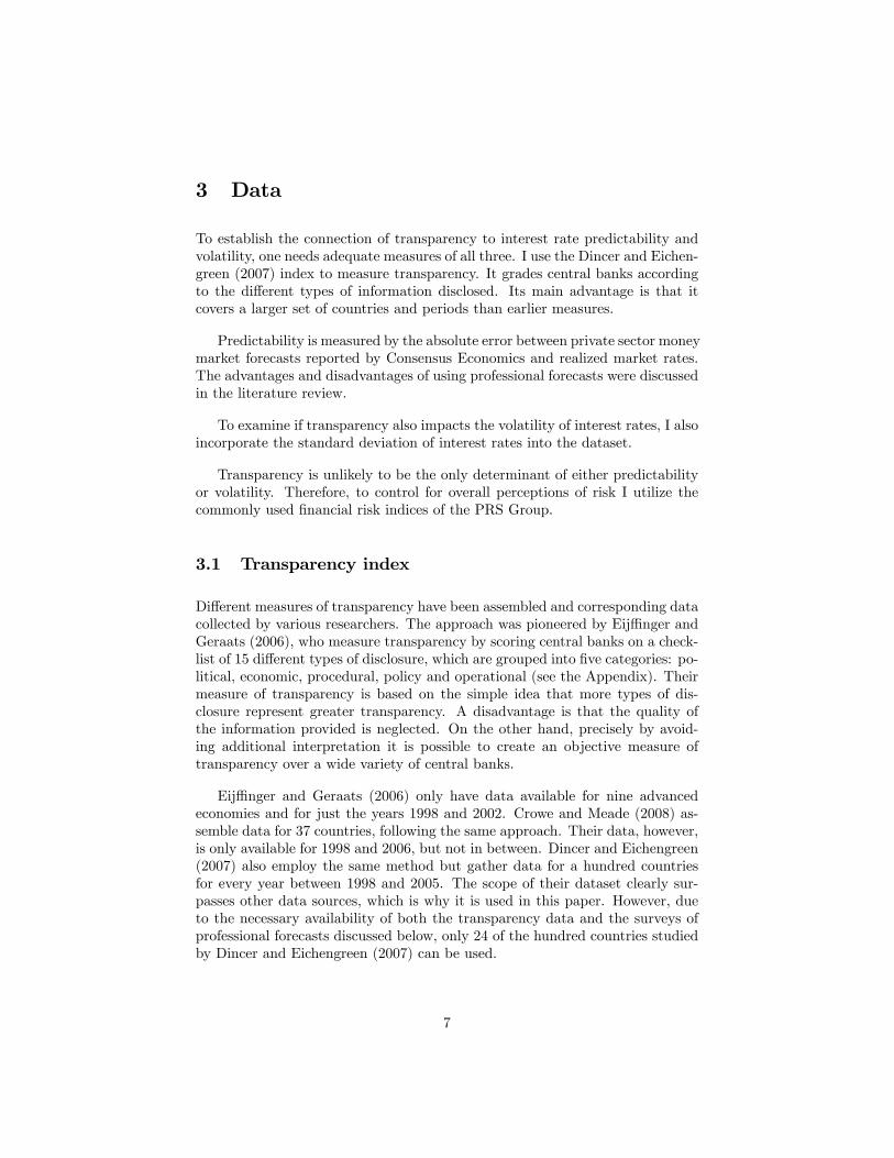
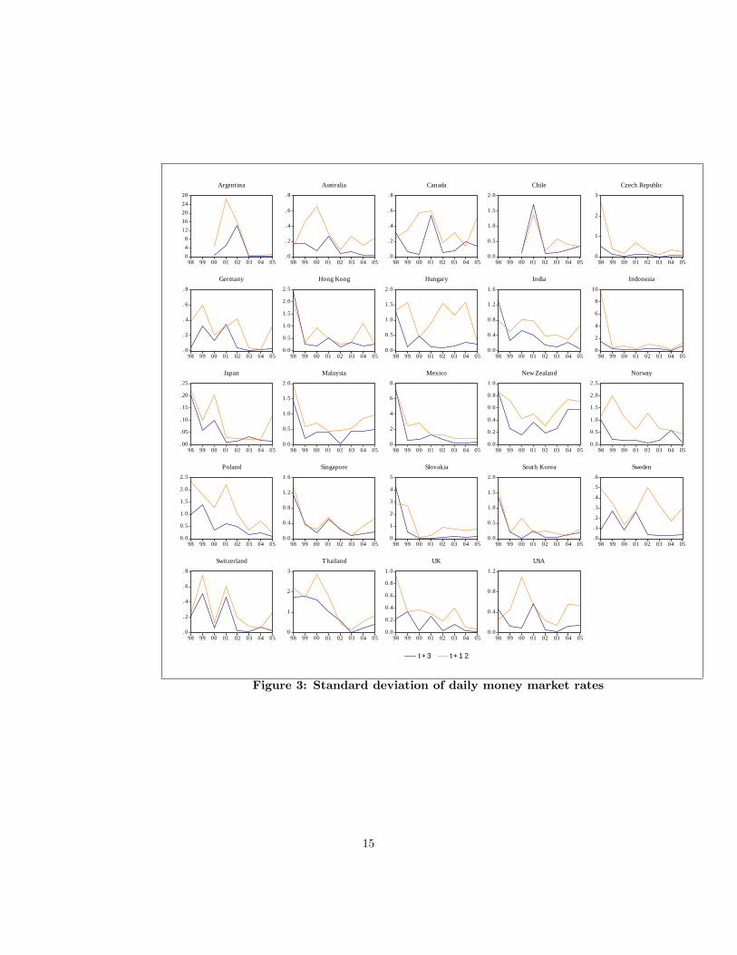
Figure 3 shows that patterns in the volatility data are analogous to thosedescribed for the forecast errors. Here too the Asia crisis is visible, and againthere are substantial differences in its impact. As with the errors data, differ-ences between countries are large, both in terms of volatility levels (See Table2) and variations over time.
The main difference in Figure 3 versus Figure 2 is that the three month andtwelve month volatilities appear closer together than the corresponding errorsfor these time frames. Given that the standard deviation of daily interest ratesis, by definition, calculated over a sample period, this is not surprising for tworeasons. First, the three month sample overlaps a quarter of the twelve monthsample. Second, the average date of the samples are closer together, i.e. t+ 1.5months and t + 6 months versus the t + 3 and t + 12 months for the forecasterrors.
14
048
1216202428
98 99 00 01 02 03 04 05
Argentina
. 0
.2
.4
.6
.8
98 99 00 01 02 03 04 05
Australia
. 0
.2
.4
.6
.8
98 99 00 01 02 03 04 05
Canada
0.0
0.5
1.0
1.5
2.0
98 99 00 01 02 03 04 05
Chile
0
1
2
3
98 99 00 01 02 03 04 05
Czech Republic
. 0
.2
.4
.6
.8
98 99 00 01 02 03 04 05
Germany
0.0
0.5
1.0
1.5
2.0
2.5
98 99 00 01 02 03 04 05
Hong Kong
0.0
0.5
1.0
1.5
2.0
98 99 00 01 02 03 04 05
Hungary
0.0
0.4
0.8
1.2
1.6
98 99 00 01 02 03 04 05
India
0
2
4
6
8
10
98 99 00 01 02 03 04 05
Indonesia
. 00
.05
.10
.15
.20
.25
98 99 00 01 02 03 04 05
Japan
0.0
0.5
1.0
1.5
2.0
98 99 00 01 02 03 04 05
Malaysia
0
2
4
6
8
98 99 00 01 02 03 04 05
Mexico
0.0
0.2
0.4
0.6
0.8
1.0
98 99 00 01 02 03 04 05
New Zealand
0.0
0.5
1.0
1.5
2.0
2.5
98 99 00 01 02 03 04 05
Norway
0.0
0.5
1.0
1.5
2.0
2.5
98 99 00 01 02 03 04 05
Poland
0.0
0.4
0.8
1.2
1.6
98 99 00 01 02 03 04 05
Singapore
0
1
2
3
4
5
98 99 00 01 02 03 04 05
Slovakia
0.0
0.5
1.0
1.5
2.0
98 99 00 01 02 03 04 05
South Korea
. 0
.1
.2
.3
.4
.5
.6
98 99 00 01 02 03 04 05
Sweden
. 0
.2
.4
.6
.8
98 99 00 01 02 03 04 05
Switzerland
0
1
2
3
98 99 00 01 02 03 04 05
Thailand
0.0
0.2
0.4
0.6
0.8
1.0
98 99 00 01 02 03 04 05
UK
0.0
0.4
0.8
1.2
98 99 00 01 02 03 04 05
t + 3 t + 1 2
USA
Figure 3: Standard deviation of daily money market rates
15
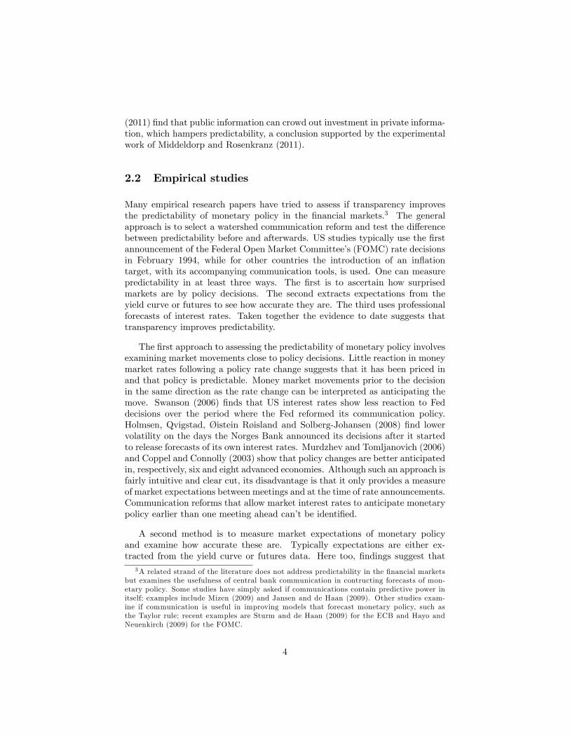
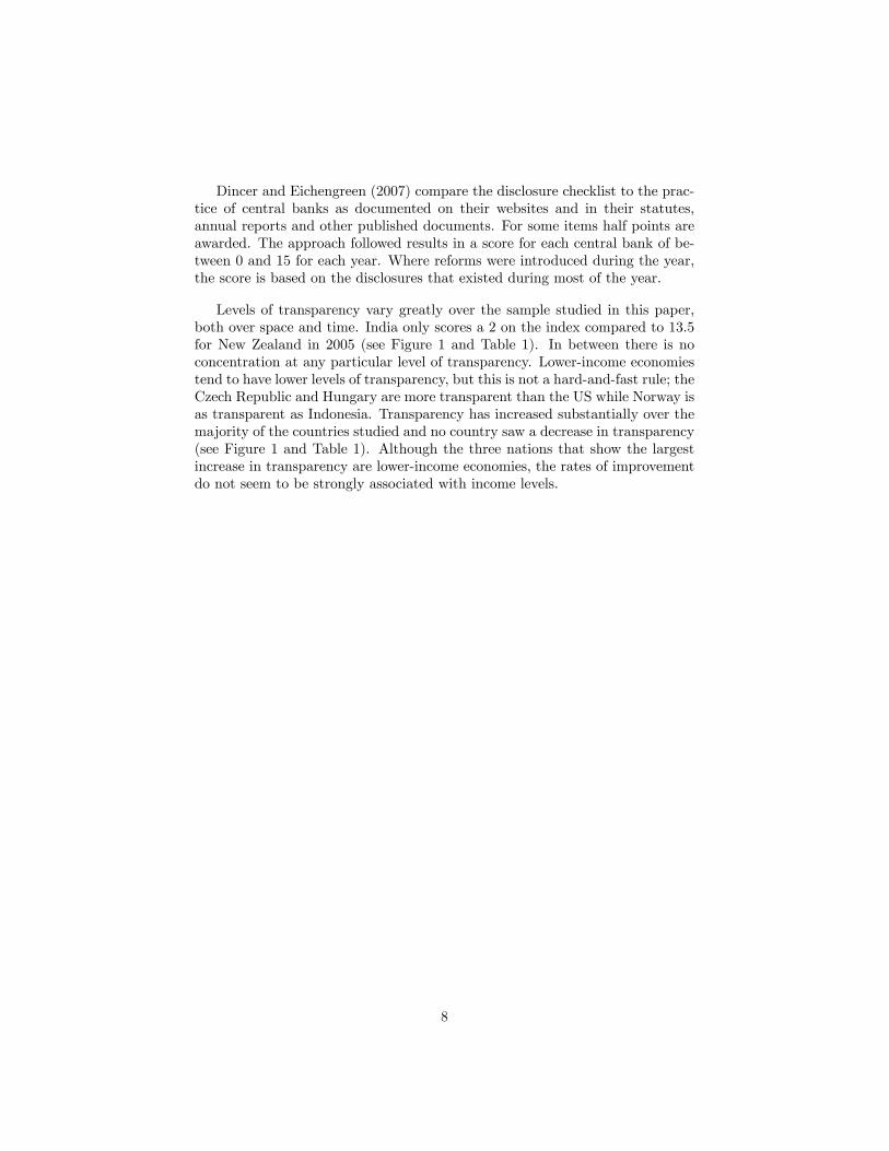
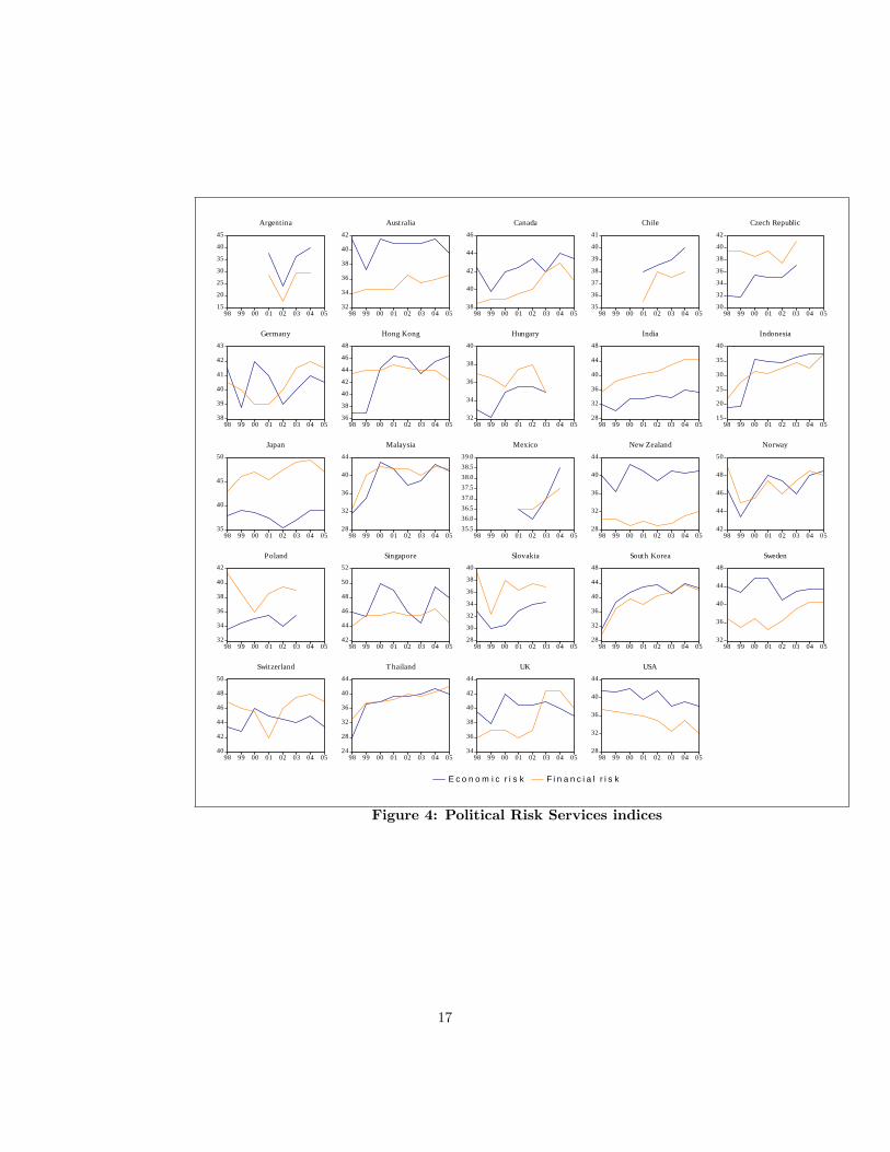
Forecast errors and financial market volatility reflect more than just thetransparency of the central bank. Both are affected by overall predictability ofinterest rates due to the economic and financial risks that affect them. To controlfor country risk in the analysis below, I utilize the economic and financial riskindicators of the International Country Risk Guide of the Political Risk Services(PRS) Group. According to Linder and Santiso (2002) these ratings are usedby around four-fifths of the companies on Fortune magazine’s list of largestmultinationals. The financial and economics risk ratings are constructed withobjective data that are weighed together according to predefined scales.5 Higherratings indicate less risk. The economic risk rating is constructed from GDP perhead, real GDP growth, inflation, general government balance as a percentage ofGDP and current account as a percentage of GDP. The components of financialrisk are foreign debt as a percentage of GDP, foreign debt service as a percentageof exports of goods and services, current account as percentage of exports ofgoods and services, offi cial reserves import cover and year-on-year exchange ratemovement. Essentially the risk ratings provide a standardized and parsimoniousway to reflect a variety of economic and financial fundamentals that affect risk.A downside may be that the ratings may not reflect differences in the abilityof countries to maintain government and current account deficits or carry debt,see for example the relatively low ratings of some developed countries in Figure4 and Table 2.
5See http://www.prsgroup.com/PDFS/icrgmethodology.pdf.
16
15
20
25
30
35
40
45
98 99 00 01 02 03 04 05
Argentina
32
34
36
38
40
42
98 99 00 01 02 03 04 05
Australia
38
40
42
44
46
98 99 00 01 02 03 04 05
Canada
35
36
37
38
39
40
41
98 99 00 01 02 03 04 05
Chile
30
32
34
36
38
40
42
98 99 00 01 02 03 04 05
Czech Republic
38
39
40
41
42
43
98 99 00 01 02 03 04 05
Germany
36
38
40
42
44
46
48
98 99 00 01 02 03 04 05
Hong Kong
32
34
36
38
40
98 99 00 01 02 03 04 05
Hungary
28
32
36
40
44
48
98 99 00 01 02 03 04 05
India
15
20
25
30
35
40
98 99 00 01 02 03 04 05
Indonesia
35
40
45
50
98 99 00 01 02 03 04 05
Japan
28
32
36
40
44
98 99 00 01 02 03 04 05
Malaysia
35.536.036.537.037.538.038.539.0
98 99 00 01 02 03 04 05
Mexico
28
32
36
40
44
98 99 00 01 02 03 04 05
New Zealand
42
44
46
48
50
98 99 00 01 02 03 04 05
Norway
32
34
36
38
40
42
98 99 00 01 02 03 04 05
Poland
42
44
46
48
50
52
98 99 00 01 02 03 04 05
Singapore
28
30
32
34
36
38
40
98 99 00 01 02 03 04 05
Slovakia
28
32
36
40
44
48
98 99 00 01 02 03 04 05
South Korea
32
36
40
44
48
98 99 00 01 02 03 04 05
Sweden
40
42
44
46
48
50
98 99 00 01 02 03 04 05
Switzerland
24
28
32
36
40
44
98 99 00 01 02 03 04 05
T hailand
34
36
38
40
42
44
98 99 00 01 02 03 04 05
UK
28
32
36
40
44
98 99 00 01 02 03 04 05
E c o n o m i c r i s k F i n a n c i a l r i s k
USA
Figure 4: Political Risk Services indices
17
Country Average Average Average Average Average Average|Error| |Error| Volatility Volatility Risk Rating Risk Rating
t+3 t+12 t to t+3 t to t+12 Economic FinancialUSA 0.4 1.2 0.2 0.5 40.1 35.2
Norway 0.7 1.4 0.3 1.0 46.7 47.1Switzerland 0.4 1.2 0.2 0.3 44.3 46.1Canada 0.5 1.1 0.2 0.4 42.5 40.3Japan 0.1 0.2 0.1 0.1 37.9 46.8Hong Kong 0.7 1.4 0.5 0.7 43.3 43.9
Australia 0.3 0.7 0.1 0.3 40.5 35.3Germany 0.3 1.0 0.1 0.3 40.5 40.4Sweden 0.4 0.8 0.1 0.3 43.7 37.5UK 0.5 1.2 0.1 0.3 40.0 38.5Singapore 0.9 1.0 0.4 0.5 47.3 45.4
N. Zealand 0.8 1.1 0.4 0.6 40.2 30.2Korea, S. 1.3 1.6 0.3 0.4 40.6 38.9Czech Rep. 0.6 2.3 0.1 0.6 34.4 39.3Hungary 0.9 1.6 0.3 1.1 34.4 36.6Slovakia 1.6 2.1 0.7 1.1 32.5 36.8
Argentina 18.3 32.7 3.6 8.4 34.5 26.3Chile 1.0 1.2 0.4 0.5 38.9 37.3Poland 2.1 3.3 0.5 1.2 34.7 38.8Mexico 1.1 2.4 1.4 2.2 37.0 36.9Malaysia 0.5 1.1 0.5 0.8 38.9 40.1Thailand 2.0 2.8 0.9 1.3 38.0 38.6Indonesia 2.2 4.5 0.5 1.8 31.8 31.1India 0.7 0.9 0.4 0.6 33.6 40.9
Average 1.6 2.9 0.5 1.1 39.0 38.7High 18.3 32.7 3.6 8.4 47.3 47.1Low 0.1 0.2 0.1 0.1 31.8 26.3
Table 2: Absolute average error, volatility and risk ratings
18
4 A simple theoretical approach to public andprivate information
Here I describe how transparency might have either a positive or negative effecton predictability in a very general but formal way. Along the lines of the datasetemployed below, consider a number of central banks, each with an accompanyingset of professional forecasters who make predictions of future policy rates.
A simple way to think about individual forecasts is as combinations of publicand private information, which are both noisy signals of future policy rates.The noise in the signals are random errors that are assumed to be unbiasedand independently normally distributed. In the context of the data used, thesesignals have a year index, t, but I suppress the subscript in this section becauseit applies to all variables.
(1) yk = bk + ωk ωk = N(
0, 1√∆k
)Where
y public signalb future policy rateωk error of public signal for country kk country index∆ precision of public signal error (i.e. inverse of the variance)
(2) pi,k = bk + ωi,k ωi,k = N(
0, 1√si,k
)Where
pi,k private signal of forecaster i for country ki forecaster indexωi,k error of private signal of forecaster i for country ksi,k precision of private signal error (i.e. inverse of the variance)
Assuming the forecaster aims to maximize accuracy, knows the precisions ofthe public and private signals, and behaves rationally, the individual forecast,fi,k, will be a combination of private and public signals, using relative precisionsas weights.
(3) fi,k = ∆k
∆k+si,ky +
si,k∆+si,k
pi,k
The error of the individual forecast with the future interest rate, ξi,k , isderived by subtracting b from the forecast.
19
(4) ξi,k = fi,k − bk = ∆k
∆k+si,kωk +
si,k∆+si,k
ωi,k
A convenient property of signals with normally and independently distrib-uted errors is that the combined signal has a precision that is the sum of theprecisions of the individual signals. Equation (5) thus represents the precisionof the forecast error, ζi,k.
(5) ζi,k = ∆k + si,k
It seems likely that transparency will increase the precision of the publicinformation. Equation (6) defines ∆k to be a function of transparency (τ) andsome other determinants Dk.
(6) ∆k = φ∆ (+τ ,Dk)
Where
τ transparencyDk vector of other determinants of the precision of public information
It is less clear if transparency will affect private information. In Equation(4) the weight on public information will increase as it becomes more preciseand the weight on private information will decline, while the precision of privateinformation will remain unchanged. It may be the case, however, that the preci-sion itself is also affected. In line with the reasoning of Morris and Shin (2002),agents may partially ignore their own private information because the publicsignal acts as a coordinator of second degree expectations and thus becomesover-emphasized in determining the resale value of the asset. Kool et al. (2011)also raise the possibility that when private information is costly individual fore-casters will invest less in the precision of the private signal. Both cases imply anegative relationship between transparency and private information.
(7) si,k = φs (−τ ,Di,k)
As a result, the relationship between transparency and predictability will bea function of transparency’s separate effects on the public and private signals.
(8) ζi,k = φ∆ (+τ ,Dk) + φs (−τ ,Di,k)
Kool et al. (2011) show that in a rational expectations asset market theaffect of transparency on volatility is theoretically the same as its affect onpredictability. They show that transparency can crowd out private informationand thereby both hurt predictability and push up volatility.
It is quite possible that in order to closely model the relationship betweentransparency and the precisions of private and public information a more com-plex setup would be required. For example, to represent the idea of Dale et al.(2008) that forecasters may misestimate the precision of the public signal would
20
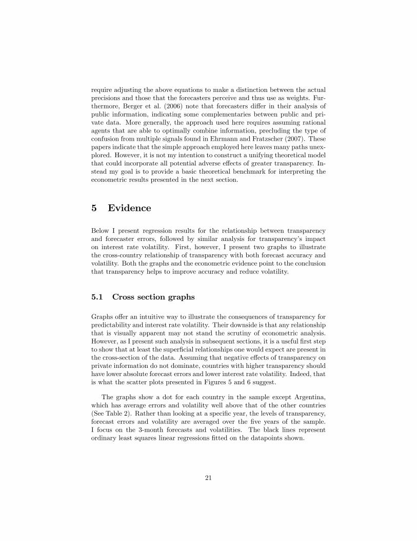
require adjusting the above equations to make a distinction between the actualprecisions and those that the forecasters perceive and thus use as weights. Fur-thermore, Berger et al. (2006) note that forecasters differ in their analysis ofpublic information, indicating some complementaries between public and pri-vate data. More generally, the approach used here requires assuming rationalagents that are able to optimally combine information, precluding the type ofconfusion from multiple signals found in Ehrmann and Fratzscher (2007). Thesepapers indicate that the simple approach employed here leaves many paths unex-plored. However, it is not my intention to construct a unifying theoretical modelthat could incorporate all potential adverse effects of greater transparency. In-stead my goal is to provide a basic theoretical benchmark for interpreting theeconometric results presented in the next section.
5 Evidence
Below I present regression results for the relationship between transparencyand forecaster errors, followed by similar analysis for transparency’s impacton interest rate volatility. First, however, I present two graphs to illustratethe cross-country relationship of transparency with both forecast accuracy andvolatility. Both the graphs and the econometric evidence point to the conclusionthat transparency helps to improve accuracy and reduce volatility.
5.1 Cross section graphs
Graphs offer an intuitive way to illustrate the consequences of transparency forpredictability and interest rate volatility. Their downside is that any relationshipthat is visually apparent may not stand the scrutiny of econometric analysis.However, as I present such analysis in subsequent sections, it is a useful first stepto show that at least the superficial relationships one would expect are present inthe cross-section of the data. Assuming that negative effects of transparency onprivate information do not dominate, countries with higher transparency shouldhave lower absolute forecast errors and lower interest rate volatility. Indeed, thatis what the scatter plots presented in Figures 5 and 6 suggest.
The graphs show a dot for each country in the sample except Argentina,which has average errors and volatility well above that of the other countries(See Table 2). Rather than looking at a specific year, the levels of transparency,forecast errors and volatility are averaged over the five years of the sample.I focus on the 3-month forecasts and volatilities. The black lines representordinary least squares linear regressions fitted on the datapoints shown.
21
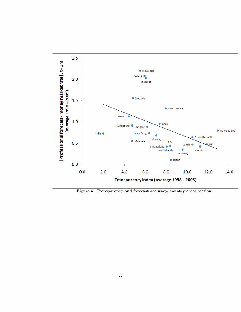
Figure 5: Transparency and forecast accuracy, country cross section
22
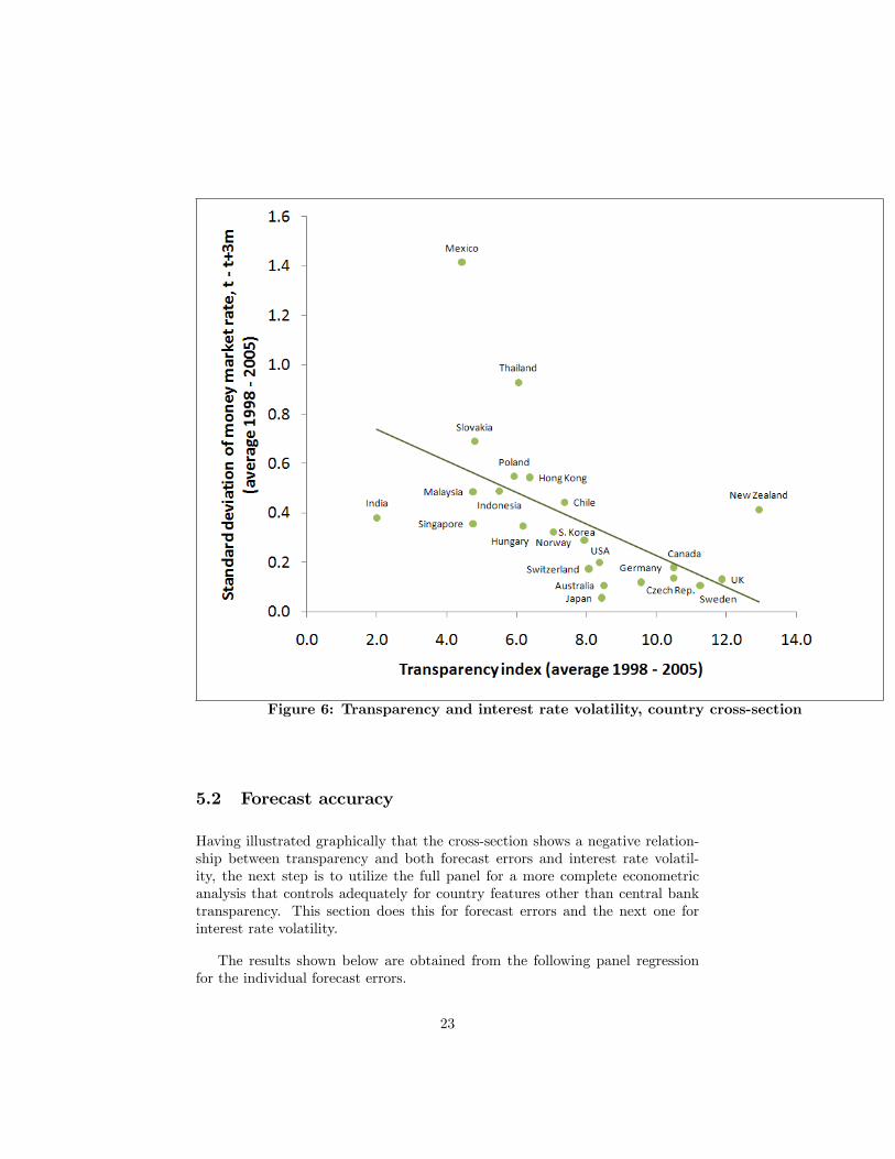
Figure 6: Transparency and interest rate volatility, country cross-section
5.2 Forecast accuracy
Having illustrated graphically that the cross-section shows a negative relation-ship between transparency and both forecast errors and interest rate volatil-ity, the next step is to utilize the full panel for a more complete econometricanalysis that controls adequately for country features other than central banktransparency. This section does this for forecast errors and the next one forinterest rate volatility.
The results shown below are obtained from the following panel regressionfor the individual forecast errors.
23
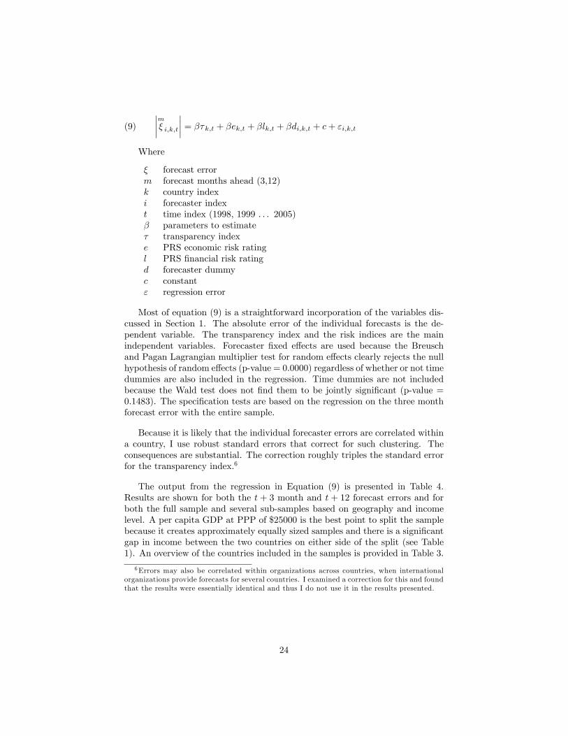
(9)
∣∣∣∣mξ i,k,t∣∣∣∣ = βτk,t + βek,t + βlk,t + βdi,k,t + c+ εi,k,t
Where
ξ forecast errorm forecast months ahead (3,12)k country indexi forecaster indext time index (1998, 1999 . . . 2005)β parameters to estimateτ transparency indexe PRS economic risk ratingl PRS financial risk ratingd forecaster dummyc constantε regression error
Most of equation (9) is a straightforward incorporation of the variables dis-cussed in Section 1. The absolute error of the individual forecasts is the de-pendent variable. The transparency index and the risk indices are the mainindependent variables. Forecaster fixed effects are used because the Breuschand Pagan Lagrangian multiplier test for random effects clearly rejects the nullhypothesis of random effects (p-value = 0.0000) regardless of whether or not timedummies are also included in the regression. Time dummies are not includedbecause the Wald test does not find them to be jointly significant (p-value =0.1483). The specification tests are based on the regression on the three monthforecast error with the entire sample.
Because it is likely that the individual forecaster errors are correlated withina country, I use robust standard errors that correct for such clustering. Theconsequences are substantial. The correction roughly triples the standard errorfor the transparency index.6
The output from the regression in Equation (9) is presented in Table 4.Results are shown for both the t + 3 month and t + 12 forecast errors and forboth the full sample and several sub-samples based on geography and incomelevel. A per capita GDP at PPP of $25000 is the best point to split the samplebecause it creates approximately equally sized samples and there is a significantgap in income between the two countries on either side of the split (see Table1). An overview of the countries included in the samples is provided in Table 3.
6Errors may also be correlated within organizations across countries, when internationalorganizations provide forecasts for several countries. I examined a correction for this and foundthat the results were essentially identical and thus I do not use it in the results presented.
24
GDP per capita > $25k GDP per capita < $25kAsiaPacific Australia, Hong Kong,
Japan, SingaporeIndia, Indonesia, Malaysia, N.Zealand, S. Korea, Thailand
Europe Germany, Norway, Sweden,Switzerland, UK
Czech Republic, Hungary,Poland, Slovakia
Americas Canada, USA Argentina, Chile, Mexico
Table 3: Sample matrix
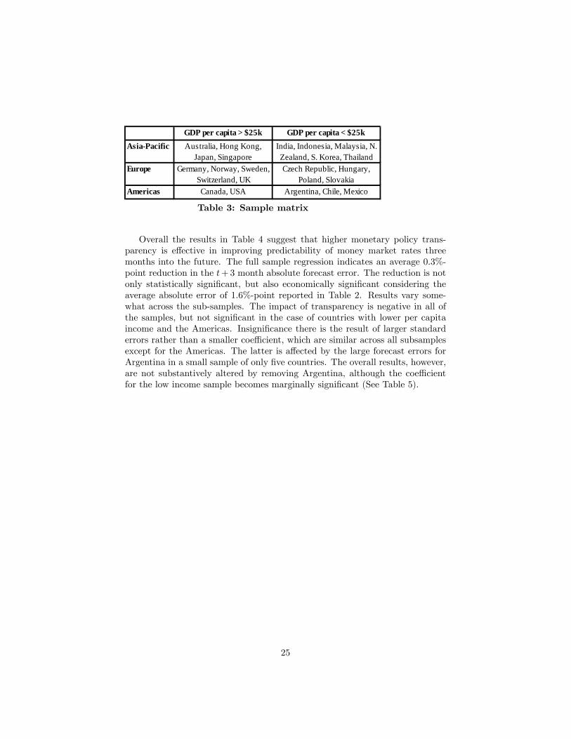
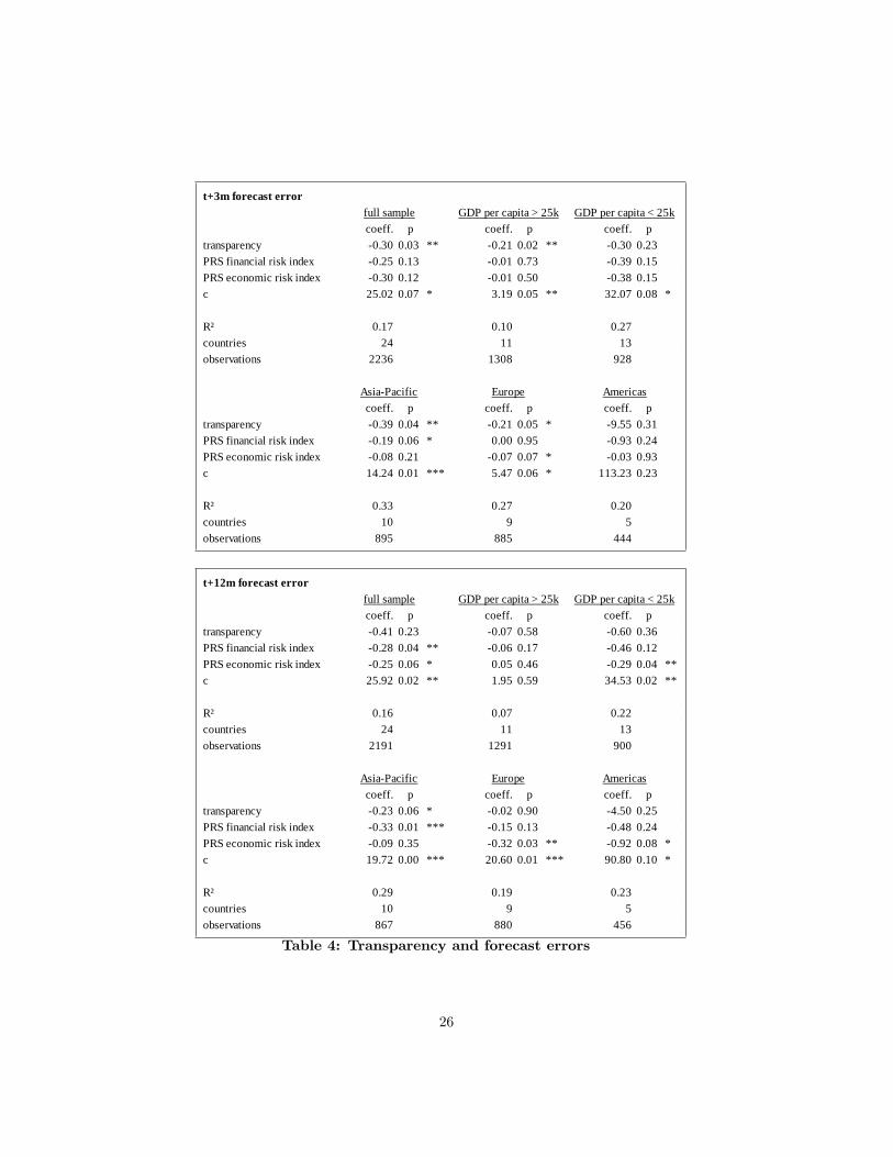
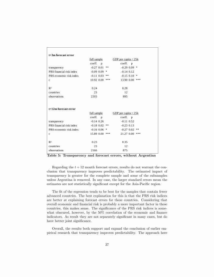
Overall the results in Table 4 suggest that higher monetary policy trans-parency is effective in improving predictability of money market rates threemonths into the future. The full sample regression indicates an average 0.3%-point reduction in the t+ 3 month absolute forecast error. The reduction is notonly statistically significant, but also economically significant considering theaverage absolute error of 1.6%-point reported in Table 2. Results vary some-what across the sub-samples. The impact of transparency is negative in all ofthe samples, but not significant in the case of countries with lower per capitaincome and the Americas. Insignificance there is the result of larger standarderrors rather than a smaller coeffi cient, which are similar across all subsamplesexcept for the Americas. The latter is affected by the large forecast errors forArgentina in a small sample of only five countries. The overall results, however,are not substantively altered by removing Argentina, although the coeffi cientfor the low income sample becomes marginally significant (See Table 5).
25
t+3m forecast error
coeff. p coeff. p coeff. ptransparency 0.30 0.03 ** 0.21 0.02 ** 0.30 0.23PRS financial risk index 0.25 0.13 0.01 0.73 0.39 0.15PRS economic risk index 0.30 0.12 0.01 0.50 0.38 0.15c 25.02 0.07 * 3.19 0.05 ** 32.07 0.08 *
R² 0.17 0.10 0.27countries 24 11 13observations 2236 1308 928
coeff. p coeff. p coeff. ptransparency 0.39 0.04 ** 0.21 0.05 * 9.55 0.31PRS financial risk index 0.19 0.06 * 0.00 0.95 0.93 0.24PRS economic risk index 0.08 0.21 0.07 0.07 * 0.03 0.93c 14.24 0.01 *** 5.47 0.06 * 113.23 0.23
R² 0.33 0.27 0.20countries 10 9 5observations 895 885 444
full sample GDP per capita > 25k GDP per capita < 25k
AmericasEuropeAsiaPacific
t+12m forecast error
coeff. p coeff. p coeff. ptransparency 0.41 0.23 0.07 0.58 0.60 0.36PRS financial risk index 0.28 0.04 ** 0.06 0.17 0.46 0.12PRS economic risk index 0.25 0.06 * 0.05 0.46 0.29 0.04 **c 25.92 0.02 ** 1.95 0.59 34.53 0.02 **
R² 0.16 0.07 0.22countries 24 11 13observations 2191 1291 900
coeff. p coeff. p coeff. ptransparency 0.23 0.06 * 0.02 0.90 4.50 0.25PRS financial risk index 0.33 0.01 *** 0.15 0.13 0.48 0.24PRS economic risk index 0.09 0.35 0.32 0.03 ** 0.92 0.08 *c 19.72 0.00 *** 20.60 0.01 *** 90.80 0.10 *
R² 0.29 0.19 0.23countries 10 9 5observations 867 880 456
full sample GDP per capita > 25k GDP per capita < 25k
AmericasEuropeAsiaPacific
Table 4: Transparency and forecast errors
26
t+3m forecast error
coeff. p coeff. ptransparency 0.27 0.01 ** 0.29 0.09 *PRS financial risk index 0.09 0.09 * 0.14 0.12PRS economic risk index 0.11 0.03 ** 0.15 0.10 *c 10.92 0.00 *** 13.90 0.00 ***
R² 0.24 0.28countries 23 12observations 2203 895
t+12m forecast error
coeff. p coeff. ptransparency 0.14 0.26 0.11 0.52PRS financial risk index 0.18 0.02 ** 0.23 0.13PRS economic risk index 0.16 0.06 * 0.27 0.02 **c 15.89 0.00 *** 21.27 0.00 ***
R² 0.23 0.35countries 23 12observations 2166 875
full sample GDP per capita < 25k
full sample GDP per capita < 25k
Table 5: Transparency and forecast errors, without Argentina
Regarding the t+ 12 month forecast errors, results do not warrant the con-clusion that transparency improves predictability. The estimated impact oftransparency is greater for the complete sample and some of the subsamplesunless Argentina is removed. In any case, the larger standard errors mean theestimates are not statistically significant except for the Asia-Pacific region.
The fit of the regression tends to be best for the samples that contain feweradvanced countries. The best explanation for this is that the PRS risk indicesare better at explaining forecast errors for these countries. Considering thatoverall economic and financial risk is probably a more important factor in thesecountries, this makes sense. The significance of the PRS risk indices is some-what obscured, however, by the 50% correlation of the economic and financeindicators. As result they are not separately significant in many cases, but dohave better joint significance.
Overall, the results both support and expand the conclusion of earlier em-pirical research that transparency improves predictability. The approach here
27
improves on earlier research by actually measuring the relationship between atransparency index and predictability, so that it is possible to say how muchtransparency leads to how much predictability. It adds to the robustness of theconclusion by confirming it across a variety of countries. Although the effectis only weakly significant for the low income sample without Argentina, theconsistency of the coeffi cient suggests that it does apply to most countries, butcannot be established as strongly significant due to the larger standard errors.
The difference between transparency’s effect on predictability on the threemonth and twelve month forecast horizons suggests potential limits to the ben-efits of transparency. It seems plausible that any information asymmetries be-tween policy makers and professional forecasters are likely to be greatest in theshort term where the former group has, at the very least, a unique insight intotheir own views about incoming data and the economic outlook. As I find,greater transparency thus has more potential to improve the precision of publicinformation at shorter timeframes. At longer forecast horizons such informa-tion asymmetries are less obvious as the economic future becomes cloudier forall. It is thus not surprising to find that evidence of improved transparencyat the twelve month forecast horizon is very weak and inconsistent across sam-ples. It is possible, however, that there is some scope for central banks to shareinformation about the longer term outlook that has not been fully utilized.
5.3 Interest rate volatility
A potential benefit of improved monetary policy predictability is that it maylead to lower interest rate volatility. To examine the connection between trans-parency and interest rate volatility, I conduct a similar panel regression analysiswith interest rate volatility.
(10)∣∣∣mσk,t∣∣∣ = βτk,t + βek,t + βlk,t + βdk,t + c+ εi,k,t
Where
σ standard deviation of daily money market rates, from t to t+m
While the dependent variable is now a measure of interest rate volatility,the independent variables in Equation (10) are the same as in Equation (9). Asabove, the Breusch and Pagan test rejects the random effects specification, bothwith and without time fixed effects (p-value of 0.0068 and 0.0085 respectively).The Wald test rejects the joint significance of the time dummies (p-value of0.1345), so no time fixed effects are included.
28
t+3m daily standard deviation of 3m interest rate
coeff. p coeff. p coeff. ptransparency 0.11 0.10 0.12 0.00 *** 0.13 0.26PRS financial risk index 0.08 0.23 0.01 0.58 0.14 0.21PRS economic risk index 0.09 0.12 0.05 0.25 0.06 0.45c 7.97 0.04 ** 2.81 0.10 8.89 0.05 *
R² 0.51 0.39 0.50countries 24 11 13observations 172 88 84
coeff. p coeff. p coeff. ptransparency 0.14 0.00 *** 0.14 0.02 ** 1.75 0.00 ***PRS financial risk index 0.04 0.24 0.06 0.29 0.24 0.18PRS economic risk index 0.01 0.61 0.00 0.91 0.33 0.06 *c 3.50 0.00 *** 0.96 0.74 36.08 0.00 ***
R² 0.55 0.27 0.91countries 10 9 5observations 80 64 28
full sample GDP per capita > 25k GDP per capita < 25k
AsiaPacific Europe Americas
t+12m daily standard deviation of 3m interest rate
coeff. p coeff. p coeff. ptransparency 0.32 0.14 0.10 0.01 ** 0.13 0.26PRS financial risk index 0.09 0.24 0.03 0.10 0.14 0.21PRS economic risk index 0.09 0.31 0.05 0.16 0.06 0.45c 10.68 0.02 ** 4.48 0.01 *** 8.89 0.05 *
R² 0.51 0.52 0.50countries 24 11 13observations 172 88 84
coeff. p coeff. p coeff. ptransparency 0.32 0.14 0.10 0.01 ** 0.49 0.21PRS financial risk index 0.12 0.13 0.02 0.62 0.51 0.21PRS economic risk index 0.07 0.40 0.14 0.02 ** 0.64 0.22c 9.09 0.05 ** 7.98 0.01 *** 45.99 0.00 ***
R² 0.46 0.51 0.82countries 10 9 5observations 80 64 28
full sample GDP per capita > 25k GDP per capita < 25k
AsiaPacific Europe Americas
Table 6: Transparency and forecast volatility
29
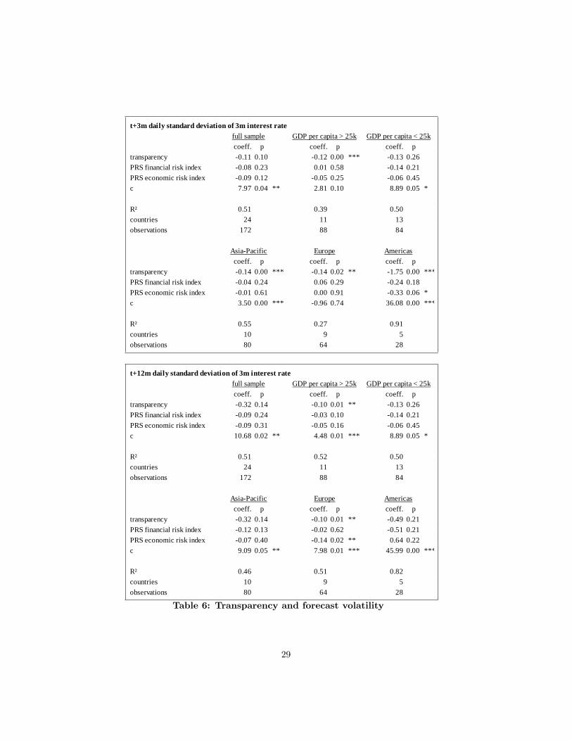
Results for the entire sample suggest that transparency does not have asignificant impact on the standard deviation of interest rates for the t to t + 3period. However, all but one of the subsamples shows a significant impact.The size of the estimated effect is similar across all subsamples, except for theAmericas subsample, where the estimate is probably largely driven by the highvolatility of Argentina’s interest rates in a small sample. The estimates for theentire sample and the subsamples are also economically meaningful consideringthe average standard deviation of 0.5%-point reported in Table 2.
The evidence for the impact of transparency on the standard deviation ofinterest rates for the t to t+12 period is weaker. Results are only significant forhigh income countries and Europe subsamples. There the reduction in volatilityis similar in scale to the results for the t to t+ 3 period.
Unlike the results for the forecast errors, removing Argentina from the sam-ple has a substantial impact on the significance of the results.
t+3m daily standard deviation of 3m interest rate
coeff. p coeff. ptransparency 0.14 0.00 *** 0.16 0.00 ***PRS financial risk index 0.00 0.96 0.02 0.68PRS economic risk index 0.03 0.12 0.01 0.70c 2.71 0.00 *** 2.77 0.02 **
R² 0.37 0.29countries 23 12observations 168 80
t+12m daily standard deviation of 3m interest rate
coeff. p coeff. ptransparency 0.11 0.03 ** 0.11 0.28PRS financial risk index 0.07 0.14 0.08 0.38PRS economic risk index 0.10 0.17 0.11 0.37c 8.20 0.03 ** 8.66 0.04 **
R² 0.46 0.40countries 23 12observations 168 80
full sample GDP per capita < 25k
full sample GDP per capita < 25k
Table 7: Transparency and interest rate volatility,without Argentina
30
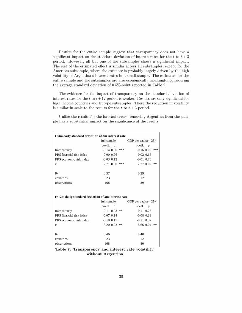
Without Argentina, the full sample results are clearly significant for both thethree month and twelve month volatility measures. The three month volatilitymeasure for the low income countries is also highly significant.
As noted in the section on data, the time frames of the volatility measureare, in practice, somewhat different than that of the forecast errors, helping toexplain why the coeffi cients for three and twelve month volatility are closer to-gether than for the forecast errors. Nevertheless, the overall pattern runs parallelto that of the forecast errors: transparency reduces volatility and the reductionis greater at a shorter time frame and fades over a longer time frame. The the-oretical prediction, presented in the Section 2, that transparency, predictabilityand market stability are closely related is therefore supported by these results.Likewise, the purported benefit of transparency at fostering financial marketstability is supported by the evidence presented above.
6 Conclusion
Central bankers have sought to improve the predictability of monetary policyas a way to reduce interest rate volatility and thereby enhance economic sta-bility. While some theoretical and experimental papers, including contributionsby the author, suggest that central bank transparency might actually harm pre-dictability by hampering the use of private information, most empirical work hasfound these concerns to be unwarranted. Such research, however, has generallyonly compared average predictability before and after some watershed trans-parency reform and done so only for a limited number of advances economies.My approach has a broader scope because I examine the relationship betweenthe Dincer and Eichengreen transparency index and predictability for twenty-four countries with varying levels of income. Furthermore, I use professionalforecasts, which have seen limited use in multi-country predictability analysis.Finally, I also examine interest rate volatility, to see if predictability and trans-parency do indeed go hand-in-hand, something which is not extensively done inthe literature.
The results provide improved empirical evidence that supports the generalfinding that transparency is beneficial and does so for a broad set of coun-tries. Forecast errors decline significantly for the three month ahead forecasts,although not at the horizon of one year. My evidence also suggests that thevolatility of interest rates do indeed track predictability. Greater transparencyis accompanied by a significant decline in interest rate volatility.
31
References
Bauer, A., Eisenbeis, R., Waggoner, D. and Zha, T.: 2006, Transparency, ex-pectations and forecasts. Federal Reserve Bank of Atlanta Working Paper2006-3.
Berger, H., Ehrmann, M. and Fratzscher, M.: 2006, Forecasting ECB monetarypolicy: Accuracy is (still) a matter of geography? ECB Working PaperNo. 578.
Bernanke, B.: 2004, Central bank talk and monetary policy. Speech, 7 October.
Blinder, A., Ehrmann, M., Fratzscher, M., de Haan, J. and Jansen, D.-J.: 2008,Central bank communication and monetary policy: A survey of theory andevidence. CEPS Working Paper.
Campbell, J. Y. and Shiller, R. J.: 1991, Yield spreads and interest rate move-ments: A bird’s eye view, The Review of Economic Studies 58(3), 495—514.
Carlson, J., Craig, B., Higgins, P. and Melick, W.: 2006, FOMC communicationsand the predictability of near-term policy decisions. Federal Reserve ofCleveland Review.
Cecchetti, S. G. and Hakkio, C.: 2009, Inflation targeting and private sectorforecasts. NBER Working Paper No. 15424.
Cochrane, J. H. and Piazzesi, M.: 2005, Bond risk premia, American EconomicReview 95(1), 138—160.
Coppel, J. and Connolly, E.: 2003, What do financial market data tell us aboutmonetary policy transparency? Reserve Bank of Australia Working Paper.
Crowe, C.: 2006, Testing the transparency benefits of : Evidence from privatesector forecasts. IMF Working Paper 06/289.
Crowe, C. and Meade, E. E.: 2008, Central bank independence and trans-parency: Evolution and effectiveness. IMF Working Paper 08/119.
Dale, S., Orphanides, A. and Osterholm, P.: 2008, Imperfect central bank com-munication - information vs. distraction. IMF Working Paper 08/60.
Demertzis, M. and Hoeberichts, M.: 2007, The costs of increasing transparency,Open Economies Review 18, 263—280.
Dincer, N. and Eichengreen, B.: 2007, Central bank transparency: Where, whyand with what effects? NBER Working Paper No. 13003.
Ehrmann, M., Eijffi nger, S. and Fratzscher, M.: 2010, The role of central banktransparency for guiding private sector forecasts. ECB Working Paper No.1146.
32
Ehrmann, M. and Fratzscher, M.: 2007, Social value of public information:Testing the limits of transparency. ECB Working Paper No. 821.
Eijffi nger, S. and Geraats, P.: 2006, How transparent are central banks?, Euro-pean Journal of Political Economy 22, 1—21.
Fama, E. F. and Bliss, R. R.: 1987, The information in long-maturity forwardrates, The American Economic Review 77(4), 680—692.
Hayford, M. and Malliaris, A.: 2007, Transparent monetary policy. LoyolaUniversity Chicago Working Paper.
Hayo, B. and Neuenkirch, M.: 2009, Does FOMC communication help predict-ing federal funds target rate changes? MAGKS Joint Discussion PaperSeries in Economics, No. 25-2009.
Holmsen, A., Qvigstad, J. F., Øistein Røisland and Solberg-Johansen, K.: 2008,Communicating monetary policy intentions: The case of Norges Bank.Norges Bank Working Paper 2008-20.
Jansen, D.-J. and de Haan, J.: 2009, Has ECB communication been helpful inpredicting interest rate decisions? an evaluation of the early years of theeconomic and monetary union, Applied Economics 41(16), 1995—2003.
Johnson, D.: 2002, The effect of inflation targeting on the behavior of expectedinflation, Journal of Monetary Economics 49, 1521—1538.
Kool, C., Middeldorp, M. and Rosenkranz, S.: 2011, Central bank transparencyand the crowding out of information in the financial markets, Journal ofMoney, Credit and Banking . Forthcoming.
Kwan, S.: 2007, On forecasting future monetary policy: Has forward-lookinglanguage mattered? Federal Reserve Bank of San Francisco EconomicLetter 2007-15.
Lange, J., Sack, B. and Whitesell, W.: 2003, Anticipations of monetary policy infinancial markets, Journal of Money, Credit and Banking 35(6), 889—909.
Lildholdt, P. and Wetherilt, A. V.: 2004, Anticipation of monetary policy inUK financial markets. Bank of England Working Paper 241.
Linder, A. and Santiso, C.: 2002, Assessing the predictive power of country riskratings and governance indicators. Paul H. Nitze School of Advanced Inter-national Studies of Johns Hopkins University Working Paper WP/02/02.
Mariscal, I. B.-F. and Howells, P.: 2006a, Monetary policy transparency in theUK: The impact of independence and inflation targeting. University ofWest England, Bristol Working Paper.
33
Mariscal, I. B.-F. and Howells, P.: 2006b, Monetary policy transparency, lessonsfrom Germany and the Eurozone. University of West England, BristolWorking Paper.
Middeldorp, M.: 2011, FOMC communication policy and the accuracy of Fedfunds futures. Federal Reserve Bank of New York Staff Report 491.
Middeldorp, M. and Rosenkranz, S.: 2011, Central bank communication andthe crowding out of private information in an experimental asset market.Federal Reserve Bank of New York Staff Report 487.
Mizen, P.: 2009, What can we learn from central bankers’words? some non-parametric tests for the ECB, Economic Letters 103, 29—32.
Morris, S. and Shin, H. S.: 2002, Social value of public information, The Amer-ican Economic Review 92(5), 1521—1534.
Murdzhev, A. and Tomljanovich, M.: 2006, What is the color of AlanGreenspan’s tie? how central bank policy announcements have changedfinancial markets, Eastern Economic Journal 32(4).
Piazzesi, M. and Swanson, E.: 2008, Futures prices as risk-adjusted forecasts ofmonetary policy, Journal of Monetary Economics 55, 677—691.
Rafferty, M. and Tomljanovich, M.: 2002, Central bank transparency and mar-ket effi ciency: An econometric analysis, Journal of Economics and Finance26(2), 150—161.
Sack, B.: 2004, Extracting the expected path of monetary policy from futuresrates, The Journal of Futures Markets 24(8), 733—754.
Stambaugh, R. F.: 1988, The information in forward rates, Journal of FinancialEconomics 21, 41—70.
Sturm, J.-E. and de Haan, J.: 2009, Does central bank communication reallylead to better forecasts of policy decisions? new evidenced based on aTaylor rule model for the ECB. KOF Working Paper 2009 No. 236.
Svensson, L. E.: 2006, Social value of public information: Morris and shin (2002)is actually pro transparency, not con, The American Economic Review96(1), 448—452.
Swanson, E.: 2006, Have increases in Federal Reserve transparency improvedprivate sector interest rate forecasts, Journal of Money, Credit and Banking38, 792—819.
Tomljanovich, M.: 2004, Does central bank transparency impact financial mar-kets? a cross country econometric analysis, Southern Economic Journal.
van der Cruijsen, C. and Eijffi nger, S.: 2007, The economic impact of centralbank transparency: A survey. CEPR Working Paper No. 6070.
34
7 APPENDIX —Transparency Checklist
Text copied directly from Appendix of Dincer and Eichengreen (2007)
This appendix describes the construction of the transparency index. Theindex is the sum
of the scores for answers to the fifteen questions below (min = 0, max = 15).
1. Political Transparency
Political transparency refers to openness about policy objectives. This com-prises a formal statement of objectives, including an explicit prioritization incase of multiple goals, a quantification of the primary objective(s), and explicitinstitutional arrangements.
(a) Is there a formal statement of the objective(s) of monetary policy, withan explicit prioritization in case of multiple objectives?
No formal objective(s) = 0.
Multiple objectives without prioritization = 1/2.
One primary objective, or multiple objectives with explicit priority = 1.
(b) Is there a quantification of the primary objective(s)?
No = 0.
Yes = 1.
(c) Are there explicit contacts or other similar institutional arrangementsbetween the monetary authorities and the government?
No central bank contracts or other institutional arrangements = 0.
Central bank without explicit instrument independence or contract = 1/2.
Central bank with explicit instrument independence or central bank contractalthough possibly subject to an explicit override procedure = 1.
2. Economic Transparency
Economic transparency focuses on the economic information that is usedfor monetary policy. This includes economic data, the model of the economythat the central bank employs to construct forecasts or evaluate the impact ofits decisions, and the internal forecasts (model based or judgmental) that thecentral bank relies on.
35
(a) Is the basic economic data relevant for the conduct of monetary policypublicly available? (The focus is on the following five variables: money supply,inflation, GDP, unemployment rate and capacity utilization.)
Quarterly time series for at most two out of the five variables = 0.
Quarterly time series for three or four out of the five variables = 1/2.
Quarterly time series for all five variables = 1.
(b) Does the central bank disclose the macroeconomic model(s) it uses forpolicy analysis?
No = 0.
Yes = 1.
(c) Does the central bank regularly publish its own macroeconomic forecasts?
No numerical central bank forecasts for inflation and output = 0.
Numerical central bank forecasts for inflation and/or output published atless than quarterly frequency = 1/2.
Quarterly numerical central bank forecasts for inflation and output for themedium term (one to two years ahead), specifying the assumptions about thepolicy instrument (conditional or unconditional forecasts) = 1.
3. Procedural Transparency
Procedural transparency is about the way monetary policy decisions aretaken.
(a) Does the central bank provide an explicit policy rule or strategy thatdescribes its monetary policy framework?
No = 0.
Yes = 1.
(b) Does the central bank give a comprehensive account of policy deliber-ations (or explanations in case of a single central banker) within a reasonableamount of time?
No or only after a substantial lag (more than eight weeks) = 0.
Yes, comprehensive minutes (although not necessarily verbatim or attributed)or explanations (in case of a single central banker), including a discussion ofbackward and forward-looking arguments = 1.
36
(c) Does the central bank disclose how each decision on the level of its mainoperating instrument or target was reached?
No voting records, or only after substantial lag (more than eight weeks) =0.
Non-attributed voting records = 1/2.
Individual voting records, or decision by single central banker = 1.
4. Policy Transparency
Policy transparency means prompt disclosure of policy decisions, togetherwith an explanation of the decision, and an explicit policy inclination or indi-cation of likely future policy actions.
(a) Are decisions about adjustments to the main operating instrument ortarget announced promptly?
No or only after the day of implementation = 0.
Yes, on the day of implementation = 1.
(b) Does the central bank provide an explanation when it announces policydecisions?
No = 0.
Yes, when policy decisions change, or only superficially = 1/2.
Yes, always and including forwarding-looking assessments = 1.
(c) Does the central bank disclose an explicit policy inclination after everypolicy meeting or an explicit indication of likely future policy actions (at leastquarterly)?
No = 0.
Yes = 1.
5. Operational Transparency
Operational transparency concerns the implementation of the central bank’spolicy actions. It involves a discussion of control errors in achieving operatingtargets and (unanticipated) macroeconomic disturbances that affect the trans-mission of monetary policy. Furthermore, the evaluation of the macroeconomicoutcomes of monetary policy in light of its objectives is included here as well.
(a) Does the central bank regularly evaluate to what extent its main policyoperating targets (if any) have been achieved?
37
No or not very often (at less than annual frequency) = 0.
Yes but without providing explanations for significant deviations = 1/2.
Yes, accounting for significant deviations from target (if any); or, (nearly)perfect control over main operating instrument/target = 1.
(b) Does the central bank regularly provide information on (unanticipated)macroeconomic disturbances that affect the policy transmission process?
No or not very often = 0.
Yes but only through short-term forecasts or analysis of current macroeco-nomic developments (at least quarterly) = 1/2.
Yes including a discussion of past forecast errors (at least annually) = 1.
(c) Does the central bank regularly provide an evaluation of the policy out-come in light of its macroeconomic objectives?
No or not very often (at less than annual frequency) = 0.
Yes but superficially = 1/2.
Yes, with an explicit account of the contribution of monetary policy in meet-ing the objectives = 1.
38