Embed Size (px)
Citation preview

CENTRAL BANK OF NIGERIA
ISSN 1957-2968
Test of the Fisher Effect in NigeriaTule, M. K., U. M. Okpanachi, E. T. Adamgbe and
S. E. Smith
Effect of Monetary Policy on Agricultural Sector
in NigeriaUdeaja, E. A. and E. A. Udoh
An Autoregressive Distributed Lag (ARDL) Approach
to the Oil Consumption and Growth Nexus:
Nigerian EvidenceInuwa N., H. M. Usman and A. M. Saidu
Economic and Financial Review
Economic and Financial ReviewVolume 52, Number 2
June 2014
Volume 52, Number 2
June 2014 O K FAN N B ILA GER RTN IAEC

Central Bank of Nigeria
Economic and Financial ReviewVolume 52, Number 2, June 2014Aims and ScopeThe Economic and Financial Review is published four times a year in March, June, September and December by the Research Department of the Central Bank of Nigeria. The Review contains articles on research undertaken at the Bank, in particular, and Nigeria, in general, mainly on policy issues both at the macroeconomic and sectoral levels in the hope that the research would improve and enhance policy choices. Its main thrust is to promote studies and disseminate research findings, which could facilitate achievement of these objectives. Comments on or objective critiques of published articles are also featured in the review.
CorrespondenceCorrespondence regarding the Economic and Financial Review and published articles should be addressed to:
Director of Research/Editor-in-ChiefCBN Economic and Financial ReviewCentral Bank of Nigeria33 Tafawa Balewa WayCentral Business DistrictP. M. B. 0187 GarkiAbujaNigeria
Email: [email protected]: www.cbn.gov.ng
SubscriptionSubscription to the Central Bank of Nigeria Economic and Financial Review is available without charge to institutions, corporations, embassies, and development agencies. Individuals can send written request for any particular edition of interest, also without charge. Articles may be reprinted, reproduced, published, abstracted, and distributed in their entirety on condition that the author and the source—Central Bank of Nigeria Economic and Financial Review—are duly credited.
DisclaimerAny opinions expressed in the Economic and Financial Review are those of the individual authors and should not be interpreted to represent the views or policies of the Central Bank of Nigeria, its Board of Directors or its Management.
Notes to ContributorsInformation on manuscript submission is provided on the last and inside back cover of the Review.
Editorial Committee
Editor-in-Chief
Charles N. O. Mordi
Managing EditorBanji S. Adebusuyi
Editor
Associate EditorsAdeniyi O. Adenuga
© Copyright 2014
Central Bank of
Nigeria
ISSN 1957-2968

Contents
Test of the Fisher Effect in Nigeria
Tule M. K., U. M. Okpanachi, E. T. Adamgbe and S. E. Smith ...........................1
Effect of Monetary Policy on Agricultural Sector in Nigeria
Udeaja, E. A. and Elijah A. Udoh .............................................................................. 33
An Autoregressive Distributed Lag (ARDL) Approach to the Oil
Consumption and Growth Nexus: Nigerian Evidence
Inuwa, N., H. M. Usman and A. M. Saidu .................................................................. 75
Central Bank of Nigeria Economic and Financial ReviewVolume 52, No. 2, June 2014


A Test of the Fisher Effect in NigeriaTule, M. K., U. M. Okpanachi, E. T. Adamgbe and S. E. Smith
Abstract
Keywords: Fisher Effect, State space model, co-integration
JEL Codes: E31, E43, C32
The “Fisher Effect” has stimulated enormous research interest, especially in monetary policy.
Expectedly, empirical evidence has varied greatly – from absence of effect to strong effect.
This has kept the debate alive, with the benefit of fresh policy-relevant insights and clues
especially in developing countries where the literature on the subject is fast growing. This
paper contributes to the debate by using the state space model to investigate the dynamic
relationship between real interest rate and inflation in Nigeria. The paper reveals varying
degrees of effect across interest rate and time horizons.
Tule, M. K., U. M. Okpanachi, S. E. Smith and E. T. Adamgbe are staff of the Monetary Policy and Research Departments, Central Bank of Nigeria. The views expressed in this paper are those of the author and do not necessarily reflect the opinions of the Central Bank of Nigeria.
I. Introduction
he conclusion of Fisher (1930) concerning the relationship between changes
in short-term interest rates and expected inflation has continued to elicit Tconsiderable discussion and research in both academic and policy circles
globally. Several empirical studies have been carried out across industrialised and
non-industrialised countries on the subject matter. Fisher had posited that nominal
interest rate adjusted one-to-one to changes in expected inflation. If this were
indeed the case, then, movements in rates should contain vital information about
the direction and level of prices in the future. However, empirical evidence on the
subject matter has varied from one country to another and across periods.
The relationship between inflation expectation and nominal interest rate is crucial
for monetary policy. Continuous examination of this relationship is warranted by
the inconclusive nature of available evidence and the likelihood that such a
relationship, even if established, may not be permanent. Fisher effect studies have
seemingly gained additional impetus and momentum as inflation targeting
Central Bank of Nigeria Economic and Financial Review Volume 52 No. 2 June 2014 1
became popular. The reason is simple – it relies on the use of short-term rates, often
overnight rate as an intermediate target. The vastness of the literature on
industrialised countries in particular, is therefore, not surprising. Interest rate plays a
pivotal role in the economy. The viability of Fisher's hypothesis holds overarching
implications for monetary policy and, therefore, significant for central banks as
well.
In the developing world, the literature on the Fisher's effect is growing. Some studies
have pooled developing countries along with advanced countries in multi-
country analysis, with most suggesting that the Fisher Effect is either absent or not
very strong in these countries (Berument and Jelassi, 2002). Some others have
provided contrary indications. Maghyereh and Zoubi (2006), for example,
reported a strong Fisher Effect in Turkey, Brazil, Argentina, Mexico and Malaysia. As
such, any generalisation about the Fisher Effect in a developing country could
easily be misleading. Country-specific studies will continue to be relevant in
providing contextual analysis and informed conclusions.
The Central Bank of Nigeria (CBN) like others in developing countries would find
studies of this nature useful in enriching evidence needed to support the conduct
of monetary policy generally, and particularly in evaluating policy instruments.
There are currently only a few studies conducted using Nigerian data to verify this
very important proposition.
In Nigeria, the Central Bank of Nigeria (CBN) is the sole monetary authority and its
policy stance has continued to evolve. In 2006, the Bank introduced the Monetary
Policy Rate (MPR) and a standing deposit/lending facility with a corridor around
1the MPR as part of its monetary policy implementation framework . Prior to this
time, the Bank used the Minimum Rediscount Rate (MRR) to influence interest rates
and lending decisions of banks. The MRR was found to be ineffective as it neither
2 Central Bank of Nigeria Economic and Financial Review June 2014
1Both the lending and deposit facilities are always available to banks and have helped them to manage their liquidity positions better than previously. They have also reduced the desperation that hitherto characterised activities at the interbank in times of liquidity scarcity thereby helping to reduce volatility in rates at the interbank.

anchored inflation expectations nor short-term interest rates. In fact, for a long time
the MRR was unchanged at 14.0 per cent, serving simply as the Bank's rediscount
rate.
The introduction of the MPR and the standing deposit/lending facility, following the
refinement of the framework, proved to be useful as interbank rates started to
show some response to the adjustment decisions of the Bank's Monetary Policy
Committee (MPC) with regards to both policy rate and the corridor. Since 2006, the
MPR and corridor have been changed on many occasions in response to
2prevailing macroeconomic and market liquidity conditions . Both the
collateralised open buy back (OBB) and uncollateralised interbank call (IBR) have
mostly oscillated within the corridor. In addition, by manipulating the MPR the
Bank has been able to gain some influence on inflation expectations.
Nigeria's inflation history is mixed with episodes of high and low inflation. The
country's worst inflation experience was in the 1990s when inflation rose to above
60.0 per cent. The last ten (10) years have witnessed relatively moderate inflation of
less than 20.0 per cent. As monetary policy became more proactive following
recent refinements in strategy, inflation outcomes have tended to improve. In fact,
year-on-year inflation has not exceeded 15 per cent in the last 5 years. In 2013,
inflation was subdued within single digit owing mainly to prolonged tight monetary
policy stance. Until the deregulation of the financial system in 1986, interest rates
were not market determined and were mostly at a low level applicable to both
domestic assets and liabilities of the banking system. The aftermath of the
deregulation resulted in an increase in lending rates, which rose in excess of 20.0
per cent on non-prime assets during most of the period up to 2013. Savings and
deposit rates have, however, remained relatively low, leaving wide spreads
between lending and savings rates.
Tule et. al,: A Test of the Fisher effect in Nigeria 3
2At inception, the MPR was set at 10.0 per cent with a symmetric corridor of 200 basis points above for the lending facility and below for the deposit facility. There have been occasions since then when the Bank implemented the asymmetric variant of the corridor. Currently, the MPR is 12.0 with 200 basis points symmetric corridor.

The objective of this paper is to investigate the dynamic relationship between
inflation and interest rates in Nigeria. The paper tested the Fisher Effect in Nigeria
focusing on the basic hypothesis that inflation and nominal interest rates exhibit a
proportional relationship.
This paper is unique in its contribution to the literature on Fisher's Effect in Nigeria on
the premise that it provides empirical evidence to support policy decisions
especially on the impending Inflation Targeting Framework (IT) of the Central Bank
by informing the choice of policy instruments. The questions this paper aims to
answer are: (i) Does the Fisher Effect Hold in Nigeria?, If yes; how strong is the
effect? and (ii) Is there any inter-temporal variations in the Effect or is the Fisher's
Effect time-invariant?
This paper is structured into 6 sections. Following this introduction, section 2 reviews
the theoretical and empirical literature while section 3 presents the modelling
technique and the empirical methodology. The data and modeling of the
variables are presented in Section 4. Section 5 is a presentation and analysis of the
results while section 6 concludes with some policy recommendations.
II. Literature Review
II.1 Theoretical Review
3The idea that gave birth to the Fisher' Effect was initially expressed in Fisher (1896) .
His hypothesis about inflation and interest rates which became known as the
Fisher's Effect was, however, formally and fully developed much latter in Fisher
4(1930) . Based on the findings of the study in the U.S and U.K, Fisher came to the
conclusion that long-run, nominal interest rate is given by the sum of expected
inflation and expected real interest rate. Simply, the Fisher’s equation otherwise
referred to as the Fisher’s parity may be symbolically stated as:
* * R = r + ð
4. Central Bank of Nigeria Economic and Financial Review June 2014
3Irving Fisher's work, “Appreciation and Interest” published in 1896 provided the first clue about what was later called the Fisher's Effect.4“Theory of Interest”

where: * * R is nominal rate of interest, r is expected real interest rate and ð is expected
5 *inflation . Based on the premise that expected real interest rate (r ) is constant,
nominal interest rate should vary point-for-point with inflation.
’ * ’ * *F (r ) = 0, while F (ð ) = 1; therefore, R varies with ð point-for-point.
If inflation rises by x per cent as a result of monetary expansion, the nominal interest
rate also adjusts upwards by the same magnitude. The Fisher’s proposition of one-
to-one adjustment between inflation and nominal interest rate was inferred from
his estimates of the relationship between interest rates and inflation in Britain over
the period 1890 to 1924 and in the U.S., 1890 to 1927. Fisher used the distributed lag
structure with arithmetically declining lags to model inflation expectation. Some
studies have used either the same or a variant of the original Fisher’s approach in 6modeling inflation expectation (Sargent 1969 and Gibson 1972) .
Following this exposition by Fisher, very many empirical investigations have been
conducted on the same countries studied by Fisher and on several others.
Analytical methods, results and conclusions have varied in many respects. If
Fisher’s Effects holds, then real interest rates must be independent of monetary
policy working through expected inflation and long-run nominal interest rates.
However, there have been some other propositions that appear to negate the
Fishers’ consequence. For example, whilst not denying the existence of a positive
relationship between inflation and nominal interest rates, some scholars have
argued that the proposition of one-to-one could not possibly hold since inflation
reduces money balances (Mundel, 1963 and Tobin, 1965).
In a related sense, it is argued that the Fisher’s relationship breaks down in the face
of prolonged Quantitative Easing (QE) due to what is referred to as ‘policy duration
effect’.
Tule et. al,: A Test of the Fisher effect in Nigeria 5
5 * *This relation is stated in various forms such as r = R - ð 6Following the development of rational expectations by Muth (1961) and efficient markets by Fama (1975), the approach to handling the unobservable inflation expectations shifted a bit. Fama (1975) and Levi and Makin (1979-Not listed (NL) on the reference list) were among the earliest to incorporate the new thinking in the analysis of the Fisher's Effect.

(Okina and Shirasuka, 2004). Policy duration effect arises from expectations of the
duration of monetary easing into the future. They further argued that prolonged
quantitative easing leads to the formation of stable market expectations about
short-term interest rates which cause long-term rate to fall, flattening the yield
curve. Inflation expectations could however, remain unchanged because the
market is rather concerned with how long the QE would last than the current
surplus liquidity. As nominal interest rate falls leaving inflation expectations
unchanged, the real economy benefits making monetary policy able to impact
on long-run growth.
Soderlind (2001) finds that a very active monetary policy or stricter inflation
targeting reduces the strength of the relationship between nominal rates and
inflation. Mitchell-Innes (2006) confirms this for South Africa, noting that in the long-
run, adjustment of interest rates to inflation is less than unity which he attributed to
the success of inflation targeting in meeting inflation expectations within the target
range.
II.2 Empirical Literature
II.2.1 Evidence from Advanced Countries
Fisher’s hypothesis received tremendous attention in industrialised countries owing
to the substantial studies that showed significant relationship between inflation
and nominal interest rates. However, evidence on the stability of the one-to-one
relationship between the two, remains quite conflicting. The estimated slope
coefficients of nominal interest rates on various measures of expected inflation
have been shown to be substantially lower than ‘1’, the theorised value (Fama and
Gibson, 1984; Huizinga and Mishkin 1986). These studies have nonetheless shown
7that real interest rates are negatively associated with expected inflation .
The observed less than proportional reaction of interest rates to changes in
expected inflation as observed in most empirical studies has commonly been
6 Central Bank of Nigeria Economic and Financial Review June 2014
7A few other studies, for example Darby (1975), have reported results suggesting that the adjustment of interest rate to expected inflation could be higher than 1.

referred to in the literature as the Fisher Effect Puzzle (Mishkin and Simon, 1995).
Test of the Fisher hypothesis in advanced economies although inconclusive,
apparently reveals some time-varying effects and country-specific outcomes. The
evidence portrays not very distinctive but an emerging differential along the time
periods and tools of analysis. Studies such as Fama (1979), Nelson and Schwert
(1977), Mishkin (1984, 1988) and Fama and Gibbsons (1984) have indicated a
strong post-war Fisher effect in the U.S, UK and Canada up till 1979, but a reduced
effect post-1979. However, a correlation analysis by Mishkin and Simon (1995)
indicated a weak nominal interest rates and inflation nexus. Using the Johansen
co-integration technique, Hawtrey (1997) failed to find the Fisher effect for Austria
over the periods of 1969 to 1994 and 1969 to 1983. This finding corroborated Inder
and Silvapulle (1993) that used ECM for the period, 1965 to 1990.
Mishkin and Simon (1995) segmented their study sample into three, 1962 to 1993,
1962 to 1979 and 1979 to 1993 and applied the Engle and Granger approach to
show that the Fisher Effect exist in the long-run and it was absent in the short-run.
However, Atkins and Sun (2003) used the discrete wavelet transformation
technique to investigate Fisher Effect for Canada. The study which covered the
period, 1959 to 2002, found support for the long-run Fisher Effect. The robustness of
this finding was, however, contested by several studies. In Olekalns (1996), using
Austrian data and applying ARCH and Maximum likelihood estimation techniques
from 1969 to 1993 there was little evidence of a long-run Fisher Effect. Also,
Choudhry (1997) applied the Engle and Granger estimation technique for the
period 1955 to 1994 with little evidence of a long-run Fisher Effect in Belgium; Atkins
and Serletis (2002) used the Pesaran et. al. (2001), estimation techniques for the
period 1880 to 1983 and found little support for a long-run Fisher effect in Norway,
Sweden, Italy, Canada, the United Kingdom, and the United States.
In a more recent study Ramadanoviæ (2011) used monthly data of long-term rates
to test for the Fisher hypothesis. The evidence did not support the presence of a
long-run equilibrium relationship between inflation and nominal interest rates in the
Tule et. al,: A Test of the Fisher effect in Nigeria 7

United Kingdom, Switzerland and Germany.
Panopoulou (2005) examined the Fisher effect using both short-term and long-
term interest rates in 14 OECD countries. Sufficient evidence was found to support
the existence of a long-run Fisher effect. However, application of a discrete
wavelet transformation (DWT) to the series as an alternative for the more
commonly used differencing approach by Atkins and Sun (2003) found evidence
of a Fisher effect for Canada and the United States, using data from 1959 to 2002.
Atkins and Coe (2002) used the ARDL Technique to investigate for the Fisher effect
in Canada. They used data from 1953 to 2000 and found evidence in support of the
Fisher Effect. Other studies that provided evidence in support of the Fisher Effect in
Canada include Dutt and Ghosh (1995), Crowder (1997) and Lardic and Mignon
(2003); while those that found no support in the same country include Ghazali and
Ramlee (2003) and Yuhn (1996).
II.2.2 Evidence from Emerging and Developing Countries
Mitchell-Innes (2006) examined the Fisher Effect under an inflation targeting
regime for South Africa using the 3-month bankers’ acceptance rate and the 10-
year government bond rate as substitutes for short- and long-term interest rates.
The data used in the study covered April 2000 to July 2005. The short-run Fisher
Effect was not empirically established, while long-term interest rates and expected
inflation were found to exhibit a long-run co-integrating relationship. Similarly for
South Africa, Wesso (2000) used the Johansen estimation technique to examine
whether a relationship exists for the period 1985 to1999 with little evidence of a
long-run Fisher Effect. Cooray (2002) examined Sri Lankan data for the presence of
Fisher Effect using the Johansen estimation technique. The data covered the
period, 1952 to 1998 but finds no evidence of the Fisher Effect. In Turkey, Aksoy and
Kutan (2002), using the GARCH estimation technique found no support in the
analysis for the long-run Fisher Effect.
From Latin America comes some strong evidence of the Fisher Effect. Carneriro et.
al., (2002) examined the Argentine economy for the Fisher Effect using the
8 Central Bank of Nigeria Economic and Financial Review June 2014

Johansen estimation technique using data from 1980 to 1997. The authors confirm
a long-run Fisher Effect. Earlier, Garcia (1993) and Phylaktis and Blake (1993) found
evidence of a long-run Fisher Effect in Brazil and Argentina. Jorgensen and Terra
(2003) also investigated the effect in Latin America using a four variable VAR
estimation technique. They found no evidence of a long-run relationship between
nominal interest rate and inflation for Brazil, Peru and Chile. Their results, however,
supported a long-run Fisher Effect in Mexico and Argentina. Studies by Asemota
and Bala (2013) and Obi et. al., (2009) on Nigeria using error correction and Kalman
filtration support the existence of a partial Fisher Effect for the period between 1961
and 2009.
III. Methodology
III.1 Data Sources and Research Method
Monthly data for Nigeria between 1970 and 2013 were used to model the
relationship between inflation and short-term interest rate. Inflation is the year-on-
year change in consumer prices (Inf), while various interest rates were considered
such as three-month Nigerian Government Treasury Bills rate (NTB91), three-month
deposit rate (dr3m); inter-bank and lending rates. Interest rate series were
compiled from various CBN publications while inflation numbers were obtained
from the National Bureau of Statistics (NBS) inflation reports.
From the literature, we note a variety of methods for evaluating the relationship
between inflation and interest rate or the Fisher Effect. Early attempts at verifying
the Fisher Effect relied mostly on OLS regression of interest rate on inflation. The
major challenge was how to measure the unobservable inflation expectation. In
addition, OLS estimation requires that the variables are stationary in their levels.
More often than not interest rate and inflation series lack this highly essential
property. With integrated variables, OLS estimates are generally unreliable.
Mishkin (1992) outlined the reasoning and implications of the variables (interest
rate and inflation) displaying stochastic trends. Using monthly US data, Mishkin
found that interest rate and inflation exhibit common trend which signaled strong
Tule et. al,: A Test of the Fisher effect in Nigeria 9

10 Central Bank of Nigeria Economic and Financial Review June 2014
correlation between them. This approach has subsequently dominated Fisher
8Effect studies in both developed and developing countries .
Co-integration between inflation and interest rate imply long-run equilibrium
between the two variables, which in a way indicates some Fisher Effect. However,
a slightly different argument is emanating, which seems to suggest that co-
integration between nominal interest rate and inflation should be more
appropriately seen as only a necessary condition for Fisher effect. The sufficient
condition is that nominal interest rate should embody an optimal inflation forecast
9(Miron, 1991) . This dimension calls for the application of other estimation
techniques that can more efficiently handle expectations as supplements to the
usual co-integration analysis.
Against the foregoing background, this paper employs a state space model
following Hamilton (1994) and others as well as a co-integration analysis, to
examine Nigerian data for the Fisher’s Effect. Unlike the fixed coefficients that co-
integration yields, the state space model provides time-varying parameters which
provide some insights about the inter-temporal stability or otherwise of parameters
(Hamilton, 1994).
III.2. Model Specification
III.2.1 The State Space Model
The state space framework (SSF), given its time-varying properties, provides an
informative approach to analysis of the inflation-nominal interest rate relationship.
In particular, unlike forecast based methods applied in Million (2004), the SSF is
preferred for its ability to estimate unobserved components such as inflation
expectations. In addition, when inflation expectation time series generated for
such forecast based expectations and other approaches are not available, the
SSF becomes a useful tool in the study of the nominal interest rate-inflation
8See examples: Mishkin and Simon (1995), Crowder (1997), Dutt and Ghosh (1995), Lee et. al., (1998) Cameiro et. al., (2002), and Granville and Mallick (2004).9For a detailed and more comprehensive presentation of this idea, see Johnson (2005).

Tule et. al,: A Test of the Fisher effect in Nigeria 11
relationship. Essentially, it uses the Kalman filter estimation to uncover the time
varying effect of inflation dynamics on the nominal interest rate. The general
specification of the state space model consists of a state (transition) and
measurement or signal (observation) equation. The state equation governs the
dynamics of the unobserved or state variables, while the measurement equation
relates the observed variable to the unobserved variable. A state space model
can be represented as follows:
(Signal equation)
(State equation)
In the signal or measurement equation, y represents a vector of measured t
variables of n by 1 dimension; gives the state vector of unobserved variables of m t
by 1 dimension; Z represents a matrix of parameters of n by m dimension and t
~ N (0, H ). In the state equation, is an m by m matrix, is an m by 1 vector, is an t t
arbitrary m by g matrix such that redefining the error term produces an SQS’
covariance matrix.
The Fisher relation (Fisher, 1930), postulates that the nominal rate of interest is the
sum of the ex-ante real interest rate and expected inflation suggesting that a
percentage change in the expected inflation will result in a change in the nominal
interest rate. Algebraically, this relation is expressed as:
(1)
In equation (1), is the nominal interest rate, is the ex-ante real rate, while
denotes the inflation expectation. In order to derive an expression for inflation
expectation, we consider the inflation forecast error , as the difference between
actual and expected inflation which we can express in the form:
(2)
From equation 2, we can re-arrange to obtain an expression for inflation
expectation as:
(3)
Under the assumption of rational expectation, the forecast error is assumed to be
stationary such that substituting for in equation (1) produces equation (4).
b
e a tT Rt t
?
()0,t t t t t ty c Z N tHbee=++ ~
() ~ 0,t N tQm 1t t t t t tT a Rbb m-=++
e et t ti r p=+
ti e
tr etp
tm
et t tmpp=-
et t tppm=+
etp

(4)
Thus, from equation 4, the ex post real rate, , is given as the addition of the ex-
ante real rate and the inflation forecast error. In the literature, an examination of
the Fisher effect involves fitting the nominal interest rate on the realised or actual
inflation. We form this equation by simply rearranging and parameterising
equation (4), thus:
(5)
To evaluate the Fisher effect, if the coefficient there exists a full Fisher effect, but
if it suggests a partial Fisher effect. However, equation (5) which is constant
parameterisation can be put in a state space form in order to capture the
changing role of monetary policy on the existence or otherwise of the Fisher effect,
i.e. to evaluate the time varying dimension of the Fisher effect. Thus, the state
space form of equation (5) is given by equation 6.
Equation (6a) represents the measurement equation, while equation (6b) and (6c)
are the state or transition equations for the time-varying intercept term and varying
effect of inflation on the real interest rate. The measurement equation relates real
interest rate and the unobserved state variable ( ) with the regression coefficient
at the beginning of the series, while the transition equation shows changing path of
the state variable and measures the association between the real interest rate and
inflation over time. The observation error and state error are assumed to be
white noise.
The first state series is a time-varying intercept ( ), that is, the values of the level at
the beginning of the series, whereas the second state series is a time-varying
measure of inflation persistence, that is, is the slope parameter.
To model inflation expectation, we similarly apply a state space model in equation
(7):
i-pt t
b=1 t
b<1 t
bt
m ht t
a
12 Central Bank of Nigeria Economic and Financial Review June 2014
et t t ti rp m-=+
et t t t tir bpm=++
et t t t ti r abptm-=++ (6a)
1t t t tFaau-=+ (6b)
1t tHb tbth-= + (6c)

As in the case of equation (6), the observation error is and the state errors and
are assumed to be white noise, while C is the drift parameter. t
This enables us using the Kalman filter to examine the time varying path of the state
( ) using observed data. In addition, it can help in establishing whether real interest
rate and inflation have common factors. The Kalman filter is a recursive algorithm
for carrying out computations in a state space model. Kalman Smoothing
produces a more precise estimate of the state vector or slope coefficient. The
unknown variance parameters ( and ) are estimated by the maximum
likelihood estimation via the Kalman filter prediction error decomposition initialised
with the exact initial Kalman filter.
IV. Modeling of Variables
IV.1 Data Patterns and Statistics
Three of the earlier identified series (inflation, NTB rate and 3-month deposit rate)
are shown graphically over the period, 1970 to 2013, on figures 1 and 2. Both charts
show some co-movement – though insufficient to conclude on the exact nature of
the relationship. Between 1970 and around the middle of the 1980s, interest rates
appear quite stable, almost flat but started showing minimal movements
thereafter. Inflation, on the other hand, rose and fell intermittently across the
sample period.
m e Vt t
bt
2 2s sm h
Tule et. al,: A Test of the Fisher effect in Nigeria 13
1t t t t tCp bpm-=++
1t t t tC F C e-=+
1t t t tZbbV-=+
(7a)
(7b)
(7c)

Figure 3 provides further insights about the nature and strength of the relationship
between inflation and interest rate. By connecting correlation coefficients
between interest rate and inflation at lags (1 – 25) we find a weak positive
correlation rising through from about 0.28 to 0.47 around lag 22, after which it starts
to diminish. This is not very suggestive of the strong relationship implied by the Fisher
hypothesis.
14 Central Bank of Nigeria Economic and Financial Review June 2014
Figure 1: NTB (91-day) rate and inflation (%)
1 0 0
8 0
6 0
4 0
2 0
0
- 2 01 9 7 0 1 9 7 5 1 9 8 0 1 9 8 5 1 9 9 0 1 9 9 5 2 0 0 0 2 0 0 5 2 0 1 0
N T B 9 1 I N F
Figure 2: 3-month deposit rate and inflation (%)
1 0 0
8 0
6 0
4 0
2 0
0
- 2 01 9 7 0 1 9 7 5 1 9 8 0 1 9 8 5 1 9 9 0 1 9 9 5 2 0 0 0 2 0 0 5 2 0 1 0
N T B 9 1 I N F

Sample statistics vary across periods, but more substantially for inflation (Table 1).
For example, while inflation averaged 19.69, 23.43, 17.95 and 10.8 for full, 1974 to
1993, 1994 to 2013 and 2007 to 2013 periods, respectively, NTB rate averaged 9.8,
9.16, 11.62 and 8.02 over the same periods. Expectedly, standard deviations are
higher for inflation and over the four sample periods, inflation standard deviations
are 17.9, 18.3, 17.98 and 3.02 compared with NBT's 5.65, 6.16, 4.67 and 3.77.
Table 1: Sample Statistics: Full and Sub-Periods
Tule et. al,: A Test of the Fisher effect in Nigeria 15
Figure 3: Correlations between NTB (91-day) rate and inflation (%)
Full sample correlation: interest rate and inflation
0.45
0.4
0.35
0.3
0.25
0.2
0.15
0.1
0.05
0
C
o
r
r
.
Inflation Lags
1 2 3 4 5 6 7 8 9 10 11 12 13 14 15 16 17 18 19 20 21 22 23 24 25
Full Sample
(1970-2013)
1974-1993 1994-2013 2007-2013
NTB91 3MDR
Inf
NTB91
3MDR
Inf NTB91
3MDR
Inf NTB91
3MDR
Inf
Mean 9.80 9.83
19.69
9.16
9.65
23.43
11.62
11.39
17.95
8.02
9.18
10.80
Maximum 28.00 27.00
89.57
28.00
27.00
67.60
24.50
23.60
89.57
15.00
14.65
15.59
Minimum 1.04 2.00
-4.98
2.50
2.00
-4.98
1.04
4.13
-2.49
1.04
4.13
4.12
Std. Dev.5.65 5.20 17.90 6.61 6.10 18.31
4.67 3.30 17.98 3.77 2.81 3.02

IV.2 Stationarity
Economic analysis using time series has continued to evolve with better
understanding of some of covert properties of the series. In one such refinement,
Sims (1980) showed that OLS regression of series that are integrated produces
spurious results. Following this realisation it is standard practice to check series for
stationary. The result of such an evaluation typically determines the choice of
modeling technique to be applied. Figure 4 show the series in levels and first
differences.
Figure 4 show inflation, NTB rates and deposit rate in levels and first differences side-
by-side. The differenced series show better convergence compared to the levels
that appear to drift. This is an early indication of the presence of unit root in the
series at their levels. After subjecting the series to two standard unit root tests (ADF
and Phillips-Peron), we found that they were all integrated of order 1 (Appendix 1).
This finding means that OLS modeling of the data will be inappropriate.
16 Central Bank of Nigeria Economic and Financial Review June 2014
Jarque 39.82 22.84
299.91 57.92
26.03
25.81 1.35
3.15
472.54 2.34
4.10
6.15
Prob. 0.00 0.00
0.00
0.00
0.00
0.00
0.51
0.21
0.00
0.31
0.13
0.05
Obs. 525 526
525
240
240
240
237
237
237
81
81
81
Figure 4: Series in levels and first differences
100
80
60
40
20
0
-201970 1975 1980 1985 1990 1995 2000 2005 2010
INF
30
20
10
0
-10
-201970 1975 1980 1985 1990 1995 2000 2005 2010
D (INF)

V. Presentation and Analysis of Results
V.1 Co-integration
Following from the stationary results presented in the previous section, the paper
proceeded to explore co-integration between inflation and interest rate – which
can be a basis for some preliminary inferences about Fisher effect. However, using
both the Engle and Granger and Phillips-Ouliaris techniques, the hypothesis of no
co-integration between short-term interest rates (proxied by the 91-day NTB rate
and 3-month deposit rate) and inflation was not rejected (see Appendices).
Absence of co-integration means that there is no long-run equilibrium relationship
10between the variables and, possibly, no Fisher Effect present . The finding of no co-
integration in the full sample (1970-2013) does not rule out the possibility of Fisher
effect occurring in sub-periods. To investigate this, the paper employs a suitable
technique – The state space model.
Tule et. al,: A Test of the Fisher effect in Nigeria 17
30
25
20
15
10
5
01970 1975 1980 1985 1990 1995 2000 2005 2010
NTB91
8
4
0
-4
-8
-12
-161970 1975 1980 1985 1990 1995 2000 2005 2010
D(NTB91)
30
25
20
15
10
5
01970 1975 1980 1985 1990 1995 2000 2005 2010
3MDR8
4
0
-4
-8
-121970 1975 1980 1985 1990 1995 2000 2005 2010
D(DR3M)
10Absence of co-integration generally diminishes the possibility of long-run Fisher Effect (Mishkin, 1992;
Johnson, 2005). The co-integration approach is limited in this wise. For studies using this approach, it
is practically the end the road.

V.2 State Space Model
In order to analyse the existence and extent of the Fishers’ Effect, the paper used
various interest rates - 90-day Treasury bill rate (TBR), maximum lending rate (MLR),
Prime lending rate (PLR), inter-bank call rate (IBCR) and 3-month deposit rate
(3MDR). This should help determine which interest rate is subject to the Fisher Effect.
Sequel to the estimations, however, the IBCR, PLR and 3MDR showed no evidence
of the nominal interest rate-inflation nexus. For robustness and sensitivity
evaluation, three measures of inflation were included in the estimation, namely,
expected inflation based on its natural trend (generated using equation 7), the
actual inflation and a backward-looking inflation, a one-period lag of the actual
inflation. The estimates are presented in Tables 2-7.
18 Central Bank of Nigeria Economic and Financial Review June 2014
Figure 5: Estimates of Ex ante TBR and Time-varying Fisher Coefficients
-6
-4
-2
0
2
4
6
1975 1980 1985 1990 1995 2000 2005 2010
2
4
6
8
10
12
14
16
18
20
1975 1980 1985 1990 1995 2000 2005 2010
Smoothed ex ante TBR (Sv1) State Estimate Smoothed Time-varying Fisher Effect Coefficient (Sv2) State Estimate
SV1 + 2 RMSE SV2 + 2 RMSE
Figure 5 illustrates the ex-ante Treasury bill rate and the time-varying fisher
coefficients. The literature review demonstrated that the nominal interest rate is
the sum of expected inflation and the ex-ante real interest rate signifying that a
percentage change in the expected inflation will result in a change in the nominal
interest rate. A fairly obvious inverse co-movement exists between the level of the
TBR and inflation rate which is suggestive of the coefficients as common factors. A
higher inflation implies a reduced real interest rate, while a higher or lower
coefficient on inflation reflected a concomitant change in the real interest rate as
shown in Figure 6.

Tule et. al,: A Test of the Fisher effect in Nigeria 19
Figure 6: Real Interest-Inflation Relationship
rt Level
0
-25
-50
-751970 1975 1980 1985 1990 1995 2000 2005 2010
hinf Level75
50
25
01970 1975 1980 1985 1990 1995 2000 2005 2010
Method: Maximum likelihood (Marquardt)
Sample: 1970M03 2013M09
Included observations: 523
Convergence achieved after 1 iteration
Final State Root MSE z-Statistic Prob.
Ex-ante TB rate (SV1) 8.24814 0.05900 139.80 0.00
Expected inflation (SV2) 0.32282 0.00982 32.88 0.00
Log likelihood -82423.39 Akaike info criterion 315.206
Parameters 3 Schwarz criterion 315.231
Diffuse priors 2 Hannan-Quinn criter. 315.216
Table 2: Test of Fisher Effect-Treasury Bill Rate with Expected Inflation
Table 3: Test of Fisher Effect - Treasury Bill Rate with Actual Inflation
Method: Maximum likelihood (Marquardt)
Sample: 1970M03 2013M09
Included observations: 523
Convergence achieved after 1 iteration
Final State Root MSE z-Statistic Prob.
Ex-ante TBR (SV1) 10.1610 0.0599 169.77 0.00
Actual inflation (SV2) 0.0947 0.0101 9.39 0.00
Log likelihood -77080.28 Akaike info criterion 294.77
Parameters 3 Schwarz criterion 294.80
Diffuse priors 2 Hannan-Quinn criter. 294.78

20 Central Bank of Nigeria Economic and Financial Review June 2014
Table 4: Test of Fisher Effect-Treasury Bill Rate with Backward-looking
Inflation Expectations
Method: Maximum likelihood (Marquardt)
Sample: 1970M03 2013M09
Included observations: 523
Convergence achieved after 1 iteration
Final State Root MSE z-Statistic Prob.
Ex-ante TBR (SV1) 8.4598 0.0595 142.08 0.00
Backward looking inflation (SV2) 0.2981 0.0099 30.17 0.00
Log likelihood -77657.65 Akaike info criterion 296.98
Parameters 3 Schwarz criterion 297.01
Diffuse priors 2 Hannan-Quinn criter. 296.99
Table 5: Test of Fisher Effect-MLR with Expected Inflation
Method: Maximum likelihood (Marquardt)
Sample: 1970M03 2013M09
Included observations: 523
Convergence achieved after 1 iteration
Final State Root MSE z-Statistic Prob.
Ex-ante MLR (SV1) 19.6720 0.0590 333.45 0.00
Expected inflation (SV2) 0.6583 0.0098 67.06 0.00
Log likelihood -174153.4 Akaike info criterion 665.99
Parameters 3 Schwarz criterion 666.01
Diffuse priors 2 Hannan-Quinn criter. 666.00
Table 6: Test of Fisher Effect-MLR with Actual Inflation
Method: Maximum likelihood (BHHH)
Sample: 1970M03 2013M09
Included observations: 523
Convergence achieved after 1 iterationFinal State Root MSE z-Statistic Prob.
Ex-ante MLR (SV1) 20.3440 0.0598 339.96 0.00
Actual inflation (SV2) 0.5981 0.0101 59.29 0.00

The time-varying coefficients of the Fisher Effect are determined on a monthly basis
and reveals interesting characteristics as observed in the smoothed state and
time-varying plot above. First, for the Treasury bill rate, the Fisher Effect became
evident with a coefficient of 0.62 to 0.65 in the last quarter of 2011 suggesting a
partial but strong Fisher Effect. The Effect declined steadily to a state position of
0.32, 0.09 and 0.30 as in Table 2-4 in the ninth month of 2013 for each measure of
inflation used (expected, actual and backward-looking inflation). Secondly, for
the maximum lending rate the effect was observed much earlier in 2008 and within
the same period. For the three measures of inflation used on MLR, we found an
even and gradual increase in the 'Effect' until it reached its state levels of 0.66, 0.60
and 0.63 as in Table 5-7. Thirdly, Figure 5 showed that the relationship between the
nominal interest rate and inflation is generally asymmetric with negative and
positive effects across time. Fourthly, in a more repressed financial era, the Fisher
Effect was found to be non-existent.
To a large extent, economic agents reallocated their portfolios in order to account
Tule et. al,: A Test of the Fisher effect in Nigeria 21
Log likelihood -204670 Akaike info criterion 782.69
Parameters 3 Schwarz criterion 782.71
Diffuse priors 2 Hannan-Quinn criter. 782.70
Table 7: Test of Fisher Effect-MLR with Backward-looking Inflation Expectation
Method: Maximum likelihood (Marquardt)
Sample: 1970M03 2013M09
Included observations: 523
Convergence achieved after 1 iteration
Final State Root MSE z-Statistic Prob.
Ex-ante TBR (SV1) 10.1610 0.0599 169.77 0.00
Actual inflation (SV2) 0.0947 0.0101 9.39 0.00
Log likelihood -77080.28 Akaike info criterion 294.77
Parameters 3 Schwarz criterion 294.80
Diffuse priors 2 Hannan-Quinn criter. 294.78

for periods of very high inflation. This is why on the average; periods of high inflation
produced lower Fisher Effect based on the two interest rate measures. Finally, the
MLR dominates the TBR in its adjustment to changes in inflation. This is obvious since
a lower coefficient on the inflation rate in the TBR is implied once the TBR changes.
This change triggers a change in other interest rates which also includes the MLR
and a possible 'Fisherian debt inflation'.
VI. Conclusion and Policy Recommendations
Using the full sample, the null hypothesis of no co-integration could not be rejected
from the estimates (Engle-Granger and Phillips Ouliaris techniques) reported earlier
11even when other tests were used . The absence of co-integration between
inflation and NTB and 3-month deposit rates in the full sample is not surprising. First,
during most of the period 1970 to 2013, both interest rates were negative in real
terms. Until the deregulation of the economy in the mid-1980s, interest rates were
administratively repressed. In fact, as Figures 1 and 2 show, both NTB and 3-month
deposit rates were almost flat in the period up to 1986. They started rising only
gradually, in an apparently benign response to inflation, from about 1987, but
never really met up with the pace of inflation in the late 1980s and mid-1990s. Up to
September 2011, the NTB rate was lower than inflation in most cases, implying
negative real rates. Figure 3 further buttresses this fact with the very low correlation
coefficients at lower lags.
Generally, the relationship between interest rate and inflation is expected to
reflect the orientation of monetary policy during any particular period. During
1980s and 1990s, there were economic conditions, some policy-induced, that led
to frequent disconnect between inflation and interest rates. First, the CBN regularly
financed government debt, ignoring the impact on market dynamics. Low NTB
rates facilitated availability of cheap money for government. Secondly, some
22 Central Bank of Nigeria Economic and Financial Review June 2014
11To be double sure, alternative evaluation techniques were used: (1) Residual series obtained from an OLS estimate of (R = á + âð) in level was found to be integrated and (2), upon assumption of co-integration, a co-Integrating regression was performed using the fully modified least squares (FMLS) and tested for co-integration using Hansen stability test, Engle and Granger and Phillips Ouliaris. Non rejected the null of no co-integration.

actions of the Bank were intermittently focused on stabilising the financial markets
during the period under review. Moreover, in the 1990s, although inflation soared,
the Central Bank's policy orientation did not directly involve raising interest rates. A
similar situation played out in the mid-2000s and, in a different form in 2011 when
the Central Bank embarked on quantitative easing to smoothen the impact of the
global economic and financial crisis. Interest rates during most of the period 1970
to 2013 reflected more of costs imposed by the structural deficiencies in the
economy than inflation.
Real returns on NTB rates were consistently positive between 2011 and 2013, unlike
in the previous periods. In principle, the Fisher effect is to be expected during such
times. But, we could not analyse the period separately for co-integration because
of the short span. Fortunately, the state space model was able to achieve this.
From the state space model, it was revealed that depending on which measure of
inflation is used, varying degrees of the Fisher effect is observed.
Two quick policy issues are apparent from these results: first, the TBR and MLR
produce a stronger link with all the different measures of inflation used in the paper,
especially backward and forward-looking expectation; and secondly, both
backward and forward-looking expectations produced relatively higher partial
Fisher Effect. This obviously implies that agents form inflation expectations about
their investment decisions which influence the behaviour of interest rates.
Therefore, anchoring inflation expectations is important for the interest rate setting
behaviour of the Bank.
It can also be inferred that targeting the interbank rate as a basis for the interest
rate setting process might not yield positive outcomes in the changing structure of
the other interest rates. It means that the TBR and MLR adjust faster, relative to IBCR
as inflation changes, reducing its negative influence on the real interest rate. It is
apparent for the IBCR that where the Fisher Effect does not exist, its adjustment to
inflation changes is sluggish and could be a source of an upward pressure on credit
and money growth. This paves the way for agents to react to a long-lasting
Tule et. al,: A Test of the Fisher effect in Nigeria 23

propensity of a liquidity surfeit and expenditure, thus, elevating the price level. It is
also intuitive to reason that government borrowing plays an important role in the
determination of inflation. The fact that TBR and MLR showed a strong link and a
partial FE, there is also a strong correlation between these rates.
24 Central Bank of Nigeria Economic and Financial Review June 2014

References
Aksoy, T. A. and A. M. Kutan (2002). “A Public Information Arrival and the Fisher
Effect in Emerging Markets”, Istanbul Stock and Gold Exchanges, Working
Paper 02-1101. Edwardsville: Department of Economics and Finance,
Southern Illinois University. American Economic Review 62, 854–865.
Asemota, O. J. and D. A. Bala (2013). “Kalman Filter Approach to Fisher Effect:
Evidence from Nigeria”, CBN Journal of Applied Statistics Vol. 2 No.1.
Atkins, F. and P. J. Coe (2002). “An ARDL Bounds Test of the Long-run Fisher Effect in
the United States and Canada”, Journal of Macroeconomics. 24, 2: 255-266.
Atkins, F. J. and A. Serletis (2002). “A Bounds Test of the Gibson Paradox and the
Fisher Effect: Evidence from Low-frequency International Data”, Discussion
Paper 2002-13. Calgary: Department of Economics, University of Calgary.
Atkins, F. J. and Z. Sun (2003). “Using Wavelets to Uncover the Fisher Effect”,
Discussion Paper 2003-09, Calgary: Department of Economics, University of
Calgary.
Berument, H. and M. M. Jelassi (2002). “The Fisher Hypothesis: a Multi-country
Analysis”, Department of Economics, Bilkent University, Ankara, Turkey,
Applied Economics, 2002, 34, 1645-1655.
Carneiro, F. G., J. A. Divino and C. H. Rocha (2002). Revisiting the Fisher Hypothesis
for the Cases Argentina, Brazil and Mexico. Applied Economics Letters. 9, 95-
98.
Choudhry, A. (1997). Co-integration Analysis of the Inverted Fisher Effect: Evidence
from Belgium, France and Germany. Applied Economics Letters. 4, 257-260.
Cooray, A. (2002). “Testing the Fisher Effect for Sri Lanka with a Forecast Rate of
Inflation as Proxy for Inflationary Expectation”, The Indian Economic Journal,
50, 1:26-37.
Crowder, W. J. (1997). International Evidence on the Fisher Relation, Working
Paper, Department of Economics, University of Texas at Arlington.
Crowder, W. J. (1997). “The long-run Fisher Relation in Canada”, Canadian Journal
of Economics. 30, 4:1124-1142.
Darby, M. R. (1975). "The Financial and Tax Effects of Monetary Policy on Interest
Rates, "Economic Inquiry”, Western Economic Association International, Vol.
Tule et. al,: A Test of the Fisher effect in Nigeria 25

13(2), pages 266-76, June.
Dimand, R. W. and R. G. Betancourt (2012). "Retrospectives: Irving Fisher's
Appreciation and Interest (1896) and the Fisher Relation", Journal of
Economic Perspectives, 26(4): 185-96.
Dutt, S. D. and Ghosh, D. (1995). The Fisher hypothesis: Examining the Canadian
experience. Applied Economics. 27, 11:1025-1030. Econometrica 29,
315–335.
Engle, R. F. and C. W. J. Granger (1987). “Co-Integration and Error Correction:
Representation, Estimation and Testing”, Econometrica, 55, 251-276.
Fama, E. and M. Gibson (1982). “Inflation, Real Returns, and Capital Investment”,
Journal of Monetary Economics, 9, pp. 297-324.
Fama, E. F. (1975). “Short-term Interest Rates as Predictors of Inflation”, American
Economic Review 65, 269–282.
Fama, E. F. (1982). "Inflation, Output, and Money," The Journal of Business, University
of Chicago Press, vol. 55(2), pages 201-31, April.
Fama, E. F. and M. R. Gibbsons (1984). “A Comparison of Inflation Forecasts”,
Journal of Monetary Economics, 13, 327-348.
Fisher, I. (1896). “Appreciation and Interest.” Publications of the American
Economic Association, First Series, 11(4): 1–110 [331– 442], and as
Appreciation and Interest, New York: Macmillan, 1896; reprinted in The Works
of Irving Fisher (Fisher, 1997), Vol. 1.
Fisher, I. (1896). “Appreciation and Interest”, New York: Macmillan; reprinted in The
Works of Irving Fisher (Fisher, 1997), Vol. 1.
Fisher, I. (1930). The Theory of Interest Rates. New York: Macmillan.
Garcia, M. G. P. (1993). “The Fisher Effect in a Signal Extraction Framework: The
Recent Brazilian Experience”, Journal of Development Economics, 41, 1:71-
93.
Ghazali, N. A. and S. Ramlee (2003). “A Long Memory Test of the Long-run Fisher
Effect in the G7 Countries”, Applied Financial Economics. 13,10: 763- 769.
Gibson, W. E. (1970). “Price-Expectations Effects on Interest Rates”, Journal of
Finance 25, 19–34.
Gibson, W. E. (1972). “Interest Rates and Inflationary Expectations: New Evidence”,
26 Central Bank of Nigeria Economic and Financial Review June 2014

American Economic Review, 62, Dec., pp. 854-865.
Gibson, W. E. and G. G. Kaufman (1971). Monetary Economics: Readings on
Current Issues. London, McGraw-Hill Book Company.
Granville, B. and S. Mallick (2004). “Fisher hypothesis: UK Evidence Over a Century,”
Applied Economics Letters, 11:87–90.
Hamilton, J. (1994). Time Series Analysis, Princeton University Press, New Jersey, Ch.
13.
Hawtrey, K. M. (1997). “The Fisher Effect and Australian Interest Rates”, Applied
Financial Economics, Vol. 7 No. 4, pp. 337-346.
Huizinga, J. and F. S. Mishkin (1986). "Monetary Policy Regime Shifts and the Unusual
Behaviour of Real Interest Rates", NBER Working Papers 1678, National Bureau
of Economic Research, Inc.
Inder, B. and P. Silvapulle (1993). Does the Fisher Effect Apply in Australia? Applied
Economics. 25, 6:839-843.
Johansen, S. (2005). "Interpretation of Co-integrating Coefficients in the Co-
integrated Vector Autoregressive Model", Oxford Bulletin of Economics and
Statistics, Department of Economics, University of Oxford, Vol. 67(1), pages
93-104, 02.
Johnson, P. A. (2005). “Is It Really the Fisher Effect?”, Vassar College Economics
Working Paper #58.
Jorgensen, J. J. and P. Terra (2003). “The Fisher Hypothesis in a VAR Framework:
Evidence from Advanced and Emerging Markets”, Conference Paper.
Helsinki: European Financial Management Association Annual Meetings, 25-
28 June.
Kandel, S., A. R. Ofer and O. Sarig (1996). "Real Interest Rates and Inflation: An Ex-
Ante Empirical Analysis", Journal of Finance, American Finance Association,
Vol. 51(1), pages 205-25, March Paper. Helsinki: European Financial
Management Association. Annual Meetings, 25-28 June.
Lardic, S. and V. Mignon (2003). “Fractional Co-integration Between Nominal
Interest Rates and Inflation: A Re-examination of the Fisher Relationship in the
G7 countries”, Economic Bulletin, 3, 14:1-10.
Tule et. al,: A Test of the Fisher effect in Nigeria 27

Maghyereh, A. and H. Al-Zoubi (2006). "Does Fisher Effect Apply in Developing
Countries: Evidence From a Nonlinear Co-trending Test Applied to
Argentina, Brazil, Malaysia, Mexico, Korea and Turkey", Applied
Econometrics and International Development, Euro-American Association
of Economic Development, Vol. 6(2).
Million, N. (2004). Central Bank’s Interventions and the Fisher Hypothesis: A
Threshold co-integration Investigation, Economic Modeling 21, 1051– 1064.
Miron, J. A. (1991). “Comment”, in NBER Macroeconomics Annual 1991, Olivier
Jean Blanchard and Stanley Fischer (eds.), MIT Press, Cambridge, pp 211-
218.
Mishkin, F. S. (1984). “The Real Interest Rate: A Multi-country Empirical Study”,
Canadian Journal of Economics 17, 283-311.
Mishkin, F. S. (1988). “Understanding Real Interest Rate”, American Journal of
Agricultural Economics, Vol. 70, issue 5, pages 1064-1072
Mishkin, F. S. (1992). “Is the Fisher effect Real? A Re-Examination of the Relationship
between Inflation and Interest Rates”, Journal of Monetary Economics
30:195-215
Mishkin, F. S. and J. Simon (1995). “An Empirical Examination of the Fisher Effect in
Australia”, The Economic Record, Vol. No. 214 Sept., pp. 217-229.
Mitchell-Innes, H. A. (2006). “The Relationship between Interest Rates and Inflation
in South Africa”, M.Sc Thesis, Rhodes University.
Mundell, R. (1963). "Inflation and Real Interest", Journal of Political Economy,
University of Chicago Press, Vol. 71, pages 280.
Muth, J. F. (1961). “Rational Expectations and the Theory of Price Movements”,
Econometrica, Vol. 29, No. 3, July, pp. 315-335
Nelson, C. and G. W. Schwert (1977). “Short-Term Interest Rates as Predictors of
Inflation: On Testing the Hypothesis that the Real Rate of Interest is Constant”,
American Economic Review 67, 478–486
Obi, B., A. Nurudeen and O. G. Wafure (2009). “An Empirical Investigation of the
Fisher Effect in Nigeria: A Co-Integration and Error Correction Approach”,
International Review of Business Research Papers, Vol. 5 No. 5 September
28 Central Bank of Nigeria Economic and Financial Review June 2014

2009 Pp. 96-109.
Okina, K. and S. Shiratsuka (2004) “Policy Duration Effect Under Zero Interest Rates:
An Application of Wavelet Analysis”, CESIFO Working Paper No. 1138
Olekalns, N. (1996). Further Evidence on the Fisher Effect. Applied Economics. 28,
7:851-856.
Panopoulou, E. (2005). A Resolution of the Fisher Effect Puzzle: A Comparison of
Estimators, National University of Ireland, Maynooth and University of Piraeus,
Greece.
Pesaran, M. H., Y. Shin and R. J. Smith (2001). “Bounds Testing Approaches to the
Analysis of Level Relationships”, Journal of Applied Econometrics, Vol. 16, pp.
289–326, May.
Phillip P. C. B. and S. Ouliaris (1988). “Testing for Co-integration Using principal
Components methods”, Journal of Economic Dynamics and Control, 12,
205-230.
Phylaktis, K. and D. Blake (1993). “The Fisher Hypothesis: Evidence from Three High
Inflation Economies”, Weltwirtschaftliches Archiv. 129, 3:591-599.
Ramadanoviã, A. (2011). Testing the Long-run Fisher Effect, Erasmus University
Rotterdam Erasmus School of Economics.
Sargent, T. J. (1969). Commodity Price Expectations and the Interest Rate, in: W. E.
Gibson and G. G. Kaufman, (ed.) Monetary Economics: Readings on Current
Issues, McGraww Hill Book Co. NY.
Soderlind, P. (2001). "What if the Fed Had Been an Inflation Nutter?”, Working Paper
Series in Economics and Finance 0443, Stockholm School of Economics.
Tobin, J. (1965). "The Burden Of The Public Debt: A Review Article", Journal of
Finance, American Finance Association, Vol. 20(4), pages 679-682,
December.
Tobin, J. (1965). Money and Economic Growth, Econometrics 33, 671-684
Wesso, G. R. (2000). “Long-term Yield Bonds and Future Inflation in South Africa: a
Vector Error Correction Analysis”, Quarterly Bulletin, Pretoria: South African
Reserve Bank. June.
Yuhn, K. (1996). “Is the Fisher Effect Robust? Further Evidence”, Applied Economics
Letters, 3, 41–44.
Tule et. al,: A Test of the Fisher effect in Nigeria 29

30 Central Bank of Nigeria Economic and Financial Review June 2014
Dependent tau-statistic Prob.* z-statistic Prob.*
NTB91 -2.784752 0.2036 -15.19728 0.1745
INF -3.221783 0.0813 -28.27496 0.0115
*MacKinnon (1996) p-values.
Series: DR3M INF
Dependent tau-statistic Prob.* z-statistic Prob.*
DR3M -2.808208 0.1949 -15.34575 0.1697
INF -3.328534 0.0628 -30.52411 0.0070
*MacKinnon (1996) p-values.
Appendices
Appendix 1: Eagle/Granger Co-integration Result
Series: NTB91 INF
Appendix 2: Phillips/Ouliaris Co-integration Results
Series: NTB91 INF
Dependent
tau-statistic
Prob.*
z-statistic
Prob.*
NTB91
-2.700799
0.2367
-14.13558
0.2127
INF
-3.399511
0.0525
-23.13259
0.0351
*MacKinnon (1996) p-values.
Series: DR3M INF
Dependent
tau-statistic
Prob.*
z-statistic
Prob.*
DR3M
-2.771219
0.2087
-14.30950
0.2061
INF
-3.500592
0.0403
-24.48716
0.0263
*MacKinnon (1996) p-values.

Tule et. al,: A Test of the Fisher effect in Nigeria 31
Appendix 3: Test of Fisher Effect-Treasury Bill Rate with Expected Inflation
Appendix 4: Test of Fisher Effect - Treasury Bill Rate with Actual Inflation
Method: Maximum likelihood (Marquardt)
Sample: 1970M03 2013M09
Included observations: 523
Convergence achieved after 1 iteration
Final State Root MSE z-Statistic Prob.
Ex-ante TBR (SV1) 10.1610 0.0599 169.77 0.00
Actual inflation (SV2) 0.0947 0.0101 9.39 0.00
Log likelihood -77080.28 Akaike info criterion 294.77
Parameters 3 Schwarz criterion 294.80
Diffuse priors 2 Hannan-Quinn criter. 294.78
Appendix 5: Test of Fisher Effect-Treasury Bill Rate with Backward-looking Inflation
Expectations
Method: Maximum likelihood (Marquardt)
Sample: 1970M03 2013M09
Included observations: 523
Convergence achieved after 1 iteration
Final State Root MSE z-Statistic Prob.
Ex-ante TBR (SV1) 8.4598 0.0595 142.08 0.00
Backward looking inflation (SV2) 0.2981 0.0099 30.17 0.00
Log likelihood -77657.65 Akaike info criterion 296.98
Parameters 3 Schwarz criterion 297.01
Diffuse priors 2 Hannan-Quinn criter. 296.99
Method: Maximum likelihood (Marquardt)
Sample: 1970M03 2013M09
Included observations: 523
Convergence achieved after 1 iteration
Final State Root MSE z-Statistic Prob.
Ex-ante TB rate (SV1) 8.24814 0.05900 139.80 0.00
Expected inflation (SV2) 0.32282 0.00982 32.88 0.00
Log likelihood -82423.39 Akaike info criterion 315.206
Parameters 3 Schwarz criterion 315.231
Diffuse priors 2 Hannan-Quinn criter. 315.216

32 Central Bank of Nigeria Economic and Financial Review June 2014
Appendix 6: Test of Fisher Effect-MLR with Expected Inflation
Method: Maximum likelihood (Marquardt)
Sample: 1970M03 2013M09
Included observations: 523
Convergence achieved after 1 iteration
Final State Root MSE z-Statistic Prob.
Ex-ante MLR (SV1) 19.6720 0.0590 333.45 0.00
Expected inflation (SV2) 0.6583 0.0098 67.06 0.00
Log likelihood -174153.4 Akaike info criterion 665.99
Parameters 3 Schwarz criterion 666.01
Diffuse priors 2 Hannan-Quinn criter. 666.00
Appendix 7: Test of Fisher Effect-MLR with Actual Inflation
Method: Maximum likelihood (BHHH)
Sample: 1970M03 2013M09
Included observations: 523
Convergence achieved after 1 iteration
Final State Root MSE z-Statistic Prob.
Ex-ante MLR (SV1) 20.3440 0.0598 339.96 0.00
Actual inflation (SV2) 0.5981 0.0101 59.29 0.00
Log likelihood -204670 Akaike info criterion 782.69
Parameters 3 Schwarz criterion 782.71
Diffuse priors 2 Hannan-Quinn criter. 782.70
Appendix 8: Test of Fisher Effect-MLR with Backward-looking Inflation Expectation
Method: Maximum likelihood (Marquardt)
Sample: 1970M03 2013M09
Included observations: 523
Convergence achieved after 1 iteration
Final State Root MSE z-Statistic Prob.
Ex-ante TBR (SV1) 10.1610 0.0599 169.77 0.00
Actual inflation (SV2) 0.0947 0.0101 9.39 0.00
Log likelihood -77080.28 Akaike info criterion 294.77
Parameters 3 Schwarz criterion 294.80
Diffuse priors 2 Hannan-Quinn criter. 294.78

Effect of Monetary Policy on AgriculturalSector in Nigeria
*Udeaja, Elias A. and Elijah A. Udoh Abstract
The study examined the effect of monetary policy on agricultural sector in Nigeria, utilising
time series data for the periods spanning from 1970 to 2010. The study captured both
monetary and non-monetary policy variables such as lending rate, commercial banks
credit to agriculture, exchange rate, government expenditure in agriculture and inflation
rate in examining the effect of monetary policy on agricultural output. The methodology
adopted is the Auto- Regressive Distributed Lag (ARDL) Bound Testing Approach. The results
obtained showed that exchange rate and government expenditure had positive and
significant effect on agricultural output and, hence agricultural sector in Nigeria. It is
recommended that a sound exchange rate policy should be implemented aimed at
boosting agricultural exports in Nigeria. Also, government investment to provide the basic
infrastructure and institutions should be sustained because without the appropriate
institutions, monetary policy cannot impact positively on real sector.
* Udeaja, E. A. Ph.D. is a Principal Economist in the Monetary Policy Department, Central Bank of Nigeria while E. A. Udoh Ph.D. is a Senior Lecturer in the Department of Economics, University of Calabar. The usual disclaimer applies.
I. Introduction
ainstream macroeconomic theory has identified two major policies
used for the management of an economy. These two most widely Mused policies are the fiscal and monetary policies. The existence of
these policies over the years has created some sort of debate as to the relative
effectiveness of one policy over the other. The debate notwithstanding, it is
generally held that both monetary and fiscal policies if properly executed, are
capable of correcting distortions as well as streamlining economic activities in an
economy.
Departing from the above debate and beaming the searchlight on monetary
policy, one question usually asked is how potent is monetary policy in regulating
economic activities?
Central Bank of Nigeria Economic and Financial Review Volume 52 No. 2 June 2014 33
Keywords: Monetary Policy, Agriculture
JEL Classification: E5, O15

The answer to this question hangs on the transmission channels through which
money supply passes through to influence economic activities. Three transmission
channels can be identified through which monetary policy works to affect real
output. These include: interest rate channel; credit channel; and exchange rate
channel. Nwosa and Saibu (2012) had noted that while issues on monetary
transmission channels and aggregate output abound in the literature, a sectoral
analysis of the transmission channels through which monetary policy impulse had
suffered neglect.
The effect of macroeconomic policy on agriculture is well documented in studies
such as Schuh (1974), Tweeten (1980), Chambers (1984), Orden (1986), Barbhart
(1989), Orden and Fackler (1989) and Oden (2003). The general consensus from
these studies is that any change in macroeconomic policy should have a
significant impact on agricultural prices, agricultural incomes and agricultural
exports. On the other hand, there is an assertion that monetary policy has real and
nominal effect on the overall economic activities and hence agricultural sector
only in the short-run and medium-run but has no significant effect in the long-run
(Ardeni and Freebrain, 2002). This assertion is further buttressed by the fact that the
fundamental forces that shape outcome and, hence forces that determine the
behaviour of prices and output in the agricultural sector are believed to be
consequences of non-monetary conditions (Kliesen and Poole, 2000). Forces such
as high productivity growth, natural hazards, low price and income elasticities of
demand for agricultural products, and fluctuations in the export market for
agricultural commodities, among others, are well beyond the control of the central
banks. However, the monetary authority can influence outcomes in the
agricultural sector by maintaining low/steady inflation rate, low interest rate and
operating easy money supply. In this reasoning and following the Keynesian view
on monetary policy, an increase in money supply should lead to a fall in interest
rate, which in turn, leads to increased investment in agriculture and consequently
increase in output.
In Nigeria, the role of agriculture in economic development cannot be
34 Central Bank of Nigeria Economic and Financial Review June 2014

underestimated. Apart from being the major employer of labour, particularly in the
rural areas, and providing food for the teeming population, the sector is a veritable
source of industrial linkages and development. However, the dismal performance
of the sector has been attributed to several factors, including macroeconomic
environment. Here, macroeconomic environment comprises, among other things,
the monetary policy, which is used to regulate activities in the agricultural sector. In
essence, the degree to which monetary policy affects agriculture depends solely
on what policy variable(s) and target the monetary authority decides to vary.
Previous studies have identified the credit channel as the major source through
which monetary policy can impact on the agricultural sector (Omojimite, 2012).
However, in recent times, monetary policy appears to have failed in directing
credit to the agricultural sector. Credit to the agricultural sector declined from 19.8
per cent in 1960 to 2.2, 1.3 and 1.7 per cent in 2007, 2009 and 2010, respectively.
The spread between lending and deposit rates have widened despite the drop in
the policy rate to 6.00 per cent in 2010. It is against this backdrop that we need to
examine the role of monetary policy in agricultural sector performance in Nigeria
for the period 1970 to 2010.
This paper is organised in five sections. Following the introduction is section 2, the
literature review and theoretical framework. Section 3 provides trends on
monetary policy variables. Analysis of monetary policy and performance of
agricultural sector in Nigeria is the focus of section 4. Method of analysis and
empirical results are presented in section 5, while section 6 offers
recommendations for policy and conclusion.
II. Literature Review
II.1 Theoretical Framework
The basic macroeconomic texts have documented a long standing dispute about
the role of monetary policy in the determination of income and prices. Three
contending schools of thought each with different view about the role of money
have evolved over time. They include: the classical school; the Keynesian school;
and the monetary school.
Udeaja et. al.,: Effect of Monetary Policy on Agricultural Sector in Nigeria 35

To the classical, the link between money, income and prices is explained under the
framework of the quantity theory. According to classical theory, an increase in the
supply of money leads to an increase in the general price level, while real variables
such as real income, the rate of interest and the level of real economic activity
remain constant. Thus, the classical transmission mechanism proceeds as follows:
an increase in the money supply (given the constancy of both velocity of money
and real output) will increase the level of liquidity in the system. The increase in the
level of liquidity leads to the demand for goods and services, which in turn, results in
rising prices. This rising prices reduce the real wage and provides incentives for
employers to expand employment and pushes output towards equilibrium.
Unlike the classical view, the Keynesian model recognises the crucial role
monetary policy can play in an economy. According to Keynes, variations in
money supply have an inherent impact on real variables such as the aggregate
demand, the level of employment, output and income (Jhingan, 2004). Thus, in the
Keynesian transmission mechanism, the impact of monetary policy is indirect,
through the interest rate. As observed by Keynes, when the quantity of money
increases, its first impact is on the interest rate, which tends to fall. Given the
marginal efficiency of capital, the fall in interest rate will increase the level of
investment through the multiplier effect, thereby increasing income, output and
employment.
To the monetarists, changes in money supply have a direct impact on the level of
economic activity. The monetarists are of the view that interest rate plays no part in
influencing the workings of the monetary policy. Thus, according to the monetarist
transmission mechanism, variations in the money supply, which causes variations in
the real variables, are strictly a portfolio adjustment process (Jhingan, 2004). This
was based on their belief that money is a veritable substitute for all types of assets.
Thus, if money supply increases, say government buying securities in an open
market, sellers will probably rid themselves of excess cash by depositing them in
their bank account thereby increasing banks reserves and ability to create money.
When this happens, economic agents will bid for assets, forcing prices of these
36 Central Bank of Nigeria Economic and Financial Review June 2014

securities to rise relative to the prices of real assets, thereby creating further desire
by wealth holders to acquire more real assets. All these combine to raise the
demand for current productive services both for producing new and for
purchasing production services (Ajayi and Ojo, 2006). In this way, monetary
impulse spreads from the financial market to the goods markets, thereby
increasing aggregate output (Friedman, 1969).
The theoretical leaning of this paper is Keynesian, which emphasise the role of
interest rate and credit channel. The Monetarists stressed the role of financial
market, which in Nigeria context is underdeveloped. Furthermore, the agricultural
sector is still peasantry and not fully commercial and mechanised, hence an
insignificant participant in the financial market.
II.2 Empirical Studies
Macroeconomic literature has established a theoretical link between monetary
policy variables and real economic activity. For instance, the Keynesian monetary
theory has recognised the crucial role played by money supply in causing inherent
variations in the level of economic activity. According to the Keynesians, changes
in money supply have the potency of causing permanent influence on real output
via a fall in interest rate, working through the marginal efficiency of capital to
stimulate investment and raise output (Athukorala, 1998). Such a theoretical
postulate has raised empirical question as to what real effect does monetary
policy have on the level of output. This theoretical puzzle has generated a lot of
curiosity in the minds of researchers and policy analysts alike in investigating this
relationship. Large amount of studies have been conducted both in the advanced
economies as well as in developing ones in establishing the effect of monetary
policy on output in general and sector specific in particular. Modern studies in this
respect have improved upon the earlier ones by adopting recent methods of
estimation.
Eyo (2008) examined the extent to which macroeconomic policies adopted have
affected agricultural output growth in Nigeria. The study employed time series
Udeaja et. al.,: Effect of Monetary Policy on Agricultural Sector in Nigeria 37

data for the periods 1970-2005 on selected macroeconomic variables in the
framework of Multiple Ordinary Least Squares (MOLS) regression technique. The
empirical results from this study showed that macroeconomic policies had not
affected agricultural output growth in Nigeria, as macroeconomic environment
has not been able to support operators of agricultural sector to acquire high-pay-
off-input that are very important in improving the capital base of the agricultural
sector in Nigeria.
Using Three Stage Least Squares (3SLS) estimation technique and Simulation
experiment, Udah (2009) investigated how monetary policy variables interact with
aggregate supply, demand and prices to aid stabilisation policies in Nigeria, using
time series data for the periods between 1970 and 2004. The simulation result
showed that an increase in money supply will lead to a higher output, employment
and higher price level in Nigeria. On the other hand, the result showed that a
reduction in money supply by 10 per cent will lead to a reduction in inflation rate by
2.17 percentage points, while output and labour demand would reduce by 0.41
and 0.35 percentage points, respectively. As the paper further noted, this
monetary squeeze may as well impose a huge burden on the Nigerian economy.
Onoja and Agumagu (2009) examined the impact of economic policy variables
on agricultural output (food production) in Nigeria during the two-term tenure of
Obasanjo administration in Nigeria. The data set used for this study spanned from
1999 to 2006. Three functional forms of the model (Linear, Double log and Semi-log
forms) were estimated, using Multiple OLS regression technique after
transformation using Prais-Winsten method. The results of the study showed that the
Federal Government's macroeconomic policy had very little impact in boosting
agricultural output (food production) in Nigeria during the period. Specifically, the
study showed that commercial banks' credit to agriculture, Agricultural Credit
Guarantee Scheme Fund and interest rate had insignificant impact on food
production in Nigeria for the period reviewed.
Using a structural vector autoregresion (SVAR) approach, Chuku (2009)
conducted a controlled experiment to assess the effects of monetary policy
38 Central Bank of Nigeria Economic and Financial Review June 2014

shocks on output and prices in Nigeria, utilising quarterly data from 1986:1 to 2008:4.
The result found evidence that monetary policy innovations had both real and
nominal effects on economic parameter depending on the policy variables
selected. Specifically, the result of the paper indicated that price-based nominal
anchors (MRR and REER) do not have a significant influence on real economic
activity, whereas innovations in the quantity-based nominal anchor (m ) affected 2
economic activities modestly. The conclusion from the study is that the
manipulation of the quantity of money (m2) in the economy is the most influential
instrument for monetary policy implementation.
Udoh (2011) tested the relationship between government expenditure, private
investment and agricultural sector growth in Nigeria during 1970 to 2008 within the
framework of autoregressive distributed lag (ARDL) modelling and bound testing
approach. Result of the error correction model showed that increase in public
expenditure had a positive and significant influence on the growth of the
agricultural output in Nigeria. On the contrary, foreign direct investment was
insignificant on agricultural output in Nigeria. Similar results were also obtained in
subsequent work by Udoh et. al., (2012).
Saibu and Nwosa (2011) examined the effect of monetary policy on sectoral
output growth in Nigeria, using time series quarterly data for the periods from 1986:1
to 2008:4 within the framework of an Autoregressive Distributive Lag (ARDL) model.
The result of the co-integration test showed that there is a long-run relationship
between the sectors' output and monetary policy variables. However, the overall
results from the study showed that to a considerable extent, different monetary
policy variables had different influence on the sectors' output. Thus, unlike
manufacturing, which was non-responsive to all policy variables, agricultural
sector was responsive to changes in interest rate and bank credit. Meanwhile,
further examination of the results revealed that exchange rate was the most
important monetary policy variable as it had significant effect on four sectors
(Building/Construction, Mining, Service and Wholesale/Retail), while asset price
was not significant in any of the sectors. The paper, therefore, advocated for the
Udeaja et. al.,: Effect of Monetary Policy on Agricultural Sector in Nigeria 39
adoption of sector specific policy based on relative strength and importance of
each sector to the economy.
Large amount of literature also abound linking changes in agricultural prices to
monetary changes. Studies in this regard attempted to establish whether
monetary changes have any real effect on agricultural product prices both in the
short-run (overshooting hypothesis) and in the long-run (money neutrality
hypothesis). Empirical studies such as Frankel (1986), Chambers and Just (1980),
Orden (1986), Bessler (1984), Devadoss and Meyers (1987), Lai, Hu and Wang (1996)
among others have established that monetary policy changes have real short-run
effect on agricultural prices. In other words, these studies provided empirical
support for the overshooting hypothesis. For instance, Lai, Hu and Wang (1996),
using an extended Frankel's framework, investigated the robustness of
overshooting hypothesis under the conditions of anticipated and unanticipated
monetary changes and found that agricultural prices could overshoot their long-
run equilibrium state if monetary policy is unanticipated.
On the other hand, the results from studies on long-run analysis have remained
inconclusive. This, according to Bakucs and Ferto (2005), could be attributed to
choice of variables, mistreatment of the time series nature of the data and the
misspecification of the model. However, there exists other studies providing
evidences for both short-run (overshooting hypothesis) and long-run (money
neutrality hypothesis) effects of monetary changes on agricultural prices (Orden
and Fackler, 1989; Roberton and Orden, 1990; Saghaian, Reed and Merchant,
2002; Cho et al., 2004; Bakucs and Ferto, 2005 and Asfaha and Jooste, 2006). For
example, Asfaha and Jooste (2006) investigate the short and long-run impacts of
monetary policy on relative agricultural prices in South Africa using monthly time
series data for the periods spanning January 1995 to June 2005. The study
employed the Johansen Co-integration analysis and Vector Error Correction
Model (VECM). The result of the co-integration test showed that monetary
changes had a long-run real effect on agricultural prices. The result, according to
the study, rejected the long-run money neutrality hypothesis. The result of the short-
40 Central Bank of Nigeria Economic and Financial Review June 2014

run dynamics provided evidence that agricultural prices overshoot their long-run
values in the short-run, indicating that when a monetary shock occurs, the
agricultural sector will have to bear the burden of adjustment and increased
vulnerability of farmers.
Omojimite (2012) examined the relationship between public institutions and the
productivity of the agricultural sector in Nigeria using time series data for the period
1970 to 2008. Employing the fully modified ordinary least squares technique, the
result indicated that there was a positive and significant relationship between the
volume of credit to the agricultural sector and growth. The result also showed that
the dummy for institutional framework (DUM) was positively related to agricultural
productivity and was significant at the conventional level of significance. This
indicated that the institutional support programmes and policies in the agricultural
sector raised the volume of institutional credit to that sector and impacted
significantly on the sector's output and growth.
From the review of the literature above, one observation can be made. This is the
fact that most studies on the impact of monetary policy on the economy
concentrated more on the aggregate level of output, neglecting sector specific
analysis. Such neglect has produced inference gap and may undermine empirical
strength of these studies. The study differs from previous studies by concentrating its
findings in the agricultural sector through examining how monetary policy
influences outcomes in the sector in Nigeria. This is the gap the study attempts to fill.
II.3 Agricultural Sector Performance in Nigeria
The role of agriculture in any economy cannot be underestimated. This is because
agriculture has been and will continue to be the bedrock of economic growth and
development. Indeed, agriculture is one of the leading sectors of the Nigerian
economy. Apart from providing food for the growing population, the sector
provides the needed raw materials and other allied products for the productive
sector. The sector is also a major employer of labour, particularly in the rural areas.
According to Abayomi (2006), over 70 per cent of the labour force mostly from rural
Udeaja et. al.,: Effect of Monetary Policy on Agricultural Sector in Nigeria 41

areas was employed in agriculture in the 1950s and 1960s in Nigeria. The sector was
also the major foreign exchange earner during the years preceding oil revolution in
Nigeria. As observed by Uniamikogbo and Enoma (2001), increments in the export
of agricultural products are major ways of increasing income and foreign
exchange earning in most developing countries. In the 1960s, agriculture was the
dominant economic activity, employing over 60 per cent of the population,
providing about 70 per cent of the Federal Government revenue, accounting for
over 65 per cent of the total gross domestic product and constituting almost 80 per
cent of Nigeria's total exports.
42 Central Bank of Nigeria Economic and Financial Review June 2014
Table 1: Contribution to Real Gross Domestic Product by Sector (1960-2010)
Economic
Activity
Agriculture Industry Building/
Construction
Wholesale
& Retail
Trade
Services
1960 64.27 5.85 4.45 12.43 12.99
1965
55.36
11.83
5.15
13.30
14.40
1970
44.74
19.41
5.24
12.16
18.45
1975
28.11
27.47
7.11
21.05
16.26
1980
20.61
34.62
9.69
20.03
15.05
1985
32.70
42.33
1.65
13.87
9.45
1990
31.52
43.20
1.63
13.39
10.25
1995
34.19
38.44
1.86
13.97
11.55
2000
35.83
36.99
1.95
13.11
12.12
2005
41.19
28.32
1.52
13.75
15.21
2006
41.72
26.04
1.62
14.95
15.66
2007
42.01
23.92
1.72
16.18
16.17
2008
42.13
21.80
1.84
17.41
16.84
2009
41.84
20.56
1.93
18.16
17.50
2010 40.84 20.36 1.20 18.70 18.10
Source: Central Bank of Nigeria Statistical Bulletin, 2010 and Author's compilation.

The above impressive track record has, however, diminished, following the
emergence of oil in the late 1960s and the subsequent boom of the early 1970s. As
shown in Table 1 below, agriculture was the dominant economic sector from 1960
to 1970, contributing 64.3 per cent to real GDP in 1960, 55.4 per cent in 1965 and
44.7 per cent in 1970. This was the biggest economic activity when compared with
productivity shares of other sectors during the periods.
Beginning from 1970, the role of agriculture in economy started diminishing and by
1975, agriculture share of the total real GDP had fallen to 28.1 per cent and further
to 20.6 per cent in 1980. This was in sharp contrast to the industrial, trade and
services sectors whose share rose during the period (see Table 1). However,
following the implementation of the Structural Adjustment Programme (SAP) in
1986, productivity in the agricultural sector showed significant revival, rising from
31.5 per cent in 1990 to 35.8 per cent in 2000 and further to 41.2 per cent in 2005 and
stood at 40.8 per cent in 2010. On the contrary, the hitherto buoyant industrial
sector's share in the total real GDP had began to fall starting from 2005, when
compared with that of agriculture. From 42.3 per cent in 1990, industrial share of the
total real GDP fell to 28.3 per cent in 2005, and further fell to 20.4 per cent of real
GDP in 2010. As also shown in table 1, productivity shares of both the domestic
trade and services subsectors had fluctuated between 1980 and 1990, while
stagnation in productivity was recorded in the domestic trade sector from 1985 to
2005. However, beginning from 2006, the trade and services sub-sectors had
recorded increasing productivity shares in the total real output. It is rather sad that
the building and construction barely contributed up to 2 per cent of the total real
GDP since 1985 till date.
From the analysis above, it is clearly seen that agriculture is the largest economic
activity in Nigeria, thereby stressing the almost indispensable role it performs in the
country. It is, however, worthy of note that the impressive performance of the
agricultural sector would not have been possible without the crop sub-sector's
brilliant performance (see table 2 below).
Udeaja et. al.,: Effect of Monetary Policy on Agricultural Sector in Nigeria 43

44 Central Bank of Nigeria Economic and Financial Review June 2014
Year Crop Production Livestock Forestry Fishing
1960 79.6 8.5 9.4 2.5
1965 77.3 9.2 8.9 4.6
1970 76.6 6.9 5.7 10.8
1975 63.2 13.4 5.5 17.9
1980 66.0 18.7 3.1 12.2
1985 74.1 18.2 5.0 2.7
1990 81.1 11.3 2.5 5.0
1995 85.1 10.6 1.2 3.1
2000 83.9 9.7 1.7 4.7
2005 88.6 6.6 1.3 3.6
2006 89.1 6.4 1.2 3.3
2007 89.1 6.4 1.2 3.3
2008 89.1 6.4 1.2 3.3
2009 89.3 6.4 1.2 3.1
From table 2 above, crop production had contributed over 80 per cent of the
sector's total output, followed by the livestock production and fishing and forestry
making the rear. It must be stressed here that the high performance of crop
production sub-sector is the manifestation of the dominant agricultural activity in
the country over the years.
III. Trend Analysis of Key Policy Variables
This section analyses trends in key variables used by the monetary authorities in
influencing the economy.
III.1 Commercial Bank Sectoral Credit Allocation in Nigeria
One of the Central Bank's monetary policy instruments in Nigeria is the sectoral
credit allocation. The Central Bank in its monetary policy formulation issues
Table 2: Agriculture Production by Activity (per cent of Total) in Nigeria
Source: Central Bank of Nigeria Statistical Bulletin, 2009 and Author's compilation.

guidelines on domestic credit allocation which also set credit limits for each sector
of the economy from the aggregate commercial banks' loans and advances to
the private sector. The main purpose of the guidelines on sectoral credit allocation
is to stimulate the productive sectors of the economy so as to stem the inflationary
tide in the country and to encourage investment by fixing interest rate relatively
low.
In the CBN credit allocation guidelines, the economy is divided into three, namely:
the priority sector; the less-preferred sector and the unclassified sector. The priority
sector comprises Agriculture, Solid Minerals, Exports and Manufacturing. The less-
preferred sector, on the other hand, consist of Real Estate, Public Utilities, Transport
and communications, Finance and Insurance, Government, Import and Domestic
trade, while the unclassified sector includes all other activities not mentioned
above. However, for the purpose of this study, we will center our analysis on the
priority sector in which the agricultural sector is the main focus.
Udeaja et. al.,: Effect of Monetary Policy on Agricultural Sector in Nigeria 45
Table 3: Commercial Banks Credit to the Priority Sector in Nigeria (as Percentage of
Total Credit)
Year Agriculture Solid Minerals Exports Manufacturing Total
1960
19.8
9.7
-
4.2
33.7
1965
25.3
0.5
-
10.7
36.5
1970
2.0
1.9
19.8
21.7
45.4
1975
2.6
1.1
7.0
28.6
39.3
1980
7.3
8.0
1.6
30.8
47.7
1985
10.8
1.9
1.0
26.6
40.3
1990 16.2 1.4 2.9 30.3 50.8
1995 22.0 10.5 16.9 50.6 100.0
2000 8.2 7.4 5.5 28.9 50.0
2001 7.2 7.9 4.1 25.7 44.9
2002
6.3
8.2
3.1
24.6
42.2
2003
5.6
7.6
3.2
23.0
39.4
2004
4.6
9.1
2.2
23.0
38.9
2005 3.5 8.3 1.7 18.8 32.3
As evidenced from table 3, manufacturing sector has been the biggest
beneficiary of commercial banks credit allocation to the priority sector of the
Nigerian economy during the period under review. Apart from the 1960s, mid-
1980s and the 1990s, where credits to the agricultural sector recorded appreciable
results, credit to agricultural sector for the rest of the period under review had been
relatively low. As shown in the table, commercial banks credit to the priority sector
in 1960 was 33.7 per cent of total credit, of which 19.8 per cent went to Agriculture,
9.7 per cent mining and solid minerals and 4.2 per cent manufacturing. This
increased to 36.5 per cent of total credit in 1965 with the share of Agriculture 25.3
per cent, mining and solid minerals sector 10.5 per cent, while 10.7 per cent
accrued to manufacturing. By 1970, commercial banks credit to the priority sector
had reached 45.4 per cent of the total credit of which 2.0 per cent went to
Agriculture, 1.9 per cent to mining and solid minerals, 19.8 per cent to export, and
21.7 per cent to manufacturing. After falling to 39.3 per cent in 1975, credit to
priority sector rose to 47.7 per cent in 1980, but fell again to 40.3 per cent before
rising to 50.8 per cent in 1990.
The sub-sectoral analysis showed that the manufacturing sector continued to
amass greater percentage of credit to priority sector during the review period. In
1995, credit to the priority sector reached 100 per cent with Manufacturing taking
50.6 per cent, 16.9 per cent went to export, and 10.5 per cent to mining and solid
minerals, while 22.0 per cent went to Agriculture.
The sectoral credit allocation was, however, discontinued in 1996.
Notwithstanding, the flow of credit to the agricultural sector did not remarkably
46 Central Bank of Nigeria Economic and Financial Review June 2014
2006
2.5
8.6
1.4
16.4
28.9
2007
2.2
9.0
1.3
9.4
21.9
2008
1.9
10.1
1.1
10.7
23.8
2009
1.3
11.3
0.7
11.3
24.6
2010 1.7 15.3 5.8 12.8 35.6
Source: Central Bank of Nigeria Statistical Bulletin, 2010 and Author's Compilation

change. Beginning from 2000, the percentage of credit to agriculture from total
credit allocated to the priority sector had continued to fall. From 22.0 per cent in
1995, credit to agriculture fell to 8.2 per cent in 2000, 3.5 per cent in 2005, 2.5 per
cent in 2006, 2.2 per cent in 2007, 1.9 per cent in 2008, and down to 1.3 per cent in
2009 before rising marginally to 1.7 per cent in 2010. The reasons for the poor
performance of credit to the agricultural sector are not farfetched. The neglect of
the sector following the emergence of oil; the reluctance on the part of
commercial bank to loan to small scale farmers; high interest rate charged by
banks; and unfavourable macroeconomic environment among others are some
of the reasons for the poor credit allocated to agriculture in Nigeria.
From the analysis above, it can be shown that manufacturing sector continued to
dominate credit allocation to priority sector during the review period, with credit to
mining and solid minerals sector showing some improvement, while the shares of
credit to agriculture and export in total credit continued to plunge.
III.2 Minimum Rediscount Rate (MRR), Deposit and Lending Rates in Nigeria (1970-
2010)
The implementation of monetary policy in Nigeria over time was anchored on the
Minimum Rediscount Rate (MRR). By definition, the MRR is the minimum rate at
which the Central Bank discounts first class bill with the commercial banks. This rate
represents a benchmark upon which other interest rates are determined in the
economy. The rate also acts as a signal for other rates in the financial system. That
means that movements in other interest rates are strongly tied to movements in
MRR.
Prior to the deregulation and liberalisation of the Nigerian economy, monetary
policy implementation was highly controlled. Interest rates (deposit and lending)
were directly controlled by the government via the Central Bank. Interest rate was
fixed at relatively low levels. The aim was to promote investment and growth. As
revealed in figures 1 and 2, the MRR was fixed between 1970 and 1975 at an
average rate of 4.5 per cent. This also led to the fixing of both Savings and Lending
Udeaja et. al.,: Effect of Monetary Policy on Agricultural Sector in Nigeria 47

rates at 3.0 and 7.0 per cent, respectively, between 1970 and 1974 with a spread of
4.0 per cent. The MRR, however, fluctuated between 3.5 and 8.0 per cent from
1976 to 1983, which also caused fluctuation in savings rate between 4.0 and 7.5 per
cent from 1975 to 1983 and lending rate between 6.0 and 7.5 per cent from 1975 to
1983.
Between 1984 and 2006, the MRR was double digit reaching a peak of 26.0 per
cent in 1993. The high rates of MRR during these periods were meant to stem
inflationary pressures experienced in the country. The double digit MRR also led to
double digit lending rate between 1982 and 2010. The savings rate, on the other
hand, was double digit between 1987 and 1996, after which the rates were single
digits from 1997 to 2010.
It is also worthy of note that the spread between lending and savings rates was
relatively low between 1970 and 1988. The spread was 4.0 per cent from 1970 to
1974 but declined to 1.5 per cent in 1980, before assuming a negative value in 1985
(see figure 2). The spread, however, reached the highest peak of 20.7 per cent in
2002 and remained double digit till 2010. As revealed by figure 2, while lending rate
48 Central Bank of Nigeria Economic and Financial Review June 2014
Figure 1: Minimum Rediscount Rate in Nigeria (1970-2010)
30.00
25.00
20.00
15.00
10.00
5.00
0.00
Per
cen
t
1970
1972
1974
1976
1978
1980
1982
1984
1986
1988
1990
1992
1994
1996
1998
2000
2002
2004
2006
2008
2010
Minimum Rediscount Rate
Source: CBN 2010.
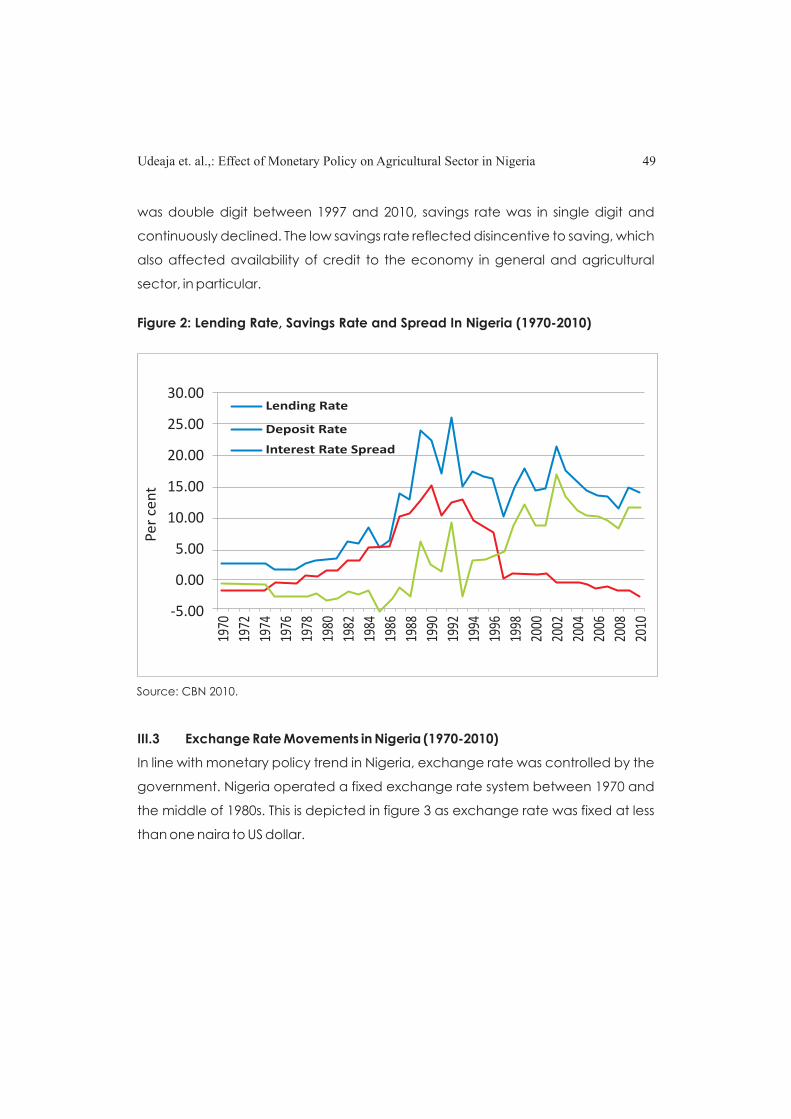
was double digit between 1997 and 2010, savings rate was in single digit and
continuously declined. The low savings rate reflected disincentive to saving, which
also affected availability of credit to the economy in general and agricultural
sector, in particular.
III.3 Exchange Rate Movements in Nigeria (1970-2010)
In line with monetary policy trend in Nigeria, exchange rate was controlled by the
government. Nigeria operated a fixed exchange rate system between 1970 and
the middle of 1980s. This is depicted in figure 3 as exchange rate was fixed at less
than one naira to US dollar.
Udeaja et. al.,: Effect of Monetary Policy on Agricultural Sector in Nigeria 49P
er
cen
t
30.00
25.00
20.00
15.00
10.00
5.00
0.00
-5.00
1970
1972
1974
1976
1978
1980
1982
1984
1986
1988
1990
1992
1994
1996
1998
2000
2002
2004
2006
2008
2010
Lending Rate
Deposit Rate
Interest Rate Spread
Figure 2: Lending Rate, Savings Rate and Spread In Nigeria (1970-2010)
Source: CBN 2010.

The fixed exchange rate system led to the overvaluation of the Naira relative to the
major global currencies, resulting in distortions in the domestic economy as imports
become relatively cheaper. The development resulted in balance of payments
disequilibrium and subsequent capital flight and a drain on the external reserves. In
1980, following the oil glut, and the global depression and the mounting external
debts that followed, it became imperative for the country to move away from the
pegged exchange rate system to a flexible one. In 1986, under the Structural
Adjustment Programme (SAP), Nigeria adopted the flexible exchange rate system,
which allowed the exchange rate to be determined by the market forces. The
adoption of the flexible exchange rate system, however, led to the depreciation of
the currency from N0.8938/US$1 in 1985 to N2.0206/U$1 in 1986.
Various reforms were carried out in an attempt to achieve the objectives of
exchange rate policy including the Second-Tier Foreign Exchange Market (SFEM)
which metamorphosed from the Foreign Exchange Market (FEM), the
Autonomous Foreign Exchange Market (AFEM), Inter-Bank Foreign Exchange
Market (IFEM), the Retail Dutch Auction System (rDAS) and the Wholesale Dutch
50 Central Bank of Nigeria Economic and Financial Review June 2014
160.0000
140.0000
120.0000
100.0000
80.0000
60.0000
40.0000
20.0000Nai
ra p
er u
nit o
f Dol
lar
Exchange Rate 19
70
1972
1974
1976
1978
1980
1982
1984
1986
1988
1990
1992
1994
1996
1998
2000
2002
2004
2006
2008
2010
Exchange
Figure 3: Exchange Rate in Nigeria (1970-2010)
Source: CBN 2010.

Auction System (WDAS). The application of each arrangement also produced a
significant effect on the exchange rate as the naira exchange rate continued to
depreciate gradually. By 1991, the exchange rate had depreciated to
N9.9095/US$1 and sharply to N17.2984/US$1 in 1992. The rate further depreciated
to N92.6934/US$1 in 1999, N102.1052/US$1 in 2000, N132.1470/US$1 in 2005 before
reaching a height of N150.66/US$1 in 2010.
IV. Monetary Policy Objectives and Agricultural Sector in Nigeria
Generally, the objective of monetary policy is the same both in the developed and
developing economies. The objectives of monetary policy include, among others,
the achievement of price stability; attainment of full employment; attainment of
balance of payments equilibrium; achievement of rapid economic growth and
maintenance of exchange rate stability. However, as observed by Ajayi and Ojo
(2006), there seems to be very scanty empirical studies on the objectives of
monetary policy in Nigeria. This study therefore deviates in its analysis and
concentrates more in reviewing monetary policy objectives over the years and its
effect on the agricultural sector in Nigeria.
While earlier analysis in this respect has discussed monetary policy performance,
using two broad epochs, this study splits the two epochs into short intervals and
proceeds with the analysis. Following from Ajayi and Ojo (2006) analysis, the
current study splits the periods as follows.
Phase 1: 1960 - 1969
The early part of this period was characterised by maintaining sound currency. The
Central Bank of Nigeria was still at its infancy with limited power to fully administer a
sound monetary policy. The then newly issued Nigerian currency suffered
acceptability and convertibility as it was still tied to the British pounds and sterling.
The objective of monetary policy was that of accumulation of external reserves.
But after 1962, emphasis was put on development as policy objective strived to
ensure adequate supply of credit to the economy without creating inflationary
pressures (Ajayi and Ojo, 2006). The increase in credit greatly benefited the
agricultural sector as credit to agriculture increased, leading to an increase in
Udeaja et. al.,: Effect of Monetary Policy on Agricultural Sector in Nigeria 51

agricultural output. Consequently, the contribution of agriculture to real total GDP
stood at 55.4 per cent in 1965 (see table 1). The later part of 1965 witnessed the
policy of credit rationing in the form of guidelines that placed ceilings on the ability
of commercial banks to create credits. This led to a sharp fall in credit allocated to
agriculture from 25.3 per cent in 1965 to 2.0 per cent in 1970 (see table 3). However,
the later part of the period witnessed the outbreak of civil war, which redirected
the objective of monetary policy. In effect, monetary policy was redirected at
financing the war as government pursued the policy of cheap borrowing to
execute the war.
Phase 2: 1970- 1974
This period is usually referred to as the inflationary era. This is because the period
was characterised by rising inflationary pressures from the disruption of the
economic activities by the civil war. Monetary policy stance was expansionary in
line with the Federal Government's 3Rs- Reconstruction, Resettlement and
Reconciliation programme. By 1975 inflation had become a serious national issue
as inflation rate reached about 34 per cent from about 3 per cent in 1972 (Ajayi
and Ojo, 2006). To stem such tide in inflation, the CBN introduced the sectoral
distribution of credit policy, in which cheap credits were allowed to the more
productive sectors of the economy, in particular the agricultural sector. Interest
rate was also kept at relatively low levels at about 7.0 per cent. Other direct
monetary measures to control the indiscriminate credit creation by commercial
banks included: credit ceilings; selective credit controls; cash requirements; and
special deposits. Following this monetary tightening policy, credit to agriculture fell
from 25.3 per cent in 1965 to 2.6 per cent in 1975. The share of agriculture in total
real GDP also fell from 44.7 per cent in 1970 to 28.1 per cent in 1975.
Phase 3: 1975-1985
The period was also characterised by direct control of monetary policy instruments
by the Government through the monetary authorities. The main objective of
monetary policy in this period was the promotion of rapid and sustainable
52 Central Bank of Nigeria Economic and Financial Review June 2014
economic growth. To achieve this objective, the CBN continued with its direct
control and rationing of credit policy as loans and advances were directed to the
preferred sectors of the economy. The ceiling on individual banks' credit to the
preferred sectors was fixed at 30-40 per cent of banks aggregate loans and
advances in the early 1980s, but was reduced to 7 per cent in 1985 (Ajayi and Ojo,
2006). Agriculture being the core component of the preferred sector benefited
from this policy as share of credit to the sector increased from 2.6 per cent in 1975 to
10.8 per cent in 1985. Its share of the total real GDP also rose from 20.6 per cent in
1980 to 32.7 per cent in 1985. However, beginning from early 1980s, there was
shortfall in oil receipts which made it increasingly difficult for the Government to
perform its fiscal responsibilities. The government therefore resorted to borrowing
from the Central Bank to finance the existing huge deficits. The development had
adverse implications for monetary management. The monetary control
framework, which relied heavily on credit ceilings and selective credit controls,
increasingly failed to achieve the set targets as their implementation became less
effective (CBN,2007).
Phase 4: 1986-2010
Beginning from 1986, the monetary policy formulation and objectives assumed a
different dimension. The deregulation of the economy following the
implementation of SAP in 1986 brought with it monetary policy changes. SAP was
introduced as a result of the crash in the international oil market prices and the
resultant deteriorating economic conditions in the country. SAP was designed to
achieve the following objectives, namely:
i. To achieve fiscal balance and balance of payments viability by altering
and restructuring the production and consumption patterns in the
economy;
ii. To rationalise the role of the public sector and accelerate the growth
potentials of the private sector;
iii. To restructure and diversify the productive base of the economy so as to
reduce dependency on the oil sector; and
iv. To embark on privatization and commercialisation of the economy aimed
Udeaja et. al.,: Effect of Monetary Policy on Agricultural Sector in Nigeria 53

at promoting industrial efficiency, among others.
The main strategies of the programme were the deregulation of external trade
and payments arrangements, the adoption of a market-determined exchange
rate for the naira, substantial reduction in complex price and administrative
controls and more reliance on market forces as a major determinant of economic
activity.
Under the SAP framework, the objective of monetary policy was directed at
inducing the emergence of a market-oriented financial system for effective
mobilisation of financial savings and efficient resource allocation. To achieve this,
monetary policy variables such as interest rate and exchange rate were liberalised
thereby allowing banks to determine deposit and lending rates based on market
conditions. The main instrument of the market-based framework was the open
market operations (OMO). OMO was complemented by reserve requirements
and discount window operations. Meanwhile, the deregulation of the interest rate
had positive effects on the agricultural sector in Nigeria. First, following the
deregulation of interest rate, credit allocation to agricultural sector rose from 10.8
per cent in 1985 to 16.2 per cent in 1990 and further to 22.0 per cent in 1995.
Second, agricultural share of the total real GDP also experienced some sort of
revival as it rose from 20.6 per cent in 1980 to 31.5 per cent in 1990 and further to 34.2
per cent in 1995 (see table 1).
Another major development was that the sector-specific credit allocation targets
were compressed into four sectors in 1986, and subsequently to two in 1987 and by
1996, all mandatory credit allocation mechanisms were abolished. Both
commercial and merchant banks were subjected to equal treatment since their
operations were found to produce similar effects on the monetary process. In 2002,
the CBN commenced a medium-term monetary policy framework with the
primary aim of achieving price and exchange rate stability by minimising the
problem of time inconsistency and over-reaction due to temporary shocks. The
Dutch Auction System (DAS) of foreign exchange management was
reintroduced. This action engendered relative stability, and stemmed further
54 Central Bank of Nigeria Economic and Financial Review June 2014

depletion of reserves. However, the financial system was characterised by rapid
expansion in monetary aggregates, particularly during the second half of 2000,
influenced by the monetisation of enhanced oil receipts. Consequently, monetary
growth accelerated significantly, exceeding policy targets by substantial margins.
Savings rate and the inter-bank call rates fell generally due to the liquidity surfeit in
the banking system and the spread between deposit and lending rates widened
(see figure 2 for trend). The high lending rates constricted credit to agriculture as
commercial banks loans to the sector fell from 22.0 per cent of total commercial
banks credit in 1995 to 8.5 per cent of total credit in 2000 and fell further to 3.5 per
cent of total credit in 2005.
In 2003, another monetary policy measure was designed aimed at promoting a
stable macroeconomic environment and achieve a non-inflationary output
growth rate of 5 per cent. In pursuit of its developmental effort, the Central Bank, in
collaboration with the Bankers' Committee, established the Small and Medium
Industries Equity Investment Scheme (SMIEIS). Credit delivery to real sector was
encouraged through the SMIEIS and an incentive of lower Cash Reserve
Requirement (CRR) regime was prescribed for those banks that increased their
credit allocation to the real sector by 20 per cent or more. Moreover, the Bank
provided guarantees for agricultural loans under the Agricultural Credit
Guarantee Scheme (ACGS). In spite of these schemes, commercial banks credit
to agriculture continued to plunge as shown in table 3.
Following the global financial crisis of 2008/2009, the Central Bank of Nigeria
recognised the need to accompany the objective of maintaining price stability
with financial system stability. The thrust of monetary policy during the period
centered on providing adequate liquidity in the banking system. The Monetary
Policy Rate (MPR) was upheld as an anchor to all other short-term market rates. The
major instrument of the monetary policy was the Open Market Operations (OMO)
conducted through Treasury Bills auction in the primary market. This policy
continued into 2010 as monetary policy objective aimed at ensuring price and
Udeaja et. al.,: Effect of Monetary Policy on Agricultural Sector in Nigeria 55

financial stability.
V. The Government's Interventions in Agricultural Sector through the
Central Bank of Nigeria
The role of government through the Central Bank of Nigeria (CBN) in the
agricultural sector has always been in term of financing. Over the years, the
Nigerian government through the central bank has instituted various schemes
aimed at enhancing the development of agriculture in Nigeria. Among these
schemes are:
i. Sectoral Credit Allocation: Prior to 1996, direct measures such as selective
credit control, credit ceilings, administered interest rate and exchange
rate, cash requirements and special deposits were frequently used to
regulate the flow of credit in the economy by the CBN. Cheap credits were
allowed to the more productive (priority) sectors of the economy and in
particular the agricultural sector. Interest rate was also kept at relatively low
levels at about 7.0 per cent.
ii. Nigeria Agricultural Co-operative and Rural Development Bank (NACRDB):
The bank was established in 1972, but renamed Nigerian Agricultural and
Cooperative Bank (NACB) in 1978. In 2000, it was merged with the People's
Bank of Nigeria (PBN) to become Nigerian Agricultural Cooperative and
Rural Development Bank Limited (NACRDB). The bank is jointly owned by
the Central Bank of Nigeria (40 per cent) and the Federal Ministry of
Finance (60 per cent). The bank was purposefully set up to promote growth
in the quantity and quality of credit to agriculture, including lending to
individuals and state governments. It was also aimed at directly making
loans available and strengthening local micro finance banks, which
deliver credit at the local community level. It was also to improve storage
facilities and promote marketing of farm produce.
iii. Agricultural Credit Guarantee Scheme Fund (ACGSF): Agricultural Credit
Guarantee Scheme Fund (ACGSF) was established in 1977 under the
56 Central Bank of Nigeria Economic and Financial Review June 2014

management of the Central Bank of Nigeria (CBN), which handles the day-
to-day operations of the Scheme. The Federal Government holds 60 per
cent of the total shares, while, Central Bank of Nigeria holds the remaining
40 per cent of the shares. The main objective of the Fund was to guarantee
credit facilities extended to farmers by banks up to 75 per cent of the
amount in default net of any security realized. Agricultural activities for
which loans can be guaranteed by the Fund include: establishment or
management of plantation for the production of rubber, oil palm, cocoa,
coffee, tea and similar crops; production of cereal crops, tubers, fruits of all
kinds, cotton, beans, groundnuts, sheanuts, benniseed, vegetables, pine-
apples, bananas and plantains; animal husbandry, including poultry,
piggery, cattle rearing and the like, fish farming and fish capture;
processing activities such as cassava to gari, oil palm fruit to palm oil and
kernel, groundnut to groundnut oil, etc and farm machinery and hire
services.
iv. The Self-Help Group Linkage Programme: The Self-Help Group Linkage
programme was launched in 1991 by the government via the Central Bank
of Nigeria. It became operational in 1992. This Scheme was a product
under the Agricultural Credit Guarantee Scheme Fund (ACGSF). The aim of
the Self-Help Group Linkage Banking is to inculcate the culture of savings
and banking habit in group members as well enable them to build up
resources for financing their farm projects without recourse to bank
borrowing on the long-run. Under this Scheme, farmers are encouraged to
form themselves into groups of between 5 and 15 on the basis of common
purpose and undertake regular savings with a partner bank of their choice.
After 6 months of regular savings, the group can apply for loan, which is
given to them in multiples of the balance in their savings account at the
time of the application for the loan.
v. The Trust Fund Model (TFM): The Trust Fund Model was established to
enhance credit supply to the agricultural and rural sectors of the economy.
Udeaja et. al.,: Effect of Monetary Policy on Agricultural Sector in Nigeria 57

Under the Model, oil companies, State and Local Governments and Non-
Governmental Organisations (NGOs) are required to place funds in trust
with lending banks to augment the small group-savings of the farmers as
security for agricultural loans. The Trust Fund secures 25 per cent or more of
the intended loans of the prospective borrowers, the farmers' savings
secure another 25 per cent while the ACGSF guarantees 75.0 per cent of
the remaining 50.0 per cent, thereby leaving the lending bank with a risk
exposure of only 12.5 per cent.
vi. The Interest Drawback Programme (IDP): The Interest Drawback
Programme was developed as an interest rate management framework
under the ACGSF to reduce effective borrowing rates without the
complication of introducing dual interest rate regime or contradicting the
existing deregulation policy of the government. Under the IDP, farmers will
borrow from lending banks at market-determined rates, but the
Programme will provide interest rebate of a determined percentage to
them where the loans are repaid as and when due. The IDP is funded jointly
by the Federal Government and the Central Bank of Nigeria in the ratio of
60:40. The IDP is regarded as a dedicated fund for interest drawback on
agricultural loans or IDP Fund and separated from the ACGSF capital.
vii. Small and Medium Industries Equity Investment Scheme (SMIEIS): The
Government through the Central Bank of Nigeria established the Small and
Medium Industries Equity Scheme (SMIEIS) in 2001. The Scheme requires
banks to set aside 10 per cent of their before-tax profit annually to be
invested in equity in small and medium industries. The specific objectives of
the scheme include: to facilitate the flow of funds for the establishment of
new Small and Medium Investment (SMI) projects; stimulate economic
growth, develop local technology and generate employment; develop
and package viable industries with Nigerian entrepreneurs; provide
venture capital and management that would spearhead the restructuring
and financing of the small and medium scale industries (SMI). The range of
58 Central Bank of Nigeria Economic and Financial Review June 2014

activities of which funds shall be applied are those in the real sector, which
include: Agro-Allied; Information Technology and Communication;
Manufacturing; Educational Establishments; Services; Tourism and Leisure;
Solid Minerals; and Construction.
viii. Refinancing and Rediscounting Scheme (RRF): In 2002, the Refinancing
and Rediscounting Scheme (RRF) was launched by the Central Bank of
Nigeria. The RRF was developed to serve as an incentive for attracting
loans to medium to long-gestation real sector projects such as agriculture,
semi-manufacturing and manufacturing, exploration and exploitation of
solid minerals, and Information Technology (IT). It is a window and an
incentive meant to provide temporary relief to deposit money banks,
which may face liquidity problems as a result of committing their resources
to medium to long-term funding of real sector activities. To farmers, it offer
concessionary interest rate on term loans for agricultural investments and
afford them to conveniently repay the loans as well as to make profits.
ix. Agricultural Credit Support Scheme (ACSS): In 2006, the Federal
Government through the Central Bank of Nigeria (CBN) with the active
support and participation of the Bankers' Committee established the
Agricultural Credit Support Scheme (ACSS) with the total fund portfolio of
N50 billion. The main aim of the Scheme was to develop the agricultural
sector of Nigeria by providing credit facilities to farmers at single digit
interest rates to enable them make use of the untapped potentials in the
sector, thereby reducing the cost of food products and inflation rate. This
will consequently increase the production of agricultural exports and
diversify the revenue base as well as increase the foreign exchange
earnings of the country. The Scheme at its inception was billed to grant
loans to deserving farmers at 14 per cent interest, but farmers who are able
to pay back the loan within the stipulated period enjoy a rebate of 6 per
cent, resulting to 8 per cent effective interest rate paid by farmers.
Udeaja et. al.,: Effect of Monetary Policy on Agricultural Sector in Nigeria 59

x. Commercial Agriculture Credit Scheme (CACS) Fund: As part of its
developmental role, the Central Bank of Nigeria (CBN), in conjunction with
the Federal Ministry of Agriculture and Water Resources (FMA&WR),
established the N200 billion Commercial Agriculture Credit Scheme
(CACS) fund in April 2009. The Funds are being channeled through the
deposit money banks to farmers with interest rate not exceeding 9 per cent
and maturity period not more than 7 years. The overall objective of the
Scheme is to provide finance for the country's agricultural value chain
comprising production, processing, storage and marketing. The specific
objectives of the Scheme include:
·To speed up the development of the agricultural sector in Nigeria
by providing credit facilities to large-scale commercial farmers at a
single digit interest rate (precisely at 9 per cent);
·To enhance food security in the country by increasing food supply
and effecting lower agricultural products prices, thereby ensuring
low food inflation;
·To reduce the cost of credit in agricultural production to enable
farmers exploit the untapped potentials of the sector; and
·To increase total output, generate employment, diversify Nigeria's
revenue base, raise the level of foreign exchange earnings and
provide input for manufacturing and processing on a sustainable
basis.
VI. Methodology
The study adopted the Auto- Regressive Distributed Lag (ARDL) model for its
analysis. One advantage of the Bound Testing approach is that it can be applied
irrespective of whether variables in the model are purely I(0), purely I(1) and
mutually co-integrated. This avoids the pre-testing problems associated with
standard co-integration test such as the classification of variables into I(0) and I(1).
Moreover, the test is relatively efficient in small and finite sample data size.
However, before estimating the ARDL model, the study tested for unit root and co-
60 Central Bank of Nigeria Economic and Financial Review June 2014
Udeaja et. al.,: Effect of Monetary Policy on Agricultural Sector in Nigeria 61
integration among variables in the model. The unit root test is conducted using the
Augmented Dickey Fuller (ADF) test proposed by Dickey and Fuller (1979) and
Phillips-Perron (PP) test proposed by Phillips and Perron (1988) with intercept only.
VI.1 Empirical Model
Theoretical literature established three major transmission channels through which
monetary policy affects agricultural output. These include interest rate channel,
credit channel and exchange rate channel. The study considered these
endogenous variables in addition to two non-policy variables, which also affect
the agricultural sector.
Based on this theoretical exposition, the empirical model was formulated and
expressed as:
AGOUT= f (LEN, CBLA, EXCH, INF, GXPA) (1)
Where:
AGOUT = Agricultural GDP
LEN = Lending Rate
CBLA = Commercial Banks Loans and Advances to Agriculture in Nigeria
EXCH = Exchange Rate
INF = Inflation Rate
GXPA = Government Expenditure in Agriculture in Nigeria
Given the time series nature of the data used, the unit root procedure requires
estimating the following ADF and PP equations:
ADF Estimation:
Where:
0 1
1
k
t t t i ti
Y a Y Y Ug ib- -=
D=++D+å
1--=D ttt YYY
(2)
is the first difference of series Y ;t
211 --- -=D ttt YYY is the first difference of Yt-1

62 Central Bank of Nigeria Economic and Financial Review June 2014
Where:
á ë ã, â and ñ are parameters to be estimated; U and å are stochastic error 0, 0, i, t, t
terms.
In both ADF and PP tests, the null hypothesis of non-stationarity (presence of unit
root) is accepted if ã = 0 and ñ = 1, respectively, while the null hypothesis of non-
stationarity is rejected if ã <0 and ñ <1, respectively.
Following from Pesaran, Shin and Smith (2001), the Error Correction Model (ECM) of
the unrestricted Auto Regressive Distributed Lag (ARDL) equation based on
equation (1) is specified as follows:
Where:
U is the white noise error term.t
The first part of the right hand side of equation (4) with parameters á to á 1 5
represents the long-run dynamics of the model and the second part with
parameters to represents the short-run dynamics of the model.
The ARDL approach involves testing first for the co-integration relationship among
the variables in the model. In specific term, the bounds test involves estimating
equation (4) and then testing the null hypothesis (H ) of no long-run relationship 0
against the alternative hypothesis (H ) that there is a long-run relationship. That is: a
H : á =á =á =á =á =0, against the alternative hypothesis: H : á≠ á≠ á≠ á≠0 1 2 3 4 5 a 1 2 3 4
á≠0. The calculated F-statistic is then compared with the critical values given in 5
Pesaran et. al.,(2001). If the computed F-statistics exceeds the upper critical value,
the null hypothesis of no long-run relationship can be rejected. On the other hand,
if the F-statistics falls below a lower critical value, then the null hypothesis cannot be
rejected. Lastly, if the F-statistics lies between the upper and lower critical values, it
? ?
0 1 .t t tY Ylre-=++ (3)
0 1 1 2 1 3 1 4 1 5 1
1
k
t t t t t t i t ii
AGOUT LEN CBLA EXCH INF GXPA AGOUTaa a a a a b- - - - - -=
D =+ + + + + +Då
0 0 0 0 0
k k k k k
i t i i t i i t i i t i t i ti i i i i
LEN CBLA EXCH INF GXPA Uj d w g ip- - - - -= = = = =
+D+D +D +D+D +ååå åå(4)
ipib
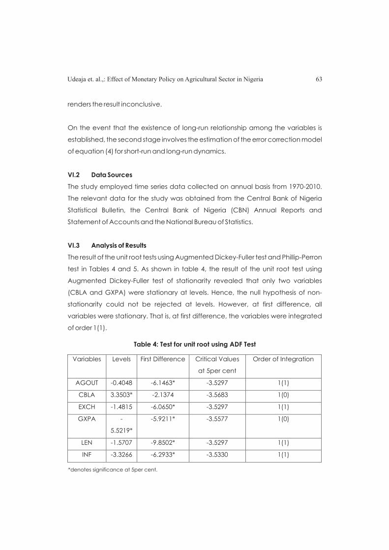
renders the result inconclusive.
On the event that the existence of long-run relationship among the variables is
established, the second stage involves the estimation of the error correction model
of equation (4) for short-run and long-run dynamics.
VI.2 Data Sources
The study employed time series data collected on annual basis from 1970-2010.
The relevant data for the study was obtained from the Central Bank of Nigeria
Statistical Bulletin, the Central Bank of Nigeria (CBN) Annual Reports and
Statement of Accounts and the National Bureau of Statistics.
VI.3 Analysis of Results
The result of the unit root tests using Augmented Dickey-Fuller test and Phillip-Perron
test in Tables 4 and 5. As shown in table 4, the result of the unit root test using
Augmented Dickey-Fuller test of stationarity revealed that only two variables
(CBLA and GXPA) were stationary at levels. Hence, the null hypothesis of non-
stationarity could not be rejected at levels. However, at first difference, all
variables were stationary. That is, at first difference, the variables were integrated
of order 1(1).
Udeaja et. al.,: Effect of Monetary Policy on Agricultural Sector in Nigeria 63
Table 4: Test for unit root using ADF Test
Variables Levels First Difference Critical Values
at 5per cent
Order of Integration
AGOUT -0.4048 -6.1463* -3.5297 1(1)
CBLA 3.3503* -2.1374 -3.5683 1(0)
EXCH -1.4815 -6.0650* -3.5297 1(1)
GXPA -
5.5219*
-5.9211* -3.5577 1(0)
LEN -1.5707 -9.8502* -3.5297 1(1)
INF -3.3266 -6.2933* -3.5330 1(1)
*denotes significance at 5per cent.

Table 5 also showed the test of unit root using Phllip-Perron test. As the result
showed, only one variable (GXPA) was stationary at levels. Just as in the ADF test
above, the null hypothesis of non-stationary of the series could not be rejected. All
variables were, however, stationary when the series was differenced once.
From the unit root tests conducted above, it was revealed that the variables were
integrated of order 1(1), which suggested the presence of co-integration
relationship among them. To establish this long-run relationship, the bounds test co-
integration analysis was carried out. The result of the bounds test was reported in
table 6. From the result obtained, the calculated F-Statistics value of 1251.49 was
greater than the upper- bound critical value of 4.90 at 1 per cent level. Since the F-
Statistics value was greater than the upper-bound critical value, the null hypothesis
of no co-integration was rejected; hence there was co-integration (long-run
relationship) among the variables in the model.
Since it was established that there was a long-run relationship among the variables
in the model, we proceeded to estimate the error correction model for short-run
estimates. The results of the short-run dynamics from the error correction model
presented in Table 7 showed that exchange rate and government expenditure on
agriculture had significant short-run effect on agricultural output in Nigeria. The
64 Central Bank of Nigeria Economic and Financial Review June 2014
Table 5: Test for unit root using PP test
Variables
Levels
First-diff
Critical
Value at 5per
cent
Order of
Integration
AGOUT
-0.3609
-6.1503*
-3.5297
I(1)
CBLA
-2.0655
-28.7995*
-3.5297
I(1)
EXCH -1.4815 -6.0650* -3.5297 I(1)
GXPA -5.5334* -31.5919* -3.5297 I(0)
LEN -2.8068 -10.0030* -3.5297 I(1)
INF -3.1857 -11.5234* -3.5297 I(1)
*denotes significance at 5 per cent.

coefficient of exchange rate was positive, showing that a shock to exchange rate
(i.e. depreciation) will generate positive reaction to increased agricultural
production for export. Precisely, the high elasticity of exchange rate is indicative of
the strong sensitivity of agricultural output to exchange rate shock. An
appreciation of the exchange rate will increase competitiveness of agricultural
export and attract investment in the agricultural sector. Similarly, the positive sign
of the coefficient of Government expenditure on agriculture showed that there
was a short-run positive effect of Government spending on agricultural output in
Nigeria. This implied that a 1 per cent increase in Government expenditure in
agriculture leads to 1.08 per cent increase in agriculture productivity in Nigeria,
other things being equal. The result was in line with those obtained by Udoh (2011)
and Udoh et. al.,(2012).
The adjusted R-Squared showed that the explanatory variables have explained 52
per cent of the total variations in agricultural output in Nigeria. The F-statistics
(13.81) also showed that the explanatory variables collectively were significant in
explaining short-run changes in agricultural output in Nigeria. The Durbin-Watson
value of 1.91 showed there was no autocorrelation in the model. Meanwhile, the
coefficient of the error correction term is negative in line with a priori expectation
but however, not statistically significant. Thus, there is a slow rate of adjustment to
equilibrium.
Udeaja et. al.,: Effect of Monetary Policy on Agricultural Sector in Nigeria 65
Table 6: Results from Bounds test
Bounds Test:
F-statistic
(p-value)
1251.49
(0.02)
Critical bounds (1per
cent)#:
lower and upper 3.60 and 4.90
Decision: Co-integration
#Unrestricted Intercept and Unrestricted trend (k=6) from Pesaran et. al.,(2001).
The full regression result is presented in Table A1 in the appendix.

VII. Policy Recommendations and Conclusion
The study examined the effect of monetary policy on agricultural output in Nigeria
for the period 1970 to 2010, utilising monetary policy variables such as commercial
banks credit to agricultural sector, exchange rate, lending rate and two non-
policy variables, which were Government expenditure and inflation rate. As earlier
stated, it is believed that monetary policy has real and nominal effect on the
overall economic activities and, hence agricultural sector only in the short-run and
medium–run, but has no significant effect in the long-run. The argument in this
regard is that the fundamental forces that shape outcome and, hence forces that
determine the behaviour of output in the agricultural sector are believed to be
consequences of non-monetary conditions. Following from the above debate,
the study was undertaken to examine whether monetary policy has effect on the
outcomes of agricultural output in Nigeria.
The result obtained showed that monetary policy through exchange rate channel
had significant positive effect on agricultural output in Nigeria. The results also
showed that Government expenditure on agricultural sector had a positive and
significant impact on output of agriculture in Nigeria.
66 Central Bank of Nigeria Economic and Financial Review June 2014
Table 7: Error Correction Model
Dependent Variable: ?AGOUT
Explanatory
variables
Coefficient t-statistic Probability
Constant 4854.75 2.67 0.01
?EXCH(-4) 905.33 4.58 0.0001
?GXPA(-3) 1.08 5.94 0.0000
ECM(-1) -0.009 -0.14 0.88
Adjusted R-squared
0.52
F-statistic
13.81
Diagnostic Tests: Serial Correlation [0.16 (0.85)], ARCH [0.039 (0.84)], Heteroscedasticity [0.18 (0.99)]
Functional Form (RAMSEY RESET) [0.12 (0.88)

To boost agricultural productivity in Nigeria, the following policy recommendations
are relevant:
i There is need for the Government to continue to invest in the
agricultural sector in Nigeria through its direct spending in the sector.
Spending may take the form of infrastructural development,
establishment of research centres, provision of farm inputs at subsidised
rates, and direct provision of credits to farmers through specialised
agencies.
ii There is need to maintain a sound exchange rate policy that will lead to
increased agricultural output in the economy. The current exchange
rate appears overvalued. The study has demonstrated that some level
of depreciation should be permitted to help boost agricultural exports.
However, excessive depreciation should be avoided as it can affect
importation of essential farm inputs such as equipments and
machineries needed by farmers.
iii Farmers should be given easy access to credit so as to boost their
productivity. Commercial banks should be mandated to lend to
farmers at a very low interest rate. The existing small and medium scale
investment scheme fund and the microfinance arrangements should
be properly managed and made functional as they can prove to be
veritable sources of finance to farmers.
Udeaja et. al.,: Effect of Monetary Policy on Agricultural Sector in Nigeria 67

References
Abayomi F, (2006). “An Overview of Nigerian Agricultural Sectors”, Journal of
Agricultural Economics, 8 (3): 7-16.
Ajaiyi,S. and O. Ojo (2006). Money and Banking: Analysis and Policy in the Nigerian
Context. Ibadan: Daily Graphics Nigeria Ltd.
Ardeni, P. G. and J. Freebairn (2002). The Macroeconomics of Agriculture. In: Gardner,
B. and Rausser, G.C. (eds.). Handbook of Agricultural Economics. Vol. 2A.
Amsterdam: North-Holland, 1455-1485.
Asfaha, T. and A. Jooste (2006). “The Agricultural Input Elasticity of Rural Urban
Migration in South Africa”, Agrekon, Vol. 45 (1): 89- 105.
Athukorala, P. C. (1998). “Interest Rate, Saving and Investments. Evidence from India”,
Oxford Development studies, 26(2), 153-169.
Bakucs, L. and I. Ferto (2005). “Monetary Impacts and Overshooting of Agricultural
Prices in an Open Economy” Paper prepared for the XIth International Congress
of the European Association of Agricultural Economists (EAAE), Copenhagen,
Denmark, August 24-27, 2005.
Barbhart, S. W. (1989). “The Effect of Macroeconomic Announcements on Commodity
Prices”, American Journal of Agricultural Economics, Vol. 71: 389-403.
Bessler, D. A. (1984). Relative Prices and Money: A Vector Auto Regression on Brazilian
Data, American Journal of Agricultural Economics, Vol. 65: 25-30.
Central Bank of Nigeria (2007). Annual Reports and Statement of Accounts, December,
2007.
Chambers, R. G. (1984). “Agricultural and Financial Market Interdependence in the
Short-run”. American Journal of Agricultural Economics. 66(1), pp. 12-24.
Chambers, R. G. and R. E. Just, (1980). A Critique of Exchange Rate Treatment in
Agricultural Trade Model. American Journal of Agricultural Economics, Vol. 62:
255- 259.
Cho, G., M. Kim and W. Koo (2004). “The Relative Impact of National Monetary Policies
and International Exchange Rate on long-term Variations in Relative Agricultural
Prices”, Agribusiness and Applied Economic Report, No. 528. North Dakota State
University.
Chuku A. C. (2009). “Measuring the Effects of Monetary Policy Innovations in Nigeria: A
68 Central Bank of Nigeria Economic and Financial Review June 2014

Structural Vector Autoregressive (SVAR) Approach”, African Journal of
Accounting, Economics, Finance and Banking Research, Vol. 5. No. 5, PP. 112-
129.
Devadoss, S. and W. Meyers (1987). Relative Prices and Money: Further Results for the
United States, American Journal of Agricultural Economics, Vol. 69: 838-842.
Dickey, D. A. and W. A. Fuller (1979). “Distribution for Estimators for Autoregressive Time
Series with a Unit Root”, Journal of the American Statistical Society, Vol. 74,
pp.427-431.
Eyo, E. O. (2008). “Macroeconomic Environment and Agricultural Sector Growth in
Nigeria”, World Journal of Agricultural Sciences 4 (6), PP. 781-786
Frankel, J. A. (1986). Expectations and Commodity Price Dynamics: The Overshooting
Model, American Journal of Agricultural Economics, Vol. 68: 344-348.
Friedman, M. (1969). The Optimum Quantity of Money and Other essays. Chicago:
Aldine.
Jingan, M. L. (2004). Monetary Economics. Delhi: Vrinda Publications Ltd.
Kliesen, K. and W. Poole (2000). Agriculture Outcomes and Monetary Policy Actions:
Kissin’ Cousins? ASU Agriculture-Business Conference, ASU Convocation Centre
Jonesboro, Arkansas, February 16, 2000.
Lai, C., S. Hu and V. Wang (1996). Commodity Price Dynamics and Anticipated
Shocks. American Journal of Agricultural Economics, Vol. 78: 982-990.
Nwosa, P. I. and M. O. Saibu (2012). “The Monetary Transmission Mechanism in Nigeria:
A Sectoral Output Analysis”, International Journal of Economics and Finance,
Vol. 4, No. 1, PP. 204-212.
Oden, D. (2003). US Agricultural Policy: The 2002 Farm Bill and WTO Doha Round
Proposal. TMD Discussion Paper No 109, International Food Policy Research
Institute, Washington, DC.
Omojimite, B. U. (2012). Institutions, Macroeconomic Policy and Growth of the
Agricultural Sector in Nigeria, Global Journal of Human Social Science, Vol. 12,
Issue1, January, 2012.
Onoja, A. O. and A. C. Agumagu (2009). “Econometric Modelling of the Effects of
Economic Policies on Food Output in Nigeria under Obasanjo’s Administration”,
Udeaja et. al.,: Effect of Monetary Policy on Agricultural Sector in Nigeria 69
Journal of Sustainable Development in Africa, Vol.11, No 1, PP. 98-112.
Orden, D. (1986). “Agriculture, Trade and Macroeconomics: The U.S. Case”, Journal of
Policy Modelling, 8:1 (Spring). pp. 27-51.
Orden, D. and P. Fackler (1989). “Identifying Monetary Impacts on Agricultural Prices in
VAR Models”, American Journal of Agricultural Economics, 71(2), pp. 495-502.
Phillips, P. and P. Perron (1988). “Testing for Unit Roots in Time Series Regression”,
Biometrika, 75, 335-346.
Robertson, J. and D. Orden (1990). Monetary Impacts on Prices in the Short and Long-
run: Some Evidence from New Zealand. American Journal of Agricultural
Economics, Vol. 72: 160-171.
Saghaian, S. H., M. R. Reed and M. A. Merchant (2002). “Monetary Impacts and
Overshooting of Agricultural Prices in an Open Economy”, American Journal of
Agricultural Economics, Vol. 84: 91-103.
Saibu, M. O. and I. P. Nwosa (2011). “Effects of Monetary Policy on Sectoral Output
Growth in Nigeria”, Journal of Economics and Behavioural Studies, Vol. 2, No. 6,
pp. 245-254.
Schuh, G. E. (1974). “The Exchange Rate and U.S. Agriculture”, American Journal of
Agricultural Economics, 56(1) pp. 1-13.
Tweeten, L. G. (1980). Macroeconomics in Crisis: Agriculture and Underachieving
Economy. American Journal of Agricultural Economics 62, 853-860.
Udah, E. B. (2009). “Monetary Policy and Macroeconomic Management: A Simulation
Experiment”, Global Journal of Social Sciences Vol. 8, No. 1, Pp. 1-13.
Udoh, E. (2011). “An Examination of Public Expenditure, Private investment and
Agricultural Sector Growth in Nigeria: Bounds Testing Approach”, International
Journal of Business and Social Science, Vol. 2, No. 13, PP. 285-292.
Udoh, E., E. Udeaja and F. Ebong (2012). ‘‘Public Expenditure, Foreign Direct Investment
and Agricultural Sector Growth in Developing Countries: The Case of Nigeria’’.
Middle Eastern Finance and Economics, Issue 17, PP. 59-69.
Pesaran, M. H., Y. Shin and R. J. Smith (2001). “Bounds Testing Approaches to the
Analysis of Level Relationships”,Journal of Applied Econometrics, Vol. 16, pp. 289-
326.
70 Central Bank of Nigeria Economic and Financial Review June 2014

Uniamikogbo S. O. and A. I. Enoma (2001). The Impact of Monetary Policy on
Manufacturing Sector in Nigeria: an Empirical Analysis. The Nigerian Journal of
Economic and Financial Review, 3 (2): 37-45.
Udeaja et. al.,: Effect of Monetary Policy on Agricultural Sector in Nigeria 71
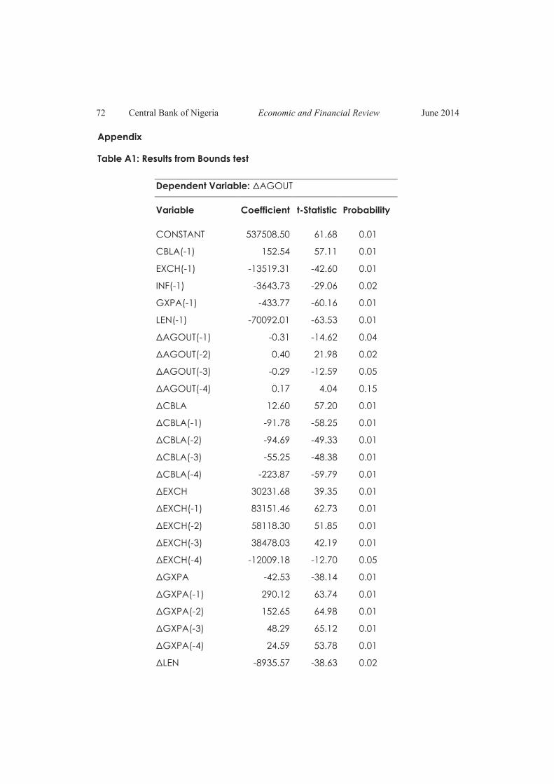
72 Central Bank of Nigeria Economic and Financial Review June 2014
Appendix
Table A1: Results from Bounds test
Dependent Variable: ÄAGOUT
Variable Coefficient t-Statistic Probability
CONSTANT 537508.50 61.68 0.01
CBLA(-1) 152.54 57.11 0.01
EXCH(-1) -13519.31 -42.60 0.01
INF(-1) -3643.73 -29.06 0.02
GXPA(-1) -433.77 -60.16 0.01
LEN(-1) -70092.01 -63.53 0.01
ÄAGOUT(-1) -0.31 -14.62 0.04
ÄAGOUT(-2) 0.40 21.98 0.02
ÄAGOUT(-3) -0.29 -12.59 0.05
ÄAGOUT(-4) 0.17 4.04 0.15
ÄCBLA 12.60 57.20 0.01
ÄCBLA(-1) -91.78 -58.25 0.01
ÄCBLA(-2) -94.69 -49.33 0.01
ÄCBLA(-3) -55.25 -48.38 0.01
ÄCBLA(-4) -223.87 -59.79 0.01
ÄEXCH 30231.68 39.35 0.01
ÄEXCH(-1) 83151.46 62.73 0.01
ÄEXCH(-2) 58118.30 51.85 0.01
ÄEXCH(-3) 38478.03 42.19 0.01
ÄEXCH(-4) -12009.18 -12.70 0.05
ÄGXPA -42.53 -38.14 0.01
ÄGXPA(-1) 290.12 63.74 0.01
ÄGXPA(-2) 152.65 64.98 0.01
ÄGXPA(-3) 48.29 65.12 0.01
ÄGXPA(-4) 24.59 53.78 0.01
ÄLEN -8935.57 -38.63 0.02

Udeaja et. al.,: Effect of Monetary Policy on Agricultural Sector in Nigeria 73
ÄLEN(-1) 48776.17 62.00 0.01
ÄLEN(-2) 64992.42 63.05 0.01
ÄLEN(-3) 59336.52 69.92 0.01
ÄLEN(-4) 37615.63 63.66 0.01
ÄINF 80.01 1.69 0.33
ÄINF(-1) 3685.46 36.80 0.02
ÄINF(-2) 2737.44 40.14 0.02
Ä INF(-3) 2377.59 37.50 0.02
ÄINF(-4) 2543.94 49.93 0.01
R-squared 0.99
Adjusted R-squared 0.99
Durbin-Watson
stat 2.49
F-statistic 626.52
Prob(F-statistic) 0.03
Bounds Test:
F-statistic
(p-value)
1251.49
(0.02)
Critical bounds (1per
cent)#:
lower and upper 3.60 and 4.90
Decision: Co-integration
#Unrestricted Intercept and Unrestricted trend (k=6) from Pesaran et al (2001).
Table A2: Error Correction Model
Dependent Variable: ÄAGOUT
Variable
Coefficient
t-Statistic
Probability
CONSTANT
4854.75
2.67
0.01
ÄEXCH(-4) 905.33 4.58 0.0001
ÄGXPA(-3) 1.08 5.94 0.0000
ECM(-1) -0.009 -0.14 0.88

74 Central Bank of Nigeria Economic and Financial Review June 2014
R-squared 0.56
Adjusted R-
squared 0.52
Durbin-Watson stat 1.91 F-statistic
13.81
Diagnostic Tests: Serial Correlation [0.16 (0.85)], ARCH [0.039 (0.84)], Heteroscedasticity [0.18 (0.99)]
Functional Form (RAMSEY RESET) [0.12 (0.88).

An Autoregressive Distributed Lag (ARDL) Approach to the Oil Consumption and
Growth Nexus: Nigerian Evidence
Inuwa N., H. M. Usman and A. M. SaiduAbstract
This study attempted to examine the relationship between oil consumption, carbon
emission and economic growth in Nigeria covering the period 1980-2011. The study applied
Dickey-Fuller Generalised Least Square (DF-GLS) unit root test and autoregressive distributed
lag (ARDL) bound test approach to co-integration. The bond test results revealed a long-run
equilibrium relationship among oil consumption, carbon emission and economic growth.
The result also showed a positive and statistically significant impact of oil consumption on
economic growth. The coefficient of error correction term in the ARDL model was
statistically significant, indicating that the adjustment process by which long-run equilibrium
is restored after a shock is very fast. In conclusion, oil consumption played an important role
in the economic growth of Nigeria, thus efforts to conserve oil will have a negative
repercussions on economic growth. Therefore, Nigeria should endeavour to overcome the
*
* Inuwa Nasiru, Haruna Modibbo Usman and Abubakar Mohammed Saidu are staff of the
Department of Economics, Faculty of Arts and Social Sciences, Gombe State University, P.M.B 127,
Gombe. The usual disclaimer applies.
I. Introduction
il serves as one of the critical factor in promoting and sustaining
economic growth. Despite Nigeria's proven reserve of crude oil of 37.2
billion barrels as at the end of 2010, the tenth largest in the world and the Osecond largest in Africa behind Libya, the largest amount of that consumed is
imported (Sambo, 2010). It is worth noting that the share of oil in total export value
rose from less than 1 per cent in 1958 to a peak of 97 per cent in 1984 and has not
been less than 90 per cent since then. In the first half of 1990, it accounted for over
95 per cent of total exports and its share of GDP had ranged between 25 and 30
per cent in recent years.
However, the linkage of carbon emission and growth is also closely related to the
Central Bank of Nigeria Economic and Financial Review Volume 52 No. 2 June 2014 75
Keywords: Oil consumption, Economic growth, ARDL, Nigeria

relationship between oil consumption and carbon emission as combating oil use
will, on one hand, reduce the level of emission and on the other might affect
economic growth in a negative manner (Ozturk and Uddin, 2012). With the recent
rapid industrialisation, increased population and significant change in life style, the
threat of global warming, climate change and environmental degradation
particularly the unprecedented increase in CO emissions (Nwosa, 2013) became 2
visible. It is, therefore, important to examine the relationship among oil
consumption, CO emissions and economic growth by bringing out the policy 2
implications on the economy.
Unlike the previous studies conducted on the relationship between energy
consumption and economic growth in Nigeria (e.g., Ebohon, 1996: Odularo, 2008;
Olusegun, 2008; Omotor, 2008; Odularo and Okonkwo, 2009; Dantama, Zakari,
and Inuwa, 2012; Dantama and Inuwa, 2012; Olumuyiwa, 2012; Nwosa, 2013; and
Olufemi and Olalekan, 2013), the relationship between oil consumption and
economic growth has not been deeply examined.
To the best of the authors' knowledge, no study that focuses on the relationship
between oil consumption and economic growth with respect to Nigeria has been
carried out. Thus, the purpose of this paper is to examine the effect of oil
consumption and CO emissions on economic growth and to also suggest 2
appropriate policy recommendation. The rest of the paper is organised as follows.
Section 2 presents the brief literature review whereas, Section 3 discusses the
nature of the data and the proposed econometric methods adopted. Section 4
presents the empirical results, while the last Section concludes the paper.
II. Literature Review and Theoretical Framework
It is worth-noting that mainstream economic theories do not explicitly specified a
relationship among energy consumption, CO emissions, and economic growth. A 2
number of studies have examined the relationship between energy consumption
and economic growth, between environmental pollution and economic growth
and their policy implications (Tiwari, 2011). This line of research focuses on the
76 Central Bank of Nigeria Economic and Financial Review June 2014

Environmental Kuznets Curve (EKC) or what is also termed the Carbon Kuznets
Curve (CKC) hypothesis. The higher economic growth rates pursued by
developing countries, the greater the consumption of an increasing quantity of
commercial energy, which comes at the cost of ignoring technologies that are
more efficient. Thus, there is controversy as to whether energy consumption is a
stimulating factor, or is itself a result of economic growth. The increased share of
CO emissions in the atmosphere that is a product of the unbridled use of fossil fuels 2
has negative impacts on natural systems (Tiwari, 2011).
However, empirical studies were conducted to examine the relationship between
oil consumption, carbon emissions and economic growth. Zou and Chau
(2006),Yoo (2006), Aktas and Yilmaz (2008), Bhusal (2010); and Farooq and Ullah
(2011) applied Johansen maximum likelihood co-integration technique and error
correction model to study the short- and long-run relationships between oil
consumption and economic growth for China, Korea, Turkey, Nepal and Pakistan,
respectively. The estimation results revealed a bi-directional causal short and long-
run equilibrium relationship between oil consumption and economic growth.
Other studies by Park and Yoo (2013), Yazdan and Hossein (2013) and Lim, Lim, and
Yoo (2014) also applied the Johansen maximum likelihood co-integration test
technique and Granger causality test based vector error correction model
(VECM) to study causal relationship between oil consumption and economic
growth for Malaysia, Iran and Philippines, respectively. The studies concluded that
a long-run equilibrium relationship existed between oil consumption and
economic growth. The short-run causality revealed bidirectional causality
between oil consumption and economic growth. The long-run causality results
further revealed bidirectional causality between oil consumption and economic
growth. A similar study by Stambuli (2014) for Tanzania during the period 1972-2010
revealed a long-run equilibrium relationship between oil consumption, oil prices,
and economic growth. The Granger causality test revealed a unidirectional
causality running from oil consumption to oil prices, and from economic growth to
oil consumption. The results therefore justified conservation hypothesis.
Inuwa et.al.,: An ARDL Approach to the Oil Consumption and Growth Nexus 77

Using autoregressive distributed lag (ARDL) bounds test, Fuinhas and Marques
(2012) examined the relationship between oil consumption and economic growth
in Portugal during the period 1965-2009. The results established a long-run
equilibrium relationship between oil consumption and economic growth. It further
revealed bidirectional causality between oil consumption and economic growth
in both the short-run and long-run.
However, on the basis of panel data, Narayan and Wong (2009) applied panel co-
integration developed by Pedroni and Panel Granger causality test to identify the
determinants of oil consumption for 6 Australian states and Territory over the period
1985-2006. The results showed the existence of long-run relationship among oil
consumption, oil prices, and income. Further, oil prices had positive but statistically
insignificant impact on oil consumption, while income had a positive and
significant effect on oil consumption; meaning that 1 per cent increase in per
capita income would lead to an increase in per capita oil consumption by 0.2 per
cent. The causality test results suggested unidirectional causality running from
income to both oil prices and oil consumption in both the short-and long-run.
Similarly, Pourhosseingholi (2013) applied Pedroni panel co-integration technique,
full modified ordinary least square (FMOLS) and Granger causality test based on
vector error correction model (VECM) to examine the causal relationship between
oil consumption and economic growth for the OPEC member countries during the
period 1980-2011. The study concluded that a long-run equilibrium relationship
existed between oil consumption and economic growth while the Granger
causality test results presented a bi-directional causality between oil consumption
and economic growth.
Al-mulali (2011) applied Engle and Granger, Kao co-integration techniques and
panel Granger causality test to investigate the impact of oil consumption on
economic growth for MENA countries over the period 1980-2011. The results
showed that CO emission and oil consumption had long-run equilibrium 2
relationship with economic growth. Furthermore, Granger causality test results
reveal bidirectional causality between oil consumption, CO emission and 2
78 Central Bank of Nigeria Economic and Financial Review June 2014

economic growth in both short and long-run.
Behmiri and Manso (2012) applied Engle-Granger two-stage co-integration
technique and panel Granger causality tests to investigate the long-run and
causal relationships between crude oil consumption and economic growth,
covering the period 1976-2009 for 27 OECD countries. The results suggested the
existence of long-run relationships among crude oil consumption, crude oil price
and GDP proxied for economic growth. The panel Granger causality results
showed two-way relationships for both short- and long-run, thereby disputing
crude oil conservation hypothesis as any increase or decrease in crude oil
consumption would adversely affect the economic growth of the OECD countries.
Another recent study by Chu (2012) employed Bootstrap panel Granger Causality
test to study the direction of causality between oil consumption and economic
growth for 49 countries over the period 1970-2010. The results were classified into
growth, conservation, neutrality and feedback hypotheses. The direction of
causality between oil consumption and output justified neutrality hypothesis for 24
countries, growth hypothesis for 5 countries, conservation hypothesis for 13
countries as well as feedback hypothesis for 7 countries.
However, using a cross-country study of 42 countries to compare oil consumption
and economic efficiency of advanced, developing and emerging economies,
Halkos and Tzeremes (2011) applied Data Envelopment Analysis (DEA) and
generalised method of moments (GMM) over the period 1986-2006. The findings
showed that advanced economies had much higher turning points compared to
developing and emerging economies. Moreover, oil consumption increased
economic efficiency for all the countries. Finally, the GMM estimates revealed the
presence of an inverted U-shaped relationship between countries economic
efficiency and oil consumption, with statistically significant estimates.
Ozturk and Uddin (2012) applied Johansen maximum likelihood test approach to
co-integration and Granger causality based on vector error correction model
Inuwa et.al.,: An ARDL Approach to the Oil Consumption and Growth Nexus 79

(VECM) to investigate the causal relationship between energy consumption,
carbon emissions and economic growth for India during the period 1971-2007. The
results showed bidirectional causality between energy consumption and
economic growth. Also, there was unidirectional causality running from energy
consumption to carbon emission.
III. Methodology
III.1 Data
The data used consisted of annual time series of Real Gross Domestic Product
(RGDP), oil consumption and CO emissions for Nigeria 1980 to 2011. The data on 2
RGDP was obtained from the Central Bank of Nigeria Statistical Bulletin, while data
on oil consumption were obtained from the International Energy Statistics and
data on CO emissions were obtained from World Development Indicators (2013). 2
RGDP was used as proxy for economic growth, following the work of Zou and Chau
(2006), Oil consumption was used as petroleum consumption. It was expressed as
thousands of barrels per day as done by Yoo (2013) and Fuinhas and Marques
(2013). A carbon dioxide emission was employed as those emissions stemming
from the burning of fossil fuels and the manufacture of cement. The choice of this
variable was justified as done by Lim, Lim and Yoo (2014) and Ozturk and Uddin
(2012).
III.2 Unit Root Test
The ARDL bounds testing approach to co-integration can be applied irrespective
of whether the variables are I(0), I(1) or fractionally co-integrated However, in the
presence of I(2) variables the computed F-statistics provided by Pesaran, Shin, and
Smith (2001) become invalid. This is because the bounds test is based on the
assumption that the variables should be I(0) or I(1). Therefore, the implementation
of unit root tests in the ARDL procedure is necessary to ensure that none of the
variables is integrated of order two i.e. I(2) or beyond. For this purpose, the study
uses the conventional DF-GLS unit root tests.
.
80 Central Bank of Nigeria Economic and Financial Review June 2014
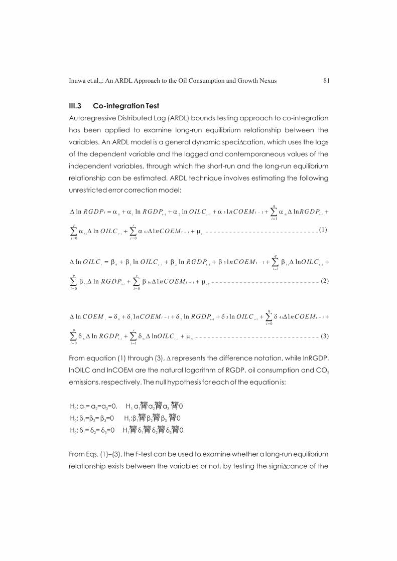
III.3 Co-integration Test
Autoregressive Distributed Lag (ARDL) bounds testing approach to co-integration
has been applied to examine long-run equilibrium relationship between the
variables. An ARDL model is a general dynamic speci?cation, which uses the lags
of the dependent variable and the lagged and contemporaneous values of the
independent variables, through which the short-run and the long-run equilibrium
relationship can be estimated. ARDL technique involves estimating the following
unrestricted error correction model:
From equation (1) through (3), ? represents the difference notation, while lnRGDP,
lnOILC and lnCOEM are the natural logarithm of RGDP, oil consumption and CO2
emissions, respectively. The null hypothesis for each of the equation is:
H : á = á =á =0, H á≠á≠á ≠00 1 2 3 1: 1 2 3
H : â =â = â =0 H :â≠ â≠ â ≠00 1 2 3 1 1 2 3
H : ä = ä = ä =0 H≠ ä≠ ä≠ ä≠00 1 2 3 1 1 2 3
From Eqs. (1)–(3), the F-test can be used to examine whether a long-run equilibrium
relationship exists between the variables or not, by testing the signi?cance of the
Inuwa et.al.,: An ARDL Approach to the Oil Consumption and Growth Nexus 81
0 1 1 2 1 4
5 1
3 1
1
6 (1)0 0
ln ln ln 1 ln
ln 1
t t i t i
i t i t
q
t t
i
p r
i t i
i i
RGDP RGDP OILC nCOEM RGDP
OILC nC OEM
aa a a a
a a m
- - -
-
-
=
- -----------------------------
= =
D =+ + + +D +
D + D +
å
å å
0 1 1 2 1 4
5 2
3 1
1
6
0 0
ln ln ln 1 ln
ln 1
t t t i t i
i t i t
q
t
i
p r
i t i
i i
O ILC OILC RG DP nC O EM O ILC
RG D P nC O EM
bb b b b
b b m
- - -
-
-
=
- (2)---------------------------
= =
D =+ + + +D +
D + D +
å
å å
0 1 2 1 1
5 6 3
1 3 4
0
0 1
ln 1 ln ln 1
ln ln
t t t
i t i i t i t
q
t i t i
i
p r
i i
COEM nCOEM RGDP OILC nCOEM
RGDP OILC
dd d d d
d d m
- -
- -
- -
=
= =
D =+ + + +D +
D +D +
å
å å (3)-------------------------------

lagged level variable. The computed F-statistics for co-integration are denoted as
F (RGDP/OILC,COEM), F (OILC/RGDP,CEOM), and F (COEM/RGDP RGDP OILC CEOM
OILC)for each equation, respectively. Pesaran, Shin and Smith (2001) tabulated
two sets of critical values. The ?rst set of critical values is called lower-bounds critical
values, and the second set of critical values is known as upper bounds critical
values. According to Pesaran, Shin, and Smith (2001), the null hypothesis of no co-
integration is rejected if the calculated F-statistic is more than the upper-bound
critical values. On the other hand, if the calculated F-statistic is less than the lower-
bound critical values, we cannot reject the null hypothesis, and hence the
variables are not co-integrated. Finally, the decision about co-integration is
inconclusive if the calculated F-statistic falls between the lower and upper-bound
critical values.
IV. Empirical Results
This section consists preliminary analyses (where results of the of unit root tests and
co-integration tests are presented and discussed); estimation results (where the
regression results are presented and discussed); and post-estimation analysis
(where the model diagnostics are presented and discussed).
IV.1 Preliminary Analyses
The results of the unit root test are presented in Table 1. The DF-GLS test results
indicate that all the variables; i.e. RGDP, oil consumption, and CO emissions, are 2
stationary after first differencing. Thus, the necessary condition for the application
of the bounds test is justified.
82 Central Bank of Nigeria Economic and Financial Review June 2014
Table 1 Unit Root Tests
Variable DF-GLS test at Level DF-GLS at first Difference
RGDP -0.225930 -2.246696**
OILC -1.362379 -4.487645***
COEM -1.276135 -4.933902***
Source: authors' computations ***and** indicates level of significance at 1per cent and 5per cent

Inuwa et.al.,: An ARDL Approach to the Oil Consumption and Growth Nexus 83
IV.2 Estimation Results
The results of the bounds test approach to co-integration are reported in
The bounds test indicated that co-integration was only present when RGDP was
the dependent variable. This was because F (RGDP/OILC, COEM) was 6.1294 RGDP
higher than the upper bound critical value at the 5per cent critical value.
However, the bounds test indicated that the test was inclusive when OILC was
taken as dependent variable because F (OILC/RGDP, COEM) fell within the OILC
lower and upper bound critical value. As for COEM as dependent variable, the
F (COEM/RGDP, OILC,) was lower than the lower bound critical value at the 5 COEM
per cent level. Therefore, there was co-integration when Real GDP was treated as
the dependent variable.
The results of the estimated long-run coefficients were presented in Table 3. The
estimated coefficients of the long-run relationship showed that oil consumption
has a positive and significant impact on real GDP; a proxy for economic growth.
Therefore, a unit increase in oil consumption led to approximately 1.98 unit
increase in real GDP in Nigeria. However, the coefficient of CO emissions was not 2
significant.
Table 2.
Table 2: Bounds Test Results
F-Statistic Critical Values at
5per cent
Lower bound Upper bound
FRGDP (RGDP/OILC,COEM) =6.1294 2.9666 4.2347
FOILC (OILC/RGDP,COEM) =4.0594
FCOEM (COEM/RGDP,OILC) =1.0528
Source: authors’ computations.
Table 3: Results of Estimated Long-run Coefficients
Regressor Coefficient Standard error T-ratio [p-value]
Dependent variable; RGDP
OILC 1.9784 .011481 172.3301[.000]
COEM -.22164 .21095 -1.0507[.303]
Source: authors’ computations.

The results of the short-run dynamic coefficients associated with the long-run
relationship obtained from the ECM equation were reported in Table 4. The sign of
the short-run dynamic impact was maintained to the long-run. The error correction
coefficient estimated at -0.12832 (0.002) was highly significant; it had the correct
sign and implied a high speed of adjustment to equilibrium after a shock.
Approximately 12.8 per cent of disequilibria from the previous year's shock was
restored in the current year.
IV.3 Post-estimation Analysis
Table 5 presented diagnostics test of the estimated ARDL model. The model
passed all diagnostic tests. There was no evidence of serial correlation and the
model was well specified, based on their probability values. Similarly, the battery of
diagnostic tests for heteroscedasticity and normality of the residuals, did not find
any signi?cant evidence of departures from standard assumptions.
84 Central Bank of Nigeria Economic and Financial Review June 2014
Table 4: Error Correction Representation for the Selected ARDL Model
Regressor Coefficient Standard error T-ratio [p-value]
Dependent variable:
?RGDP
?OILC .25388 .073960 3.4326 [.002]
?CEOM -.028441 .024283 -1.1713[.252]
ECM (-1) -.12832 .037532 -3.4190[.002]
Source: authors’ computations.
Table 5: Diagnostics Test
Test Statistics LM test
Serial Correlation CHSQ(1) =1.8068[.179]
Functional Form CHSQ(1) =0.021169[.884]
Normality CHSQ(2) =0 .80823[.668]
Heteroscedasticity CHSQ(1) =0 .89441[.344]
Source: authors’ computation.

V. Conclusion
This study examined the relationship among oil consumption, CO emissions, and 2
economic growth in Nigeria during the period 1980–2011 using autoregressive
distributed lag (ARDL) bounds testing approach to co-integration. Empirical results
showed that there was long-run equilibrium relationship among oil consumption,
CO emissions, and economic growth. Also, oil consumption had positive and 2
statistically significant impact on economic growth. Furthermore, the coefficient of
error correction term in the ARDL model was statistically significant and was
correctly signed.
Thus, oil consumption could be considered as one of the leading determinants of
economic growth in the short-run as well as in the long-run. The basic premise for
this may be that the enormous use of oil, mostly in the industry sector, had directly
pushed the economy. Therefore, policy makers in Nigeria should take into account
that implementing oil conservation policies will affect economic growth
negatively since it has been found to have positive impact on economic growth.
Inuwa et.al.,: An ARDL Approach to the Oil Consumption and Growth Nexus 85

References
Aktas, C. and V. Yilmaz (2008). “Causal Relationship between oil Consumption and
Economic Growth in Turkey”, Kocaeli Universitesi Sosyal Bilimler Enstitusu
Dergisi, 15, 45-55.
Al-mulali, U. (2011). “Oil Consumption, CO emission, and Economic Growth in the 2
MENA Countries”, Energy, 36, 6165-6171.
Behmiri, N. B. and J. R. P. Manso (2012a). “Crude Oil Conservation Policy Hypothesis
in OECD Countries: A Multivariate Panel Granger Causality Tests”, Energy, 43,
253-260.
Behmiri, N. B. and J. R. P. Manso (2012b). “Does Portuguese Economy Support
Crude Oil Conservation Hypothesis?”, Energy, 45, 628-634.
Bhusal, T. P. (2010). “Econometric Analysis of Oil Consumption and Economic
Growth in Nepal”, Economic Journal of Development Issues, 11&12, 135-143.
Chu, H. (2012). “Oil Consumption and Output: What Causes What? Bootstrap
Panel Causality for 49 Countries”, Energy Policy, 51, 907-915.
Dantama, Y. U. and N. Imuwa (2012). “A Granger Causality Examination between
Energy Consumption and Economic Growth in Nigeria”, Journal of
Economics, Commerce and Research (JECR), 2(2), 14 – 24.
Dantama, Y. U., A. Y. Zakari, and N. Inuwa (2012). “Energy Consumption-Economic
Growth Nexus: An Empirical Assessment Based on ARDL Bounds Test
Approach”, European Scientific Journal, 8(12), 141-157.
Ebohon, O. J. (1996). "Energy, Economic Growth and Causality in Developing
Countries: A Case Study of Tanzania and Nigeria", Energy Policy,
24(5), 447-53.
Farooq, M. B. and S. Ullah (2011). “Sectoral Oil Consumption and Economic Growth
in Pakistan: An ECM Approach”, American Journal of Scientific Industrial
Research, 2(2), 149-156.
Fuinhas, J. A. and A. C. Marques (2012). “An ARDL Approach to the Oil and Growth
Nexus: Portuguese”, Energy Sources, Part B: Economics, Planning and Policy,
7(3), 282-291.
86 Central Bank of Nigeria Economic and Financial Review June 2014

Halkos, G. E. and G. N. Tzemeres (2011). “Oil Consumption and Economic
Efficiency: A Comparative Analysis of Advanced, Developing and Emerging
Economies”, Ecological Economics, 70,1354-1362.
Lim, K. M., S. Y. Lim and S. H. Yoo (2014). “Oil Consumption, CO Emission and 2
Economic Growth: Evidence from Philippines”, Sustainability, 6, 967-979.
Narayan, P. K. and P. Wong (2009). “A Panel Data Analysis of the Determinants of
Oil Consumption: The Case of Australia”, Applied Energy, 86, 2771-2775.
Nwosa, P. I. (2013). “Long-run and Short-run Relationship between Fuel
Consumption and Economic Growth in Nigeria”, Journal of Sustainable
Development in Africa, 15(4), 130-142.
Odularu, G. O. and C. Okonkwo (2009). “Does Energy Consumption Contribute to
Economic Performance? Empirical Evidence from Nigeria”, Journal of
Economics and International Finance, 1(2), 044-058.
Olufemi, S. M. and J. A. Olalekan (2013). “Energy Consumption, Carbon Emission,
and Economic Growth: Implications for Energy Policy and Climate
Protection in Nigeria”, International Conference on Energy Policies and
Climate Protection, 339-345.
Odularu, G. O. (2008). “Crude Oil and the Nigerian Economic Performance”, Oil
Gas Business, http://www.ogbus.ru/eng/
Olusegun, O. A. (2008). “Energy consumption and Economic Growth in Nigeria: A
Bounds Testing Co-integrative Approach”, Journal of Economic Theory, 2(4),
118-123.
Olumuyiwa, O. S. (2012). “Long-Run Relationship Between Energy Consumption
and Economic Growth: Evidence from Nigeria”, IOSR Journal of Humanities
and Social Sciences, 3(3), 40-51.
Ozturk, I. and G. S. Uddin, (2012). “Causality among Carbon Emissions, Energy
Consumption and Growth in India”, Economic Research, 25(3), 752-775.
Omotor, D. G. (2008). “Causality between Energy Consumption and Economic
Growth in Nigeria”, Pakistan Journal of Social Sciences, 5 (8), 827 -835.
Pesaran, H. M., Y. Shin and R. J. Smith (2001). “Bounds Testing Approaches to the
Analysis of Long-run Relationships”, Journal of Applied Econometrics, 16, 289-
Inuwa et.al.,: An ARDL Approach to the Oil Consumption and Growth Nexus 87

326.
Pourhosseingholi, N. (2013). “Causality Between Oil Consumption and Economic
Growth in OPEC Countries: A Panel Co-integration Approach”, Asian
Economic and Financial Review, 3(12), 1642-1650.
Park, S. Y. and S. H. Yoo (2013). “The Dynamics of Oil Consumption and Economic
Growth in Malaysia”, Energy Policy, 1-6.
Sambo, A. S. (2010). “Renewable Energy Development in Nigeria”, A Paper
Presented at the World Future Council/strategy Workshop on 21 Renewable
Energy, Accra, Ghana.
Stambuli, B. B. (2014). “Oil Consumption and Economic Growth Nexus in Tanzania
Co-integration Causality Analysis”, International Journal of Academic
Research in Economic and Management Sciences, 3(2), 113-123.
Tiwari, A. K. (2011). “Energy Consumption, CO2 Emissions and Economic Growth:
Evidence from India”, Journal of International Business and Economy, 12(1),
85-122.
Yazdan, G. F. and S. S. M. Hossein (2013). “Causality Between Oil Consumption and
Economic Growth in Iran: An ARDL Testing Approach”, Asian Economic and
Financial Review, 2(6), 678-686.
World Bank (2013). World Development Indicators 2013, CD ROM version.
Washington, DC.
Yoo, S. H. (2006). “Oil Consumption and Economic Growth: Evidence from Korea”,
Energy Sources, Part B: Economics, Planning, and Policy, 1(3), 235-243.
Zou, G. and K. W. Chau (2006). “Short and Long-run Effects Between Oil
Consumption and Economic Growth in China”, Energy Policy, 34, 3644-3655.
88 Central Bank of Nigeria Economic and Financial Review June 2014

SUBMISSION OF MANUSCRIPT TO CBN ECONOMIC AND FINANCIAL REVIEW
1. Three (3) hardcopies and a softcopy of the original manuscript should be
addressed to the:
Editor-in-chief
CBN Economic and Financial Review
Research Department
Central Bank of Nigeria
P.M.B.0187, Garki, Abuja
The softcopy of the papers can also be submitted via email as electronic
document, preferably Microsoft word document to either of the following
email addresses: [email protected]; [email protected].
The article should not be more than 20 pages on A4 size paper and should be
typed double-spaced with a margin of 1.5 inches on all sides. The manuscript
must be accompanied with a letter of submission written in English.
Submission of a paper is assumed to imply that its contents represent original
and unpublished work and is not under consideration elsewhere for
publication. Normally, the review process is expected to take not more than
three months. There is neither a submission charge nor page fee. A return
address (postal/email) should be indicated.
2. Papers may be accepted or returned for specified revisions. A paper is
expected to be published approximately six months from the date of
acceptance.
3. Comments on published article/notes and reviews of up to 2,000 words will
also be considered for publication. Notes deal with relevant topics not
meeting full length articles. Reviews may be about articles published
recently by this journal or elsewhere. A copy of the review/comments should
be sent to the articles' author for clarification of any points or
Inuwa et.al.,: An ARDL Approach to the Oil Consumption and Growth Nexus 89

misunderstandings.
4. All submitted manuscripts are referred to an Editorial Board comprising of an
in-house editorial committee and external referees. All comments by the
referees will be sent to the author(s) together with a decision of the Editorial
Board.
5. The purpose and scope of the article should be clearly stated in an abstract
summarising the article's essential points. The abstract should be typed on a
separate page and should be between 80-100 words in length. In addition,
the JEL classification code (s) as well as keywords should be clearly indicated
on the abstract page.
6. The author's institutional affiliation and necessary background information
on the article should appear at the foot of the first page. Footnote to the text
should be listed at the end, followed by the list of references
7. References for quotations or statements should be in parentheses in the text,
not as notes. E.g. Hess (1906:20) or Cagan (1958) or Majer (1975:35). Where
more than three authors are invol.ved, cite senior author and use et al., E.G.
Johnson et al. (1988).
8. Citations listed under the reference sections must begin on a new page. All
entries must be typed double-spaced, listed alphabetically by last name of
senior author and chronologically for two or more articles by the same
author. The typed layout must conform to the following examples:
Nnanna, O. J. (2003). “Promoting Savings and Investment Culture for
National Development.” CBN Economic and Financial Review. Vol.
41. No. 3 pp. 1-10
Oresotu, F. O. and C. N. O. Mordi (1992). “The Demand for Money Function in
Nigeria: An Empirical Investigation.” CBN Economic and Financial
90 Central Bank of Nigeria Economic and Financial Review June 2014

Review. Vol.30, No.1 pp.32-69.
Croxton, F. E.; F. E. Cowden; and S. Klein, (1968). Applied General Statistics.
London: Sir Isaac Pitman and sons.
9. All tabular materials should be separated from the text in a series of tables
numbered consecutively in Arabic numerals preferably in Microsoft Excel.
Each table should be typed double-spaced and identified by a short
descriptive at the top. Notes for table should be at the bottom of each table,
before the source, and marked by lower case superscript letters.
Appropriately placed tables should be indicated in the text.
10. Diagrams, graphs, charts, etc. must be separated from the text and clearly
drawn in black ink on a white paper with all axes clearly positioned. They
should be submitted in a form suitable for reproduction without redrawing,
preferably in camera-ready artwork.
11. Where mathematical equations and formulae are used, they should be
typed clearly. Notations, exponents, etc, which are simple to reproduce
should be used. The equations should be numbered consecutively in Arabic
numerals. The full mathematical workings necessary for justifying each step
of the argument should accompany all the articles of a mathematical
nature. This is meant to assist the reviewers and will not be published.
Inuwa et.al.,: An ARDL Approach to the Oil Consumption and Growth Nexus 91