Embed Size (px)
Citation preview
j ,UNj
CENTER FOR RADAR ASTRONOMY -r
STANFORD ELECTRONICS LABORATORIES /DEPARTMENT OF ELECTRICAL ENGINEERING
SSTANFORD UNIVERSITY. STANFORD, CA 94305 SU-SEL-78-•2
-4 - iOIFT ALGORITHMS-
•' ANALYSIS AND IMPLEMENTATION,
iL.
S. Shank ,rtNarayan
3 /M. J.jNarasimhaAllen M.JPeterson i4 L OiKmZUi"
(.i May .78 rI
Technical $epat, o. 3606-12 25 1978J
Prepared under
Joint Service n n oat,Contract N14-75-C-0 1
; 5 014
DFT ALGORITHMS -
ANALYSIS AND IMPLEMENTATION
by
S. Shankar Narayan
M. J. Narp.,imhaAllen M. Peterson
May 1978
Prepared under
Joint Services Engineering ProjectContract N00014-75 C-0601
-A.Ii
ACKNOWLEDGEMENTS
The authors wish to thank Kok Chen for useful discussion they had with
him during the course of this study. They are also pleased to acknowledge
Irene Stratton for her meticulous typing of this report.
This work was supported by Joint Services Engineering Project Contract
NOOI14-75-C-0601.
1..
ABSTRACT
Efficient algorithms for 11 and 13-point DFT's are presented. A more
efficient algorithm, compared to earlier published versions, for the computa-
tion of 9-point DFT is also included. The effect of arithmetic roundoff in
implementing the prime factor and the nested algorithms for computing DFT with
fixed point arithmetic is analyzed using a statistical model. Various aspects
of the prime facc -, the nested and the radix-2 FFT algorithms are compared.
A processor-based hardware implementation of the prime factor algorithm is
discussed.
{K
CONTENTS
I. INTRODUCTION ....... ....... ......................... I
II. DFT ALGORITHMS FOR COMPOSITE N ......... ................ 3
1. Fast Fourier Transform ......... .................. 3
2. Prime Factor Algorithm ......... .................. 5
3. Nested Algorithm ....... ... ..................... 7
III. SHORT LENGTH DFT ALGORITHMS ........ ................. 11
IV. FIXED POINT PFA AND WFTA ERROR ANALYSIS ... ........... .... 20
1. WFTA ................... . ..... .............. 22
2. PFA ........... ........................... ... 25
V. COMPARISON OF DFT ALGORITHMS ..... ................. ... 29
1. Arithmetic Operations ........ ................... 29
2. Memory Requirement ....... ..... .................. 31
3. Programming Complexity ..... .................. ... 33
4. Effect of Finite Wordlength Arithmetic ..... .......... 33
VI. A HARDWARE IMPLEMENTATION OF PFA .... ............... .... 35
VII. CONCLUSION ......... .......................... ... 42
VIII. REFERENCES ......... .......................... ... 43
APPENDIX A: Program for 120-point DF1 Computation by PFA .... ...... 45
r1
CHAPTER I
INTRODUCTION
The discrete Fourier transform (OFT) of a sequence xk$ k 0, 1, ... 9
N - 1, is defined as [1]
N-i
Xn XkWN , n = 0, 1, ... , N-i (1.1)k=O
where WN = exp (-j 27T/N) . It is an invertible transformation and the sequence
xk can be recovered using the following inverse OFT (IDFT) relation:
N-i
Xk N j_ W1fl , k = 0, I, ... , N-l (1 .2)n:O
Many digital signal processing systems employ the OFT for a variety of
applications. The design and implementation of digital filters, spectral ana-
lysis of signals, and detection of targets from radar echoes are a few examples.
As a result, there is a continued interest in finding increasingly sophisticated
algorithms for computing the DFT.
The direct evaluation of Xn in Eqation (1 1) requires about N2 multi-
plications and additions (hereafter these two arithmetic operations are referred
to simply as "operations"). If N is a composite number, however, the compu-
tational burden can be reduced by employing one of the three following algorithms:
(a) Fast Fourier transform (FFT) algorithm
(b) Prime factor algorithm (PFA)
(c) Nested or Winograd Fourier transform algorithm (WFTA)
2
The factors of N have to be relatively prime for the PFA and the WFTA,
while no such constraint is imposed in the case of the FFT. These algo-
rithms are briefly discussed in Chapter II.
Efficient algorithms to find the DFT of short sequences are needed to
obtain the transform of longer sequences by the PFA and the WFTA. An
efficient procedure for deriving the Short length DFT algorithms, when the
transform length is a prime or a prime power, is discussed in [2]. Algo-
rithms for several short length transforms derived using this method, are
given in [3] and [4]. In Chapter III this procedure is briefly explained,
and efficient algorithms for 9, 11 and 13-point DFT's are presented. The
short length DFT algorithms given in [3] are also listed.
The DFT algorithms can be either programmed on general purpose digital
computers or implemented directly by special purpose hardware. In either
case, finite word length arithmetic is used. This introduces error in the
computation of the DFT. It is difficult to evaluate precisely the magnitude
of this error. However, by making certain assumptions about the nature of
errors introduced, a simple statistical model can be developed, and error
bounds can be obtained. The derivation of such bounds in the case of the FFT
has been studied extensively and is discussed in [1] and [5]. Error bounds
for the prime factor and the nested methods of computing the DFT, when fixed-
point arithmetic is employed, are derived in Chapter IV.
Various aspects of the FFT, the PFA and the WFTA are compared in Chapter
V. A processor-based hardware implementation of the PFA is discussed in
Chapter VI. The results are summarized in Chapter VII.
3
CHAPTER II
DFT ALGORITHMS FOR COMPOSITE N
1. Fast Fourier Transform Algorithm [6]
Let N = r, * r 2
Expressing the indices n and k in Eq. (1.1) as
Sn n1 r1 + n2 n1 =O,,...,r2-1
n2= O,l,...,rl-1
(2.1)
k = klr 2 + k2 k I O,l,...,r, - 1
k 2 = O 1l ,... ,r 2 - 1
and representing the sequences Xn and xk as two dimensional arrays. Eq.
(1.1) can be rewritten as
r2 -1 r -1
X(nl,n 2 ) = E W W2 WNI 2 x(kl,k 2 ) (2.2)k2 =0 kI1 = 0
Since
nkIr 2 kIn 2 (23)WN r2.1
Eq. (2'2) can be simplified to yield
r -lIr n~r r+ n2)k2
X(n ,n2 ) = WN 1 2 A(n2 ,k2 ) (2.4)2 k2= 0

4
xx
x 4
x3 W
5 2
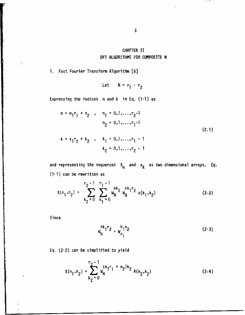
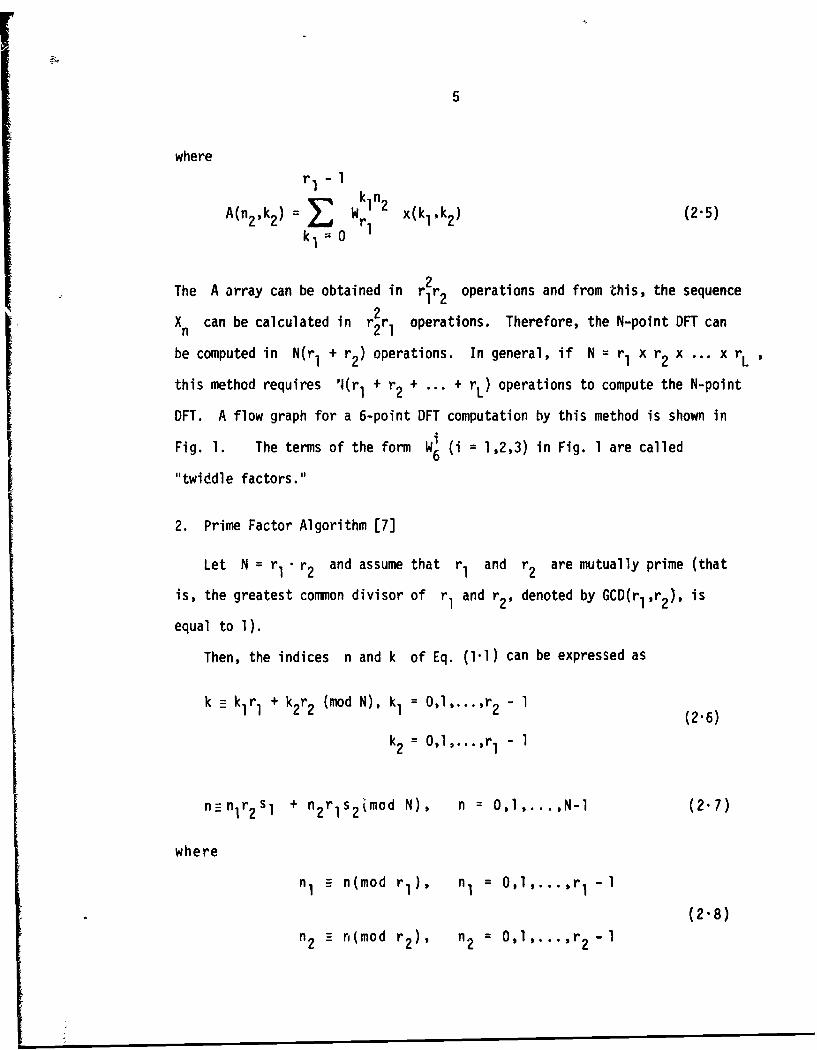
Figure 1. A flow graph of 6-point OFT computation using FFT
X0=x (0 2-point X(010) = x0
x = x(0,2)
x~~l ~2-point X2O
Fiur 2.~l A flown graph) of 6-5n F optto sn F
5
where
A(n2 ,k 2 ) = 1 x(k1,k 2 ) (2.5)
The A array can be obtained in rjr2 operations and from this, the sequence2
Xn can be calculated in r 2r operations. Therefore, the N-point DFT can
be computed in N(r1 + r 2 ) operations. In general, if N = rI x r 2 x ... x rL ,
this method requires '1(rI + r2 + ... + rL) operations to compute the N-point
DFT. A flow graph for a 6-point DFT computation by this method is shown in
Fig. 1. The terms of the form W (i = 1,2,3) in Fig. 1 are called6
"twiddle factors."
2. Prime Factor Algorithm [7]
Let N = rI • r2 and assume that r1 and r2 are mutually prime (that
is, the greatest common divisor of r1 and r2, denoted by GCD(rl,r 2), is
equal to 1).
Then, the indices n and k of Eq. (1-1) can be expressed as
k =- kr1 + k2r 2 (mod N), k1 = O,1,...,r 2 - 1
k= O,l,...,r 1 - l
n:nIr2 Si + n2 r 1 s 2 (mod N), n = 0,1,...,N-1 (2.7)
where
n n(mod rl), n, = 0,1,...,r -r
(2.8)
n 2 - n(mod r 2 ), n2 = ... ,r 1
6
and S,,S2 are solutions of
s r2 1 1 (mod r,)
(2-9)
s 2r, 1 (mod r 2 )
Again, representing the sequences Xk and xn as two dimensional arrays, Eq.
(1.1) can be rewritten as
r, - I r2 -1
X(nl,n 2 ) WN 21 212 x(kl,k 2 )
k2 = 0 k1 = 0
(2.1O)
Since r r 2 kln 1sI rIr 2 k k2 s 1WN WN 2
Eq. (2"10) can be simplified to get
rI- 1k~ nl k2
X(nln 2 ) = Wr A(n2,k2 ) (212)2 k2= 1 l2(-2
wherer -1
A(n2 ,k2 ) Wr2 x(kI ,k2) (2-13)
That is, the N-point DFT can be viewed as r1 r2-point DFT's followed by
r2 rl-point DFT's. If the r, and r2 -point DFT computations require M1 and M2

7
M] M 2operations respectively, the N-point DFT can be obtained in N( 1 +
operations.
The essential difference between the PFA and the FFT are the following:
a. The factors of N must be mutually prime in the PFA
b. There are no twiddle factors in the PFA
c. The index mapping which converts the one-dimensional arrays in Eq. (11)
into two-dimensional (in general, multidimensional) arrays is different
for the two cases.
Fig. 2 depicts the computation of a 6-point DFT using the PFA.
3. Nested Algorithm [3]
The DFT relation in Eq. (1l1) can oe represented in the matrix form
X Wx (2.14)
where
0 0
X x1
X xlX =: , x
XN - LXN - 1
and W is the N-point DFT matrix, the (i,j)th element of which is equal to Wij
LetN = r 1r 2
8
GCD (rI,r 2 ) = 1
W= r - point DFT matrix
W2 r2 - point DFT matrix
Then, Eq, (2.14) can be rewritten as
X = Pout (W1 * W2) Pin (2.15)
where P out and Pin are two NxN permutation matrices, and * denotes themin
"Kronecker product" operation.
Furthermore, let _X = P-out X and x = P x . (2'16)a I
Then Eq. (2 15), in terms of X and x , becomes
X = (W1 * W2 ). x (2.17)
It is possible to decompose W as
W = SCT (2.18)
where
T = M x N incidence matrix (that is, a matrix which has
its elements taking values -1, 0 or 1 only)
C = M x M diagonal matrix
S = N x M incidence matrix
9
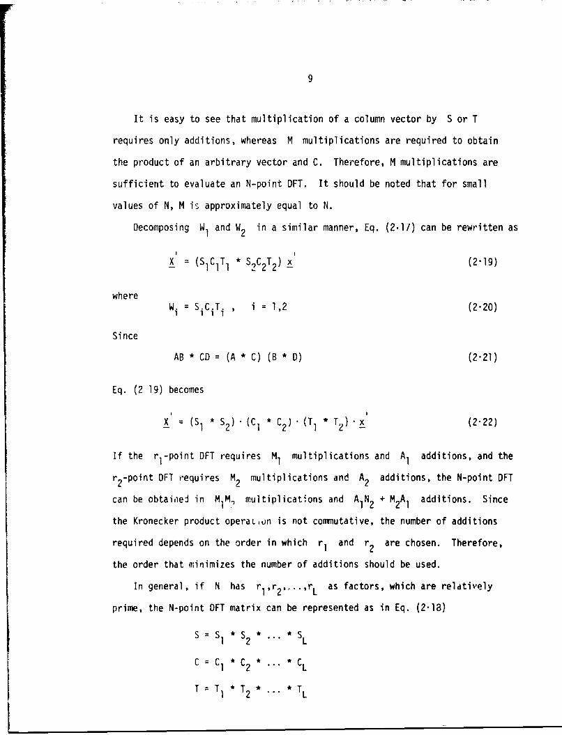
It is easy to see that multiplication of a column vector by S or T
requires only additions, whereas M multiplications are required to obtain
the product of an arbitrary vector and C. Therefore, M multiplications are
sufficient to evaluate an N-point DFT. It should be noted that for small
values of N, M is approximately equal to N.
Decomposing W1 and W2 in a similar manner, Eq. (2.11) can be rewritten as
(SIC1 T1 * $2 C2T2 ) T (2-19)
whereWi = SiC.T. , i = 1,2 (2.20)
Since
AB * CD = (A * C) (B * D) (2"21)
Eq. (2 19) becomesI I
X = * $ S (C' * C2 ) (T1 * T2) x (2-22)
If the rl-point DFT requires M, multiplications and A1 additions, and the
r 2 -point DFT requires M. multiplications and A2 additions, the N-point DFT
can be obtainei in M1 M multiplications and AIN 2 + M2 Al additions. Since
the Kronecker product operaLun is not commutative, the number of additions
required depends on the order in which rI and r 2 are chosen. Therefore,
the order that minimizes the number of additions should be used.
In general, if N has rl,r 2,..., rL as factors, which are reldtively
prime, the N-point DFT matrix can be represented as in Eq. (2.18)
SSl * 2* ... SL
C=C *C * ... L
T T 1 T2 * L
10
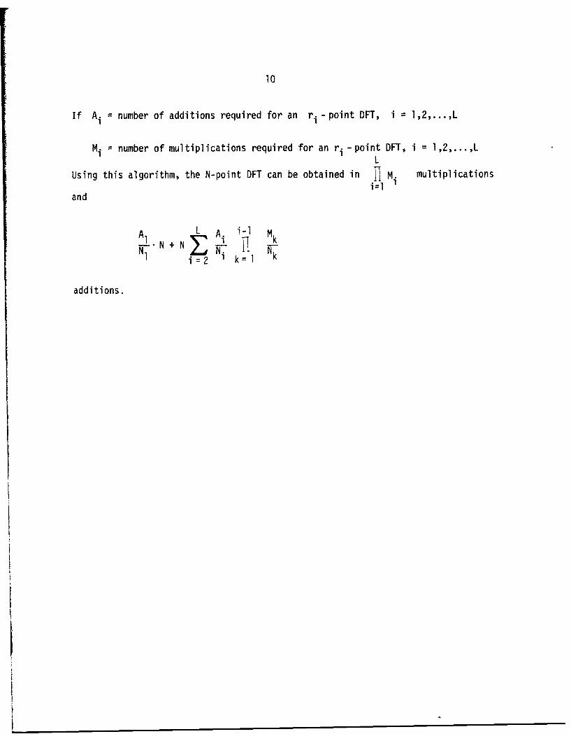
If A. : number of additions required for an ri -point DFT, i = 1,2,...,L
Mi = number of multiplications required for an ri -point DFT, i = 1,2,...,LL
Using this algorithm, the N-point DFT can be obtained in i M, multiplicationsi=l
and
A1 L Ai i-l MkllN +N L i Nki=2 k= k
additions.
11
CHAPTER III
SHORT LENGTH DFT ALGORITHMS
The central idea behind deriving efficient algorithms for computing the
DFT of short length sequences is to reduce the problem to one of evaluating
cyclic convolutions. It was shown by Rader [8] that if N is a prime, the
N-point DFT can be viewed as an (N-l)-pcint circula•r convolution. When N
is a prime power (i.e., N = p r, p 2), the N-point DFT can be obtained by
computing a (P-l).pr-l point convolution and two pr-l point convolutions [9].
Efficient algorithms exist for performing circular convolution. These can
in turn be employed to compute the DFT, after replacing it with a convolution
problem. In order to derive these algorithms it is best to employ polynomial
multiplication techniques. To this end, consider the problem of obtaining
the circular convolution of two sequences a, n = 0,1,...,N-1 and bn,
n = O,l,...,N-l, defined by
N-1
c n akbn-k , n = O,1,...,N-1 (3.1)
k=O
where the indices are evaluated modulo N. Eq. (3"1) can be viewed as a poly-
nomial multiplication problem. That is, if
N-1
p(x) = 2 aiXi
i=O
N-1
q(x) = biXi
i=O
12
and N-Iy(x) = =0Cx
then
y(x) = p(x; q(x) mod (xN 1) (3.2)
For small values of N, the coefficients of the polynomial y(x) can be com-
puted efficiently as explained below:
k
Let T(x) = xN -_ = T Ti(x) be the decomposition of T(x) into itsi=l
irreducibles. By the Chinese Remainder Theorem, the coefficients of r(x)
can be obtained from those of ri(x) = p(x). q(x) mod Ti(x), i = 1,2,... ,k.
It is shown in [10] that the minimum number of multiplications needed to
compute the coefficients of r(x) in this way is 2N-k. When N is small,
it is possible to achieve this minimum, but for large values of N , the
number of additions required will be very large and this method becomes
inefficient.
Algorithms for finding the DFT of short sequences have been derived and
are given in [3] and [4], Efficient algorithms for 11 and 13-point DFT's
are presented here. A more efficient algorithm for 9-point DFT than those
in [3] and [4] is also presented. Other known short transforms [3] are also
listed.
I
13
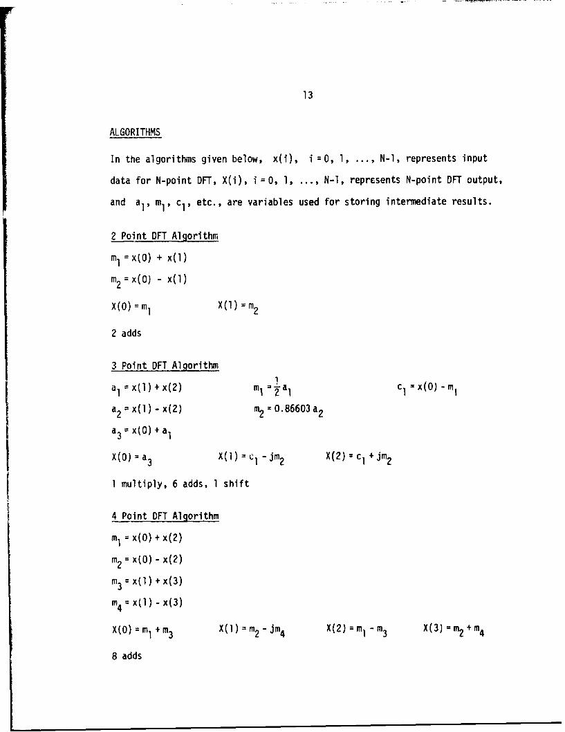
ALGORITHMS
In the algorithms given below, x(i), i =0, 1, ... , N-1, represents input
data for N-point DFT, X(i), i=0, 1, ... , N-1, represents N-point DFT output,
and al, mi, cl, etc., are variables used for storing intermediate results.
2 Point OFT Algorithm
mI = x(O) + x(l)
m2 = x(O) - x(l)
X(O) =mI X(1 m2
2 adds
3 Point DFT AlgorithmI
aI = x(l) + x(2) mI =yal cI =x(O) - m1
a2 = x(l)- x(2) m2 = 0.86603 a2
a3= x(O) + aI
X(O)=a 3 X(1)cI -jm 2 X(2) =cl+jm2
I multiply, 6 adds, 1 shift
4 Point DFT Algorithm
mI = x(O) + x(2)
m2 = x(O) - x(2)
mi3= x(l) +x(3)
m = x(l)- x(3)
X(O) =ml +im3 X(l) m2 -jm 4 X(2) =m -im3 X(3) m2 ++m4
8 adds
14
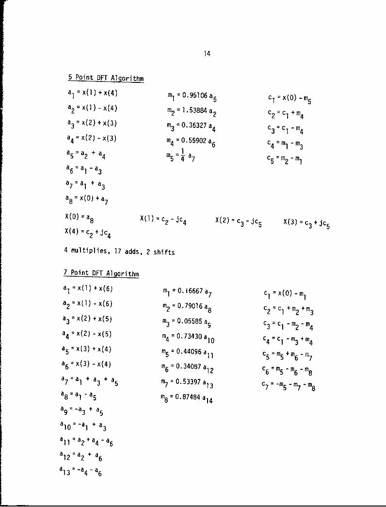
5 Point DFT Algorithm
aI = x() + x(4) m1 = 0.95106 a5 c = x(O) - M5a2 = x(l) - x(4) m2 = 1.53884 a2 c2 = c + M4
a3 = x(2) + x(3) m3 = 0.36327 a4 C3 = C -M4a4 = x(2) - x(3) m4 = 0.55902 a6 c = m -ma 5 a2 + a4 m5=47-a c5 m2-m1
a6 = aI - a3
a7= al + a3
a8 = x(O) + a7
X(O) =a 8 X(1)= c2 - jc 4 X(2) =c3 - jc 5 X(3) = c3 +jc 5
X(4) = c2 +jc 4
4 multiplies, 17 adds, 2 shifts
7 Point DFT Algorithm
a = x(1) + x(6) mI1 = 0. 16667 a7 c = x(O) - Ma2 =x(1) -x(6) m 2 =0. 7 9016a8 c2 =c1 +M2+M3a3 =x(2) + x(5) m3 = 0.05585 a9 c3 = c1 m-2 - m4a4 = x(2) - x(5) m4 = 0.73430 a 10 c4 = C 4 m-3 +M 4a5 = x(3) + x(4) m5 = 0.44096 a11 c5 = m5 +M6 -n'7a6 = x(3) - x(4) m6 = 0.34087 a12 c6 = m5 m-6 m-8a7 =al + a3 + a5 m7 =0.53397a13 c7 =-m5 -m7 -m8
a8 = a , " a5 m8 = 0. 8 7484 a, 4
a9 =-a 3 + a5
al 0 = -al + a3
a11 =a2 +a4 -a 6
a12 =a 2 + a6
a1 3 =-a 4 - a6
15
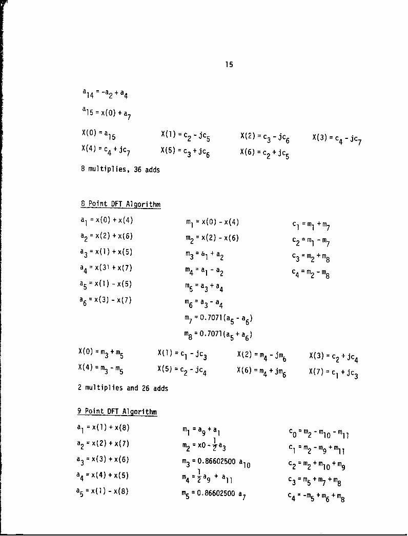
a14 -a2 + a4
a15 x(O) +a 7
X(O) = a15 X(l)= c 2 -jc 5 X(2) c3 - jc 6 X(3) = c4 jc7X(4) = c4 +jc 7 X(5) c3 +jc 6 X(6) = c2 +jc 5
8 multiplies, 36 adds
8 Point DFT Algorithm
a, = x(O) +x(4) ml = x(O) - x(4) cI = mI +m7
a2 = x(2) + x(6) m2 = x(2) - x(6) c2 = ml _ m7
a3 =x(l)+x(5) m3 =al+a2 c3:m2+M8
a4 :x(3) +x(7) m4 :a, -a2 c4 m2 m8
a5 = x(1)- x(5) m5n = a3 + a4
a6 = x(3)- x(7) m6 = a3 - a4
m7 = 0.7071(a 5 -a 6 )
M8 = 0.7071(a5 +a 6 )
X(O)=m3 +m5 X(l):cl-jc 3 X(2)=m4 -jm 6 X(3)=c 2 +jc 4
X(4) = m3 - m5 X(5)= c2 - jc 4 X(6) = m4 +jm 6 X(7) c I + jc3
2 multiplies and 26 adds
9 Point DFT Algorithm
a,=x(l)+x(8) m1 =a 9 +a+ Ca =m2I -i 0m -Omin
a2 x(2)+x(2) m2 = x0--a 3 c1 =m2 -m9 +m11
a3 = x(3)+x(6) m3 = 0.86602500 a10 c2 =m2 +M10 +M9a4 =x(4)+x(5) m Ia 9 + a c3 m +m7 +8a5 = x(l)- x(8) m5 = 086602500 a7 c4 = _ms +m6 +M8
16
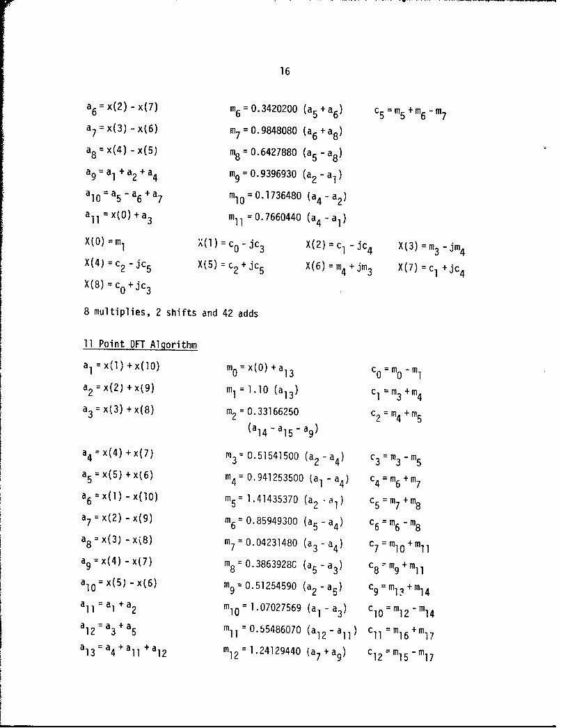
a6 =x(2)-x(7) m6 =0.3420200 (a5+a6) c5 =m5 +m 6-m7
a7 = x(3) -x(6) m7 = 0.9848080 (a6 +a8 )
a8 = x(4) -x(5) m8 =0.6427880 (a5 - a8 )
a9 =a 1 +a 2 +a 4 m9 =0.9396930 (a2 -a 1 )
alo = a5 - a6 +a 7 m lo =0.1736480 (a4 - a2 )
a1 l = x(O) +a 3 m11 = 0.7660440 (a 4 - a,)
X(O)=m1 X(l)=c 0 -jc 3 X(2)=c 1 -jc 4 X(3)=im3 -jnm4
X(4)=c 2 -jc 5 X(5)=c 2 +jc 5 X(6)= m4 +jm 3 X(7)=c 1 +jc 4
X(8) = cO0 +jc 3
8 multiplies, 2 shifts and 42 adds
11 Point DFT Algorithm
a1 =x(1)+x(10) m=x(O)+a 1 3 c0 =m0 -m1a2 =x(2)+x(9) m1 =1.10 (a 13 ) c1 =m3+M4
a3 = x(3) +x(8) m 2 = 0.33166250 c2 = m4 +M 5(a 14 - a1 5 - a9 )
a4 =x(4)+x(7) M 3=0.51541500 (a 2 -a 4) c3=fml3 -m 5
a5 = x(5) +x(6) m4 =0.941253500 (a1 -a 4 ) c 4an 6 +a 6 =x()-x(lO) m 5= 1.41435370 (a2 .l 5=m7+M8
a7 = x(2) - x(9) m 6 = 0.85949300 (a5 - a4 ) c6 = m6 - m8
a8 = x(3) -xý8) m7= 0.04231480 (a 3 - a4 ) c7 = m +M
a9 =x(4)-x(7) m8=0.3863928C (a 5 -a 3 ) c8=m9+Mll
a10 =x(5)-x(6) mi9 =0.51254590 (a 2 -a 5 ) c=m+Ma11 =a +a 2 = 1.07027569 (a1 -a 3 ) c 10 m 12 -m14
a12=a 3 +a 5 mI1 1 = 0.55486070 (a 12 -a 11 ) C11 =ml16 +Ml7
a1 3 =a 4 +a11 +a 12 m12=1.24129440 (a7+a9) c12=mN5-mi 7
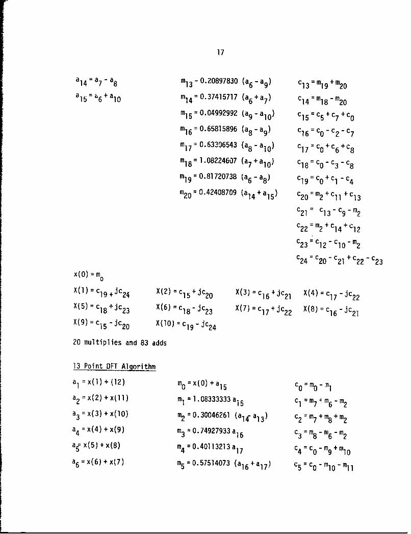
17
a 14 a7 - a8 m13- 0.20897830 (a6 -a 9 ) c132m19 +m20
a15 a +alO m = 0.37415717 (a 6 +a 7 ) c 4 m1 8 -m20
mi5 = 0.04992992 (a 9 - a1 0 ) c1 5 =c 5 +c 7 +c 0
m16 = 0.65815896 (a 8 - a9 ) C161 cO- c 2 -c 7
m17 =0.63306543 (a8 -a 1 0 ) c17 = c 0 +c 6 +c 8
m18 =1.08224607 (a7 +a10 ) C18 =C 0 - c3 - c8
m 19 =0.81720738 (a 6 - a8 ) c19 =c 0 +c1 -c 4
m 20 - 0.42408709 (a 14 +a 15 ) c20 =m2 +C1 1 +c1 3
c2 1 = c1 3 -c9- m 2
c2 2 m2 +C 14 +c 1 2c 23 = C12 -" cO- m 2
c24 c20- c 21 + c22- c23
x(O) =m0
X(1) = c19 +jc 24 X(2) = c1 5 +jc 20 X(3) = c16 +jc 2 1 X(4) = c17 -Jc 2 2
X(5) = c 18 + Jc23 X(6) = c1 8 - Jc 23 X(7) = c17 +jc 22 X(8) = c16 -Jc 2 1
X(9) = c 5 -jc 2 0 X(10) = c-Jc 2 4
20 multiplies and 83 adds
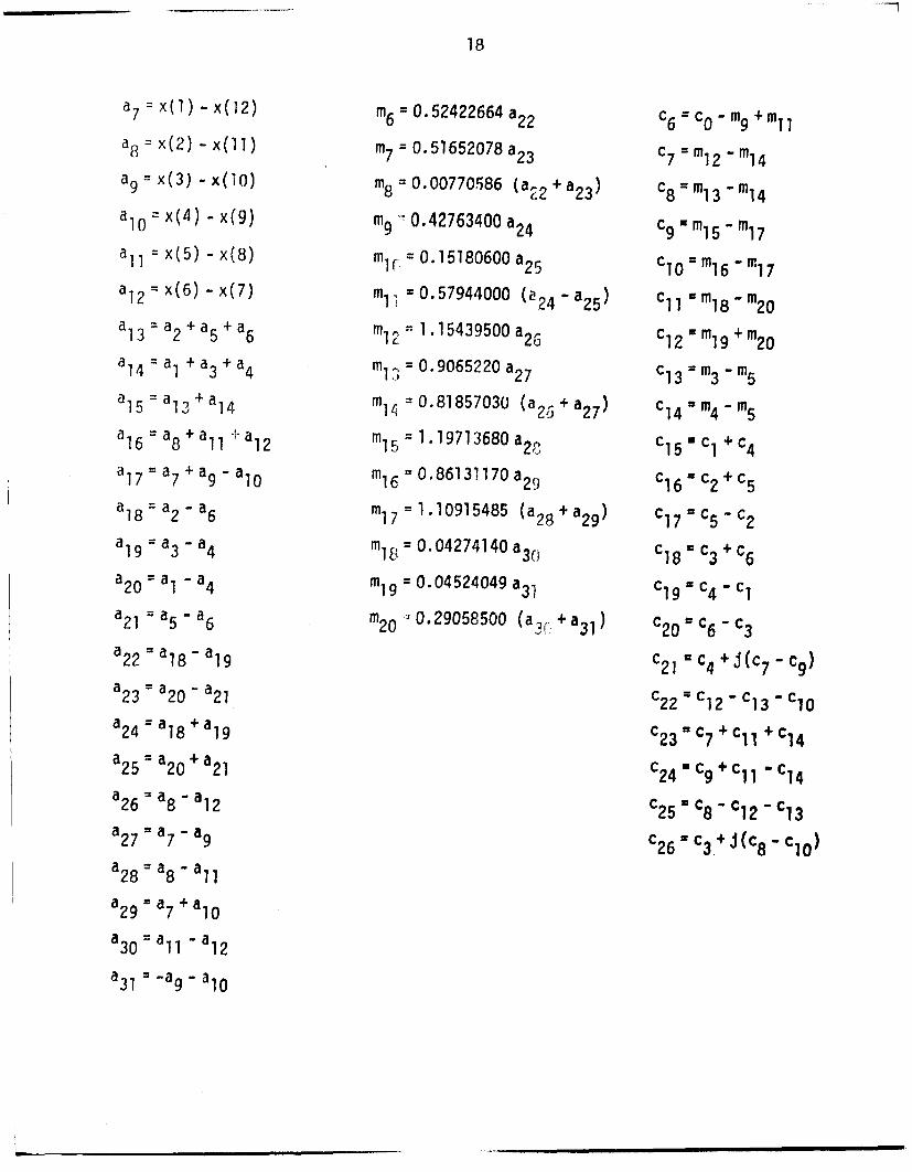
13 Point DFT Algorithm
a1 =x(1)+(12) m0 =x(O)+a 1 5 c0 =mn0 -MI
a2 = x(2) + x(l1) mI 1.08333333 a15 c1 = m7 4 M6 - m-2a3 =x(3)+x(lO) m2 = 0.30046261 (al4-a 1 3 ) c2= m-7 +iM8 + m 2
a4 = x(4)+ x(9) m3 = 0.74927933 a16 c3 = m8 - m6 - m2
a5= x(5) + x(8) m4 = 0.40113213a 7 C4 = c 0 - m9 +m1 O
a6 = x(6) + x(7) m5 = 0.57514073 (a 16 +a 1 7 ) c5 = CO- mlO -mll
18
a7 = x(1)- x(12) m6 = 0.52422664a 2 2 c6 = c0 - m9 +m11
a8 = x(2) - x(1) m7 =0.51652078 a2 3 c7 = m1 2 - m1 4a9 = x(3) -x(iO) m8 =0.00770586 (a2 +a23) c8 m m-in 4
a10 = x(4) -x(9) m9 "0.42763400 a2 4 c9 ,m l 5 -ml7
a,, = x(5) - x(8) mIr = 0.15180600 a2 5 c 10 , m16 - m17
al12 = x(6) -x(7) ml ! 0.57944000 (a 2 4 -a 2 5 ) c11 ," 18 -m2 0
a 3 = a2 +a 5 +a 6 ml = 1 . 5439500 a2 C 2 =m +Ma = a +a+a4 m =0.9065220 a2 7 C2 m3"ma14 a1 + 3 +4 27 13 m3 -i 5
al 5 =al 3 +1 a 4 m1 0.81857030 (a2+a27) c 1 4 =m 4 .i 5
8 11 +a12 mI =1. 19713680a 20 15 C1+C4a16 a +a -a C +C7 a7 9 - 0 m16 ' 86131170a 2 9 16 2 5a18 = a2 - a6 ml17 = 1.10915485 (a 2 8 +a 2 9 ) c1 7 c5 -c2
a19 = a3 - a4 mit; = 0.04274140 a3 0 c18, c3 + 6
a20 = aI - a4 m19 = 0.04524049 a3 . c19= c4. c1a21 =a -a 6 m2 0 0.29058500 (a,, +a3 1 ) c 2 0 "c6 -c 3
a2 2 = a18 - a19 c2 1 ' c4 +R(c 7 - cg)
a2 3 = a 2 0 - a2 1 C2 2 ' c 1 2 - c 1 3 - c 1 0
a24 = a18 +a 19 c2 3 c7 +Cli +C1 4
a25 = a20 + 21 c24 = c9 + C11 "14
a26 = a8 - a12 c2 5 c8- c12- c1382 7 =a 7 -a 9 c2 6 ' c 3 + j(c 8 - c1 0 )
a2 8 a78 - aa28 :as" 11
a29 a 7 +a 10
a30 a 11 a812
a31 -a9 -10
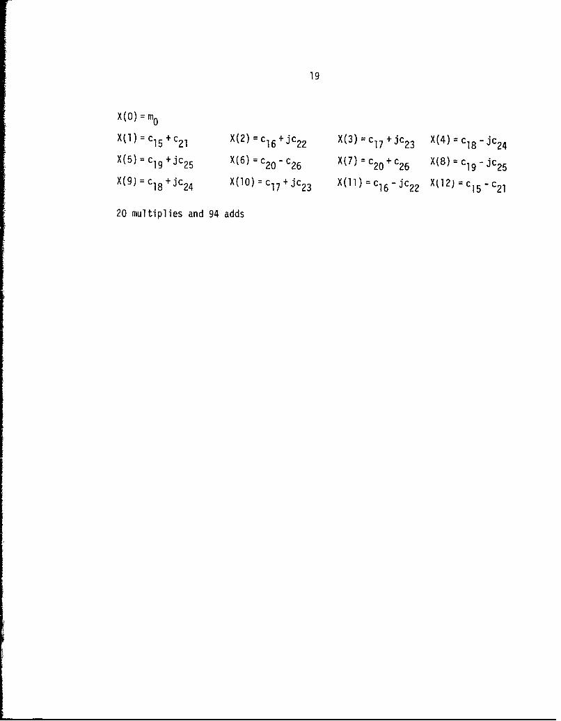
19
X(O) =m0
SX(1) = c 15 +c 2 1 X(2) = c16 +jc 22 X(3) = c 17 +jc 23 X(4) = c18 - jc 2 4
X(5) = c 19 +Jc25 X(6) = c20 -c26 X(7) = c20 +c 26 X(8) = c19 -Jc 2 5X(9) = c18 +jc 24 X(1O) = c1 7 +jc 2 3 X(1)= c16 - jc 22 X(12) = c15 -c 2 1
20 multiplies and 94 adds
20
CHAPTER IV
FIXED POINT PFA AND WFTA ERROR ANALYSIS
The DFT algorithms are often implemented by special purpose digital hard-
ware using fixed point arithmetic. Accuracy requirement is one of the impor-
tant factors which influences the decision about the word size of such implemen-
tations. Therefore, it is desirable to estimate the roundoff noise generated
in the DFT computation. The effrect of fixed point arithmetic on the roundoff
noise in FFT computations has been studied in [11] and [12]. An estimate of
the roundoff noise in the case of the PFA and the WFTA is obtained here using
a statistical model.
Addition and multiplication by constants are the only two arithmetic
operations needed to implkment the DFT algorithms. If the input data is
properly scaled to avoid overflow during additions, no error will be introduced
in the DFT output due to addition operations. However, when two fixed point
numbers are multiplied, the result has to be rounded. This introduces roundoff
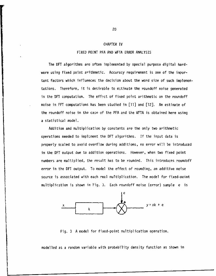
error in the DFT output. To model the effect of rounding, an additive noise
source is associated with each real multiplication. The model for fixed-point
multiplication is shown in Fig. 3. Each roundoff noise (error) sample e is
xy y=xk + e
Fig. 3 A model for fixed-point multiplication operation.
modelled as a random variable with probability density function as shown in
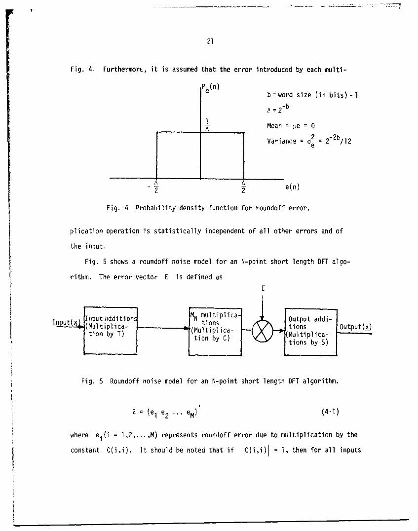
21
Fig. 4. Furthermore, it is assumed that the error introduced by each multi-
Pe(n)e b=word size (in bits)-1
=
-4" 1A Mean = e :0
Variance = 2= 2-2/2
-2 e(n)
Fig. 4 Probability density function for roundoff error.
plication operation is statistically independent of all other errors and of
the input,
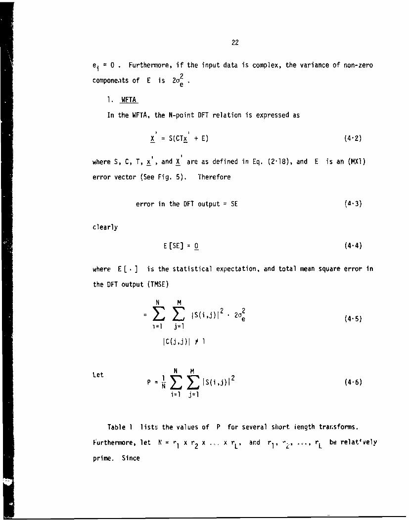
Fig. 5 shows a roundoff noise model for an N-point short length DFT algo-
rithm. The error vector E is defined as
E
S~MN multiplica-ut( nput Additions N tions Output addi-
Inu (Multiplica- __ (Multiplica- tions Output(x)
tion by T) tion by C) (Multitipliction~ton by C)(uli )ia
Fig. 5 Roundoff noise model for an N-point short length DFT algorithm.
E (e e2 ... eM) (4.1)
where ei(i = 1,2,...,M) represents roundoff error due to multiplication by the
constant C(i,i). It should be noted that if jC(i,i)l 1, then for all inputs
22
ei = 0 . Furthermore, if the input data is complex, the variance of non-zero
componeots of E is 2a2e
1. WFTA
In the WFTA, the N-point DFT relation is expressed as
X. = S(CTx + E) (4"2)
where S, C, T, x , and X' are as defined in Eq. (2"18), and E is an (MXI)
error vector (See Fig. 5). Therefore
error in the DFT output = SE (4.3)
clearly
E [SE] = 0 (4.4)
where El ] is the statistical expectation, and total mean square error in
the DFT output (TMSE)
N M
- 'i~~l 2 202( -5
1=1 j=l
IC(Jj)I ý 1
Let N M
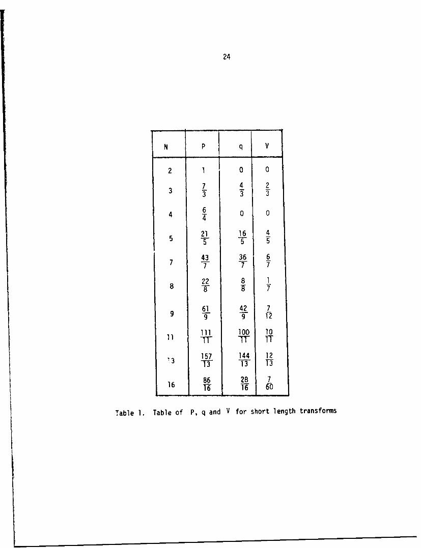
P = 12 E lS(i,j)I 2 (4-6)i=l j=l
Table I list', the values of P for several short iength trarnsforms.
Furthermore, let N =I x r 2 x ._ x rLt ard r >, ... , L be relat'vely
prime. Since
23
S = Sl * S2 *...* SL (4"7)
it follows that
N M"E "E IS(ij)12 = N P1 P2 ... PL (4.8)
i~l j=1
where Pi is as defined in Eq. (4.6) for N = r. For all values of 11, it
can be verified that
C(ll) = 1 (4'9)
and S(i,l) = 1, i - 1,2,...,N (4'10)
Using Eqs. (4 8) (4 10), it can be shown that22 P I P2 -' P L
TMSE < 2 N2 a 2 N - I) (4.11)
or, equivalently,
TMSE < 2 K1 N2 2 (4212)I e ( '2
where
K 1 2 -L 1 (4.13)N
It is interesting to note that the roundoff noise does not depend on the
order in which short length transforms are combined to obtain longer length
transforms.
24
N P q V
2 1 0 0
37 4 23 3 3
4 0 04
21 16 4
7 43 36 67 T 7
8 22 8 1T 9 7
61 42 7T i-2
111 100 10
157 144 12",3 f 1--3- T 3
86 28 716 T 6 16 6-0
Table 1. Table of P, q and V for short length transforms
25
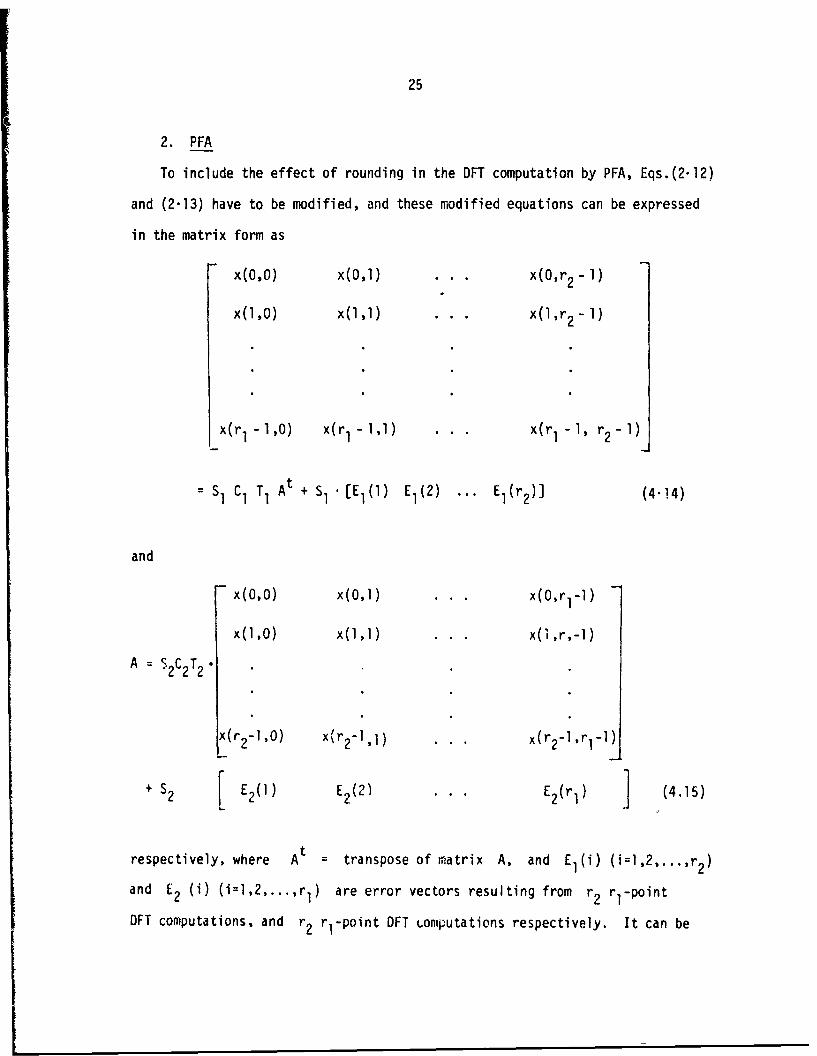
2. PFA
To include the effect of rounding in the DFT computation by PFA, Eqs.(2.12)
and (2.13) have to be modified, and these modified equations can be expressed
in the matrix form as
x(0,O) x(Ol) . . . x(O,r 2 -1)
x(l,O) x(l,l) . . x(l,r 2 -1)
x(r 1 -1,0) x(r-1 -,l) . . . x(r -I , r 2 -I)
SI C1 T1 At + Sl'[El(1) E1 (2) ... El(r 2 )] (4.14)
and
x(0,O) x(0,1) . . . x(O,r 1-1)
x(1,0) x(1,1) .x(i ,r,-1)
A = $2 C2 T2 •
x(r 2 -1,0) x(r 2-",1) . . . x(r 2-1,r 1-1)
+ S2 E2 (l) E2 (2) . . E2 (rl) (4.15)
trespectively, where A transpose of matrix A, and El(i) (i=1,2,...,r 2 )
and E2 (i) (i1,2,.. .,r) are error vectors resulting from r 2 ri-point
OFT computations, and r 2 r,-point OFT Lomputations respectively. It can be
26
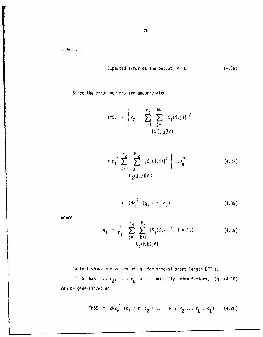
shown that
Expected error at the output = 0 (4.16)
Since the error vectors are uncorrelated,
rl M1
TMSE jr2 11 , jSl(ij)j 2
i=l j=l
+ r 2 1S2(i.)I 2 .2 (4.17)i =l j=l
r2(j ")I•
2Nae2 (ql + rl q (4.18)e (q 2)
whereSr. M. 21 .2
q i E t. ISi(J,k)j, i = 1,2 (4.19)j=1 k~l
ýl(k,k)I#l
Table 1 shows the values of q for several short length DFT's.
If N has rl, r 2, ... , rL as L mutually prime factors, Eq. (4.18)
can be generalized as
TMSE = 2No 2 (q, + r, q + rlr r (4.20)
Oe 2 + 2 L- qL•
27
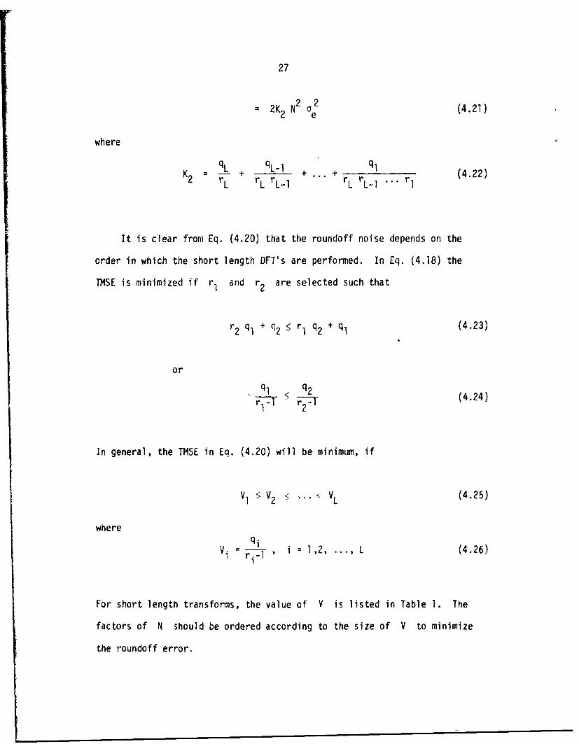
= 2K2 N2 G2 (4.21)2 e
where
K __ q l*
2 rL + rL-l + + r (4.22)K2 rL rL rL-l r L rL-1 - r1
It is clear from Eq. (4.20) that the roundoff noise depends on the
order in which the short length DFT's are performed. In Eq. (4.18) the
TMSE is minimized if rI and r2 are selected such that
r 2 q, + q2 1r q2 + ql (4.23)
orq, q q2q1 < q (4.24)1 2
In general, the TMSE in Eq. (4.20) will be minimum, if
VI ý V2 < *... VL (4.25)
where
qiVi ri.1 ,i:1,2, ..... , L (4.26)
For short length transforms, the value of V is listed in Table 1. The
factors of N should be ordered according to the size of V to minimize
the roundoff error.
28
Similar results are obtained in [12] for the FFT case and are given below:
Expected error in the output = 0 (4.27)
and
TMSE (2 N + 2 4 (4.28)
where N is the transform size. For large values of N
TMSE 2 k3 N2 (where k3 = 1) (4.29)
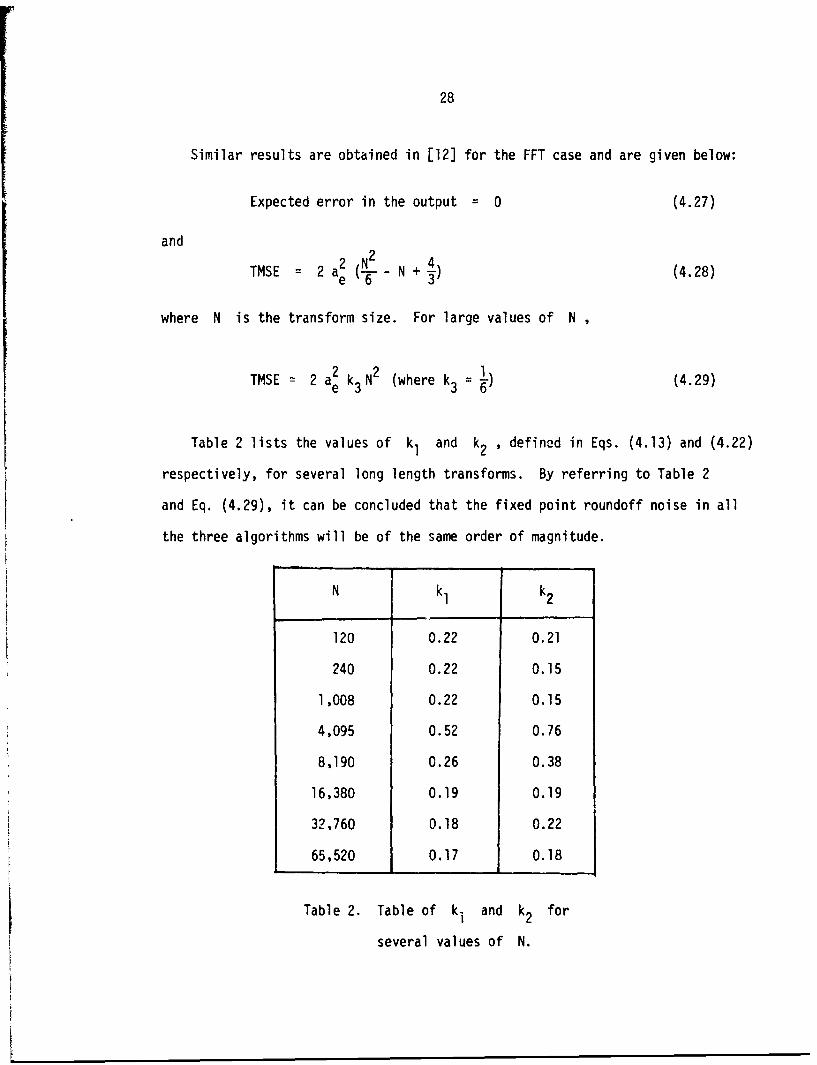
Table 2 lists the values of k1 and k2 , defined in Eqs. (4.13) and (4.22)
respectively, for several long length transforms. By referring to Table 2
and Eq. (4.29), it can be concluded that the fixed point roundoff noise in all
the three algorithms will be of the same order of magnitude.
N kI1 k 2
120 0.22 0.21
240 0.22 0.15
1,008 0.22 0.15
4,095 0.52 0.76
8,190 0.26 0.38
16,380 0.19 0.19
32,760 0.18 0.22
65,520 0.17 0.18
Table 2. Table of ki and k2 for
several values of N.
29
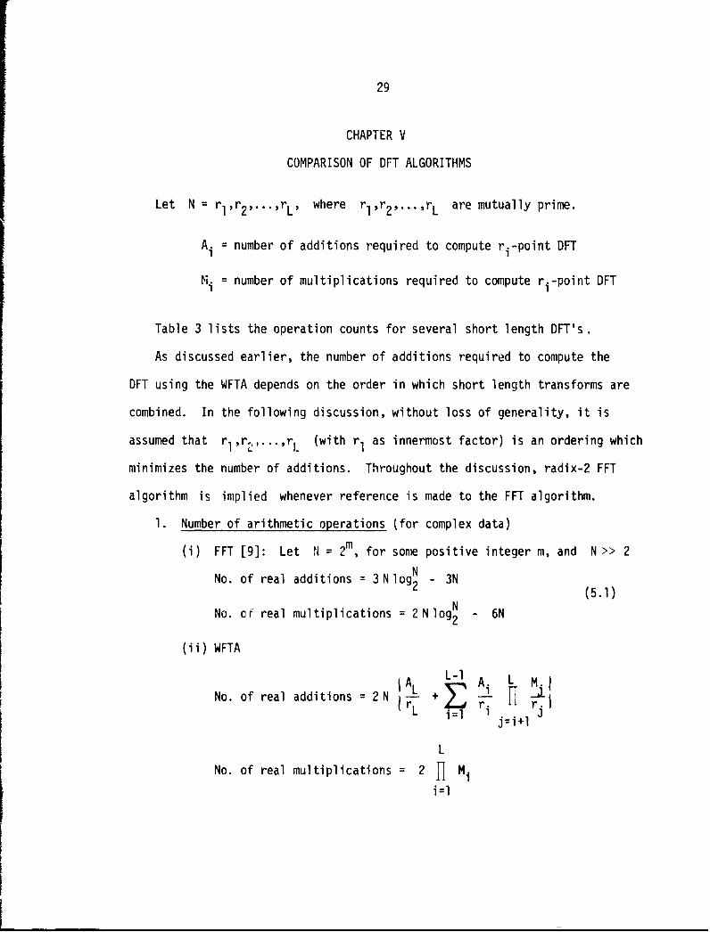
CHAPTER V
COMPARISON OF OFT ALGORITHMS
Let N = rl,r 2 , ... ,rL, where rl,r 2 ,...,rL are mutually prime.
Ai = number of additions required to compute ri-point DFT
Mi = number of multiplications required to compute ri-point DFT
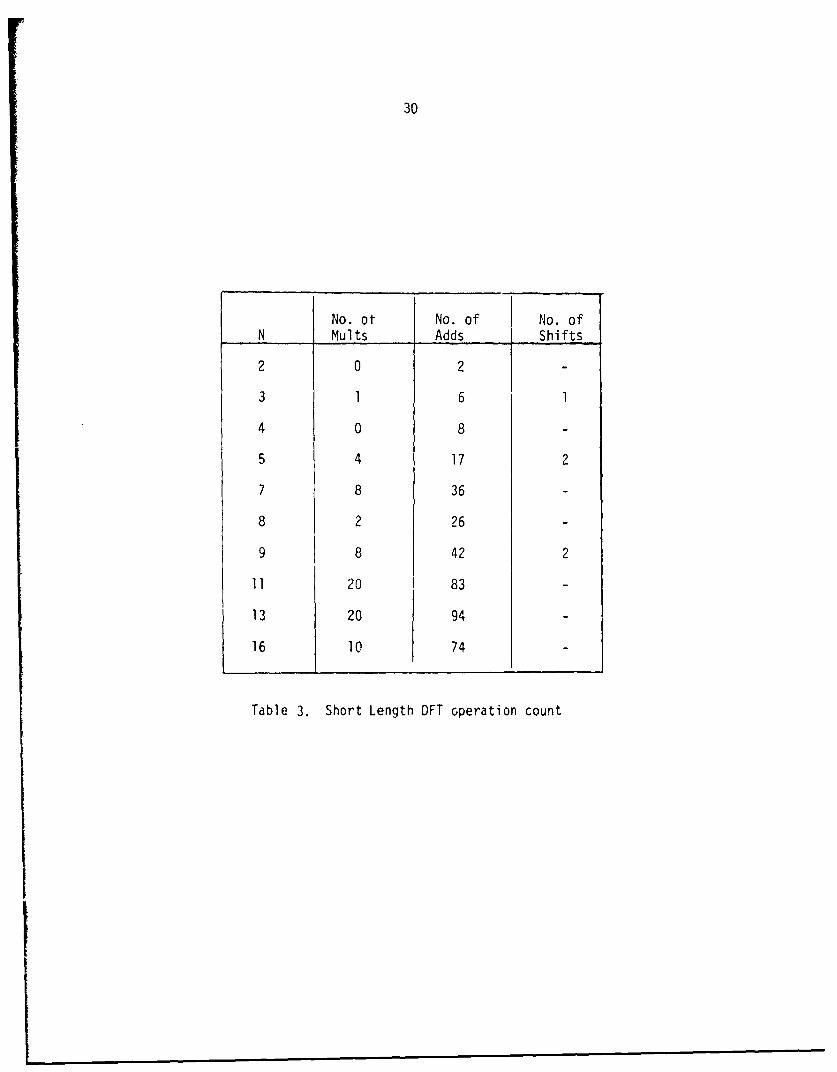
Table 3 lists the operation counts for several short length DFT's.
As discussed earlier, the number of additions required to compute the
DFT using the WFTA depends on the order in which short length transforms are
combined. In the following discussion, without loss of generality, it is
assumed that rl,r...,r. (with rI as innermost factor) is an ordering which
minimizes the number of additions. Throughout the discussion, radix-2 FFT
algorithm is implied whenever reference is made to the FFT algorithm.
1. Number of arithmetic operations (for complex data)
(i) FFT [9]: Let N = 2m, for some positive integer m, and N>> 2
No. of real additions = 3NlogN - 3N2 N (5.1)
No. o( real multiplications = 2 Nlog• - 6N
(ii) WFTA
ýA LL i=L-1 i A I M.)rj
No. of real additions = 2 N + -It
L
No. of real multiplications = 2 FjMi
i=l
30
No. ot No. of No. ofN Mults Adds Shifts
2 0 2
3 1 6 1
4 0 8 -
5 4 17 2
7 8 36 -
8 2 26 -
9 8 42 2
11 20 83 -
13 20 94 -
16 10 74 -
Table 3. Short Length DFT operation count
31
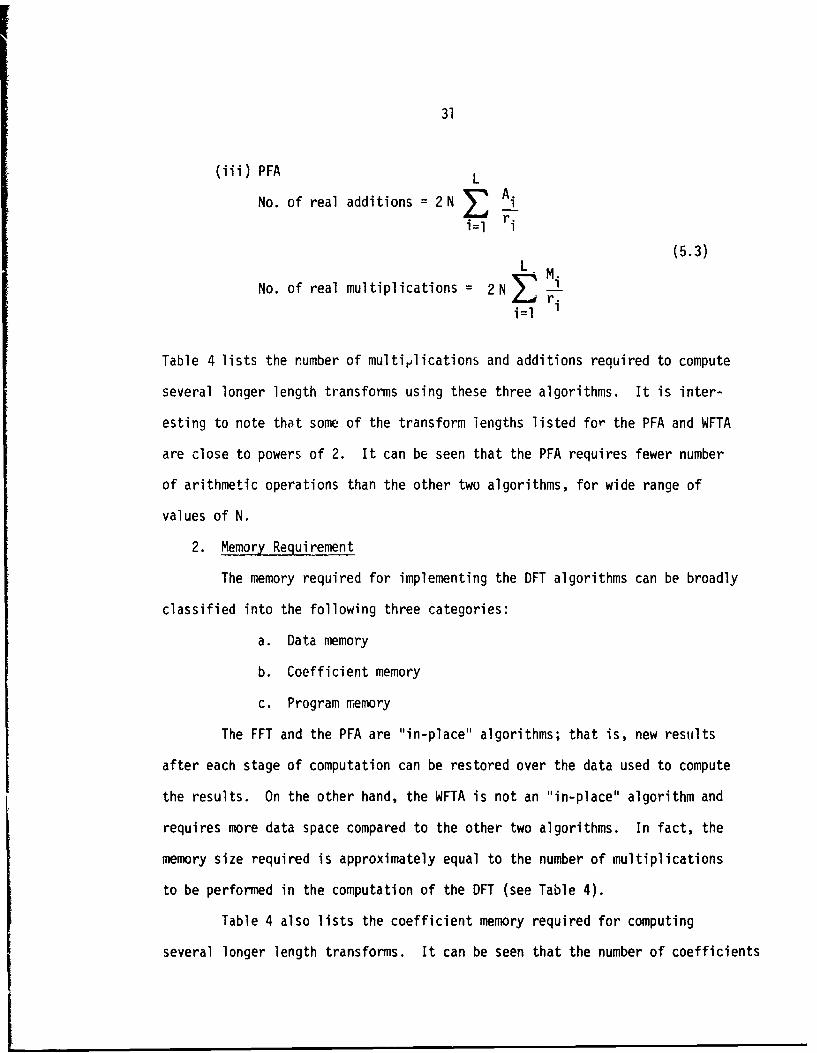
(iii) PFA L
No. of real additions = 2 N Aii~ r.
(5.3)
No. of real multiplications = 2N r
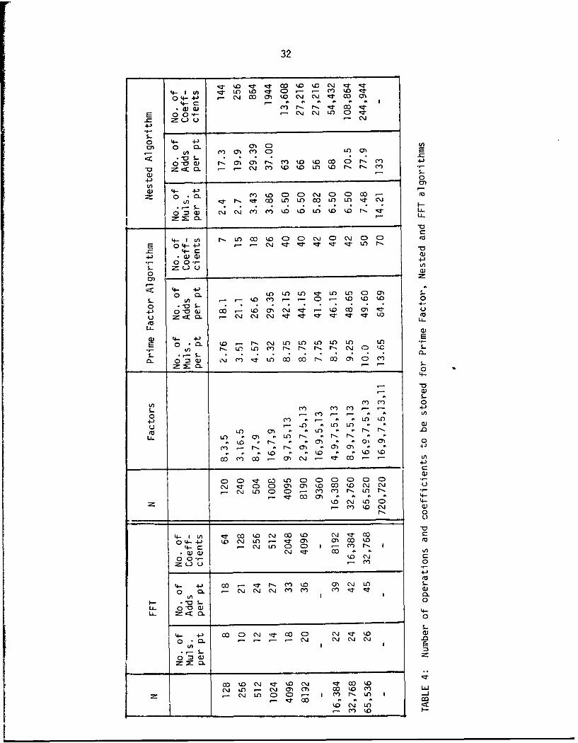
Table 4 lists the number of multiilications and additions required to compute
several longer length transforms using these three algorithms. It is inter-
esting to note that some of the transform lengths listed for the PFA and WFTA
are close to powers of 2. It can be seen that the PFA requires fewer number
of arithmetic operations than the other two algorithms, for wide range of
values of N.
2. Memory Requirement
The memory required for implementing the DFT algorithms can be broadly
classified into the following three categories:
a. Data memory
b. Coefficient memory
c. Program memory
The FFT and the PFA are "in-place" algorithms; that is, new results
after each stage of computation can be restored over the data used to compute
the results. On the other hand, the WFTA is not an "in-place" algorithm and
requires more data space compared to the other two algorithms. In fact, the
memory size required is approximately equal to the number of multiplications
to be performed in the computation of the DFT (see Table 4).
Table 4 also lists the coefficient memory required for computing
several longer length transforms. It can be seen that the number of coefficients
32
0 41- cm CM MO 0)U C Mo O
4-'
0 4-- 4-)
-) 0 C 0) C) C)f 0
a)O r, (n0 N.. Cr) 10 U) COOC r-. Mr 4-CL - - M km tDU U-) LO r. P. Cr)
4-) 0)
(D 4- +-'m tD0 C),U 0CD M0CDC 0C0
2= 0 r . -I N t 00 CO LO 00 CO U O U) C\JS-I
o0m 0 CMj CM Cr) C') U)ý U U; U) U) P. Uj L.
4-__ V)V f 0 'O C D ClC \ : :
4- C
4- 0-4' -a) d) (DtU) N
0 0.- 4-.'
0Y)
< 4- 4-)0 0. UC) UO UO LO LO U) 00
S- L) - - U) Mr ,- -0D- ID ko U) 00 .- a S- 4-
4)~ 0-0 C - U 0; Jlý ar-U)ll C6O cl .Z.u
u 2 < C - CMicMiCMj It .J-- -T U)T i
0) 4- 4-EE 0 .0. U) r, CJ LO U') UO LO U-) Ul)
S- r*r-Sr C 9 k
a- 0 -3 (D 4'i m :I OC
4-
-0
aS-.
tn C') c') 0
0 - r - - - t
u p 1 n U) U); a a a)
ito U) 0) a U ~ . C..f
Li. U) . 0) a ) . r-. %. .
a ) * r- a ý a ) 01 m 0
4-'
_____ Cý o ýCýL 4-)
0) 0 q C)LOC CU ) 00000 0-d-~ 00 0 C) CO UCM CM M ou
C -Lo CO 0) a M a atzr 0M m) .0 4-
k.0 r U) CD 0
*0
4-1lu) -tCO- 0 ) CMo Ci oU CMj -z CO0 4--4-> q.0 CMJ U) - <,0), m CO U)
4-C a CMj U) 00 C3 - CrMNa0) a) CM j CO a aVS)
00-- )C C:
:zu) u -C,0
S-4-'
0A 0< CL CM C4M-r r C,~
0
S-
0-0 - - .- .- CMi CMi CM CM
0V)
-CM U) 0 0C)- I CY)r, N. ) I -
to cl CO a<U) CM U
33
to be stored is significantly less for the PFA compared to the other two
algorithms. The sine-cosine values required in the FFT method can be computed
recursively as needed; thus savings in memory space can be achieved. The
disadvantage of such a scheme is that the computation time is increased by
about 15%. Similar savings in the memory requirements can be achieved in the
case of the WFTA. However, such implementations could be very inefficient in
terms of speed.
Of the three DFT algorithms being considered, the FFT program requires
minimum space. Besides this, input and output re-ordering is very systematic
for the FFT, where as they are less so and may require storage in the case of
the other two algorithms. The computation of the re-ordering vectors as they
are needed saves storage, but is less efficient. However, by using a different
input-output re-ordering scheme and adding a small amount of extra hardware,
in the case of special purpose hardware implementations, this storage space
can be saved. This is discussed further in Chapter VI.
3. Programming Complexity
Programming of the FFT is ifuch simpler compared to the other two algorithms.
This is mainly because of the complicated indexing scheme to be used in the
PFA and the WFTA. To illustrate this, a FORTRAN program for 120-point PFA is
listed in the Appendix. This can be compared with the FFT programs given in
[1]. It should be noted that the WFTA is not an inplace algorithm. This
further complicates Lhe programming of WFTA.
4. Effect of finite word-length arithmetic
The use of finite precision arithmetic in the DFT computation introduces
error in the output. The effects of finite register length in FFT calculations
is discussed in [1, 5, 11, 12]. Because of the complicated structure of the
34
PFA and the WFTA, it is difficult to analyze the effects in these algorithms.
The PFA and WFTA require fewer arithmetic operations compared to the FFT.
It is very likely that the floating-point DFT computation by these methods will
introduce smaller error than in the case of the FFT. By computing the coeffi-
cients needed using higher precision arithmetic, the effects of coefficient
quantization can be reduced in all the methods. The effects of fixed point
arithmetic in DFT computation was discussed in Chapter IV.
35
CHAPTER VI
A HARDWARE IMPLEMENTATION OF PRIME FACTOR ALGORITHM
It is often necessary to build special purpose hardware for computing
the discrete Fourier tra;isform. With the availability of low cost micropro-
cessors, it is now economical to conceive of processor-based hardware struc-
ture. The WFTA is not suitable for this purpose if transforms of long
sequences are required. In such cases, a choice has to be made between the
FFT and the PFA. Multiplication is one of the slcwer arithmetic operations
in processor-based systems. The ratio of multiply to add times could be as
large as 10 to 15. Therefore, from the earlier discussion it is eviderit
that the PFA is better suited for this purpose than the FFT. Furthermore,
there are certain other advantages in using the PFA for hardware implementa-
tion, and this will be made clear soon.
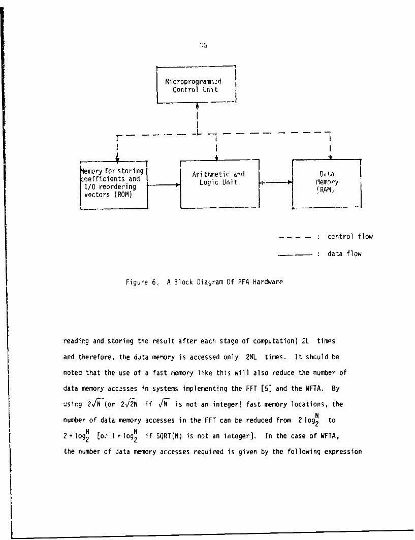
A simple block diagram of PFA hardware is as shown in Fig. 6. The dia-
gram is self-exDlanatory. The coefficients are stored in the read only
memory (ROM). The initial and final reordering vectors are also stored in
the ROM. The DFT algorithm is implemenced at the microprogram level to
increase the speed of the system. The input-output section is not shown
in the diagram.
This system can be speeded up further by adding a few inexpernsive hardware
blocks to it. By providing a small number of high speed storage registers
(a maximum of 64 words is sufficient for N as large as 720,720) it is pos-
sible to reducc the number, of accesses to the data memory. The intermediate
results during computation of short length DFT's can be stoted in this fast
memory. If N has L factors, then each data point is accessed (for
Mi croprograniT,-aiControl Unit
r -I I I
4emory for storing Arithmetic and Dutacoefficients andLogic Unit riemory1/0 reordering Logic Uni P0Memor
vectors (ROM) j '
ccrtrol flow
data flow
Figure 6. A Block Diagram Of PFA Hardware
readirn and storing the result after each stage of computation) 2L times
and therefore, the dita memory is accessed only 2NL times. It shculd be
noted that the use of a fast memory like this will also reduce the number of
data memory accasses 4n systems implementing the FFT [5] and the WFTA. By
usirg 2A-(or 2V2N if F/N is not an integer) fast memory locations, the
number of data memory accesses in the FFT can be reduced from 2 log2 to
N N
2+ log2 Co.- 1 +109 2 if SQRT(N) is not an integer]. In the case of WFTA,
the number of data memory accesses required is given by the following expression
37
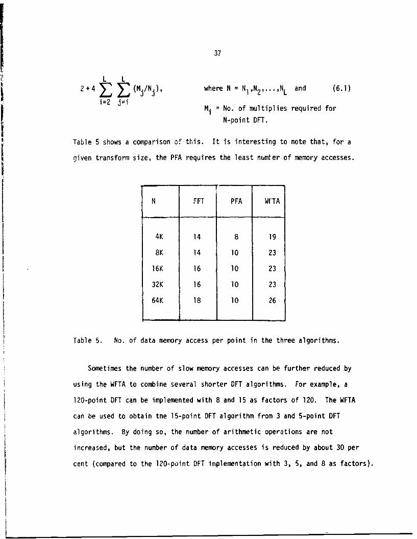
2+4 • (M /N1 ), where N = Nl,N 2 ,...,NL and (6.1)
i=2 Mi = No. of multiplies required for
N-point DFT.
Table 5 shows a comparison of this. It is interesting to note that, for a
given transform size, the PFA requires the least numler of memory accesses.
N FFT PFA WFTA
4K 14 8 19
8K 14 10 23
16K 16 10 23
32K 16 10 23
64K 18 10 26
Table 5. No. of data memory access per point in the three algorithms.
Sometimes the number of slow memory accesses can be further reduced by
using the WFTA to combine several shorter DFT algorithms. For example, a
120-point DFT can be implemented with 8 and 15 as factors of 120. The WFTA
can be used to obtain tne 15-point DFT algorithm from 3 and 5-point DFT
algorithms. By doing so, the number of arithmetic operations are not
increased, but the number of data memory accesses is reduced by about 30 per
cent (compared to the 120-point DFT implementation with 3, 5, and 8 as factors).
38
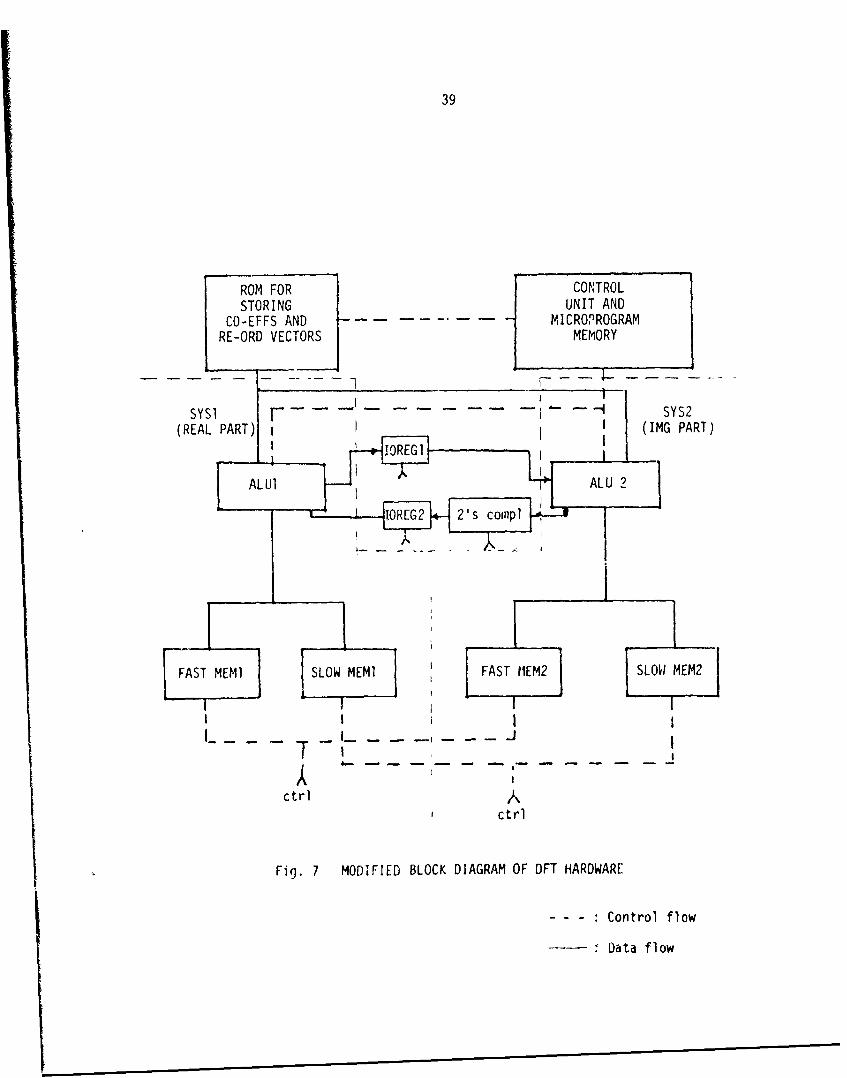
The coefficients in the PFA are either purely real or purely imaginary.
This fact can be used to speedup the system further by using an extra arith-
metic and logic unit (ALU). The width of microinstruction will have to be
increased by a few bits to generate the additional control signals needed.
A modified block diagram is shown in Fig. 7. The real and imaginary parts
of the data are processed separately. Whenever the coefficient to be multi-
plied is real, there will not be any interaction between the two ALU's, but
if the coefficient is imaginary, the results after the multiplication are
exchanged between the two ALU's.
Two I/O registers IOREGI and IOREG2 are used for this purpose. The ALUI
and ALU2 can load registers IOREGI and IOREG2, and read from registers IOREG2
and IOREGI respectively. The system shown in Fig. 7 can be thought of as two
identical processors working in parallel and controlled by a single controller
(CCU). The addresses of IOREGI and IOREG2 for SYSI are identical to the addres-
ses of registers IOREG2 and IOREGI respectively, for SYS2. The other blocks
in Pig. 7 are self-expldnatory.
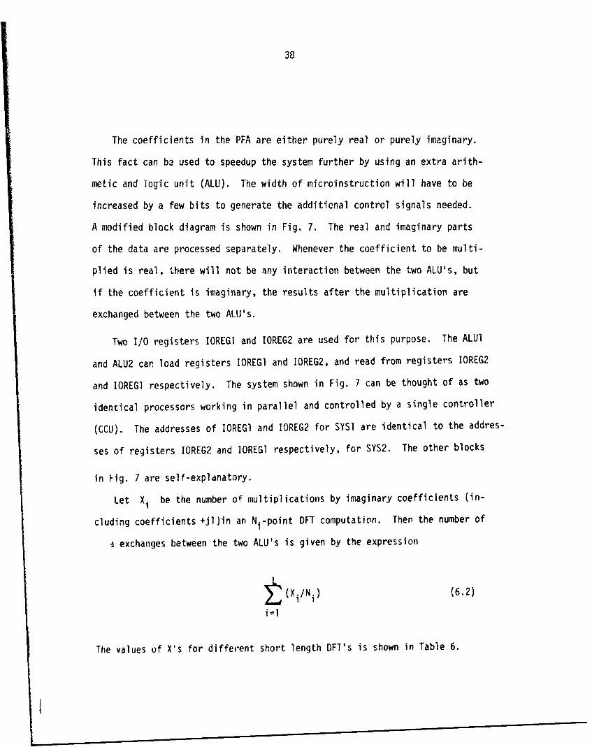
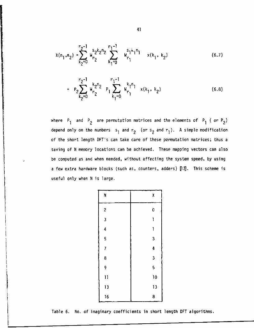
Let Xi be the number of multiplications by imaginary coefficients (in-
cluding coefficients +jl)in an Ni-point DFT computation. Then the number of
d exchanges between the two ALU's is given by the expression
(Xi/N) d 6.2)
i=l
The values of X's for different short length DFT's is shown in Table 6.
39
ROM FOR CONTROLSTORING UNIT AND
CO-EFFS AND MICROPROGRAMRE-ORD VECTORS MEMORY
SYSI I - •SYS2
(REAL PART) i(IMG PART
ALUI ALU 2
,TRG 2's compl
ctrl
C ti-i
ctrtrl
Fig. 7 MODIFIED BLOCK DIAGRAM OF OFT HARDWARE
- - - :Control flow
Data flow
40
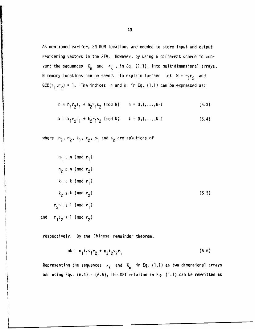
As mentioned earlier, 2N ROM locations are needed to store input and output
reordering vectors in the PFA. However, by using a different scheme to con-
vert the sequences Xn and xk , in Eq. (1.1), into multidimensional arrays,
N memory locations can be saved. To explain further let N = r 1 r 2 and
GCD(rl,r 2 ) = 1. The indices n and k in Eq. (1.1) can be expressed as:
2 n1 r2sI + n2rIs2 (mod N) n = O,l,...,N-1 (6.3)
k k klr 2sI + k2 r 1 s2 (mod N) k = 0,1,...,N-1 (6.4)
where nl, n2 , k1, k2, sI and s2 are solutions of
nI 1 n (mod r 1 )
n -n (mod r 2 )
kE 1 k (mod r1 )
k2 - k (mod r 2) (6.5)
2s 1 (mod r1 )
and rls 2 I (mod r 2 )
respectively. By the Chinese remainder theorem,
nk 7 n kIsIr 2 + n2k2s 2 r1 (6.6)
Representing the sequences xk and X in Eq. (1.1) as two dimensional arrays
and using Eqs. (6.4) - (6.6), the OFT relation in Eq. (1.1) can be rewritten as
41
r2-1 rl-I
X~n1,2) =~ s2 k2n2 k wlg..O.lInl(67X(nlSn r2) -1 W s2k2n2r2=- Wrln x(kI, .k) (6.7)
k2=0 2 kI=xl0 kln
r2- kn ri1 k n
P2E Wr p, W 1 1 x(kI, k2 ) (6.8)
k2=0 2 k1=0
where P1 and P2 are permutation matrices and the elements of P1 ( or P2 )
depend only on the numbers sI and r 2 (or s2 and rl). A simple modification
of the short length DFT's can take care of these permutation matrices; thus a
saving of N memory locations can be achieved. These mapping vectors can also
be computed as and when needed, without affecting the system speed, by using
a few extra hardware blocks (such as, counters, adders) 03]. This scheme is
useful only when N is large.
N X
2 0
3 1
4 1
5 3
7 4
8 3
9 5
11 10
13 13
16 8
Table 6. No. of imaginary coefficients in short length DFT algorithms.
42
CONCLUSION
Efficient algorithms exist for computing the DFT of long sequences, when
the sequence length is a composite number. The FFT, the PFA and the WFTA are
three such algorithms. In this report, various aspects of these algorithms
were discussed. Efficient algorithms for 11 and 13-point DFT's were pre-
sented. Using these and the other short length transforms, the DFT of very
long sequences can be obtained by the PFA and the WFTA, in fewer number of
multiplications than in the FFT.
In the PFA, the DFT of a long sequence is obtained by performing a number
of short length DFT's. This fact can be used to design high-speed dedicated
hardware for DFT computation. Moreover, the PFA requires fewer arithmetic
operations (i.e., combined additions and multiplications). Hence, it is
expected to introduce smaller error due to finite word length arithmetic.
The FFT requires fewer additions than the other two algorithms, but the
number of multiplications needed is considerably greater. It is, however,
important to note that the FFT lends itself to more systematic programming.
The WFTA requires the least number of multiplications among the three
algorithms. However, the number of additions required is slightly more than
the others for transform sizes up to few thousands and becomes formidable
for very long transforms. Furthermore, it requires more data and program
memory than is required for the other two.
43
REFERENCES
1. A. V. Oppenheini and R. W. Schafer, Digital Signal Processing, Englewood
Cliffs, NJ: Prentice Hall, 1975, pp. 285-328.
2. S. Winograd, "A new method for computing DFT", Proc. of IEEE Int. Conf.
on ASSP, May 1977, pp. 366-368.
3. H. F. Silverman, "An Introduction to Programming the Winograd Fourier
Transform Algorithms (WFTA)", IEEE Trans. on ASSP, May 1977, pp. 152-165.
4. D P. Kolba and T. W. Parks, "A Prime Factor FFT Algorithm using High
Speed convolutions", IEEE Trans. on ASSP, Aug. 1977, pp. 281-291.
5. L. R. Rabiner and B. Gold, Theory and Application of Digital Signal Proces-
sing, Englewood Cliffs, NJ: Prentice Hall, 1975.
6. J. W. Cooley and J. W. Tuckey, "An Algorithm for machine calculation of
Complex Fouier Series," Math. of Comput., Vol 19, April 1965, pp. 297-301.
7. I, J. Good, "The interaction algorithm and practical Fourier analysis",
J. Royal Statistical Society, Ser. B. Vol. 20, 1958, pp. 361-372.
8. C. Rader, "Discrete Fourier Transform when the number of data samples is
prime", Prec. of the IEEE, Vol 56, June 1968, pp. 1107-1108.
9. S. Winograd, "On Computing the discrete Fourier transform", Proc. Nat.
Acad. Sci., USA, Vol 73, No. 4, April 1976, pp. 1005-1006.
00. S. Winograd, "Some bilinear forms whose multiplicative complexity depends
on the field of constants", IBM Research Report, RC 5669, Walson Research
Center, N.Y., Oct. 1975.
11. P.D. Welch, "A fixed point fast Fourier transform error analysis", IEEE
Trans. on Audio Electro Acoust., Vol. AV-17, June 1969, pp. 151-157.
44
12. Tan-Thoung and Bede Liu, "Fixed Point fast Fourier transform analysis",
IEEE Trans. on ASSP, Vol. 24, Dec. 1976, pp. 563-573.
13. W.K. Jenkins and B.J. Leon, "The use of Residue Number Systems in the
design of finite impulse response digital filters", IEEE Trans. on
Circuits and Systems, Vol. CAS-24, April 1977, pp. 191-200.

45
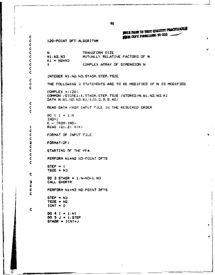
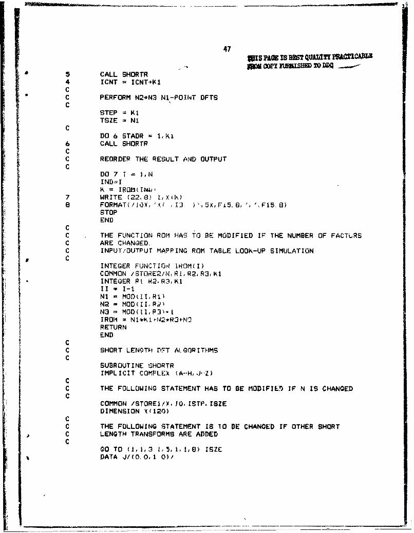
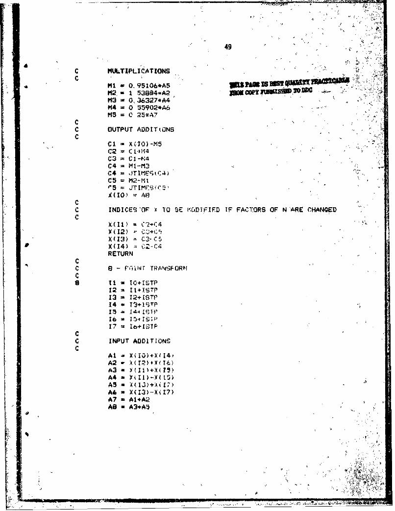
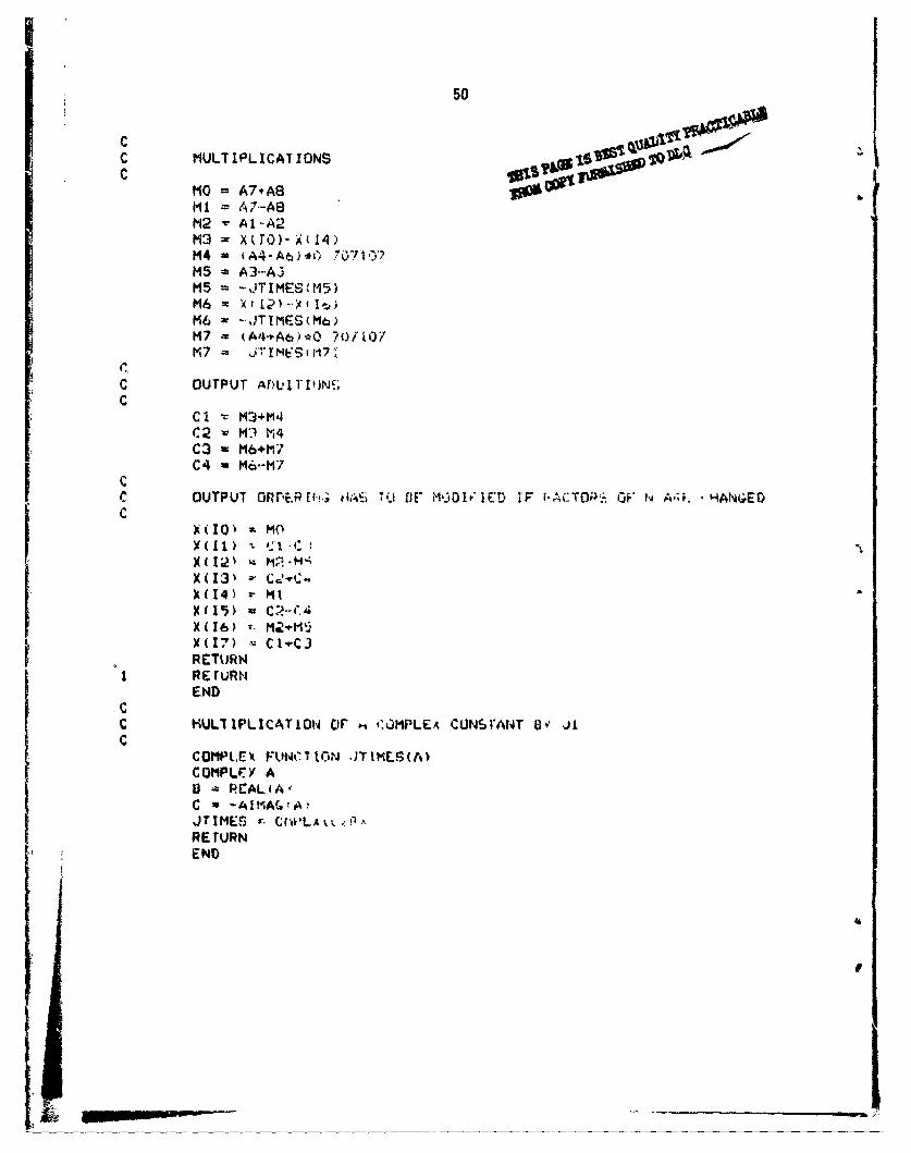
APPENDIX
This Appendix lists a FORTRAN program for obtaining the DFT of 120-points,
by the PFA. By making minor modifications at the places indicated, this pro-
gram can be used to implement all the 3-factor PFA's.
46
C P15 rPAU~ to DDAC 120-POINT DFT ALGORITHMCCC N "TRANSFORM SIZEC N1, N2, N3 MUTUALLY RELATIVE FACTORS OF NC K1 = N2*N3C X COMPLEX ARRAY OF DIMENSION NCC
INTEGER Ni, N2, N3, STADR, STEP. TSZECC THE FOLLOWING 3i STATEM4ENTS ARE TO HE MODIFIED IF N IS MODIFIEDC
COMPLEX X(120)COMMON /STC,,EI/X STADR,. STEP, TSZE /STORE2/N, Ni, N2, N3, fK1DATA N, N1, t42, N3, K1iI 210, 3,5,E,40/
C READ DATA FROM INPUT' FILE IN THE REUIRED ORDERC
DO I i = i,N
IND-.'K 6ý ROMi LND)
I READ (201,2) X(K,)
CC FORMAT OF INPUT FILE
C2 FORMAT(2F)CC STARTING OF THE PFACC PERFORM NI*N2 143-POINT DFTSC
STEP w I
TSZE w N3C
DO 3 STADR = 1.N-N3+1.N33 CALL SHORTRCC PERFORM NI*N3 N2-POTNT DFTSc
STEP - N3
TSZE - N2ICNT - 0
DO 4 1 . 1,NI
DO 5 J a 1,STEPSTADR a ICNT+J
47
"5 CALL SHORTR
4 ICNT = ICNT+KIC"C PERFORM N2.N3 N1-POI1T DFTS
STEP = K1
TSZE = NIC
DO 6 STADR = 1,Ki6 CALL SHORTRCC REORDER THE RESULT AND OUTPUTC
DO 7T -= 1,NIND=II P~K = %RttNi7 WRITE (226,8) I,Xtk)
8 FORMAT(/OX, .. •( ,I', ,",3x,F,5.8, ', '.F15.8)STOPEND
C
C THE FUNCTION ROM HASS TlO BE MODIFIED IF THE NUMBER OF FACTLRSc ARE CHANGED.
C INPUT/OUTPUT MAPPING ROM TABLE LOOK-VP SIMULATIONw C
INTEGER FUN-CTION IROM(I)
COMMON /STQ)RE2/N, RI, R2o R3, Kl1INTEGER Rl $•2,R3,KlII I-1
Ni - MOD(IT,RIlN2 - MOD(II..?N3 - MOD(TI,P3ý"IIROII = NI*KleIJ2*R3+H2.N2RETURNEND
CC SHORT LENGTH EM-T Al. GOPITHMSC
SUBROUTINE SHORTRIMPLICIT COMPLE'X (A-H,.J"Z)
C THE FOLLOWING STATEMENT HAS TO BE MODIFILD IF N IS CHANGED
CCOMMON /STOREl/Y, ,I, TP. ISZEDIMENSION X(120)
cC THE FOLLOWING STATEMENT IS 10 BE CHANOED IF OTHER SHORTC LENGTH TRANSFORMS ARE ADDEDC
GO TO (1,1,3 1, ,1,1, 8) ISZEDATA J/(O,O, 1 0)#
____ __ ______ _ __ ___

48
C Ins PAgs Is an ckuwA mama
C 3-POINT DFT OW t
C3 I1 = IO+ISTP
12 = I1+ISTPCC INPUT ADDITIONSC
At a X(11)+X(I2)A2 = X(Il)-X(12)A3 - X(IO)+A1
CC MULTIPLICATIONSC
M1 = 0. 5*AlM2 = 0 86603A2
CC OUTPUT ADDITIONSCC OUTPUT ORDERIN:1i HAS TO BE MODIFIED IF FACTORS OF 14 ARE OHANOEDC
Cl = X(IO)-M1X(lO) - A'JM2 = -JTIMES(M2)X(ll) z C I +-J2w
X(12) = CI-JM2RETURN
CC 5 - POINT DFTC5 It - IO÷ISTP
12 = II+ISTP13 = 12+ISTP14 = 13+12TP
CC INPUT ADDITIONSC
Al = X(I1)+x(14)A2 - X(II)-X(14)
A3 = X(12)+X(13)A4 - X(12)-Xt13)A5 = A2+A4A6 = Al-'A3A7 a Al+A3
i AS w X(IO)+A7
Ov
i'Ir1
44
C NULT-lPLICATXON.S
C M- 0. 95106*AS-
M12, I 53884*A2143 - 0. 36327*A4'M14 - 0 ~5S92*A6M15 -0 2--*A7
CC OUTPUT AMMITONSC
Cl -X(270)-m5C2= C I f M4
C3 =C1-1-'404 = M1-M3C4 = TMct4
c INIE*FXT 5 WFF)I FACTORS OF N ARC CHANGED
RETURN
11 TO.YcVTP
14 TAJ+1CSTP115 14- ITV316 - 1 t'1S
C INPUT ADDITIONS
A3 -c ~A4 = - l-(5
AS *A6 = X(13)-'X(17)A7 - A1.A2AS= A~3+A5~
50
C ~MULTIPLICATIONS s"Tow
MO =A71ABHl = 7.-ABM2 -Al -A2M3= X(10)- i(14)
M4 - A4-Ab)*40 70-!1,')7M5 lAM5 =-JTIMESý'M5)
M6 - XIl )-xII?Mw -JTlM*ES(M6)
M7 - A4i-Abi-tO ?OilOl~M7 Vlq3 i7''
41C OUTPUT AT tjTIfNW.C
Cl M13+M4C2 - l M'4C~3- 6MC4 -M6--M7
cIc OUTPUT O~. [I-!; OA.; Tij Bf3 olDo IE.D IF i-ACTOP*' OF W A4.T HANGEDC
X 'ol- MO
Y(11) ~-% '' q : I
X(17) -u C trC3RETURN
I R~rURNEND
cC KUL71PLICATION orV COMPLE& CUNSEANT Ov JI
COMPL.EX FU'NCT trN Jr IMLS(A)CQMPLVY A13 PCALfAlC *-AJllAG:A,JTIMEf) :. CF.LAU.,r-RErURNEND