Embed Size (px)
Citation preview

CENTER FOR
MACHINE PERCEPTION
CZECH TECHNICAL
UNIVERSITY
RE
SE
AR
CH
RE
PO
RT
ISS
N12
13-2
365
Omnivergent Stereo-panoramaswith a Fish-eye Lens
(Version 1.0)
Hynek Bakstein and Tomas Pajdla
[email protected], [email protected]
CTU–CMP–2001–22
Available atftp://cmp.felk.cvut.cz/pub/cmp/articles/bakstein/Bakstein-TR-2001-22.pdf
This research was supported by the following grants: GACR102/01/0971, EU Fifth Framework Programme project OMNIVIEWS
IST-1999-29017, MSMT KONTAKT 2001/09, and MSMT 212300013.
Research Reports of CMP, Czech Technical University in Prague, No. 22, 2001
Published by
Center for Machine Perception, Department of CyberneticsFaculty of Electrical Engineering, Czech Technical University
Technicka 2, 166 27 Prague 6, Czech Republicfax +420 2 2435 7385, phone +420 2 2435 7637, www: http://cmp.felk.cvut.cz

Omnivergent Stereo-panoramas with a Fish-eye Lens
Hynek Bakstein and Tomas Pajdla
Abstract
We present a novel approach to the calibration of an ultra wide angle fisheye lenses. These lenses have the field of view larger than180◦, therefore thecommon calibration methods based on the classical pinhole camera modelwith a planar retina cannot be employed. A new camera model is proposedtogether with a calibration method for extracting its parameters. Experi-ments evaluating the proposed technique are presented. We also present anexample of a camera that can be described by the proposed model and cali-brated by the proposed method. It consists of a standard of-the-shelf fish eyeadapter from Nikon and a common CCD camera. Possible fields of employ-ment of this sensor include construction of 360 x 360 mosaics.
1. Introduction
Large field of view (FOV) is useful or even mandatory for some computer visionapplications. Larger FOV assures that more points are visible in one image, whichis good for algorithms for the 3D reconstruction. Several ways to enlarge the FOVexist. Mirrors, lenses, moving parts, or a combination of the previous can be em-ployed for this purpose. In this paper we focus on the use of a special lens, theNikon FC-E8 fish eye converter [3], which provides FOV of183◦. Such a sensorcan be used in a practical realization of the 360 x 360 mosaics [7].
The 360 x 360 mosaic is a good example of a noncentral camera where the lightrays are tangent to a circle, see Figure 1. Let us describe the geometry of the lightrays that form the mosaic. A planeπ is rotated on a circular pathC with a radiusr.The planeπ is perpendicular to the planeδ and moreover, it is tangent to the circleC. At each rotation position, all light rays lie in the planeπ and intersect the pointwhere the planeπ touches the circleC. Because each point outside the circleC canbe observed by two light rays, the camera provides a complete spherical mosaicfor both the left and the right eye after a rotation of the planeπ about360◦. Oneimportant property of the 360 x 360 mosaic is that it produces a pair of two stereoimages where the corresponding points lie on the same image row. This simplifiesthe correspondence search to a one dimensional search along the lines.
1

r
π
�
δ
Figure 1: Geometry of 360 x 360 mosaic.
Let us mention two possible realizations of the 360 x 360 mosaics. One re-quires a mirror, which can be either conical observed by a telecentric lens (de-picted in Figure 2(a)), or of a specially designed shape observed by a classicalpinhole camera [7]. Other realization can be made with an easily available off theshelf Nikon fish eye converter with the FOV equal to183◦. The points in the im-age corresponding to the light rays lying in the planeπ have to be selected at eachrotation step from the image. Therefore, the lens has to be calibrated.
(a) (b)
Figure 2: Two possible realizations of the 360 x 360 mosaic. (a) a telecentriccamera and a conical mirror, (b) a central camera with Nikon fish eye converter.
Methods for the calibration of wide angle lenses that can be found in the liter-ature [1, 13, 12, 2] assume that the corrected image can be unwarped to a planar
2

retina. That is not possible with the FOV larger than180◦ where a spherical retinahas to be used instead. A new omnidirectional central camera model has to beproposed.
The structure of the paper is as follows. In Section 2 we propose the cameramodel. A method for estimating its parameters is then presented in Section 3.Experimental results can be found in Section 4.
2. Camera model
The main gist of our novel approach is that a planar retina cannot be used in themodel of an omnidirectional camera. Let us adopt the definition of the omnidirec-tional camera from [8]:An image is directional iff there exists vectoru ∈ <3 suchthat ux > 0 for all vectorsx pointing from the camera center towards the scenepoints. We say that the image is omnidirectional if there is no suchu. Image ob-tained by a183◦ FOV FC-E8 lenses can be omnidirectional. Therefore, we cannotconstruct the light rays in the camera coordinate system like in the directional caseby adding a unitz coordinate to point coordinates in the image plane(u, v), seeFigure 3(a). The light rays have to be constructed in a truly omnidirectional way,by transforming the image plane coordinates(u, v) into coordinates(x, y, z) of raydirections vectors expressed with respect to some camera coordinate system, as itis depicted in Figure 3(b).
(u,v) (u,v)
a) b)
Figure 3: From image coordinates to light rays: (a) a directional and (b) an omni-directional camera.
3

By a camera model we understand the mapping from image points to rays thatpass through the camera center. What is the camera model of a single CCD imageobtained with the FC-E8 lens? Figure 4 shows a plane with concentric circlesplaced in front of the lens. The center of the circles is placed approximately intothe center of the image. The radii of the circles equalR tan θ, whereθ is the anglebetween the camera rays passing through the points on the circle and the opticalaxis of the lens andR is the distance of the plane with circles from the cameracenter. We can notice that the circles image to circles and that they have a constantstep in their radii, measured from the image center. Therefore we can formulate theobservation that there is alinear relationship between the angleθ and the radiusr of a point in the image. We have verified these observations experimentally, seeFigures 7-9. These figures show dependence of the radiusr on the angleθ. Noticethat the function is almost linear, however, its first and second derivatives show thatit can be more precisely approximated by a polynomial function. We will discussthis fact later.
Figure 4: Image of circles with radii set to a tangent of a constantly incrementedangle results in concentric circles with a constant increment in radii in the image.
Let (u, v) denote coordinates of a point in the image measured in an orthogonalbasis as shown in Figure 5. CCD chips often have a different distance betweenthe cells in the vertical and the horizontal direction. This results in a distortionbecause the image is not scaled equally in the horizontal and vertical direction.Therefore, we introduce a parameterβ representing the ratio between the scales ofthe horizontal respectively the vertical axis. This distortion causes the circles to
4

appear as ellipses in the image, as shown in Figure 5. A matrix expression of thedistortion can be written in the following form:
K−1 =
1 0 −u0
0 β −βv0
0 0 1
. (1)
This matrix is a simplified intrinsic calibration matrix of a pinhole camera [5].The displacement of the center of the image is expressed by termsu0 andv0, theskewness of the image axes is neglected in our case, because we suppose that ourcamera has orthogonal pixels.
K−1
v
u u’
v’
Figure 5: A circle in the image plane is distorted due to a different length of theaxes. Therefore we observe an ellipse instead of a circle in the image.
Under the above observations, we can formulate the model of the camera. Pro-vided with coordinates of some image point(u, v, 1)T , we are able to computetheir rectified image coordinatesu′ = (u′, v′, 1)T by the multiplication byK−1
u′ = K−1u . (2)
We can compute the corresponding polar coordinates with respect to the center ofthe distortion(0, 0), that is the radiusr of the circle on which the point lies andthe angleϕ between the point and theu′ axis of the image coordinate system, seeFigure 6(a).
The radiusr can be computed as
r =√
(u′)2 + (v′)2 . (3)
The angleϕ is then expressed as
ϕ = atan2(u′, v′) . (4)
5

u’
v’(u’,v’)
r
ϕ(u’ ,v’ )00
θ
x
y
(x’,y’,z’)
z = optical axis
ϕ
(a) (b)
Figure 6: (a) From orthogonal coordinates(u′, v′) to polar coordinates(r, ϕ). (b)Camera coordinate system and its relation to the anglesθ andϕ.
The value ofr determines the angleθ between the light ray in the cameracentered coordinate system and the FC-E8 optical axis (which is equal to thez axisof the camera centered coordinate system). We have observed that this relationis approximately linear and can be more precisely expressed as a polynomial ofthe third degree. See Figure 7 for the graph of the dependence of the radiusr ofan image point on the angleθ and Figure 8 and Figure 9 for its first and secondderivatives which were estimated using finite differences. Notice that the secondderivative is a linear function and therefore the polynomial has degree equal tothree.
Now we are ready to express the angleθ as a function ofr:
θ = ar3 + br2 + cr , (5)
wherea, b, andc are unknown coefficients of the polynomial. Provided withϕ, θ,andr, the light rayx′ = (x′, y′, z′)T in the camera centered coordinate frame canbe computed as
x′ =
x′
y′
z′
=
sin θ cos ϕsin θ sinϕ
cos θ
, (6)
as it is depicted in Figure 6(b).Directionsx′ are determined by six parameters, the image center(u0, v0), the
three polynomial coefficients, andβ. These parameters can be estimated fromunknown lines in the scene without the full metric calibration of the camera. Fora metric camera calibration, a known scene with calibration points measured withrespect to some scene coordinate systems is required.
6

−100 −50 0 50 100−500
0
500
θ
r(θ)
Measured pointsCubic fit
Figure 7: Dependence of ther(θ) coordinate of a point on angleθ.
−100 −50 0 50 100−50.5
−50
−49.5
−49
−48.5
−48
−47.5
−47
−46.5
−46
θ
Firs
t der
ivat
ive
of r
(θ)
Measured pointsQuadratic fit
Figure 8: Dependence of the first derivative of ther(θ) coordinate of a point onangleθ.
7

−100 −50 0 50 100−2
−1.5
−1
−0.5
0
0.5
1
1.5
θ
Measured pointsLine fit
Figure 9: Dependence of the second derivative of ther(θ) coordinate of a point onangleθ.
Denoting the scene coordinates of the calibration points byX = (x, y, z)T ,we can express their coordinates in the camera centered coordinate system asX =(x, y, z)T by equation
X = RX + T , (7)
whereR represents a rotation andT stands for a translation. The matrixR hasthree degrees of freedom and the vectorT = (t1, t2, t3)T is expressed by threeparameters. This yields us six unknown parameters. Together with the imagecenter, three parameters for the non-linear distortion camera, and the parameterβ,we are left with twelve unknowns.
3. Estimation of the model parameters
The camera can be calibrated from a known scene. However, to eliminate thenonlinear distortion, we need to observe only a set of straight lines similarily asit was done for perspective cameras [9]. After determining the parameters of thetransformation projecting the straight lines in the scene to curves we obtain aninternally calibrated omnidirectional central camera.
Full calibration, which means the estimation of the intrinsic parameters (theimage center andβ), the nonlinear distortion, and the extrinsic parameters [4], canbe performed under knowledge of known points in the scene and their correspond-ing images. Figure 11(a) shows the scene, which was used during our experimentsand Figure 11(b) contains images of these points. Note that the middle lines of thepoints in both directions go through the center of the image (marked by ’+’). The
8

green circle illustrated the field of view of an fish eye image and the blue ellipsemarks points corresponding to the light rays which lie in the planeπ.
030
6090
120
−100
0
100
−200
−100
0
100
200
0 200 400 600 800 1000
100
200
300
400
500
600
700
800
900
u
v
(a) (b)
Figure 10: (a) Points in the scene, the black dot denotes the camera center, and (b)their images, where the ’+’ is the image center.
3.1. Calibration of internal parameters
The main idea of an elimination of the nonlinear distortion is based on the fact, thatthe light rays respective to points lying on a line in the scene span a two dimensionalsubspace of the three dimensional scene space. Therefore, if we write down theircoordinates in a matrix form
Aj =
x1 x2 . . . xn
y1 y2 . . . yn
z1 z2 . . . zn
, (8)
wheren is the number of points on a line andj = 1..l, wherel denotes the numberof the lines, the matrixAj should have rank 2. Moreover, the autocorrelationmatrix
Bj = AjAjT (9)
has to be of rank 2 as well. Therefore we can formulate an objective function
J =l∑
j=1
(λj3)
2 , (10)
9

whereλj3 is the smallest eigenvalue of the matrixBj . We minimize this function
with respect to the six parameters (the image center,β, and the three polynomialcoefficients) used to compute the light rays in (6).
3.2. Complete camera calibration
Putting together all parameters described at the end of Section 2 we are left withtwelve unknown parameters to estimate. We define the objective function
J =N∑
i=1
∥∥∥∥∥ X‖X‖
− x′
‖x′‖
∥∥∥∥∥ , (11)
where‖...‖ denotes the Euclidean norm andN is the number of points. This func-tion closely approximates the angle between the rays provided by the camera modeland the true ones. A MATLAB implementation of the Levenberg-Marquardt [6]minimization was employed in order to minimize the objective function (11).
4. Experimental results
In this section we show the experiments verifying each step of the proposed cali-bration method. Our experimental setup is shown in Figure 11(a). It consisted of aPulnix TM-1001 camera with a standard 12.5mm lens on which the Nikon fish eyeconverter FC-E8 was mounted. The camera was placed on a motorized turntable.Seven calibration points in one line were deployed in the scene. The turntable wasrotated from−90◦ to 90◦ with a step of10◦. Therefore a set of 19 images wasacquired. In Figure 11(b), you can see one of the images.
(a) (b)
Figure 11: (a) experimental setup and (b) one of the images in the sequence usedfor calibration showing the seven points in one row.
10

We can create a scene with all the points composing a 3D object instead of aline if we fix a scene coordinate system to one orientation of the camera and forits each rotation we compute the coordinates of the calibration points with respectto this fixed coordinate system. The points in the scene will lie on a cylinder, seeFigure 10(a). We will refer to the line of 7 points corresponding to points acquiredat one rotation step, and therefore one image, by the termcolumnof points. We canalso create an image of all these points by composing their coordinates detected ineach of the 19 images into one synthetic image, as it is depicted in Figure 10(b).We will use this artificial scene in some of the following experiments. However,a the axis of rotation does not have to be axactly in the centre of projection of thecamera. Then, the camera will not only rotate, but move along a circle. This doesnot change the scene coordinates of the points on the cylinder, instead it influencesthe translation of the camera with respect to the scene coordinate system by thevalue of the radius of the circle on which is the camera rotated.
First, we show that provided with image coordinates of some points we areable to determine the intrinsic parameters of our camera, that is the image center,β, and the coefficients of the polynomial defined in (5). We set the image center tothe center of the circular image formed by the lens. The parameterβ was set to 1and the polynomial coefficients values were set to an initial fit obtained from oneline of points in the image passing through the distortion center, as it is shown inFigure 7. A line fit error, that is the smallest eigenvalue of the matrixBj from (9)for this initial guess of the parameters and after the optimization of these param-eters (described in Section 3.1) is depicted in Figure 12(a). Note the significantdecrease of the line fit error.
0 5 10 15 200
0.5
1
1.5
2
2.5
3
3.5
4
4.5x 10
−4
Line number
Line
fit e
rror
Initial estimate Nonlinear correction (Section 3.1)
0 10 20 30 40 50 60 700
0.05
0.1
0.15
0.2
Calibration point
Cal
ibra
tion
erro
r
Nonlinear correction (Section 3.1)Full optimization (Section 3.2)
(a) (b)
Figure 12: (a) The line fit error for all 19 lines. (b) The calibration error (thedistance betweenX andX′) for odd calibration points.
11
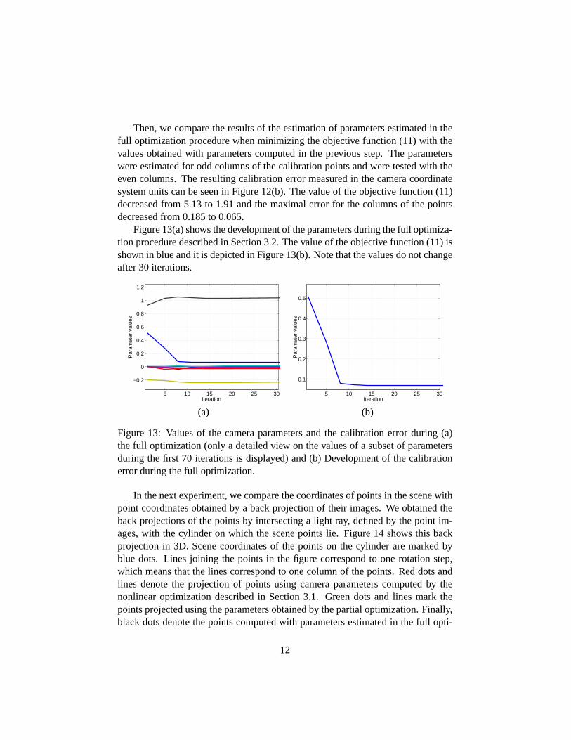
Then, we compare the results of the estimation of parameters estimated in thefull optimization procedure when minimizing the objective function (11) with thevalues obtained with parameters computed in the previous step. The parameterswere estimated for odd columns of the calibration points and were tested with theeven columns. The resulting calibration error measured in the camera coordinatesystem units can be seen in Figure 12(b). The value of the objective function (11)decreased from 5.13 to 1.91 and the maximal error for the columns of the pointsdecreased from 0.185 to 0.065.
Figure 13(a) shows the development of the parameters during the full optimiza-tion procedure described in Section 3.2. The value of the objective function (11) isshown in blue and it is depicted in Figure 13(b). Note that the values do not changeafter 30 iterations.
5 10 15 20 25 30
−0.2
0
0.2
0.4
0.6
0.8
1
1.2
Iteration
Par
amet
er v
alue
s
5 10 15 20 25 30
0.1
0.2
0.3
0.4
0.5
Iteration
Par
amet
er v
alue
s
(a) (b)
Figure 13: Values of the camera parameters and the calibration error during (a)the full optimization (only a detailed view on the values of a subset of parametersduring the first 70 iterations is displayed) and (b) Development of the calibrationerror during the full optimization.
In the next experiment, we compare the coordinates of points in the scene withpoint coordinates obtained by a back projection of their images. We obtained theback projections of the points by intersecting a light ray, defined by the point im-ages, with the cylinder on which the scene points lie. Figure 14 shows this backprojection in 3D. Scene coordinates of the points on the cylinder are marked byblue dots. Lines joining the points in the figure correspond to one rotation step,which means that the lines correspond to one column of the points. Red dots andlines denote the projection of points using camera parameters computed by thenonlinear optimization described in Section 3.1. Green dots and lines mark thepoints projected using the parameters obtained by the partial optimization. Finally,black dots denote the points computed with parameters estimated in the full opti-
12

mization procedure, described in Section 3.2. Note that the points projected usingthe parameters estimated in the nonlinear optimization (Section 3.1) have a signifi-cant reprojection error. However, both the partial and the full optimization broughtthe points closer to the measured coordinates.
−200−100
0100
200
−200
−100
0
100
200
−200
−100
0
100
200
300
Figure 14: Back projection of detected points to the scene with parameters obtainedfrom the nonlinear optimization (Section 3.1), the partial optimization and the fulloptimization (Section 3.2).
For better clarity, we illustrate the back projection of the points to the sceneon a cylinder unwarped to a plane. Figure 15 show the comparison between thepoints back projected using the parameters estimated in the nonlinear optimization(Section 3.1). Note a rotation of the points. Figure 16 shows the same situationsas above but in this case, the points back projected employing the parameters es-timated in the full optimization (Section 3.2) were used. The lines joining themeasured and back projected points were scaled in Figure 17 for better illustrationof the calibration error. Note that there is still some systematic distortion. Thenature of this eeror has to be still found.
Finally we show that we are able to select an ellipse corresponding to lightrays lying in the planeπ. The angle between these rays and the optical axis is
13

0 50 100 150 200 250 300 350 400 450−300
−200
−100
0
100
200
300
400
Figure 15: Back projection of detected points to the scene with the parametersobtained from the nonlinear optimization (Section 3.1). The results are displayedon a cylinder unrolled to a plane, the blue ’x’ denotes the measured points and thered ’+’ marks the reprojected points. Red lines joining the corresponding pointsillustrate the reprojection error.
π2 , therefore we have to select points which have the angleθ (see (5)) equal toπ2 .This step is crucial for the employment of the proposed sensor in a realization of the360 x 360 mosaic. The selection of the proper ellipse assures that the correspondingpoints in the mosaic pair will be on the same image rows, which simplifies thecorrespondence search algorithms.
Figures 18 and 19 show the right and the left eye mosaic respectively. Note thesignificant disparity of objects in the scene. Five examples of corresponding pointsare marked by yellow ’x’. Enlarged parts of the mosaic showing one correspondingpoint can be found in Figures 20(a) for right mosaic and Figures 20(b) for the leftmosaic. Notice that the points lie on the same image row.
14

0 50 100 150 200 250 300 350 400 450−300
−200
−100
0
100
200
300
Figure 16: Back projection of detected points to the scene with the parametersobtained from the full optimization (Section 3.2). The results are displayed on acylinder unrolled to a plane, the blue ’x’ denotes the measured points. Black linesjoining the corresponding points illustrate the reprojection error.
5. Conclusion and outlook
We have proposed a novel camera model and a method for estimating its parame-ters. This model describes optics which can be used in a realization of the 360 x 360mosaics. This realization uses standard off the shelf components and does notrequire a mirror, thus simplifying the design of the 360 x 360 mosaics camera.Experimental results verify that the model describes the real camera and that theparameters can be recovered with a reasonable precision.
However, there are some questions open. How many lines are needed to esti-mate the parameters of the nonlinear distortion and what are the degenerate cases?What is the number of points required for the full calibration? Also, we wouldlike to test our sensor with some dense stereo reconstruction algorithm, for exam-ple [10]. Mosaic images obtained with our camera are rectified and therefore the
15

0 50 100 150 200 250 300 350 400 450−300
−200
−100
0
100
200
300
Figure 17: Back projection of detected points to the scene with the parametersobtained from the full optimization (Section 3.2). The results are displayed on acylinder unrolled to a plane, the blue ’x’ denotes the measured points. Black linesjoining the corresponding points, illustrating the reprojection error, were scaled 2.5times.
employment of such an algorithm should be straightforward, however, it has to beadapted to reflect the topology of the mosaic images, which is the torus [11].
References
[1] A. Basu and S. Licardie. Alternative models for fish-eye lenses.PatternRecognition Letters, 16(4):433–441, 1995.
[2] S. S. Beauchemin, R. Bajcsy, and Givaty G. A unified procedure for calibrat-ing intrinsic parameters of fish-eye lenses. InVision Interface (VI 99), pages272–279, May 1999.
[3] Nikon Corp. Nikon www pages: http://www.nikon.com, 2000.
16
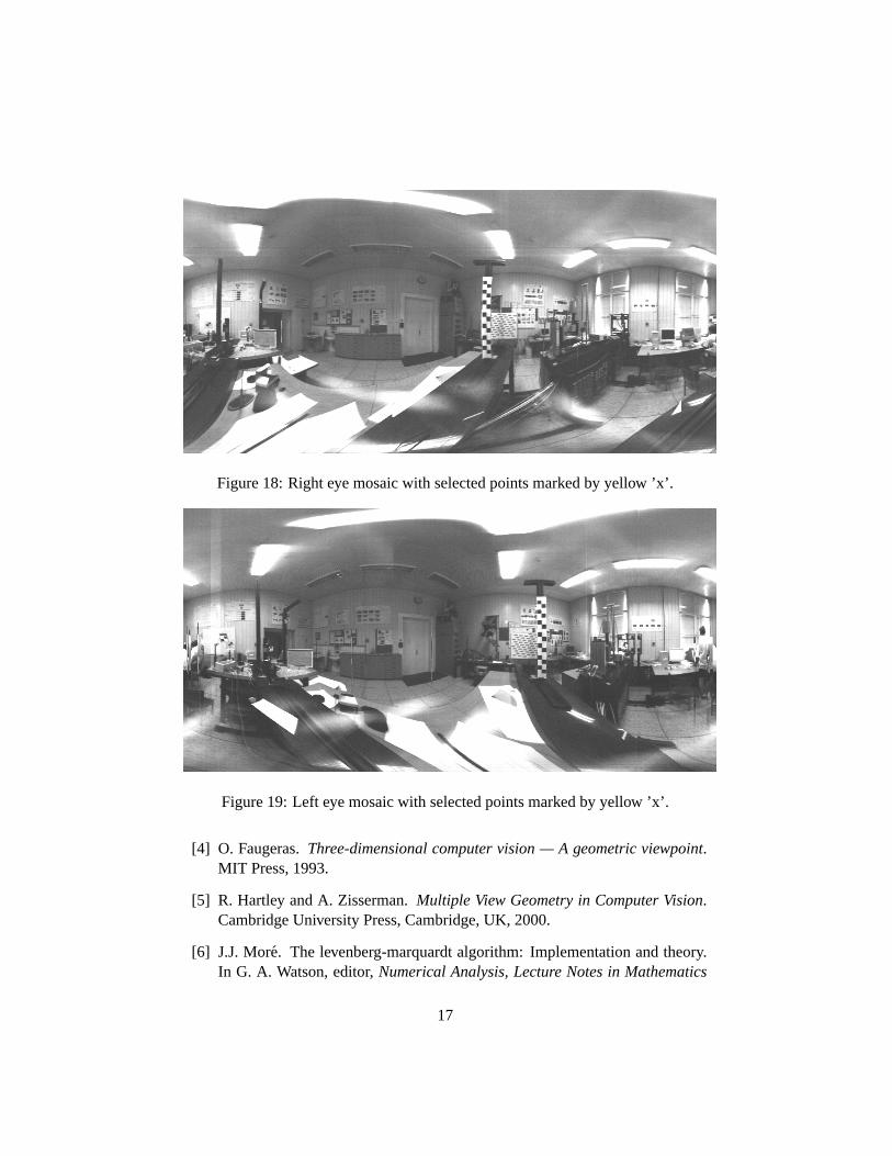
Figure 18: Right eye mosaic with selected points marked by yellow ’x’.
Figure 19: Left eye mosaic with selected points marked by yellow ’x’.
[4] O. Faugeras.Three-dimensional computer vision — A geometric viewpoint.MIT Press, 1993.
[5] R. Hartley and A. Zisserman.Multiple View Geometry in Computer Vision.Cambridge University Press, Cambridge, UK, 2000.
[6] J.J. More. The levenberg-marquardt algorithm: Implementation and theory.In G. A. Watson, editor,Numerical Analysis, Lecture Notes in Mathematics
17

(a) (b)
Figure 20: Detail of one corresponding pair of points (a) in the right mosaic and(b) in the left mosaic. Note that the points lie on the same image row.
630, pages 105–116. Springer Verlag, 1977.
[7] S. K. Nayar and A. Karmarkar. 360 x 360 mosaics. InIEEE Conference onComputer Vision and Pattern Recognition (CVPR’00), Hilton Head, SouthCarolina, volume 2, pages 388–395, June 2000.
[8] T. Pajdla, T. Svoboda, and V. Hlavac. Epipolar geometry of central panoramiccameras. In R. Benosman and S. B. Kang, editors,Panoramic Vision : Sen-sors, Theory, and Applications. Springer Verlag, Berlin, Germany, 1st edition,2000.
[9] Tomas Pajdla, Tomas Werner, and Vaclav Hlavac. Correcting radial lens dis-tortion without knowledge of 3-D structure. Technical Report K335-CMP-1997-138, FEE CTU, FELCVUT, Karlovo namestı 13, Praha, Czech Repub-lic, June 1997.
[10] R. Sara. Stable monotonic matching for stereoscopic vision. In ReinhardKlette and Shmuel Peleg, editors,Robot Vision, Proceedings InternationalWorkshop RobVis 2001, number 1998 in LNCS, pages 184–192, Berlin, Ger-many, February 2001. Springer Verlag.
[11] H.-Y. Shum, A. Kalai, and S. M. Seitz. Omnivergent stereo. InProc. of theInternational Conference on Computer Vision (ICCV’99), Kerkyra, Greece,volume 1, pages 22–29, September 1999.
18

[12] R. Swaminathan and S.K. Nayar. Non-metric calibration of wide-anglelenses. InDARPA Image Understanding Workshop, pages 1079–1084, 1998.
[13] Y. Xiong and K. Turkowski. Creating image based vr using a self-calibratingfisheye lens. InIEEE Computer Vision and Pattern Recognition (CVPR97),pages 237–243, 1997.
19