Embed Size (px)
Citation preview
Center for Advanced Studies in
Measurement and Assessment
CASMA Research Report
Number 35
Hierarchical Cognitive Diagnostic
Analysis for TIMSS 2003 Mathematics
Yu-Lan Su, Kyong Mi Choi, Won-Chan Lee,
Taehoon Choi, & Melissa McAninch †
August 2013
†Yu-Lan Su is program development associate at ACT (email: [email protected]). Won-Chan Lee is Associate Professor and Co-director, Center for Ad-vanced Studies in Measurement and Assessment (CASMA), 210 Lindquist Cen-ter, College of Education, University of Iowa, Iowa City, IA 52242 (email: [email protected]). Kyong Mi Choi is Assistant Professor in MathematicsEducation, Department of Teaching and Learning, N291 Lindquist Center, Uni-versity of Iowa (email: [email protected]). Taehoon Choi and MelissaMcAninch are research assistants at Department of Teaching and Learning,Mathematics Education, University of Iowa.
Su, Choi, Lee, Choi, & McAninch Hierarchical Cognitive Diagnostic Analysis
Center for Advanced Studies inMeasurement and Assessment (CASMA)
College of EducationUniversity of IowaIowa City, IA 52242Tel: 319-335-5439Web: www.education.uiowa.edu/casma
All rights reserved
ii
Su, Choi, Lee, Choi, & McAninch Hierarchical Cognitive Diagnostic Analysis
Contents
1 Introduction 1
2 Significance of Learning Sequences 12.1 Sequential Nature of Mathematical Concepts . . . . . . . . . . . 2
3 Attribute Hierarchies 3
4 DINA Model 7
5 DINO Model 9
6 Methodology 96.1 Modified Methods . . . . . . . . . . . . . . . . . . . . . . . . . . 96.2 Description of Data . . . . . . . . . . . . . . . . . . . . . . . . . . 106.3 Q-Matrix . . . . . . . . . . . . . . . . . . . . . . . . . . . . . . . 126.4 Conditions and Evaluation Indices . . . . . . . . . . . . . . . . . 13
7 Results 147.1 DINA and DINA-H . . . . . . . . . . . . . . . . . . . . . . . . . . 147.2 DINO and DINO-H . . . . . . . . . . . . . . . . . . . . . . . . . 167.3 DINA(-H) vs. DINO(-H) . . . . . . . . . . . . . . . . . . . . . . 187.4 Summary of the Results . . . . . . . . . . . . . . . . . . . . . . . 19
8 Conclusions 21
9 References 23
iii
Su, Choi, Lee, Choi, & McAninch Hierarchical Cognitive Diagnostic Analysis
List of Tables
1. The Comparison between Booklet 1 and Booklet 2 . . . . . . . . 28
2. Attributes Modified from the CCSS and the Corresponding Itemsin TIMSS 2003 Eighth Grade Mathematics . . . . . . . . . . . . 29
3. Sample Items from TIMSS 2003 Mathematics Test with the At-tributes . . . . . . . . . . . . . . . . . . . . . . . . . . . . . . . . 30
4. Q-Matrix of Booklet 1 for the Eighth Grade TIMSS 2003 Math-ematics Test . . . . . . . . . . . . . . . . . . . . . . . . . . . . . . 31
5. Q-Matrix of Booklet 2 for the Eighth Grade TIMSS 2003 Math-ematics Test . . . . . . . . . . . . . . . . . . . . . . . . . . . . . . 32
6. Results of Model Fit Indices for TIMSS Data under the DINAand DINA-H Models . . . . . . . . . . . . . . . . . . . . . . . . 33
7. Results of Item Fit Index- δ for TIMSS B1 Data under the DINAand DINA-H Models . . . . . . . . . . . . . . . . . . . . . . . . . 34
8. Results of Item Fit Index-IDI for TIMSS B1 Data under theDINA and DINA-H Models . . . . . . . . . . . . . . . . . . . . . 35
9. Results of Item Fit Index- δ for TIMSS B2 Data under the DINAand DINA-H Models . . . . . . . . . . . . . . . . . . . . . . . . . 36
10. Results of Item Fit Index-IDI for TIMSS B2 Data under theDINA and DINA-H Models . . . . . . . . . . . . . . . . . . . . . 37
11. Correlations of Item Parameter Estimates between Different Mod-els and Sample Sizes for the DINA and DINA-H Models . . . . . 38
12. Results of Guessing Parameter Estimates for TIMSS B1 Dataunder the DINA and DINA-H Models . . . . . . . . . . . . . . . 39
13. Results of Slip Parameter Estimates for TIMSS B1 Data underthe DINA and DINA-H Models . . . . . . . . . . . . . . . . . . . 40
14. Results of Guessing Parameter Estimates for TIMSS B2 Dataunder the DINA and DINA-H Models . . . . . . . . . . . . . . . 41
15. Results of Slip Parameter Estimates for TIMSS B2 Data underthe DINA and DINA-H Models . . . . . . . . . . . . . . . . . . 42
16. Results of Model Fit Indices for TIMSS Data under the DINOand DINO-H Models . . . . . . . . . . . . . . . . . . . . . . . . 43
17. Results of Item Fit Index- δ for TIMSS B1 Data under the DINOand DINO-H Models . . . . . . . . . . . . . . . . . . . . . . . . 44
18. Results of Item Fit Index-IDI for TIMSS B1 Data under theDINO and DINO-H Models . . . . . . . . . . . . . . . . . . . . . 45
19. Results of Item Fit Index- δ for TIMSS B2 Data under the DINOand DINO-H Models . . . . . . . . . . . . . . . . . . . . . . . . 46
20. Results of Item Fit Index-IDI for TIMSS B2 Data under theDINO and DINO-H Models . . . . . . . . . . . . . . . . . . . . . 47
21. Correlations of Item Parameter Estimates between Different Mod-els and Sample Sizes for the DINO and DINO-H Models . . . . . 48
22. Results of Guessing Parameter Estimates for TIMSS B1 Dataunder the DINO and DINO-H Models . . . . . . . . . . . . . . . 49
iv
Su, Choi, Lee, Choi, & McAninch Hierarchical Cognitive Diagnostic Analysis
23. Results of Slip Parameter Estimates for TIMSS B1 Data underthe DINO and DINO-H Models . . . . . . . . . . . . . . . . . . . 50
24. Results of Guessing Parameter Estimates for TIMSS B2 Dataunder the DINO and DINO-H Models . . . . . . . . . . . . . . . 51
25. Results of Slip Parameter Estimates for TIMSS B2 Data underthe DINO and DINO-H Models . . . . . . . . . . . . . . . . . . . 52
26. Differences of Model Fit Results between the DINA(-H) and DINO(-H) Models for TIMSS Data . . . . . . . . . . . . . . . . . . . . . 53
27. Differences of Item Fit Index- δ between the DINA(-H) and DINO(-H) Models for TIMSS B1 Data . . . . . . . . . . . . . . . . . . . 54
28. Differences of Item Fit Index-IDI between the DINA(-H) andDINO(-H) Models for TIMSS B1 Data . . . . . . . . . . . . . . . 55
29. Differences of Item Fit Index- δbetween the DINA(-H) and DINO(-H) Models for TIMSS B2 Data . . . . . . . . . . . . . . . . . . . 56
30. Differences of Item Fit Index-IDI between the DINA(-H) andDINO(-H) Models for TIMSS B2 Data . . . . . . . . . . . . . . . 57
v
Su, Choi, Lee, Choi, & McAninch Hierarchical Cognitive Diagnostic Analysis
List of Figures
1 Linear Hierarchy . . . . . . . . . . . . . . . . . . . . . . . . . . . 582 Convergent Hierarchy . . . . . . . . . . . . . . . . . . . . . . . . 593 Divergent Hierarchy . . . . . . . . . . . . . . . . . . . . . . . . . 604 Unstructured Hierarchy . . . . . . . . . . . . . . . . . . . . . . . 615 Hierarchical relationship among the attributes for the eighth grade
TIMSS 2003 mathematics test . . . . . . . . . . . . . . . . . . . . 626 Hierarchical relationship among the attributes for booklet 1 . . . 637 Hierarchical relationships among the attributes for booklet 2 . . 64
vi
Su, Choi, Lee, Choi, & McAninch Hierarchical Cognitive Diagnostic Analysis
Abstract
Attributes modified from the Common Core State Standards were adaptedto construct the Q-matrices for two TIMSS 2003 Eighth Grade Mathematicsbooklets. A hierarchical structure of the mathematic attributes was built. Thestudy used two modified cognitive diagnostic models, the deterministic, inputs,noisy, and gate model with hierarchical configuration and the deterministic,inputs, noisy, or gate model with hierarchical configuration, to analyze thedata. Both approaches incorporated the hierarchical structures of the cogni-tive skills in the model estimation process, and were introduced for situationswhere the attributes were ordered hierarchically. This can facilitate reportingthe mastery/non-mastery of skills with different levels of cognitive loadings. Thepurposes of the TIMSS data analysis are to construct the cognitive hierarchy ofmathematic attributes, demonstrate the proposed approaches and the feasibil-ity of retrofitting, compare the results of conventional DINA and DINO modelsto their hierarchical counterparts with different sample sizes, and promote thepotential contributions of constructing skill hierarchies to teachers and students.
vii
Su, Choi, Lee, Choi, & McAninch Hierarchical Cognitive Diagnostic Analysis
1 Introduction
Researchers have suggested that mathematical and scientific concepts (and otherconceptual domains) are not independent knowledge segments, and there arelearning sequences in the curriculum that fits learners’ schema-constructing pro-cess (e.g., Clements & Sarama, 2004; Kuhn, 2001; Vosniadou & Brewer, 1992).Since the skills in mathematics are not independent of each other, it is cru-cial to use an estimation model that is consistent with the assumptions aboutrelationships among attributes. Specifying attribute profiles incorrectly wouldaffect the accuracy of estimates of item and attribute parameters. Consideringthe hierarchical nature of mathematics attributes, the conventional CDMs (cog-nitive diagnostic models) that do not assume this character, and the results ofthe calibration based on these models may be biased or less accurate. Hence,the relationships among attributes and the possible attribute profiles need to beidentified correctly based on content specific theoretical background along witha careful look at the test blueprint before a CDM calibration is conducted andinterpreted.
The nature of mathematics concepts is that they are not independent of eachother (Battista, 2004). For example, number and operation, algebra, geometry,measurement, and probability are not independent domains. Educators havediscussed the proper learning sequences in mathematics teaching and learning(Baroody, Cibulskis, Lai, & Li, 2004; Clements & Sarama, 2004). From mathe-matics educators’ perspectives, mathematics concepts are hierarchically ordered.This needs to be reflected and considered in identifying the relationships amongattributes, possible attribute profiles, and designing Q-matrices.
The illustration of applying CDMs to a large-scale assessment demonstratesthe feasibility of retrofitting (i.e., analyzing an already existing data set) TIMSS2003 data. Studies of international assessments, such as the TIMSS, allow forworldwide comparisons. Although the intention of TIMSS is not to provideindividual level scores or comparisons, successful application of a CDM to alarge scale assessment can be a promising way to provide informational feed-back about examinees’ mastery in varying levels of skills. While other studieshave tried retrofitting the TIMSS data, no research has applied or studied theconcept of hierarchically ordered skills. The current study provides informationthat allows future research to conduct international comparisons and identifica-tions of how examinees do or do not master specific fine-grained fundamental,intermediate, and advanced skills. Such comparisons will provide educators andpolicymakers with information on student achievement across countries that willbe helpful in evaluating curricular development and in developing education re-form strategies.
2 Significance of Learning Sequences
Educators and researchers have long focused their attention on learning se-quences, and advocated the importance of ordering instructions to build up
1
Su, Choi, Lee, Choi, & McAninch Hierarchical Cognitive Diagnostic Analysis
learning sequences. As early as 1922, Thorndike claimed that significant in-structional time and effort was wasted because the associations between pre-vious and later learning (the laws of learning) were neglected and not used tofacilitate learning (Baroody et al., 2004). Thorndike recommended that edu-cators recognize the relation of learning processes to principles of content priorto the initiation of learning or instruction. Gagne and Briggs (1974) developeda hierarchy of goals based on logical and empirical task analyses, which theyapplied to develop curricula for elementary education. In the mid twentieth cen-tury, information-processing theories used the input-process-output metaphor todescribe learning processes (Baddeley, 1998).
Cognitive research has suggested that some preliminary knowledge can bedefined as the foundation for other more sophisticated knowledge (e.g., Kuhn,2001; Vosniadou & Brewer, 1992). The associations of knowledge skills areespecially important for conceptual understanding and problem solving. Con-ceptual understanding implies that students have the ability to use knowledge,to apply it to related problems, and to make connections between related ideas(Bransford, Brown, & Cocking, 2000). This means that building conceptual un-derstanding involves connecting newly introduced information to existing knowl-edge as the student builds an organized and integrated structure (Ausubel, 1968;Linn, Eylon, & Davis, 2004). Mathematics educators have clarified levels of de-velopment in students’ understanding and constructing of mathematics conceptsfrom early number and measurement ideas, to rational numbers and propor-tional reasoning, to algebra, geometry, calculus, and statistics (Lesh & Yoon,2004). These levels of knowledge development are structured by researchers inladder-like sequences, with each successive run closer to the most sophisticatedlevel.
Empirically tested learning sequences should be fully articulated for curricu-lum developers to use as a ready-made artifact in developing coherent curricula.Researchers have called for the need for developing learning sequences to informthe development of coherent curricula over the span of K-12 science education(Krajcik, Shin, Stevens, & Short, 2010). Results from the TIMSS have shownthat a coherent curriculum is the primary predictor of student achievement(Schmidt, Wang, & McKnight, 2005). If the curriculum is not built coherentlyto help learners make connections between ideas within and among disciplinesor form a meaningful structure for integrating knowledge, students may lackfoundational knowledge that can be applied to future learning and for solvingproblems that confront them in their lives (Krajcik et al., 2010; Schmidt et al.,2005).
2.1 Sequential Nature of Mathematical Concepts
Mathematics encompasses a wide variety of skills and concepts. These skillsand concepts are related and often build on one another (Sternberg & Ben-Zeev, 1996). Some math skills obviously develop sequentially. For example,a child cannot begin to add numbers until he knows that those numbers rep-resent quantities. Solving mathematical problems frequently involves separate
2
Su, Choi, Lee, Choi, & McAninch Hierarchical Cognitive Diagnostic Analysis
processes of induction, deduction, and mathematical conceptualization (Nesher& Kilpatrick, 1990). However, certain advanced skills do not seem to have aclear dependent relationship. For example, a student who often makes simplecalculation errors may still be able to solve a calculus problem that requiressophisticated conceptual thinking.
Educators have tried to identify sets of expected milestones for a given ageand grade as a means of assessing a child’s progress, and of better understand-ing in which step students go wrong (Levine, Gordon, & Reed, 1987). NCTM(2000)’s Principles and Standards for School Mathematics also outlines recom-mendations for classroom mathematics instructions for both content matter andprocess based on different groups of students (i.e., K-2, 3-5, 6-8, and 9-12). TheStandards expect all students to complete a core curriculum that has shiftedits emphasis away from computation and routine problem practice toward rea-soning, real-world problem solving, communication, and connections (NCTM,2000).
A developmental progression embodies theoretical assumptions about math-ematics; for example, a student needs to be able to build an image of a shape,match that image to the goal shape by superposition, and perform mentaltransformation in order to solve certain manipulative shape composition tasks(Clements, Wilson, & Sarama, 2004). Researchers have been devoted to findingevidence to support the assumptions. For example, the findings from Clements,Wilson et al. (2004) suggested that students demonstrate varying levels ofthinking when given tasks involving the composition and decomposition of two-dimensional figures, and that the older students with previous experience in ge-ometry tend to evince higher levels of thinking. Their results also showed thatstudents moved through several distinct levels of thinking and competence inthe domain of composition and decomposition of geometric figures.
The recognition of the sequential nature of mathematical concepts impactsthe development of curriculum design and student learning. The attention ondeveloping students’ learning sequences in mathematics also impacts teachereducation in mathematics. Researchers suggested that teachers in mathematicsmust be well-trained to demonstrate competencies in knowledge and skills inteaching mathematics, understanding of the sequential nature of mathematics,the mathematical structures inherent in the content strands, and the connec-tions among mathematical concepts, procedures and their practical applications(Steeves & Tomey, 1998).
3 Attribute Hierarchies
Attribute hierarchies represent the interdependency among cognitive attributes.It refers to situations in which the mastery of a certain attribute is prerequisiteto the mastery of another attribute. The attribute with the lower cognitiveload is developed earlier than attributes with higher cognitive loads. Thus, thefirst attribute is located in the lowest layer of the hierarchy, and the secondattribute is in the next highest layer of the same hierarchy. Four common types
3
Su, Choi, Lee, Choi, & McAninch Hierarchical Cognitive Diagnostic Analysis
of cognitive attribute hierarchies are linear, convergent, divergent, and unstruc-tured (Gierl, Leighton, & Hunka, 2007; Leighton, Gierl, & Hunka, 2004; Rupp,Templin, & Henson, 2010). These four hierarchies are shown in Figures 1 to 4taken from Gierl et al. (2007) and Leighton et al. (2004), using six attributesas an example. The linear attribute hierarchy requires all attributes to be or-dered sequentially. If an examinee has mastered attribute 2, then he or shehas also mastered attribute 1. Furthermore, an examinee who has masteredattribute 3 has also mastered attributes 1 and 2, and so on. The convergentattribute hierarchy specifies a situation in which a single attribute could be theprerequisite of multiple different attributes. It also includes situations wherea single attribute could require the mastering of one or more of the multiplepreceding attributes. In this case, an examinee mastering attributes 3 or 4 hasalso mastered attributes 1 and 2. An examinee mastering attribute 5 has mas-tered attribute 3, attribute 4, or both, and has also mastered attributes 1 and 2.This implies that an examinee could achieve a certain skill level through differ-ent paths with different mastered attributes. The divergent attribute hierarchyrefers to different distinct tracks originating from the same single attribute. In adivergent attribute hierarchy, an examinee mastering attributes 2 or 4 has alsomastered attribute 1. An examinee mastering attributes 5 or 6 has masteredattributes 1 and 4. The unstructured attribute hierarchy describes cases whena single attribute could be prerequisite to multiple attributes, and where thoseattributes have no direct relationship to each other. For example, an examineemastering attributes 2, 3, 4, 5 or 6 means only that he or she has masteredattribute 1.
As with the Q-matrix, 0 means the attribute is not mastered, and 1 meansthe attribute is mastered. The number of possible attribute profiles is differentfor various attribute hierarchies. The more independent the attributes, thelarger the number of possible attribute profiles. The higher the dependencyamong the attributes, the fewer the number of possible attribute profiles. Anassessment could be a combination of various attribute hierarchies, and thus thepossible number of attribute profiles is uniquely different for each assessment.Varying types of structures could appear for a certain type of hierarchy. When atest is developed based on attribute hierarchies, the number of possible attributeprofiles reduces dramatically from 2K . Hence, the complexity of estimating aCDM is decreased, and the sample size requirement is lowered.
Several CDMs have been applied to parameterize the latent attribute spaceto model the relationships among attributes and help improve the efficiencyin estimating parameters. These approaches include log-linear (Maris, 1999;Xu & von Davier, 2008), unstructured tetrachoric correlation (Hartz, 2002),and structured tetrachoric correlation (de la Torre & Douglas, 2004; Templin,2004). The log-linear models parameterize the latent class probabilities using alog-linear model that contains main effects and interaction effects (all possiblecombinations of attributes). The unstructured tetrachoric models represent thetetrachoric correlations of all attributes pairs directly, and reduce the complexityof model space. The structured tetrachoric models impose constraints on thetetrachoric correlation matrix to simplify the estimation process using prior
4
Su, Choi, Lee, Choi, & McAninch Hierarchical Cognitive Diagnostic Analysis
hypotheses about how strongly attributes are correlated. However, none of theseapproaches incorporate the hierarchical nature of cognitive skills and reduce thenumber of possible attribute profiles directly. The attribute hierarchy method(AHM) (Gierl, 2007; Gierl, Cui, & Zhou, 2009; Gierl et al., 2007; Leighton et al.,2004) is another cognitive diagnostic psychometric method designed to explicitlymodel the hierarchical dependencies among attributes underlying examinees’problem solving on test items. The AHM is based on the assumption thattest items can be described by a set of hierarchically ordered skills, and thatexaminee responses can be classified into different attribute profiles based onthe structured hierarchical models.
Researchers’ attention to the impact of cognitive theory on test design hasbeen very limited (Gierl & Zhou, 2008; Leighton et al., 2004). The assumptionof skill dependency that AHM holds is consistent with findings from cognitive re-search (e.g., Kuhn, 2001; Vosniadou & Brewer, 1992) that suggests some prelim-inary knowledge can be defined as the foundation for other more sophisticatedknowledge or skills with higher cognitive loadings. The concept of hierarchicallyordered cognitive skills is clearly observed in mathematics learning. For exam-ple, a student learns to calculate using single digits before learning to calculateusing multiple digits. If the hierarchical relationships among skills are specified,the number of permissible items is decreased and the possible attribute profilescan be reduced from the number of 2K (Gierl et al., 2007; Leighton et al., 2004;Rupp et al., 2010). The AHM could be a useful technique to design a testblueprint based on the cognitive skill hierarchies. Since the AHM is more likean analytical method and a test developing guideline that focuses on estimatingattribute profiles, it will be beneficial if a model based on AHM is developedto allow item parameters to be estimated directly. In addition, de la Torre andKarelitz (2009) tried to estimate item parameters based on a linear structure offive attributes with each item class unidimensionally represented as a cut pointon the latent continuum. The focus of their study was to transform the IRT2PL item parameters into the DINA model’s slip and guessing parameters, andthen examine how the congruence between the nature of the underlying latenttrait (continuous or discrete) and fitted model affects DINA item parameter esti-mation and attribute classification under different diagnostic conditions, ratherthan focusing on the hierarchical structures of attributes and its estimation.
If an assessment is developed based on hierarchically structured cognitiveskills, and the Q-matrix for each test is built up and coded based on those skills,analyzing the tests using CDMs would directly provide examinees, teachers, orparents with more valuable information about which fundamental, intermediate,or advanced skills the test-takers possess. Instructors can also take the feedbackto reflect on their teaching procedures and curricular development. Moreover,for some test batteries that target various grade levels, conducting CDM cali-brations incorporating the hierarchically structured cognitive skills would helpestimate both item parameters and examinee attribute profiles based on differ-ent requirements about the mastery of various levels of skills.
While CDMs offer valuable information about specific skills, their usefulnessis limited by the time and sample sizes required to test multiple skills simulta-
5
Su, Choi, Lee, Choi, & McAninch Hierarchical Cognitive Diagnostic Analysis
neously. To estimate examinees’ ability parameters via a CDM, examinees’ skillresponse patterns are classified into different attribute profiles (latent classes).For most CDMs without any relationship or constraints imposed on the latentclasses, the maximal number of possible latent classes is 2K , in which K is thenumber of attributes measured by the assessment. There are 2K−1 parametersthat need to be estimated by implementing CDMs with dichotomous latent at-tribute variables. As the number of attributes increase, the number of estimatedparameters also increases, as does the required sample size and computing timeneeded to attain reliable results. Analyzing an assessment measuring many at-tributes is difficult due to the large sample size required to fit a CDM, and toobtain reliable parameter estimates, convergence, and computational efficiency.
Most CDM application examples in the literature are limited to no more thaneight attributes (Hartz, 2002; Maris, 1999; Rupp & Templin, 2008a) because ofthe long computing time for models with larger numbers of attributes and items.If the number of latent classes can be reduced from 2K , the sample size neededto obtain stable parameter estimates from CDM calibrations will decrease. Thiswill also result in faster computing time. One solution to decrease the numberof latent classes is to impose hierarchical structures (Leighton et al., 2004) onskills. The resulting approach is able to assess and analyze more attributes byreducing the number of possible latent classes and the sample size requirement(de la Torre, 2008, 2009; de la Torre & Lee, 2010). Two methods to estimateattributes with hierarchical structures could be as de la Torre (2012) suggested:
First, keeping the EM algorithm as is, but without any gain inefficiency, the prior value of attribute patterns not possible underthe hierarchy can be set to 0, and second, for greater efficiency,but requiring minor modifications of the EM algorithm, attributepatterns not possible under the hierarchy can be dropped. (session5: p.7)
To explore whether data from a test with the hierarchical orders fit CDMs,this study intended to consider hierarchically structured cognitive skills whendetermining attributes and identifying attribute profiles to reduce the number ofpossible latent classes and decrease sample size requirements, which is the moreefficient method suggested by de la Torre (2012). The deterministic, inputs,noisy, and gate (DINA; Haertel, 1989, 1990; Junker & Sijtsma, 2001) modeland the deterministic, inputs, noisy, or gate (DINO; Templin & Henson, 2006)model are employed in the study. The DINA model is increasingly valued forits interpretability and accessibility (de la Torre, 2009), for the invariance prop-erty of its parameters (de la Torre & Lee, 2010), and for good model-data fit(de la Torre & Douglas, 2008). Being one of the simplest CDMs with only twoitem parameters (slip and guessing), the DINA model is the foundation of otherCDMs; it is easily estimated and has gained much attention in recent CDMstudies (Huebner & Wang, 2011). Hence, the DINA model is a good choice toapply the proposed approach of imposing skill hierarchies on possible attributeprofiles. Likewise, the DINO model is a statistically simpler CDM like the DINA
6
Su, Choi, Lee, Choi, & McAninch Hierarchical Cognitive Diagnostic Analysis
model, and is the counterpart of the DINA model based on slightly different as-sumptions about the possibility of answering an item correctly. Hence, these twomodels provide a good comparison in understanding the feasibility of analyzingthe hierarchically structured test data using CDMs.
The proposed models with a skill hierarchy constraint on the possible at-tribute profiles are different from the conventional DINA and DINO models,and are referred to in this study as the DINA-H and DINO-H models. Theyare not different models from the conventional models in terms of mathematicalrepresentation. They differ only in the constraint on defining attribute pro-files according to the skill hierarchy. The intent of this study is to apply theproposed skill hierarchy approach in conjunction with the DINA and DINOmodels to analyze the real data, to compare the results of conventional DINAand DINO models to their hierarchical counterparts with different sample sizes,and to promote the potential contributions of constructing skill hierarchies forteachers and students.
4 DINA Model
The DINA model, one of the most parsimonious CDMs that require only twointerpretable item parameters, is the foundation of other models applied incognitive diagnostic tests (Doignon & Falmagne, 1999; Tatsuoka, 1995, 2002).The DINA model is a non-compensatory, conjunctive CDM, and assumes thatan examinee must know all the required attributes in order to answer an itemcorrectly (Henson, Templin, & Willse, 2009). An examinee mastering only someof the required attributes for an item will have the same success probability asanother examinee possessing none of the attributes. For each item, the examineeitem respondents are scored into two latent classes: one class indicates answeringthe item correctly (scored 1), containing examinees who possess all attributesrequired for answering that item correctly; the other class indicates incorrectlyanswering the item (scored 0), containing examinees who lack at least one ofthe required attributes for answering that item correctly. This feature is truefor any number of attributes specified in the Q-matrix (de la Torre, 2011). Thecomplexity of the DINA model is not influenced by the number of attributesmeasured by a test because its parameters are estimated for each item but not foreach attribute, unlike other non-compensatory conjunctive cognitive diagnosticmodels (e.g., the RUM) (Rupp & Templin, 2008b).
The DINA model has two item parameters, slip (sj) and guess (gj). Theterm slip refers to the probability of an examinee possessing all the requiredattributes but failing to answer the item correctly. The term guess refers tothe probability of a correct response in the absence of one or more requiredattributes. However, the two item parameters also encompass other nuisances.Those nuisances confound the reasons why examinees who have not masteredsome required attributes can answer an item correctly, and the reasons whyexaminees who have mastered all the required attributes can miss the correctresponse. Two examples of the common nuisances are the misspecifications in
7
Su, Choi, Lee, Choi, & McAninch Hierarchical Cognitive Diagnostic Analysis
the Q-matrix, and the usage of alternative strategies, as Junker and Sijtsma(2001) described when they first advocated the DINO model. Below are themathematics presentations for the two item parameters:
sj = P (Xij = 0 |ηij = 1), (1)
gj = P (Xij = 1 |ηij = 0), (2)
and the item response function in the DINA model is defined as
Pj(αi) = P (Xij = 1 |αi) = g1−ηijj (1− sj)ηij , (3)
where the η matrix refers to a matrix of binary indicators showing whether theexaminee attribute profile pattern i has mastered all of the required skills foritem j . The formula is defined as:
ηij =K∏k=1
αqjkik , (4)
where αik refers to the binary mastery status of the kth skill of the i th skillpattern (1 denotes mastery of skill k, and 0 denotes non-mastery). And, asdiscussed in the previous section, qjk here is the Q-matrix entries specifyingwhether the j th item requires the k th skill. The value of this deterministiclatent response, ηij , is zero if an examinee is missing at least one of the requiredattributes.
Analyzing a DINA model requires test content specialists to first constructa Q-matrix to specify which item measures the appropriate attributes, similarto implementing many other CDMs. However, many CDM analyses assumethat the specification of a Q-matrix is correct (or true), without v erifyingits suitability statistically. An incorrectly specified Q-matrix would misleadthe results of the analysis. If the results show a model misfit because of aninappropriate Q-matrix, the misfit issue is hard to detect and solve (de la Torre,2008). Hence, de la Torre (2008) proposed a sequential EM-based δ-method forvalidating the Q-matrices when implementing the DINA model. In his method,δj is defined as “the difference in the probabilities of correct responses betweenexaminees in groups ηj = 1 and ηj = 0” (i.e., examinees with latent responses1 and 0) (as cited in de la Torre, 2008, p. 344). δj serves as a discriminationindex of item quality that accounts for both the slip and guessing parameters.Below is the computation formula for item j :
δj = 1− sj − gj . (5)
The higher the guessing and/or slip parameters are, the lower the value ofδj . This signifies that the less-discriminating items have high guessing and slipparameters, and have a smaller discrimination index value of δj . In contrast,an item that perfectly discriminates between examinees in groups ηj = 1 andηj = 0 has a discrimination index of δj = 1 because there is no guessing andslip. Therefore, the higher the value of δj is, the more discriminating the itemis.
8
Su, Choi, Lee, Choi, & McAninch Hierarchical Cognitive Diagnostic Analysis
5 DINO Model
The DINO model is the disjunctive counterpart of the DINA model (Templin& Henson, 2006). Similar to the DINA model, the DINO model has two itemparameters: sj and gj . In the DINO model, examinees are divided into twogroups. The first group of examinees have at least one of the required skillsspecified in the Q-matrix (ωij = 1), and the second group of examinees do notpossess any skills specified in the Q-matrix (ωij = 0). At least one Q-matrixskill must be mastered for a high probability of success in the DINO model.Hence, the slip parameter (sj ) indicates the probability that examinee i, whomasters at least one of the required skills for item j, answers it incorrectly. Theguessing parameter (gj ) refers to the probability of a correct response when theexaminee possesses none of the required skills. In other words, the DINO modelassumes that the probability of a correct response, given mastery on at leastone skill, does not depend on the number and type of skills that are mastered.It allows for low levels on certain skills to be compensated for by high levels onother skills. The item parameters are defined as:
sj = P (Xij = 0 |ωij = 1), (6)
gj = P (Xij = 1 |ωij = 0), (7)
and the item response function in the DINO model is defined as
Pj(ωij) = P (Xij = 1 |ωij) = g1−ωij
j (1− sj)ωij (8)
where
ωij = 1−K∏k=1
(1− αik)qjk . (9)
Both the DINO and DINA models are simpler CDMs. They assign only twoparameters per item and partition the latent space into exactly two sections(i.e., mastery and non-mastery). Other more complex models (such as rRUM,linear logistic, etc.) assign K, K+1, or more parameters per item, and partitionthe latent space into multiple sections. Nevertheless, the DINO model is morepopular in the medical, clinical, and psychological fields, because such diagnosesin these fields are typically based on the presence of only some of the possiblemajor symptoms. The absence of certain symptoms can be compensated for bythe presence of others.
6 Methodology
6.1 Modified Methods
The study proposed two modified approaches: The DINA model with hierarchi-cal configurations (DINA-H) and the DINO model with hierarchical configura-tions (DINO-H). Both models involve the hierarchical structures of the cognitive
9
Su, Choi, Lee, Choi, & McAninch Hierarchical Cognitive Diagnostic Analysis
skills in the estimation process and were introduced for situations where the at-tributes are ordered hierarchically. The DINA-H and DINO-H models have thesame basic specifications as the conventional DINA and DINO models. Theonly difference is that the pre-specified possible attribute profiles under a cer-tain skill hierarchy are adapted in the DINA-H and DINO-H models. In theconventional DINA and DINO models, the number of possible attribute profilesL is equal to 2K (where K refers to the number of skills being measured). In theDINA-H and DINO-H models, L is equal to the number of all possible attributeprofiles specified for each unique model. In the DINA and DINO models, theinitial possible attribute profiles α is all the 2K possible combinations of 0s and1s, whereas α is set to be the possible attribute profiles specified for each uniqueDINA-H and DINO-H model. Examinees are classified into these specified pos-sible attribute profiles during the estimation process. The number of parametersin the conventional DINA and DINO models is equal to 2J + 2K − 1 (where Jrefers to the number of items in a test). For the DINA-H and DINO-H models,the number of parameters is equal to 2J +L−1 where L represents the numberof all possible attribute profiles specified for each unique hierarchical model.
Based on the attribute hierarchies, the number of attribute profiles couldbe found for each hierarchical model. The number of possible attribute profileswould be different for various attribute hierarchies. The more independent theattributes, the larger the number of possible attribute profiles. The higher thedependency among the attributes, the fewer the number of possible attributeprofiles. Since the convergent and the divergent hierarchies could have vary-ing structures, the numbers of possible attribute profiles would be different forvarious structures.
In the DINA and DINO models, the number of possible attribute profiles Lequals 2K , whereas L equals the maximum number of possible attribute pro-files specified for each unique DINA-H and DINO-H models. In the DINA andDINO models, the initial possible attribute profiles α contain all 2K possiblecombinations of 0s and 1s, whereas α are the possible attribute profiles spec-ified for each unique DINA-H and DINO-H models. The major steps of EMcomputation described in de la Torre (2009) were followed to estimate examineeattribute profiles and item parameters. The criterion for convergence was set tobe smaller than 0.001.
6.2 Description of Data
The data used in this study came from the TIMSS 2003 U.S. eighth grademathematics test. This real data analysis is a retrofitting analysis, which meansit is an analysis of an already existing assessment using other models (e.g., theDINA and the DINO models). The goal of the analysis of the real data is tobenchmark the proposed models and to address research questions regardingwhether the DINA-H and the DINO-H models provide reasonable parameterestimates, and whether they provide more stable calibration results than theconventional DINA and the conventional DINO models when there is a hierarchyin attributes.
10
Su, Choi, Lee, Choi, & McAninch Hierarchical Cognitive Diagnostic Analysis
TIMSS provides data on the mathematics and science curricular achievementof fourth and eighth grade students and on related contextual aspects such asmathematics and science curricula and classroom practices across countries,including the U.S. TIMSS is a sample-based assessment whose results can begeneralized to a larger population. Its data were collected in a four-year cyclestarting in 1995. TIMSS 2003 was the third comparison carried out by theInternational Association for the Evaluation of Educational Achievement (IEA),an international organization of national research institution and governmentalresearch agency.
There were 49 countries that participated in TIMSS 2003: 48 participatedat the eighth grade level and 26 at the fourth grade level (Martin, 2005). TheTIMSS 2003 eighth grade assessment contained 383 items, 194 in mathematicsand 189 in science (Neidorf & Garden, 2004). Each student took one bookletcontaining both mathematics and science items, which were only a subset ofthe items in the whole assessment item pool. The TIMSS scale was set at 500and the standard deviation at 100 when it was developed in 1995. The aver-age score over countries in 2003 is 467 with a standard deviation of 0.5. Theassessment time for individual students was 72 minutes at fourth grade and 90minutes at eighth grade. The released TIMSS math test included five domainsin mathematics: Number and operation, algebra, geometry, measurement, anddata analysis and probability. The items and data were available to the pub-lic, and could be downloaded from TIMSS 2003 International Data Explorer(http://nces.ed.gov/timss/idetimss/).
Two types of content domains, number-and-operation and algebra, were usedin the study because the ability to do number-and-operation is the prerequisitefor algebra, and also there were more released items available. The hierarchicalordering of mathematical skills in both number and algebra was found in otherempirical studies. For example, Gierl and Leighton et al. (2009) used the thinkaloud method to identify the hierarchical structures and attributes for BasicAlgebra on SAT, and identified five attributes, single ratio setup, conceptualgeometric series, abstract geometric series, quadratic equation, and fractiontransformation, for a basic Algebra item.
Booklets 1 and 2 from TIMSS 2003 were used in the study. One number-and-operation item and one algebra item were excluded in the analysis becausethey were too easy and only measure elementary-level attributes. There were18 number-and-operation items, 11 algebra items, and 757 U.S. examinees forbooklet 1 (B1). There were 21 number-and-operation items, 9 algebra items,and 740 U.S. examinees for booklet 2 (B2). About half of the items were re-leased in 2003 and the others were released in 2007. Four number-and-operationitems in booklet 1 were in constructed-response format, and five number-and-operation items in booklet 2 were in constructed-response format. One algebraitem in booklet 2 was a constructed response item. Three of the constructedresponse items in number-and-operation in booklet 1, one of them in number-and-operation in booklet 2, and one in algebra in booklet 2 were multiple-scoreditems. However, in the current study, these items were rescored as 0/1 dichoto-mous items in the examinees’ score matrix to conduct the CDM calibration.
11
Su, Choi, Lee, Choi, & McAninch Hierarchical Cognitive Diagnostic Analysis
For those examinees who got full score points of 2 were rescored as 1, and whogot score point of 1 were rescored as 0. In addition to the small U.S. sample,a larger sample size including the benchmark participants for each booklet wasalso applied for the comparison analysis. The subsequently larger benchmark-ing sample of B1 is 1134, including the Basque Country of Spain (N =216), theU.S. state of Indiana (N =195), and the Canadian provinces of Ontario (N =357)and Quebec (N =366). The benchmarking sample of B2 is 1114, including theBasque Country of Spain (N =216), the U.S. state of Indiana (N =189), andthe Canadian provinces of Ontario (N =346) and Quebec (N =363). Table 1summarizes the difference between Booklet 1 and Booklet 2.
6.3 Q-Matrix
To analyze the real data using CDMs, the first step was to construct a Q-matrix that specified the skills necessary to solve each item. The current studyadapted the attributes from the CCSS (National Governors Association Centerfor Best Practices, Council of Chief State School Officers, 2010), and Q-matrixfrom the consensus of two doctoral students majoring in secondary teaching andlearning. These two content experts were former middle and high school mathteachers. Independently, the two experts first answered each item, wrote downthe strategies/process they used to solve each item, and then coded and matchedthe attributes for each item. The attributes used for coding were adapted fromgrades six to eight CCSS. A follow-up discussion time was scheduled to solvethe coding inconsistencies between the experts, and reach an agreement. Whenthey were not able to reach an agreement for an item through discussion, aprofessor in secondary school mathematics solved the conflict. Table 2 providesthe attributes modified form the CCSS and their corresponding TIMSS items.To illustrate, Table 3 shows one item from each booklet with the attributesbeing measured. The Q-matrices of B1 and B2 are shown in Tables 4 and 5,respectively. The percentage of coders’ overall agreement for constructing theQ-matrices is 88.89%.
The next step was for the two experts to arrange and organize the attributesinto a hierarchical order which they thought reasonable based on the CCSSmathematics grade level arrangement. To determine the hierarchies among theattributes, the following order was followed to arrange those within-a-gradeattributes: recognize/understand, use, compare, apply, and then solve real-world problems. The coders worked together and reached an agreement forthe final decision of the hierarchical structure. Figure 1 shows the results ofthe hierarchical relationship among the attributes for the eighth grade TIMSS2003 mathematics test. Note that attribute 10 in B1 and attribute 12 in B2do not have any associated items, as shown in the gray circles in Figures 2and 3, respectively. The final hierarchies for each booklet used to specify themaximum number of possible attribute profiles were different. The number ofpossible attribute profiles is decreased from 2K = 214 = 16384 to 726 for B1and 690 for B2.
12
Su, Choi, Lee, Choi, & McAninch Hierarchical Cognitive Diagnostic Analysis
6.4 Conditions and Evaluation Indices
To understand whether the DINA-H and the DINO-H models worked in prac-tice and provided reasonable parameter estimates, the U.S. sample was analyzedand compared via the DINA, DINA-H, DINO, and DINO-H models. To furtherinvestigate whether the DINA-H and the DINO-H models provided more sta-ble calibration results than the conventional DINA and the conventional DINOmodels when sample size was smaller, the item fit indices for the large bench-mark samples were analyzed and compared to the U.S. sample size via the samefour models. There were eight conditions of grouping for each booklet. Thestudy evaluated and compared model fit and item fit for each condition for theDINA, DINA-H, DINO, and DINO-H models.
Model Fit Indices. The model fit statistics used in this study includedconvergence, the AIC (Akaike, 1973, 1974), and the BIC (Schwarz, 1978). Theδ index (de la Torre, 2008) and the item discrimination index (IDI; Robitzsch,Kiefer, George, & Uenlue, 2011) were used as the item fit criteria.
First of all, convergence was monitored and recorded for each condition. Theestimated parameter difference between two iterations was set to be smaller than0.001 as the criterion for convergence. Second, the AIC is defined as:
AIC = −2ln(likelihood) + 2p, (10)
where ln(Likelihood) is the log-likelihood of the data under the model (see Equa-tions 12 and 13 ) and p is the number of parameters in the model. For theconventional DINA and DINO models, P = 2J + 2K − 1. For the DINA-H andDINO-H models, P = 2J + L − 1 where L is equal to the maximum numberof possible attribute profiles specified for each unique model. For the observeddata X and the attribute profiles (α):
Likelihood(X) =I∏i=1
Likelihood(Xi) =I∏i=1
L∑l=1
Likelihood(Xi | αl)p(αl). (11)
Likelihood (Xi) is the marginalized likelihood of the response vector of examineei, and p(αl) is the prior probability of the attribute profile vector αl.
ln(X) = log
I∏i=1
Likelihood(Xi) =
I∑i=1
logLikelihood(Xi). (12)
For a given dataset, the larger the log-likelihood, the better the model fit; thesmaller the AIC value, the better the model fit (Xu & von Davier, 2008). Third,the BIC is defined as:
BIC = −2ln(likelihood) + p ln(N), (13)
where N is the sample size. Again, the smaller the BIC value, the better themodel fit. The AIC and BIC for each condition are reported in the resultssection.
13
Su, Choi, Lee, Choi, & McAninch Hierarchical Cognitive Diagnostic Analysis
Item Fit Indices. The item fit indices included the δ index and the IDI.The δ index is the sequential EM-based δ-method, and serves as a discriminationindex of item quality that accounts for both the slip and guessing parameters.δj is defined as the difference in the probabilities of correct responses betweenexaminees in groups ηj = 1 and ηj = 0 (i.e., examinees with latent responses 1and 0) (as cited in de la Torre, 2008, p.344) in the DINA and DINA-H models,and in groups ωj = 1 and ωj = 0 in the DINO and DINO-H models. The higherthe value of δj , the lower the guessing and/or slip parameters are, which meansthe more discriminating the item is. The computational formula for δj for itemj was as shown in Equation 5.
An additional item discrimination index applied in the study was the IDI,which provides the diagnostic accuracy for each item j . A higher IDI valuemeans that an item has higher diagnostic accuracy with low guessing and slip.IDI is defined as:
IDIj = 1− gj1− sj
(14)
The mean and standard deviation of δj and IDI for each condition are reportedand evaluated. In addition, correlation, mean, and standard deviation of bothitem parameters for each condition are reported.
7 Results
This section presents the calibration results from the real data analysis of theDINA-H and DINO-H models. The results for the DINA-H and DINO-H modelswere compared to the results for the DINA and DINO models, respectively.
7.1 DINA and DINA-H
The following paragraphs provide the results of the model fit, item fit, and itemparameter estimates using the DINA and DINA-H models based on two TIMSS2003 booklets with different sample sizes.
Model Fit. The results of model fit for both the smaller U.S. and the largerbenchmark samples of both booklets show that the values of both AIC and BICfor the DINA-H model are smaller than those of the conventional DINA modelbecause the numbers of parameters (i.e., possible attribute profiles) are largelydecreased in the hierarchical models. For a given dataset, the smaller the AICor BIC value, the better the model fit. As shown in Table 6, the differences werecomputed by subtracting the DINA-H condition values from those of the DINA.The positive values in the differences of AIC and BIC, thus, indicate that theDINA-H model performs better than the DINA model for both the smaller U.S.and the larger benchmark samples of both booklets.
Using 0.001 as the criteria for convergence, all the conditions took fewer than60 cycles of iterations to reach convergence, except for the conditions of usingDINA(-H) to estimate B1 benchmark data which took more than 100 cycles toconverge. For additional information, the computation of the model fit indices
14
Su, Choi, Lee, Choi, & McAninch Hierarchical Cognitive Diagnostic Analysis
is illustrated as follows. The log-likelihood results for the B1 U.S. sample underthe DINA and DINA-H models are -11410 and -11518 (from Equation 13),respectively. The AIC result for the DINA model is −2 ln(Likelihood) + 2p =(−2)× (−11410) + 2(2× 29 + 214− 1) = 55702. The AIC result for the DINA-Hmodel is (−2)×(−11518)+2×(2×29+726−1) = 24602. Hence, the magnitudesof the model fit indices are highly sensitive to the numbers of possible attributeprofiles in the model.
Item Fit. The results of item fit indices, δ and IDI, for TIMSS B1 andB2 data under the DINA and DINA-H models, are shown in Tables 7 to 10,respectively. The higher the item fit indices, the δ and IDI, the better theitem fit. The differences between the DINA and the DINA-H models werecomputed by subtracting the DINA condition values from those of the DINA-H. The positive values in the differences of δ and IDI indicate that the DINA-Hmodel performs better than the conventional DINA model, while the negativevalues in the differences indicate that the DINA model performs better than theDINA-H model. For the δ index for TIMSS B1, about 28% of the items performbetter under the DINA-H model for the U.S. sample, and about 38% for thebenchmark sample (see Table 7). For the IDI index, about 21% of the items havehigher values under the DINA-H model for the U.S. sample, and about 31% forthe benchmark sample (see Table 8). For TIMSS B2, about 20% of the itemshave higher d values under the DINA-H model for the U.S. sample, and about20% for the benchmark sample (see Table 9). In terms of the IDI index, about20% of the items produce better results under the DINA-H model for the U.S.sample, and about 27% for the benchmark sample (see Table 10). Generallyspeaking, in terms of item fit, items perform better in the conventional DINAmodel for both small and large sample sizes.
The differences between the small U.S. and large benchmark samples underthe DINA and the DINA-H models were computed by subtracting the U.S. sam-ple condition values from those of the benchmark sample condition. Results areshown in the last column of Tables 7 to 10. The positive values in the differencesindicate that the model performs better under a larger sample condition thanthe smaller sample condition (see the highlighted cells in the tables), while thenegative values in the differences indicate that the model performs better underthe small sample condition than the large sample condition. For the δ indexresults for TIMSS B1, about 55% of the items perform better under the DINAmodel for the large sample, and about 31% under the DINA-H model (see Table7). In terms of the IDI results, about 45% of the items perform better underthe DINA model for the large sample, and about 21% under the DINA-H model(see Table 8). For TIMSS B2, about 23% of the items produce better results inthe δ index under the DINA model for the large sample, and about 27% underthe DINA-H model (see Table 9). About 20% of the items show better IDIresults for TIMSS B2 under the DINA model for the large sample, and about23% under the DINA-H model (see Table 10).
For B1, it shows that the DINA model is a better model if using larger samplesizes and the DINA-H model is more appropriate to apply under a small samplecondition. However, the results for B2 are inconsistent with those found in B1.
15
Su, Choi, Lee, Choi, & McAninch Hierarchical Cognitive Diagnostic Analysis
In B2, the DINA-H model is not necessarily superior to the DINA model under asmall sample condition. This may be due to the small difference in sample sizesbetween the U.S. and the benchmark data or the sample dependent calibrationresults in CDMs, and will need more analyses using different datasets to providemore evidence.
Item Parameter Estimates. The correlations of both the slip and guess-ing parameter estimates between the DINA and the DINA-H models are veryhigh (i.e., all larger than 0.95) for the smaller U.S. sample for both booklets, asshown in Table 11. For the larger benchmark sample, the high correlational re-sults are only found in B2. The correlations between the two models are slightlylower for the B1 data. The correlations of both item parameter estimates be-tween the smaller U.S. and the larger benchmark samples are very high (i.e.,all larger than 0.90) for the DINA-H model for both booklets. For the DINAmodel, the correlations between two sample sizes are also high for the B2 data;however, the results are less similar for the B1 data. The correlations betweenmodels are higher than the correlations between sample sizes conditions.
The results of item parameter estimates, guessing and slip, for TIMSS B1and B2 data under the DINA and DINA-H models are shown in Tables 12 to 15,respectively. The means of the guessing and slip parameter estimates for bothU.S. and benchmark data under the DINA-H model are slightly higher thanthose in the DINA model for both TIMSS booklets. The standard deviationsof the guessing and slip parameter estimates for both U.S. and benchmark dataunder the DINA-H Model are slightly lower than those in the DINA model forboth TIMSS booklets, except for the results of the U.S. sample in B1. Generallyspeaking, in terms of parameter estimates, items perform similarly under theconventional DINA and the DINA-H models for both small and large samplesizes. The means of the differences of parameter estimates between the twomodels are less than 0.07 for B1 and less than 0.03 for B2. The mean of thedifferences of parameter estimates between the small and large sample sizes arealso small for both booklets.
7.2 DINO and DINO-H
This section shows the results of the model fit, item fit, and item parameterestimates from the real data analysis using the DINO and DINO-H modelscalibrating two TIMSS 2003 booklets with different sample sizes.
Model Fit. For both the U.S. and the benchmark samples of both book-lets, the results of model fit for the DINO-H model are better than those ofthe conventional DINO model because the numbers of parameters are largelydecreased in the conventional hierarchical models. Similar to Table 6, the valuesof differences in Table 16 were computed by subtracting the DINO-H conditionsvalues from those of the DINO conditions. The positive values in the differ-ences of AIC and BIC indicate that the DINO-H model performs better thanthe conventional DINO model for both the smaller U.S. and the larger bench-mark samples of both booklets. This result is consistent with what is foundunder the DINA and DINA-H models. All the DINO(-H) conditions converged
16
Su, Choi, Lee, Choi, & McAninch Hierarchical Cognitive Diagnostic Analysis
with the maximum number of cycles equal to 73, using the same 0.001 criteria.Item Fit. Tables 17 to 20 list the results of item fit indices, δ and IDI, for
both B1 and B2 data under the DINO and DINO-H models, respectively. Asfor the DINA model tables, the positive values highlighted in the tables showingthe differences of δ and IDI indicate that the DINO-H model performs betterthan the conventional DINO model. For B1, the results of δ index show thatabout 28% of the items perform better under the DINO-H model for the smallerU.S. sample, and about 21% of them perform better for the larger benchmarksample (see Table 17). The results of IDI index show that about 17% of theitems perform better under the DINO-H model for the U.S. sample, and about14% of them perform better for the benchmark sample (see Table 18). For B2,about 13% of the items have higher δ index results under the DINO-H modelfor the smaller U.S. sample, and about 23% of the items for the benchmarksample (see Table 19). For the IDI index, fewer items (about 17%) performbetter under the DINO-H model for the U.S. sample than for the benchmarksample (about 23% of the items) (see Table 20). In terms of the results of itemfit, items perform better under the conventional DINO model than the DINO-Hmodel for both small and large sample sizes. DINO-H model works better thanthe conventional model for the smaller sample size for B1, while this is not sofor B2.
As shown in Tables 17 to 20, the differences between the small U.S. and largebenchmark samples under the DINO and the DINO-H models were computedby subtracting the U.S. sample condition values from those of the benchmarksample condition. The positive differences shown in the highlighted cells indicatethat the model performs better under a larger sample condition than the smallersample condition. For B1, the δ index results show that about 55% of the itemsperform better under the DINO model for the large sample, and about 21% ofthe items perform better under the DINO-H model for the large sample (seeTable 17). The IDI results show that about 55% of the items under the DINOmodel perform better for the large sample, and about 10% of the items underthe DINO-H model perform better for the large sample (see Table 18). ForB2, about 33% of the items under the DINO model show higher δ index resultsfor the large sample, and about 20% of the items under DINO-H model showhigher δ index results for the large sample (see Table 19). More items (about27%) have larger IDI index results under the DINO model for the large samplethan they are under the DINO-H model (about 17%) (see Table 20). For bothbooklets, the results show that the DINO model is a better model if using largersample sizes and the DINO-H model is more appropriate to apply under a smallsample condition. This finding is consistent with the results of B1 data for theDINA and DINA-H models.
Item Parameter Estimates. The results of correlations of item parameterestimates between different models and different sample sizes for the DINO andDINO-H Models are listed in Table 21. The correlations between the DINO andDINO-H models for the smaller U.S. sample are very high and above 0.96 forboth booklets. The correlations between the two models for the larger bench-mark sample are slightly lower than the corresponding values for the smaller U.S.
17
Su, Choi, Lee, Choi, & McAninch Hierarchical Cognitive Diagnostic Analysis
sample, with the lowest correlation appearing for the guessing parameter esti-mates of B1. The correlations of item parameter estimates between the smallerU.S. and the larger benchmark samples for the DINO-H model are relativelyhigh and all above 0.93 for both booklets. The correlations between the twosamples for the DINO model are also high and close to the corresponding valuesfor the DINO-H model, except for the lowest correlation (0.817) appearing forthe guessing parameter estimate of B1. The DINO-H model item parameterestimates are similar for different sample sizes, but they are less similar for theDINO model.
Tables 22 to 25 present the results of item parameter estimates for TIMSSB1 and B2 data under the DINO and DINO-H models. The means of itemparameter estimates for the DINO model are slightly lower than those for theDINO-H model for both samples sizes and for both booklets. The standarddeviations of item parameter estimates for the two models are similar for bothsamples sizes and for both booklets. Comparing the results from two samplesizes for each model in both booklets, the parameter estimates are smaller forthe small U.S. sample than those for the larger benchmark sample for bothbooklets, except for the guessing parameter for the DINO model in B1.
7.3 DINA(-H) vs. DINO(-H)
The calibration results from analyzing two TIMSS 2003 mathematics bookletswith the DINA and DINA-H models were compared to the results analyzed viathe DINO and DINO-H models.
Model Fit. Both results from the DINA and DINO models show that thehierarchical models have better model fit than their corresponding conventionalmodels. The differences of model fit results between the DINA(-H) and DINO(-H) models for both the U.S. and the benchmark samples for both booklets areshown in Table 26. The differences were computed by subtracting the DINA(-H) condition values from those of the DINO(-H) condition. The positive valuesin the differences of AIC and BIC, thus, indicate that the DINA(-H) model per-forms better than the DINO(-H) model for both the smaller U.S. and the largerbenchmark samples of both booklets. Comparing two booklets, the differencesbetween the differences of the DINA/ DINO and DINA-H/DINO-H models arelarger in B1 than in B2. Comparing the results in Table 6 to Table 16, thedifferences of the model fit indices between the conventional and the hierarchi-cal models are larger in the pair of DINA and DINA-H comparison for bothsamples for both booklets, except for the results from the benchmark sample inB2, in which the DINO and DINO-H comparison shows the larger difference.This implies that the DINA model outperforms the DINO model when applyinga skill hierarchy.
Item Fit. The differences of item fit results between the DINA(-H) andDINO(-H) models for both the U.S. and the benchmark samples for both book-lets are shown in Tables 27 to 30. Similar to the model fit results, the negativevalues in the differences of δ and IDI between the DINA(-H) and DINO(-H) mod-els mean that items in the DINA(-H) model perform better than the DINO(-H)
18
Su, Choi, Lee, Choi, & McAninch Hierarchical Cognitive Diagnostic Analysis
model. For the δ index results of the smaller U.S. sample in TIMSS B1, about62% of the items perform better under the DINA model than the DINO modeland about 59% of the items perform better under the DINA-H model than theDINO-H model (see Table 27). For the larger benchmark sample, about 41% ofthe items show higher δ index results under the DINA model than the DINOmodel, and about 62% of the items show better results under the DINA-Hmodel than the DINO-H model. For the IDI index results of the U.S. samplein TIMSS B1, about 66% of the items perform better under the DINA modelthan the DINO model, and about 72% of the items perform better under theDINA-H model than the DINO-H model (see Table 28). For the larger bench-mark sample, about 38% of the items show higher IDI index under the DINAmodel than the DINO model, and about 76% of the items show better resultsunder the DINA-H model than the DINO-H model.
For the δ index results of the U.S. sample in TIMSS B2, about 67% of theitems perform better under the DINA model than the DINO model, and about70% of the items perform better under the DINA-H model than the DINO-H model (see Table 29). For the benchmark sample, about 57% of the itemsperform higher δ index results under the DINA model than the DINO model,and about 70% of the items perform better under the DINA-H model thanthe DINO-H model. For the IDI index results of the smaller U.S. sample inTIMSS B2, about 77% of the items perform better under the DINA model thanthe DINO model and about 80% of the items perform better under the DINA-H model than the DINO-H model (see Table 30). For the larger benchmarksample, about 63% of the items perform better under the DINA model than theDINO model and about 63% of the items perform better under the DINA-Hmodel than the DINO-H model. Generally speaking, items in the DINA(-H)model show better item fit than in the DINO(-H) model.
7.4 Summary of the Results
The purposes of the study are to apply the hierarchical models of cognitiveskills when using two cognitive diagnostic models, DINA and DINO, to analyzethe retrofitted TIMSS 2003 eighth grade mathematics data. Attributes mod-ified from the Common Core State Standards were adapted to construct theQ-matrices for two TIMSS 2003 Eighth Grade Mathematics booklets. A hier-archical structure of the mathematic attributes was built as well. The study
¯evaluated the model fit (MAIC and MBIC), item fit (Delta (δj) and IDI), anditem parameter estimates of slip and guessing for each condition. In general, theDINA-H and DINO-H models show better model fit than the conventional DINAand DINO models when skills are hierarchically ordered. The study suggeststhat the DINA-H/DINO-H models, instead of the conventional DINA/DINOmodels, should be considered when skills are hierarchically ordered.
The DINA-H and DINO-H models produce better model fit results than theconventional DINA and DINO models for both the smaller U.S. and the largerbenchmark samples of both booklets. This is so because the numbers of pa-rameters in the hierarchical models are smaller than those in the conventional
19
Su, Choi, Lee, Choi, & McAninch Hierarchical Cognitive Diagnostic Analysis
models. The item fit results are inconsistent with the model fit results. Itemsdisplay better item fit in the conventional DINA and DINO models than in theDINA-H and DINO-H models for both small and large sample sizes. However,the values of item fit indices decrease (i.e., worse fit) when applying the con-ventional models to the smaller sample size condition, whereas the results areeither very similar or sometimes become better when applying the DINA-H andDINO-H models to the smaller sample size condition. It implies that the conven-tional models are more sensitive to the small sample sizes, while the DINA-Hand DINO-H models perform consistently across different sample sizes. TheDINA and DINO models are better models if using a larger sample size, andthe DINA-H and DINO-H models are superior and more appropriate to use fora small sample size. This finding supports the assumption that decreasing thenumber of possible attribute profiles will decrease the sample size requirementfor conducting CDM calibrations.
Comparing the performances of the DINA and DINO models when apply-ing a skill hierarchy, the results of analyzing two TIMSS 2003 mathematicsdatasets show that the DINA-H model outperforms the DINO-H model. TheDINO model is more often to be used in medical and psychological assessments;however, the DINA model which assumes that the skills could not be compen-sated for each other is preferred in educational assessment. This may be thereason why the DINA model fits the TIMSS data better than the DINO model.The real data analysis shows that the DINA-H/DINO-H models outperform theconventional DINA/DINO models in the model fit results, but not in the itemfit results. The hierarchical models perform consistently across various samplesizes, while the conventional models are more sensitive to and perform poorlyfor small sample sizes.
Limitations. First of all, the development and the misspecification of theQ-matrix and hierarchy in the real data analysis is one concern, although twoindependent coders separately coded the Q-matrix and construct the skill hier-archy based on the CCSS. There is still a possibility that other alternate hier-archical structures are available because teachers may use different instructionsand students may use varying learning strategies and various problem-solvingstrategies in answering an item. Empirical and theoretical evidence needs tobe provided to justify the distinct hierarchies for a test before conducting realdata analysis and evaluating the fit. In addition, the misspecification of a Q-matrix would introduce bias and the resultant outcome of analysis would bequestionable. Pilot studies could be helpful in validating the Q-matrix.
Sometimes inconsistent findings appear between the DINA(-H) and the DINO(-H) models, between the guessing and slip parameter estimates, between modelfit and item fit indices, and between the two TIMSS booklets. This may be dueto the differences in the nature of the two models and in the two fit indices.In the item fit results of the real data analysis, the DINA-H model is shown tobe a better model than the conventional DINA model when the sample size issmaller in one booklet; however, this finding is not fully supported by the resultsbased on the other booklet data. The somewhat dissimilar results between thetwo booklets data may be due to the differences in the items and attributes
20

Su, Choi, Lee, Choi, & McAninch Hierarchical Cognitive Diagnostic Analysis
of the two booklets. The DINO-H model is shown to be a more appropriatemodel with smaller sample size based on both booklets. This may be due tothe small sample size difference between the U.S. and the benchmark data orsample dependent calibration results in CDMs, and will need more analyses us-ing different datasets to provide conclusive evidence. In addition, the real dataanalysis is a retrofitting analysis. TIMSS study was not originally developedand intended to be analyze via CDMs.
Future Research Questions. Since a certain type of hierarchy modelscould have various types of structures, if a skill hierarchy based on a test withreal data is available, the proposed approach can be applied to analyze the realdata and examine its feasibility. The other content domains in TIMSS (i.e.,geometry, measurement, and data analysis and probability) could play rolesin forming different hierarchical structures. The fit of other structures fromdifferent content domains can be further examined.
The proposed approaches facilitate reporting the mastery/non-mastery ofskills with different levels of cognitive loadings in future studies. If an assess-ment is developed based on hierarchically structured cognitive skills, and theQ-matrix for each test is built up and coded based on these skills, analyzing thetests using the proposed approaches would directly provide examinees, teachers,or parents with valuable information about levels and relationships among theskills. For example, based on the attributes from the CCSS and the hierarchicalstructure, test developers can build up blue-print, develop items and constructtests that are closely tie to the curriculum and map to the cognitive hierarchicalstructure. It will also facilitate developing parallel forms in terms of attributelevels. The reporting of the mastery and non-mastery of skills with differentlevels of loadings provides direct feedback of what parts are not acquired bythe examinees and need more attention and time during the learning process.Instructors can also take the feedback to reflect on their teaching proceduresand curricular development. Moreover, for some test batteries that target vari-ous grade levels, conducting CDM calibrations incorporating the hierarchicallystructured cognitive skills would help estimate both item parameters and ex-aminee attribute profiles based on different requirements about the mastery ofvarious levels of skills. In future studies, ideas about how students from dif-ferent countries vary in reaching mastery levels of expected content knowledgeand skills will provide opportunities to reform and to improve students perfor-mance by applying findings of this study to curriculum development, teachereducation, and other kinds of support in education.
8 Conclusions
When cognitive skills are ordered hierarchically, leading to a smaller numberof attribute profiles than the full independent attribute profiles, an appropriatemodel should incorporate the hierarchy in the estimation process. The DINA-Hand DINO-H models are introduced to fulfill the goal of providing models whosemodel specifications, the relationships among attributes, possible attribute pro-
21
Su, Choi, Lee, Choi, & McAninch Hierarchical Cognitive Diagnostic Analysis
files, and Q-matrices are consistent with the theoretical background. Throughthe analysis conducted in the study and the evaluation indices, in general, theDINA-H and DINO-H models are deemed to be a better option with bettermodel fit when calibrating items with hierarchically structured attributes andwith smaller sample sizes.
The TIMSS data analysis shows the illustration of applying CDMs to alarge-scale assessment, which demonstrates the feasibility of retrofitting. Thissuccessful application can be a promising way to provide informational feedbackabout examinees’ mastery in varying levels of hierarchically ordered cognitiveskills. This can help inform instructors to reflect on their teaching proceduresand curricular development. This study contributes to education practices byincorporating skill hierarchies with assessments. The contributions include pro-viding detailed informational feedback on students’ learning progresses on vary-ing hierarchical levels, and also promoting teacher enhancement of instructionalprocedures to match student development in the future. Specifically, by usingthe proposed models, the examinees’ estimated attribute profiles can be ob-tained and then compared to the pre-specified attribute profiles. Using thisfeedback, teachers can determine whether their teaching sequence matches stu-dents’ learning sequences, and whether their instructional procedures need tobe modified.The study is unique in its incorporation of hierarchically structuredskills into the estimation process of the conventional DINA/DINO models, byproposing the new DINA-H and DINO-H models. To sum up, the results ofthe study demonstrate the benefits, efficiencies, and feasibility of the proposedDINA-H and DINO-H approaches, which facilitate the reduction of possibleattribute profiles in analyzing a CDM.
22
Su, Choi, Lee, Choi, & McAninch Hierarchical Cognitive Diagnostic Analysis
9 References
Akaike, H. (1973). Information theory and an extension of the maximumlikelihood principle. In B.N. Petrov & F. Csaki (Eds.), Proceedings of thesecond international symposium on information theory (pp. 267–281).Budapest: Akad. Kiado.
Akaike, H. (1974). A new look at the statistical model identification. IEEETransactions on Automatic Control, 19 (6), 716–723. doi: 10.1109/TAC.1974.1100705
Ausubel, D. P. (1968). Educational Psychology: A Cognitive View. New York:Holt, Rinehart and Winston, Inc.
Baddeley, A. D. (1998). Human memory: Theory and practice. Boston: Allynand Bacon.
Baroody, A. J., Cibulskis, M., Lai, M-L., & Li, X. (2004). Comments on the useof learning trajectories in curriculum development and research. Mathe-matical Thinking and Learning, 6, 227-260. doi:10.1207/s15327833mtl0602 8
Battista, M. T. (2004). Applying cognition-based assessment to elementaryschool students’ development of understanding of area and volume mea-surement. Mathematical Thinking and Learning, 6, 185-204. doi:10.1207/s15327833mtl0602 6
Bransford, J. D., Brown, A. L., & Cocking, R. R. (2000). How People Learn:Brain, Mind, Experience, and School. Washington, DC: National ResearchCouncil.
Clements, D. H., & Sarama, J. (2004). Learning trajectories in mathematicseducation. Mathematical Thinking and Learning, 6, 81-89. doi: 10.1207/s15327833mtl0602 1
Clements, D. H., Wilson, D. C., & Sarama, J. (2004). Young children’s compo-sition of geometric figures: A learning trajectories. Mathematical Thinkingand Learning, 6, 163-184. doi:10.1207/s15327833mtl0602 5
de la Torre, J. (2008). An empirically-based method of Q-matrix validation forthe DINA model: Development and applications. Journal of EducationalMeasurement, 45, 343-362. doi:10.1111/j.1745-3984.2008.00069.x
de la Torre, J. (2009). DINA model and parameter estimation: A didac-tic. Journal of Educational and Behavioral Statistics, 34, 115-130. doi:10.3102/1076998607309474
de la Torre, J. (2011). The generalized DINA model framework. Psychome-trika, 76, 179–199. doi: 10.1007/S11336-011-9207-7
23
Su, Choi, Lee, Choi, & McAninch Hierarchical Cognitive Diagnostic Analysis
de la Torre, J. (2012). Cognitive Diagnosis Modeling: A General FrameworkApproach. Session 5: Estimation of CDMs. Training session providedat the annual meeting of the National Council of Measurement Research.Vancouver, Canada.
de la Torre, J., & Douglas, J. A. (2004). Higher order latent trait models forcognitive diagnosis. Psychometrika, 69, 333–353. doi: 10.1007/BF02295640
de la Torre, J., & Douglas, J. A. (2008). Model evaluation and multiple strate-gies in cognitive diagnosis: An analysis of fraction subtraction data. Psy-chometrika, 73, 595-624. doi: 10.1007/S11336-008-9063-2
de la Torre, J., & Karelitz, T. M. (2009). Impact of diagnosticity on the ade-quacy of models for cognitive diagnosis under a linear attribute structure:A simulation study. Journal of Educational Measurement, 46, 450–469.doi: 10.1111/j.1745-3984.2009.00092.x
de la Torre, J., & Lee, Y. S. (2010). A note on the invariance of the DINAmodel parameters. Journal of Educational Measurement, 47, 115-127.doi:10.1111/j.1745-3984.2009.00102.x
Doignon, J. P., & Falmagne, J. C. (1999). Knowledge spaces. New York, NY:Springer-Verlag.
Gagne, R. M., & Briggs, L. J. (1974). Principles of instructional design. NewYork: Holt. Rinehart & Winston.
Gierl, M. J. (2007). Making diagnostic inferences about cognitive attributes us-ing the rule space model and attribute hierarchy method. Journal of Edu-cational Measurement, 44, 325–340. doi:10.1111/j.1745-3984.2007.00042.x
Gierl, M. J., Cui, Y., & Zhou, J. (2009). Reliability and attribute-based scoringin cognitive diagnostic assessment. Journal of Educational Measurement,46, 293-313. doi: 10.1111/j.1745-3984.2009.00082.x
Gierl, M. J., Leighton, J. P., Wang, C., Zhou, J., Gokiert, R., & Tan, A.(2009). Validating Cognitive Models of Task Performance in Algebra onthe SAT. (College Board Research Report No. 2009-3). New York, NY:The College Board.
Gierl, M. J., Leighton, J. P., & Hunka, S. (2007). Using the attribute hierarchymethod to make diagnostic inferences about examinees’ cognitive skills.In J. P. Leighton & M. J. Gierl (Eds.), Cognitive diagnostic assessmentfor education: Theory and applications (pp. 242–274). Cambridge, UK:Cambridge University Press.
Gierl, M. J., & Zhou, J. (2008). Computer adaptive-attribute testing: A newapproach to cognitive diagnostic assessment. Journal of Psychology, 216,29–39. doi: 10.1027/0044-3409.216.1.29
24
Su, Choi, Lee, Choi, & McAninch Hierarchical Cognitive Diagnostic Analysis
Haertel, E. H. (1989). Using restricted latent class models to map skill struc-ture of achievement items. Journal of Educational Measurement, 26, 301–321. doi:10.1111/j.1745-3984.1989.tb00336.x
Haertel, E. H. (1990). Continuous and discrete latent structure models of itemresponse data. Psychometrika, 55, 477–494. doi:10.1007/BF02294762
Hartz, S. M. (2002). A Bayesian framework for the Unified Model for assessingcognitive abilities: Blending theory with practicality. Unpublished doctoraldissertation. University of Illinois at Urbana-Champaign, IL.
Henson, R. A., Templin, J. L., & Willse, J. T. (2009). Defining a family ofcognitive diagnosis models using log-linear models with latent variables.Psychometrika, 74, 191-210. doi: 10.1007/s11336-008-9089-5
Huebner, A., & Wang, C. (2011). A Note on Comparing Examinee Classifica-tion Methods for Cognitive Diagnosis Models. Educational and Psycho-logical Measurement, 71, 407-419. doi: 10.1177/0013164410388832
Junker, B. W., & Sijtsma, K. (2001). Cognitive assessment models withfew assumptions, and connections with nonparametric item response the-ory. Applied Psychological Measurement, 25, 258-272. doi: 10.1177/01466210122032064
Krajcik. J., Shin, N., Stevens, S. Y., & Short, H. (2010). Using Learning Pro-gressions to Inform the Design of Coherent Science Curriculum Materials.Presented at the annual meeting of the American Educational ResearchAssociation. San Diego, CA.
Kuhn, D. (2001). Why development does (and does not) occur: Evidence fromthe domain of inductive reasoning. In J. L. McClelland & R. Siegler (Eds.),Mechanisms of cognitive development: Behavioral and neural perspectives(pp. 221–249). Hillsdale, NJ: Erlbaum.
Leighton, J. P., Gierl, M. J., & Hunka, S. (2004). The attribute hierar-chy model: An approach for integrating cognitive theory with assess-ment practice. Journal of Educational Measurement, 41, 205–236. doi:10.1111/j.1745-984.2004.tb01163.x
Lesh, R., & Yoon, C. (2004). Evolving communities of mind: in which develop-ment involves several interesting and simultaneously developing strands.Mathematical Thinking and Learning, 6, 205-226. doi: 10.1207/
s15327833mtl0602 7
Levine, M. D., Gordon, B. N., & Reed, M. S. (1987). Developmental varia-tion and learning disorders. Cambridge, MA, US: Educators PublishingService.
25
Su, Choi, Lee, Choi, & McAninch Hierarchical Cognitive Diagnostic Analysis
Linn, M. C., Eylon, B.-S., & Davis, E. A. (2004). The knowledge integrationperspective on learning. In: M. C. Linn, E. A. Davis, & P. Bell (Eds.),Internet Environments for Science Education (pp. 29–46). Mahwah, NJ:Lawrence Erlbaum Associates.
Maris, E. (1999). Estimating multiple classification latent class models. Psy-chometrika, 64, 178-212. doi: 10.1007/BF02294535
Martin, M. O. (Eds.). (2005). TIMSS 2003 User Guide for the InternationalDatabase. Chestnut Hill, MA: TIMSS & PIRLS International Study Cen-ter. Boston College.
National Council of Teachers of Mathematics (NCTM; 2000). Principles andstandards for school mathematics. Reston, VA: NCTM.
National Governors Association Center for Best Practices, Council of ChiefState School Officers. (2010). Common Core State Standards for Mathe-matics. National Governors Association Center for Best Practices, Councilof Chief State School Officers, Washington D.C.
Neidorf, T. S., & Garden, R. (2004). Developing the TIMSS 2003 mathemat-ics and science assessment and scoring guides. In M. O. Martin, I. V. S.Mullis, & S. J. Chrostowski, (Eds). TIMSS 2003 Technical Report: Find-ings from IEA’s Trends in International Mathematics and Science Studyat the Fourth and Eighth Grades. (pp. 23-65). Chestnut Hill, MA: TIMSS& PIRLS International Study Center. Boston College.
Nesher, P., & Kilpatrick, J. (Eds.). (1990). Mathematics and cognition: A re-search synthesis by the International Group for the Psychology of Mathe-matics Education. ICMI Study Series. Cambridge: Cambridge UniversityPress.
Robitzsch, A., Kiefer, T., George, A. C., & Uenlue. A. (2011). CDM: Cog-nitive diagnosis modeling. (Retrieved from http://cran.r-project.org/web/packages/CDM/index.html on 11/29/2011).
Rupp, A. A., & Templin, J. L. (2008a). The effects of Q-matrix misspecificationon parameter estimates and classification accuracy in the DINA model.Educational and Psychological Measurement, 68, 78-96. doi: 10.1177/0013164407301545
Rupp, A. A., & Templin, J. L. (2008b). Unique characteristics of diagnosticclassification models: A comprehensive review of the current state-of-the-art. Measurement, 6, 219-262. doi: 10.1080/15366360802490866
Rupp, A. A., Templin, J. L., & Henson, R. A. (2010). Diagnostic assessment:Theory, methods, and applications. New York: Guilford.
26
Su, Choi, Lee, Choi, & McAninch Hierarchical Cognitive Diagnostic Analysis
Schmidt, W. H., Wang, H. C., & McKnight, C. C. (2005). Curriculum coher-ence: An examination of US mathematics and science content standardsfrom an international perspective. Journal of Curriculum Studies, 37,525-559. doi:10.1080/0022027042000294682
Schwarz, G. (1978). Estimating the dimension of a model. Annals of Statistics,6, 461–464. doi: 10.1214/aos/1176344136
Steeves, K. J., & Tomey, H. A. (1998). Personal written communications tothe editors.
Sternberg, R. J., & Ben-Zeev, T. (1996). The nature of mathematical thinking.Mahwah, NJ: Lawrence Erlbaum associates, Inc.
Su, Y.-L. (2013). Cognitive diagnostic analysis using hierarchically structuredskills. Unpublished doctoral dissertation. The University of Iowa, IA.
Tatsuoka, K. K. (1995). Architecture of knowledge structures and cognitivediagnosis: A statistical pattern recognition and classification approach.In P. D. Nichols, S. F. Chipman, & R. L. Brennan (Eds.), Cognitivelydiagnostic assessment (pp. 327–359). Hillsdale NJ: Erlbaum.
Tatsuoka, C. (2002). Data-analytic methods for latent partially ordered classi-fication models. Journal of the Royal Statistical Society: Series C (AppliedStatistics), 51, 337–350. doi: 10.1111/1467-9876.00272
Templin, J. L. (2004). Generalized linear mixed proficiency models for cognitivediagnosis. Unpublished doctoral dissertation. University of Illinois atUrbana-Champaign, IL.
Templin, J. L., & Henson, R. A. (2006). Measurement of psychological disor-ders using cognitive diagnosis models. Psychological Methods, 11, 287–305.doi: 10.1037/1082-989X.11.3.287
Vosniadou, S., & Brewer, W. F. (1992). Mental models of the earth: A studyof conceptual change in childhood. Cognitive Psychology, 24, 535–585.doi: 10.1016/0010-0285(92)90018-W
Xu, X., & von Davier, M. (2008). Fitting the structured general diagnosticmodel to NAEP data (Research Report RR-08-27). Princeton, NJ: Edu-cational Testing Service.
27
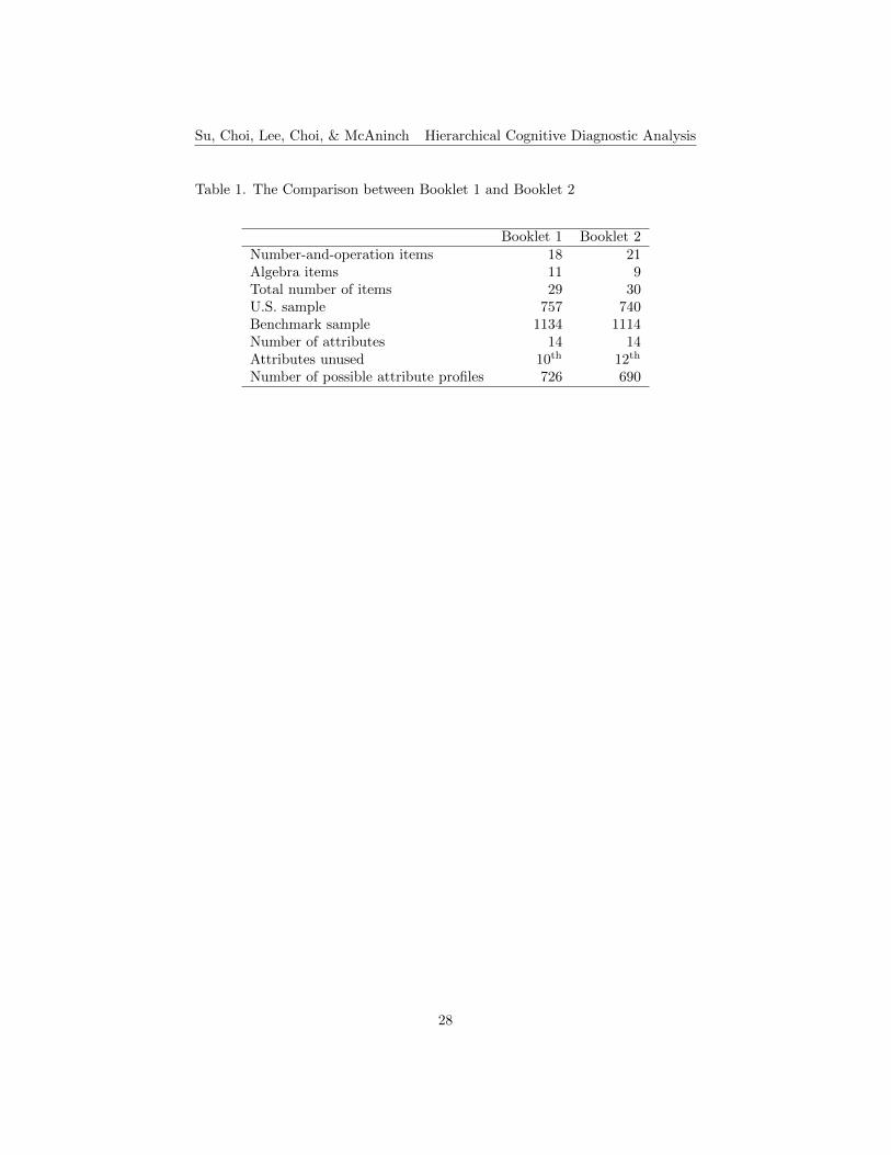
Su, Choi, Lee, Choi, & McAninch Hierarchical Cognitive Diagnostic Analysis
Table 1. The Comparison between Booklet 1 and Booklet 2
Booklet 1 Booklet 2Number-and-operation items 18 21Algebra items 11 9Total number of items 29 30U.S. sample 757 740Benchmark sample 1134 1114Number of attributes 14 14Attributes unused 10th 12th
Number of possible attribute profiles 726 690
28
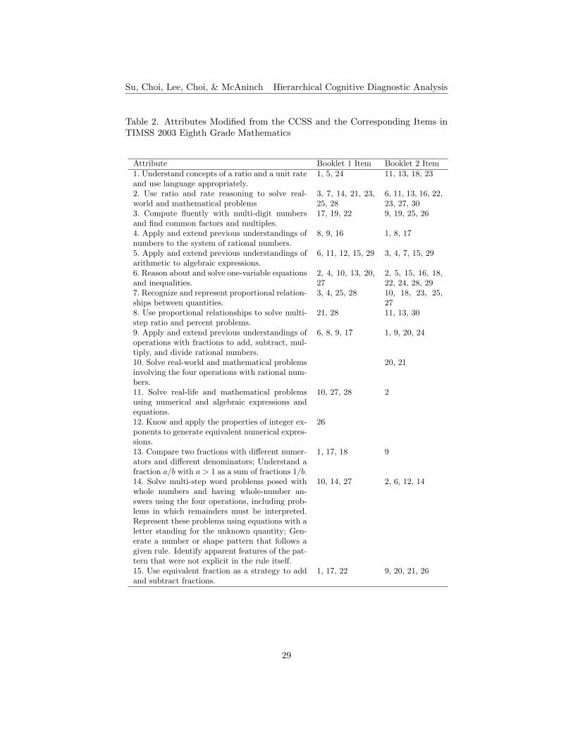
Su, Choi, Lee, Choi, & McAninch Hierarchical Cognitive Diagnostic Analysis
Table 2. Attributes Modified from the CCSS and the Corresponding Items inTIMSS 2003 Eighth Grade Mathematics
Attribute Booklet 1 Item Booklet 2 Item1. Understand concepts of a ratio and a unit rateand use language appropriately.
1, 5, 24 11, 13, 18, 23
2. Use ratio and rate reasoning to solve real-world and mathematical problems
3, 7, 14, 21, 23,25, 28
6, 11, 13, 16, 22,23, 27, 30
3. Compute fluently with multi-digit numbersand find common factors and multiples.
17, 19, 22 9, 19, 25, 26
4. Apply and extend previous understandings ofnumbers to the system of rational numbers.
8, 9, 16 1, 8, 17
5. Apply and extend previous understandings ofarithmetic to algebraic expressions.
6, 11, 12, 15, 29 3, 4, 7, 15, 29
6. Reason about and solve one-variable equationsand inequalities.
2, 4, 10, 13, 20,27
2, 5, 15, 16, 18,22, 24, 28, 29
7. Recognize and represent proportional relation-ships between quantities.
3, 4, 25, 28 10, 18, 23, 25,27
8. Use proportional relationships to solve multi-step ratio and percent problems.
21, 28 11, 13, 30
9. Apply and extend previous understandings ofoperations with fractions to add, subtract, mul-tiply, and divide rational numbers.
6, 8, 9, 17 1, 9, 20, 24
10. Solve real-world and mathematical problemsinvolving the four operations with rational num-bers.
20, 21
11. Solve real-life and mathematical problemsusing numerical and algebraic expressions andequations.
10, 27, 28 2
12. Know and apply the properties of integer ex-ponents to generate equivalent numerical expres-sions.
26
13. Compare two fractions with different numer-ators and different denominators; Understand afraction a/b with a > 1 as a sum of fractions 1/b.
1, 17, 18 9
14. Solve multi-step word problems posed withwhole numbers and having whole-number an-swers using the four operations, including prob-lems in which remainders must be interpreted.Represent these problems using equations with aletter standing for the unknown quantity; Gen-erate a number or shape pattern that follows agiven rule. Identify apparent features of the pat-tern that were not explicit in the rule itself.
10, 14, 27 2, 6, 12, 14
15. Use equivalent fraction as a strategy to addand subtract fractions.
1, 17, 22 9, 20, 21, 26
29
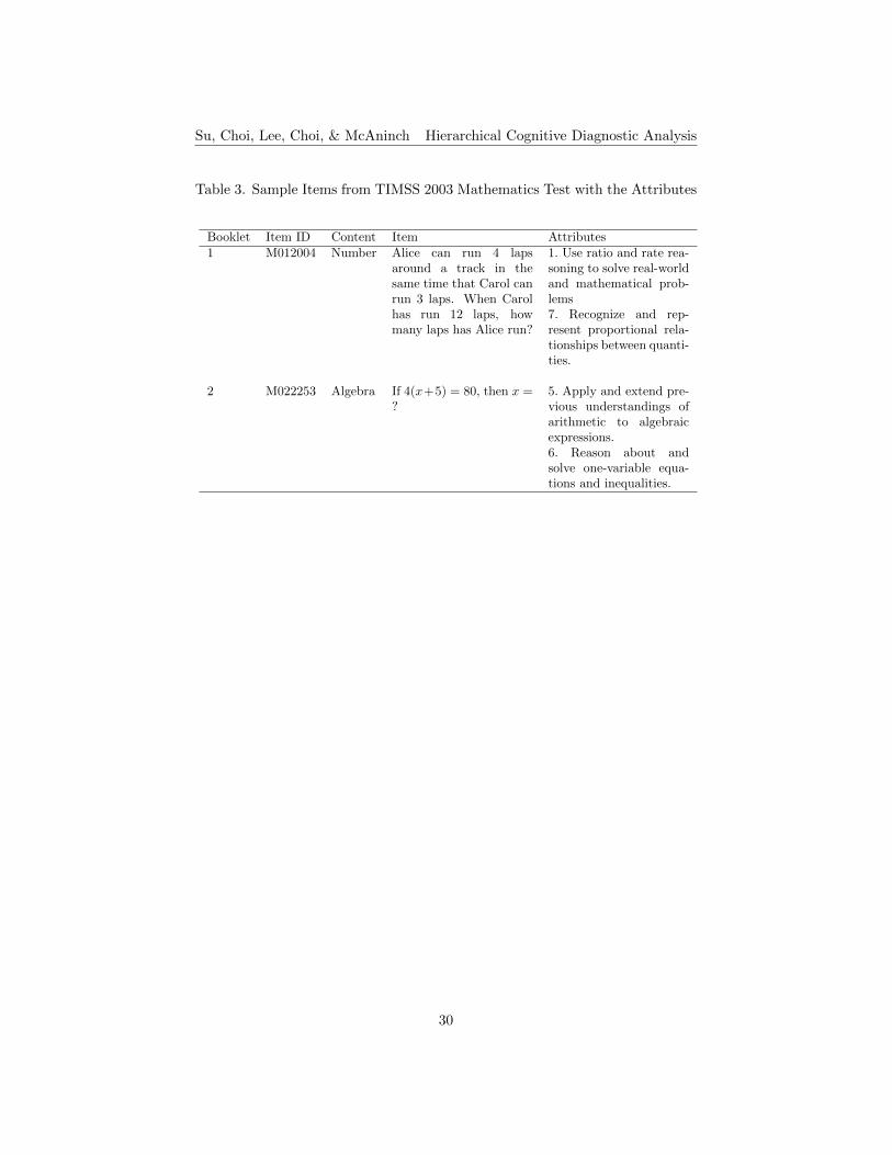
Su, Choi, Lee, Choi, & McAninch Hierarchical Cognitive Diagnostic Analysis
Table 3. Sample Items from TIMSS 2003 Mathematics Test with the Attributes
Booklet Item ID Content Item Attributes1 M012004 Number Alice can run 4 laps 1. Use ratio and rate rea-
around a track in the soning to solve real-worldsame time that Carol can and mathematical prob-run 3 laps. When Carol lemshas run 12 laps, how 7. Recognize and rep-many laps has Alice run? resent proportional rela-
tionships between quanti-ties.
2 M022253 Algebra If 4(x+5) = 80, then x = 5. Apply and extend pre-? vious understandings of
arithmetic to algebraicexpressions.6. Reason about andsolve one-variable equa-tions and inequalities.
30
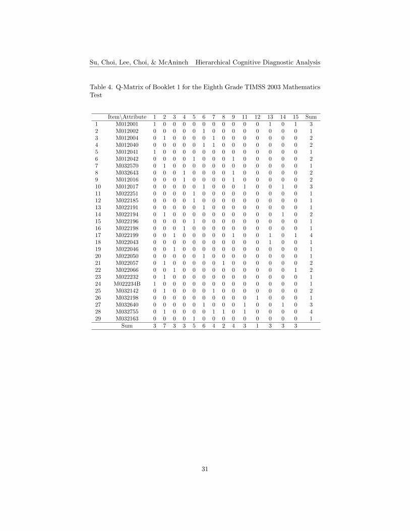
Su, Choi, Lee, Choi, & McAninch Hierarchical Cognitive Diagnostic Analysis
Table 4. Q-Matrix of Booklet 1 for the Eighth Grade TIMSS 2003 MathematicsTest
Item\Attribute 1 2 3 4 5 6 7 8 9 11 12 13 14 15 Sum1 M012001 1 0 0 0 0 0 0 0 0 0 0 1 0 1 32 M012002 0 0 0 0 0 1 0 0 0 0 0 0 0 0 13 M012004 0 1 0 0 0 0 1 0 0 0 0 0 0 0 24 M012040 0 0 0 0 0 1 1 0 0 0 0 0 0 0 25 M012041 1 0 0 0 0 0 0 0 0 0 0 0 0 0 16 M012042 0 0 0 0 1 0 0 0 1 0 0 0 0 0 27 M032570 0 1 0 0 0 0 0 0 0 0 0 0 0 0 18 M032643 0 0 0 1 0 0 0 0 1 0 0 0 0 0 29 M012016 0 0 0 1 0 0 0 0 1 0 0 0 0 0 210 M012017 0 0 0 0 0 1 0 0 0 1 0 0 1 0 311 M022251 0 0 0 0 1 0 0 0 0 0 0 0 0 0 112 M022185 0 0 0 0 1 0 0 0 0 0 0 0 0 0 113 M022191 0 0 0 0 0 1 0 0 0 0 0 0 0 0 114 M022194 0 1 0 0 0 0 0 0 0 0 0 0 1 0 215 M022196 0 0 0 0 1 0 0 0 0 0 0 0 0 0 116 M022198 0 0 0 1 0 0 0 0 0 0 0 0 0 0 117 M022199 0 0 1 0 0 0 0 0 1 0 0 1 0 1 418 M022043 0 0 0 0 0 0 0 0 0 0 0 1 0 0 119 M022046 0 0 1 0 0 0 0 0 0 0 0 0 0 0 120 M022050 0 0 0 0 0 1 0 0 0 0 0 0 0 0 121 M022057 0 1 0 0 0 0 0 1 0 0 0 0 0 0 222 M022066 0 0 1 0 0 0 0 0 0 0 0 0 0 1 223 M022232 0 1 0 0 0 0 0 0 0 0 0 0 0 0 124 M022234B 1 0 0 0 0 0 0 0 0 0 0 0 0 0 125 M032142 0 1 0 0 0 0 1 0 0 0 0 0 0 0 226 M032198 0 0 0 0 0 0 0 0 0 0 1 0 0 0 127 M032640 0 0 0 0 0 1 0 0 0 1 0 0 1 0 328 M032755 0 1 0 0 0 0 1 1 0 1 0 0 0 0 429 M032163 0 0 0 0 1 0 0 0 0 0 0 0 0 0 1
Sum 3 7 3 3 5 6 4 2 4 3 1 3 3 3
31
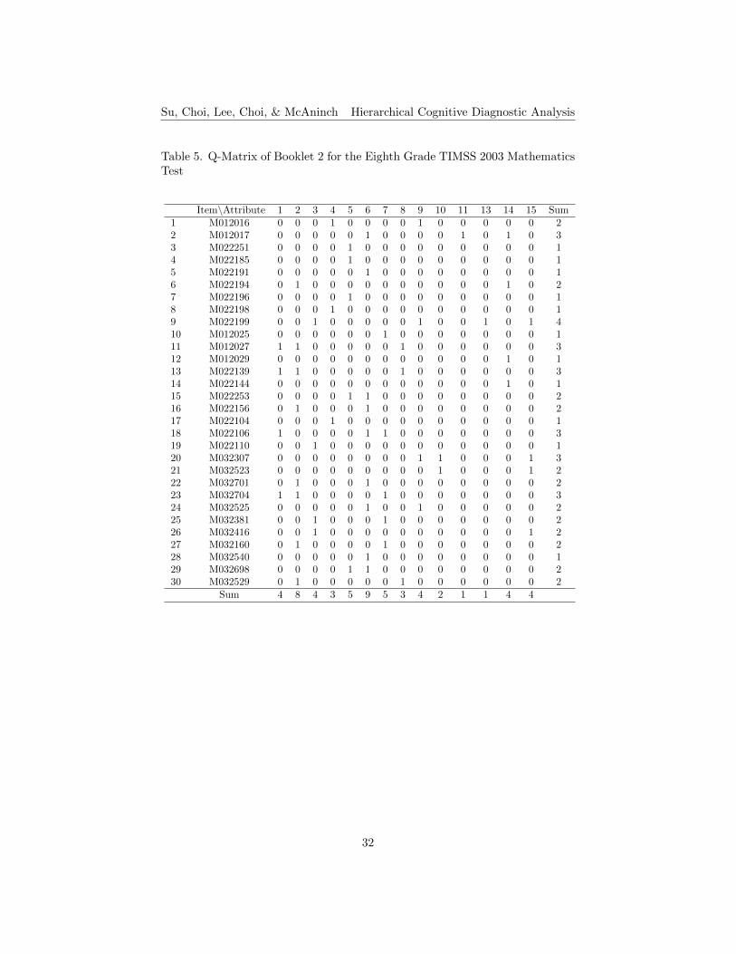
Su, Choi, Lee, Choi, & McAninch Hierarchical Cognitive Diagnostic Analysis
Table 5. Q-Matrix of Booklet 2 for the Eighth Grade TIMSS 2003 MathematicsTest
Item\Attribute 1 2 3 4 5 6 7 8 9 10 11 13 14 15 Sum1 M012016 0 0 0 1 0 0 0 0 1 0 0 0 0 0 22 M012017 0 0 0 0 0 1 0 0 0 0 1 0 1 0 33 M022251 0 0 0 0 1 0 0 0 0 0 0 0 0 0 14 M022185 0 0 0 0 1 0 0 0 0 0 0 0 0 0 15 M022191 0 0 0 0 0 1 0 0 0 0 0 0 0 0 16 M022194 0 1 0 0 0 0 0 0 0 0 0 0 1 0 27 M022196 0 0 0 0 1 0 0 0 0 0 0 0 0 0 18 M022198 0 0 0 1 0 0 0 0 0 0 0 0 0 0 19 M022199 0 0 1 0 0 0 0 0 1 0 0 1 0 1 410 M012025 0 0 0 0 0 0 1 0 0 0 0 0 0 0 111 M012027 1 1 0 0 0 0 0 1 0 0 0 0 0 0 312 M012029 0 0 0 0 0 0 0 0 0 0 0 0 1 0 113 M022139 1 1 0 0 0 0 0 1 0 0 0 0 0 0 314 M022144 0 0 0 0 0 0 0 0 0 0 0 0 1 0 115 M022253 0 0 0 0 1 1 0 0 0 0 0 0 0 0 216 M022156 0 1 0 0 0 1 0 0 0 0 0 0 0 0 217 M022104 0 0 0 1 0 0 0 0 0 0 0 0 0 0 118 M022106 1 0 0 0 0 1 1 0 0 0 0 0 0 0 319 M022110 0 0 1 0 0 0 0 0 0 0 0 0 0 0 120 M032307 0 0 0 0 0 0 0 0 1 1 0 0 0 1 321 M032523 0 0 0 0 0 0 0 0 0 1 0 0 0 1 222 M032701 0 1 0 0 0 1 0 0 0 0 0 0 0 0 223 M032704 1 1 0 0 0 0 1 0 0 0 0 0 0 0 324 M032525 0 0 0 0 0 1 0 0 1 0 0 0 0 0 225 M032381 0 0 1 0 0 0 1 0 0 0 0 0 0 0 226 M032416 0 0 1 0 0 0 0 0 0 0 0 0 0 1 227 M032160 0 1 0 0 0 0 1 0 0 0 0 0 0 0 228 M032540 0 0 0 0 0 1 0 0 0 0 0 0 0 0 129 M032698 0 0 0 0 1 1 0 0 0 0 0 0 0 0 230 M032529 0 1 0 0 0 0 0 1 0 0 0 0 0 0 2
Sum 4 8 4 3 5 9 5 3 4 2 1 1 4 4
32

Su, Choi, Lee, Choi, & McAninch Hierarchical Cognitive Diagnostic Analysis
Table 6. Results of Model Fit Indices for TIMSS Data under the DINA andDINA-H Models
Booklet 1 Booklet 2Model Fit AIC BIC AIC BIC
DINA 55702 131814 56946 132693U.S. Sample DINA-H 24602 28226 25755 29205
Difference 31101 103587 31191 103488DINA 67861 150602 70821 153295
Benchmark Sample DINA-H 36953 40894 39679 43435Difference 30908 109708 31143 109859
33
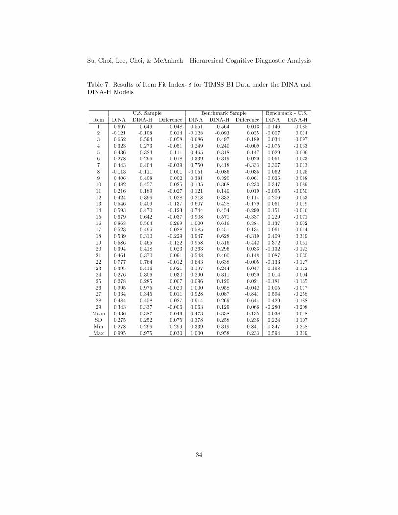
Su, Choi, Lee, Choi, & McAninch Hierarchical Cognitive Diagnostic Analysis
Table 7. Results of Item Fit Index- δ for TIMSS B1 Data under the DINA andDINA-H Models
U.S. Sample Benchmark Sample Benchmark - U.S.Item DINA DINA-H Difference DINA DINA-H Difference DINA DINA-H
1 0.697 0.649 -0.048 0.551 0.564 0.013 -0.146 -0.0852 -0.121 -0.108 0.014 -0.128 -0.093 0.035 -0.007 0.0143 0.652 0.594 -0.058 0.686 0.497 -0.189 0.034 -0.0974 0.323 0.273 -0.051 0.249 0.240 -0.009 -0.075 -0.0335 0.436 0.324 -0.111 0.465 0.318 -0.147 0.029 -0.0066 -0.278 -0.296 -0.018 -0.339 -0.319 0.020 -0.061 -0.0237 0.443 0.404 -0.039 0.750 0.418 -0.333 0.307 0.0138 -0.113 -0.111 0.001 -0.051 -0.086 -0.035 0.062 0.0259 0.406 0.408 0.002 0.381 0.320 -0.061 -0.025 -0.08810 0.482 0.457 -0.025 0.135 0.368 0.233 -0.347 -0.08911 0.216 0.189 -0.027 0.121 0.140 0.019 -0.095 -0.05012 0.424 0.396 -0.028 0.218 0.332 0.114 -0.206 -0.06313 0.546 0.409 -0.137 0.607 0.428 -0.179 0.061 0.01914 0.593 0.470 -0.123 0.744 0.454 -0.290 0.151 -0.01615 0.679 0.642 -0.037 0.908 0.571 -0.337 0.229 -0.07116 0.863 0.564 -0.299 1.000 0.616 -0.384 0.137 0.05217 0.523 0.495 -0.028 0.585 0.451 -0.134 0.061 -0.04418 0.539 0.310 -0.229 0.947 0.628 -0.319 0.409 0.31919 0.586 0.465 -0.122 0.958 0.516 -0.442 0.372 0.05120 0.394 0.418 0.023 0.263 0.296 0.033 -0.132 -0.12221 0.461 0.370 -0.091 0.548 0.400 -0.148 0.087 0.03022 0.777 0.764 -0.012 0.643 0.638 -0.005 -0.133 -0.12723 0.395 0.416 0.021 0.197 0.244 0.047 -0.198 -0.17224 0.276 0.306 0.030 0.290 0.311 0.020 0.014 0.00425 0.278 0.285 0.007 0.096 0.120 0.024 -0.181 -0.16526 0.995 0.975 -0.020 1.000 0.958 -0.042 0.005 -0.01727 0.334 0.345 0.011 0.928 0.087 -0.841 0.594 -0.25828 0.484 0.458 -0.027 0.914 0.269 -0.644 0.429 -0.18829 0.343 0.337 -0.006 0.063 0.129 0.066 -0.280 -0.208
Mean 0.436 0.387 -0.049 0.473 0.338 -0.135 0.038 -0.048SD 0.275 0.252 0.075 0.378 0.258 0.236 0.224 0.107Min -0.278 -0.296 -0.299 -0.339 -0.319 -0.841 -0.347 -0.258Max 0.995 0.975 0.030 1.000 0.958 0.233 0.594 0.319
34
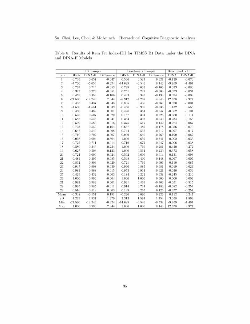
Su, Choi, Lee, Choi, & McAninch Hierarchical Cognitive Diagnostic Analysis
Table 8. Results of Item Fit Index-IDI for TIMSS B1 Data under the DINAand DINA-H Models
U.S. Sample Benchmark Sample Benchmark - U.S.Item DINA DINA-H Difference DINA DINA-H Difference DINA DINA-H
1 0.705 0.657 -0.047 0.566 0.587 0.021 -0.139 -0.0702 -4.730 -5.054 -0.324 -14.689 -6.546 8.143 -9.959 -1.4913 0.767 0.714 -0.053 0.799 0.633 -0.166 0.033 -0.0804 0.323 0.273 -0.051 0.251 0.242 -0.008 -0.073 -0.0315 0.459 0.353 -0.106 0.483 0.345 -0.138 0.024 -0.0086 -21.590 -14.246 7.344 -8.912 -4.269 4.643 12.678 9.9777 0.485 0.437 -0.048 0.805 0.436 -0.369 0.320 -0.0018 -1.590 -1.551 0.039 -0.458 -0.996 -0.538 1.132 0.5559 0.480 0.482 0.001 0.428 0.381 -0.047 -0.052 -0.10110 0.528 0.507 -0.020 0.167 0.394 0.226 -0.360 -0.11411 0.587 0.546 -0.041 0.354 0.393 0.040 -0.234 -0.15312 0.599 0.583 -0.016 0.375 0.517 0.142 -0.224 -0.06713 0.723 0.559 -0.164 0.667 0.489 -0.178 -0.056 -0.07014 0.647 0.549 -0.098 0.744 0.532 -0.212 0.097 -0.01715 0.710 0.702 -0.007 0.909 0.640 -0.269 0.199 -0.06216 0.998 0.694 -0.304 1.000 0.659 -0.341 0.002 -0.03517 0.725 0.711 -0.014 0.719 0.672 -0.047 -0.006 -0.03818 0.580 0.346 -0.234 1.000 0.719 -0.281 0.420 0.37219 0.627 0.503 -0.123 1.000 0.561 -0.439 0.373 0.05820 0.724 0.699 -0.024 0.592 0.606 0.014 -0.131 -0.09321 0.481 0.395 -0.085 0.548 0.400 -0.148 0.067 0.00522 0.832 0.803 -0.029 0.721 0.716 -0.006 -0.110 -0.08723 0.947 0.908 -0.039 0.966 0.885 -0.081 0.019 -0.02324 0.983 0.968 -0.015 0.953 0.931 -0.021 -0.030 -0.03625 0.429 0.432 0.003 0.184 0.222 0.038 -0.245 -0.21026 1.000 0.996 -0.004 1.000 1.000 0.000 0.000 0.00327 0.982 0.983 0.001 0.931 0.469 -0.463 -0.051 -0.51528 0.995 0.985 -0.011 0.914 0.731 -0.183 -0.082 -0.25429 0.516 0.519 0.003 0.139 0.265 0.126 -0.377 -0.254
Mean -0.348 -0.157 0.191 -0.236 0.090 0.326 0.112 0.247SD 4.229 2.937 1.379 3.313 1.591 1.754 3.058 1.899Min -21.590 -14.246 -0.324 -14.689 -6.546 -0.538 -9.959 -1.491Max 1.000 0.996 7.344 1.000 1.000 8.143 12.678 9.977
35

Su, Choi, Lee, Choi, & McAninch Hierarchical Cognitive Diagnostic Analysis
Table 9. Results of Item Fit Index- δ for TIMSS B2 Data under the DINA andDINA-H Models
U.S. Sample Benchmark Sample Benchmark - U.S.Item DINA DINA-H Difference DINA DINA-H Difference DINA DINA-H
1 0.415 0.394 -0.022 0.335 0.320 -0.015 -0.081 -0.0742 0.683 0.643 -0.041 0.492 0.375 -0.117 -0.191 -0.2683 0.121 0.099 -0.021 0.074 0.049 -0.026 -0.046 -0.0514 0.343 0.307 -0.036 0.313 0.296 -0.017 -0.030 -0.0115 0.366 0.329 -0.036 0.330 0.290 -0.040 -0.036 -0.0406 0.363 0.364 0.001 0.429 0.425 -0.004 0.066 0.0617 0.679 0.596 -0.083 0.509 0.443 -0.066 -0.170 -0.1538 0.308 0.337 0.028 0.307 0.336 0.029 -0.002 -0.0019 0.815 0.478 -0.337 0.743 0.497 -0.246 -0.072 0.02010 0.391 0.303 -0.087 0.257 0.194 -0.063 -0.133 -0.10911 0.472 0.488 0.016 0.493 0.545 0.052 0.021 0.05712 0.562 0.527 -0.035 0.430 0.409 -0.021 -0.132 -0.11813 -0.031 -0.030 0.002 -0.027 -0.018 0.008 0.005 0.01114 0.546 0.533 -0.013 0.491 0.444 -0.047 -0.055 -0.08915 0.576 0.557 -0.019 0.517 0.492 -0.025 -0.059 -0.06516 0.808 0.660 -0.147 0.690 0.594 -0.096 -0.117 -0.06617 0.440 0.385 -0.056 0.504 0.412 -0.092 0.064 0.02718 0.440 0.371 -0.069 0.573 0.449 -0.124 0.133 0.07819 0.269 0.261 -0.008 0.107 0.283 0.176 -0.162 0.02220 0.703 0.669 -0.034 0.813 0.746 -0.067 0.110 0.07721 0.411 0.361 -0.050 0.397 0.360 -0.036 -0.015 -0.00122 0.166 0.168 0.002 0.123 0.118 -0.006 -0.043 -0.05123 0.485 0.497 0.012 0.318 0.386 0.068 -0.167 -0.11224 0.606 0.547 -0.059 0.335 0.311 -0.024 -0.271 -0.23625 0.735 0.640 -0.095 0.542 0.293 -0.249 -0.192 -0.34726 0.480 0.462 -0.018 0.476 0.217 -0.259 -0.004 -0.24627 0.230 0.210 -0.019 0.300 0.159 -0.141 0.070 -0.05228 0.230 0.194 -0.036 0.148 0.129 -0.019 -0.082 -0.06529 0.471 0.452 -0.018 0.018 0.018 0.000 -0.453 -0.43430 0.619 0.350 -0.270 0.417 0.158 -0.259 -0.202 -0.192
Mean 0.457 0.405 -0.052 0.382 0.324 -0.058 -0.075 -0.081SD 0.204 0.173 0.078 0.204 0.175 0.099 0.122 0.125Min -0.031 -0.030 -0.337 -0.027 -0.018 -0.259 -0.453 -0.434Max 0.815 0.669 0.028 0.813 0.746 0.176 0.133 0.078
36

Su, Choi, Lee, Choi, & McAninch Hierarchical Cognitive Diagnostic Analysis
Table 10. Results of Item Fit Index-IDI for TIMSS B2 Data under the DINAand DINA-H Models
U.S. Sample Benchmark Sample Benchmark - U.S.Item DINA DINA-H Difference DINA DINA-H Difference DINA DINA-H
1 0.560 0.532 -0.028 0.453 0.434 -0.018 -0.107 -0.0982 0.686 0.654 -0.032 0.498 0.420 -0.079 -0.188 -0.2353 0.386 0.326 -0.060 0.219 0.149 -0.070 -0.167 -0.1774 0.522 0.474 -0.048 0.476 0.461 -0.015 -0.046 -0.0135 0.557 0.488 -0.070 0.401 0.348 -0.053 -0.156 -0.1406 0.473 0.477 0.005 0.490 0.512 0.022 0.018 0.0357 0.744 0.671 -0.073 0.550 0.501 -0.050 -0.193 -0.1708 0.493 0.509 0.016 0.459 0.481 0.022 -0.034 -0.0289 0.822 0.724 -0.098 0.754 0.693 -0.061 -0.068 -0.03110 0.414 0.323 -0.091 0.305 0.226 -0.079 -0.109 -0.09711 0.504 0.519 0.015 0.518 0.567 0.049 0.014 0.04812 0.640 0.605 -0.035 0.522 0.528 0.007 -0.118 -0.07713 -0.385 -0.360 0.025 -0.396 -0.248 0.147 -0.011 0.11214 0.623 0.607 -0.016 0.587 0.577 -0.011 -0.036 -0.03115 0.710 0.698 -0.013 0.640 0.635 -0.005 -0.070 -0.06316 0.952 0.831 -0.121 0.841 0.746 -0.095 -0.111 -0.08517 0.448 0.391 -0.057 0.509 0.419 -0.090 0.061 0.02918 0.776 0.732 -0.044 0.898 0.820 -0.078 0.122 0.08819 0.280 0.270 -0.009 0.127 0.312 0.185 -0.153 0.04120 0.944 0.936 -0.008 0.938 0.889 -0.049 -0.006 -0.04721 0.701 0.631 -0.070 0.811 0.714 -0.097 0.110 0.08322 0.171 0.172 0.001 0.124 0.118 -0.006 -0.047 -0.05423 0.502 0.535 0.033 0.325 0.406 0.081 -0.177 -0.12924 0.658 0.599 -0.060 0.409 0.380 -0.029 -0.249 -0.21825 0.825 0.725 -0.100 0.675 0.404 -0.270 -0.150 -0.32126 0.994 0.975 -0.019 0.987 0.543 -0.444 -0.007 -0.43227 0.721 0.682 -0.039 0.926 0.573 -0.353 0.204 -0.11028 0.320 0.267 -0.052 0.220 0.191 -0.029 -0.099 -0.07729 0.786 0.771 -0.016 0.043 0.043 0.000 -0.743 -0.72830 0.896 0.562 -0.334 0.723 0.324 -0.399 -0.172 -0.238
Mean 0.591 0.544 -0.047 0.501 0.439 -0.062 -0.090 -0.105SD 0.276 0.256 0.067 0.305 0.240 0.140 0.161 0.170Min -0.385 -0.360 -0.334 -0.396 -0.248 -0.444 -0.743 -0.728Max 0.994 0.975 0.033 0.987 0.889 0.185 0.204 0.112
37
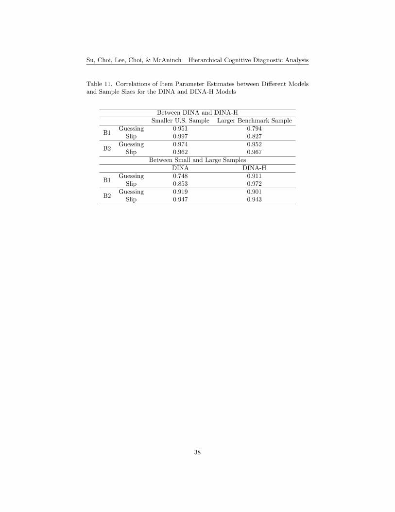
Su, Choi, Lee, Choi, & McAninch Hierarchical Cognitive Diagnostic Analysis
Table 11. Correlations of Item Parameter Estimates between Different Modelsand Sample Sizes for the DINA and DINA-H Models
Between DINA and DINA-HSmaller U.S. Sample Larger Benchmark Sample
B1Guessing 0.951 0.794
Slip 0.997 0.827
B2Guessing 0.974 0.952
Slip 0.962 0.967Between Small and Large Samples
DINA DINA-H
B1Guessing 0.748 0.911
Slip 0.853 0.972
B2Guessing 0.919 0.901
Slip 0.947 0.943
38
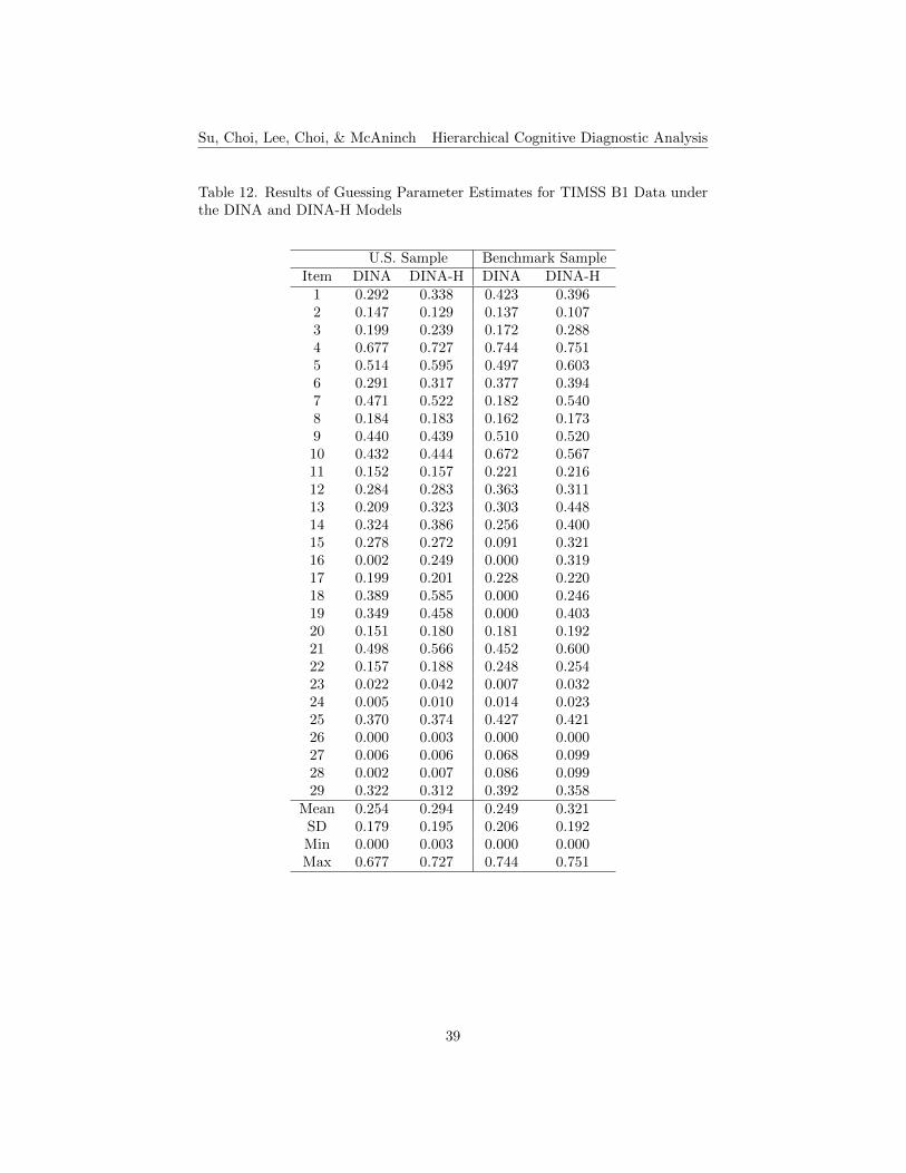
Su, Choi, Lee, Choi, & McAninch Hierarchical Cognitive Diagnostic Analysis
Table 12. Results of Guessing Parameter Estimates for TIMSS B1 Data underthe DINA and DINA-H Models
U.S. Sample Benchmark SampleItem DINA DINA-H DINA DINA-H
1 0.292 0.338 0.423 0.3962 0.147 0.129 0.137 0.1073 0.199 0.239 0.172 0.2884 0.677 0.727 0.744 0.7515 0.514 0.595 0.497 0.6036 0.291 0.317 0.377 0.3947 0.471 0.522 0.182 0.5408 0.184 0.183 0.162 0.1739 0.440 0.439 0.510 0.52010 0.432 0.444 0.672 0.56711 0.152 0.157 0.221 0.21612 0.284 0.283 0.363 0.31113 0.209 0.323 0.303 0.44814 0.324 0.386 0.256 0.40015 0.278 0.272 0.091 0.32116 0.002 0.249 0.000 0.31917 0.199 0.201 0.228 0.22018 0.389 0.585 0.000 0.24619 0.349 0.458 0.000 0.40320 0.151 0.180 0.181 0.19221 0.498 0.566 0.452 0.60022 0.157 0.188 0.248 0.25423 0.022 0.042 0.007 0.03224 0.005 0.010 0.014 0.02325 0.370 0.374 0.427 0.42126 0.000 0.003 0.000 0.00027 0.006 0.006 0.068 0.09928 0.002 0.007 0.086 0.09929 0.322 0.312 0.392 0.358
Mean 0.254 0.294 0.249 0.321SD 0.179 0.195 0.206 0.192Min 0.000 0.003 0.000 0.000Max 0.677 0.727 0.744 0.751
39
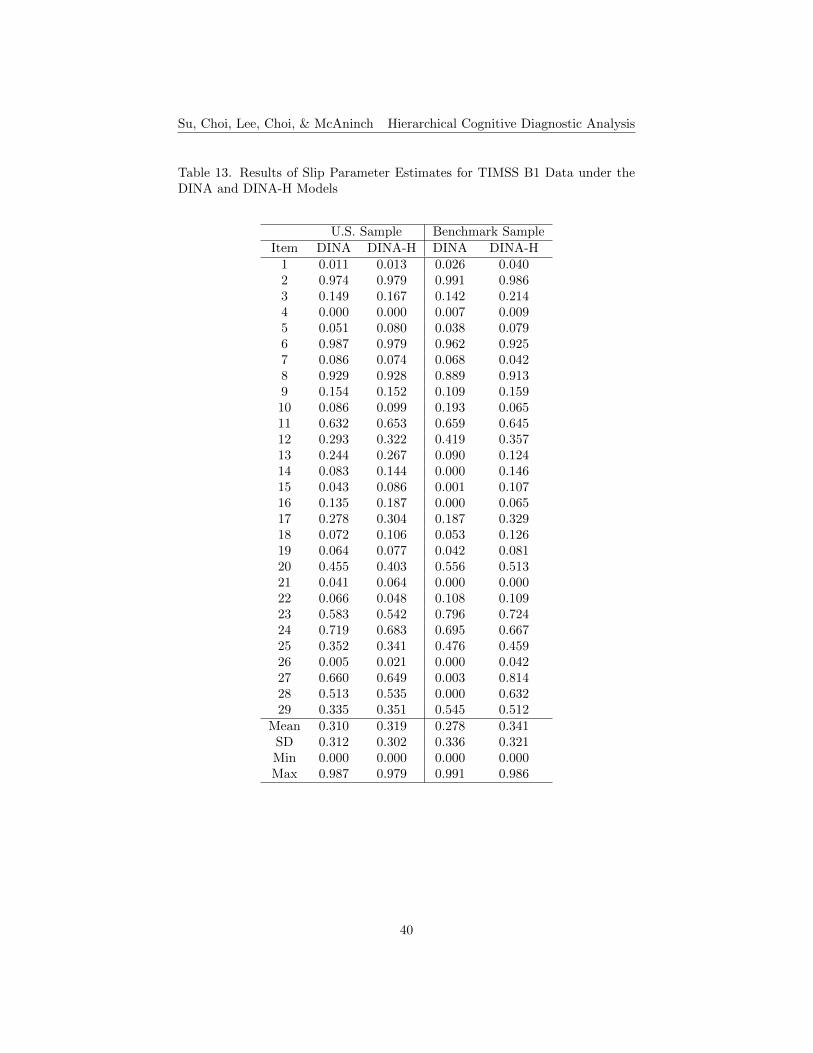
Su, Choi, Lee, Choi, & McAninch Hierarchical Cognitive Diagnostic Analysis
Table 13. Results of Slip Parameter Estimates for TIMSS B1 Data under theDINA and DINA-H Models
U.S. Sample Benchmark SampleItem DINA DINA-H DINA DINA-H
1 0.011 0.013 0.026 0.0402 0.974 0.979 0.991 0.9863 0.149 0.167 0.142 0.2144 0.000 0.000 0.007 0.0095 0.051 0.080 0.038 0.0796 0.987 0.979 0.962 0.9257 0.086 0.074 0.068 0.0428 0.929 0.928 0.889 0.9139 0.154 0.152 0.109 0.15910 0.086 0.099 0.193 0.06511 0.632 0.653 0.659 0.64512 0.293 0.322 0.419 0.35713 0.244 0.267 0.090 0.12414 0.083 0.144 0.000 0.14615 0.043 0.086 0.001 0.10716 0.135 0.187 0.000 0.06517 0.278 0.304 0.187 0.32918 0.072 0.106 0.053 0.12619 0.064 0.077 0.042 0.08120 0.455 0.403 0.556 0.51321 0.041 0.064 0.000 0.00022 0.066 0.048 0.108 0.10923 0.583 0.542 0.796 0.72424 0.719 0.683 0.695 0.66725 0.352 0.341 0.476 0.45926 0.005 0.021 0.000 0.04227 0.660 0.649 0.003 0.81428 0.513 0.535 0.000 0.63229 0.335 0.351 0.545 0.512
Mean 0.310 0.319 0.278 0.341SD 0.312 0.302 0.336 0.321Min 0.000 0.000 0.000 0.000Max 0.987 0.979 0.991 0.986
40
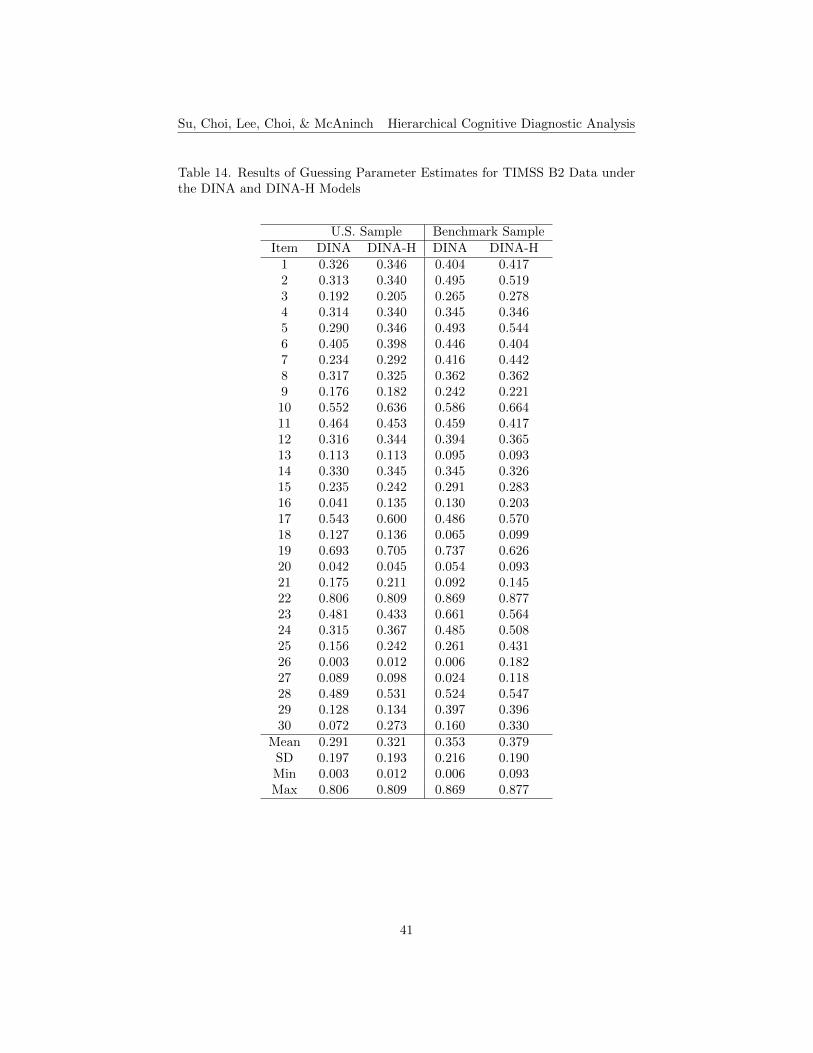
Su, Choi, Lee, Choi, & McAninch Hierarchical Cognitive Diagnostic Analysis
Table 14. Results of Guessing Parameter Estimates for TIMSS B2 Data underthe DINA and DINA-H Models
U.S. Sample Benchmark SampleItem DINA DINA-H DINA DINA-H
1 0.326 0.346 0.404 0.4172 0.313 0.340 0.495 0.5193 0.192 0.205 0.265 0.2784 0.314 0.340 0.345 0.3465 0.290 0.346 0.493 0.5446 0.405 0.398 0.446 0.4047 0.234 0.292 0.416 0.4428 0.317 0.325 0.362 0.3629 0.176 0.182 0.242 0.22110 0.552 0.636 0.586 0.66411 0.464 0.453 0.459 0.41712 0.316 0.344 0.394 0.36513 0.113 0.113 0.095 0.09314 0.330 0.345 0.345 0.32615 0.235 0.242 0.291 0.28316 0.041 0.135 0.130 0.20317 0.543 0.600 0.486 0.57018 0.127 0.136 0.065 0.09919 0.693 0.705 0.737 0.62620 0.042 0.045 0.054 0.09321 0.175 0.211 0.092 0.14522 0.806 0.809 0.869 0.87723 0.481 0.433 0.661 0.56424 0.315 0.367 0.485 0.50825 0.156 0.242 0.261 0.43126 0.003 0.012 0.006 0.18227 0.089 0.098 0.024 0.11828 0.489 0.531 0.524 0.54729 0.128 0.134 0.397 0.39630 0.072 0.273 0.160 0.330
Mean 0.291 0.321 0.353 0.379SD 0.197 0.193 0.216 0.190Min 0.003 0.012 0.006 0.093Max 0.806 0.809 0.869 0.877
41
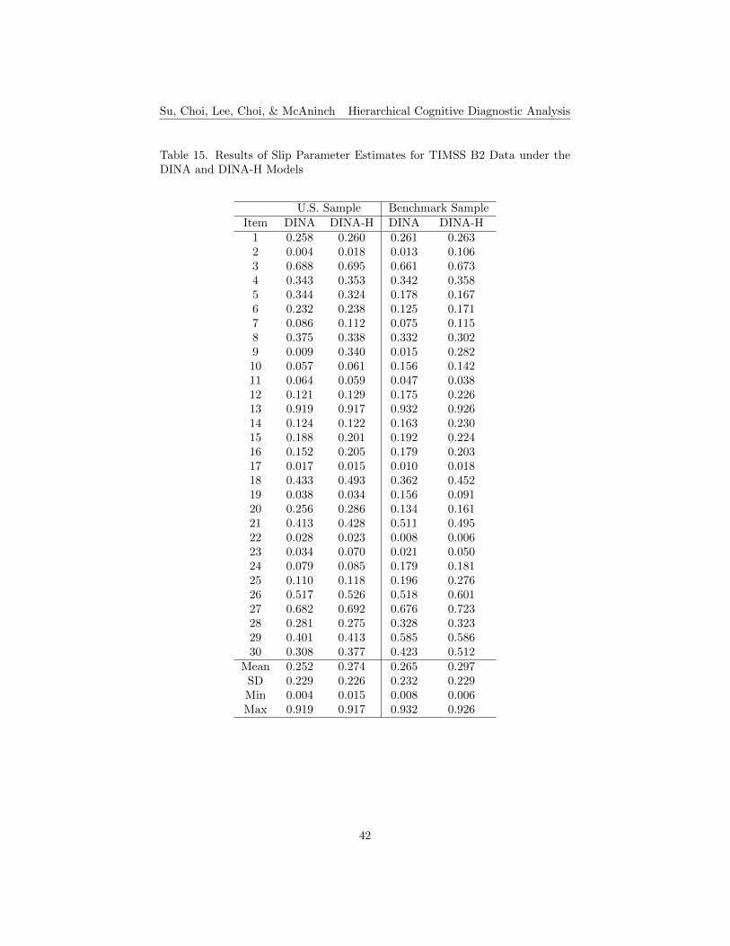
Su, Choi, Lee, Choi, & McAninch Hierarchical Cognitive Diagnostic Analysis
Table 15. Results of Slip Parameter Estimates for TIMSS B2 Data under theDINA and DINA-H Models
U.S. Sample Benchmark SampleItem DINA DINA-H DINA DINA-H
1 0.258 0.260 0.261 0.2632 0.004 0.018 0.013 0.1063 0.688 0.695 0.661 0.6734 0.343 0.353 0.342 0.3585 0.344 0.324 0.178 0.1676 0.232 0.238 0.125 0.1717 0.086 0.112 0.075 0.1158 0.375 0.338 0.332 0.3029 0.009 0.340 0.015 0.28210 0.057 0.061 0.156 0.14211 0.064 0.059 0.047 0.03812 0.121 0.129 0.175 0.22613 0.919 0.917 0.932 0.92614 0.124 0.122 0.163 0.23015 0.188 0.201 0.192 0.22416 0.152 0.205 0.179 0.20317 0.017 0.015 0.010 0.01818 0.433 0.493 0.362 0.45219 0.038 0.034 0.156 0.09120 0.256 0.286 0.134 0.16121 0.413 0.428 0.511 0.49522 0.028 0.023 0.008 0.00623 0.034 0.070 0.021 0.05024 0.079 0.085 0.179 0.18125 0.110 0.118 0.196 0.27626 0.517 0.526 0.518 0.60127 0.682 0.692 0.676 0.72328 0.281 0.275 0.328 0.32329 0.401 0.413 0.585 0.58630 0.308 0.377 0.423 0.512
Mean 0.252 0.274 0.265 0.297SD 0.229 0.226 0.232 0.229Min 0.004 0.015 0.008 0.006Max 0.919 0.917 0.932 0.926
42
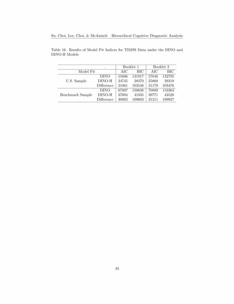
Su, Choi, Lee, Choi, & McAninch Hierarchical Cognitive Diagnostic Analysis
Table 16. Results of Model Fit Indices for TIMSS Data under the DINO andDINO-H Models
. Booklet 1 Booklet 2Model Fit AIC BIC AIC BIC
DINO 55806 131917 57048 132795U.S. Sample DINO-H 24745 28370 25868 29319
Difference 31061 103548 31179 103476DINO 67897 150638 70889 153363
Benchmark Sample DINO-H 37094 41035 39771 43528Difference 30802 109603 31211 109927
43
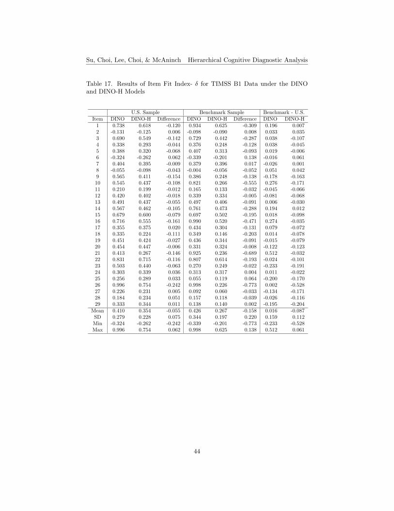
Su, Choi, Lee, Choi, & McAninch Hierarchical Cognitive Diagnostic Analysis
Table 17. Results of Item Fit Index- δ for TIMSS B1 Data under the DINOand DINO-H Models
U.S. Sample Benchmark Sample Benchmark - U.S.Item DINO DINO-H Difference DINO DINO-H Difference DINO DINO-H
1 0.738 0.618 -0.120 0.934 0.625 -0.309 0.196 0.0072 -0.131 -0.125 0.006 -0.098 -0.090 0.008 0.033 0.0353 0.690 0.549 -0.142 0.729 0.442 -0.287 0.038 -0.1074 0.338 0.293 -0.044 0.376 0.248 -0.128 0.038 -0.0455 0.388 0.320 -0.068 0.407 0.313 -0.093 0.019 -0.0066 -0.324 -0.262 0.062 -0.339 -0.201 0.138 -0.016 0.0617 0.404 0.395 -0.009 0.379 0.396 0.017 -0.026 0.0018 -0.055 -0.098 -0.043 -0.004 -0.056 -0.052 0.051 0.0429 0.565 0.411 -0.154 0.386 0.248 -0.138 -0.178 -0.16310 0.545 0.437 -0.108 0.821 0.266 -0.555 0.276 -0.17111 0.210 0.199 -0.012 0.165 0.133 -0.032 -0.045 -0.06612 0.420 0.402 -0.018 0.339 0.334 -0.005 -0.081 -0.06813 0.491 0.437 -0.055 0.497 0.406 -0.091 0.006 -0.03014 0.567 0.462 -0.105 0.761 0.473 -0.288 0.194 0.01215 0.679 0.600 -0.079 0.697 0.502 -0.195 0.018 -0.09816 0.716 0.555 -0.161 0.990 0.520 -0.471 0.274 -0.03517 0.355 0.375 0.020 0.434 0.304 -0.131 0.079 -0.07218 0.335 0.224 -0.111 0.349 0.146 -0.203 0.014 -0.07819 0.451 0.424 -0.027 0.436 0.344 -0.091 -0.015 -0.07920 0.454 0.447 -0.006 0.331 0.324 -0.008 -0.122 -0.12321 0.413 0.267 -0.146 0.925 0.236 -0.689 0.512 -0.03222 0.831 0.715 -0.116 0.807 0.614 -0.193 -0.024 -0.10123 0.503 0.440 -0.063 0.270 0.249 -0.022 -0.233 -0.19124 0.303 0.339 0.036 0.313 0.317 0.004 0.011 -0.02225 0.256 0.289 0.033 0.055 0.119 0.064 -0.200 -0.17026 0.996 0.754 -0.242 0.998 0.226 -0.773 0.002 -0.52827 0.226 0.231 0.005 0.092 0.060 -0.033 -0.134 -0.17128 0.184 0.234 0.051 0.157 0.118 -0.039 -0.026 -0.11629 0.333 0.344 0.011 0.138 0.140 0.002 -0.195 -0.204
Mean 0.410 0.354 -0.055 0.426 0.267 -0.158 0.016 -0.087SD 0.279 0.228 0.075 0.344 0.197 0.220 0.159 0.112Min -0.324 -0.262 -0.242 -0.339 -0.201 -0.773 -0.233 -0.528Max 0.996 0.754 0.062 0.998 0.625 0.138 0.512 0.061
44
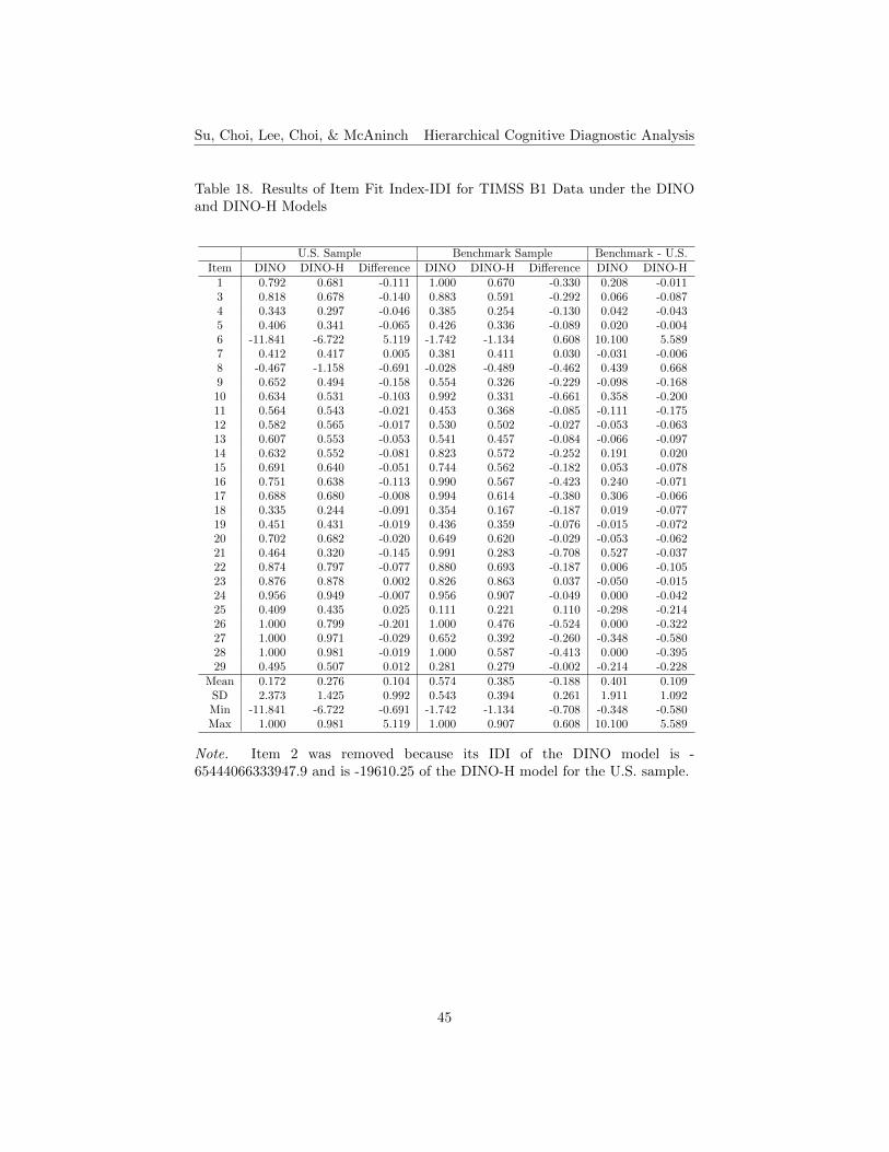
Su, Choi, Lee, Choi, & McAninch Hierarchical Cognitive Diagnostic Analysis
Table 18. Results of Item Fit Index-IDI for TIMSS B1 Data under the DINOand DINO-H Models
U.S. Sample Benchmark Sample Benchmark - U.S.Item DINO DINO-H Difference DINO DINO-H Difference DINO DINO-H
1 0.792 0.681 -0.111 1.000 0.670 -0.330 0.208 -0.0113 0.818 0.678 -0.140 0.883 0.591 -0.292 0.066 -0.0874 0.343 0.297 -0.046 0.385 0.254 -0.130 0.042 -0.0435 0.406 0.341 -0.065 0.426 0.336 -0.089 0.020 -0.0046 -11.841 -6.722 5.119 -1.742 -1.134 0.608 10.100 5.5897 0.412 0.417 0.005 0.381 0.411 0.030 -0.031 -0.0068 -0.467 -1.158 -0.691 -0.028 -0.489 -0.462 0.439 0.6689 0.652 0.494 -0.158 0.554 0.326 -0.229 -0.098 -0.16810 0.634 0.531 -0.103 0.992 0.331 -0.661 0.358 -0.20011 0.564 0.543 -0.021 0.453 0.368 -0.085 -0.111 -0.17512 0.582 0.565 -0.017 0.530 0.502 -0.027 -0.053 -0.06313 0.607 0.553 -0.053 0.541 0.457 -0.084 -0.066 -0.09714 0.632 0.552 -0.081 0.823 0.572 -0.252 0.191 0.02015 0.691 0.640 -0.051 0.744 0.562 -0.182 0.053 -0.07816 0.751 0.638 -0.113 0.990 0.567 -0.423 0.240 -0.07117 0.688 0.680 -0.008 0.994 0.614 -0.380 0.306 -0.06618 0.335 0.244 -0.091 0.354 0.167 -0.187 0.019 -0.07719 0.451 0.431 -0.019 0.436 0.359 -0.076 -0.015 -0.07220 0.702 0.682 -0.020 0.649 0.620 -0.029 -0.053 -0.06221 0.464 0.320 -0.145 0.991 0.283 -0.708 0.527 -0.03722 0.874 0.797 -0.077 0.880 0.693 -0.187 0.006 -0.10523 0.876 0.878 0.002 0.826 0.863 0.037 -0.050 -0.01524 0.956 0.949 -0.007 0.956 0.907 -0.049 0.000 -0.04225 0.409 0.435 0.025 0.111 0.221 0.110 -0.298 -0.21426 1.000 0.799 -0.201 1.000 0.476 -0.524 0.000 -0.32227 1.000 0.971 -0.029 0.652 0.392 -0.260 -0.348 -0.58028 1.000 0.981 -0.019 1.000 0.587 -0.413 0.000 -0.39529 0.495 0.507 0.012 0.281 0.279 -0.002 -0.214 -0.228
Mean 0.172 0.276 0.104 0.574 0.385 -0.188 0.401 0.109SD 2.373 1.425 0.992 0.543 0.394 0.261 1.911 1.092Min -11.841 -6.722 -0.691 -1.742 -1.134 -0.708 -0.348 -0.580Max 1.000 0.981 5.119 1.000 0.907 0.608 10.100 5.589
Note. Item 2 was removed because its IDI of the DINO model is -65444066333947.9 and is -19610.25 of the DINO-H model for the U.S. sample.
45

Su, Choi, Lee, Choi, & McAninch Hierarchical Cognitive Diagnostic Analysis
Table 19. Results of Item Fit Index- δ for TIMSS B2 Data under the DINOand DINO-H Models
U.S. Sample Benchmark Sample Benchmark - U.S.Item DINO DINO-H Difference DINO DINO-H Difference DINO DINO-H
1 0.381 0.344 -0.038 0.293 0.288 -0.005 -0.088 -0.0562 0.708 0.355 -0.353 0.755 0.244 -0.511 0.047 -0.1113 0.096 0.099 0.003 0.073 0.055 -0.018 -0.023 -0.0444 0.345 0.322 -0.023 0.287 0.281 -0.006 -0.058 -0.0415 0.367 0.342 -0.025 0.275 0.296 0.022 -0.092 -0.0466 0.339 0.338 -0.001 0.447 0.392 -0.055 0.108 0.0547 0.647 0.556 -0.091 0.513 0.404 -0.110 -0.134 -0.1528 0.361 0.339 -0.022 0.301 0.291 -0.010 -0.060 -0.0489 0.658 0.582 -0.076 0.542 0.493 -0.049 -0.116 -0.08910 0.298 0.293 -0.004 0.203 0.213 0.010 -0.095 -0.08011 0.552 0.437 -0.115 0.489 0.390 -0.100 -0.063 -0.04812 0.568 0.516 -0.053 0.382 0.382 0.000 -0.186 -0.13413 -0.036 -0.025 0.011 0.001 -0.001 -0.002 0.038 0.02414 0.505 0.494 -0.010 0.455 0.408 -0.047 -0.050 -0.08615 0.564 0.535 -0.029 0.526 0.486 -0.040 -0.038 -0.04916 0.649 0.622 -0.028 0.653 0.583 -0.069 0.003 -0.03817 0.373 0.338 -0.035 0.414 0.328 -0.086 0.041 -0.01018 0.355 0.333 -0.021 0.454 0.427 -0.027 0.100 0.09419 0.129 0.141 0.012 0.054 0.174 0.119 -0.075 0.03320 0.671 0.598 -0.073 0.759 0.664 -0.095 0.088 0.06621 0.468 0.436 -0.032 0.438 0.467 0.029 -0.030 0.03122 0.199 0.185 -0.015 0.131 0.126 -0.005 -0.069 -0.05923 0.553 0.486 -0.067 0.377 0.333 -0.044 -0.177 -0.15324 0.533 0.510 -0.023 0.338 0.304 -0.034 -0.195 -0.20625 0.705 0.619 -0.086 0.567 0.300 -0.267 -0.137 -0.31926 0.487 0.328 -0.160 0.500 0.189 -0.311 0.013 -0.13827 0.210 0.217 0.007 0.331 0.123 -0.209 0.121 -0.09428 0.221 0.219 -0.002 0.120 0.134 0.014 -0.100 -0.08529 0.452 0.446 -0.006 0.014 0.025 0.011 -0.438 -0.42130 0.481 0.293 -0.189 0.529 0.111 -0.418 0.048 -0.181
Mean 0.428 0.377 -0.051 0.374 0.297 -0.077 -0.054 -0.080SD 0.192 0.161 0.075 0.204 0.163 0.137 0.113 0.108Min -0.036 -0.025 -0.353 0.001 -0.001 -0.511 -0.438 -0.421Max 0.708 0.622 0.012 0.759 0.664 0.119 0.121 0.094
46

Su, Choi, Lee, Choi, & McAninch Hierarchical Cognitive Diagnostic Analysis
Table 20. Results of Item Fit Index-IDI for TIMSS B2 Data under the DINOand DINO-H Models
U.S. Sample Benchmark Sample Benchmark - U.S.Item DINO DINO-H Difference DINO DINO-H Difference DINO DINO-H
1 0.537 0.487 -0.050 0.426 0.406 -0.020 -0.111 -0.0822 0.983 0.515 -0.468 0.984 0.327 -0.657 0.001 -0.1883 0.305 0.318 0.014 0.211 0.165 -0.047 -0.093 -0.1544 0.491 0.477 -0.014 0.428 0.428 -0.001 -0.063 -0.0495 0.498 0.474 -0.024 0.326 0.344 0.018 -0.172 -0.1306 0.447 0.454 0.007 0.521 0.489 -0.033 0.075 0.0357 0.657 0.612 -0.045 0.530 0.450 -0.080 -0.127 -0.1638 0.525 0.492 -0.033 0.435 0.409 -0.025 -0.090 -0.0829 1.000 0.975 -0.025 0.999 0.953 -0.046 -0.001 -0.02210 0.315 0.306 -0.008 0.218 0.234 0.015 -0.096 -0.07311 0.606 0.503 -0.103 0.595 0.470 -0.125 -0.012 -0.03312 0.596 0.581 -0.015 0.465 0.482 0.018 -0.131 -0.09813 -0.438 -0.287 0.150 0.017 -0.011 -0.027 0.454 0.27714 0.547 0.561 0.014 0.540 0.518 -0.021 -0.007 -0.04215 0.695 0.663 -0.032 0.691 0.628 -0.063 -0.004 -0.03516 0.816 0.799 -0.017 0.801 0.755 -0.046 -0.015 -0.04417 0.376 0.343 -0.033 0.416 0.334 -0.082 0.040 -0.00918 0.772 0.719 -0.054 0.902 0.835 -0.067 0.130 0.11619 0.131 0.144 0.013 0.064 0.193 0.130 -0.067 0.05020 0.966 0.935 -0.031 0.966 0.886 -0.080 0.000 -0.04921 0.700 0.684 -0.016 0.769 0.775 0.007 0.069 0.09122 0.200 0.187 -0.013 0.131 0.126 -0.005 -0.069 -0.06123 0.595 0.517 -0.078 0.390 0.341 -0.049 -0.205 -0.17624 0.588 0.569 -0.019 0.409 0.372 -0.037 -0.179 -0.19725 0.786 0.721 -0.065 0.620 0.440 -0.180 -0.166 -0.28126 0.852 0.779 -0.073 0.794 0.516 -0.278 -0.058 -0.26327 0.681 0.680 -0.002 0.740 0.439 -0.301 0.059 -0.24128 0.289 0.287 -0.002 0.177 0.194 0.017 -0.112 -0.09329 0.761 0.744 -0.016 0.035 0.060 0.025 -0.725 -0.68530 0.684 0.523 -0.161 0.691 0.248 -0.443 0.007 -0.275
Mean 0.565 0.525 -0.040 0.510 0.427 -0.083 -0.056 -0.099SD 0.292 0.251 0.095 0.287 0.238 0.155 0.177 0.165Min -0.438 -0.287 -0.468 0.017 -0.011 -0.657 -0.725 -0.685Max 1.000 0.975 0.150 0.999 0.953 0.130 0.454 0.277
47
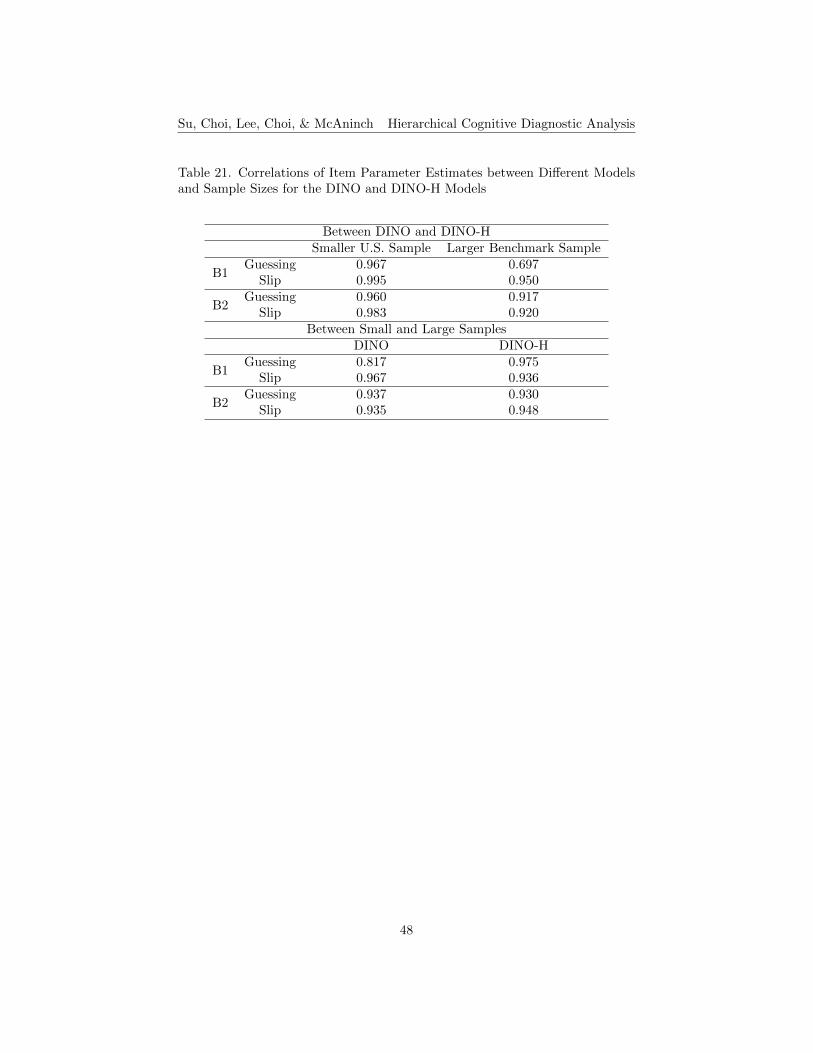
Su, Choi, Lee, Choi, & McAninch Hierarchical Cognitive Diagnostic Analysis
Table 21. Correlations of Item Parameter Estimates between Different Modelsand Sample Sizes for the DINO and DINO-H Models
Between DINO and DINO-HSmaller U.S. Sample Larger Benchmark Sample
B1Guessing 0.967 0.697
Slip 0.995 0.950
B2Guessing 0.960 0.917
Slip 0.983 0.920Between Small and Large Samples
DINO DINO-H
B1Guessing 0.817 0.975
Slip 0.967 0.936
B2Guessing 0.937 0.930
Slip 0.935 0.948
48
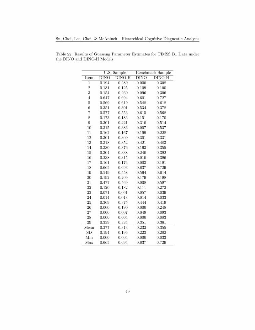
Su, Choi, Lee, Choi, & McAninch Hierarchical Cognitive Diagnostic Analysis
Table 22. Results of Guessing Parameter Estimates for TIMSS B1 Data underthe DINO and DINO-H Models
U.S. Sample Benchmark SampleItem DINO DINO-H DINO DINO-H
1 0.194 0.289 0.000 0.3082 0.131 0.125 0.109 0.1003 0.154 0.260 0.096 0.3064 0.647 0.694 0.601 0.7275 0.569 0.619 0.548 0.6186 0.351 0.301 0.534 0.3787 0.577 0.553 0.615 0.5688 0.173 0.183 0.151 0.1709 0.301 0.421 0.310 0.51410 0.315 0.386 0.007 0.53711 0.162 0.167 0.199 0.22812 0.301 0.309 0.301 0.33113 0.318 0.352 0.421 0.48314 0.330 0.376 0.163 0.35515 0.304 0.338 0.240 0.39216 0.238 0.315 0.010 0.39617 0.161 0.176 0.003 0.19118 0.665 0.693 0.637 0.72919 0.549 0.558 0.564 0.61420 0.192 0.209 0.179 0.19821 0.477 0.569 0.008 0.59722 0.120 0.182 0.111 0.27223 0.071 0.061 0.057 0.03924 0.014 0.018 0.014 0.03325 0.369 0.375 0.444 0.41926 0.000 0.190 0.000 0.24827 0.000 0.007 0.049 0.09328 0.000 0.004 0.000 0.08329 0.339 0.334 0.351 0.361
Mean 0.277 0.313 0.232 0.355SD 0.194 0.196 0.223 0.202Min 0.000 0.004 0.000 0.033Max 0.665 0.694 0.637 0.729
49

Su, Choi, Lee, Choi, & McAninch Hierarchical Cognitive Diagnostic Analysis
Table 23. Results of Slip Parameter Estimates for TIMSS B1 Data under theDINO and DINO-H Models
U.S. Sample Benchmark SampleItem DINO DINO-H DINO DINO-H
1 0.068 0.092 0.066 0.0672 1.000 1.000 0.990 0.9903 0.156 0.191 0.175 0.2524 0.016 0.013 0.023 0.0255 0.043 0.061 0.045 0.0686 0.973 0.961 0.805 0.8237 0.018 0.052 0.006 0.0368 0.882 0.915 0.853 0.8869 0.134 0.168 0.303 0.23810 0.140 0.177 0.172 0.19711 0.627 0.634 0.636 0.63912 0.279 0.289 0.360 0.33513 0.190 0.211 0.081 0.11014 0.103 0.162 0.076 0.17215 0.017 0.062 0.063 0.10616 0.046 0.130 0.000 0.08417 0.484 0.448 0.563 0.50618 0.000 0.083 0.014 0.12519 0.000 0.018 0.000 0.04220 0.354 0.344 0.490 0.47821 0.110 0.163 0.067 0.16722 0.049 0.103 0.082 0.11423 0.426 0.499 0.673 0.71224 0.683 0.642 0.672 0.65125 0.375 0.336 0.501 0.46226 0.004 0.056 0.002 0.52627 0.774 0.762 0.858 0.84728 0.816 0.761 0.843 0.79929 0.328 0.322 0.511 0.499
Mean 0.314 0.333 0.342 0.378SD 0.327 0.307 0.333 0.306Min 0.000 0.013 0.000 0.025Max 1.000 1.000 0.990 0.990
50
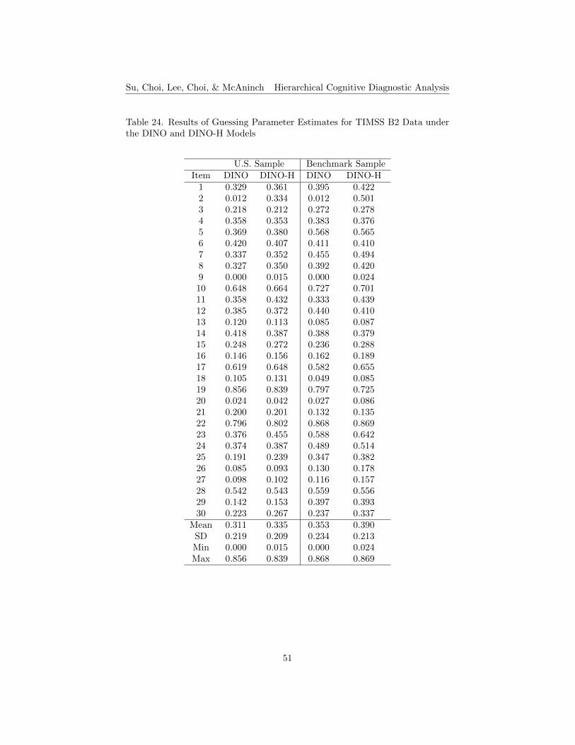
Su, Choi, Lee, Choi, & McAninch Hierarchical Cognitive Diagnostic Analysis
Table 24. Results of Guessing Parameter Estimates for TIMSS B2 Data underthe DINO and DINO-H Models
U.S. Sample Benchmark SampleItem DINO DINO-H DINO DINO-H
1 0.329 0.361 0.395 0.4222 0.012 0.334 0.012 0.5013 0.218 0.212 0.272 0.2784 0.358 0.353 0.383 0.3765 0.369 0.380 0.568 0.5656 0.420 0.407 0.411 0.4107 0.337 0.352 0.455 0.4948 0.327 0.350 0.392 0.4209 0.000 0.015 0.000 0.02410 0.648 0.664 0.727 0.70111 0.358 0.432 0.333 0.43912 0.385 0.372 0.440 0.41013 0.120 0.113 0.085 0.08714 0.418 0.387 0.388 0.37915 0.248 0.272 0.236 0.28816 0.146 0.156 0.162 0.18917 0.619 0.648 0.582 0.65518 0.105 0.131 0.049 0.08519 0.856 0.839 0.797 0.72520 0.024 0.042 0.027 0.08621 0.200 0.201 0.132 0.13522 0.796 0.802 0.868 0.86923 0.376 0.455 0.588 0.64224 0.374 0.387 0.489 0.51425 0.191 0.239 0.347 0.38226 0.085 0.093 0.130 0.17827 0.098 0.102 0.116 0.15728 0.542 0.543 0.559 0.55629 0.142 0.153 0.397 0.39330 0.223 0.267 0.237 0.337
Mean 0.311 0.335 0.353 0.390SD 0.219 0.209 0.234 0.213Min 0.000 0.015 0.000 0.024Max 0.856 0.839 0.868 0.869
51

Su, Choi, Lee, Choi, & McAninch Hierarchical Cognitive Diagnostic Analysis
Table 25. Results of Slip Parameter Estimates for TIMSS B2 Data under theDINO and DINO-H Models
U.S. Sample Benchmark SampleItem DINO DINO-H DINO DINO-H
1 0.290 0.295 0.312 0.2902 0.280 0.311 0.233 0.2553 0.686 0.689 0.655 0.6674 0.297 0.325 0.331 0.3435 0.264 0.279 0.157 0.1396 0.240 0.255 0.142 0.1987 0.016 0.092 0.032 0.1028 0.312 0.311 0.306 0.2899 0.342 0.403 0.457 0.48310 0.054 0.043 0.070 0.08611 0.090 0.131 0.177 0.17112 0.046 0.112 0.178 0.20813 0.917 0.912 0.913 0.91414 0.077 0.118 0.157 0.21315 0.188 0.193 0.238 0.22616 0.204 0.222 0.185 0.22817 0.008 0.014 0.004 0.01718 0.541 0.536 0.496 0.48819 0.016 0.021 0.149 0.10220 0.305 0.360 0.214 0.25121 0.332 0.363 0.431 0.39822 0.005 0.013 0.002 0.00623 0.070 0.059 0.035 0.02524 0.093 0.103 0.173 0.18125 0.104 0.142 0.086 0.31826 0.428 0.579 0.370 0.63327 0.692 0.680 0.553 0.72028 0.237 0.238 0.320 0.31029 0.406 0.401 0.588 0.58230 0.296 0.441 0.234 0.552
Mean 0.261 0.288 0.273 0.313SD 0.223 0.223 0.212 0.226Min 0.005 0.013 0.002 0.006Max 0.917 0.912 0.913 0.914
52
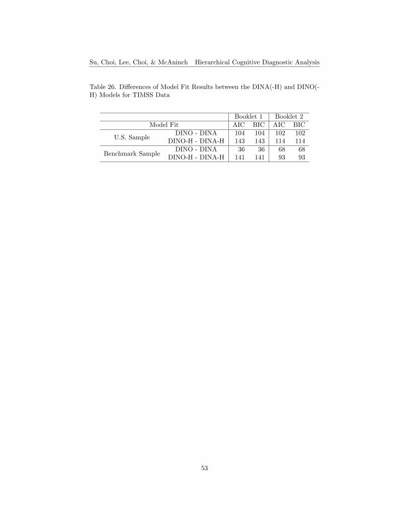
Su, Choi, Lee, Choi, & McAninch Hierarchical Cognitive Diagnostic Analysis
Table 26. Differences of Model Fit Results between the DINA(-H) and DINO(-H) Models for TIMSS Data
Booklet 1 Booklet 2Model Fit AIC BIC AIC BIC
U.S. SampleDINO - DINA 104 104 102 102
DINO-H - DINA-H 143 143 114 114
Benchmark SampleDINO - DINA 36 36 68 68
DINO-H - DINA-H 141 141 93 93
53
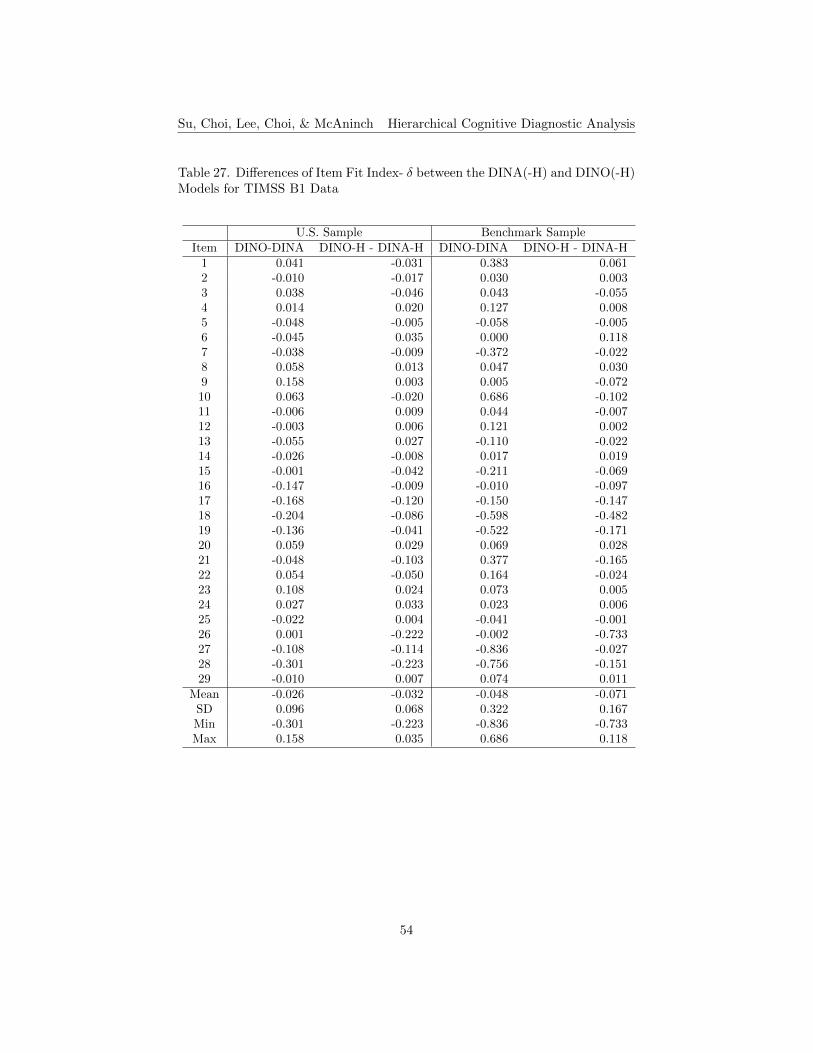
Su, Choi, Lee, Choi, & McAninch Hierarchical Cognitive Diagnostic Analysis
Table 27. Differences of Item Fit Index- δ between the DINA(-H) and DINO(-H)Models for TIMSS B1 Data
U.S. Sample Benchmark SampleItem DINO-DINA DINO-H - DINA-H DINO-DINA DINO-H - DINA-H
1 0.041 -0.031 0.383 0.0612 -0.010 -0.017 0.030 0.0033 0.038 -0.046 0.043 -0.0554 0.014 0.020 0.127 0.0085 -0.048 -0.005 -0.058 -0.0056 -0.045 0.035 0.000 0.1187 -0.038 -0.009 -0.372 -0.0228 0.058 0.013 0.047 0.0309 0.158 0.003 0.005 -0.07210 0.063 -0.020 0.686 -0.10211 -0.006 0.009 0.044 -0.00712 -0.003 0.006 0.121 0.00213 -0.055 0.027 -0.110 -0.02214 -0.026 -0.008 0.017 0.01915 -0.001 -0.042 -0.211 -0.06916 -0.147 -0.009 -0.010 -0.09717 -0.168 -0.120 -0.150 -0.14718 -0.204 -0.086 -0.598 -0.48219 -0.136 -0.041 -0.522 -0.17120 0.059 0.029 0.069 0.02821 -0.048 -0.103 0.377 -0.16522 0.054 -0.050 0.164 -0.02423 0.108 0.024 0.073 0.00524 0.027 0.033 0.023 0.00625 -0.022 0.004 -0.041 -0.00126 0.001 -0.222 -0.002 -0.73327 -0.108 -0.114 -0.836 -0.02728 -0.301 -0.223 -0.756 -0.15129 -0.010 0.007 0.074 0.011
Mean -0.026 -0.032 -0.048 -0.071SD 0.096 0.068 0.322 0.167Min -0.301 -0.223 -0.836 -0.733Max 0.158 0.035 0.686 0.118
54
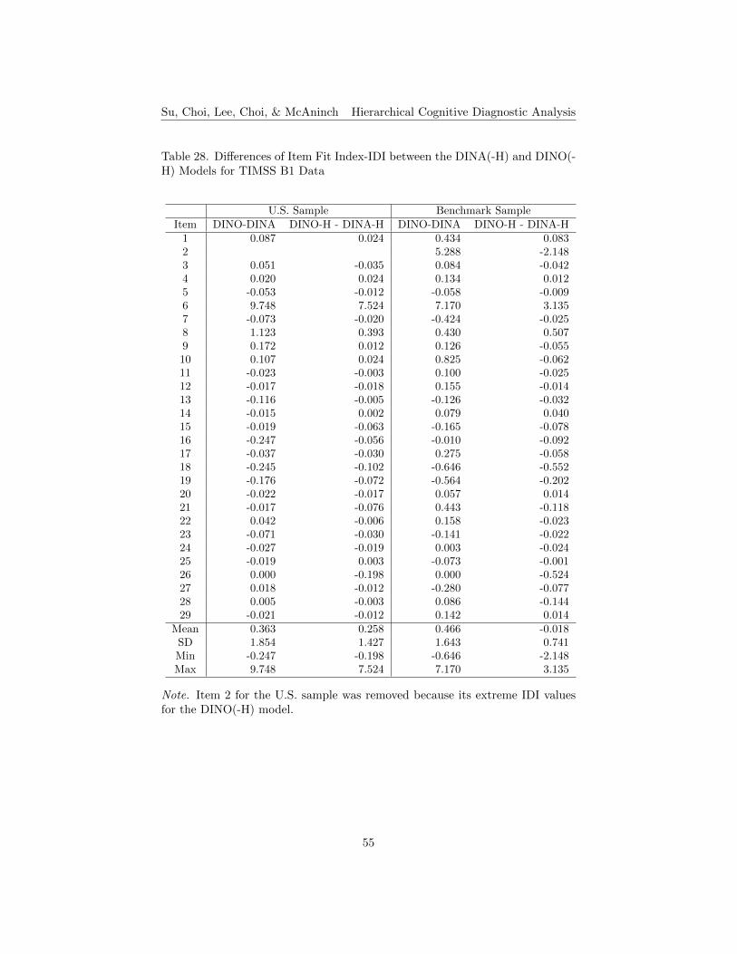
Su, Choi, Lee, Choi, & McAninch Hierarchical Cognitive Diagnostic Analysis
Table 28. Differences of Item Fit Index-IDI between the DINA(-H) and DINO(-H) Models for TIMSS B1 Data
U.S. Sample Benchmark SampleItem DINO-DINA DINO-H - DINA-H DINO-DINA DINO-H - DINA-H
1 0.087 0.024 0.434 0.0832 5.288 -2.1483 0.051 -0.035 0.084 -0.0424 0.020 0.024 0.134 0.0125 -0.053 -0.012 -0.058 -0.0096 9.748 7.524 7.170 3.1357 -0.073 -0.020 -0.424 -0.0258 1.123 0.393 0.430 0.5079 0.172 0.012 0.126 -0.05510 0.107 0.024 0.825 -0.06211 -0.023 -0.003 0.100 -0.02512 -0.017 -0.018 0.155 -0.01413 -0.116 -0.005 -0.126 -0.03214 -0.015 0.002 0.079 0.04015 -0.019 -0.063 -0.165 -0.07816 -0.247 -0.056 -0.010 -0.09217 -0.037 -0.030 0.275 -0.05818 -0.245 -0.102 -0.646 -0.55219 -0.176 -0.072 -0.564 -0.20220 -0.022 -0.017 0.057 0.01421 -0.017 -0.076 0.443 -0.11822 0.042 -0.006 0.158 -0.02323 -0.071 -0.030 -0.141 -0.02224 -0.027 -0.019 0.003 -0.02425 -0.019 0.003 -0.073 -0.00126 0.000 -0.198 0.000 -0.52427 0.018 -0.012 -0.280 -0.07728 0.005 -0.003 0.086 -0.14429 -0.021 -0.012 0.142 0.014
Mean 0.363 0.258 0.466 -0.018SD 1.854 1.427 1.643 0.741Min -0.247 -0.198 -0.646 -2.148Max 9.748 7.524 7.170 3.135
Note. Item 2 for the U.S. sample was removed because its extreme IDI valuesfor the DINO(-H) model.
55
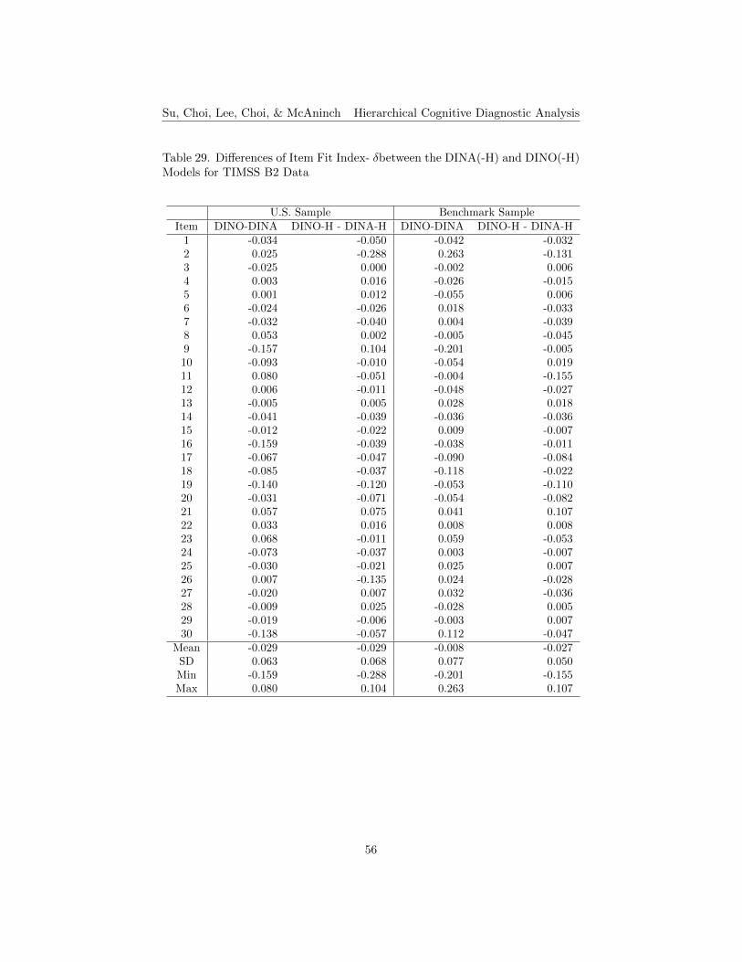
Su, Choi, Lee, Choi, & McAninch Hierarchical Cognitive Diagnostic Analysis
Table 29. Differences of Item Fit Index- δbetween the DINA(-H) and DINO(-H)Models for TIMSS B2 Data
U.S. Sample Benchmark SampleItem DINO-DINA DINO-H - DINA-H DINO-DINA DINO-H - DINA-H
1 -0.034 -0.050 -0.042 -0.0322 0.025 -0.288 0.263 -0.1313 -0.025 0.000 -0.002 0.0064 0.003 0.016 -0.026 -0.0155 0.001 0.012 -0.055 0.0066 -0.024 -0.026 0.018 -0.0337 -0.032 -0.040 0.004 -0.0398 0.053 0.002 -0.005 -0.0459 -0.157 0.104 -0.201 -0.00510 -0.093 -0.010 -0.054 0.01911 0.080 -0.051 -0.004 -0.15512 0.006 -0.011 -0.048 -0.02713 -0.005 0.005 0.028 0.01814 -0.041 -0.039 -0.036 -0.03615 -0.012 -0.022 0.009 -0.00716 -0.159 -0.039 -0.038 -0.01117 -0.067 -0.047 -0.090 -0.08418 -0.085 -0.037 -0.118 -0.02219 -0.140 -0.120 -0.053 -0.11020 -0.031 -0.071 -0.054 -0.08221 0.057 0.075 0.041 0.10722 0.033 0.016 0.008 0.00823 0.068 -0.011 0.059 -0.05324 -0.073 -0.037 0.003 -0.00725 -0.030 -0.021 0.025 0.00726 0.007 -0.135 0.024 -0.02827 -0.020 0.007 0.032 -0.03628 -0.009 0.025 -0.028 0.00529 -0.019 -0.006 -0.003 0.00730 -0.138 -0.057 0.112 -0.047
Mean -0.029 -0.029 -0.008 -0.027SD 0.063 0.068 0.077 0.050Min -0.159 -0.288 -0.201 -0.155Max 0.080 0.104 0.263 0.107
56
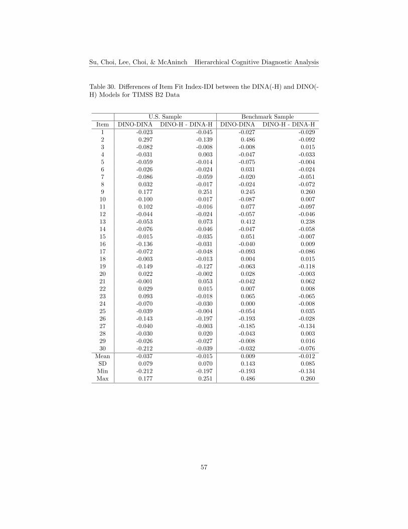
Su, Choi, Lee, Choi, & McAninch Hierarchical Cognitive Diagnostic Analysis
Table 30. Differences of Item Fit Index-IDI between the DINA(-H) and DINO(-H) Models for TIMSS B2 Data
U.S. Sample Benchmark SampleItem DINO-DINA DINO-H - DINA-H DINO-DINA DINO-H - DINA-H
1 -0.023 -0.045 -0.027 -0.0292 0.297 -0.139 0.486 -0.0923 -0.082 -0.008 -0.008 0.0154 -0.031 0.003 -0.047 -0.0335 -0.059 -0.014 -0.075 -0.0046 -0.026 -0.024 0.031 -0.0247 -0.086 -0.059 -0.020 -0.0518 0.032 -0.017 -0.024 -0.0729 0.177 0.251 0.245 0.26010 -0.100 -0.017 -0.087 0.00711 0.102 -0.016 0.077 -0.09712 -0.044 -0.024 -0.057 -0.04613 -0.053 0.073 0.412 0.23814 -0.076 -0.046 -0.047 -0.05815 -0.015 -0.035 0.051 -0.00716 -0.136 -0.031 -0.040 0.00917 -0.072 -0.048 -0.093 -0.08618 -0.003 -0.013 0.004 0.01519 -0.149 -0.127 -0.063 -0.11820 0.022 -0.002 0.028 -0.00321 -0.001 0.053 -0.042 0.06222 0.029 0.015 0.007 0.00823 0.093 -0.018 0.065 -0.06524 -0.070 -0.030 0.000 -0.00825 -0.039 -0.004 -0.054 0.03526 -0.143 -0.197 -0.193 -0.02827 -0.040 -0.003 -0.185 -0.13428 -0.030 0.020 -0.043 0.00329 -0.026 -0.027 -0.008 0.01630 -0.212 -0.039 -0.032 -0.076
Mean -0.037 -0.015 0.009 -0.012SD 0.079 0.070 0.143 0.085Min -0.212 -0.197 -0.193 -0.134Max 0.177 0.251 0.486 0.260
57
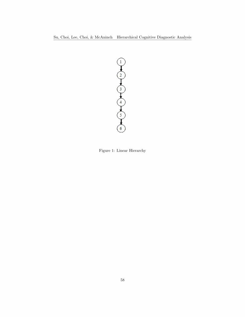
Su, Choi, Lee, Choi, & McAninch Hierarchical Cognitive Diagnostic Analysis
Figure 1: Linear Hierarchy
58
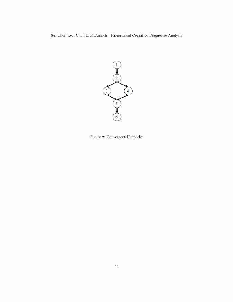
Su, Choi, Lee, Choi, & McAninch Hierarchical Cognitive Diagnostic Analysis
Figure 2: Convergent Hierarchy
59
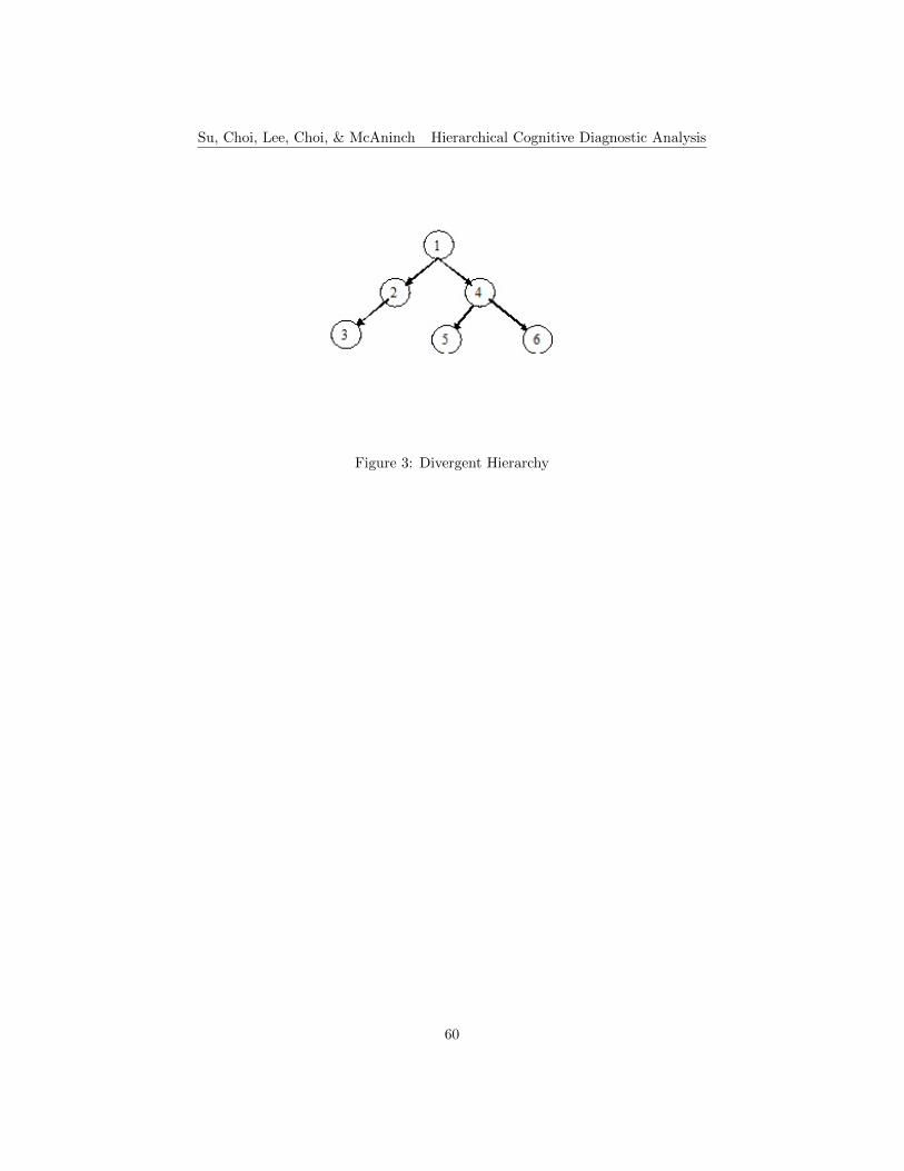
Su, Choi, Lee, Choi, & McAninch Hierarchical Cognitive Diagnostic Analysis
Figure 3: Divergent Hierarchy
60
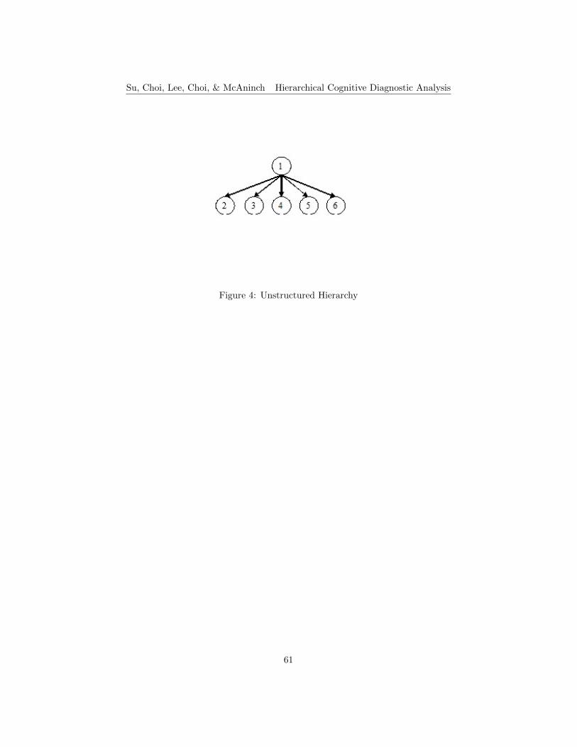
Su, Choi, Lee, Choi, & McAninch Hierarchical Cognitive Diagnostic Analysis
Figure 4: Unstructured Hierarchy
61
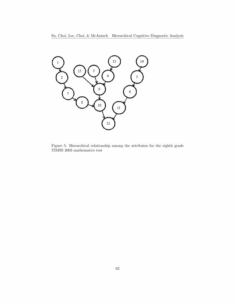
Su, Choi, Lee, Choi, & McAninch Hierarchical Cognitive Diagnostic Analysis
Figure 5: Hierarchical relationship among the attributes for the eighth gradeTIMSS 2003 mathematics test
62
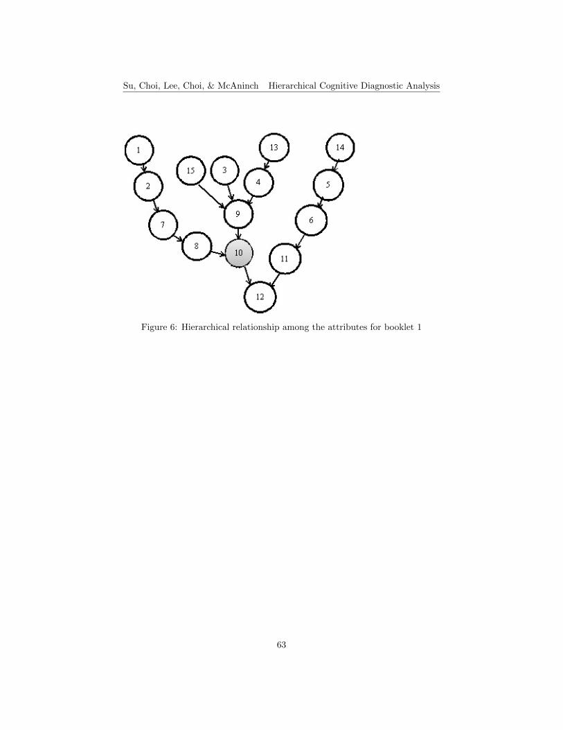
Su, Choi, Lee, Choi, & McAninch Hierarchical Cognitive Diagnostic Analysis
Figure 6: Hierarchical relationship among the attributes for booklet 1
63

Su, Choi, Lee, Choi, & McAninch Hierarchical Cognitive Diagnostic Analysis
Figure 7: Hierarchical relationships among the attributes for booklet 2
64