1 / 11

CEM: A Matching Method for Observational Datain the Social Sciences

S.M. Iacus (Univ. of Milan) & G. King (Harvard Univ.) & G. Porro (Univ. of Trieste)

Rennes, useR! 2009, July 8th - 10th

The problem of matching

Estimation of TE

Matching solutions in R(incomplete list)

CEM Overview

Infos

2 / 11

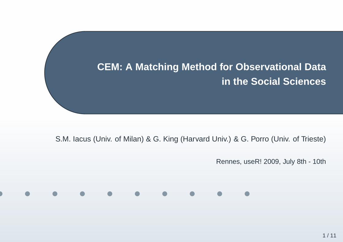
We consider an observational study with n observations. For each unit i

Yi = outcome Ti = treatment indicator X i = covariates

ESTIMATION GOAL: the treatment effect

TEi = Yi(Ti = 1) − Yi(Ti = 0) = Yi(1) − Yi(0)

but Yi(0) is not observed. For the treated unit i with covariates Xi, it is natural

to look for another unit j in the sample for which Yj(0) is observed and such

that Xj ≃ X i

MATCHING GOAL: for each treated unit i find the “twin” control unit j (i.e. with

Xj ≃ Xi) in order to reduce bias in the estimation of TEi

Matching solutions in R (incomplete list)

Estimation of TE

Matching solutions in R(incomplete list)

CEM Overview

Infos

3 / 11

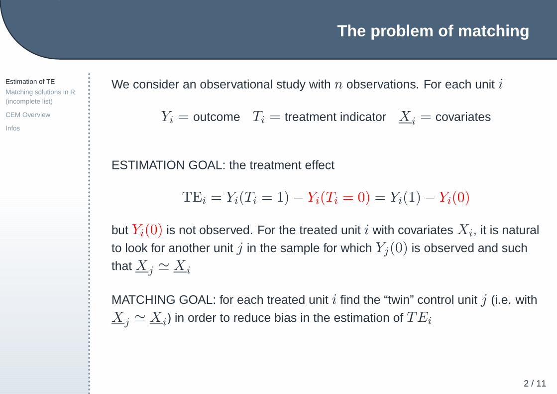
� MatchIt : (pscore, mahalanobis, etc)

� Matching : (genetic matching, pscore, etc)

� optmatch : (full optimal matching)

� rrp : (random recursive partitioning)

� arm : (single nearest neighbour)

� SpectralGEM : (spectral graph theory)

� analogue : (analogue matching, nearest neighbour)

� PSAgraphics (diagnotic)

� RItools (diagnostic)

CEM Overview

Estimation of TE

Matching solutions in R(incomplete list)

CEM Overview

Infos

4 / 11

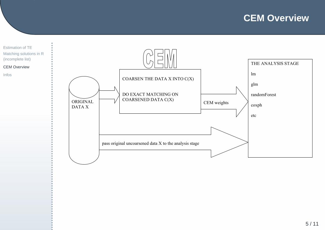
Coarsened Exact Matching (CEM), is a simple (and ancient) method of causal

inference, with unexplored powerful properties. CEM is as simple as

CEM Overview

Estimation of TE

Matching solutions in R(incomplete list)

CEM Overview

Infos

4 / 11

Coarsened Exact Matching (CEM), is a simple (and ancient) method of causal

inference, with unexplored powerful properties. CEM is as simple as

1. Temporarily coarsen X as much as you’re willing (e.g., for education:

grade school, high school, college, graduate);

CEM Overview

Estimation of TE

Matching solutions in R(incomplete list)

CEM Overview

Infos

4 / 11

Coarsened Exact Matching (CEM), is a simple (and ancient) method of causal

inference, with unexplored powerful properties. CEM is as simple as

1. Temporarily coarsen X as much as you’re willing (e.g., for education:

grade school, high school, college, graduate);

2. Perform exact matching on the coarsened data C(X), sort observations

into strata and prune any stratum with 0 treated or 0 control units, i.e. set

weight=0 for pruned observations and CEM weights to matched units;

CEM Overview

Estimation of TE

Matching solutions in R(incomplete list)

CEM Overview

Infos

4 / 11

Coarsened Exact Matching (CEM), is a simple (and ancient) method of causal

inference, with unexplored powerful properties. CEM is as simple as

1. Temporarily coarsen X as much as you’re willing (e.g., for education:

grade school, high school, college, graduate);

2. Perform exact matching on the coarsened data C(X), sort observations

into strata and prune any stratum with 0 treated or 0 control units, i.e. set

weight=0 for pruned observations and CEM weights to matched units;

3. use the original uncoarsened data X (with appropriate weights) in your

analysis, except those units pruned.

Maximum imbalance is controlled ex-ante by the choice of coarsening

CEM Overview

Estimation of TE

Matching solutions in R(incomplete list)

CEM Overview

Infos

5 / 11

COARSEN THE DATA X INTO C(X)

DO EXACT MATCHING ON

COARSENED DATA C(X)

CEM weights

pass original uncoarsened data X to the analysis stage

ORIGINAL

DATA X

THE ANALYSIS STAGE

lm

glm

randomForest

coxph

etc

CEM package

6 / 11

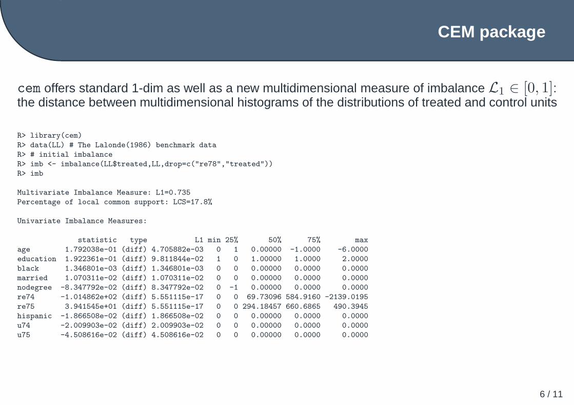
cem offers standard 1-dim as well as a new multidimensional measure of imbalance L1 ∈ [0, 1]:the distance between multidimensional histograms of the distributions of treated and control units

R> library(cem)

R> data(LL) # The Lalonde(1986) benchmark data

R> # initial imbalance

R> imb <- imbalance(LL$treated,LL,drop=c("re78","treated"))

R> imb

Multivariate Imbalance Measure: L1=0.735

Percentage of local common support: LCS=17.8%

Univariate Imbalance Measures:

statistic type L1 min 25% 50% 75% max

age 1.792038e-01 (diff) 4.705882e-03 0 1 0.00000 -1.0000 -6.0000

education 1.922361e-01 (diff) 9.811844e-02 1 0 1.00000 1.0000 2.0000

black 1.346801e-03 (diff) 1.346801e-03 0 0 0.00000 0.0000 0.0000

married 1.070311e-02 (diff) 1.070311e-02 0 0 0.00000 0.0000 0.0000

nodegree -8.347792e-02 (diff) 8.347792e-02 0 -1 0.00000 0.0000 0.0000

re74 -1.014862e+02 (diff) 5.551115e-17 0 0 69.73096 584.9160 -2139.0195

re75 3.941545e+01 (diff) 5.551115e-17 0 0 294.18457 660.6865 490.3945

hispanic -1.866508e-02 (diff) 1.866508e-02 0 0 0.00000 0.0000 0.0000

u74 -2.009903e-02 (diff) 2.009903e-02 0 0 0.00000 0.0000 0.0000

u75 -4.508616e-02 (diff) 4.508616e-02 0 0 0.00000 0.0000 0.0000

CEM package

7 / 11

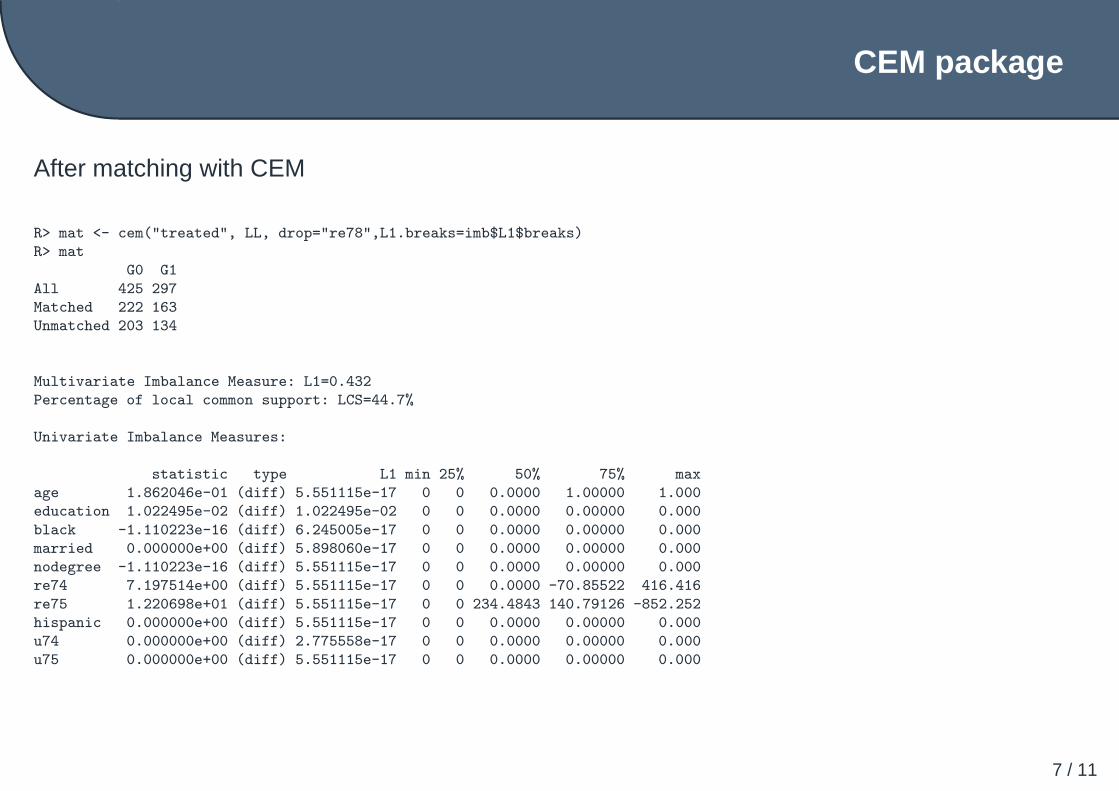
After matching with CEM

R> mat <- cem("treated", LL, drop="re78",L1.breaks=imb$L1$breaks)

R> mat

G0 G1

All 425 297

Matched 222 163

Unmatched 203 134

Multivariate Imbalance Measure: L1=0.432

Percentage of local common support: LCS=44.7%

Univariate Imbalance Measures:

statistic type L1 min 25% 50% 75% max

age 1.862046e-01 (diff) 5.551115e-17 0 0 0.0000 1.00000 1.000

education 1.022495e-02 (diff) 1.022495e-02 0 0 0.0000 0.00000 0.000

black -1.110223e-16 (diff) 6.245005e-17 0 0 0.0000 0.00000 0.000

married 0.000000e+00 (diff) 5.898060e-17 0 0 0.0000 0.00000 0.000

nodegree -1.110223e-16 (diff) 5.551115e-17 0 0 0.0000 0.00000 0.000

re74 7.197514e+00 (diff) 5.551115e-17 0 0 0.0000 -70.85522 416.416

re75 1.220698e+01 (diff) 5.551115e-17 0 0 234.4843 140.79126 -852.252

hispanic 0.000000e+00 (diff) 5.551115e-17 0 0 0.0000 0.00000 0.000

u74 0.000000e+00 (diff) 2.775558e-17 0 0 0.0000 0.00000 0.000

u75 0.000000e+00 (diff) 5.551115e-17 0 0 0.0000 0.00000 0.000

Diagnostic tool

8 / 11

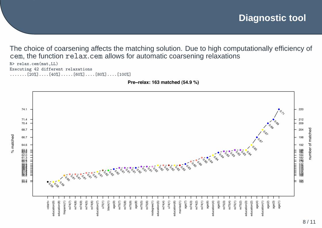
The choice of coarsening affects the matching solution. Due to high computationally efficiency ofcem, the function relax.cem allows for automatic coarsening relaxationsR> relax.cem(mat,LL)

Executing 42 different relaxations

.......[20%]....[40%].....[60%]....[80%]....[100%]

Pre−relax: 163 matched (54.9 %)

● ●●

●● ● ●

● ●●

● ●●

● ● ● ●● ● ●

● ● ● ● ●●

●●

● ●

●

●● ●

● ● ●

●

●

●

●

●

●

<sta

rt>

education(9

)

education(8

)

his

panic

(1)

re74(7

)

re74(8

)

re74(9

)

re74(5

)

re74(6

)

education(7

)

u75(1

)

bla

ck(1

)

age(9

)

re75(7

)

re75(8

)

re75(9

)

age(8

)

re75(5

)

re75(6

)

nodegre

e(1

)

education(5

)

re74(4

)

u74(1

)

education(6

)

marr

ied(1

)

age(7

)

re74(3

)

re74(2

)

re74(1

)

age(6

)

education(4

)

age(5

)

re75(3

)

re75(4

)

re75(1

)

re75(2

)

education(3

)

education(2

)

age(4

)

education(1

)

age(2

)

age(3

)

age(1

)

54.955.2

56.656.957.257.657.958.258.658.959.359.660.360.661.362.062.663.063.3

64.6

66.7

68.7

70.4

71.4

74.1

163164

168169170171172173174175176177179180182184186187188

192

198

204

209

212

220

0.590.59

0.590.60

0.610.610.61

0.610.61

0.610.620.62

0.620.610.610.610.62

0.610.610.62

0.620.620.620.620.63

0.630.60

0.600.600.64

0.640.64

0.630.63

0.630.630.64

0.650.67

0.670.69

0.690.71

num

ber

of

matc

hed

% m

atc

hed

ATT estimation and extrapolation

9 / 11

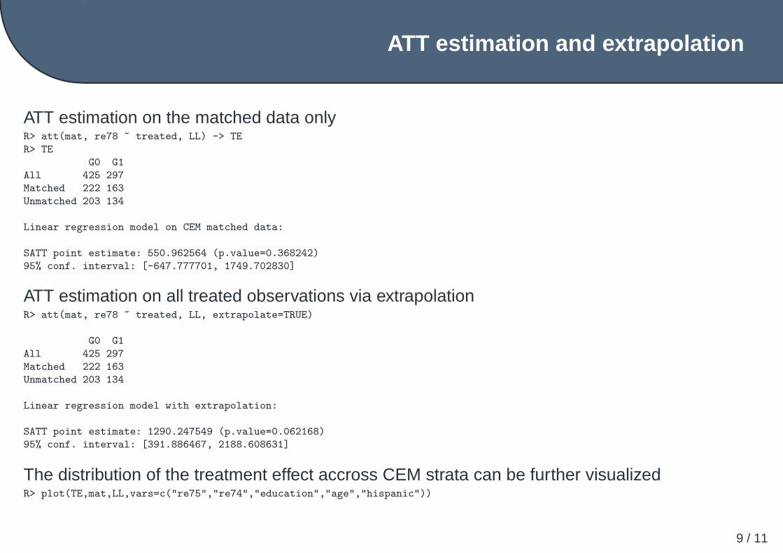
ATT estimation on the matched data onlyR> att(mat, re78 ~ treated, LL) -> TE

R> TE

G0 G1

All 425 297

Matched 222 163

Unmatched 203 134

Linear regression model on CEM matched data:

SATT point estimate: 550.962564 (p.value=0.368242)

95% conf. interval: [-647.777701, 1749.702830]

ATT estimation on all treated observations via extrapolationR> att(mat, re78 ~ treated, LL, extrapolate=TRUE)

G0 G1

All 425 297

Matched 222 163

Unmatched 203 134

Linear regression model with extrapolation:

SATT point estimate: 1290.247549 (p.value=0.062168)

95% conf. interval: [391.886467, 2188.608631]

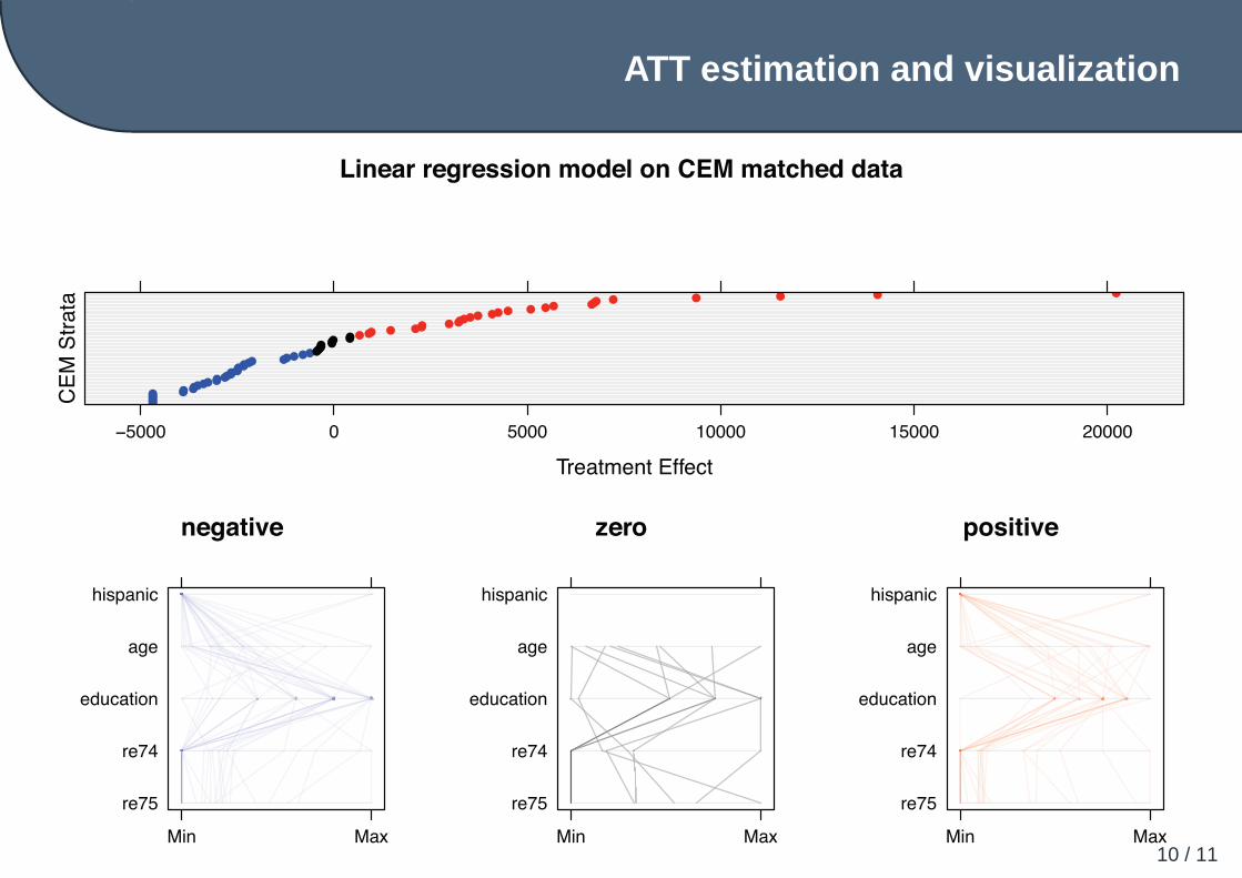
The distribution of the treatment effect accross CEM strata can be further visualizedR> plot(TE,mat,LL,vars=c("re75","re74","education","age","hispanic"))

ATT estimation and visualization

10 / 11

Linear regression model on CEM matched data

Treatment Effect

CE

M S

trata

−5000 0 5000 10000 15000 20000

●●●●●●● ●●●●●

●●●●●●

●●●●●●●●●

●●●●●●

●●●●●●●

●●●●● ● ●●●●●●●

●● ●●● ● ●● ●●●● ● ● ● ●

negative

re75

re74

education

age

hispanic

Min Max

zero

re75

re74

education

age

hispanic

Min Max

positive

re75

re74

education

age

hispanic

Min Max

For more information

Estimation of TE

Matching solutions in R(incomplete list)

CEM Overview

Infos

11 / 11

For the latest version of the manuscript, R and Stata software, visit

http://GKing.Harvard.edu/cem