Embed Size (px)
Citation preview

Cellular Service Demand:Biased Beliefs, Learning, and Bill Shock
Michael D. Grubb and Matthew Osborne
Online Appendix
May 2014
A Data Details
A.1 University Price Data
Table 6: Popular Plan Price Menu
Plan 0 ($14.99) Plan 1 ($34.99) Plan 2 ($44.99) Plan 3 ($54.99)Date Q p OP Net Q p OP Net Q p OP Net Q p OP Net
8/02 - 10/02 - - - - 280 40 free not 653 40 free not 875 35 free not10/02 - 12/02 0 11 free free 280 40 free not 653 40 free not 875 35 free not12/02 - 1/03 0 11 free free 350 40 free not 653 40 free not 875 35 free not1/03 - 2/03 0 11 free free 280 40 free not 653 40 free not 875 35 free not2/03 - 3/03 0 11 free free 380 40 free not 653 40 free not 875 35 free not3/03 - 9/03 0 11 free free 288 45 free not 660 40 free not 890 40 free not9/03 - 1/04 0 11 not free 388 45 free not 660 40 free not 890 40 free not1/04 - 4/04 0 11 not free 388 45 free not 660 40 free free 890 40 free not4/04 - 5/04 0 11 not free 388 45 free not 1060 40 free free 890 40 free not5/04 - 7/04 0 11 not free 288 45 free not 760 40 free free 890 40 free not
Entries describe the calling allowance (Q), the overage rate (p), whether off-peak calling is free or not (OP), andwhether in-network calling is free or not (Net). Bold entries reflect price changes that apply to new plan subscribers.The Bold italics entry reflects the one price change which also applied to existing plan subscribers. Some termsremained constant: Plan 0 always offered Q = 0, p = 11, and free in-network. Plans 1-3 always offered free off-peak.
Prices of the four popular plans are described for all dates in Table 6. This price series was
inferred from billing data rather than directly observed. For each plan and each date, we infer the
total number of included free minutes by observing the number of minutes used prior to an overage
in the call-level data. (This calculation is complicated by the fact that some plans offered free in-
network calls, and our call-level data does not identify whether an incoming call was in-network.)
We were able to reliably infer this pricing information for popular plans from August 2002 to July
2004. We exclude other dates and the 11 percent of bills from unpopular plans (national plans,
free-long-distance plans, and expensive local plans), grouping them with the outside option in our
1

structural model. In fact, we treat switching to an unpopular plan the same as quitting service,
hence we also drop all remaining bills once a customer switches to an unpopular plan, even if they
eventually switch back to a popular plan.
As stated in Section II.A, an additional 7 percent of individuals are excluded from our structural
estimation due to data problems. In particular, we exclude individuals with substantially negative
bills, indicating either billing errors or ex post renegotiated refunds that are outside our model.
Also excluded are individuals who have infeasible choices recorded (plans outside the choice set or
negative in-network calling) and 8 individuals for whom we could not find starting points (initial
parameter values from which to begin maximizing the likelihood) with positive likelihood.
A.2 Public Price Data
Table 7 shows a subset of data obtained from EconOne: publicly available local calling plans for
October 2003 in the same geographic market as the university. (Sprint did not offer local plans.)
Table 7: Publicly Available Local Calling Plans - October 2003
AT&T Cingular VerizonPlan M Q p M Q p M Q p
1 29.99 350 0.45 29.99 300 0.49 29.99 300 0.452 39.99 600 0.40 39.99 600 0.49 39.99 500 0.453 49.99 800 0.40 49.99 1000 0.45 49.99 700 0.404 59.99 1050 0.35 69.99 1200 0.45 59.99 1000 0.40
A.3 Additional Evidence of Inattention
If consumers are attentive to the remaining balance of included minutes during the billing cycle they
should use this information to continually update their beliefs about the likelihood of an overage
and a high marginal price ex post. Following an optimal dynamic program, an attentive consumer
should (all else equal) reduce her usage later in the month following unexpectedly high usage
earlier in the month. This prediction should be true for any consumers who are initially uncertain
whether they will have an overage in the current month. For these consumers, the high usage
shock early in the month increases the likelihood of an overage, thereby increasing their expected
ex post marginal price, and causing them to be more selective about calls. If calling opportunities
arrived independently throughout the month, this strategic behavior by the consumer would lead
to negative correlation between early and late usage within a billing period. However, looking for
2

negative correlation in usage within the billing period is a poor test for this dynamic behavior
because it is likely to be overwhelmed by positive serial correlation in taste shocks.
To test for dynamic behavior by consumers within the billing period, we use our data set of
individual calls to construct both fortnightly and weekly measures of peak usage. A simple regres-
sion of usage on individual fixed effects and lagged usage shows strong positive serial correlation.
However, we take advantage of the following difference: Positive serial correlation between taste
shocks in periods t and (t−1) should be independent of whether periods t and (t−1) are in the same
or adjacent billing cycles. However, following unexpectedly high usage in period (t− 1), consumers
should cut back usage more in period t if the two periods are in the same billing cycle. Thus by
including an interaction effect between lagged usage and an indicator for the lag being in the same
billing cycle as the current period, we can separate strategic behavior within the month from serial
correlation in taste shocks.
Table 8 shows a regression of log usage on lagged usage and the interaction between lagged usage
and an indicator equal to 1 if period (t− 1) is in the same billing cycle as period t. We also include
time and individual fixed effects and correct for bias induced by including both individual fixed
effects and lags of the dependent variable in a wide but short panel (Roodman, 2009). Reported
analysis is for plan 1, the most popular three-part tariff. As expected, positive serial correlation
in demand shocks leads to a positive and significant coefficient on lagged usage in the full sample
(column 1) and most subsamples (columns 2-6). If consumers adjust their behavior dynamically
within the billing cycle in response to usage shocks, then we expect the interaction effect to be
negative. In the full sample (column 1) the interaction effect has a positive point estimate, but is
not significantly different from zero. This result suggests that consumers are not attentive to past
usage during the course of the month.
Table 8: Dynamic Usage Pattern at Fortnightly Level.
(1) (2) (3) (4) (5) (6)Overage Percentage 0-100% 0 1-29% 30-70% 71-99% 100%
ln(qt−1) 0.649*** 0.609*** 0.522*** 0.514*** -1.046 0.958***(0.0270) (0.0524) (0.0437) (0.0695) (1.060) (0.0441)
SameBill*ln(qt−1) 0.00692 0.0150 0.0256 -0.0222 -0.0837 3.685(0.0108) (0.0197) (0.0182) (0.0229) (1.174) (4.745)
Observations 9062 3717 3222 1830 217 76Number of individuals 385 166 130 87 11 6
Dependent variable ln(qt). Standard errors in parentheses. Time and individual fixed effects.
Key: *** p<0.01, ** p<0.05, * p<0.1
3

Consumers who either never have an overage (43 percent of plan 1 subscribers) or always have
an overage (3 percent of plan 1 subscribers) should be relatively certain what their ex post marginal
price will be, and need not adjust calling behavior during the month. For instance, consumers who
always make overages may only make calls worth more than the overage rate throughout the month.
For such consumers we would expect to find no interaction effect, and this may drive the result when
all consumers are pooled together as in our first specification. As a result, we divide consumers
into groups by the fraction of times within their tenure that they have overages. We repeat our
first specification for different overage-risk groups in Columns 2-6 of Table 8. The interaction effect
is indistinguishable from zero in all overage risk groups. Moreover, in unreported analysis, more
flexible specifications that include nonlinear terms1 and a similar analysis at the weekly rather than
fortnightly level all estimate an interaction effect indistinguishable from zero. There is simply no
evidence that we can find that consumers strategically cut back usage at the end of the month
following unexpectedly high initial usage. We conclude that consumers are inattentive to their
remaining balance of included minutes during the billing cycle.
A.4 Plan Switching Calculations
We make two calculations for each switch from an existing plan j to an alternate plan j′ that cannot
be explained by a price cut for plan j′. First, we calculate how much the customer would have saved
had they signed up for the new plan j′ initially, holding their usage from the original plan j fixed.
By this calculation, average savings are $10.87 to $15.24 per month and 60 to 61 percent of switches
save consumers money. We calculate bounds because we cannot always distinguish in-network and
out-of-network calls. Average savings are statistically greater than zero at the 99 percent level. The
60-61 percent rates of switching in the “right” direction are statistically greater than 50 percent at
the 95 percent level. This calculation is based on 99 of the 136 switches which cannot be explained
by price decreases. The remaining 37 switches occur so soon after the customer joins that there is
no usage data prior to the switch that is not from a pro-rated bill.
Second, we calculate how much money the customer would have lost had they remained on
existing plan j rather than switching to the new plan j′, now holding usage from plan j′ fixed. By
this calculation, average savings are $13.80 to $24.56 per month, and 61 to 69 percent of switches
save money. This calculation is based on 132 of the 137 switches which can not be explained by
1Average qt will vary with expected marginal price, which is proportional to the probability of an overage. Theprobability of an overage in a billing period which includes periods t and (t− 1) increases nonlinearly in qt−1. In onespecification, we first fit a probit on the likelihood of an overage as a function of the first fortnights usage, and thenused the estimated coefficients to generate overage probability estimates for all fortnights. We then included these(lagged) values as explanatory variables. In an alternative specification we added polynomial terms of lagged qt−1.
4

price decreases. The calculation cannot be made for the remaining 5 switches since there is no
usage data following the switch that is not from a pro-rated bill. Figures are significant at the 95
percent or 99 percent confidence level.
As explained in Section II.B, the first and second calculations described above provide lower
and upper bounds, respectively, on the benefits of switching plans. We therefore conclude that
consumers’ expected benefit from switching is between $10.87 and $24.56 per month and 60 to 69
percent of switches save money.
B Model Details
A Model Guide: Tables 9 - 12 provide a guide to model parameters.
B.1 Derivation of optimal calling threshold
Define q(p, θkit) ≡ arg maxq(V(q, θkit
)− pq
)to be a consumer’s demand for category-k calls given a
constant marginal price p. (This is the quantity of category-k calls valued above p.) A consumer’s
inverse demand for category-k calls is Vq(qkit, θ
kit) =
(1− qkitθ
kit
)/β and thus:
q(p, θkit) = θkit (1− βp) = θkitq(p). (12)
Conditional on tariff choice j with free off-peak calling, consumer i chooses her period t peak
threshold vpkitj to maximize her expected utility conditional on her period t information =it:
vpkitj = arg maxv∗
E[V(q(v∗, θpkit ), θpkit
)− Pj
(q(v∗, θpkit )
)| =it
].
Let Fit be the cumulative distribution of θpkit as perceived by consumer i at time t. The first-order
condition for the consumer’s problem is
∫ θ
θVq
(q(v∗, θpkit ), θpkit
) d
dv∗q(v∗, θpkit )dFit(θ
pkit ) =
∫ θ
θ∗j (v∗)pj
d
dv∗q(v∗, θpkit )dFit(θ
pkit ), (13)
where θ∗j (v∗) is the peak type which consumes exactly Qj units: q(v∗, θ∗j (v∗)) = Qj . Equation
(13) is similar to Borenstein’s (2009) first-order condition. Unlike Borenstein (2009), we assume
Vq(q(v∗, θkit), θ
kit) is equal to v∗ by definition. (Notice that substituting q
(v∗, θkit
)= θkit (1− βv∗)
5

Table 9: Model Guide: Payments, Preferences, and Usage
Parameter Description Distribution or equation
qbillableitj billable minutes qbillableitj = qpkit +OPjqopit
OPj indicator for costly off-peak plan j constant
Pj price plan j Pj (qit) = Mj + pj max{0, qbillableitj −Qj}Mj monthly fee plan j constant
Qj allowance plan j constant
pj overage rate plan j constant
V value function V(qkit, θ
kit
)= 1
β qkit
(1− 1
2
(qkit/θ
kit
))uitj utility function uitj =
∑k∈{pk,op} V
(qkit, θ
kit
)− Pj (qit) + ηitf
Uitj expected utility equation (5)
β price sensitivity constant
O outside good utility constant
PC plan consideration Pr. constant
ηitf logit error iid logit
θkit # calling opportunities θkit = max{0, θkit}θkit latent taste shock θit = µi + εit
vkitj calling threshold equation (4)
v∗itj calling threshold vector v∗itj = (vpkitj , vopitj)
q(vkitj) Frac. calling opp. value > vkitj q(vkitj) = (1− βvkitj)qkit minutes of calling (usage) qkit = θkitq(v
kitj)
Subscripts and superscripts denote customer i, time t, plan j, firm f , and calling category k ∈ {pk, op}.
6

Table 10: Model Guide: Tastes & Signals
Parameter Description Distribution
µpki1
µpki
µopi
Point Estimate µpki
Peak Type
Off-Peak Type
N
µpk0
µpk0
µop0
,
(σpkµ )2 ρµ,pkσpkµ σ
pkµ ρµ,opσ
opµ σ
pkµ
ρµ,pkσpkµ σ
pkµ (σpkµ )2 ρµσ
pkµ σ
opµ
ρµ,opσopµ σ
pkµ ρµσ
pkµ σ
opµ (σopµ )2
sit
εpkit
εopit
Signal
Peak Shock
Off-Peak Shock
N
0
0
0
,
1 ρs,pkσpkε ρs,opσ
opε
ρs,pkσpkε (σpkε )2 ρεσ
pkε σ
opε
ρs,opσopε ρεσ
pkε σ
opε (σopε )2
Table 11: Model Guide: Beliefs and Biases
Parameter Description Equation
δ overconfidence
µpkit updated point est. Bayes rule, equation (17)
σt SD[µpki | µpkit ] Bayes rule (t > 1) equation (18)
σt SD[µpki | µpkit ] σt = δσt
µpkθit E[θpkit | sit
]equation (6)
σθt SD[θpkit | sit
]equation (7)
σθt SD[θpkit | sit
]σθt = δσθt
b1 aggregate mean bias b1 = µpk0 − µpk0
b2 conditional mean bias b2 = 1− Cov(µpki ,µpki1 )
V ar(µpki1 )= 1− ρµ,pk
σpkµ
σpkµ. equation (8)
Operators E and SD denote population moments, while E and SD are with respect to individual i’s beliefs.
7

Table 12: Model Guide: Near-9pm Calling Parameters
Parameter Description Distribution or equation
rk,9it share of k-calling near 9pm rk,9it censored on [0, 1]
rk,9it latent shock rk,9it = αk,9i + ek,9it
αpk,9i pk-9pm type αpk,9i ∼ N(µpk,9α , (σpk,9α )2)
ek,9it pk-9pm shock ek,9it ∼ N(0, (σk,9e )2), iid across i, t, and k.
αop,9i op-9pm type Defined implicitly by equation (9)
Subscripts and superscripts denote customer i, time t, and calling category k ∈ {pk, op}.
from equation (12) into Vq(qkit, θ
kit) yields v∗). Thus equation (13) reduces to:
v∗ = pj
∫ θθ∗j (v∗)
ddv∗ q(v
∗, θpkit )dFit(θpkit )∫ θ
θddv∗ q(v
∗, θpkit )dFit(θpkit )
.
With multiplicative separability (equation (12)), θ∗j (v∗) = Qj/q (v∗) and d
dv∗ q(v∗, θpkit ) = θpkit
ddv∗ q (v∗),
so we can factor out and cancel ddv∗ q (v∗). This simplification yields equation (4). It is apparent by
inspection that equation (4) has a unique solution.
Equation (4) may seem counter-intuitive, because the optimal vpkitj is greater than the expected
marginal price, pj Pr(q(vpkitj , θpkit ) > Qj | =it). This is because the reduction in consumption from
raising vpkitj is proportional to θpkit . Raising vpkitj cuts back on calls valued at vpkitj more heavily in high
demand states when they cost pj and less heavily in low demand states when they cost 0.
Figure 9 plots the optimal calling threshold vpkitj as a function of consumer beliefs and the
corresponding plan choice. The distinct regions visible on the contour plot correspond to the plan
choice regions identified in Figure 7. Figure 9 shows that, on three-part tariffs, vpkitj increases with
the perceived mean and variance of calling opportunities because both increase the upper tail of
usage and hence the likelihood of paying overage fees. Figure 9 also shows that consumers who
choose a three-part tariff use calling thresholds that are small relative to the overage rates of $0.35 or
$0.45 per minute. This is because if the perceived likelihood of an overage were large the consumer
would have chosen a larger plan.
B.2 Optimal calling threshold under bill-shock regulation
For simplicity we temporarily drop the peak superscript as well as customer, date, and plan sub-
scripts. Given bill-shock regulation, a consumer will begin the billing cycle consuming all peak
8

0.000.020.040.060.080.100.120.14
µ~θi1
σ~ θ1
−200 0 250 500 750 1000
010
020
030
0
Figure 9: Calling threshold vpkitj as a function of initial beliefs {µθi1, σθ1} and the correspondingplan choice (shown in Figure 7) implied by the model evaluated at fall 2002 prices given β = 2.
calls above some threshold v∗ but raise this calling threshold to the overage rate p upon receiving
a bill-shock alert that the allowance Q has been reached.
Let θ∗ be the peak type which consumes exactly Q units given initial calling threshold v∗:
q(v∗, θ∗) = Q. If θ < θ∗ then the customer has a total of θ calling opportunities, makes θq (v∗) < Q
calls with value V (q (v∗, θ) , θ) and never receives a bill-shock alert. If θ > θ∗ then a bill-shock alert
is received and Figure 10 illustrates demand curves and calling thresholds before and after the alert.
Prior to receiving a bill-shock alert, the customer has θ∗ calling opportunities. Of these, fraction
q (v∗) are worth more than v∗ so that prior to the alert the consumer makes θ∗q (v∗) = Q calls with
total value V (Q, θ∗) and declines θ∗ (1− q (v∗)) calling opportunities. After receiving a bill-shock
warning, the customer has θa = θ − θ∗ additional calling opportunities. Of these, fraction q (p)
are worth more than the overage rate p so that after the alert the consumer makes an additional
θaq (p) calls with total value V (q (p, θa) , θa).
*
Q pre-alert calls worth more than v*
q
𝜃𝑎𝑞�(𝑝) post-alert calls worth more than p
$
v*
1 𝛽⁄ p
pre-alert calls declined post-alert calls declined
Figure 10: Inverse demand curves and calling thresholds before and after a bill-shock alert.
9

Notice that calls with the highest value 1/β are made both before and after the alert. This is
because the demand curves’ ordering of calls from high to low value is not chronological. Both low
and high value calls arrive throughout the month.
We now characterize the optimal calling threshold v∗ with bill-shock alerts. The consumer
chooses v∗ to maximize
U = −M +
∫ θ∗
0V (q (v∗, θ) , θ) f (θ) dθ +
∫ ∞θ∗
(V (Q, θ∗) + V (q (p, θa) , θa)− pq (p, θa)) f (θ) dθ,
where θ∗ = Q/q (v∗) and θa = θ − θ∗. After canceling terms (recognizing that q (v∗, θ∗) = Q,
q (p, 0) = 0, and V (0, θ) = 0) and substituting v∗ = Vq (q (v∗, θ) , θ) and dθa/dv∗ = −dθ∗/dv∗, the
first derivative is
dU
dv∗=
∫ θ∗
0v∗
d
dv∗q (v∗, θ) f (θ) dθ +
dθ∗
dv∗
∫ ∞θ∗
(Vθ (Q, θ∗)− Vθ (q (p, θa) , θa)) f (θ) dθ.
The multiplicative demand assumption implies ddv∗ q (v∗, θ) = θ d
dv∗ q (v∗) and dθ∗/dv∗ = −(Q/q2 (v∗)) ddv∗ q (v∗).
Therefore the ddv∗ q (v∗) terms cancel and the first-order condition is
v∗∫ θ∗
0θf (θ) dθ =
Q
q2 (v∗)
∫ ∞θ∗
(Vθ (Q, θ∗)− Vθ (q (p, θa) , θa)) f (θ) dθ.
Notice that because Vθ (q, θ) = q2/(2βθ2
)and q (p, θ) = θq (p) it holds that Vθ (q (p, θ) , θ) =
q2 (p) /2β is independent of θ. Substituting this expression in yields
v∗∫ θ∗
0θf (θ) dθ =
Q
2β
(1−
(q (p)
q (v∗)
)2)
(1− F (θ∗)) .
Rearranging terms, this expression is equivalent to
v∗ =Q
2β
(1−
(q (p)
q (v∗)
)2)
(1− F (θ∗))∫ θ∗0 θf (θ) dθ
, (14)
which characterizes v∗ given θ∗ = Q/q (v∗) and q (v∗) = 1− βv∗.
B.3 Bayesian Updating
In this appendix we use operators E and V to denote mean and variance in the population or given
objective probabilities. We use operators E and V to denote mean and variance given an individual
consumers’ subjective beliefs.
10

Updating from signal sit At the beginning of each period, each consumer receives a signal sit
that is informative about the taste innovation εit. Given the joint distribution of εit and sit and
the restriction ρs,op = ρs,pkρε, conditional on the signal sit: εit is normally distributed with mean
E([εpkit εopit
]| sit
)=[ρs,pkσ
pkε sit ρs,pkρεσ
opε sit
],
and variance
V([εpkit εopit
]| sit
)=
(σpkε )2(
1− ρ2s,pk
)ρεσ
pkε σ
opε
(1− ρ2
s,pk
)ρεσ
pkε σ
opε
(1− ρ2
s,pk
)(σopε )
2(1− ρ2
s,pkρ2ε)
.
However, as consumers underestimate the unconditional standard deviations of sit and εpkit by a
factor δ, consumers perceive the conditional distribution to be normal with mean
E([εpkit εopit
]| sit
)=
[ρs,pkσ
pkε sit
1
δρs,pkρεσ
opε sit
], (15)
and variance
V([εpkit εopit
]| sit
)=
(σpkε )2(
1− ρ2s,pk
)ρεσ
pkε σ
opε
(1− ρ2
s,pk
)ρεσ
pkε σ
opε
(1− ρ2
s,pk
)(σopε )
2(1− ρ2
s,pkρ2ε)
, (16)
where σpkε = δσpkε .2
The preceding beliefs about the taste innovation εit correspond to the belief that θit is normally
distributed with mean
E
θpkit
θopit
| sit =
µpkit + ρs,pkσpkε sit
µopi + ρs,opσopε sit
,
and variance
V
θpkit
θopit
| sit =
σ2t + (1− ρ2
s,pk)(σpkε )2 (1− ρ2
s,pk)ρεσpkε σ
opε
(1− ρ2s,pk)ρεσ
pkε σ
opε (1− ρ2
s,pkρ2ε) (σopε )
2
.
2As beliefs about off-peak tastes are not identified by our data, we assume that consumers understand the un-conditional variance of off-peak tastes (σopε )2. This assumption implies that consumers also correctly understandthe conditional variance (σopε|s)
2 = (σopε )2 (1 − ρ2s,pkρ2ε). However, consumers are overly sensitive to the signal sit
when forming expectations about off-peak tastes. While the true conditional expectation is E[εopit |s] = ρs,pkρεσopε sit,
consumers misperceive it to be 1δρs,pkρεσ
opε sit. An alternate assumption is that consumers also underestimate the
off-peak unconditional standard deviation σopε by δ. In this alternative, consumers are equally biased about thevariance of peak and off-peak tastes but have correct conditional expectations for both peak and off-peak tastes. Thisalternative specification yields similar results.
11

(Note that this expression relies on our restriction ρs,op = ρερs,pk.)
Note that, in the text, we focus on the marginal distribution of θpkit and define both µpkθit =
E[θpkit | sit
]in equation (6) and σ2
θt = V[θpkit | sit
]in equation (7), where we have factored out δ2
given σpkε = δσpkε and σt = δσt.
Learning from past usage At the end of billing period t, consumer i learns
zit = θpkit − ρs,pkσpkε sit,
which she believes has distribution
N(µpki ,(1− ρ2
s,pk
)(σpkε )2).
Define zit = 1t
∑tτ=1 ziτ . Then by Bayes rule (DeGroot, 1970), updated time t+ 1 beliefs about µpki
are µpki |=i,t+1 ∼ N(µpki,t+1, σ2t+1) where (substituting σ1 = δσ1, σ1 = σpkµ
√1− ρ2
µ,pk, σpkε = δσpkε ,
and factoring out δ)
µpki,t+1 =µpki1
(1− ρ2
µ,pk
)−1(σpkµ )−2 + tzit
(1− ρ2
s,pk
)−1(σpkε )−2(
1− ρ2µ,pk
)−1(σpkµ )−2 + t
(1− ρ2
s,pk
)−1(σpkε )−2
, (17)
σ2t+1 =
((1− ρ2
µ,pk
)−1(σpkµ )−2 + t
(1− ρs,pk
)−1(σpkε )−2
)−1, (18)
and
σt+1 = δσt+1.
Note that σt+1 is always underestimated by a factor δ in each period, but that µpki,t+1 is updated
appropriately because σpkε is underestimated by the same factor δ.
C Complete Model
The complete model differs from the illustrative version presented in the main text by accounting
for piecewise-linear demand, inactive accounts, graduation, and free in-network calling.
C.1 Piecewise-linear Demand
We estimate β = 2.7. For any calling threshold above 1/β = $0.37, the value function defined in
equation (2) leads to zero calling independent of θ because the maximum call value is Vq (0, θ) = 1/β.
12

This prediction is not only unrealistic but also complicates estimation as it implies a $0.37 upper
bound on v∗ and hence an upper bound on sit for all observations with positive usage. As a result,
in the model we estimate, we adjust the value function to ensure that the first 1 percent of calling
opportunities have an average value of at least $0.50. In particular, we assume that the inverse
demand curve for calling minutes, Vq(qkit, θ
kit), is:
Vq
(qkit, θ
kit
)= max
{(1
β1
− 1
β1
qkit/θkit
),
(1− 1
β2
qkit/θkit
)},
where β1 = β and β2 = 0.01. (If we estimate β2 the estimate does not move from the starting
value β2 = 0.01 and has a large standard error.) This inverse demand curve is illustrated in Figure
11. As before, demand is q(vkitj , θkit) = θkitq(v
kitj). Now, however, q(vkitj) is
q(vkitj) = max{(
1− β1vkitj
), β2
(1− vkitj
)}.
$
𝑉𝑞 𝑞,𝜃
q
1
1 𝛽⁄
0.01
Figure 11: Piecewise-Linear Inverse Demand Curve
The corresponding value function is somewhat more cumbersome to express. It is
V(qkit, θ
kit
)=
V II(qkit, θ
kit
)V I(qkit, θ
kit
)+(V II
(q∗, θkit
)− V I
(q∗, θkit
)) , qkit ≤ q∗ (θkit)qkit ≥ q∗
(θkit) ,
where V I(qkit, θ
kit
)= qkit(
1β1− 1
2β1
(qkit/θ
kit
)), V II
(qkit, θ
kit
)= qkit(1 − 1
2β2
(qkit/θ
kit
)), and q∗
(θkit)
=
θkit1−1/β1
1/β2−1/β1.
C.2 Inactive Accounts and Graduation
Consumers have the ability to put their accounts into inactive status, during which phones are
disabled and fees are zero, and many do so over summer vacations. To account for these inactive
periods we assume that no learning occurs during inactive periods and no taste shocks are observed.
By letting time t index the number of active periods to date, formulas for beliefs based on Bayes
13

rule in Appendix B.3 remain correct.
A substantial fraction of students terminate service at the end of the spring quarter. We assume
that these terminations are exogenous because students were required to transfer service from the
university to the firm upon graduation.
C.3 Free in-network calling
Calling plans distinguish between in-network and out-of-network calls as well as between peak and
off-peak calls.3 Thus the usage vector has four dimensions rather than two,
qit = (qpk,outit , qpk,init , qop,outit , qop,init ),
where the superscript notation is: (1) “pk” for peak calls, (2) “op” for off-peak calls, (3) “out” for
out-of-network calls, and (4) “in” for in-network calls. Popular pricing plans are the same function
of total billable minutes as before, but billable minutes now depend on an indicator for whether
the plan charges for in-network calls (NETj):
qbillableitj = qpk,outit +NETjqpk,init +OPjq
op,outit +NETjOPjq
op,init .
The peak and off-peak taste shock vector θit follows the same process as in the illustrative model.
In addition, we incorporate the taste shock rit = (rpkit , ropit ) ∈ [0, 1]2 which captures the share of peak
and off-peak demand that is for in-network calling rather than out-of-network calling. Together,
θit and rit determine category specific taste shocks xit:
xit =
xpk,outit
xpk,init
xop,outit
xop,init
=
(1− rpkit )θpkit
rpkit θpkit
(1− ropit )θopit
ropit θopit
.
We continue to assume that calls from different categories are neither substitutes nor comple-
ments. Consumer i’s utility from choosing plan j and consuming qit in period t is thus
uitj =∑k
V (qkit, xkit)− Pj (qit) + ηitj ,
k ∈ {pk-in, pk-out, op-in, op-out}.
3We matched area codes and exchanges of outgoing calls to carriers to determine in-network status using Telco-Data.us data (TelcoData.us, 2005).
14

Moreover, we continue to assume that consumers choose separate calling thresholds for each type
of call,
v∗itj = (vpk,outitj , vpk,initj , vop,outitj , vop,initj ),
and, at the end of the month, realized usage in category k is qkit = xkitq(vkitj). Implicitly this assumes
that consumers can distinguish in-network and out-of-network numbers when choosing to make a
call. In reality, consumers likely can’t always do so but they likely can for parties they call in high
volume. Finally, customer i’s perceived expected utility from choosing plan j at date t is
Uitj = E
∑k∈{pk-in,pk-out,op-in,op-out}
V(qk(vkitj , x
kit), x
kit
)− Pj
(q(v∗itj ,xit)
)| =it
+ ηitj . (19)
In general, the first-order conditions for threshold choice are analogous to the base model:
vkitj = pj Pr(qtotalitj > Qj
) E [xkit | qtotalitj > Qj
]E[xkit] .
Given the structure of the taste shocks, in-network and out-of-network thresholds only differ when
in-network calls are free. There are four classes of tariff to consider. First, plan 0 prior to fall 2003
when both in-network and off-peak were free: v∗itj = (.11, 0, 0, 0). Second, plan 0 in fall 2003 or later
when only in-network was free: v∗itj = (.11, 0, .11, 0). Third, three-part tariffs with free in-network
calling, such as plan 2 in January 2004: v∗itj = (vpk,outitj , 0, 0, 0) and
vpk,outitj = pj Pr(xpk,outit ≥ Qj/q(vpk,outitj )
) E [xpk,outit | xpk,outit ≥ Qj/q(vpk,outitj ); =it]
E[xpk,outit | =it
] . (20)
Fourth, standard three-part tariffs without free in-network calling: vit = (vpkit , vpkit , 0, 0) and
vpkitj = pj Pr(θpkit ≥ Qj/q(v
pkitj)) E [θpkit | θpkit ≥ Qj/q(vpkitj); =it]
E[θpkit | =it
] . (21)
As in the main text (Section IV), we break out calling demand for weekday outgoing calls to
landlines immediately before and after 9pm to help identify the price sensitivity parameter. Now,
however, such calls are a subset of out-of-network calling. Thus the shock r9pmit = (rpk,9it , rop,9it ) ∈
[0, 1]2 captures the share of peak and off-peak out-of-network calling demand that is within one
15

hour of 9pm on a weekday and is for an outgoing call to a landline:
x9pmit =
xpk,9it
xop,9it
=
rpk,9it xpk,outit
rop,9it xop,outit
.
Our identifying assumption that consumer i’s expected outgoing calling demand to landlines on
weekdays is the same between 8:00pm and 9:00pm as it is between 9:00pm and 10:00pm is un-
changed, but this now corresponds to a revised restriction:
E[rpk,9it
]E[1− rpk,init
]E[θpkit
]= E
[rop,9it
]E[1− rop,init
]E [θopit ] , (22)
in place of equation (9). Equation (22) implicitly defines αop,9i as a function of αpk,9i and other
parameters.
We model all calling share shocks rkit for k ∈ {pk-in,op-in,pk-9,op-9} in the same manner as rkit
for k ∈ {pk-9,op-9} in the illustrative model. We assume the distribution is a censored normal,
rkit = αki + ekit
rkit =
0 if rkit ≤ 0
rkit if 0 < rkit < 1
1 if rkit ≥ 1
,
where αki is unobserved heterogeneity and ekit is a mean-zero shock normally distributed with vari-
ance (σke)2 independent across i, t, and k. For k ∈ {pk-in,op-in,pk-9} we assume that αki are
normally distributed in the population (independently across i and k) with mean µkα and variance
(σkα)2.
Beliefs about µi and θit are the same as in the illustrative model. We assume that there is
no learning about the share of demand that is for in-network calling. Consumers know αk,ini and
the distribution of ek,init for k ∈ {pk,op} up to the fact that they underestimate the share of their
calling opportunities that are in-network by a factor δr ∈ [0, 1]. (δr = 1 corresponds to no bias.)
Specifically, consumers believe that in-network calling shares have the distribution of δrrk,init . We
incorporate this additional bias to help explain consumers choice of plan 1 over plan 0, which
offered free in-network calling. Modeling in-network calling adds seven additional parameters to
be estimated. These estimates are reported in Table 13. The parameters µpkα and µopα govern the
average shares of θit that can be apportioned to peak and off-peak in-network usage, respectively,
while the next four govern the standard deviation of in-network usage shares between and within
individuals. Since our estimate of δr is close to zero, consumers believe that almost all usage is out
16

of network.
Table 13: In-Network Calling Parameter Estimates
Parameter Description Est. Std. Err Parameter Description Est. Std. Err
µpkα E[αpk,ini ] 0.347 (0.01) σpke SD[epk,init ] 0.183 (0.003)
µopα E[αop,ini ] 0.398 (0.009) σope SD[eop,init ] 0.168 (0.004)
σpkα SD[αpk,ini ] 0.188 (0.009) δr In-network bias 0.000 (0.004)
σopα SD[αop,ini ] 0.174 (0.01)
C.4 Identification of Complete Model
Identifying beliefs involves one complication relative to the illustrative model: plan choice depends
on beliefs about in-network calling shares as well as peak usage. A consumer’s plan choice depends
on her expected in-network peak-calling share δrE[rpk,init | αpk,ini ]. Thus initial plan-choice shares
depend on the population distribution of δrE[rpk,init | αpk,ini ]. First consider a restricted model
in which consumers are unbiased about in-network calling shares (δr = 1). Then the population
distribution of δrE[rpk,init | αpk,ini ] is identified without knowing beliefs using data prior to fall
2003. During this period, all plans offered free nights-and-weekends so that rop,init = qop,init /qopit .
Moreover, only plan 0 offered free in-network calling. Thus for plans 1-3, peak calling-thresholds
are the same for in-network and out-of-network calling and rpk,init = qpk,init /qpkit . For plan 0, peak
calling-thresholds are 0 cents in-network and 11 cents out-of-network and hence
rpk,init =qpk,init
qpk,init + qpk,outit /q (0.11)=
qpk,init
qpk,init + (1 + 0.11β) qpk,outit
,
where 1/q (0.11) = (1 + 0.11β). Observing rk,init for k ∈ {pk, op} (a censoring of rk,init = αk,ini +ek,init )
identifies E[αk,ini
], V ar(αk,ini ), and V ar(ek,init ).
A potential complication is that qpk−init is only observed precisely for plan 0 subscribers and
qop−init is only observed precisely for fall 2003 and later subscribers to plan 0. For other plans we
only observe bounds and a noisy estimate of qpk−init because we can only distinguish in-network
and out-of-network for outgoing calls. This measurement error problem is solvable because it only
applies to a subset of the data. This comment also applies to rop,9it and rpk,9it which are now computed
as: rop,9it = qop,9it /qop,outit and rpk,9it = qpk,9it /qpk,outit .
In an unreported robustness check, we find that a specification estimated with δr restricted to
17

1 significantly over-predicts the share of plan 0 after the plan stops offering free off-peak calling.
Hence we allow consumers to underestimate their in-network calling share. To separately identify
δr from overconfidence (δ) it is important to use both pre and post fall-2003 plan-choice-shares.
Reducing δr or δ both make plans 1-3 more favorable relative to plan 0. However, only δr has
a differentially larger effect post fall 2003 when plan 0 stopped offering free nights-and-weekends.
Thus the larger the drop in share of plan 0 between fall 2002 and fall 2003, the more fall 2002 plan
1 choices should be explained by low δr rather than overconfidence.
D Estimation Details
D.1 Model Fit
As shown in Table 14, our model does a good job of fitting plan choice shares. We also fit the
monthly rate of switching well, which we predict to be 4.5 percent and is observed to be 3.7 percent.
We note that our model is not flexible enough to capture the entire shape of the usage distribution.
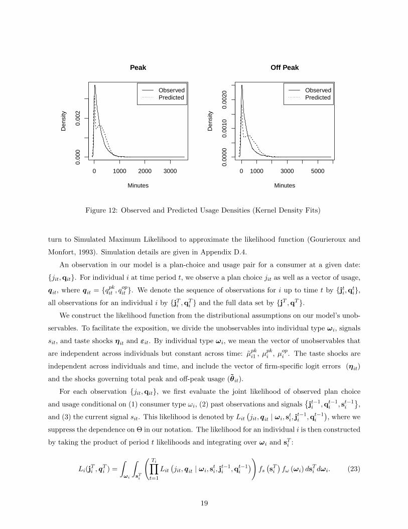
In Figure 12, we plot observed and predicted usage densities for both peak and off peak usage. The
model tries to fit the shape of the usage distribution as closely as it can, but the censored normal
specification we use produces a hump near zero that is not replicated in the data. A more flexible
usage specification, such as a mixture of normals, might fit the observed data better.
Table 14: Plan Shares for Initial Choices (percent)
October 2002 October 2003Plan 0 Plan 1 Plan 2 Plan 3 Plan 0 Plan 1 Plan 2 Plan 3
Observed 67 10 21 2 18 72 8 1Predicted 62 7 30 0.7 11 73 15 1
D.2 Simplified Likelihood Formulation
We begin this section by describing the structure of the likelihood function which arises from our
model. To simplify the exposition, we initially make several simplifying assumptions. In particular,
we ignore for the moment in-network and 8:00 pm to 10:00 pm usage shares, censoring of θit, and the
fact that the set of firms considered by i (Fit) is unobserved. Additional details about the likelihood
function, including censoring of θkit, a treatment of in-network calling, 8:00 pm to 10:00pm calling,
and quitting, are in Appendix D.3. As discussed below, the likelihood function for our model does
not have a closed form expression due to the presence of unobserved heterogeneity. We therefore
18
0 1000 2000 3000
0.00
00.
002
Peak
Minutes
Den
sity
ObservedPredicted
0 1000 3000 5000
0.00
000.
0010
0.00
20
Off Peak
Minutes
Den
sity
ObservedPredicted
Figure 12: Observed and Predicted Usage Densities (Kernel Density Fits)
turn to Simulated Maximum Likelihood to approximate the likelihood function (Gourieroux and
Monfort, 1993). Simulation details are given in Appendix D.4.
An observation in our model is a plan-choice and usage pair for a consumer at a given date:
{jit,qit}. For individual i at time period t, we observe a plan choice jit as well as a vector of usage,
qit, where qit = {qpkit , qopit }. We denote the sequence of observations for i up to time t by {jti,qti},
all observations for an individual i by {jTi ,qTi } and the full data set by {jT ,qT }.
We construct the likelihood function from the distributional assumptions on our model’s unob-
servables. To facilitate the exposition, we divide the unobservables into individual type ωi, signals
sit, and taste shocks ηit and εit. By individual type ωi, we mean the vector of unobservables that
are independent across individuals but constant across time: µpki1 , µpki , µopi . The taste shocks are
independent across individuals and time, and include the vector of firm-specific logit errors (ηit)
and the shocks governing total peak and off-peak usage (θit).
For each observation {jit,qit}, we first evaluate the joint likelihood of observed plan choice
and usage conditional on (1) consumer type ωi, (2) past observations and signals{jt−1i ,qt−1
i , st−1i
},
and (3) the current signal sit. This likelihood is denoted by Lit(jit, qit | ωi, sti, j
t−1i ,qt−1
i
), where we
suppress the dependence on Θ in our notation. The likelihood for an individual i is then constructed
by taking the product of period t likelihoods and integrating over ωi and sTi :
Li(jTi , q
Ti ) =
∫ωi
∫sTi
(Ti∏t=1
Lit(jit, qit | ωi, sti, jt−1
i ,qt−1i
))fs(sTi)fω (ωi) ds
Ti dωi. (23)
19

As it has no closed form solution, we approximate the integral over ωi and sTi in equation (23)
using Monte Carlo Simulation. For each individual, we take NS draws on the random effects from
fω(ωi) and fs(sTi)
and approximate the likelihood using
Li(Θ) =1
NS
NS∑b=1
(Ti∏t=1
Lit(jit, qit | ωib, stib, jt−1
i ,qt−1i
)). (24)
The simulated model log-likelihood is the sum of the logarithms of the individual simulated likeli-
hoods:
LL(Θ) =I∑i=1
log(Li(Θ)). (25)
We use NS = 400 (randomly shuffled) Sobol simulation draws to calculate the simulated log-
likelihood LL(Θ) (see Appendix D.4 for details).
D.2.1 Conditional period t likelihood
We now construct the period t likelihood that enters equation (23). For convenience, we reexpress
this likelihood conditional on the individual’s peak type µpki and her information set =it, which
includes past choices jt−1i and qt−1
i , signals to date sti, and all elements of type ωi excluding µpki .
Our construction follows naturally from the distributional assumptions on the taste shocks ηit and
θit.
For a customer who quits, we only observe that jit ∈ Jit\Jit,university and thus we sum:
Pr(quitit | µpki ,=it) =∑
jit∈Jit\Jit,university Pit(jit | =it). Otherwise, conditional on {µpki ,=it}, the
likelihood of an observation {jit,qit} is the product of the plan choice probability and the likelihood
of observed usage conditional on plan choice. In particular, conditional on sit, we will infer θit from
observed qit and write the likelihood as:
Lit(jit, qit | ωi, sti, jt−1
i ,qt−1i
)= Lit(jit, qit | µ
pki ,=it) = Pr(jit | =it)fq(qit|jit, µ
pki ,=it). (26)
Usage likelihood: First, we consider the likelihood of the observed usage qit. We know that
for k ∈ {pk, op}: qkit = θkitq(vkit(jit,=it)). Therefore, conditional on vkit(jit,=it), we can infer θkit from
usage: θkit(qkit, v
kit(jit,=it)) = qkit/q(v
kit(jit,=it)). Then, the joint normal assumption on εit and sit
leads directly to the distribution of θit conditional on sit: θit ∼ N(µkit + E [εit | sit] , V [εit | sit]
)(See Appendix B.3). Assuming no censoring (so that θit = θit) this yields the usage likelihood:
fq(qit|jit, µpki ,=it) = fθ|s(θit(qit,v
∗it (jit,=it)) | µi, sit)
∣∣∣∣∂θit(qit,v∗it (jit,=it)∂qit
∣∣∣∣ , (27)
20

where the term |∂θit(qit,v∗it (jit,=it) /∂qit| is the Jacobian determinant of the transformation be-
tween θit and qit (conditional on v∗it (jit,=it)). The usage likelihood must be adjusted whenever
an element of θit is censored at zero, and in the complete model there are additional terms to
incorporate data on in-network calling and 8-10pm calling (Appendix D.3).
Plan Choice Probability: Next we consider plan choice conditional on =it and an active
choice, which is denoted by conditioning on “C”. Let Fit denote the set of firms considered by the
consumer, Jit (f) denote the set of plans available from firm f ∈ Fit, and f (jit) denote the firm
which offers plan jit. (Note that Jit (f) depends on ji,t−1 because consumers can always keep their
existing plan.) Then the probability of choosing plan jit equals the probability of choosing firm
f (jit) multiplied by the probability of choosing plan jit conditional on choosing firm f (jit):
Pr (jit | C;=it, Fit) = Pr (f (jit) | C;=it, Fit) Pr (jit | C;=it, f (jit))
Conditional on an active choice, our assumption of firm-specific logit errors gives rise to the
following firm choice probability:
Pr(f | C;=it, Fit) =exp(maxk∈Jit(f) {Uitk(=it)})∑
g∈Fit exp(maxk∈Jit(g) {Uitk(=it)}).
Conditional on an active choice of firm f (jit), the probability of choosing plan jit is simply equal
to an indicator function specifying whether or not plan jit offered the highest expected utility to
consumer i of any plan offered by firm f (jit):
Pr (jit | C;=it, f (jit)) = 1
{Uitj(=it) = max
k∈Jit(f(jit)){Uitk(=it)}
}. (28)
(Typically we characterize Pr (jit | C;=it, f (jit)) by numerically computing bounds sit and sit such
that it is equal to 1 if an only if sit ∈ [sit, sit].)
In period 1, every consumer makes an active choice from the set of university plans, so Pr (ji1 | =i1) =
Pr (ji1 | C;=i1, f (ji1)). In every later period, however, consumers keep their existing plan ji,t−1
with probability (1− PC) and otherwise choose between the university, the outside option, and one
of three outside firms. Thus, unconditional on an active choice, the probabilities that an existing
customer switches to plan j 6= ji,t−1 in period t (where j could be the outside good) or keeps the
existing plan j = ji,t−1 are PC Pr (jit | C;=it, Fit) and PC Pr (jit | C;=it, Fit)+(1−PC) respectively:
Pr (jit | =it, Fit) =
PC Pr (jit | C;=it, Fit) if j 6= ji,t−1
PC Pr (jit | C;=it, Fit) + (1− PC) if j = ji,t−1
. (29)
21

Finally, the set of firms considered by consumers is unobserved. Each existing consumers
considers university plans, the outside option, and one of the three outside firms offering local
plans (AT&T, Cingular, or Verizon). Depending on the identity of the outside firm, there are three
possible consideration sets: Fit ∈{F 1it, F
2it, F
3it
}, each of which is equally likely. Thus the final plan
choice probability is:
Pr (jit | =it) =1
3
3∑k=1
Pr(jit | =it, F kit
). (30)
D.3 Complete Likelihood Formulation
In this section we revise the likelihood function described in Appendix D.2 to fully account for (1)
censoring of taste shocks θit, (2) free in-network calling and in-network calling data, and (3) near
9pm calling data.
There are three changes that affect the individual i likelihood, for which equation (23) gives
the simplified version. First, the type vector ωi is expanded to include parameters governing i’s
distribution of near 9pm and in-network usage: ωi = (µpki1 , µpki , µ
opi , α
pk,9i , αpk,ini , αop,ini ). Second,
the usage vector qit is expanded to include in-network and near 9pm calling data:
qit = {qpk,init , qpk,outit , qpk,9it , qop,init , qop,outit , qop,9it }.
Third, censoring of the latent taste shocks means that there is an additional vector of unobservable
variables. Let θ−i be the vector of all latent taste shocks for individual i that are negative and hence
unobserved (each corresponding to an observed θkit = 0). Let θ−,ti be the subset of θ
−i realized at
or before time t.
As before, we will construct the joint likelihood {jit,qit} by conditioning on {µpki ,=it}. Without
censoring, this was equivalent to conditioning on{ωi, j
t−1i ,qt−1
i , sti}
. Now, however, it requires also
conditioning on θ−,t−1i because consumer i’s information set =it includes all elements of θ
−i realized
before time t but these cannot be inferred from qt−1i . Thus we must now integrate out over this
additional unobserved heterogeneity:
Li(jTi , q
Ti ) =
∫ωi
∫sTi
∫θ−i
(Ti∏t=1
Lit
(jit, qit | ωi, sti, θ
−,t−1i , jt−1
i ,qt−1i
))(31)
fθ
(θ−i |sTi ,ωi, θ
−i ≤ 0
)fs(sTi)fω (ωi) dθ
−i ds
Ti dωi.
The expression for the likelihood Lit(jit, qit | µpki ,=it) given by equation (26) must also be
22

revised. In particular, we replace the density of qit, fq, with the likelihood of qit, lq:
Lit(jit, qit | µpki ,=it) = Pit(jit | =it)lq(qit|jit, µ
pki ,=it). (32)
The remainder of this section is devoted to fully specifying the likelihood of observed usage,
lq(qit|jit, µpki ,=it).
The usage vector qit is a function of the random variables θit and rit = {rpk,init , rop,init , rpk,9it , rop,9it }.
To compute the likelihood lq(qit | jit, µpki ,=it), we compute the likelihood of θit, l
θ(θit | jit, µpki ,=it)
and the likelihood of rit, lr(rit | jit,=it), put them together and then do the change of variables
from these variables to qit:
lq(qit | jit, µpki ,=it) = lθ(θit|jit, µpki ,=it)l
r(rit|jit,=it)∣∣∣∣det
(∂ (θit, rit)
∂qit
)∣∣∣∣ .Below we (1) outline the construction of lθ(θit|jit, µpki ,=it) which accounts for censoring, (2) outline
the construction of lr(rit|jit,=it) by incorporating (a) in-network calling data, and (b) near 9-pm
calling data, and (3) finish by outlining |det (∂ (θit, rit) /∂qit)| for the change of variables.
D.3.1 Censoring
Conditional on µi and sit, the taste shock θit follows a bivariate normal distribution:
θit ∼ N(µkit + E [εit | sit] , V [εit | sit]
)where E [εit | sit] and V [εit | sit] follow from Bayes rule in Appendix B.3 equations (15)-(16). We
denote the joint density by fθ|s(θit|µi, sit), and the marginal density of θkit for k ∈ {pk, op} by
fkθ|s(θ
kit|µki , sit).
As described in Section V, θkit can be inferred from observed usage. If θkit > 0, then this gives
the value of the latent variable: θkit = θkit. If θkit = 0, however, we can only infer that θ
kit ≤ 0. When
θit is not censored, its likelihood is simply fθ|s(θit(qit,v∗it (jit,=it)). Otherwise, the likelihood of
θit(qit,v∗it (jit,=it) must be adjusted by substituting the probability that θ
kit is censored for fθ|s:
lθ(θit | jit, µpki ,=it) =
fθ|s(θit|µi, sit) if θpkit > 0, θopit > 0
Pr(θpkit ≤ 0|µpki , sit, θ
opit )fk
θ|s(θopit |µ
opi , sit) if θpkit = 0, θopit > 0
Pr(θopit ≤ 0|µopi , sit, θ
pkit )fk
θ|s(θpkit |µ
pki , sit) if θpkit > 0, θopit = 0
Pr(θpkit ≤ 0, θ
opit ≤ 0|µi, sit) if θpkit = 0, θopit = 0
, (33)
23

where θit’s dependence on qit and v∗it (jit,=it) is suppressed from the notation. We then use the
change of variables formula to arrive at the likelihood of qit (rather than θit) We leave this step,
however, until after considering in-network and near-9pm calling.
D.3.2 In-network and Near-9pm Calling
By including data on whether calls are in or out of network and whether calls are within 60
minutes of 9pm, the usage vector becomes qit = {qpk,init , qpk,outit , qpk,9it , qop,init , qop,outit , qop,9it }, where
“in”, “out”, and “9” signify in-network, out-of-network, and near-9pm calling respectively. As
before, qpkit = qpk,init + qpk,outit and qopit = qop,init + qop,outit denote total peak and total off-peak calling
respectively. In this section we discuss three issues related to handling in-network calling: (1) a
data limitation, (2) the inference of θit, and (3) an additional term in the likelihood.
(1) Data Limitation: We always observe total peak and off-peak calling because we observe
the time and date of all calls. An important data limitation, however, is that call logs only directly
identify outgoing calls as in-network or out-of-network. This information provides lower and upper
bounds on in-network calling: qk,init
and qk,init for k ∈ {pk, op}. The lower bound on total in-network
usage is simply the total outgoing in-network minutes we observe. The upper bound is outgoing
in-network minutes plus all incoming minutes. Analogous bounds on out-of-network usage are
qk,outit
= qkit − qk,init and qk,outit = qkit − qk,init
for k ∈ {pk, op}. Fortunately, the network status of plan
0 peak calls (and off-peak calls for plan 0 that did not include free off-peak) can be inferred from
whether they were charged 11 cents or 0 cents per minute. Thus, precisely when in-network calls
are differentially priced, we can infer qpk,init and qop,init exactly.
(2) Inferring θit: The fact that in-network and out-of-network calling may be priced differently
complicates our inference of θit from usage data. For k ∈ {pk, op}, θkit is calculated by equation
(34) if category k calls are not priced differentially by network status or by equation (35) if category
k calls are priced differentially by network status:
θkit = qkit/q(vkit), (34)
θkit = qk,init /q(vk,init ) + qk,outit /q(vk,outit ). (35)
There is always sufficient information to infer θit from usage conditional on the threshold vector
v∗it (jit,=it) because qk,init and qk,outit are observed precisely when equation (35) applies.
(3) Likelihood Function: Next we turn to the likelihood of in-network and near 9pm calling
24

shares.4 For k ∈ {pk, op}, if in-network usage is observed exactly then we can calculate the exact
share of category k calling opportunities that are in-network as
rk,init =qk,init /q(vk,init )
qk,init /q(vk,init ) + qk,outit /q(vk,outit ),
and the exact share of category k calling opportunities that are near-9pm as
rk,9it = qk,9it /qk,outit .
For k ∈ {pk-in,pk-9,op-in,op-9}, as rkit follows a censored-normal distribution, where the under-
lying normal distribution is defined by αki + ekit, we can write the likelihood of rkit as:
fk(rkit|αki ) =
Φ(−αki /σke) if rkit = 0
φ((rkit − αki )/σke)/σke if rkit ∈ (0, 1)
1− Φ((1− αki )/σke) if rkit = 1
.
For k ∈ {pk, op}, if we only observe bounds on qk,init and qk,outit then we can only calculate bounds
for rk,init and rk,9it :
rk,init ∈
[qk,init
θkitq(vk,init )
,qk,init
θkitq(vk,init )
]=[rk,init , rk,init
],
rk,9it ∈
[qk,9it
qk,outit
,qk,9it
qk,outit
]=[rk,9it , r
k,9it
].
Note that qk,9it ≤ qk,outit
, so qk,9it > 0 implies the bounds on rk,9it are within [0, 1]. For k ∈ {pk, op},
if the upper bound on the category k in-network usage share is below one (rk,init < 1) then the
likelihood for the bounds on rk,init and rk,9it are as follows.
lk,in(rk,init , rk,init | αki ) =
fk(rk,init |α
k,ini ) if rk,init = rk,init = rk,init
Φ((rk,init − αk,ini
)/σk,ine
)− Φ
((rk,init − αk,ini
)/σk,ine
)if 0 < rk,init < rk,init < 1
Φ((rk,init − αk,ini
)/σk,ine
)if 0 = rk,init < rk,init < 1
4Note that, for k ∈ {pk, op}, when qkit = 0 we have no information about the share of in-network usage rk,init andwhen qk,outit = 0 and we have no information about the share of near-9pm rk,9it .
25

lk,9(rk,9it , rk,9it | α
k,9i ) =
fk,9(rk,9it |αk,9i ) if rk,9it = rk,9it = rk,9it
Φ((rk,9it − α
k,9i
)/σk,9e
)− Φ
((rk,9it − α
k,9i
)/σk,9e
)if 0 < rk,9it < rk,9it < 1
Φ((rk,9it − α
k,9i
)/σk,9e
)if 0 = rk,9it < rk,9it < 1
1− Φ((rk,9it − α
k,9i
)/σk,9e
)if 0 ≤ rk,9it < rk,9it = 1
Moreover, in the case rk,init < 1, the likelihoods of rk,init and rk,9it are independent and we can write
the joint likelihood as the product of lk,in(rkit, rkit | αki ) and lk,9(rk,9it , r
k,9it | α
k,9i ).
When rk,init = 1, constructing the likelihood of rk,init and rk,9it is more complicated. The com-
plication stems from the way that bounds on in-network and out-of-network calls are constructed.
The lower bound on out-of-network calls is the total number of outgoing calls to out-of-network
numbers, plus (if in-network calling is free) the total number of non-free minutes used after an
overage occurs. If this lower bound is zero, then total outgoing-calls to landlines were also zero.
Total landline calls near 9pm could be zero for two reasons: rk,init = 1, or rk,9it = 0. If the upper
bound on rk,init binds, then rk,9it could take any value. However, if the upper bound on rk,init does
not bind, then rk,9it must be zero. Following this logic, the joint likelihood of rk,init ≤ rk,init ≤ 1 and
rk,9it ∈ [0, 1] is
lr,k(rk,init , rk,init = 1, rk,9it ∈ [0, 1] | αk,ini , αk,9i
)
=
1− Φ((1− αk,ini )/σk,ine )
+ Φ(−αk,9i /σk,9e )
Φ((1− αk,ini )/σk,ine )
−Φ((rk,init − αk,ini )/σk,ine )
if rk,init > 0
1− Φ((1− αk,ini )/σk,ine ) + Φ(−αk,9i /σk,9e )Φ((1− αk,ini )/σk,ine ) if rk,init = 0.
Thus the joint likelihood of in-network and near-9pm calling opportunity shares for category
k ∈ {pk, op} is
lr,k(rk,init , rk,init , rk,9it , rk,9it | α
k,ini , αk,9i ) =
lr,k(rk,init , rk,init | αk,ini ) · lk,9(rk,9it , rk,9it | α
k,9i ) if rk,init < 1
lr,k(rk,init , rk,init = 1, rk,9it ∈ [0, 1] | αk,ini , αk,9i ) if rk,init = 1.
Finally,
lr(rit|jit,=it) = Πk∈{pk,op}lr,k(rk,init , rk,init , rk,9it , r
k,9it | α
k,ini , αk,9i ).
In the following section we perform the change of variables transformation to write the likelihood
as a function of qit rather than rit.
26

D.3.3 Change of Variables
The joint likelihood of θit and rit will be the product of the lθ and lr. This is not the likelihood of
the observed usage vector qit, however, because qit is a function of θit and rit and we need to make
the change of variables between them. Summarizing what we’ve outlined above, the transformation
from the data to θk, rk,in, rk,9 for k ∈ {pk, op} is
θk =qk,out
q(vk,out)+
qk,in
q(vk,in); rk,in =
qk,out
qk,out + qk,in q(vk,out)
q(vk,in)
; rk,9 =qk,9
qk,out.
We need to take the Jacobian determinant of this transformation and multiply it by each
likelihood observation. We note that the Jacobian we take depends on what we observe. Below,
we describe the case where all the six different q’s are observed. The Jacobian is simpler if less
data is observed. For example, if only θk were observed, and we could not compute the r’s, we
would only take the Jacobian of the transformation between θkit and qkit for k ∈ {pk, op}. Defining
y = (qpk,out, qpk,in, qpk,9, qop,out, qop,in, qop,9) and x = (θpk, rpk,in, rpk,9, θop, rop,in, rop,9),
f(y) = f(x)
∣∣∣∣det
(∂x
∂y
)∣∣∣∣ .For k ∈ {pk, op}, the derivatives we need are: ∂θk/∂qk,out = 1/q(vk,out), ∂θk/∂qk,in = 1/q(vk,in),
∂rk,9/∂qk,out = −qk,9(qk,out)−2, ∂rk,9/∂qk,9 = 1/qk,out,
∂θk
∂qk,9=∂rk,in
∂qk,9=
∂rk,9
∂qk,in= 0,
and
∂rk,in
∂qk,out= qk,in
q(vk,out)
q(vk,in)
(qk,out + qk,in
q(vk,out)
q(vk,in)
)−2
∂rk,in
∂qk,in= −qk,out q(v
k,out)
q(vk,in)
(qk,out + qk,in
q(vk,out)
q(vk,in)
)−2
.
27

Then the Jacobian of the transformation that maps y into x is:
∂θpk
∂qpk,out∂θpk
∂qpk,in0 0 0 0
∂rpk,in
∂qpk,out∂rpk,9
∂qpk,in0 0 0 0
∂rpk,9
∂qpk,out0 ∂rpk,9
∂qpk,90 0 0
0 0 0 ∂θop
∂qop,out∂θop
∂qop,in0
0 0 0 ∂rop,in
∂qop,out∂rop,in
∂qop,in0
0 0 0 ∂rop,9
∂qop,out 0 ∂rop,9
∂qop,9
.
The determinant of this Jacobian will be
det
(∂x
∂y
)=
∏k∈pk,op
(∂θk
∂qk,out∂rk,in
∂qk,in∂rk,9
∂qk,9− ∂θk
∂qk,in∂rk,in
∂qk,out∂rk,9
∂qk,9
).
D.4 Simulation Details
In this section we describe in detail the procedure we follow for approximating integrals in the
likelihood using Monte Carlo Simulation.
D.4.1 Simulation Draws
It is well-known that the value of Θ which maximizes the simulated log-likelihood LL is inconsistent
for a fixed number of simulation draws NS due to the logarithmic transformation in equation (25).
However, it is consistent if NS →∞ as I →∞, as discussed in Hajivassiliou and Ruud (1994).
We chose NS = 400; to arrive at this value we conducted some simple artificial data experiments
where we simulated our model and attempted to recover the parameters, finding that 400 draws was
sufficient to recover the true parameter draws to roughly 5 percent accuracy. We found that 400
draws per consumer was the maximum number of draws we could feasibly include in our estimation.
We re-estimated our model with only 300 draws, and found that our parameter estimates were very
similar to those obtained with 400 draws, suggesting that increasing the number of draws beyond
400 would not significantly improve the parameter estimates.
We also found in our experiments that we were able to reduce simulation bias significantly by
using a deterministic Sobol sequence generator to create the random draws, rather than canonical
random number generators. (We randomly shuffle the Sobol draws, independently for each element).
Goettler and Shachar (2001) describe some of the advantages of this technique in detail. We use
the algorithm provided in the R package randtoolbox to create the draws (Dutang and Savicky,
2010).
28

D.4.2 Approximate Likelihood Function
As it has no closed form solution, we approximate the integral over ωi, sTi , and θ−i in equation
(31) numerically using importance sampling and Monte Carlo Simulation. A natural first approach
would be to take NS draws on the random effects from fθ
(θ−i |sTi ,ωi, θ
−i ≤ 0
), fω(ωi), and fs
(sTi)
and approximate individual i’s likelihood using
Li(Θ) =1
NS
NS∑b=1
(Ti∏t=1
Lit
(jit, qit | ωib, stib, θ
−,t−1ib , Fitb, j
t−1i ,qt−1
i
)),
where b indexes the simulation draw. Unfortunately, this approach would lead the approximate
likelihood function to be discontinuous. (This fact follows from equation (28) because Pr(jit | C;=it,
f (jit)) is discontinuous in sit.)
Our alternate approach is to compute the bounds sit and sit such that Pr(jit | C;=it, f (jit)) = 1
if an only if sit ∈ [sit, sit]. (We discuss computation of the bounds in detail in the following section.)
We then take NS draws on sit from a truncated normal within these bounds. Drawing sit from
the truncated density fs(s)/Pr (sit ∈ [sit, sit]) necessitates multiplying the likelihood expression
Lit by Pr (sit ∈ [sit, sit]) to cancel out the denominator when one takes the expectation of the
approximation. Thus our approximate likelihood function is:
Li(Θ) =1
NS
NS∑b=1
(Ti∏t=1
Lit
(jit, qit | ωib, stib, θ
−,t−1ib , Fitb, j
t−1i ,qt−1
i
)Pr (sit ∈ [sit, sit])
), (36)
which is continuous. Given the bounds [sit, sit], drawing sit from a truncated normal distribution
can be accomplished easily through importance sampling. (For an overview see Train (2009) pages
210-211.)
Integrating over ωi is straightforward as we can simply draw ωi from its normal distribution
given Θ. We draw censored values θkit < 0 period by period. If peak usage is censored and off-peak
usage is positive, we draw θpkit,b from fθ,2(θ
pkit,b | θ
pkit,b < 0, θ
opit,b,µi,b), where the density fθ,2 represents
the truncated univariate normal density of θpkit conditional on θopit , prior period usage and simulated
draws. The case when only off-peak usage is censored is symmetric. When both peak and off peak
usage are zero, we draw both θpkit and θopit from a truncated bivariate normal distribution. As for
sit we draw from truncated normal distributions via importance sampling.
Note that we write Lit conditional on a simulated draw of the firm consideration set, Fitb.
We do so because we substitute the conditional plan choice probability Pr (jit | =it, Fitb) evaluated
at a randomly drawn Fitb ∈{F 1it, F
2it, F
3it
}in place of the unconditional plan choice probability
Pr (jit | =it) from equation (30) when calculating Lit from equation (32) at a particular simulation
29

draw b. This approach reduces computation time because it means that we only have to compute
the expected utility for a third of outside firm plans at each simulation draw.
D.4.3 Computing Bounds
We now turn to the computation of the bounds [sit, sit] from which we draw simulated values of
sit. First consider the case in which all plans in i’s choice set include free off-peak calling. In this
case only the consumer’s beliefs about θpkit and rin,pkit (rather than also those about θopit and rin,opit )
affect plan expected utility. Let µpkθit = E[θpkit | sit] and (σpkθt )2 = V [θ
pkit | sit], for which formulas
are given in Appendix B.3. Our approach is to first calculate bounds on µpkθit that are implied by
plan choice jit, and then invert µpkθit = µpkit + ρs,pkσpkε sit, to find corresponding bounds on sit. In
particular, µpkθit ∈ [µθit, µθit] implies that
µθit− µpkit
σpkε ρs,pk≤ sit ≤
µθit − µpkit
σpkε ρs,pk. (37)
Expected utility for a plan with free off-peak calling varies across individuals and time depending
on the three parameters {µpkθ,it, σpkθt , α
pki }. To calculate the bounds µpkθit ∈ [µ
θit, µθit], we begin by
calculating expected utility of each university plan on a three dimensional grid of µpkθ,it, σpkθt , and
αpki values. (This computation occurs only once, prior to evaluating the likelihood.) The µθ,it grid
is regular between -100 and 1200 minutes, and each point is spaced 10 minutes apart. The σ2θ,t grid
is irregular, where the grid points are {σ2θ,1, ..., σ
2θ,T }. The αpki grid has 11 equally spaced points
between 0 and 1.
Next, for each consumer i and period t, we fix σpkθt and a simulated αpkib and (using linear
interpolation between adjacent αpki grid points) compute expected university plan utilities over a
one dimensional grid of µpkθ,it values. At each µpkθ,it value on the grid, we determine the optimal
university plan. Then bounds on µθ,it implied by observed plan choice jit are computed using
linear interpolation. For example, if plan 0 is chosen, and plan 0 is optimal for all µθ,it grid points
{1, ..., k}, and plan 1 is optimal for point k+1, then we assume that the upper bound on µθ,it occurs
where the interpolated utilities cross for plans 0 and 1 in between points k and k + 1.5 Bounds on
signals immediately follow: [sit, sit] =(
[µθit, µθit]− µ
pkit
)/(σpkε ρs,pk
).
The preceding algorithm works when off-peak calling is free. At some dates, however, plan 0
charges 11 cents per minute off-peak as well as on peak. We refer to this pricing as the costly
5We did experiment with finding where actual utilities crossed, rather than interpolated utilities, in a simplifiedversion of the model where we estimated beliefs from period 1 choices in the fall of 2002. We found that estimatedbeliefs were the same for each method, but the interpolation was much faster.
30

version of plan 0. The expected utility of costly plan 0 varies across individuals and time due
to variation in {µopθ,it, αopi } as well as {µpkθ,it, σ
pkθt , α
pki }. (The parameter σopθ is constant across time
because there is no learning about off-peak type.) To account for this variation, we calculate the
difference in expected utility between free-off peak calling and 11 cent per minute off-peak calling
on a two dimensional grid of {µopθ,it, αopi } values.
Next, we notice that for a particular i and t, µopθ,it is a function of µpkθ,it:
µopθ,it = µopi + ρs,opσopε sit = µopi + σopε
ρs,opρs,pk
(µpkθ,it − µ
pkit
).
Therefore, for each i and t we can compute (via linear interpolation) the expected utility of the
costly version of plan 0 over a grid of µpkθ,it values, conditional on σpkθt and simulated values αpkib and
αopib . We then compute bounds as before.
Finally, note that the bounds sit and sit are functions of the time t plan choice jit and information
set =itb (excluding sitb). In particular, period t bounds depend on the previous period’s signal si,t−1,b
and latent taste shock θpki,t−1,b (via their effect on µpkθ,it). Therefore we must first draw signals st−1
ib
and censored shocks θ−,t−1ib in order to compute bounds sit and sit and draw a signal sitb.
D.5 Computational Procedures
When we compute our standard errors, each time we run our estimator on a different subsampled
data set we also use a different set of pseudo random draws to compute the log likelihood function.
Our standard errors will therefore also account for simulation error.
We wrote the program to evaluate the likelihood in R and Fortran. The evaluation of the like-
lihood is computationally intensive for two reasons: first, it must be evaluated at many simulation
draws; second, for each choice a consumer could make, at each time period and each draw, we often
must solve for v∗it and α9,opi using a nonlinear equation solver. Our estimation method therefore
falls into an inner-loop outer-loop framework, where the inner loop is the solution of the v∗it’s and
α9,opi ’s, and the outer loop maximizes the likelihood.
We summarize the algorithm for computing these variables in four steps. Step 1 is to compute
αop,9i,b conditional on the simulated draws and the other model parameters. Recall that we assume
that a consumer’s average taste for weekday-evening landline-usage is the same thirty minutes
before and after 9pm. For each consumer i and each simulation draw b, we compute αop,9i,b as the
solution to equation (22) in Appendix C, which extends equation (9) to account for in-network
calling. As this equation does not have an analytic solution, we compute αop,9i,b with a nonlinear
equation solver. The result of this step is used to compute the structural error for rop,9it .
31

The next three steps compute the calling threshold vector v∗it,b and θit,b period-by-period.
Because the v∗it,b is a function of past values of θit,b through the Bayesian learning, these three
steps are iterated across both individuals i, and time periods t. Step 2 calculates consumer beliefs
about θit,s in two parts following Section III.D. First, consumer beliefs about µpki , (µpkit,b, σ2it) are
updated via Bayes rule. Second, beliefs about θit,b are computed from (µpkit,b, σ2it) and µopi,b. (No
updating is required for t = 1.) In step 3 we calculate v∗it,b following it’s characterization in
Appendix C, which depends on the beliefs calculated in step 2. Recall that components of v∗it are
either known to be 0 cents or 11 cents or must be calculated by numerically solving a first-order
condition (either equation (20) or (21) which are the extensions to equation (4) that account for
in-network calling given in Appendix C). In step 4, we calculate θit,b. When θit,b is not censored,
we can compute θit,b from observed usage conditional on β and v∗it,b using equations (34)-(35) in
Appendix C. When censoring occurs, we use the simulated value for θit,b.
With αop,9i,b , θit,b and v∗it,b in hand we can compute the choice probabilities and the density
of observed usage in equation (23). Choice probabilities are calculated from consumer expected
utilities, Uitj,b, which are defined in equation (19) for all plans in consumers’ choice sets. These
depend on plan-specific calling threshold vectors v∗itj,b (which are all computed as part of the vector
v∗it,b). Next, notice that
V(q(vkitj , x
kit), x
kit
)= xkit
1
βq(vkitj)
(1− 1
2q(vkitj)
)(38)
is linear in xkit for k ∈ {pk-out, pk-in, op-out, op-in} and hence∑
k V (qkit, xkit) is linear in θpkit and
θopit . Thus E[∑
k V (qkit, xkit)]
can be computed analytically (up to evaluation of the standard normal
cumulative distribution). Moreover, the expected price E [P (q)] is a linear function of the expected
amount θpkit exceeds Qijt/q(vpkitj,b) (or xpk,outit exceeds Qijt/q(v
pk,outitj,b ) for free-in-network), which we
can also evaluate analytically in all cases except for when plan 2 offers free in-network minutes. In
the latter case we approximate the expectation with Gaussian quadrature.
We optimize our likelihood in two steps. The first step uses a Nelder-Mead optimizer to get
close to the optimum. From there we use a Newton-Raphson optimizer to reach the optimum
within a tighter tolerance. Because the optimization algorithms will stop at local optima, it is
important to have good starting points. To arrive at starting points for the model, we choose the
usage parameters (the means and variances of the µ’s, α’s, and ε’s) and the β to match observed
usage.6 Conditional on these choices of usage parameters, we choose initial belief parameters to
6We assume that vpkitj is equal to 3 cents for plan 3, 5 cents for plan 2, and 8 cents for plan 1, and maximize
32

match the observed plan shares. To do so, we use our model to simulate plan shares for the 2002
to 2003 school year and the 2003 to 2004 school year, and match those simulated shares to the
observed shares during these two years. We chose to split the data in that way to exploit the fact
that plan 0 stopped offering free off-peak minutes at the beginning of the 2003 to 2004 school year.
E Equilibrium Price Calculation
To compute the pricing equilibrium we begin with 1,000 simulated consumers who we assume are
in the market for T = 12 periods, and 3 identical firms offering 3 plans (we assume that 4 plans are
offered in the calibration). In period 1, simulated consumers choose from the set of all plans offered
by any of the three firms. In later periods, the consumer chooses between the plans offered by
the firm they chose in period t− 1, those offered by a randomly assigned alternative firm, and the
outside option, consistent with the model we estimate. We denote the firm’s fixed cost of serving
a customer as FC and the marginal cost of providing peak minutes as c (off-peak minutes are
assumed to have zero marginal cost).
We solve for a symmetric equilibrium by iterating on firm best response functions: we start by
assuming all firms offer a set of plans that looks close to what is offered in the data, and compute
one firm’s best response to that using a numerical optimizer. We then assume that all firms offer
the best response plans, and compute the best response to those plans. The algorithm converges
when the difference in prices between one best response and the next are below a threshold (we
take the average percentage change in the characteristics and use a tolerance of 1 percent).
The remainder of this section provides details on how the best responses are calculated. For
t > 1, a simulated consumer i is assigned a vector of draws on the type, signals, tastes, firm
errors, and plan consideration (ωi, si,θi,ηi,PCi). In the first period, however, for each possible
plan choice we draw a signal conditional on being inside bounds corresponding to that plan choice
and then integrate over the firm logit error ηf to compute a choice probability for the plan. This
different treatment in the first period reduces the discontinuities in the simulated profit function
that arise from simulating firm errors ηi1 and a single signal si1. Moreover, doing this only for
t = 1 avoids the computational problem that the number of possible plan choice vectors {ji1, ..., jiT }
increases exponentially with T .
the likelihood of usage conditional on those guesses at vpkitj . We chose those values of vpkitj because they matched the
average values of vpkitj that were produced by simulating the model at parameters which were in the neighborhood of
the estimates. We stress that we only use the guesses at vpkitj to arrive at starting points; we solve for the endogenous
vpkitj ’s when running the full simulated maximum likelihood.
33

Our approach is to begin by solving for prices for the T = 1 equilibrium. This is a smooth
problem for which we use a derivative-based BFGS optimizer. We then solve the T = 12 problem
using the solution for the T = 1 problem as a starting point. This is not a smooth problem and
hence we use a simplex optimizer to solve for the best response.
During optimization we put constraints on the plan characteristics the firm can offer. For all
plans j offered by the same firm, the constraints are:
Mj ≥ 0; Mj ≥Mj−1
Qj ≥ 0; Qj ≥ Qj−1
0 ≤ pj ≤ p; pj ≤ pj−1.
These constraints ensure we produce plans that look like what we observe in the data. Typically
we find an interior solution so the constraints do not bind - exceptions to this are the upper bound
p on overage rates without bill-shock regulation and the lower bound Qj ≥ 0 when we de-bias
consumers. To ensure the optimizer does not wander into bad areas of the parameter space, we
take a penalty function approach.
F Calibration Exercise
As discussed in Section VII, to run our endogenous-price counter-factual simulations we first cali-
brate the logit-error weight 1/λ and the marginal cost of providing a peak call, c. For the exercise
and all the counterfactuals we assume that the fixed cost of serving a customer, FC, is $15.00. Our
algorithm for the calibration is as follows: First, we limit the analysis to publicly available prices,
which means that we focus on the price offerings of the three firms AT&T, Cingular, and Verizon.
(Sprint did not offer any local plans, so we did not include them.) Second, we draw 1000 simulated
consumers and simulate their usage and plan choices for one year. We assume that the three firms
each offer menus of four three-part tariffs and play a symmetric Nash equilibrium. Finally, we
solve for equilibrium prices and compare them to prices observed over the two year period. When
computing equlibrium prices, we restrict included minute allowances, Qj , to weakly increase with
fixed fees, Mj , and bound overage rates pj ≤ 50¢. Formally, firm j offers k = 1, .., 4 plans, where
the plans are ordered according to their fixed fees, and we denote the predicted price schedule as
a function of λ and c as (Mjk(λ, c), pjk(λ, c), Qjk(λ, c)) and the observed price schedule of a firm
during month t as (Mjkt, pjkt, Qjkt). We choose λ and c to minimize the squared difference between
34

observed and predicted prices:
{λ, c} = arg minλ,c
∑j,k,t
((Mjk(λ, c)−Mjkt)
2 + (pjk(λ, c)− pjkt)2 + (Qjk(λ, c)−Qjkt)2)
.
This calibration exercise yields λ = 0.03 and c = 0.02. We used a grid search to find the optimal λ
and c.
After the calibration we tested how sensitive our parameter estimates from our primary speci-
fication (λ = 1) differed for two alternate specifications, 1) a specification which fixed O = 0 and
let λ be free, and 2) a specification where λ was fixed to its calibrated value of 0.03 and the rest
of the parameters were free. Specification 1) yielded a value of λ of roughly 0.06. Apart from λ,
the difference between the estimated parameters in the primary specification and the alternatives
were negligible. (To make sure the small differences were not due to an optimization issue we redid
the estimations with several different step sizes, ranging from large to very small. The optimizer
converged to the same estimates for all step sizes we chose.)
G Robustness
G.1 Overage Rate
A natural concern is that our results will be sensitive to the bound we impose on the overage rate
since that effects how far overage rates fall when bill-shock regulation is imposed. To address this
issue, Table 15 reports simulations with $0.35 and $0.75 overage rate caps. (For context, empirically
observed overage rates range from $0.35 to $0.50 in our sample period.) We find that our results
are robust to the alternative overage rate limits.
The intuition for robustness is as follows: First, profits are unaffected by the maximum overage
rate as fixed fees adjust in equilibrium to compensate. Second, average usage varies by less than
10 minutes per month between $0.35 and $0.75 caps because (1) overconfidence diminishes the
effect of the overage rate on calling thresholds, and (2) minute allowances adjust in equilibrium in
an off-setting manner. Third, social surplus changes little because calling changes little. Fourth,
consumer surplus changes little because it is the difference between two stable quantities, social
surplus and profits.
G.2 Learning
Columns 4 and 5 of Table 5 show that our predictions about the consequences of bill-shock regula-
tion depend importantly on estimated biases. A natural question, then, is how much the predictions
35
Table 15: Effect of Bill-Shock Regulation for Different Overage Rate Caps
Overage rate cap: 50 cent cap 35 cent cap 75 cent capRegulation: None Bill shock None Bill shock None Bill shock
(1) (2) (3) (4) (5) (6)
Plan 1 M 42.88 39.28 46.85 39.28 37.18 39.28Q 216 0 188 0 225 0p 0.50 0.17 0.35 0.17 0.75 0.17Share 39 26 36 26 35 26
Plan 2 M 48.64 50.66 52.73 50.66 41.33 50.66Q 383 80 365 80 363 80p 0.50 0.12 0.35 0.12 0.75 0.12Share 38 23 36 23 40 23
Plan 3 M 58.12 68.23 60.82 68.23 50.98 68.23Q 623 540 613 540 576 540p 0.50 0.12 0.35 0.12 0.75 0.12Share 14 40 17 39 17 39
Outside good share 10 12 11 12 9 12
Usage 240 239 245 240 236 240Overage revenue 223 152 178 153 294 153
Annual profit 501 509 501 508 508 508Annual consumer welfare 903 870 911 884 916 884Annual total welfare 1404 1379 1413 1393 1424 1393∆ Annual profit 7 7 1∆ Annual consumer welfare -33 -27 -32∆ Annual total welfare -26 -20 -31
All welfare and profit numbers are expressed in dollars per customer per year. We simulate 10,000 consumersfor 12 months.
36

would change if time passes allowing consumer beliefs to evolve via learning but all else remains
equal. To answer this question, we ran our bill-shock counterfactual simulation after allowing con-
sumers beliefs to evolve for either 12 months or 36 months before making their first plan choice.
Results are shown in Table 16. One would expect the magnitude of welfare changes in response
to bill-shock regulation to decline with learning as we have already shown that they disappear
completely with de-biasing. This is what we find. Predicted annual consumer surplus losses from
bill-shock regulation decline from $33 in our primary counterfactual to $27 with 12 months pre-
learning and to $12 with 36 months pre-learning. The qualitative prediction that average consumer
surplus falls a small amount is robust. The most notable difference in pricing is that the plan
menu collapses to two plans with bill-shock regulation given additional learning. This response
to additional learning makes sense because our main specification already shows that de-biasing
reduces the menu to two tariffs.
G.3 Price Sensitivity
As noted in footnote 27, one might be concerned that our estimate of β is biased. On the one hand,
our estimate of β might be too high if (in contrast to our assumption) some of the increase in usage
at 9pm occurs because consumers delay calls until after 9pm. On the other hand, our estimate of β
is much smaller than what would be estimated from the jump in usage at 9pm alone. We therefore
perform sensitivity analysis constraining β to alternative values.
To save computational time, we use a half-sample of the data. Table 17 reports estimated
parameters from three specifications. Specification (1) estimates our full model on the half-sample.
The estimate of β is 2.86, slightly higher than the estimate on the full sample of 2.70. Specification
(2) holds fixed β at half its estimated value and re-estimates the other 27 parameters. Likewise,
specification (3) holds fixed β at 1.5 times its estimated value and re-estimates the other 27 pa-
rameters. (Note that these alternative values of β lie more than 2 standard errors away from our
estimate. Thus they are meaningfully different values.)
As expected, many parameters are stable across the three specifications. For instance, off-peak
parameters, in-network calling parameters, near-9pm calling parameters, the plan consideration
probability PC , overconfidence δ, and correlations ρs,pk, ρµ, ρµ,op, and ρε, are all stable. Addition-
ally, if one uses the standard errors estimated in the main specification as a baseline, all but µop for
the large value of β are within 2 standard deviations of the baseline estimates. Also as expected,
other parameters vary monotonically with β in reassuring ways. As β increases, larger values of θ
are required to explain the same usage when marginal price is positive. Thus it is reassuring that
µpk0 , σpkµ , σpkε , and µpk0 increase with β. (In contrast it is not surprising that µop0 and other off-peak
37
Table 16: Effect of Bill-Shock Regulation After 12 or 36 Months of Consumer Learning
Learning: None 12 months 36 monthsRegulation: None Bill shock None Bill shock None Bill shock
(1) (2) (3) (4) (5) (6)
Plan 1 M 42.88 39.28 42.6 49.16 43.98 58.05Q 216 0 204 97 207 280p 0.50 0.17 0.50 0.15 0.50 0.16Share 39 26 22 40 19 56
Plan 2 M 48.64 50.66 45.81 63.91 47.12 63.14Q 383 80 331 441 323 478p 0.50 0.12 0.50 0.15 0.50 0.16Share 38 23 43 48 38 31
Plan 3 M 58.12 68.23 51.94 52Q 623 540 497 479p 0.50 0.12 0.50 0.50Share 14 40 25 33
Outside good share 10 12 10 12 10 13
Usage 240 239 247 245 253 261Overage revenue 223 152 215 102 199 65
Annual profit 501 509 485 481 483 471Annual consumer welfare 903 870 948 921 955 943Annual total welfare 1404 1379 1432 1402 1438 1414∆ Annual profit 7 -3 -12∆ Annual consumer welfare -33 -27 -12∆ Annual total welfare -26 -30 -24
All welfare and profit numbers are expressed in dollars per customer per year. We simulate 10,000 consumerslearning for 12 or 36 months to generate initial beliefs, followed by 12 months of plan and usage choices forpricing and welfare calculations.
38
Table 17: Parameter Estimates at Different β Values
Est. β Low β (−50%) High β (+50%)Parameter (1) (2) (3)
β 2.86 1.43 4.29
µpk0 219.97 205.28 274.99
µpk0 273.69 257.51 311.76µop0 402.48 406.94 417.24
σpkµ 195.51 168.67 202.73
σpkµ 146.98 160.32 160.07σopµ 431.71 453.14 425.8ρµ,pk 0.22 0.43 0.17
ρµ,op 0.01 0.01 0.01
ρµ 0.59 0.62 0.66
σpkε 254.76 230.55 296.01σopε 344.08 340.91 351.04ρε 0.54 0.53 0.54ρs,pk 0.45 0.43 0.44
δ 0.36 0.36 0.37
µpk,9α -0.01 -0.01 -0.01
σpk,9α 0.06 0.06 0.06
σpk,9e 0.11 0.12 0.11
σop,9e 0.12 0.12 0.12PC 0.06 0.06 0.06O 1.16 1.83 0.84
µpkα 0.33 0.36 0.31µopα 0.39 0.4 0.39
σpkα 0.18 0.18 0.18σopα 0.17 0.17 0.17
σpke 0.18 0.19 0.18σope 0.17 0.17 0.16δr 0 0 0
b1 -53.72 -52.23 -36.78b2 0.84 0.59 0.87
Log-likelihood 142680 142733 142763
Estimation uses a half-sample of the data.
39

parameters do not increase with β as off-peak usage is typically free and independent of β.)
Several parameters are worth commenting on in more detail. Aggregate mean bias b1 appears
stable to reducing β but declines in absolute value for larger β (although it is still negative). Inter-
estingly, the correlation ρµ,pk declines with β which means (following equation (8) that conditional
mean bias b2 increases with β. Thus if we have overestimated β we may also have slightly over-
estimated conditional mean bias. The intuition for this effect is that large plan choice is correlated
with high usage. As β increases, the model attributes more of this difference to the price effect
and less to the selection of high users into large plans. The model turns down self-selection by
reducing the correlation between true types and point estimates so that consumers’ plan choices
are increasingly noisy.
Next we conduct our counterfactual simulation of the effect of bill-shock regulation at estimates
corresponding to the three different values of β. These are reported in Table 18. First note that
the outside good is smaller and more stable under regulation at lower values of β, which makes
sense since the value of phone service relative to the outside good is higher at lower β. Second note
that overage rates fall more with regulation when β is higher, which again makes sense because
larger marginal price cuts are needed for more price sensitive consumers. Third, included minute
allowances increase with β for similar reasons. Fourth, usage increases with β. This might first
sound surprising, that more price sensitive consumers consume more. However, note that the change
in usage depends both on varying β and the accompanying changes in the parameters governing
the distribution of θ. Since the estimates are all trying to fit the same usage levels for the same
prices in the demand data we should expect that at equal prices usage would not vary with the
specifications. So it should actually not be a surprise that usage increases when marginal price
decreases at larger β values.
Turning to the welfare predictions, our result that consumer surplus and social welfare on
average decrease by a small amount is robust for different values of β. For some values of β we find
profits increase and at others we find profits decrease. This finding is partially (but not completely)
explained by the fact that at higher β the outside good is a closer substitute and firms have less
market power to raise fixed fees following regulation. More generally, it may reflect that fact that
the regulation does not have a strong direct effect on market power and hence there is not a clear
prediction a priori about whether profits should go up or down.
G.4 Heterogeneity
As our sample consists entirely of students a possible concern is that our sample is more homo-
geneous and more or less price sensitive than the general population. To diagnose whether this
40
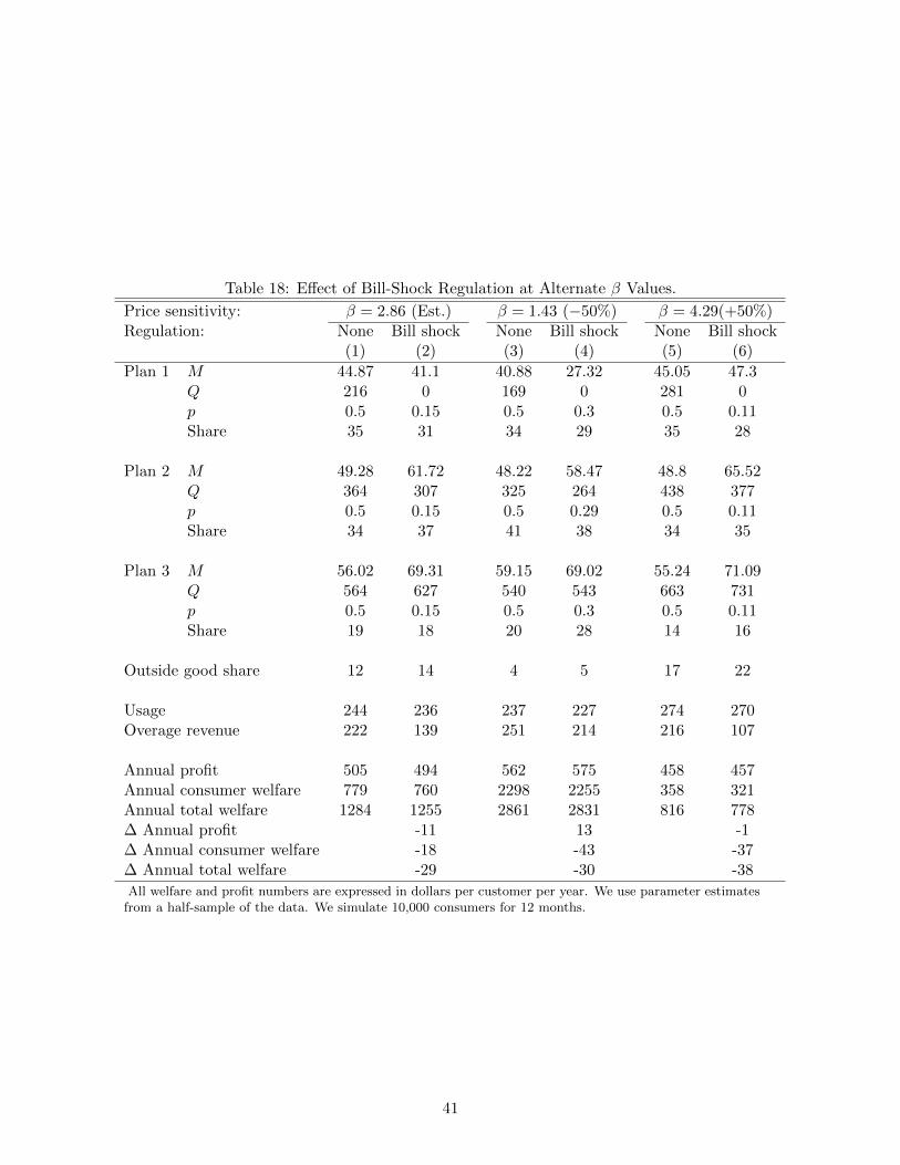
Table 18: Effect of Bill-Shock Regulation at Alternate β Values.
Price sensitivity: β = 2.86 (Est.) β = 1.43 (−50%) β = 4.29(+50%)Regulation: None Bill shock None Bill shock None Bill shock
(1) (2) (3) (4) (5) (6)
Plan 1 M 44.87 41.1 40.88 27.32 45.05 47.3Q 216 0 169 0 281 0p 0.5 0.15 0.5 0.3 0.5 0.11Share 35 31 34 29 35 28
Plan 2 M 49.28 61.72 48.22 58.47 48.8 65.52Q 364 307 325 264 438 377p 0.5 0.15 0.5 0.29 0.5 0.11Share 34 37 41 38 34 35
Plan 3 M 56.02 69.31 59.15 69.02 55.24 71.09Q 564 627 540 543 663 731p 0.5 0.15 0.5 0.3 0.5 0.11Share 19 18 20 28 14 16
Outside good share 12 14 4 5 17 22
Usage 244 236 237 227 274 270Overage revenue 222 139 251 214 216 107
Annual profit 505 494 562 575 458 457Annual consumer welfare 779 760 2298 2255 358 321Annual total welfare 1284 1255 2861 2831 816 778∆ Annual profit -11 13 -1∆ Annual consumer welfare -18 -43 -37∆ Annual total welfare -29 -30 -38
All welfare and profit numbers are expressed in dollars per customer per year. We use parameter estimatesfrom a half-sample of the data. We simulate 10,000 consumers for 12 months.
41

may be true, we use our data to estimate a version of Jiang’s (2013) model adapted to our data.
Comparison of the resulting estimates to those reported in Jiang (2013) that are based on national
data suggest that students in our sample may indeed be more homogeneous and less price sensitive
than the general population. (Details of this exercise following in Appendix H.)
We therefore conduct a sensitivity analysis to the variance of the joint normal distribution of
consumer type {µpki1 , µpki , µ
opi } in conjunction with higher values of β. We perform our bill shock
exercise with two modified sets of estimates. In one set of estimates we scale up σpkµ by 2 and set
β = 4, and in the second we scale σpkµ up by 2.5 and set β to 1.5 times its estimated value. To
preserve the biases, we rescale σpkµ by the same factor as σpkµ , and keep all the model’s correlation
parameters the same (so the covariances are also multiplied by 2 or 2.5, depending on the alternative
specification). The results of this exercise are shown in columns 3 through 6 of Table 19 (columns
1 and 2 replicate columns 1 and 3 of Table 5 in the main body of the paper, showing the predicted
impact of bill shock regulation using our estimated parameters).
Without bill shock, both fixed fees and the number of included minutes in a plan increase as
the variance of µpki and the price coefficient rises. As the variance in the population rises there are
more consumers who place a high value on talking, which likely explains both the rise in fixed fees
and the number of included minutes. Similarly, there are more consumers who place a low value
on talking, which likely explains the rise in the share of the outside good. The larger shares of the
outside good also reflect higher values of β.
The impact of bill-shock regulation on prices is similar to what we find in the main counter-
factual: fixed fees rise (except for plan 1), the number of included minutes drops, and the overage
rates drop. Turning to the welfare effects of the counterfactuals, they are similar in that consumer
welfare drops, and total welfare drops. One difference relative to our main results is that firm
profits also drop, which is likely a result of higher consumer price sensitivity. In conclusion, we
believe this exercise suggests that the qualitative implications of our paper would be unchanged if
our sample was more heterogeneous and more price sensitive.
H Replication of Jiang’s (2013) Model Using Our Data
In this section we estimate Jiang’s (2013) model on our data. We attempt to follow Jiang’s (2013)
approach as closely as possible, given the differences between our two datasets. The version of
Jiang’s (2013) model that we estimate has 7 parameters: we estimate the population average of
the taste parameter (θi), the standard deviation of the taste parameter, the standard deviation of
the perception error (ω), an overage price coefficient, a fixed-fee price coefficient, and two dummy
42
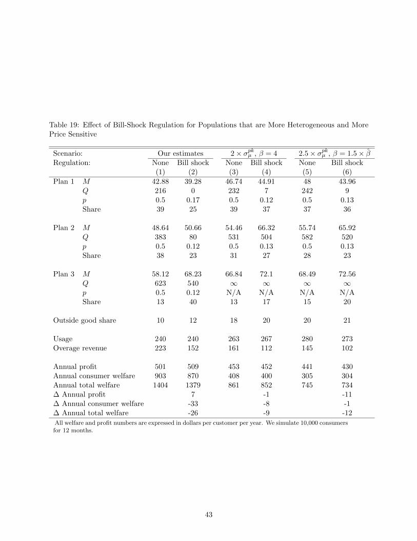
Table 19: Effect of Bill-Shock Regulation for Populations that are More Heterogeneous and MorePrice Sensitive
Scenario: Our estimates 2× σpkµ , β = 4 2.5× σpkµ , β = 1.5× βRegulation: None Bill shock None Bill shock None Bill shock
(1) (2) (3) (4) (5) (6)
Plan 1 M 42.88 39.28 46.74 44.91 48 43.96Q 216 0 232 7 242 9p 0.5 0.17 0.5 0.12 0.5 0.13Share 39 25 39 37 37 36
Plan 2 M 48.64 50.66 54.46 66.32 55.74 65.92Q 383 80 531 504 582 520p 0.5 0.12 0.5 0.13 0.5 0.13Share 38 23 31 27 28 23
Plan 3 M 58.12 68.23 66.84 72.1 68.49 72.56Q 623 540 ∞ ∞ ∞ ∞p 0.5 0.12 N/A N/A N/A N/AShare 13 40 13 17 15 20
Outside good share 10 12 18 20 20 21
Usage 240 240 263 267 280 273Overage revenue 223 152 161 112 145 102
Annual profit 501 509 453 452 441 430Annual consumer welfare 903 870 408 400 305 304Annual total welfare 1404 1379 861 852 745 734∆ Annual profit 7 -1 -11∆ Annual consumer welfare -33 -8 -1∆ Annual total welfare -26 -9 -12
All welfare and profit numbers are expressed in dollars per customer per year. We simulate 10,000 consumersfor 12 months.
43

variables for plan characteristics - whether a plan includes free off-peak and whether a plan included
free in-network. The last two parameters were included to ensure our approach is as comparable
as possible to Jiang’s (2013) model, which also includes dummy variables for plan characteristics
(although the included characteristics such as free long-distance and free roaming indicators are
different than ours). Jiang (2013) also includes demographic interactions in the price coefficients
that we cannot include because we do not have demographic information. However, her demo-
graphic variables are quite coarse and it may be sufficient to assume they are zero for our sample
- they include a dummy variable for whether an individual is in a family, a dummy for whether
the individual is high-income, and a dummy for whether the individual is over 55 or not. Jiang’s
(2013) estimates of the demographic interactions are not statistically significant. Jiang (2013) also
estimates the variance of the logit error in her specification. We found we could not identify the
logit error variance in our specification so we fixed the standard deviation of the logit error to the
value she estimates - 66.94. We assume that consumers are rational, as Jiang (2013) does, and
restrict the mean of the perception error to be 1.
Following Jiang (2013) we estimate the model parameters using method of moments.7 Our
moment selection follows hers very closely. We break our sample up into 9 periods (our period
definitions correspond to the periods outlined in Appendix A Table 6; we drop the initial period
8/02-10/02 where plan 0 was unavailable), and choose parameters to match the following moments:
1. Share of plan j in period t.
2. Average probability of being 10 percent below or 10 percent above the number of included
minutes in period t (for 3 part tariffs only).
3. Average usage in period t.
4. Coefficient of variation in usage in period t.
5. Correlation between usage and overage rate in period t.
We construct our moments using only the first observed bill for each consumer because Jiang’s
(2013) model does not incorporate plan switching or grandfathering of plans, and because we
believe that Jiang’s (2013) sample selection procedure will oversample new customers. In terms of
weighting, moments are weighted according to 1) the standard deviation of the outcome variable,
7It would not in fact be possible to estimate Jiang’s (2013) model using maximum likelihood because Jiang’s(2013) model assumes that all consumers use a strictly positive number of minutes every month. Her model wouldpredict zero likelihood for observations in our data where we observe zero usage.
44
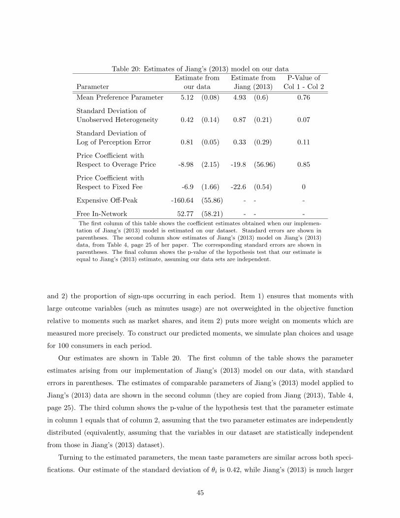
Table 20: Estimates of Jiang’s (2013) model on our dataEstimate from Estimate from P-Value of
Parameter our data Jiang (2013) Col 1 - Col 2
Mean Preference Parameter 5.12 (0.08) 4.93 (0.6) 0.76
Standard Deviation ofUnobserved Heterogeneity 0.42 (0.14) 0.87 (0.21) 0.07
Standard Deviation ofLog of Perception Error 0.81 (0.05) 0.33 (0.29) 0.11
Price Coefficient withRespect to Overage Price -8.98 (2.15) -19.8 (56.96) 0.85
Price Coefficient withRespect to Fixed Fee -6.9 (1.66) -22.6 (0.54) 0
Expensive Off-Peak -160.64 (55.86) - - -
Free In-Network 52.77 (58.21) - - -
The first column of this table shows the coefficient estimates obtained when our implemen-tation of Jiang’s (2013) model is estimated on our dataset. Standard errors are shown inparentheses. The second column show estimates of Jiang’s (2013) model on Jiang’s (2013)data, from Table 4, page 25 of her paper. The corresponding standard errors are shown inparentheses. The final column shows the p-value of the hypothesis test that our estimate isequal to Jiang’s (2013) estimate, assuming our data sets are independent.
and 2) the proportion of sign-ups occurring in each period. Item 1) ensures that moments with
large outcome variables (such as minutes usage) are not overweighted in the objective function
relative to moments such as market shares, and item 2) puts more weight on moments which are
measured more precisely. To construct our predicted moments, we simulate plan choices and usage
for 100 consumers in each period.
Our estimates are shown in Table 20. The first column of the table shows the parameter
estimates arising from our implementation of Jiang’s (2013) model on our data, with standard
errors in parentheses. The estimates of comparable parameters of Jiang’s (2013) model applied to
Jiang’s (2013) data are shown in the second column (they are copied from Jiang (2013), Table 4,
page 25). The third column shows the p-value of the hypothesis test that the parameter estimate
in column 1 equals that of column 2, assuming that the two parameter estimates are independently
distributed (equivalently, assuming that the variables in our dataset are statistically independent
from those in Jiang’s (2013) dataset).
Turning to the estimated parameters, the mean taste parameters are similar across both speci-
fications. Our estimate of the standard deviation of θi is 0.42, while Jiang’s (2013) is much larger
45

at 0.87. If we interpret differences in the parameter estimates due to differences in the samples
used for estimation (as opposed to differences in specification, or model implementation), then the
estimates suggest that our sample is more homogenous than Jiang’s (2013) sample, which is unsur-
prising since our sample consists of students while hers is drawn from the general population. This
conclusion must be tempered somewhat due to the large standard error in Jiang’s (2013) estimate
of the standard deviation of θi - as shown in the third column of the table the two parameters are
not statistically different at the 5 percent level. Our estimate of the perception error variance is
0.81, which is more than twice Jiang’s (2013) estimate of 0.33. Again, the standard error around
her estimate of this standard deviation is 0.29, indicating that our estimate is not statistically dif-
ferent than hers. Turning to the overage price coefficient, our estimate is much smaller than Jiang’s
(2013) estimate. However, the standard error around Jiang’s (2013) estimate of this coefficient is
extremely large at 57, so our estimate of the price coefficient is not statistically different from hers.
The only parameter that is statistically different from Jiang’s (2013) is the price coefficient on the
overage price, which is around one third the magnitude. This suggests that our sample is less price
sensitive than Jiang’s (2013) sample which is reasonable - students likely come from higher income
families relative to the general population so it makes sense they would be less sensitive to prices.
We next turn to the question of how our bill-shock counterfactual might be affected if the
estimates from the model presented in the body of the paper are biased in a manner that is similar
to the differences we observe between the two parameter estimates in Table 20. Because the two
models are very different this exercise is imperfect. For example, there is no counterpart to the
perception error in the model in our paper, so it is not clear to us what the implications of having
a larger perception error variance are. Similarly, as Jiang’s (2013) dataset is a cross-section there
is no counterpart to our εpkit . However, we can make guesses at how the estimated distribution
of unobserved heterogeneity in tastes and the price coefficient might change. Jiang’s (2013) θi
parameter, which determines unobserved heterogeneity in taste for calling, functions similarly to
our µpki . Our estimates of Jiang’s (2013) model in Table 20 imply an average θi of 183 minutes, while
Jiang’s (2013) imply an average θi of 202 minutes. Since the average tastes are about the same,
we do not think we would get substantially different estimates of the average µpki were we to apply
our model to her data. The estimated standard deviation of θi from our implementation of Jiang’s
(2013) model is about 80 minutes, while Jiang’s (2013) estimate is 215 minutes. This suggests we
would get a larger estimate of the variance of µpki were we to apply our model to her data. If
we underestimate the standard deviation of µpki by the same proportion as we underestimate the
standard deviation of θi, we would want to increase the standard deviation of µpki by about 2.5
times.
46

Our estimates in Table 20 also imply that we underestimate consumer price sensitivity. One way
to get a sense of how much we underestimate price sensitivity is to consider how much a consumer
who observes a price increase from 0 to 11 cents on a two part tariff would reduce her usage for
each set of estimates. In Jiang’s (2013) model, a consumer’s target usage on a two part tariff has
a closed form solution:
x∗ =θi
aip+ 1
Our estimates of Jiang’s (2013) model imply an average consumer would target usage at 183
minutes if the marginal price were 0, and 92 minutes if the marginal price were 11 cents - a 50
percent reduction in usage. Jiang’s (2013) estimates imply an average consumer would target 202
minutes at a price of 0, and 64 minutes at a marginal price of 11 cents - a 68 percent reduction
in usage. If our model underestimates the actual reduction in usage by 18 percent, then the price
coefficient would have to be a little over 4. This analysis motivates our choice of robustness checks
in Appendix G.4 Table 19.
47

References
Borenstein, Severin, “To What Electricity Price Do Consumers Respond? Residential Demand Elastic-
ity Under Increasing-Block Pricing,” 2009. http://faculty.haas.berkeley.edu/borenste/download/
NBER_SI_2009.pdf.
DeGroot, Morris H., Optimal Statistical Decisions, New York: McGraw-Hill, 1970.
Dutang, Christophe and Petr Savicky, “randtoolbox: Generating and Testing Random Numbers.,”
2010. R package version 1.1. http://cran.r-project.org/web/packages/randtoolbox/.
Goettler, Ronald L. and Ron Shachar, “Spatial Competition in the Network Television Industry,” The
RAND Journal of Economics, Winter 2001, 32 (4), 624–656.
Gourieroux, Christian and Alain Monfort, “Simulation-based inference : A survey with special refer-
ence to panel data models,” Journal of Econometrics, 1993, 59 (1-2), 5–33.
Hajivassiliou, Vassilis A. and Paul A. Ruud, “Classical Estimation Methods for LDV Models Us-
ing Simulation,” in R.F. Engle and Daniel L. McFadden, eds., Handbook of Econometrics, Volume IV,
Amsterdam: North-Holland, 1994.
Jiang, Lai, “The Welfare Effects of ‘Bill Shock’ Regulation in Mobile Telecommunication Markets,” Novem-
ber 2013. http://www.lai-jiang.com/uploads/Jiang_JobMarketPaper.pdf.
Roodman, David, “How to do xtabond2: An introduction to difference and system GMM in Stata,” Stata
Journal, 2009, 9 (1), 86–136.
TelcoData.us, “npa-nxx-companytype-ocn.csv,” 2005. Telecommunications Database. https://www.
telcodata.us/data-downloads (accessed October 13, 2005).
Train, Kenneth E., Discrete Choice Methods with Simulation, 2nd ed., New York: Cambridge University
Press, 2009.
48