Com plex Systems 3 (1989) 383-405

Cellular Automaton Model for F luid Flow in PorousMedia

Paul PapatzacosHegsko leseutetet j Rogaland, Postboks 2557, Ullandhaug,

4001 Stavanger, Norway

Abstract . A cellular automaton model for the simulation of fluidflow in porous media is presented. A lattice and a set of rules areint roduced, such th at the flow equations in the continuum limit areformally the same as the equations for one-phase liquid flow in porousmedia. The model is valid in two as well as th ree dimensions. Numer­ical calculatio ns of some simple problems are presented and comparedwith known analytical results. Agreement is within estim ated error s.

1. Introdu ction

It is well known that the Navier-Stokes equation can be deri ved by twoalternative methods, which may be called macroscopic and microscopic. Themacroscopic me thod builds on the hypothesis that fluid s are structurelesscontinua and uses conservation laws of general validity [6]. The viscositycoefficients are introduced as constants to be determined by experiments.T he microscopic approach, on the other hand, is based on the molecularstructure of fluids and uses the framework of statistical physics [8]. Theviscosity is here calcu lable in terms of the intermolecular potent ial.

T here is an analogous division in the theory of flow in porous mediaand the Darcy equation . The macroscopic point of view st arts with Darcy 'slaw, which states that the rate of one-dimensional flow is proportional tothe pressure gradient, and generalizes this law by introducing a permeabili tyte nsor. T he components of this tensor are to be determined by experiments.T he microscopic me thod is represented by an extensive literature (see forexample [9] and refere nces given there) where it is shown that the Darcyequat ion ari ses from an averaging ou t of Navier-Stokes flow by the poresand that the permeability te nsor is in principle deducible from the poregeome try. The length scale is here microscopic only as far as the porousme dium is concerned: the pores are visible but the fluid is struct ureless .

The recent paper by Rothman [7] on the cellular automaton simulationof flow in po rous media is in t he microscopic tradition. Using the FHP [3]triangular-lattice gas it shows how to estimate the permeability of almost

© 1989 Comp lex Systems Publications , Inc.

384 Paul Papatzacos

arbit rary pore geometries by introducing impermeable reg ions in the lat ti ce.It is thus a fram ework for st udying permeab ility.

The prese nt paper is in th e macroscopi c tradition. A lat tice and a setof ru les are devised in such a way that the result ing lat ti ce gas obeys anequation which is formally identical to the equat ion of motion of one ph aseflow in porous media. The coefficients of the latt ice-gas equat ion of motionar e adjustable so that one is ab le to match the corresponding coefficientsof t he equat ion to solve. T his model is thus a framework for the numer icalsolut ion of a specific equation . T he motivation for such a mo del is that someimportan t problems are difficult to solve, eit her analytically or by standardnumerical methods. Irr egular boundari es, impermeable layers, large perme­ability cont ras ts be tween adjacent layers are some of the features of suchproblems.

Secti on 2 presents the equation governing one phase flow in porous me­dia , which is the equation to simulate. The lattice-gas (lattice and rul es) ispr esen ted in section 3. The calculations lead ing to the flow equation for thelat tice gas, following the met hods that hav e bee n used for simulating hydro­dynamics [3,4,10], are shown in sections 4 and 5. Finally, sect ions 6 and 7present numerical checks.

2 . One phase flow in porous m edia

The differential equation for liquid flow at constant temperature in a porousmedium [1J is essentially a mass conservation equation

(2. 1)

where 8; and 8: denote partial derivation wit h respect to t ime if an d co­ordinate x;(i = 1, 2, 3). The summation convent ion is assum ed and primedletters are used for those qu antities which will eventually be scaled, reserv ingunprimed let ters to their dimensionless counterparts to be introduced lateron . S is the mass of fluid , injected (if positive) or removed (if negative) perunit time and per unit volume of the medium. Further , ep is the rock poros­ity, r/ is the fluid mas s per unit volume, and qi are the components of theso-called superficial or Darc y velocity, given by

(2.2)

Here II is the fluid viscosity, p is the fluid pressure, J{ij is the permeabili tytensor, and gj is the acceleration du e to gravity with components (0, - g , 0) ifthe second coordinate-axis is vertical and points upwards. (Such a placementof coordinate axes is convenient for the presentation of the rest of the paper.See sect ion 3.)

Cellular A utomaton Model for Fluid Flow in Porous Media 385

For liquid flow at constant te mperature one usually assumes [1] that r/ isa function of pressure exclusively and that the compressibility

1 dr/(J= -­r/ dp

(2.3)

is a constant.Equations (2.1-2.3) are usually combined into one equat ion for the pres­

sur e [l J. From the point of view of a cellu lar automaton simulation it is mor einterest ing to have r/ as the depend ent variable. With the ass umption thatr/ = r/(p) and using equation (2.3) one gets

8jr/ = (Jr/ojP,

and combining this with equations (2.1) and (2.2) one obtains

o;r/ - ( tp/-l(J)- l ](ijo:(8jP - (J r/ gj ) = se:' ,

(2.4)

(2.5)

assuming that ](ij, tp, u, and (J are constants. The following assumptionsabout the pe rmeability tensor usually allow one to model most cases of prac­t ical interest. It is symmet ric, one of its principal axes is vertical , and it isisotropic in the hor izontal direction . The second axis being vertical , theseassumpt ions imply that

so that the flow equation , equation (2.5) , becomes

tp /-l(J8; r/ - kh(0~ 2 + 8~2 )r/ - kv8~ (8~ r/ + (Jgr/2) = /-l (JS . (2.6)

It is appropriate, at this po int, to scale t he pr ime d quantities by intr odu cinga length scale Lo, a t ime scale To and a density scale (}o:

x; = LOXi, t' = Tot,,

(} = (}o(}· (2.7)

T he dimensionless flow equat ion is then

where

(2.8)

N; = khTo/( tp /-l (JL6),

.Ng = g(}oLo(J ,

N; = kvTo / (tp /-l(JL6) ,

s; = STo/(tp(}o).(2.9)

The dimensionless form of Darcy's law , equat ions (2.2) , is

(Lo/To)-l tp-lqj = -N« (} -101 (},

(Lo/To) - l tp- l q2 = <N; ((}- 182(} + .Ng(J) ,

(Lo/To) - l tp- l q3 = -N« (}-103(} ,

(2.10)

386 Paul Papatzacos

where Lo/To has been used as a velocity scale, and where ep- 1qi is the inter­stitial velocity [I ]. It is reminded that interst iti al velocity plays the role, ina porous medium, of the usu al fluid velocity.

The orders of magnitude of the dime nsion less numbers defined by equa­tions (2.9) are very depend ent on the reservoir . The values given below forthe rock and fluid parameters are meant to fix ideas.

kh ::::; 10- 12 m 2 , kv/kh ::::; 10- 1 ,

f3 ::::; 1O- 9 Pa-1 , J-l ::::; 10- 3Pa s,

120 ::::; 103 kg m", g ::::; 10 m s- 2,ep ::::; 0.3, S ::::; 1 kgm- 3s- 1 ,

Lo ::::; 1m, To ::::; 1 s.

One then finds:

Nh ::::; 3, N; ::::; 3 X 10- 3 ,

(2.11)Ny ::::; 10- 5 , N, ::::; 3 X 10- 3 .

The purpose of this paper is to find a cellular automaton model for simulat ingequat ion (2.8).

3 . The lattice-gas rules

The lat tice considered is cubi c with grid length A. The time step is denotedT, and an elementary velocity c is introduced by

A = CT .

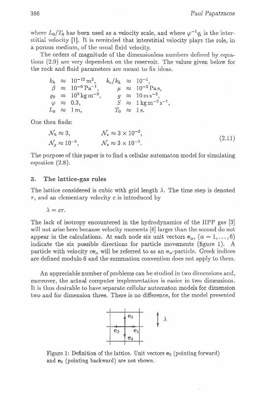
T he lack of isotropy encountered in the hydrodynamics of the HPP gas [3]will not arise here becaus e velocity moments [4J larger tha n the second do notappear in the calculat ions. At each node six unit vectors e", (a = 1, . . . , 6)indicat e the six possible dir ections for particl e movement s (figure 1). Apart icle with velocity ce; will be referred to as an e,,-p ar ticl e. Greek indicesare defined modulo 6 and the summation convent ion does not app ly to them.

An ap preciab le number of problems can be studied in two dimensions and,mor eover , the actual compute r imp lement ation is easier in two dimensions .It is thus desirabl e to have separ at e cellular au tomato n models for dimensiontwo and for dimension three. T here is no difference, for the model presented

Figure 1: Definition of the lattice. Unit vectors e 5 (pointing forward)and e6 (pointing backward ) are not shown.

Cellular A utomaton Model for Fluid Flow in Porous Media 387

here, between two and three dimensions, other than appending two extravectors to the two-dimensional case and ap plying the rules to these extravelocity dir ections. Since equation (2.8) shows that the vertical directi onplays a special role becau se of the effect of gravity, vectors e l to e4 will beconsidered to be in a ver tical plane, with e2 pointing upwards. In such amanner a two-dimensional model, obtained by dropping the two dir ecti onses and e6, will ret ain the possibili ty of reprodu cing different horizontal andvertical permeabilities and of simulating gravity effects. The pr esentation inthe rest of the paper is, as much as possible, independent of the number ofdimensions.

Particle movements are governed by the following three rul es.

1. There is at most one par ticle per state, where a state is specified bythe position and the velocity. Thus there are at most 2d par ticl es pe rlattice node, where d is the dimensi onality of the space (d = 2 or 3) .

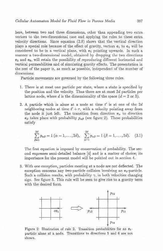
2. A particle which is alone at a node at time t' is at one of the 2dneighboring nodes at t ime i' + 'T" , with a velocity pointing away fromthe node it just left. The t ransit ion from dir ect ion e., to directione(3 t akes place with probability Pa(3 (see figure 2). These probabilitiessat isfy

2d

L P a (3 = 1 (Q' = 1, . . . , 2d),(3= 1

2d

L P a (3 = 1 ({3 = 1, . . . , 2d) .0'=1

(3.1)

The first equation is imposed by conservation of probability. T he sec­ond expresse s semi-detailed balance [4J and is a matter of choice; itsimportan ce for the present model will be pointed out in section 4.

3. With one except ion , particles meeting at a node are not deflected . Theexcept ion concern s any two-p article collision involving an eTparticle.Such a collision results, with probability" in both velocities changingsign . See figur e 3. T his rule will be seen to give rise to a gravi ty te rmwit h the des ired form.

m P

P12

13 Pn

P14

Figure 2: lllustration of rule 2. Transition probabilities for an el ­parti cle alone at a node. Transitions to directions 5 and 6 are notshown.

388 Paul Pepeizecos

Figure 3: illustration of rule 3. Any two-particle collision involvingan e2-particle results, with probability f, in an inversion of both ve­locities.

The rul es are seen to be consistent. They conserve particle number butnot momentum. An additional rule concerning particle creation or annihila­tion will be given in section 6.

4. The lattice Bolt zmann equations and their equil ibrium solu tion

Int roducing f ,,(r' ,t') , t he mean popula t ion at no de r ', time t' , and velocitydirection e" , the ru les can be translated into what Frisch et al. [4] call the"lattice Boltzmann equations." These equations are here written directlyand reference is made to [4] for their just ificat ion in terms of an ensemble av­erage, using the Boltzmann assumption, of a set of microdynamical equationsbetween Boolean variables. Keep ing in mind that the Boltzmann assumptionimplies that many-particle distribution functions are products of one-particledist ribution functions one find s:

where

2d

.o,,/II = L l {J (p{J" - 8{J,,) +"'d2 h",{J=1

(a = 1, ... , 2d),

(4.1)

(4.2)

are calculated at r ' and t'. The notation in equation (4.2) is as follows:

2d

II = II (1 - f ,,),,,= 1

(4.3)

and

13 - iI ,-iI - 13 - 15 - 16,16 - is.

(4.4)

If d = 2then 15 and 16 are dropped from the expressions for h2 and h4 •

Cellular Automaton Mo del for Fluid Flow in Porous Media 389

It is easy to check that, as a consequence of conservation of probability(see the first set of equations (3.1)) ,

(4.5)

(4.6)

which expresses particle conservation.Equation (4.1) is valid when r' is at a node and t' is a multiple of T . The

transition to a continuum description is done by assuming that t he fa haveappreciable variations only over a space scale L :::t> ), and a time scale T :::t> T

so that it is possible to interpolate between the discrete points at which thefa are originally defined. Actually one assumes that the interpolation givesfunctions that can be differentiated arbitrarily many times. The left -handside of equation (4.1) can then be rep laced by it s Taylor expansion, to yielda differential form of the lattice Boltzmann equation:

f= ~(TO: + ),eaiO:t fa = na .n = ! n.

The space and t ime vari ab les are now scaled with the above quantities LandT:

x;= LXi, t' = Tt, (4.7)

and it is assumed that

(4.8)

Since the purpose of the model is to describe diffusion effects, the time-scaleT must be such that [4]

T/ T = c2. (4.9)

Using equations (4.7-4.9) in equation (4.6) , the latter takes the followingdimensionless form:

Finally, fluid dens ity is defined by

2d

p(r, t) = L: fa (r, t ),a=!

(4.10)

(4.11)

while fluid momentum, which is not a conserved quantity, is not used .An equilibrium solution f~q is now looked for , such that na(f~q ) = 0,

in the form of an expansion in powers of c. This equilibrium solut ion willdepend on the one conserved quantity, p. It is assumed in the present modelthat the fluid density is at most of order e:

p = 2dc<p (4.12)

390 Paul Papatzacos

where the factor 2d is included for convenience. Equation (4.11) showsthat one may try f~q = ed : The expressions defin ing n" (equations (4.2­4.4)) show that, because of semi -detailed balance (the second set of equa­tions (3.1)), this expression of f~q is correct to order c. One can thus set

(4.13)

where, to satisfy equation (4.12),

(4.14)

(It will be seen later that terms of order c3 are not needed.) The X" arefound by solving equations n,,(f~q) = °perturbatively to order c2

• One findsthat the X" satisfy

2d

2:= X/3(P/3" - 8/3,,) = 2,(d -1)(8"2 - 8"4)¢>2 ./3=1

(4.15)

Because of equations (3.1) the matrix with elements P"/3 - 8,,/3 has rank2d - 1. There are thus 2d independent equations in the set consisting ofequations (4.14) and (4.15), which determines the 2d X" 's uniquely. Note thatthe hitherto unspecified matrix P"/3 must satisfy the condition that the rank ofP"/3 - 8,,/3 is 2d - 1. The opposite case is equivalent to the existence of spuriousconservation laws. The calculation of the x" is deferred to section 5.2, wherea special form for the matrix P"/3 is introduced.

5. The perturbation solution and the flow equation

5.1 The perturbation solution

Reference is made to [4J and [10J for a justification of the calculations whichnow follow. A solution to the differential Boltzmann equation (4.10) is soughtby perturbing around the equilibrium solution, i.e., by setting

and by requiring that the correction terms do not modify the density:

2d

2:= 1/J~1) = 0,,,=1

2d

2:= 1/J~2) = 0.,, =1

(5.1)

(5.2)

(5.3)

Cellular Automaton Model for Fluid Flow in Porous Media 391

Combining equat ions (4.13) and (5.1) one finds, for the left -hand side ofequation (4.10):

c;2 eaJJi(<p +1/Ji1) ) + C;3 [Ot(<p + 1/Ji1) )

+ eaiOi(Xa + 1/Ji2) ) + ~ eai eaAOj(<P + 1/Ji1

) ) ]

+ 0(C;4), (5.4)

where the terms of order C;4 involve terms in the expansion of f a which areof order C;3 (see equ ation (5.1)). To order e, the right-hand side of equa­t ion (4.10) is

2d

Da = e L 1/J~l ) (P(3a - o(3a) +0(C;2)./3=1

T his must vanish identically. Accounting for equat ions (5.2) and rememb er­ing that Pa(3 - oa(3 has rank 2d - 1, one then finds that

1/J~1 ) = o. (5.5)

With this simplification and usin g equ ation (4.15), the right -hand side ofequat ion (4.10) be comes, to order C;2,

2d

Da = C;2L 1/J~2 ) (P(3a - 0/3a ) + 0(C;3).(3=1

(5.6)

(5.7)

Equating this to the right-hand side of equation (5.4 ), and using equa­t ion (5 .5), one sees that the 1/J~2) are found by solving

2d

L 1/Ji2)(P/3a - o/3a) = eaiOi<P/3=1

together with equat ions (5.3). Finally, the macrodynamical or flow equa­tions [4,10] are found by summing the c;3-term on the right-hand side ofequat ion (5.4) over all values of a and equat ing the result to zero . Usingequat ion (5.5) and

2d

L eai = 00'=1

one finds the following flow equation:

2d 2d

Ot <P + -b L eaiOi (Xa + 1/J~2 ) ) +b L eaieaAoj<P = 0,a=l a=l

(5.8)

where the Xa and 1/J~2) are implicitly given in te rms of <P by equat ions (4.14)and (4.15) and equat ions (5.3) and (5.7). Expli cit expressions are given inthe next subsection, after the introduction of a particular Pa(3-matrix.

392 Paul Papat zacos

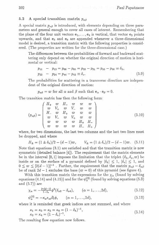
5.2 A special transition matrix Pcr{3

A spec ial matrix Pcr{3 is introduced , with elements depending on three para­meters and general enough to cover all cases of int erest . Remembering tha tthe plane of the four unit vect ors e1, . . . , e4 is vertical, that vect or e2 pointsupwards, and that e5 and e6 are appended whenever a three-dimensionalmodel is desired, a transition matrix with the following properties is consid­ered. (The properties ar e written for the three-dimensional case .)

The differences between th e prob ab ilities offorward and backward scat­te ring only depend on whether the original direction of motion is hori­zontal or vertical:

PnP22

P13 = P66 - P65 = P33 - P31 = P55 - P56 == Ok ,

P24 = P44 - P42 == OV' (5.9)

(5.10)

(5.14)

(5.12)

(5.13)

The probabilities for scattering in a tr ansverse directi on are indepen­dent of the orig inal direction of motion:

Pcr{3 = tv for all a and (:J such that e ., . e{3 = O.

The transit ion matrix has then th e following form :

H + tv H _ tv tv tvtv V+ tv V_ tv tv

()H _ tv H+ tv tv tv

Pcr{3 = V Vtv _ tv + tv tvtv tv tv tv H+ H_tv tv tv tv H _ H+

where, for two dimensions, the last two columns and the last two lines mustbe dropped, and where

H± = (1 ± ok)/2 - (d - l)tv , V± = (1 ± ov)/2 - (d - l)tv . (5.11)

Not e that equations (3.1) are sat isfied and th at the transition matrix is nowsymmetric (detailed balance [4]). The requirement that th e matri x elementsbe in the interval [0, 1] imposes the limitation that the triplet (Ok , 0v, tv ) beinside or on the surface of a pyramid defined by lOki :::; 1, lovl :::; 1, ando :::; tv :::; [2(d - 1)]-1 . Further, th e requirement th at the matrix P",{3 - ocr{3be of rank 2d - 1 excludes th e base (tv = 0) of this pyramid (see figure 4).

With this transition matrix the expressions for the Xcr (found by solvingequations (4.14) and (4.15)) and for the 1f;~2) (found by solving equat ions (5.3)and (5.7)) are

X'" = _ 2~~~v1) <p2 ( 0"'2 - Ocr4), (a = 1, . . . , 2d),

1f;~2 ) = - ",,,, e,,,;!Ji<p , (a = 1, . . . , 2d),

where it is reminded that greek indices are not summed, and where

"'1 = "'3 = "'5 = "'6 = (1 - Ok)-l,"'2 = "'4 = (1 - ov)-l .

The resulting flow equation now follows.

Cellular A utom aton Model for Fluid Flow in Porous Media

Figure 4: Allowed values of (Oh, Ov , tv) are inside and on the surface ofthe pyramid, except its base. The height of the pyramid is [2(d- 1)t l

.

393

(5.15)

5.3 The flow equation

The flow equat ion is found by using equ ations (5.12) and (5.13) , togetherwith

2d

L:: e",i e ",j = zs.;0 = 1

in equation (5.8). Keeping in mind that the unit vect ors along the coor­dinate axes Xl , X2, and X 3 are, respectively, el, e2, and es , and that thetwo-dimensional model is obtained by dropping coordin ate X3 and unit vec­tor es , one finds:

1 + 8h 2 1 + s; ( 4, 2)at<p - 4(1 _ 8h)al <P - 4(1 _ 8

v) a2 a2<P + 1 + 8

v<P = 0

in two dimensions, and

in three dimensions. For a direct comp arison of these equatio ns wit h thedimensionless equat ions of section 2, a scale <Po of order of magnitude 1 isintroduced for <P,

<P = <Po iP .

Equations (5.15) and (5.16) can now be written

a iP - etdl [a2+ (d - 2)a2JiP - C(dla (a iP +C(dl iP2) = 0t hI 3 v 2 2 9 ,

(5.17)

(5.18)

394

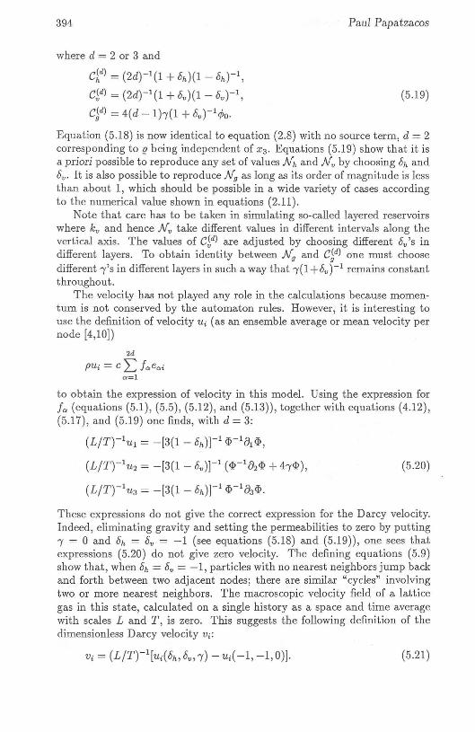
whe re d = 2 or 3 and

Paul Papatzacos

(5.19)

C~d) = (2d)- 1(1+ oh )(l - Oh)- l ,

C~d) = (2d)-1(1 + ov)(l - ov)-l ,

C~d) = 4(d - 1),(1 + ov)-l</JO'

Equation (5.18) is now identical to equation (2.8) with no source term, d = 2corresponding to (! being independent of X 3' Equations (5.19) show that it isa priori possible to reproduce any set of valu es Nh and s; by choosing Oh andov. It is also possible to reproduce Ny as long as its order of magnitude is lessthan ab out 1, which should be possible in a wide variety of cases accordingto the numerical value shown in equations (2.11) .

Note t hat care has to be taken in simulating so-called layered reser voirswhere k; and hence Nv take different values in different inte rvals along thevertical ax is. The valu es of C~d) ar e adjuste d by choosing different ov's indifferent layers . To obtain identity bet ween Ny and C~d) one must choosedifferent , 's in different layers in such a way that ,(1+ov)-l remains const antthroughout.

The velocity has not played any role in the calculations because momen­tum is not conserved by the automaton rules. However, it is interesti ng touse the definition of velocity Ui (as an ensemble aver age or mean velocity pernode [4,10])

2d

PUi = c L fc, eerier=l

to obtain the expression of velocity in this model. Using the expression forf er (equations (5.1), (5.5), (5.12) , and (5.13)) , together with equations (4.12),(5.17), and (5.19) one finds , with d = 3:

(L/T)- lU1 = - [3(1 - Oh )t1 <I> - lOl <I> ,

(L/T)-lU2 = -[3(1 - ov )t1 (<I> - 102<I> + 4,<I» , (5.20)

(L/T) - lU3 = -[3(1 - Oh)t1 <I>-103<I> .

These expressions do not give the corre ct expression for the Darcy velocity.Indeed , eliminat ing gravity and setting the permeabi lities to zero by putting, = 0 and Oh = S; = -1 (see equations (5.18) and (5.19)) , on e sees thatexpressions (5.20) do not give zero velocity. The defining equat ions (5.9)show that, when Oh = Ov = - 1, particles with no nearest neighbors jump backand forth between two adj acent nodes; there are simi lar "cycles" involv ingtwo or more nearest neighbors . The macroscopic velocity field of a latticegas in this state, calculat ed on a single history as a space and time averagewith scales Land T , is zero. This suggests the following definition of thedimensionless Darcy velocity v;:

(5.21)

Cellular Automaton Model for Fluid Flow in Porous Media

Using expressions (5.20) one then find s

_ C( 3)"'-I!::>'"VI - - h "" ul"" ,

V2 = _C~3) (<1> -182<1> + cy)<1»,

_ C(3) ", -I!::> '"V3 - - h "" u 3"" ·

395

(5.22)

Comparing equat ions (5.18) an d (5.22) with equations (2.8) and (2.10) onesees that Vi has the correct exp ression.

It may be objected to this deri vation that the Darcy velocity given byexpressions (2.10) vanishes with the horizontal and vertical permeabilities,even with a nonzero gravity term, so that the renormalizing te rm in equa­tion (5.21) should be Ui( -1, - I,,). However, equat ions (5.18) and (5.19)show that the gravity term for the lat ti ce gas is proport ional to "t / (1 +bv ) sothat it is neces sary to set, = 0 when bv = -1. Also, the argument can becarried out as a limiting procedure, where bh and bv are made to approach-1 , so as to avoid a confrontation with the fact that values bh = - 1 andS; = - 1 ar e not allowed (see figure 4) .

6 . F ir st numerical check: Two-dimensional flo w w ith out gr av it y

In this sect ion , the cellular automaton will be checked agai nst an analyticalcalculation . A model is set up in such a way that it is pos sible to solvethe diffusion equat ion analytically, which mean s that very simple boundariesand boundary conditions are chosen. T he boundary is a square, with thecondition that no flow takes place across it . A source, at the cente r of thesqu are , injects fluid at a (preferably) const ant rate, starti ng wit h no fluidat zero time. The simulation of such a situat ion with a cellular au tomatonpresents no problems as far as the no-flow boundar y is concerned. Particlecreation at a constant rat e is, however , not st raightforward because of therule that there is at mos t one particle per state.

The additional rule concern ing creati on , and t he resulting modificationof equation (5.15) , will be considered first. Let the source be located atnode r~ and let O",,(r',t') be the probability of creat ing an e,,-particle at r'and t' (O",,(r' ,t') =I 0 only if r' = r~) . Equations (4.1) and (5.18) become,respect ively,

f ,,(r' + ).e", t' +T) - f ,,(r', i') = n" + 0"",

and

where

4

0" = L 0"".,,=1

(6.1)

(6.2)

396 Paul Pspeizecoe

In equation (6.1), a 1- 0 only inside a squ are region wit h side e an d cent eredat r~ . The order of magnitude of a can be estimated by referring to theassumption that the fluid density is at most of order e (see equation (4.12)).The number of particles created afte r T IT time steps is about (T IT)a . Thefirst particles created have traveled a distance of the order of .j(T IT) so thatthe average particle density created is of the order of (T IT)aI (.j(T IT))2 = a.Since this must be 'at mos t of order e one may set

a = et/; (6.3)

(6.5)

so that the right-hand side of equa tion (6.1) is vl(4€2) where u, like 5, isdifferent from 0 only inside a square region with side e and centered at(Xl = Xl., X2 = X2s )' It follows that, when e -> 0, equation (6.1) can bewritten

ati]> - ci2)a;i]> - c~2)a;i]> = (v/4)8(Xl - xls)8(X2 - X2s ), (6.4)

where 8(x) is the Dirac delta function.As already mentioned, the lattice is assumed to be squa re. Let the length

of its side be N.\ where N is odd so t ha t there is a cent ral node whereparticle creation takes place. The automaton can be run when a choice hasbeen made for 8h , 8v , tv, and for a = ev . T he bound ari es of the square aresuch that all particles arriving there are reflected (wit h an initially emptylattice, there will never be any particles tangential to the boundary). T hecent ral node creates an e,, -parti cle with a probab ility euI4 if such a particledoes not already occupy the node. Particle densit ies are then calculate d andcompared with the ana lytical solution of equation (6.4) .

The properties of the analytical solution ar e now bri efly examined. It isconvenient for simplicity to introduce the following notation:

- ) C(2)C(2)p - v h'

The fact that one mus t work with a low density of part icles, toget her wit hthe rule that a particle is created at the central node only if a particle of thesame type does not already occupy the node , means tha t a constant rate ofcreation cannot be exactly maintained so that it is necessary t o consider atime-dependent v on the right -hand side of equa t ion (6.4). Wit h i]> = 0 atzero t ime one can then wri te the solution as

i]>(~, TJ , B) = ~ (o v (B')G(~, TJ, B- B' )s«,4p Jo

where the Green function G is given by [2J

(6.6)

00 00

G(~, TJ ,B) = 1 + 2 L e- 4>r

2n

20j r cos(n1rO +2 L e- 4

>r2n

20r cos(n1rTJ )

n =l n = l00 00

+ 4 L L e- 4>r

2(m

2j r+ n

2r )Ocos(m1rO cos(n1r TJ )· (6.7)

m=l n = l

In these equations, the space coordinates ~ and TJ have their origin at thecent ral node and vary between - 1 and + 1 (see figure 5). T he t ime var iab le B,

Cellular Automaton Model for Fluid Flow in Porous Media

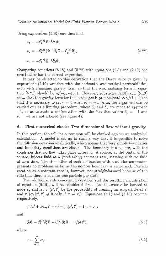
when related to the number of time st eps i'[r (see section 4), is

397

t'/T0= ­

No'(6.8)

which shows that the appropriate unit of time, in number of t ime steps, isNo·

Particle densities obtained during the automaton ru n must be comparedwith numerical values given by equat ion (6.6) . Actually, the calculation ofparticle densities involves an averaging of particle numb ers in both space andtime. In terms of the coordinates (~ , TJ , 0) introduced above, let £l{ be thelinear dimension of the space averaging region and £lo be the t ime averag inginterval. In lattice terms there will be N2£l~ sites in a space averaging regionand, according to equation (6.8), there will be N 2 £lo/ p ti me st eps in a timeaveraging interval. In the automaton runs described below there are twospace averaging regions, centered at (~ = 1/2, TJ = 0) (lab eled E in figur e 5)and at (~ = 0, TJ = 1/ 2) (labeled N in the same figur e).

Time averaging is done as follows. One first chooses a final time 0 = Of>a mu ltiple of the averaging int erval £lo. T his determines, through equa­t ion (6.8), the maximum number of time steps the automaton is to be run ,namely OfN 2 / p. (It will be shown below that the choice of Of can not be madearbitrarily.) Space averages are registered at each time ste p, over a numberof time steps corresponding to £lo, namely N 2£lo/ p, and the mean value andst andard deviation are calculated. This standard devi ation is assumed to bean est imate of the "experiment al err or" attached to the mean value . In prin­ciple both the mean value and the standard deviation sho uld be calculatedby repeating the experiment many t imes and recording the space average ata given time. The standard deviation calculat ed as described above is some-

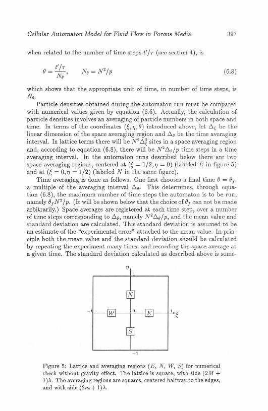
Figure 5: Lattice and averaging regions (E, N , W, S) for numericalcheck without gravity effect. The lattice is square, with side (2M +1». . The averaging regions are squares, centered halfway to the edges,and with side (2m +1)>..

398 Paul P apatzacos

what larger t han its corre ct value because the mean values vary with t imeinside the time averaging interval.

T he mean value itself could be assumed to be an estimate of particledensity at the center of the space averaging region and in the middle ofthe time averaging regio n, to be compared with th e numbers given by theanalytical expression, equa tion (6.6) . It is preferable, however, to comparethe above mean value with the analyti cal expression obtained by averagingequat ion (6 .6) over the corre sponding space and time regions . This allows tochoose values for ~e and ~B which are not too small.

It remains to define the v-function in equat ion (6.6) . The automatonrun s are started with a "requeste d" crea t ion probab ility (J = (Jreq (i.e., u =t/req according to equation (6.3)) . T he expected number of particles createdbetween t ime 8 and 8 + ~B is N 2~B(Jr eq / p . T he act ual number of particlescreated var ies, however , because of statistical fluctuations bu t also because ofthe ru le that a particle is created only if a particle of the same type does notalready exist at the cent ra l node. For examp le, in one of the runs presentedbelow, (Jreq = 0.05 and the int erval ~B corre sponds to 1020 time steps , sothat the expected nu mber of particles created per ~B-interval is 51. T heactua l numbe rs regi stered in successive ~B-intervals are, however ,

50,36,49,52,40,53,40,54, .. . .

To account for these variations , equatio n (6.6) is writ ten

<P(~, TJ, 8) = <Po foBV(8')G(~, TJ, 8 - 8') d8',

<Po = vreq/( 4p), v(8) = v(8)/vreq

where v(8) is defined by

v(8) = Vk for (k - l)~B ::::: 8 ::::: k~B ,

and

(6.9)

(6.10)

(6.11)

, Number of particles create d for (k -l)~B ::::: 8 ::::: k~B~ = .

N2 ~B!Jreq/P

Referring to the example already mentioned, the first numbers III the Vksequence are

50/51,36 /51,49/51,52/51,40/ 51,53/ 51,40/ 51, 54/51, . . . .

Returning now to the averaging of the an alytical expression over space andtime and referring to equatio n (6.9) , a fun cti on (<Ph is defined as the averageof <P/<Po in region E of figure 5 an d in the interval [(k - 1)~B , k~B ] :

1 l ktl e 1 jtleJ2(<P )k = - d8- dTJ~B (k-l)tl e ~~ - tl eJ2

1(I+ tl~ ) /2 foB

d~ v ( 8')G (~ , TJ, 8 - 8') d8' .( 1-tl~)/2 0

Cellular A utomaton Model for Fluid Flow in Porous Media 399

The calculation of this expression with the Green function given by equa­tion (6.7) is straightforward but tedious. The det ails are not given here.

Figure 5 shows four space averaging reg ions, labeled E, N, W, and 5,centered halfway from the lat t ice center to the edges , and with side equal tot.~. Because of symmet ry, the analytical particle density averaged, at a givent ime, in region E can be compared to the average number of particles, at thecorresponding t ime step , in region E +W (or in region E +W +N +5 if r = 1).If r =I- 1, t he average number of particles in region N +5 can, because of theform of the Green function, be compared to the above mentioned analyticalaver age provided l /r is substituted to r in equation (6.7).

Finally, the space-time averages of particle numbers obtained from run­ning the automaton must be normalized in a manner which is comparableto the normalization of (<I» k' i.e . by dividing them by <I>o . Recalling equa­t ion (4.12), one must also divide by 4c, so that the normalized and averagedparticle number is

(p )f

Po

(Space-t ime average of particle numbers)/Po,

O'req / p,

(6.12)

where k refers to the interval [(k - l )t.o, kt.o], and R is either E + W orN +5 (when r = 1, R is E +W +N +5). Note that neither (<I>h nor (P)kdirectly depend on c. This parameter is, however, indirectly present throughO'req which must be at most of order c.

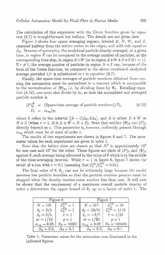
The results of two experiments are shown in figures 6 and 7. The para­met er values for each experiment are given in table 1.

Note that the lat tice sizes are chosen so that N 2 is approximately 104

for one case and 105 for the other. These figure s are plots of (P)k and (<I> hagainst {} , each average being allocated to the value of {} which is in the middleof the t ime-averagi ng interval. While r = 1 in figure 6, figure 7 shows theresult of a run with r = 0.1 (mean ing that C~2)/d2

) = 0.01).

The final value of {}, {}f> can not be arbitrarily large because the modelassumes low particle dens ities so that the particle creation process must besto pped when the density reaches some number less than one. It will nowbe shown that the requirement of a maximum overall particle density oforder c determines the upper bound of (}f up to a factor of order 1. The

Figure 6 Figure 7N = 101 C~2) = 1 N = 317 C~2) = 10

Oh = 3/5 C~2) = 1 s, = 39/41 C~2) = 1/10Ov = 3/5 r = 1 Ov = - 3/ 7 r = 1/10

tv = 1/10 p =l tv = 1/82 p =lO'req = 0.05 No = 10201 O'r eq = 0.05 No = 100489

t.~ = 0.2, t.e = 0.1 t. ~ = 0.2, t.e = 0.1

Table 1: Parameter values for the automaton runs illustrated in theindicated figures.

400 Paul Papatzacos

2.0

1. 0

1.0 2.0

Figure 6: Plot of the space and time averaged particle-numbers givenby equat ion (6.12) ((- ) with "error bars " extending one standard de­viation above and one below) , and of the corresponding analyticalaverages given by equation (6.11) (0) versus time fl. Th e parametervalues are given in table 1. In particular, r = 1.

2.0

1.0

1.0 2.0

Figure 7: Plot of the space and time average d particle-numbers givenby equation (6.12) ((-) for the E + W averages and (x ) for the N +S averages, with "error bars" extending one standard deviation aboveand one below) , and of th e corresponding analytical averages givenby equation (6.11) ((0) and (0)) versus time fl. The parameter valuesare given in table 1. In particular, r = 0.1.

number of time steps necess ary to reach 8J being N 28J/ p, the approxim atetotal number of particles created is N 28

jO"req /P , so that the maximum overalldensity is 8jO"req/P. W ith O"req = cVr eq on e sees t hat

where t he proportionality factor is of order 1. T hus , for given P, the wayto explore large t imes is to reduce the particle creation probabi lity. In bothautomaton "exp eriments" presented above one has in mind a value of e equalt o 0.1 and the value of 8J corresponds to a m aximum overall particle den sityeq ual to 0.1.

Cellular Automaton Model for Fluid Flow in Porous Media 401

All other parameters being constant, the standard deviati ons are roughlypr oporti onal to N - 1

/2

. It should also be noted that, a value of 8f being given ,calculation time on a sequential computer is proportional to N 4 (N5

) for ato-dimensional (three-dimensional) simulation. A power of 2 (3) accounts forthe number of nod es and an additional power of 2 accounts for the numberof time steps.

Equ ations (5.18) and (5.19) show th at the probability for right anglescattering, tv, is not "measura ble," i.e., it does not appear in th e numericalcoefficients. The particular choice of tv in any automat on run is thus onlylimited by the fact that the point of coordinates (Ok,ov, tv) must be inside th epyramid of figure 4. In the automaton runs referred to in this and the nextsection, tv has been arbitrarily chosen halfway up from the point (Ok ,Ov,O)on the pyramid base, to the point (Ok, ov, tvmax) on the pyramid side.

It shou ld finally be noted that the flow equations without the gravityterm are linear. The quantity denoted above by (P) , given by a cellularautomaton run , is then a numerical solut ion of equation (6.1) where <P isreplaced by <P - <Pi (with <Pi an arbitrary constant, for example an initi alvalue of <p). It is also a numerical solution of the same equation with <Preplaced by <Pi - <P and 0" replaced by - 0" , meaning that one has a practicalway of simulating dep letion by an automa ton run with particle crea t ion anda subsequent change of sign in the int erpretation of the results.

7. Second numeri cal check: One-dimensional flow with gravity

As in the previous section, an automaton run is checked against an analyticalsolution of equation (5.18) , where d = 2 and <P is assumed independent ofX l> so that it becomes

(7.1)

(7.5)

This equat ion is nonlinear and no analytical solut ion is known . It is howeverpossible to chose the start and boundary condit ions in such a way tha t thesolut ion evolves to a time independent function , <P 00 (X2)' One can th encompare the long time prediction of the automaton with <P 00 (X2)' A possibleset of such start and boundary conditions is the following :

<P = 1 at X2 = 0, (7.2)

<P=O at X2 = Ne, (7.3)

<P=O at t = O. (7.4)

It is reminded that the automaton lat t ice is square, with side N A, whichexplains the right-hand side of equat ion (7.3) . Function <p oo is the solutionto equations (7.1) (without th e Or term) , (7.2), and (7.3). The differentialequation is of the Riccati type and one finds [5J

<p oo = tan[a(l - OJ ,tan a

402

where

and a is the solution of the t ra nscendental equat ion

Paul Papatzacos

(7.6)

(7.7)atana = C~2)N£ = 4£<po INc .1 + u"

On the right -hand side of this last equation, <Po is a scale for ep (see equa­tion (5.17)) . Since ep is set equal to 1 at the lower boundary by equation (7.2),the product 4£<po is, in lattice terms , the particle density at the lower bound­ary. Thus the automaton is run with reflecting right and left boundaries,a lower boundary with a constant particle densi ty and an upper boundarywith zero particle density. The condition at the upper boundary is easi lyimplemented by annihilating all particles ar riving there . The condition atth e lower boundary is managed as follows. At the end of each time ste p, afte rthe rul es for particle movement have been applied , all particles are removedfrom the lower boundary and then, at preselected site s (say at each tenthsite from the left , for a lat tice with 100 sites on a side) particles of randomtypes are created.

To compare the automaton output with equation (7.5) it is necessar y t oknow the t ime scale of the solution of equation (7.1). An est imate of thistime scale can be obtained by linearizing the equation, i.e., setting C~2) = o.The solution of the linear equation, with start and boundary conditions givenby equations (7.2-7.4), is [2]

where ~ is defined by equation (7.6) and (compare with equation (6.8))

t']«B= No ' (7.8)

eplin is very nearly time-independent as soon as Breaches the value 1 becauseof the exponent ial factors in the sum. It is therefore assumed that the au­tomaton stabilizes, except for statistical fluctuations, for all time steps largerthan 2No.

A square lattice with N = 100 sites on a side has been chosen, toget herwith constant particle density at th e lower boundary 4£<po = 0.1, and C~2) =1. This implies No = 104

. Apart from that, two cases are pres ented withdifferent scattering probabilities, as shown in table 2. Particle averages arecalcu lat ed in space with .0.e = 0.1 and normalized through division by theparticle density at the lower boundary (4£<po) . Each space average is recordedfor all time steps, starting at time step number 2 x 104 (B = 2) and endingat time step number 4 x 104 (B = 4). Mean values and st andard deviationsare calculated and the mean values are compared to th e values given by

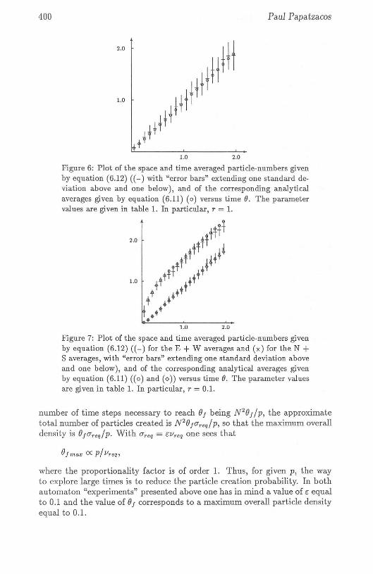
Cellular Automaton Model for Fluid Flow in Porous Media

Figure 8 Figure 9Ok = 3/5 Ok = 0s; = 3/5 Ov = 3/5

tv = 1/10 tv = 1/10,=1 ,= 1/2

Table 2: Parameter values for the automaton runs illustrated in th eindicated figures.

403

equat ion (7.5). Actually, since the space averag ing region D.{ is ap prec iablylarge , the comparison is done with

(<1» ( = _1 (AI <1>00(0 d~ = 1 In cos[a(l - £D.{)] (7 9)D.{ J«(-l)A I D.{a t an a cos[a(l - (£ - 1)D.{ ]· .

The space averaging intervals are numbered from the bottom (£ = 1) to thetop (£ = 1/D.{) of the lat t ice.

The results are shown in figures 8 and 9, wh ere each space averagedvalue is allo cated to the ~- coordinate in the middle of the int erval. T here isagreement to within one standard deviation for most po ints .

8 . Conclusions

A cellular automaton model for the simulation of one-phase liquid flow inporous media has been derived , and a set of simple checks has b een pr esented.The simulations were don e with FORTRAN programs on a MicroVax 3500.It took somewhat more than a CPU-hour to produce the dat a for figur e 6 andabout five days to produce the data for figur e 7. More effect ive simulations

1.0

0 .5

t ++

0 .5 1.0

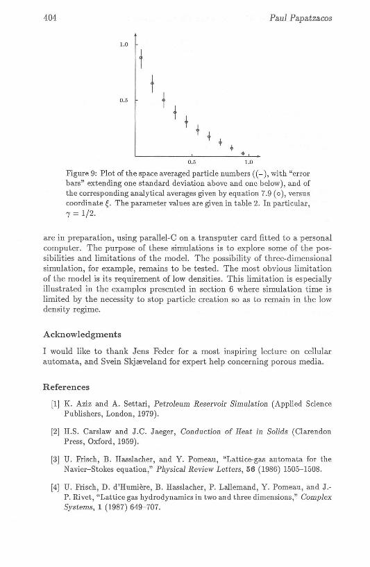
Figure 8: Plot of the space averaged particle numb ers ((- ), with "errorbar s" exten ding one standard deviation above and one below), and ofthe corresponding analytical averages given by equation 7.9 (0) , versuscoordinate t . The parameter values are given in table 2. In particular ,, =1.

404 Paul Papatzaco s

1.0

t0.5

0 .5 1.0

Figure 9: Plot of the space averaged particle numb ers ((- ), with "errorbars " ext ending one standard deviation above and one below), and ofth e corresponding analytical averages given by equation 7.9 (0), versuscoordinate ~. Th e parameter values are given in table 2. In particular ,'Y = 1/2.

are in preparation, using parallel-C on a transputer card fitted to a personalcomputer . The pur pose of these simulations is to explore some of the po s­sibilit ies and limitations of the model. The possibility of three-dimen sion alsimulation, for example, remains to be tested . The most obvious limitationof the mo del is its requirement of low densities. T his limit at ion is especiallyillust rat ed in the examples presented in section 6 where simulation t ime islimi ted by the necessity to stop particle creation so as to remain in t he lowden sity regime.

A ckn owledgment s

I wou ld like to thank J ens Feder for a most inspiring lect ur e on cellularautomata, and Svein Skjeeveland for expert help concerning porous media.

Refe ren ces

[1] K. Aziz and A. Settari, Petroleum Reservoir Simu lation (Applied SciencePublishers, London, 1979).

[2] H.S. Carsl aw and J .C. Jaeger, Conduction of Heat in Solids (ClarendonPress , Oxford, 1959).

[3] U. Frisch, B. Hasslacher, and Y. Pomeau, "Lattice-gas automata for theNavier- Stokes equation," Physical Review Letters, 56 (1986) 1505-1 508.

[4] U. Frisch, D. d'Humiere, B. Hasslacher, P. Lallemand, Y. Pomeau, and J .­P. Rivet , "Lat tice gas hydrodynamics in two and three dimensions, " ComplexSystems, 1 (1987) 649-707.

Cellular Automaton Model for Fluid Flow in Porous Media 405

[5] E.L. lnce, Ordinary Differential Equations (Dover , New York, 1956).

[6] L.D. Landau and E.M . Lifshitz, Fluid Mechanics (Pergamon Press, Oxford ,1959).

[7] D.H. Rothman, "Cellular-automaton fluids: A model for flow in porous me­dia," Geophysics, 53 (1988) 509-518 .

[8] W .G. Vincenti and C.H. Kruger, Jr., Introduction to Physical Gas Dynamics(Robert E. Krieger Publishing Company, Malabar , Florida, 1965).

[9] S. Whitaker, "Flow in porous media l: A theoretical derivation of Darcy'slaw," Transport in Porous Media, 1 (1986) 3-25.

[10] S. Wolfram, "Cellular automaton fluids 1: Basic theory," Journal of Statis­tical Physics, 45 (1986) 476-526.