Cellular Automata

This is week 7 of Biologically Inspired ComputingVarious credits for these slides, which have in part been adapted from slides by: Ajit Narayanan, Rod Hunt, Marek Kopicki.

Cellular Automata

A CA is a spatial lattice of N cells, each of which is one of k states at time t.•Each cell follows the same simple rule for updating its state.

•The cell's state s at time t+1 depends on its own state and the states of some number of neighbouring cells at t.

• For one-dimensional CAs, the neighbourhood of a cell consists of the cell itself and r neighbours on either side. Hence, k and r are the parameters of the CA.

•CAs are often described as discrete dynamical systems with the capability to model various kinds of natural discrete or continuous dynamical systems

SIMPLE EXAMPLESuppose we are interested in understanding how a forest fire spreads. We can do this with a CA as follows.

Start by defining a 2D grid of `cells’, e.g.:

This will be a spatial representation of our forest.

SIMPLE EXAMPLE continuedNow we define a suitable set of states. In this case, it makes sense for a cell to be either empty, ok_tree, or fire_tree – meaning: empty: no tree here ok_tree: there is a tree here, and it’s healthy fire_tree: there is a tree here, and it’s on fire.

When we visualise the CA, we will use colours to representthe states. In these cases; white, green and red seem the rightChoices.

SIMPLE EXAMPLE continuedNext we define the neighbourhood structure – when we run our CA, cells will change their state under the influence of their neighbours, so we have to define what counts as a “neighbour”. You’ll see example neighbourhoods in a later slide, but usually you just use a cell’s 9 immediately surrounding neighbours. Let’s do that in this case.

Next we decide what the neighbourhood will be like at the boundaries of the grid.

Example of 1-D cellular automaton

•For a binary input N long, are there more 1s than 0s?

•Set k=2 and r=1 with the following rule:

000 001 010 011 100 101 110 111

0 0 0 1 0 1 1 1

Cell + 2 neighbours:

Result:

That is, the value of a cell at time t+1 will depend on its value and the values of its two immediate neighbours at time t.

This is a form of ‘majority voting’ between all three cells.

Density classification

•In the above example, we have assumed wrap-around, and r=1.

•In this case, the CA has reached a ‘limit point’ from which no escape is possible.

•CAs have been used for simulating fluid dynamics, chemical oscillations, crystal growth, galaxy formation, stellar accretion disks, fractal patterns on mollusc shells, parallel formal language recognition, plant growth, traffic flow, urban segregation, image processing tasks, etc …

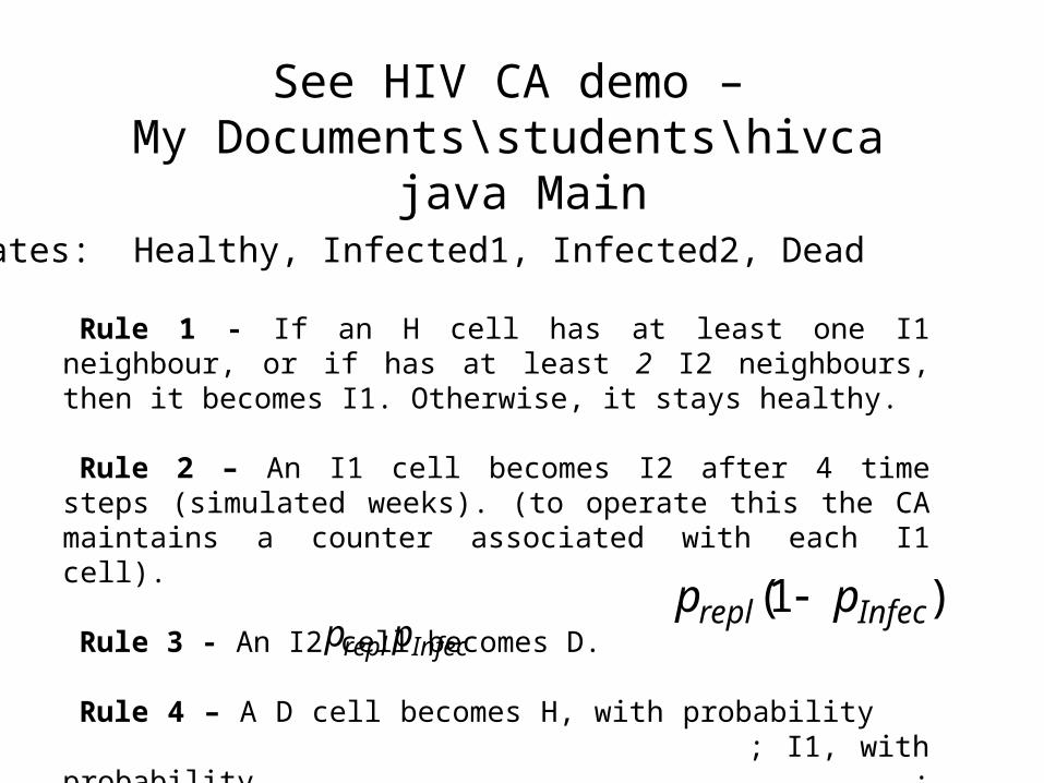
See HIV CA demo – My Documents\students\hivca java Main

Rule 1 - If an H cell has at least one I1 neighbour, or if has at least 2 I2 neighbours, then it becomes I1. Otherwise, it stays healthy.

 Rule 2 – An I1 cell becomes I2 after 4 time steps (simulated weeks). (to

operate this the CA maintains a counter associated with each I1 cell). Rule 3 - An I2 cell becomes D. Rule 4 – A D cell becomes H, with probability ;

I1, with probability ; otherwise, it remains D

)1( Infecrepl pp Infecrepl pp

4 states: Healthy, Infected1, Infected2, Dead

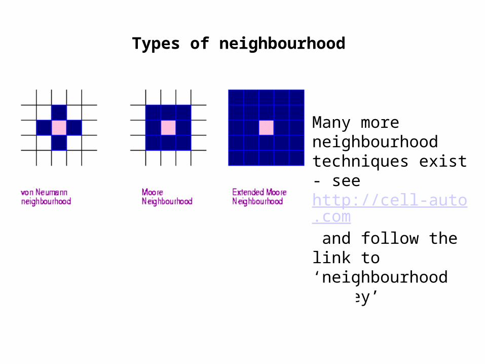
Types of neighbourhood

Many more neighbourhood techniques exist - see http://cell-auto.com and follow the link to ‘neighbourhood survey’

Classes of cellular automata (Wolfram)Class 1: after a finite number of time steps, the CA tends to achieve a unique state from nearly all possible starting conditions (limit points)

Class 2: the CA creates patterns that repeat periodically or are stable (limit cycles) – probably equivalent to a regular grammar/finite state automaton

Class 3: from nearly all starting conditions, the CA leads to aperiodic-chaotic patterns, where the statistical properties of these patterns are almost identical (after a sufficient period of time) to the starting patterns (self-similar fractal curves) – computes ‘irregular problems’

Class 4: after a finite number of steps, the CA usually dies, but there are a few stable (periodic) patterns possible (e.g. Game of Life) - Class 4 CA are believed to be capable of universal computation

John Conway’s Game of Life

• 2D cellular automata system.

• Each cell has 8 neighbors - 4 adjacent orthogonally, 4 adjacent diagonally. This is called the Moore Neighborhood.

Simple rules, executed at each time step:

– A live cell with 2 or 3 live neighbors survives to the next round.

– A live cell with 4 or more neighbors dies of overpopulation.

– A live cell with 1 or 0 neighbors dies of isolation.

– An empty cell with exactly 3 neighbors becomes a live cell in the next round.

Is it alive?

• http://www.bitstorm.org/gameoflife/

• Compare it to the definitions…

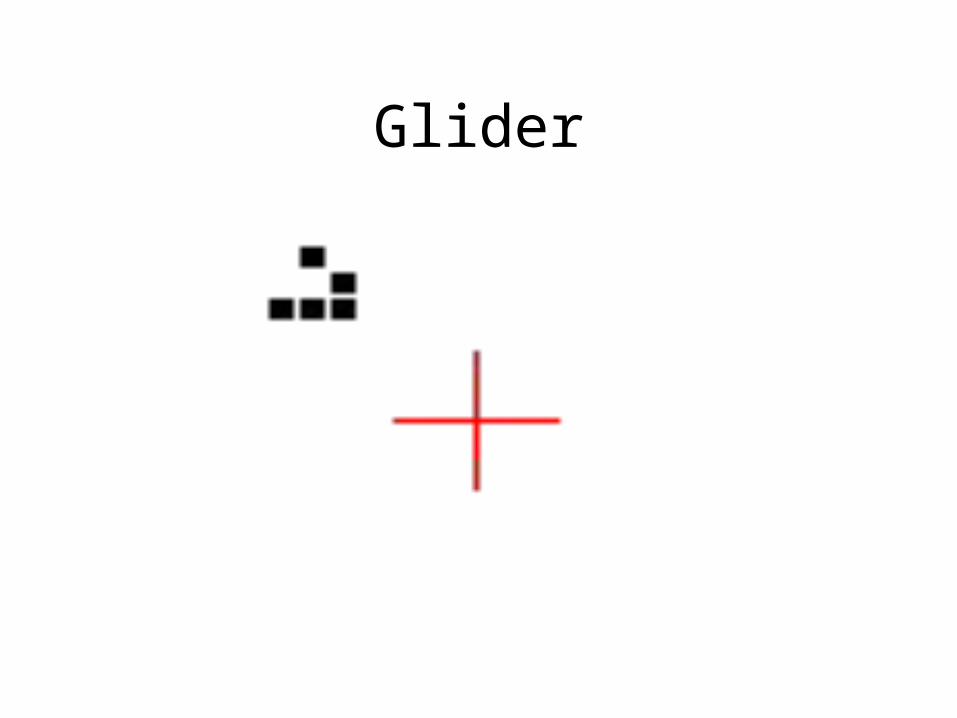
Glider

Sequences

More

Sequence leading to Blinkers

Clock

Barber’s pole

A Glider Gun

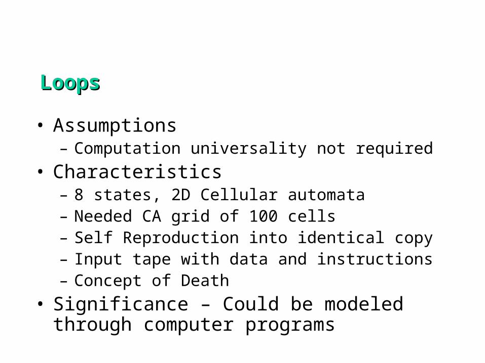
• Assumptions – Computation universality not required

• Characteristics – 8 states, 2D Cellular automata– Needed CA grid of 100 cells – Self Reproduction into identical copy– Input tape with data and instructions– Concept of Death

• Significance – Could be modeled through computer programs

LoopsLoops

Langton’s LoopLangton’s Loop

0 – Background cell state 3, 5, 6 – Phases of reproduction

1 – Core cell state 4 – Turning arm left by 90 degrees

2 – Sheath cell state state

7 – Arm extending forward cell state

Loop ReproductionLoop Reproduction

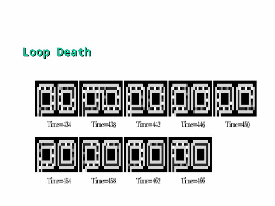
Loop DeathLoop Death

Langton’s Loops

Chris Langton formulated a much simpler form of self-rep structure - Langton's loops - with only a few different states, and only small starting structures.

There remains debate and interest about the `essentials of life’ issue with CAs, but their main BIC value is as modelling techniques.

Modelling Sharks and Fish:

Predator/Prey Relationships

Bill Madden, Nancy Ricca and Jonathan Rizzo

Graduate Students, Computer Science Department

Research Project using Department’s 20-CPU Cluster

We’ve seen HIV – here are some more examples.

• This project modeled a predator/prey relationship• Begins with a randomly distributed population of

fish, sharks, and empty cells in a 1000x2000 cell grid (2 million cells)

• Initially,– 50% of the cells are occupied by fish

– 25% are occupied by sharks

– 25% are empty

Here’s the number 2 million• Fish: red; sharks: yellow; empty: black

Rules

A dozen or so rules describe life in each cell:• birth, longevity and death of a fish or shark• breeding of fish and sharks• over- and under-population• fish/shark interaction• Important: what happens in each cell is

determined only by rules that apply locally, yet which often yield long-term large-scale patterns.

Do a LOT of computation!

• Apply a dozen rules to each cell

• Do this for 2 million cells in the grid

• Do this for 20,000 generations

• Well over a trillion calculations per run!

• Do this as quickly as you can

Rules in detail: Initial Conditions

Initially cells contain fish, sharks or are empty• Empty cells = 0 (black pixel)

• Fish = 1 (red pixel)

• Sharks = –1 (yellow pixel)

Rules in detail: Breeding Rule

Breeding rule: if the current cell is empty• If there are >= 4 neighbors of one species, and >=

3 of them are of breeding age,» Fish breeding age >= 2,

» Shark breeding age >=3,

and there are <4 of the other species:

then create a species of that type » +1= baby fish (age = 1 at birth)

» -1 = baby shark (age = |-1| at birth)

Breeding Rule: Before

EMPTY

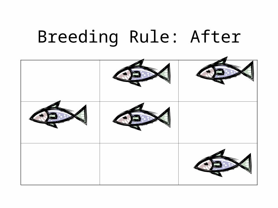
Breeding Rule: After

Rules in Detail: Fish Rules

If the current cell contains a fish:

• Fish live for 10 generations

• If >=5 neighbors are sharks, fish dies (shark food)

• If all 8 neighbors are fish, fish dies (overpopulation)

• If a fish does not die, increment age

Rules in Detail: Shark Rules

If the current cell contains a shark:

• Sharks live for 20 generations

• If >=6 neighbors are sharks and fish neighbors =0, the shark dies (starvation)

• A shark has a 1/32 (.031) chance of dying due to random causes

• If a shark does not die, increment age

Shark Random Death: BeforeI Sure Hope that the

random number chosen is >.031

Shark Random Death: After

YES IT IS!!! I LIVE

Spring 2005 JR 36

Sample Code (C++): Breeding

Results

• Next several screens show behavior over a span of 10,000+ generations

Spring 2005 BM 38

Generation: 0

Spring 2005 BM 39

Generation: 100

Generation: 500

Generation: 1,000

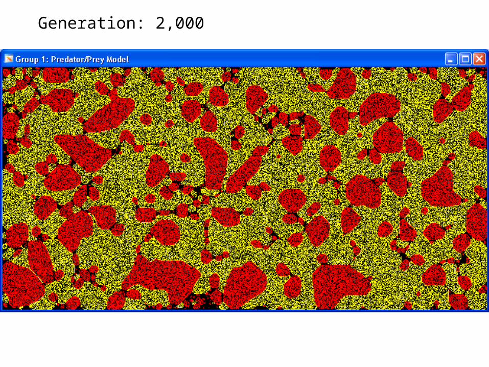
Generation: 2,000

Generation: 4,000

Generation: 8,000

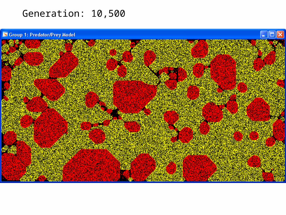
Generation: 10,500

Long-term trends

• Borders tended to ‘harden’ along vertical, horizontal and diagonal lines

• Borders of empty cells form between like species

• Clumps of fish tend to coalesce and form convex shapes or ‘communities’

Variations of Initial Conditions

• Still using randomly distributed populations:– Medium-sized population. Fish/sharks occupy:

1/16th of total gridFish: 62,703; Sharks: 31,301

– Very small population. Fish/sharks occupy:1/800th of total gridInitial population:

Fish: 1,298; Sharks: 609

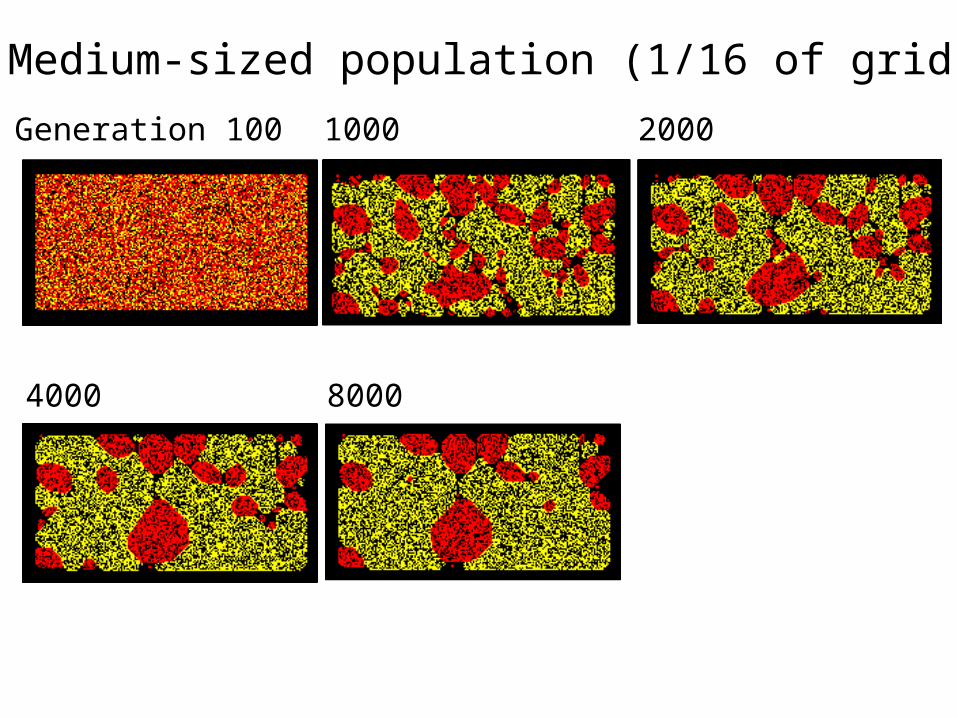
Generation 100 20001000

4000 8000

Medium-sized population (1/16 of grid)

Very Small Populations

• Random placement of very small populations can favor one species over another

• Fish favored: sharks die out

• Sharks favored: sharks predominate, but fish survive in stable small numbers

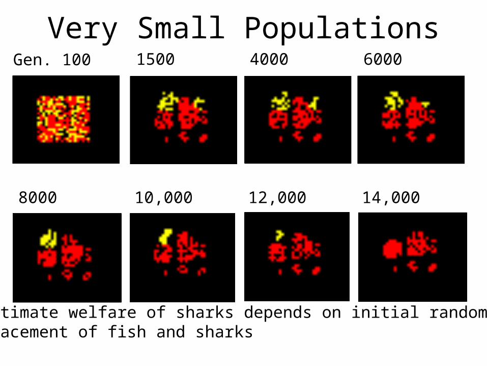
Gen. 100 4000 6000

8000

1500

10,000 12,000 14,000

Ultimate welfare of sharks depends on initial randomplacement of fish and sharks

Very Small Populations

Very small populations

• Fish can live in stable isolated communities as small as 20-30

• A community of less than 200 sharks tends not to be viable

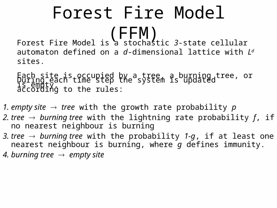
Forest Fire Model (FFM)

During each time step the system is updated according to the rules:

Forest Fire Model is a stochastic 3-state cellular automaton defined on a d-dimensional lattice with Ld sites.

Each site is occupied by a tree, a burning tree, or is empty.

1. empty site tree with the growth rate probability p 2. tree burning tree with the lightning rate probability f, if no nearest

neighbour is burning 3. tree burning tree with the probability 1-g, if at least one nearest neighbour

is burning, where g defines immunity. 4. burning tree empty site

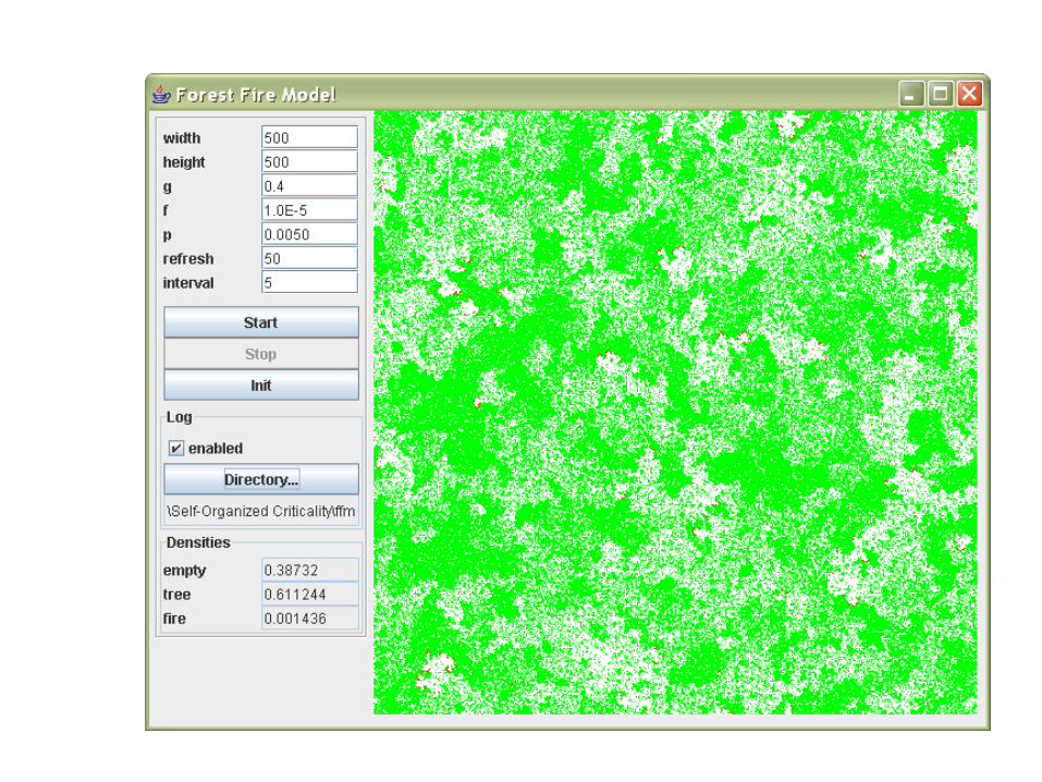
The application

Simulationforest density 45%

fire is not visible

The average cluster size is small in comparison to lattice size L.

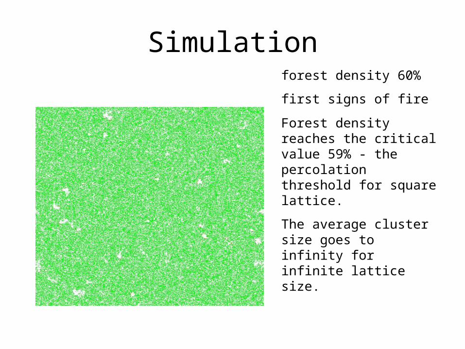
Simulationforest density 60%

first signs of fire

Forest density reaches the critical value 59% - the percolation threshold for square lattice.

The average cluster size goes to infinity for infinite lattice size.

SimulationFire spreads quickly burning down all connected tree clusters.

A variety of global structures emerges.

The whole process repeats and after some time forest reaches the steady state in which the mean number of growing trees equals the mean number of burning trees.

Next time

A bit more CAs, and L systems