Cellular AutomataJarkko KariSpring 2013

University of Turku

1 Preliminaries

1.1 Introduction

A cellular automaton is a discrete dynamical system that consists of a regular networkof finite state automata (cells) that change their states depending on the states of theirneighbors, according to a local update rule. All cells change their state simultaneously,using the same update rule. The process is repeated at discrete time steps. It turns out thatamazingly simple update rules may produce extremely complex dynamics when applied inthis fashion. A well known example is the Game-of-life by John Conway. Cellular automataare

• discrete in both space and time,

• homogeneous in space and time (same update rule at all cells at all times),

• local in their interactions.

Many processes in nature are governed by local and homogeneous underlying rules, whichmakes them amenable to modeling and simulation using cellular automata. For example,fluid dynamics can be modeled by moving point particles in a regular lattice, and the localupdate rule is designed to simulate particle collisions. Some of the most extensively inves-tigated concepts in cellular automata theory such as reversibility and conservation laws aremotivated by physics.

Cellular automata are also mathematical models for massively parallel computation. Sim-ple update rules can make the cellular automaton computationally universal, that is, capableof performing arbitrary computation tasks. Above mentioned Game-of-life is a good exam-ple. This point of view raises interesting questions concerning the computational aspects ofcellular automata.

A combination of the two viewpoints above (computational universality and modelingnatural processes) have made cellular automata a useful theoretical tool in the study ofcomputation in nature and the physical aspects and physical limits of computation.

These notes cover the basic theory of cellular automata. The most extensively used math-ematical tool is topology. It namely turns out to be a very natural and fruitful approach toconsider cellular automata as continuous functions on a compact metric space. This makescellular automata theory part of the field of topological dynamics, or more specifically, sym-bolic dynamics. Since only elementary topology is needed, no prior mathematics courses intopology are required: the notes contain a review of all the topology and symbolic dynamicsthat is needed.

Another tool that we use is the theory of computation and computability. We are ofteninterested in algorithmic questions related to cellular automata, and in many cases thesequestions turn out to be undecidable. A short review of computation theory, includinguniversality and (un)decidability is included to help students who have no familiarity withthis topic.

1

We start the notes with basic definitions and several examples of interesting cellular au-tomata. We then continue with classical results related to injectivity and surjectivity. Chap-ters that follow (not necessarily in this order) discuss linear (additive) cellular automata,reversibility, limit sets, classifications of cellular automata, universality, conservation laws incellular automata, topological dynamics of cellular automata, algorithmic questions, etc.

1.2 First example: Game-of-life

We start with a well-known example, Game-of-life, invented by John Conway in 1970. It isa cellular automaton that consists of an infinite grid of square cells — like an infinite graphpaper — where each square is colored white or black. The color is called the state of thecell. We say that a black cell is alive while a white cell is not. A coloring of the entire gridis called a configuration of Game-of-life.

There is a simple local update rule according to which the cells change their states. Thenew state of a cell only depends on the current states of the cell itself and its eight nearestneighbors:

• A living cell stays alive if and only if there are exactly two or three living cells amongthe eight surrounding cells. Fewer than two living neighbors causes death by isolation,more than three living neighbors by overcrowding.

• A non-living cell becomes alive if it has precisely three living neighbors — each organismhas three parents!

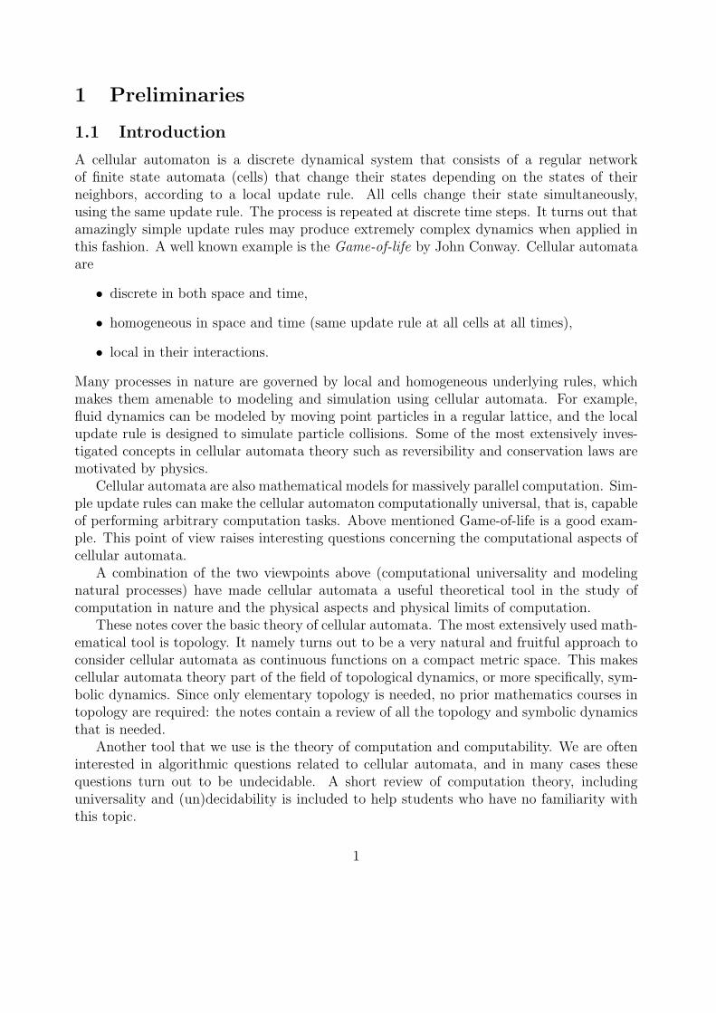
All cells use the same update rule, and all cells change their states simultaneously. Thischanges the coloring of the grid, i.e. the configuration changes into a new one. The processis then repeated over and over again, which creates a time evolution of the system. Figure 1shows an example of five consecutive generations of cells.

- - - -

Figure 1: Five steps of a time evolution in Conway’s Game-of-life.

Game-of-life is remarkable because the local update rule is extremely simple, but the long-time behavior of configurations is unpredictable. In the following the term ”finite pattern”refers to a configuration in which the number of living cells is finite. Conway showed that itis undecidable if a given finite pattern eventually dies completely out. In other words, thereis no (and never will be any as its existence is a logical contradiction) a computer program

2

that takes as input a finite pattern and always correctly determines if the input patterneventually dies out.

Over the years Game-of-life enthusiasts have compiled a vast library of patterns withvarious behaviors. The following terminology is used for various categories of objects:

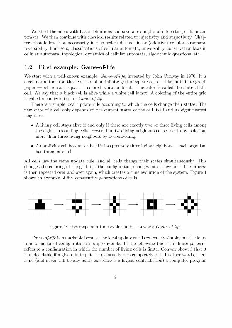
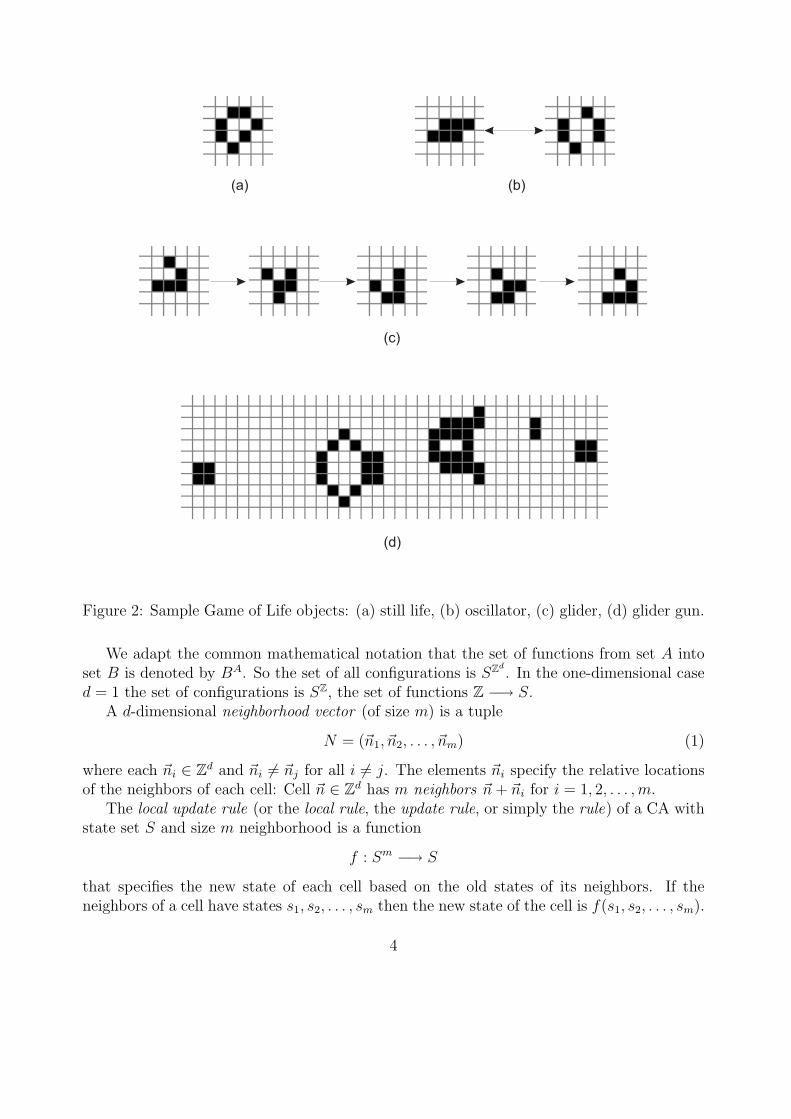
• still life: a fixed point pattern. The update rule keeps each cell unchanged. Thesimplest non-empty still life is the block, a two-by-two block of living cells. Anotherstill life is shown in Figure 2(a).

• oscillator : temporally periodic pattern. The update rule may change the pattern butafter some number of steps the original pattern reappears in the same location andorientation. Still life is a special type of oscillator. The smallest oscillator is the blinkerconsisting of three living cells in a line. Another oscillator with period two is shown inFigure 2(b).

• spaceship: a pattern that after some number of steps reappears, possibly in a differentlocation of the grid. A particular spaceship called glider is shown in Figure 2(c). Anoscillator is a stationary spaceship that does not move.

• gun: a finite pattern that — like an oscillator — periodically returns back to theinitial state, but in addition, emits spaceships. A glider gun emitting gliders is shownin Figure 2(d).

Objects from different categories emerge when Game-of-life is started in a random initialconfiguration. During the evolution the objects interact with each other through collisionswith gliders and other moving structures. Collisions create new objects which in turn par-ticipate in interactions, leading to extraordinary complexity.

1.3 Basic Definitions

This chapter introduces the most basic definitions and notations. Throughout these notes,abbreviation CA refers to cellular automata (plural) or cellular automaton (singular).

Let d be a positive integer. A d-dimensional cellular space is Zd. Elements of Zd arecalled cells. Let S be a finite state set. Elements of S are called states. A configuration of ad-dimensional CA with state set S is a function

c : Zd −→ S

that assigns a state to each cell. The state of cell ~n ∈ Zd is c(~n). A configuration should beunderstood as an instantaneous description, or a snapshot, of all the states in the system ofcells at some moment of time. Most frequently we consider one- and two-dimensional spaces,in which cases the cells form a line indexed by Z or an infinite checker board indexed by Z2,respectively.

3

(a) (b)

(c)

(d)

Figure 2: Sample Game of Life objects: (a) still life, (b) oscillator, (c) glider, (d) glider gun.

We adapt the common mathematical notation that the set of functions from set A intoset B is denoted by BA. So the set of all configurations is SZ

d. In the one-dimensional case

d = 1 the set of configurations is SZ, the set of functions Z −→ S.A d-dimensional neighborhood vector (of size m) is a tuple

N = (~n1, ~n2, . . . , ~nm) (1)

where each ~ni ∈ Zd and ~ni 6= ~nj for all i 6= j. The elements ~ni specify the relative locationsof the neighbors of each cell: Cell ~n ∈ Zd has m neighbors ~n + ~ni for i = 1, 2, . . . , m.

The local update rule (or the local rule, the update rule, or simply the rule) of a CA withstate set S and size m neighborhood is a function

f : Sm −→ S

that specifies the new state of each cell based on the old states of its neighbors. If theneighbors of a cell have states s1, s2, . . . , sm then the new state of the cell is f(s1, s2, . . . , sm).

4

In cellular automata all cells use the same rule, and the rule is applied at all cells simulta-neously. This causes a global change in the configuration: Configuration c is changed intoconfiguration c′ where for all ~n ∈ Zd

c′(~n) = f [c(~n + ~n1), c(~n + ~n2), . . . , c(~n + ~nm)]. (2)

The transformation c 7→ c′ is the global transition function of the CA. It is a function

G : SZd −→ SZ

d

.

Function G is our main object of study. Typically, function G is iterated, i.e. appliedrepeatedly, which produces a time evolution

c 7→ G(c) 7→ G2(c) 7→ G3(c) 7→ . . .

of the system. Here c is the initial configuration of the evolution, and the sequence

orb(c) = c, G(c), G2(c), G3(c), . . .

is the orbit of c. Time refers to the number of applications of G performed: Each applicationof G takes one time step, so Gt(c) is the configuration at time t, for all t = 0, 1, 2, . . ..

Sometimes we also consider two-way infinite orbits, i.e. sequences

. . . , c−2, c−1, c0, c1, c2, . . .

of configurations where G(ci) = ci+1 for all i ∈ Z. Here time t flows through all integers andthere is no initial configuration.

In summary: To specify a CA one needs to specify the following items (some of which maybe clear from the context):

• the dimension d ∈ Z+,

• the finite state set S,

• the neighborhood vector N = (~n1, ~n2, . . . , ~nm), and

• the local update rule f : Sm −→ S.

We therefore formally define the corresponding CA to be the 4-tuple A = (d, S, N, f). Theglobal transition function determined by these items according to (2) will be denoted byG[A], or simply by G when the CA A is clear from the context. Any function G that is thetransition function of some CA is called a CA function.

We usually identify a CA function G with the CA that determines it in the sense thatwe talk about cellular automaton G. Strictly speaking, however, the same function G isdetermined by different cellular automata (4-tuples). We say that two CA A and B areequivalent if G[A] = G[B]. Clearly equivalent CA have the same dimension d and state

5

set S but they may differ in their neighborhood vectors. However, we see in the followingsection that there is a unique equivalent CA whose neighborhood vector is minimal in thesense that it is included in the neighborhoods of all equivalent CA. Other equivalent CA canonly have additional ”dummy” neighbors that have no influence on the next state.

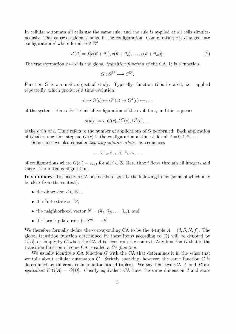
Example 1. (xor) Let d = 1, S = 0, 1, N = (0, 1) and f : 0, 12 −→ 0, 1 be

f(a, b) = a + b (mod 2).

The cells form a line, indexed by Z. Each cell changes its state by adding the state of itsright neighbor to its own old state modulo 2. This is known as the ”exclusive or” (xor) logicoperation.

Consider, for example, the initial configuration c0 where c0(0) = 1 and c0(i) = 0 forall i 6= 0, i.e. a single cell is in state 1. Then c1 = G(c0) has c1(0) = c1(−1) = 1 andc2(i) = 0 for all i 6= −1, 0. Continuing likewise, we get the time evolution c2 = G(c1),c3 = G(c2) etc. Figure 3 shows a diagram where we have drawn configurations as horizontalrows of states and depicted values 0 and 1 by white and black squares as we’ll typically doin our examples. The topmost row shows the initial configuration c0, and the following rowsrepresent consecutive elements of the orbit orb(c0). Time increases downwards.

?

Time

Figure 3: The space-time diagram of the xor CA of Example 1 starting from an initialconfiguration with a single cell in state 1.

¤

A space-time diagram is a pictorial representation of an orbit, similar to the one shown inExample 1 above. In the case of one-dimensional CA configurations are drawn as horizontallines of colors, each state represented by its own color. Configuration G(c) is drawn under c,so time flows downwards. The topmost row represents the initial configuration. The space-time diagram of the orbit of c hence fills the lower half plane. In contrast, the space-timediagrams associated with two-way infinite orbits fill the whole plane since there is no initialtime.

6

More generally, a space-time diagram of a d-dimensional CA is a (d + 1)-dimensional“drawing” where d dimensions represent space and the additional dimension is used fortime. Time gets values in N or Z depending on whether the diagram is for an orbit withan initial configuration or for a two-way infinite orbit. In the first case, the diagram is anelement of SZ

d×N, and in the second case it belongs to SZd×Z.

Following terminology is used: A configuration c is

• a fixed point of G if G(c) = c.

• (temporally) periodic if Gt(c) = c for some t ∈ Z+. Any t satisfying Gt(c) = c is calleda period of c and the smallest such t is the least period of c.

• eventually fixed if there is n ∈ N such that Gn+1(c) = Gn(c), that is, Gn(c) is a fixedpoint for some n.

• eventually (temporally) periodic if there is n ∈ N and t ∈ Z+ such that Gn+t(c) = Gn(c),that is, Gn(c) is periodic for some n.

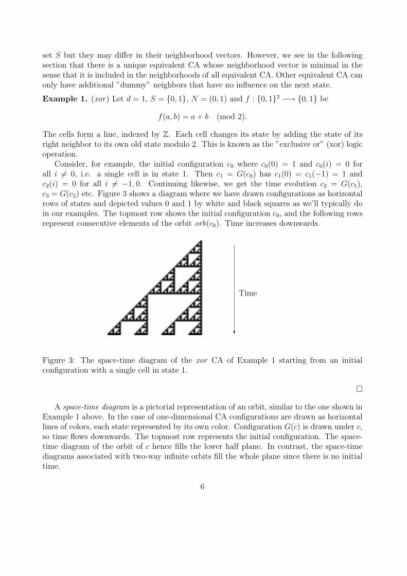
Analogous terminology is used for orbits. A one- or two-way infinite orbit is a fixedpoint orbit if all configurations it contains are fixed points (i.e. the orbit consists of copiesof the same fixed point configuration). It is periodic if it only contains temporally periodicconfigurations, it is eventually fixed if it contains some fixed point configuration and itis eventually periodic if it contains a temporally periodic configuration. See Figure 4 forillustrations of these concepts on two-way infinite orbits. The figure shows parts of phasespaces of some CA. A phase space is the infinite directed graph whose vertices are theconfigurations and from each configuration c there is exactly one outgoing edge leading toG(c). Note that the phase space has uncountably many vertices, so we always show just asmall portion of it, e.g. to plot some orbits as in Figure 4.

(a) (b) (c) (d)

Figure 4: (a) a fixed point, (b) a periodic orbit, (c) an eventually fixed orbit and (d) aneventually periodic orbit.

As a final observation of this section we state the following simple fact:

Proposition 1 If G and H are CA functions, so is their composition G H. ¤

7

1.4 Neighborhoods

Let N = (~n1, ~n2, . . . , ~nm) be a d-dimensional neighborhood vector. For any ~n ∈ Zd we denote

N(~n) = (~n + ~n1, ~n + ~n2, . . . , ~n + ~nm),

and for any K ⊆ Zd we denote

N(K) = ~n + ~ni | ~n ∈ K and i = 1, 2, . . . , m .

In other words, N(~n) is the ordered sequence of the neighbors of cell ~n, while N(K) isthe unordered set of neighbors of cells in K. In particular, N(~n) is the unordered setof neighbors of cell ~n. Clearly N = N(~0), and N(~0) is the unordered set that containsthe elements of the neighborhood vector N . The order of the elements in N is essentiallyirrelevant: it only matters as the order in which the m input values are given in the localrule f : Sm −→ S. So when specifying a CA it is enough to give the unordered versionN(~0) of N , as long as we make the role of different neighbors clear in the description ofthe local rule.

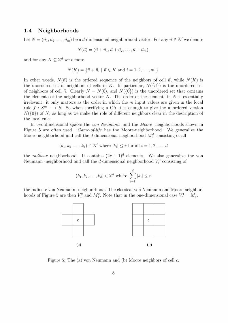
In two-dimensional spaces the von Neumann- and the Moore- neighborhoods shown inFigure 5 are often used. Game-of-life has the Moore-neighborhood. We generalize theMoore-neighborhood and call the d-dimensional neighborhood Md

r consisting of all

(k1, k2, . . . , kd) ∈ Zd where |ki| ≤ r for all i = 1, 2, . . . , d

the radius-r neighborhood. It contains (2r + 1)d elements. We also generalize the vonNeumann -neighborhood and call the d-dimensional neighborhood V d

r consisting of

(k1, k2, . . . , kd) ∈ Zd whered∑

i=1

|ki| ≤ r

the radius-r von Neumann -neighborhood. The classical von Neumann and Moore neighbor-hoods of Figure 5 are then V 2

1 and M21 . Note that in the one-dimensional case V 1

r = M1r .

(a) (b)

c c

Figure 5: The (a) von Neumann and (b) Moore neighbors of cell c.

8

The following, small neighborhoods will be sometimes used: The radius-12

neighborhoodconsists of all (k1, k2, . . . , kd) ∈ Zd where each ki ∈ 0, 1, and the radius-1

2von Neumann

-neighborhood consists of all (k1, k2, . . . , kd) ∈ Zd where at most one ki is 1 and all othersare 0. In the one-dimensional case these both consist of the cell and its immediate rightneighbor. The xor CA of Example 1 has the radius-1

2neighborhood.

Consider a CA with neighborhood vector N = (~n1, ~n2, . . . , ~nm) and local rule f : Sm −→S. We call ~nj a dummy neighbor if f(s1, . . . , sm) = f(t1, . . . , tm) whenever si = ti for alli 6= j. This means that the the j’th neighbor of a cell has no effect on the next state of thatcell, and hence ~nj can be removed from the neighborhood vector. We obtain an equivalentCA with m − 1 neighbors. Let us say a CA has minimal neighborhood if it has no dummyneighbors. By removing all dummy neighbors from any CA we obtain an equivalent CA thathas minimal neighborhood. This minimal neighborhood CA is unique:

Proposition 2 If A and B are equivalent CA and have minimal neighborhoods then A = B(up to reordering the neighbors in the neighborhood vector).

Proof. It is enough to show that the neighborhood vectors of A and B contain the sameelements. Let ~n be an arbitrary element of the neighborhood vector of A, that is, cell ~n is aneighbor of cell ~0 in A. Because A has no dummy neighbors there exist two configurationsc and e such that c(~n) 6= e(~n), c(~k) = e(~k) for all ~k 6= ~n and c′(~0) 6= e′(~0) where we havedenoted c′ = G(c) and e′ = G(e) and G is the global transition function of A. Since A andB are equivalent, G is also the transition function of B. This means that ~n has to be aneighbor of ~0 also in B, as otherwise we would have c′(~0) = e′(~0).

In the same way, every neighbor in B is also a neighbor in A. ¤

1.5 Elementary CA

Elementary CA are one-dimensional cellular automata with two states and radius-1 neigh-borhood: d = 1, S = 0, 1, N = (−1, 0, 1) and f : S3 −→ S. They differ from each otheronly in the choice of the local rule f . There are 256 elementary CA because the number ofdifferent local rules S3 −→ S is 28 = 256. Note, however, that some of the 256 elementaryrules are identical up to renaming the states or reversing right and left, so the number ofessentially different elementary rules is smaller, only 88.

Elementary rules were extensively studied and empirically classified by S.Wolfram in the1980’s. He introduced a naming scheme that has since become standard: Each elementaryrule is specified by an eight bit sequence

f(111) f(110) f(101) f(100) f(011) f(010) f(001) f(000)

where f is the local update rule of the CA. The bit sequence is the binary expansion of aninteger in the interval 0 . . . 255, called the Wolfram number of the CA.

9

Example 2. The 8 bit binary expansion of the decimal number 102 is 01100110 so theelementary CA with Wolfram number 102 has the local update rule

f(111) = 0, f(110) = 1, f(101) = 1, f(100) = 0,f(011) = 0, f(010) = 1, f(001) = 1, f(000) = 0,

This CA is equivalent to the xor CA of Example 1. ¤

Example 3.(rule 110 ) The 8 bit binary expansion of the decimal number 110 is 01101110so the elementary CA with Wolfram number 110 has the local update rule

f(111) = 0, f(110) = 1, f(101) = 1, f(100) = 0,f(011) = 1, f(010) = 1, f(001) = 1, f(000) = 0,

This CA has become known since it was recently proved to be computationally universal.The cover page of these notes contains a snapshot of the space-time diagram of rule 110started from a random initial configuration. ¤

Wolfram’s numbering scheme is easily generalized to larger neighborhoods and state sets.One-dimensional, radius-r CA with k states is identified by a number that contains k2r+1

base-k digits.S.Wolfram experimented in the 80’s with elementary CA, and based on empirical obser-

vations of their behavior on random initial configurations he classified them into four classes.These are known as Wolfram classes of CA. The definitions are not mathematically rigor-ous, and more precise classifications (which we’ll discuss later) have since been proposed.Wolfram defined the classes as follows:

(W1) Almost all initial configurations lead to the same uniform fixed point configuration,

(W2) Almost all initial configurations lead to a periodically repeating configuration,

(W3) Almost all initial configurations lead to essentially random looking behavior,

(W4) Localized structures with complex interactions emerge.

Figure 6 shows examples of typical space-time diagrams in each class. Wolfram conjecturedthat class (W4) cellular automata are computationally universal. In addition to rule 110also elementary CA 54 is in class (W4).

1.6 Finite configurations

Let s ∈ S be an arbitrary state. The s-support of configuration c ∈ SZd

is the set

supps(c) = ~n ∈ Zd | c(~n) 6= s

10

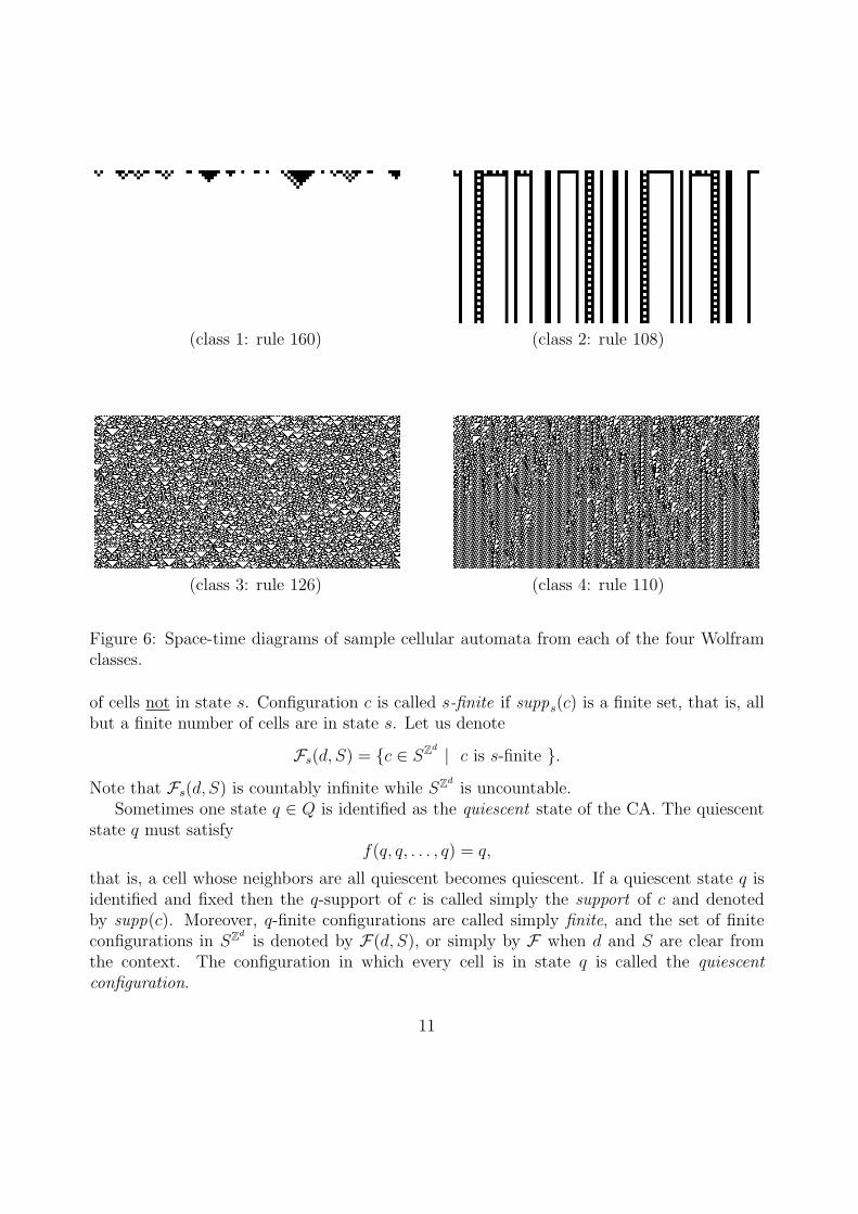
(class 1: rule 160) (class 2: rule 108)

(class 3: rule 126) (class 4: rule 110)

Figure 6: Space-time diagrams of sample cellular automata from each of the four Wolframclasses.

of cells not in state s. Configuration c is called s-finite if supps(c) is a finite set, that is, allbut a finite number of cells are in state s. Let us denote

Fs(d, S) = c ∈ SZd | c is s-finite .

Note that Fs(d, S) is countably infinite while SZd

is uncountable.Sometimes one state q ∈ Q is identified as the quiescent state of the CA. The quiescent

state q must satisfyf(q, q, . . . , q) = q,

that is, a cell whose neighbors are all quiescent becomes quiescent. If a quiescent state q isidentified and fixed then the q-support of c is called simply the support of c and denotedby supp(c). Moreover, q-finite configurations are called simply finite, and the set of finiteconfigurations in SZ

dis denoted by F(d, S), or simply by F when d and S are clear from

the context. The configuration in which every cell is in state q is called the quiescentconfiguration.

11

Clearly, if c is s-finite then G(c) is t-finite where t = f(s, s . . . , s). In particular, in thepresence of quiescent state q, finite configurations are mapped into finite configurations. Inthis case we denote by

GF : F −→ Fthe restriction of G on finite configurations.

In Example 1 (xor CA), we can name state 0 quiescent, in which case the space-timediagram in Figure 3 depicts a time-evolution according to GF . In Game-of-life (Section 1.2)the white square (no life) is taken as the quiescent state.

1.7 Periodic configurations

Let ~r ∈ Zd. Assuming a fixed and known state set S, the translation τ~r determined by ~ris the global transition function of the CA whose neighborhood contains only ~r and whoselocal rule is the identity function. In other words,

τ~r : SZd −→ SZ

d

maps c 7→ c′ where c′(~n) = c(~n + ~r) for all ~n ∈ SZd. It is obvious that for all ~r, ~s ∈ Zd and

k ∈ Z we haveτ~r τ~s = τ~r+~s, and

τ k~r = τk~r.

(3)

For each dimension i = 1, 2, . . . , d we call the translation by one cell down in dimensioni a shift and denote it by σi. More precisely, if we denote the i’th coordinate unit vector

~ei = (0, . . . , 0, 1, 0, . . . 0),

then σi = τ~ei. It follows from (3) that every translation is a composition of shifts. In the

one-dimensional case the only shift σ1 is called the left shift and we denote it simply by σ.The following proposition states an elementary but important property of cellular au-

tomata, based on the fact that all cells use the same local update rule:

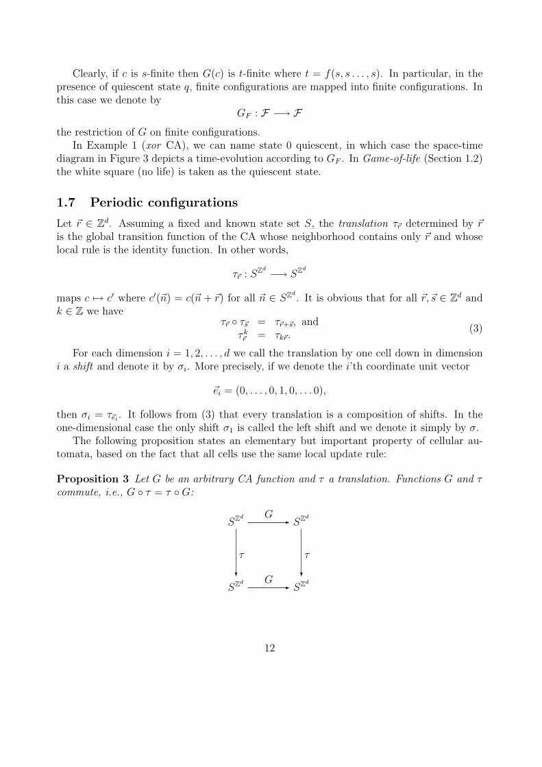
Proposition 3 Let G be an arbitrary CA function and τ a translation. Functions G and τcommute, i.e., G τ = τ G:

SZd G - SZ

d

SZd

τ

?G - SZ

d

τ

?

12

Proof. Let τ be the translation determined by ~r ∈ Zd, and let G be the transition functionof CA A = (d, S, N, f) where N is as in (1). For arbitrary c ∈ SZ

dand ~n ∈ Zd we have

τ(G(c))(~n) = G(c)(~n + ~r)

= f [c(~n + ~r + ~n1), c(~n + ~r + ~n2), . . . , c(~n + ~r + ~nm)]

= f [τ(c)(~n + ~n1), τ(c)(~n + ~n2), . . . , τ(c)(~n + ~nm)]

= G(τ(c))(~n),

so τ(G(c)) = G(τ(c)) and, furthermore, G τ = τ G. ¤

A configuration c ∈ SZd

is called ~r-periodic if

c(~n) = c(~n + ~r) for all ~n ∈ Zd.

Another way to say this is c = τ~r(c), i.e., c is invariant under the translation by ~r. Aconfiguration is called spatially periodic if it is ~r-periodic for some ~r 6= ~0.

A d-dimensional configuration is totally periodic if it is ~ri-periodic for some linearlyindependent ~r1, ~r2, . . . , ~rd ∈ Zd. It follows easily that a totally periodic configuration isσk

i -periodic for some k ∈ Z+ and all i = 1, 2, . . . , d. In other words, a totally periodicconfiguration consists of a hypercubic pattern(D, p) that is repeated periodically in each ofthe d-dimensions of the space. Let us denote by P(d, S) the set of totally periodic elementsof SZ

d, or if d and S are clear from the context we may simply denote P instead of P(d, S).

Set P is countably infinite.In the one-dimensional case there is no difference between spatial periodicity and total

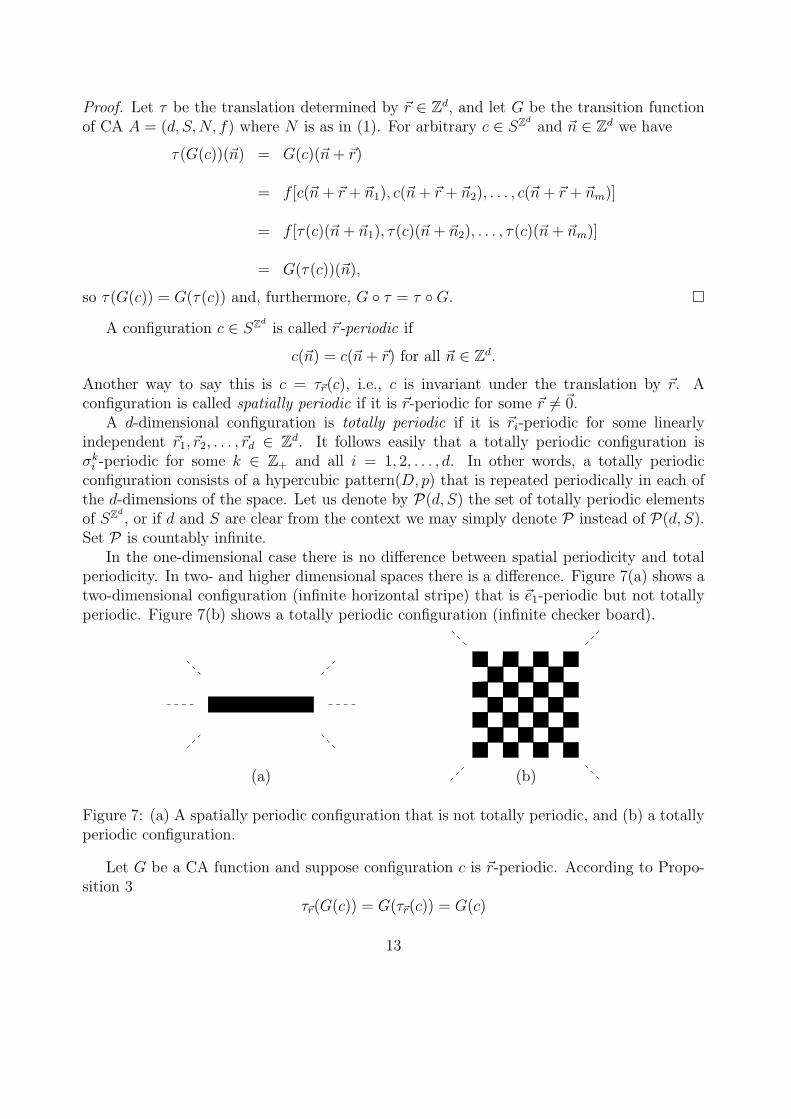
periodicity. In two- and higher dimensional spaces there is a difference. Figure 7(a) shows atwo-dimensional configuration (infinite horizontal stripe) that is ~e1-periodic but not totallyperiodic. Figure 7(b) shows a totally periodic configuration (infinite checker board).

(a) (b)

Figure 7: (a) A spatially periodic configuration that is not totally periodic, and (b) a totallyperiodic configuration.

Let G be a CA function and suppose configuration c is ~r-periodic. According to Propo-sition 3

τ~r(G(c)) = G(τ~r(c)) = G(c)

13

so also G(c) is ~r-periodic. In particular, if c is totally periodic then also G(c) is totallyperiodic. We denote by

GP : P −→ Pthe restriction of G on totally periodic configurations.

Finite configurations and periodic configurations are used in effective simulations of cel-lular automata on computers. Periodic configurations are often referred to as the periodicboundary conditions on a finite cellular array. For example, in the case d = 2 this is equiva-lent to running the CA on a torus that is obtained by ”gluing” together the opposite sidesof a rectangle. One should, however, keep in mind that the behavior of a CA can be quitedifferent on finite, periodic and general configurations, so experiments done with periodicboundary conditions may sometimes be misleading.

One final remark: Periodicity of a configuration defined in this section refers to spatialperiodicity. This should not be confused with temporal periodicity of a configuration definedat the end of Section 1.3, that is, the property that the configuration repeats itself underthe CA evolution.

1.8 Compactness principle

Topology plays an important role in the theory of cellular automata. The configuration spaceSZ

dcan be given a compact topology under which all CA functions G are continuous. We

delay the detailed discussion of this. Instead we prove two statements that capture essentialfeatures of the topological approach.

Consider an infinite sequence c1, c2, . . . of configurations, each ci ∈ SZd. We say that the

sequence converges and c ∈ SZd

is its limit if for every ~n ∈ Zd there exists some k ∈ Z+ suchthat ci(~n) = c(~n) for all i ≥ k. In other words: if we look at an arbitrary cell and browsethrough a converging sequence c1, c2, . . . then from some moment on we always see the samestate. It is obvious that if a limit exists it is unique, and we denote this limit by

limi→∞

ci.

A subsequence of c1, c2, . . . is another sequence ci1 , ci2 , . . . where i1 < i2 < . . .. A sub-sequence is hence obtained by picking infinitely many elements of the sequence, preservingtheir relative order. Obviously every subsequence of a converging sequence also convergesand has the same limit.

The first proposition states the compactness of the configuration space:

Proposition 4 Every sequence of configurations has a converging subsequence.

Proof. Let c1, c2, . . . be an arbitrary sequence, ci ∈ SZd. Let ~r1, ~r2, . . . be an enumeration of

elements of Zd. Let us choose indices i0 < i1 < i2 < i3 < . . . recursively as follows: i0 ∈ Z+

is arbitrary. Suppose then that ik−1 has been chosen and we want to choose ik for k ≥ 1.We choose ik to be the smallest integer that satisfies the following three conditions:

14

(1k) ik > ik−1,

(2k) cik(~rj) = cik−1(~rj) for all j = 1, 2, . . . k − 1.

(3k) There exist infinitely many indices i such that ci(~rj) = cik(~rj) for all j = 1, 2, . . . k.

Numbers ik that satisfy (1k)–(3k) always exist for the following reasons: Because condition(3k−1) was satisfied when ik−1 was chosen, we have infinitely many choices of ik that satisfy(2k). Set Sk is finite so there is a finite number of combinations of states that can appear incells ~r1, . . . , ~rk. Consequently, among the infinitely many indices ik that satisfy (2k) there areinfinitely many choices that also satisfy (3k). Some of them hence satisfy all requirements(1k)–(3k).

It follows from properties (2k) that ci1 , ci2 , . . . converges: For an arbitrary ~rk ∈ Zd all cij

for j ≥ k have the same state in cell ~rk. ¤

Note: The proof is essentially the same as the proof of weak Konig’s lemma which statesthat an infinite binary tree contains an infinite path. The proof did not require the axiomof choice. (The same result could also be briefly proved using Tychonoff’s theorem, but thatis equivalent to the axiom of choice.)

Our next proposition states a continuity property of CA functions:

Proposition 5 Let G be a CA function and c1, c2, . . . a converging sequence of configura-tions. Then also the sequence G(c1), G(c2), . . . converges and

limi→∞

G(ci) = G(c)

wherec = lim

i→∞ci.

Proof. Let G be the transition function of A = (d, S, N, f) where N is as in (1). Let ~n ∈ Zd

be arbitrary. Because c = limi→∞ ci we have that for every j = 1, 2, . . . , m there existskj ∈ Z+ such that

ci(~n + ~nj) = c(~n + ~nj) for all i ≥ kj.

Let k = maxk1, k2, . . . , km. Then if i ≥ k we have

G(ci)(~n) = f [ci(~n + ~n1), ci(~n + ~n2), . . . , ci(~n + ~nm)]

= f [c(~n + ~n1), c(~n + ~n2), . . . , c(~n + ~nm)]

= G(c)(~n).

Because ~n ∈ Zd was arbitrary, we have that G(c1), G(c2), . . . converges to G(c). ¤

15

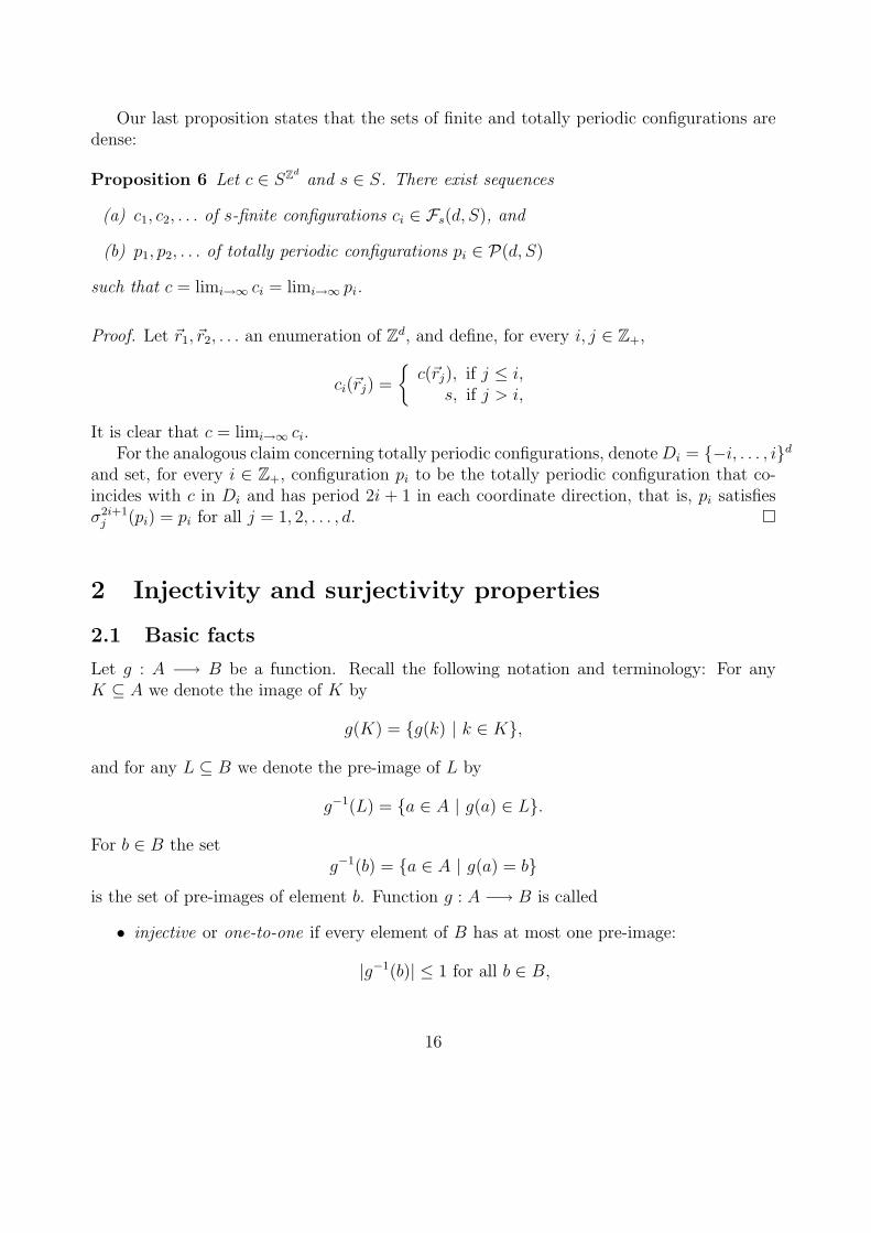
Our last proposition states that the sets of finite and totally periodic configurations aredense:

Proposition 6 Let c ∈ SZd

and s ∈ S. There exist sequences

(a) c1, c2, . . . of s-finite configurations ci ∈ Fs(d, S), and

(b) p1, p2, . . . of totally periodic configurations pi ∈ P(d, S)

such that c = limi→∞ ci = limi→∞ pi.

Proof. Let ~r1, ~r2, . . . an enumeration of Zd, and define, for every i, j ∈ Z+,

ci(~rj) =

c(~rj), if j ≤ i,

s, if j > i,

It is clear that c = limi→∞ ci.For the analogous claim concerning totally periodic configurations, denote Di = −i, . . . , id

and set, for every i ∈ Z+, configuration pi to be the totally periodic configuration that co-incides with c in Di and has period 2i + 1 in each coordinate direction, that is, pi satisfiesσ2i+1

j (pi) = pi for all j = 1, 2, . . . , d. ¤

2 Injectivity and surjectivity properties

2.1 Basic facts

Let g : A −→ B be a function. Recall the following notation and terminology: For anyK ⊆ A we denote the image of K by

g(K) = g(k) | k ∈ K,

and for any L ⊆ B we denote the pre-image of L by

g−1(L) = a ∈ A | g(a) ∈ L.

For b ∈ B the setg−1(b) = a ∈ A | g(a) = b

is the set of pre-images of element b. Function g : A −→ B is called

• injective or one-to-one if every element of B has at most one pre-image:

|g−1(b)| ≤ 1 for all b ∈ B,

16

• surjective or onto if every element of B has at least one pre-image:

|g−1(b)| ≥ 1 for all b ∈ B,

• bijective if it is both injective and surjective, that is, every element of B has exactlyone pre-image:

|g−1(b)| = 1 for all b ∈ B,

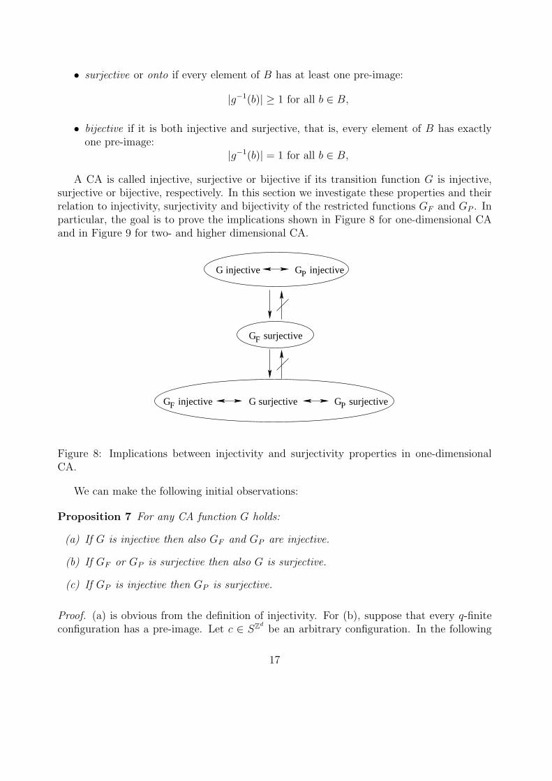
A CA is called injective, surjective or bijective if its transition function G is injective,surjective or bijective, respectively. In this section we investigate these properties and theirrelation to injectivity, surjectivity and bijectivity of the restricted functions GF and GP . Inparticular, the goal is to prove the implications shown in Figure 8 for one-dimensional CAand in Figure 9 for two- and higher dimensional CA.

G injective G injective

G surjective

G surjectiveG injective G surjective

P

F

F P

Figure 8: Implications between injectivity and surjectivity properties in one-dimensionalCA.

We can make the following initial observations:

Proposition 7 For any CA function G holds:

(a) If G is injective then also GF and GP are injective.

(b) If GF or GP is surjective then also G is surjective.

(c) If GP is injective then GP is surjective.

Proof. (a) is obvious from the definition of injectivity. For (b), suppose that every q-finiteconfiguration has a pre-image. Let c ∈ SZ

dbe an arbitrary configuration. In the following

17

G injective

G surjective

G surjectiveG injective

F

F

G injectiveP

G surjectiveP

?

?

?

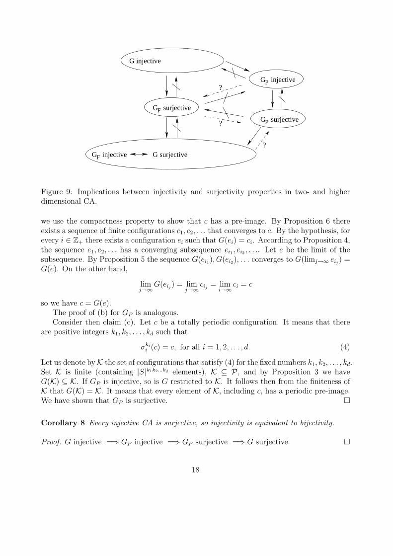
Figure 9: Implications between injectivity and surjectivity properties in two- and higherdimensional CA.

we use the compactness property to show that c has a pre-image. By Proposition 6 thereexists a sequence of finite configurations c1, c2, . . . that converges to c. By the hypothesis, forevery i ∈ Z+ there exists a configuration ei such that G(ei) = ci. According to Proposition 4,the sequence e1, e2, . . . has a converging subsequence ei1 , ei2 , . . .. Let e be the limit of thesubsequence. By Proposition 5 the sequence G(ei1), G(ei2), . . . converges to G(limj→∞ eij) =G(e). On the other hand,

limj→∞

G(eij) = limj→∞

cij = limi→∞

ci = c

so we have c = G(e).The proof of (b) for GP is analogous.Consider then claim (c). Let c be a totally periodic configuration. It means that there

are positive integers k1, k2, . . . , kd such that

σkii (c) = c, for all i = 1, 2, . . . , d. (4)

Let us denote byK the set of configurations that satisfy (4) for the fixed numbers k1, k2, . . . , kd.Set K is finite (containing |S|k1k2...kd elements), K ⊆ P , and by Proposition 3 we haveG(K) ⊆ K. If GP is injective, so is G restricted to K. It follows then from the finiteness ofK that G(K) = K. It means that every element of K, including c, has a periodic pre-image.We have shown that GP is surjective. ¤

Corollary 8 Every injective CA is surjective, so injectivity is equivalent to bijectivity.

Proof. G injective =⇒ GP injective =⇒ GP surjective =⇒ G surjective. ¤

18

2.2 Reversible CA

A cellular automaton function G is called reversible if it is bijective and the inverse functionG−1 is also a CA function. A cellular automaton A is called reversible if its global transitionfunction G is reversible. Then the CA computing G−1 is called the inverse automaton of A,and we denote it by A−1. We know from Proposition 2 that the inverse automaton is uniqueup to adding dummy neighbors and ordering of the neighbors. The inverse of A retraces theorbits of A backwards in time.

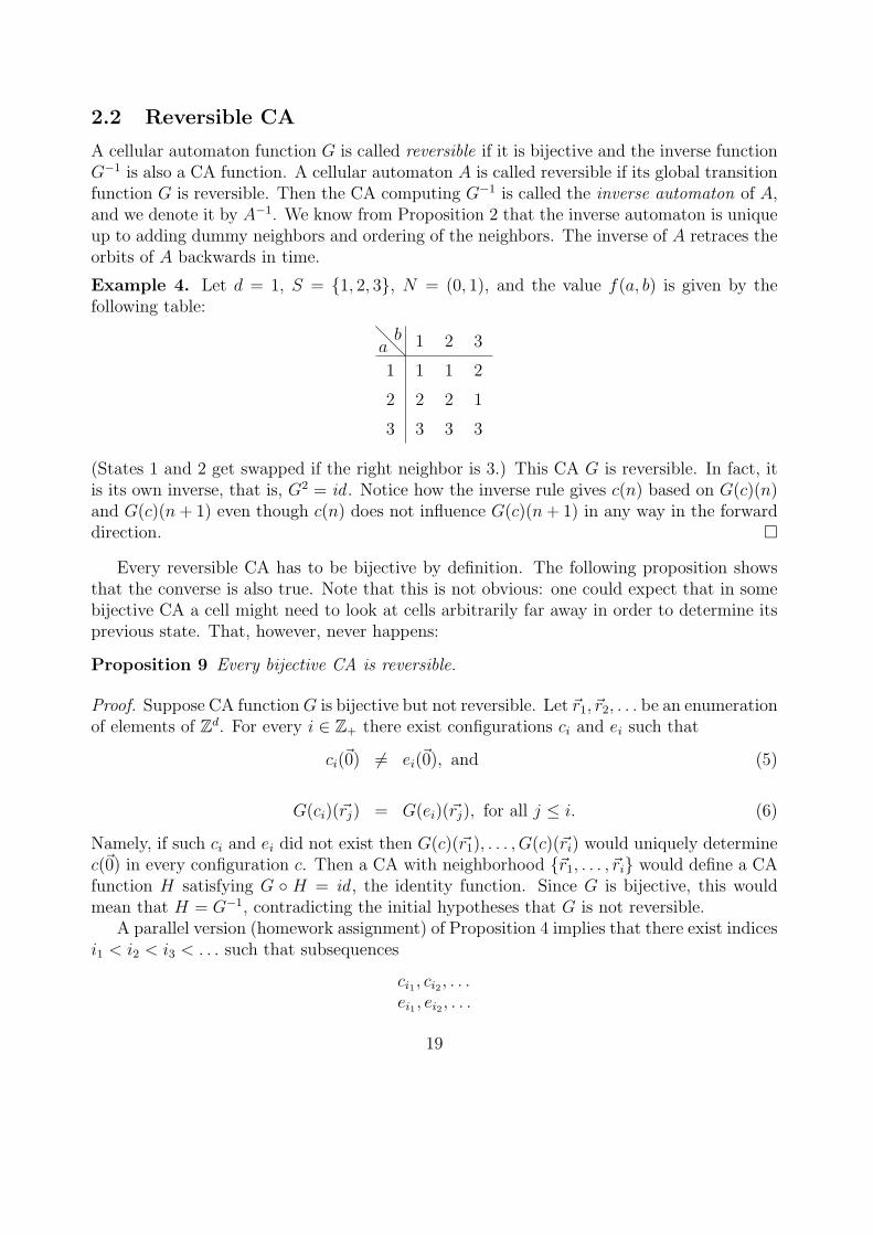
Example 4. Let d = 1, S = 1, 2, 3, N = (0, 1), and the value f(a, b) is given by thefollowing table:

@@b

a 1 2 3

1

2

3

1 1 2

2 2 1

3 3 3

(States 1 and 2 get swapped if the right neighbor is 3.) This CA G is reversible. In fact, itis its own inverse, that is, G2 = id . Notice how the inverse rule gives c(n) based on G(c)(n)and G(c)(n + 1) even though c(n) does not influence G(c)(n + 1) in any way in the forwarddirection. ¤

Every reversible CA has to be bijective by definition. The following proposition showsthat the converse is also true. Note that this is not obvious: one could expect that in somebijective CA a cell might need to look at cells arbitrarily far away in order to determine itsprevious state. That, however, never happens:

Proposition 9 Every bijective CA is reversible.

Proof. Suppose CA function G is bijective but not reversible. Let ~r1, ~r2, . . . be an enumerationof elements of Zd. For every i ∈ Z+ there exist configurations ci and ei such that

ci(~0) 6= ei(~0), and (5)

G(ci)(~rj) = G(ei)(~rj), for all j ≤ i. (6)

Namely, if such ci and ei did not exist then G(c)(~r1), . . . , G(c)(~ri) would uniquely determinec(~0) in every configuration c. Then a CA with neighborhood ~r1, . . . , ~ri would define a CAfunction H satisfying G H = id , the identity function. Since G is bijective, this wouldmean that H = G−1, contradicting the initial hypotheses that G is not reversible.

A parallel version (homework assignment) of Proposition 4 implies that there exist indicesi1 < i2 < i3 < . . . such that subsequences

ci1 , ci2 , . . .ei1 , ei2 , . . .

19

both converge. Letc = lim

j→∞cij ,

e = limj→∞

eij

be their limits. According to (5) we have cij(~0) 6= eij(~0) for every j, so c(~0) 6= e(~0). Thismeans that c 6= e.

On the other hand, it follows from the continuity property (Proposition 5) that sequences

G(ci1), G(ci2), . . .G(ei1), G(ei2), . . .

converge, andlimj→∞

G(cij) = G(c),

limj→∞

G(eij) = G(e).

But it follows from (6) that the limits must be same, so G(c) = G(e), which contradicts thebijectivity of G.

¤

By Proposition 9 and Corollary 8, injectivity, bijectivity and reversibility are equivalentconcepts on cellular automata.

2.3 Balance in surjective CA

A configuration c is a Garden-of-Eden configuration (GOE) if it has no pre-images, i.e. ifG−1(c) is empty. A CA has Garden-of-Eden configurations if and only if the CA is notsurjective.

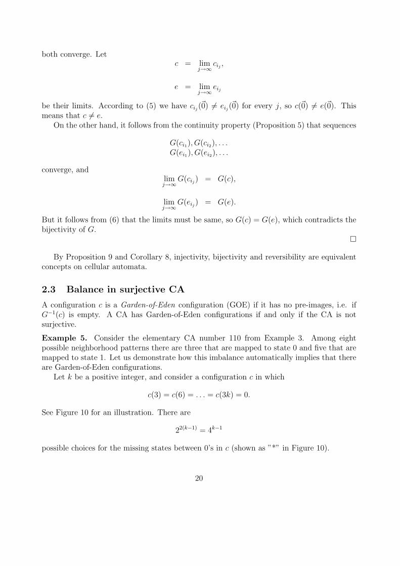
Example 5. Consider the elementary CA number 110 from Example 3. Among eightpossible neighborhood patterns there are three that are mapped to state 0 and five that aremapped to state 1. Let us demonstrate how this imbalance automatically implies that thereare Garden-of-Eden configurations.

Let k be a positive integer, and consider a configuration c in which

c(3) = c(6) = . . . = c(3k) = 0.

See Figure 10 for an illustration. There are

22(k−1) = 4k−1

possible choices for the missing states between 0’s in c (shown as ”*” in Figure 10).

20

*

x x x x x x x x x x x x x x x

0 * 0 * * 0*c

e

0 * * 0 *

Figure 10: Illustration of the configuration c and its pre-image e in Example 5.

In a pre-image e of c the three state segments e(i−1), e(i), e(i+1) are mapped into state0 by the local rule f , for every i = 1, 2, . . . , k. Since |f−1(0)| = 3 there are exactly 3k choicesof these segments.

If k is sufficiently large then 3k < 4k−1. This means that that some choice of c does nothave a corresponding pre-image e. Therefore the CA is not surjective.

Alternatively, one could show the non-surjectivity of rule 110 by directly verifying thatany configuration containing pattern 01010 is a Garden-of-Eden.

¤

In this section we generalize the previous example. We need first to define the conceptof a (finite) pattern. A pattern

p = (D, g)

is a partial configuration where D ⊆ Zd is the domain of p and g : D −→ S is a mappingassigning a state to each cell in the domain. Pattern p is finite if D is a finite set. Note thatconfigurations are patterns whose domain is the entire space Zd. If τ is a translation of Zd

then τ(p) is the pattern p′ = (D′, g′) where D′ = τ(D) and g = τ g′. We then say that pand p′ are translated copies of each other.

If p1 = (D1, g1) and p2 = (D2, g2) are two patterns we say that p1 is a subpattern of p2

if D1 ⊆ D2 and g1(~n) = g2(~n) for all ~n ∈ D1. We say that p2 contains a copy of p1 if sometranslated copy of p1 is a subpattern of p2. Patterns p1 and p2 are disjoint if D1 ∩D2 = ∅.

Let G be CA function specified by CA A = (d, S,N, f), where N is given by (1). Letp = (D, g) be a pattern, and let D′ ⊆ Zd a domain such that N(D′) ⊆ D, that is, all neighborsof all cells of D′ are in D. An application of the local rule f on pattern p determines newstates for all cells in domain D′. We obtain a pattern p′ = (D′, g′) where for all ~n ∈ D′

g′(~n) = f [g(~n + ~n1), g(~n + ~n2), . . . , g(~n + ~nm)].

The mapping p 7→ p′ will be denoted by G(D→D′), or simply by G when the domains Dand D′ are clear from the context and there is no risk of confusion. Note that the globaltransition function of the CA is G(Zd→Zd).

A finite pattern without a pre-image is called an orphan. In other words, patternp′ = (D′, g′) is an orphan if G(D→D′)(p) 6= p′ for all p = (D, g) with domain D = N(D′).Clearly any configuration that contains a copy of an orphan is a Garden-of-Eden configu-ration. Also the converse is true, as stated in the next proposition. The proof is similar toProposition 7(b).

21

Proposition 10 Every Garden-of-Eden configuration has a subpattern that is an orphan.Hence, a cellular automaton is non-surjective if and only if there exists an orphan.

Proof. Let c ∈ SZd

be a Garden-of-Eden configuration, and suppose that none of its subpat-terns is an orphan. Let ~r1, ~r2, . . . be an enumeration of elements of Zd and denote, for everyj ∈ Z+,

Dj = ~r1, ~r2, . . . , ~rj.Since the subpattern of c with domain Dj is not an orphan, there exists a configuration

cj ∈ SZd

such that G(cj) agrees with c in domain Dj. This implies that the sequenceG(c1), G(c2), . . . converges to c. By compactness (Proposition 4) the sequence c1, c2, . . . hasa converging subsequence ci1 , ci2 , . . ., with some limit e ∈ SZ

d. By the continuity of G

(Proposition 5) the sequence G(ci1), G(ci2), . . . converges to G(e). On the other hand,

limj→∞

G(cij) = limi→∞

G(ci) = c.

So we have c = G(e), which means that c is not a GOE. ¤

The following lemma is a technical result that will be needed in this and the next section:

Lemma 11 For all d, n, s, r ∈ Z+ there exists k ∈ Z+ such that

(snd − 1

)kd

< s(kn−2r)d

.

Proof. A homework assignment. ¤

The d-dimensional hypercube of size nd determined by corner (k1, k2, . . . , kd) ∈ Zd is thefinite domain

D = (x1, x2, . . . , xd) ∈ Zd | ki ≤ xi < ki + n for all i = 1, 2, . . . , d .

Patterns with hypercubic domains will be extensively used in proofs below. Now we areready to state and prove the balance property of surjective CA:

Proposition 12 Let A = (d, S, N, f) be a surjective CA, and let D,D′ ⊆ Zd be finitedomains such that N(D′) ⊆ D. Then for every pattern p′ = (D′, g′) the number of patternsp = (D, g) such that

G(D→D′)(p) = p′

is s|D|−|D′| where s = |S| is the number of states.

22

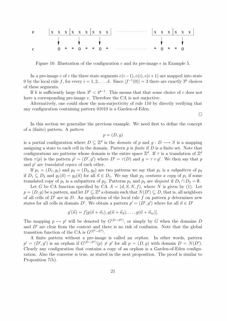
Proof. Suppose there exists p′ such that the number of pre-image patterns p in domainD is t 6= s|D|−|D

′|. Let us first show that we can assume that the domains D and D′ arehypercubes, with D′ centered inside D.

Let E, E ′ ⊆ Zd be arbitrary finite domains such that D ⊆ E, D′ ⊆ E ′ and N(E ′) ⊆ E. Inparticular, for sufficiently large n and r we can choose E and E ′ to be cocentric hypercubesof size nd and (n− 2r)d, respectively. There are s|E

′|−|D′| patterns in domain E ′ that have p′

as a subpattern (one can choose arbitrary states in the cells in E ′ \D′, a shaded region inFigure 11), and they have t · s|E|−|D| pre-image patterns in domain E (obtained from the tpre-images of p′ by choosing arbitrary states in the remaining cells in E \D, also shaded inFigure 11). If each pattern in domain E ′ would have s|E|−|E

′| pre-images in domain E, wewould have

s|E′|−|D′| · s|E|−|E′| = t · s|E|−|D|.

This implies t = s|D|−|D′|, a contradiction. We conclude that there is a pattern in domain E ′

that has an ”imbalanced” number of pre-images in domain E.

D E’

E

D’

Figure 11: Domains D, D′, E and E ′.

In the following we hence assume that D and D′ are cocentric hypercubes of size nd and(n − 2r)d, respectively. We also assume that the number t of pre-images of p′ = (D′, g′) indomain D satisfies

t < s|D|−|D′|.

Namely, the total number of patterns in domains D and D′ are s|D| and s|D′|, respectively,

so if every pattern in domain D′ would have at least s|D|−|D′| pre-images in domain D,

then every pattern would necessarily have exactly s|D|−|D′| pre-images, contradicting the

assumption that p′ has an imbalanced number of pre-images.The main part of the proof that follows is similar to Example 5. Let k ∈ Z+ be arbitrary.

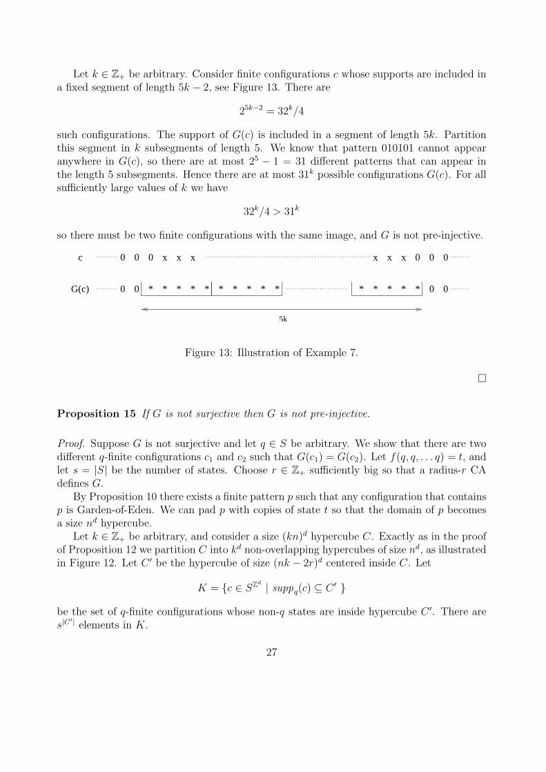
Consider a domain C that is a hypercube of size (kn)d, partitioned into kd non-overlappinghypercubes of size nd. See Figure 12 for an illustration. Let C ′ be the hypercube of size(nk − 2r)d centered inside C, and let us denote by A the set of finite patterns with domainC ′ such that each of the kd shaded domains in Figure 12 contain a copy of pattern p′. The

23

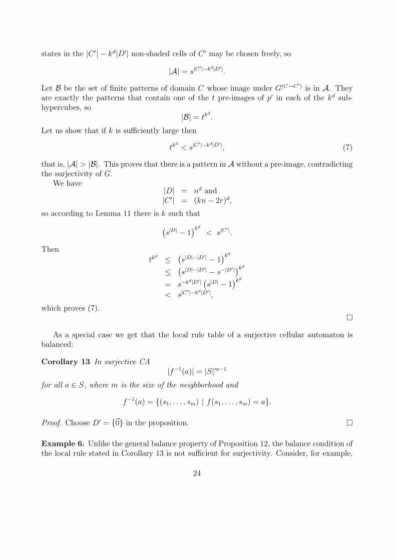
states in the |C ′| − kd|D′| non-shaded cells of C ′ may be chosen freely, so

|A| = s|C′|−kd|D′|.

Let B be the set of finite patterns of domain C whose image under G(C→C′) is in A. Theyare exactly the patterns that contain one of the t pre-images of p′ in each of the kd sub-hypercubes, so

|B| = tkd

.

Let us show that if k is sufficiently large then

tkd

< s|C′|−kd|D′|, (7)

that is, |A| > |B|. This proves that there is a pattern in A without a pre-image, contradictingthe surjectivity of G.

We have|D| = nd and|C ′| = (kn− 2r)d,

so according to Lemma 11 there is k such that

(s|D| − 1

)kd

< s|C′|.

Then

tkd ≤ (

s|D|−|D′| − 1

)kd

≤ (s|D|−|D

′| − s−|D′|)kd

= s−kd|D′| (s|D| − 1)kd

< s|C′|−kd|D′|,

which proves (7).¤

As a special case we get that the local rule table of a surjective cellular automaton isbalanced:

Corollary 13 In surjective CA|f−1(a)| = |S|m−1

for all a ∈ S, where m is the size of the neighborhood and

f−1(a) = (s1, . . . , sm) | f(s1, . . . , sm) = a.

Proof. Choose D′ = ~0 in the proposition. ¤

Example 6. Unlike the general balance property of Proposition 12, the balance condition ofthe local rule stated in Corollary 13 is not sufficient for surjectivity. Consider, for example,

24

n

n

n n n n

kn

r

kn

r

n

Figure 12: Illustration for the proofs of Propositions 12, 15 and 18.

the elementary CA number 232. It is the majority CA: f(a, b, c) = 1 if and only if a+b+c ≥ 2.Its rule table is balanced because 000, 001, 010, 100 map to 0 and 111, 110, 101, 011 map to1.

However, the majority CA is not balanced on longer patterns and hence it is not surjec-tive: Any pattern of length four that contains at most one state 1 is mapped to 00, so 00 hasat least 5 pre-images of length four. Balanceness would require this number of pre-imagesto be 4.

¤

2.4 Garden-of-Eden -theorem

One of the oldest results in cellular automata theory is the so-called Garden-of-Eden -theoremthat states that there are Garden-of-Eden configurations if and only if there are differentfinite configurations with the same image. In other words: G is surjective if and only if GF

is injective. The two directions of the statement were proved by E.F.Moore in 1962 andJ.Myhill in 1963.

A natural way to state the Garden-of-Eden -theorem without any reference to a quiescentstate is in terms of pre-injectivity. Configurations c1 and c2 are called asymptotic if the set

diff (c1, c2) = ~n ∈ Zd | c1(~n) 6= c2(~n)

25

of positions where c1 and c2 differ is finite. Cellular automaton G is pre-injective if forany asymptotic c1 and c2 holds c1 6= c2 =⇒ G(c1) 6= G(c2). Clearly all injective CA arepre-injective.

The following proposition shows that for pre-injectivity it is enough that the CA is one-to-one among c-asymptotic configurations, for any fixed configuration c. In particular – bychoosing as c any q-finite configuration – we see that pre-injectivity is equivalent to injectivityof GF .

Proposition 14 Let c ∈ SZd

be arbitrary. Cellular automaton G is pre-injective if and onlyif it is injective in the domain

asymp(c) = e ∈ SZd | c and e are asymptotic .

Proof. It is clear that pre-injectivity implies injectivity in domain asymp(c). For the conversedirection, suppose that G is injective in asymp(c), and let c1 and c2 be two asymptoticconfigurations, c1 6= c2. Assume that we could have G(c1) = G(c2).

Let N ⊆ Zd be the set of the elements of the neighborhood vector. We may assume~0 ∈ N : if not, we simply add ~0 as a dummy neighbor. Denote by

A = diff (c1, c2)−N

the set of cells that have a neighbor in diff (c1, c2), and by

B = A + N = diff (c1, c2) + N −N

the neighborhood of A. Clearly A and B are finite sets.Consider the configurations e1 and e2 where ei(~n) = ci(~n) for all ~n ∈ B, and ei(~n) = c(~n)

for ~n 6∈ B. Because c1 6= c2 and diff (c1, c2) ⊆ B, we also have e1 6= e2. But G(e1) = G(e2)because

• for ~n ∈ A the neighborhood of ~n is inside B, so G(e1)(~n) = G(c1)(~n) = G(c2)(~n) =G(e2)(~n), and

• for ~n 6∈ A, the neighborhood of ~n does not contain elements of diff (c1, c2), so configura-tions e1 and e2 are identical in the neighborhood of cell ~n. Hence G(e1)(~n) = G(e2)(~n).

Configurations e1 and e2 are asymptotic to c, which contradicts the injectivity of G in theset asymp(c). ¤

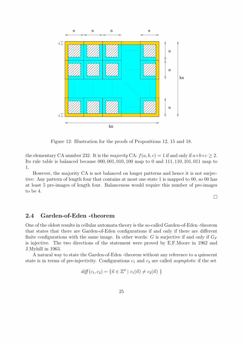
Example 7. As in the previous section, we start by illustrating the proof of the Garden-of-Eden -theorem using elementary rule 110. We know from Example 5 that rule 110 is notsurjective. In fact, finite pattern 01010 has no pre-image. Let us demonstrate that theremust exist different 0-finite configurations c and e such that G(c) = G(e).

26

Let k ∈ Z+ be arbitrary. Consider finite configurations c whose supports are included ina fixed segment of length 5k − 2, see Figure 13. There are

25k−2 = 32k/4

such configurations. The support of G(c) is included in a segment of length 5k. Partitionthis segment in k subsegments of length 5. We know that pattern 010101 cannot appearanywhere in G(c), so there are at most 25 − 1 = 31 different patterns that can appear inthe length 5 subsegments. Hence there are at most 31k possible configurations G(c). For allsufficiently large values of k we have

32k/4 > 31k

so there must be two finite configurations with the same image, and G is not pre-injective.

5k

* * * * * * * * * * * * * * *

000 0 0 0

0 000

x x x xxxc

G(c)

Figure 13: Illustration of Example 7.

¤

Proposition 15 If G is not surjective then G is not pre-injective.

Proof. Suppose G is not surjective and let q ∈ S be arbitrary. We show that there are twodifferent q-finite configurations c1 and c2 such that G(c1) = G(c2). Let f(q, q, . . . q) = t, andlet s = |S| be the number of states. Choose r ∈ Z+ sufficiently big so that a radius-r CAdefines G.

By Proposition 10 there exists a finite pattern p such that any configuration that containsp is Garden-of-Eden. We can pad p with copies of state t so that the domain of p becomesa size nd hypercube.

Let k ∈ Z+ be arbitrary, and consider a size (kn)d hypercube C. Exactly as in the proofof Proposition 12 we partition C into kd non-overlapping hypercubes of size nd, as illustratedin Figure 12. Let C ′ be the hypercube of size (nk − 2r)d centered inside C. Let

K = c ∈ SZd | suppq(c) ⊆ C ′

be the set of q-finite configurations whose non-q states are inside hypercube C ′. There ares|C

′| elements in K.

27

The t-support of G(c) for every c ∈ K is inside C. Moreover, G(c) cannot contain patternp in any of the kd sub-hypercubes of size nd. It means that there are at most

(snd − 1

)kd

possible configurations G(c). But according to Lemma 11 for some k

(snd − 1

)kd

< s(kn−2r)d

= s|C′| = |K|,

so there are c1, c2 ∈ K such that c1 6= c2 while G(c1) = G(c2). ¤

Corollary 16 If GF is injective then G is surjective.

Proof. If GF is injective then G is pre-injective by Proposition 14, and then by Proposition 15it is surjective. ¤

Note that the implication chain

G injective =⇒ G pre-injective =⇒ G surjective

provides a second proof of Corollary 8 that uses asymptotic pairs of configurations insteadof periodic configurations.

Corollary 17 If G is injective then GF is surjective.

Proof. If G is injective then it is reversible by Proposition 9 and Corollary 8. If q is thequiescent state of G then it is also quiescent in the inverse CA, that is, the local rule g ofthe inverse CA maps g(q, q, . . . , q) = q. Hence, if c is a finite configuration, also e = G−1(c)is finite and G(e) = c, so c has a finite pre-image. ¤

Next we turn to the other direction of the Garden-of-Eden -theorem. Again, we startwith a one-dimensional example that indicates the proof idea.

Example 8. Consider again rule 110. The 0-finite configurations

c1 = . . . 000011010000 . . .c2 = . . . 000010110000 . . .

have the same image. Let us demonstrate how this implies that rule 110 is not surjective.(Of course we already know this fact form the prior examples.)

Extract patterns p1 = 00110100 and p2 = 00101100 of length eight from c1 and c2, re-spectively. Both patterns are mapped into the same pattern 111110 of length six. Moreover,p1 and p2 have a boundary of width 2 on both sides where they are identical with each other.

28

Since rule 110 uses radius-1 neighborhood, one can replace in any configuration c pattern p1

by p2 or vice versa without affecting G(c).Let k ∈ Z+, and consider a segment of 8k cells. It consists of k segments of length 8. Any

pattern of length 8k − 2 that has a pre-image of length 8k also has a pre-image where noneof the k subsegments of length 8 contains pattern p1. Namely, all such p1 can be replaced byp2. This means that at most (28− 1)k = 255k patterns of length 8k− 2 can have pre-images.On the other hand there are 28k−2 = 256k/4 such patterns, and for large values of k

256k/4 > 255k,

so some patterns do not have a pre-image. ¤

Proposition 18 If G is not pre-injective then G has Garden-of-Eden configurations.

Proof. Suppose c1 and c2 are asymptotic, c1 6= c2 but G(c1) = G(c2). Let r be sufficientlylarge so that G is defined by a radius- r

2cellular automaton. Choose n sufficiently large so

that there is a size (n− 2r)d hypercube D′ containing all cells where c1 and c2 differ, that is,

diff (c1, c2) ⊆ D′.

Let D be the size nd hypercube around D′ that is cocentric with D′, and let p1 = (D, g1)and p2 = (D, g2) be the subpatterns of c1 and c2 with domain D, respectively.

In any configuration c that has subpattern p1 we can replace that subpattern p1 by p2

without affecting G(c). Indeed, those cells ~n whose neighborhood does not contain elementsof diff (c1, c2) do not see any change in their neighborhood. Those cells ~n whose neighborhoodcontains elements of diff (c1, c2) are within distance r

2of D′, so their neighborhood is entirely

inside D. ThereforeG(c)(~n) = G(c1)(~n) = G(c2)(~n) = G(c′)(~n)

where c′ is the configuration obtained from c by replacing subpattern p1 by p2.As in the proofs of Propositions 12 and 15, let k ∈ Z+ and let C be a hypercube of size

(kn)d, consisting of kd non-overlapping sub-hypercubes of size nd. Let C ′ be the hypercubeof size (kn − 2r)d centered inside C, see Figure 12. If G is surjective then every patternwith domain C ′ has a pre-image in domain C, and based on the discussion above, it has apre-image where none of the kd sub-hypercubes of size nd contains a copy of p1. But thereare only

(s|D| − 1

)kd

=(snd − 1

)kd

such patterns in domain C, while there are

s(kn−2r)d

patterns in domain C ′. It follows from Lemma 11 that some pattern does not have a pre-image.

¤

29

Corollary 19 If G is surjective then GF is injective. ¤

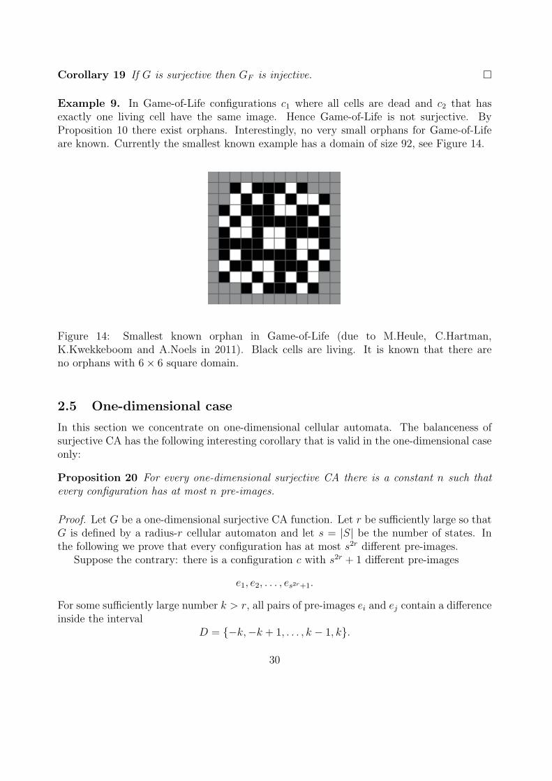
Example 9. In Game-of-Life configurations c1 where all cells are dead and c2 that hasexactly one living cell have the same image. Hence Game-of-Life is not surjective. ByProposition 10 there exist orphans. Interestingly, no very small orphans for Game-of-Lifeare known. Currently the smallest known example has a domain of size 92, see Figure 14.

Figure 14: Smallest known orphan in Game-of-Life (due to M.Heule, C.Hartman,K.Kwekkeboom and A.Noels in 2011). Black cells are living. It is known that there areno orphans with 6× 6 square domain.

2.5 One-dimensional case

In this section we concentrate on one-dimensional cellular automata. The balanceness ofsurjective CA has the following interesting corollary that is valid in the one-dimensional caseonly:

Proposition 20 For every one-dimensional surjective CA there is a constant n such thatevery configuration has at most n pre-images.

Proof. Let G be a one-dimensional surjective CA function. Let r be sufficiently large so thatG is defined by a radius-r cellular automaton and let s = |S| be the number of states. Inthe following we prove that every configuration has at most s2r different pre-images.

Suppose the contrary: there is a configuration c with s2r + 1 different pre-images

e1, e2, . . . , es2r+1.

For some sufficiently large number k > r, all pairs of pre-images ei and ej contain a differenceinside the interval

D = −k,−k + 1, . . . , k − 1, k.

30

In other words, for all i, j with 1 ≤ i < j ≤ s2r + 1 there is l ∈ D such that ei(l) 6= ej(l).But this contradicts Proposition 12 since we now have a pattern with domain

D′ = −k + r,−k + r + 1, . . . , k − r

that hass2r + 1 > s|D|−|D

′|

different pre-images in domain D. ¤

Corollary 21 Let G be a one-dimensional surjective CA function. If c ∈ SZ is not periodicthen G(c) is not periodic either. In particular, GP is surjective.

Proof. Suppose G(c) is periodic, so that σn(G(c)) = G(c) for some n ∈ Z+. Then for everyi ∈ Z

G(σin(c)) = σin(G(c)) = G(c),

so σin(c) is a pre-image of G(c). By Proposition 20 configuration G(c) has a finite numberof pre-images so

σi1n(c) = σi2n(c)

for some i1 < i2. But then c is periodic with period (i2− i1)n. It follows that all pre-imagesof periodic configurations are periodic. ¤

Proposition 20 and Corollary 21 do not hold for two-dimensional surjective cellular au-tomata as shown by the following example:

Example 10. Consider the two-dimensional xor CA with radius-12

neighborhood: d = 2,S = 0, 1,

N = [(0, 0), (0, 1), (1, 0), (1, 1)]

and the local rule f : 0, 14 −→ 0, 1 is

f(a, b, c, d) =

0, if a + b + c + d is even,1, if a + b + c + d is odd.

This CA is surjective: otherwise there would be two different finite configurations c, e ∈0, 1Z2

with the same image G(c) = G(e), see Proposition 15. If (x, y) ∈ Z2 is a cell wherec(x, y) 6= e(x, y) then it follows from the local rule of the CA that c(x′, y′) 6= e(x′, y′) for(x′, y′) = (x + 1, y), (x, y + 1) or (x + 1, y + 1). In any case x′ + y′ > x + y, which impliesthat the set of cells where c and e differ cannot be a finite set.

Even though the CA is surjective the (totally periodic) quiescent configuration c0 in whichall cells are in state 0 has uncountably many pre-images. For example, any configuration cthat consists of horizontal stripes, i.e.

c(i, k) = c(j, k)

31

for all i, j, k ∈ Z, is a pre-image of c0. Many of these pre-images are not totally periodic.However, the second part of Corollary 21 is not refuted by this example since GP is surjective.It is not known whether the surjectivity of G always implies the surjectivity of GP in two-and higher dimensional CA. ¤

The following proposition states a converse of Proposition 20. This statement is valid inany dimension:

Proposition 22 If G is a non-surjective CA then there is a totally periodic configurationc ∈ P that has infinitely (even uncountably) many pre-images.

Proof. Homework.

We can, in fact, be more specific about the structure of the pre-images in surjectiveone-dimensional CA. Let us call two one-dimensional configurations c, e ∈ SZ positivelyasymptotic (negatively asymptotic) if c(i) = e(i) for all sufficiently large (all sufficiently small,respectively) i ∈ Z. Let us call c and e positively n-separated (negatively n-separated) if for allsufficiently large (sufficiently small, respectively) i ∈ Z there is j ∈ i, i+1, i+2, . . . , i+n−1such that c(j) 6= e(j). We say that c and e are positively separated (negatively separated)if they are positively n-separated (negatively n-separated, respectively) for some n ∈ Z+.Configurations c and e are totally n-separated if for all i ∈ Z there is j ∈ i, i+1, i+2, . . . , i+n−1 such that c(j) 6= e(j), and c and e are totally separated if they are totally n-separatedfor some n. Clearly c and e are totally separated if and only if they are both positively andnegatively separated (but the separation parameter n may be different).

Also the following terminology related to one-dimensional neighborhoods will be used:Number m is a neighborhood range of a CA function G if G is defined by a CA whose neigh-borhood consists of m consecutive integers. In particular, a radius-1

2CA has neighborhood

range 2, and a radius-r CA has range 2r + 1, for any r ∈ Z+.

Proposition 23 Let G be a one-dimensional surjective CA function with neighborhood rangem, and let c, e ∈ SZ be such that c 6= e and G(c) = G(e). Then exactly one of the followingthree conditions is true:

(i) c and e are negatively asymptotic and positively (m− 1)-separated,

(ii) c and e are positively asymptotic and negatively (m− 1)-separated, or

(iii) c and e are both positively and negatively (m− 1)-separated.

Proof. Conditions (i)–(iii) are pairwise exclusive so it is enough to show that at least one ofthem holds for c and e.

Let us first show that if c(n) 6= e(n) then there cannot be segments of length m−1 on bothsides of n where c and e agree. Suppose the contrary: there exist k1 < n and k2 > n such thatc(i) = e(i) for all i in the intervals k1−(m−1) < i ≤ k1 and k2 ≤ i < k2+(m−1). Then we can

32

replace in configuration c the states in cells k1 . . . k2 by the states of the corresponding cellsin configuration e without affecting G(c). This contradicts Proposition 18 since we obtain aconfiguration c′ that only differs from c in a finite number of cells while G(c′) = G(c).

Now it easily follows that c and e must be either positively asymptotic or positively(m − 1)-separated. Otherwise there would be a segment of length (m − 1) where c and eagree, a position n to the right of this segment where c(n) 6= e(n), and another segment oflength (m− 1) to the right of n where c and e again agree.

A symmetric reasoning shows that c and e must be negatively asymptotic or negatively(m − 1)-separated. Now it remains to notice that c and e cannot be both positively andnegatively asymptotic as then c and e would be in contradiction to Proposition 18.

¤

The following example shows that all conditions (i)–(iii) of the previous proposition areindeed possible. It also shows that the surjectivity of G does not imply the surjectivity ofGF , which in turn does not imply the injectivity of G.

Example 11. Consider the one-dimensional CA with three states 0, 1, and 2 and the radius-12

neighborhood, where the local rule is

f(a, b) =

2, if a = 2,0, if a 6= 2 and a + b is even, and1, if a 6= 2 and a + b is odd.

The rule keeps state 2 unchanged, while other states are changed as in the xor CA wherestate 2 as the right neighbor behaves as 0. Notice that the local rule is left permutive: Forevery fixed b the mapping a 7→ f(a, b) is a permutation of the state set S = 0, 1, 2.

Let us first verify that the CA is surjective: Consider two configurations c and e that aredifferent but have the same image. Let n ∈ Z be any position where c(n) 6= e(n). BecauseG(c)(n) = G(e)(n) it follows directly from the left permutativity of f that c(n + 1) 6=e(n+1). This means that c(i) 6= e(i) for all i ≥ n, so according to Garden-of-Eden -theorem(Proposition 15) the CA is surjective.

Configurations. . . 000020000 . . .. . . 000021111 . . .

are negatively asymptotic and positively 1-separated. Clearly they have the same image.Configurations

. . . 00000000 . . .

. . . 11111111 . . .

are totally 1-separated and have the same image.The examples above mean also that G is not injective. But it is surjective on finite

configurations if state 2 is taken as the quiescent state. Indeed: It follows from the surjec-tivity that the CA is one-to-one on finite configurations. Since the 2-support of c and G(c)are always identical, and since there are finitely many configurations with any given finite

33

support, it follows that every finite configuration has a pre-image with the same support.Hence this example shows that the surjectivity of GF does not imply the injectivity of G.

On the other hand, if state 0 is taken as the quiescent state then GF is not surjective:The configuration

. . . 000010000 . . .

with single state 1 has only non-finite pre-images. So we also see that the surjectivity of Gdoes not imply the surjectivity of GF . (The xor CA would have provided another exampleof this.)

¤

Proposition 7, Corollaries 16, 17, 19 and 21, and the previous Example 11 contain allresults but one summarized in Figure 8. The last remaining implication is proved next:

Proposition 24 Let G be a one-dimensional CA function. If GP is injective then G isinjective.

Proof. Let m be a neighborhood range for G. Suppose G is not injective, so there are c, e ∈ SZ

such that c 6= e and G(c) = G(e). Since GP is injective it follows from Propositions 7 thatG is surjective. According to Proposition 23 c and e are positively or negatively (m − 1)-separated. The two alternatives are symmetric, so let us assume without loss of generalitythat c and e are positively (m− 1)-separated.

There are only finitely many different patterns of length m− 1 in c and e, so there existarbitrarily large positive numbers k1 and k2 such that, in both c and e, the patterns of lengthm − 1 starting in positions k1 and k2 are identical. More precisely, there are k2 ≥ k1 + msuch that

c(k1 + i) = c(k2 + i) and e(k1 + i) = e(k2 + i) for all 0 ≤ i < m− 1.

Because c and e are positively (m− 1)-separated, we take k1 sufficiently large so that c(k1 +i) 6= e(k1 + i) for some i in the interval 0 ≤ i < m− 1.

Consider the periodic configurations cp and ep that are invariant under the translation byk2−k1 cells and agree with c and e, respectively, in cells k1, k1 +1, . . . k2−1. More precisely,for k1 ≤ i < k2 and n ∈ Z

cp(i + n(k2 − k1)) = c(i) and ep(i + n(k2 − k1)) = e(i)

Then for every j ∈ Z there is some i in the interval k1 ≤ i < k2 such that the length msegments in cp and ep starting in position j are the same as the length m segments in cand e starting in position i, respectively. Because m is a neighborhood range for G andG(c) = G(e) it follows that G(cp) = G(ep). On the other hand, cp 6= ep so that GP is notinjective. We reached a contradiction. ¤

34

2.6 De Bruijn -graphs

Let us continue with one-dimensional cellular automata. In this section we introduce a newway to represent the local rule as a labeled directed graph. A directed (multi)graph hasa finite set V of vertices or nodes, and another finite set E of directed edges. Functionst : E −→ V and h : E −→ V give the tail t(e) and the head h(e) of edge e ∈ E. Wesay that edge e is from vertex t(e) into vertex h(e). This formalism allows multiple edgesbetween nodes. If t(e) = h(e) then edge e is called a loop. We often draw directed graphsas diagrams where edges e ∈ E are drawn as arrows pointing from node t(e) into node h(e),see e.g. Figure 15 for examples of such diagrams. Frequently we do not write in the diagramthe names of the edges and only show the corresponding arrows. The outdegree of vertex vis the number of edges whose tail is v, and its indegree is the number of edges whose headis v.

A path (of length k) is a sequence e1, e2, . . . , ek of edges where h(ei) = t(ei+1) for alli = 1, 2, . . . , k − 1, that is, paths ”follow the arrows” in the diagram representation of thegraph. A two-way infinite path is a sequence p : Z −→ E such that for every i ∈ Z we haveh(p(i)) = t(p(i + 1)).

An (edge) labeled directed graph is a directed graph together with a labeling functionl : E −→ Σ which assigns each edge a symbol from a finite set Σ of labels. The label ofa finite or infinite path is the sequence of elements of Σ obtained by reading the labels ofits edges. For instance, in the two-way infinite case, the label of path p : Z −→ E is thesequence lp ∈ ΣZ where lp(i) = l(p(i)) for all i ∈ Z.

Let m be a positive integer and let S be a finite set. The de Bruijn graph of width mover alphabet S is the directed graph with

V = Sm−1,E = Sm,

t(s1s2 . . . sm) = s1s2 . . . sm−1, andh(s1s2 . . . sm) = s2s3 . . . sm.

In other words, there is an edge from node su to node ut for all s, t ∈ S and u ∈ Sm−2. Thisoverlap property means that for every c ∈ SZ there is a two-way infinite path p : Z −→ Esuch that

p(i) = c(i)c(i + 1) . . . c(i + m− 1) for all i ∈ Z.

Path p is obtained by sliding a window of width m over c. The edges along p are the viewsthrough the sliding window.

The correspondence c ↔ p is bijective: c is obtained from path p by reading the firstcomponents of the edges along the path. Let us denote the configuration c that correspondsto path p by cp.

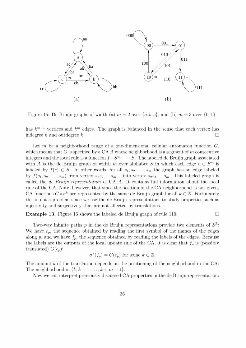
Example 12. Figure 15(a) shows the de Bruijn graph of width m = 2 over three letteralphabet S = a, b, c, while Figure 15(b) shows the de Bruijn graph of width m = 3 overtwo letter alphabet S = 0, 1. In general, the de Bruijn graph of width m over k symbols

35

cc

a

bc

aa

abac ba

bb

bcca

cb111

00 01

1110

000

001

010011

100 101

110

(a) (b)

Figure 15: De Bruijn graphs of width (a) m = 2 over a, b, c, and (b) m = 3 over 0, 1.

has km−1 vertices and km edges. The graph is balanced in the sense that each vertex hasindegree k and outdegree k. ¤

Let m be a neighborhood range of a one-dimensional cellular automaton function G,which means that G is specified by a CA A whose neighborhood is a segment of m consecutiveintegers and the local rule is a function f : Sm −→ S. The labeled de Bruijn graph associatedwith A is the de Bruijn graph of width m over alphabet S in which each edge e ∈ Sm islabeled by f(e) ∈ S. In other words, for all s1, s2, . . . , sm the graph has an edge labeledby f(s1, s2, . . . , sm) from vertex s1s2 . . . sm−1 into vertex s2s3 . . . sm. This labeled graph iscalled the de Bruijn representation of CA A. It contains full information about the localrule of the CA. Note, however, that since the position of the CA neighborhood is not given,CA functions G σk are represented by the same de Bruijn graph for all k ∈ Z. Fortunatelythis is not a problem since we use the de Bruijn representations to study properties such asinjectivity and surjectivity that are not affected by translations.

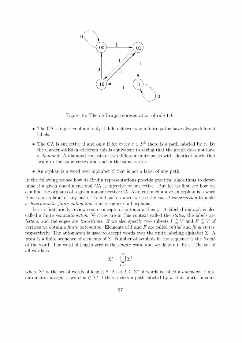
Example 13. Figure 16 shows the labeled de Bruijn graph of rule 110. ¤

Two-way infinite paths p in the de Bruijn representations provide two elements of SZ:We have cp, the sequence obtained by reading the first symbol of the names of the edgesalong p, and we have fp, the sequence obtained by reading the labels of the edges. Becausethe labels are the outputs of the local update rule of the CA, it is clear that fp is (possiblytranslated) G(cp):

σk(fp) = G(cp) for some k ∈ Z.

The amount k of the translation depends on the positioning of the neighborhood in the CA:The neighborhood is k, k + 1, . . . , k + m− 1.

Now we can interpret previously discussed CA properties in the de Bruijn representation:

36

1

00 01

1110

0

0

01

1

1

1

Figure 16: The de Bruijn representation of rule 110.

• The CA is injective if and only if different two-way infinite paths have always differentlabels.

• The CA is surjective if and only if for every c ∈ SZ there is a path labeled by c. Bythe Garden-of-Eden -theorem this is equivalent to saying that the graph does not havea diamond : A diamond consists of two different finite paths with identical labels thatbegin in the same vertex and end in the same vertex.

• An orphan is a word over alphabet S that is not a label of any path.

In the following we see how de Bruijn representations provide practical algorithms to deter-mine if a given one-dimensional CA is injective or surjective. But let us first see how wecan find the orphans of a given non-surjective CA. As mentioned above an orphan is a wordthat is not a label of any path. To find such a word we use the subset construction to makea deterministic finite automaton that recognizes all orphans.

Let us first briefly review some concepts of automata theory. A labeled digraph is alsocalled a finite semiautomaton. Vertices are in this context called the states, the labels areletters, and the edges are transitions. If we also specify two subsets I ⊆ V and F ⊆ V ofvertices we obtain a finite automaton. Elements of I and F are called initial and final states,respectively. The automaton is used to accept words over the finite labeling alphabet Σ. Aword is a finite sequence of elements of Σ. Number of symbols in the sequence is the lengthof the word. The word of length zero is the empty word, and we denote it by ε. The set ofall words is

Σ∗ =∞⋃

k=0

Σk

where Σk is the set of words of length k. A set L ⊆ Σ∗ of words is called a language. Finiteautomaton accepts a word w ∈ Σ∗ if there exists a path labeled by w that starts in some

37

initial state and ends in a final state. The language recognized by a finite automaton is theset of all words that it accepts. Languages that are recognized by finite automata are calledregular. We call two finite automata equivalent if they recognize the same language.

Using the automata theoretic terminology we note that the orphans of a cellular automa-ton are precisely the words that are not accepted by the automaton that we get from the deBruijn graph by making all states initial and final.

A finite automaton is called deterministic if there is only one initial state, and for eachstate v ∈ V and letter a ∈ Σ there is at most one transition with label a from state v. Sincethere is now only one possible continuation from every state with each letter, it is clear thatfor every input word w ∈ Σ∗ there is at most one path that starts in the initial state. Wordw is accepted if and only if the last state of this path is a final state. A deterministic finiteautomaton is complete if there is a (unique) transition from every state with every inputletter. It is easy to make any deterministic finite automaton complete by adding a new state(which is not final) and making all missing transitions into this sink state. Clearly exactlythe same words are accepted as before.

The power set construction is a way to convert an arbitrary finite automaton into anequivalent deterministic and complete automaton. The power set automaton has state set2V , that is, all subsets of V are states. For any X ⊆ V and a ∈ Σ the transition from Xwith input letter a is made into the state

v ∈ V | for some x ∈ X there is an edge x → v with label a .

One easily sees that in the power set automaton the last state of the path that starts atstate X ⊆ V and is labeled by word w consists of all those states v ∈ V such that there is apath from some element of X into v labeled by w in the original automaton. In particular,if we make I the initial state, and make every set X ⊆ V such that X ∩ F 6= ∅ a final stateof the power set automaton, then exactly the same words are accepted that were acceptedin the original automaton. Moreover, if we swap the final states so that we instead make astate X ⊆ V final iff X ∩ F = ∅ then we have a deterministic automaton that accepts thecomplement language.

Let us perform the subset construction on the de Bruijn representation of a CA, where allstates are considered initial and final. We obtain a complete deterministic finite automatonthat accepts the words that are not orphans. Its initial state is Sm−1 and all states except ∅are final. Let’s swap the final states, which means that ∅ becomes the only final state. Thenwe get an automaton that accepts exactly the orphans. We see:

Proposition 25 The set of all orphans of a one-dimensional CA is a regular language. ¤

Note: many states of the power set automaton may be unreachable from the initial state.Such states can be removed from the automaton without affecting the language it recognizes.

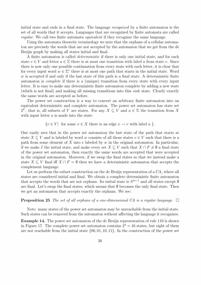
Example 14. The power set automaton of the de Bruijn representation of rule 110 is shownin Figure 17. The complete power set automaton contains 24 = 16 states, but eight of themare not reachable from the initial state 00, 01, 10, 11. In the construction of the power set

38

1

000110 11

0011

0110 00 01

1011

011011

0

0

0

0

0

00

1

1

1

11

1 0,1

Figure 17: A deterministic automaton for the orphans in rule 110. State 00, 01, 10, 11 isthe initial state and state ∅ is the only final state.

automaton it is best to begin from the initial state Sm−1 and add new states as they arereached. In this way only the reachable part ever gets constructed.

The label of the shortest path from the initial state 00, 01, 10, 11 to the final state ∅ is01010. It is hence the shortest orphan of rule 110. The shortest path can always be foundusing the breadth-first search in the graph. We can also make the observation that onlywords containing the pattern 010 can be orphans in rule 110, so any configuration whichdoes not have isolated 1’s has a pre-image. ¤

Let us next move on to the problem of testing a one-dimensional CA function G forinjectivity and surjectivity. Both these questions boil down to the question of which con-figurations have the same image under G. For this we use the following cartesian productconstruction.

From the de Bruijn representation of a CA we form a pair graph whose vertex set isV × V where V = Sm−1 is the vertex set of the de Bruijn representation. In the pair graphthere is an edge (with label a ∈ S) from (u1, u2) ∈ V ×V into (v1, v2) ∈ V ×V if and only ifin the de Bruijn graph there are edges with the same label a from u1 to v1 and from u2 tov2. See Figure 18 for the pair graph of rule 110.

Any two-way infinite path p in the pair graph corresponds to two paths in the original deBruijn automaton, obtained by reading only the first or the second components of the pairs.Both paths have the same edge labels, so they correspond to two configurations of the CAwith the same image. Let us denote these configurations by c1

p and c2p. The correspondence

p ↔ (c1p, c

2p)

is a bijection between paths p and pairs of configurations that satisfy G(c1p) = G(c2

p).Let us denote by

∆ = (u, u) | u ∈ V

39

∆

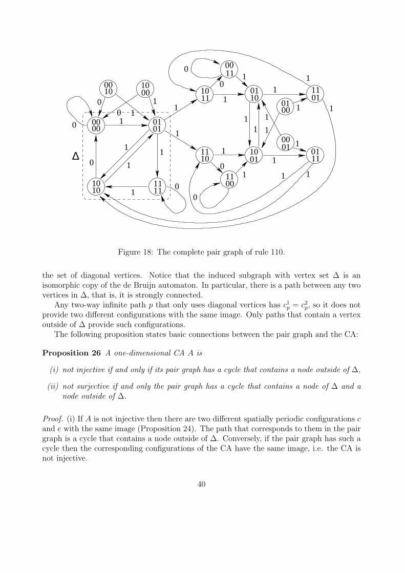
00

00

01

01

01

01

10

10

10

1011

11

11

11

11

11

0100

0100

01

1

1

1

1

0000

0000

0101

1010

1010

1111

0

0

1

1

0

0

1

1

0

0

1

1

1

1

1

1

11

1

1

1

1

00

11

1

1

Figure 18: The complete pair graph of rule 110.

the set of diagonal vertices. Notice that the induced subgraph with vertex set ∆ is anisomorphic copy of the de Bruijn automaton. In particular, there is a path between any twovertices in ∆, that is, it is strongly connected.

Any two-way infinite path p that only uses diagonal vertices has c1p = c2

p, so it does notprovide two different configurations with the same image. Only paths that contain a vertexoutside of ∆ provide such configurations.

The following proposition states basic connections between the pair graph and the CA:

Proposition 26 A one-dimensional CA A is

(i) not injective if and only if its pair graph has a cycle that contains a node outside of ∆,

(ii) not surjective if and only the pair graph has a cycle that contains a node of ∆ and anode outside of ∆.

Proof. (i) If A is not injective then there are two different spatially periodic configurations cand e with the same image (Proposition 24). The path that corresponds to them in the pairgraph is a cycle that contains a node outside of ∆. Conversely, if the pair graph has such acycle then the corresponding configurations of the CA have the same image, i.e. the CA isnot injective.

40

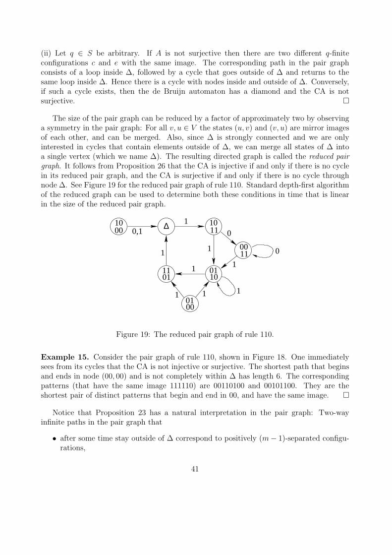
(ii) Let q ∈ S be arbitrary. If A is not surjective then there are two different q-finiteconfigurations c and e with the same image. The corresponding path in the pair graphconsists of a loop inside ∆, followed by a cycle that goes outside of ∆ and returns to thesame loop inside ∆. Hence there is a cycle with nodes inside and outside of ∆. Conversely,if such a cycle exists, then the de Bruijn automaton has a diamond and the CA is notsurjective. ¤

The size of the pair graph can be reduced by a factor of approximately two by observinga symmetry in the pair graph: For all v, u ∈ V the states (u, v) and (v, u) are mirror imagesof each other, and can be merged. Also, since ∆ is strongly connected and we are onlyinterested in cycles that contain elements outside of ∆, we can merge all states of ∆ intoa single vertex (which we name ∆). The resulting directed graph is called the reduced pairgraph. It follows from Proposition 26 that the CA is injective if and only if there is no cyclein its reduced pair graph, and the CA is surjective if and only if there is no cycle throughnode ∆. See Figure 19 for the reduced pair graph of rule 110. Standard depth-first algorithmof the reduced graph can be used to determine both these conditions in time that is linearin the size of the reduced pair graph.

∆1000

1011

0011

0110

1101

0100

0,11

1

1

11

111

0

0

Figure 19: The reduced pair graph of rule 110.

Example 15. Consider the pair graph of rule 110, shown in Figure 18. One immediatelysees from its cycles that the CA is not injective or surjective. The shortest path that beginsand ends in node (00, 00) and is not completely within ∆ has length 6. The correspondingpatterns (that have the same image 111110) are 00110100 and 00101100. They are theshortest pair of distinct patterns that begin and end in 00, and have the same image. ¤

Notice that Proposition 23 has a natural interpretation in the pair graph: Two-wayinfinite paths in the pair graph that

• after some time stay outside of ∆ correspond to positively (m− 1)-separated configu-rations,

41

• before some time stay outside of ∆ correspond to negatively (m− 1)-separated config-urations, and

• always stay outside of ∆ correspond to totally (m− 1)-separated configurations

with the same image under G.

2.7 Two-dimensional CA and tilings

Proposition 7 and Corollaries 17, 10 and 19 prove all positive implications in Figure 9. Forthe negative implications that are common with the one-dimensional case we use the one-dimensional CA of Example 11. The d-dimensional version of this CA uses neighborhood(0, 0, . . . , 0), (1, 0, 0, . . . , 0) and the same local rule f . This means that the space consistsof independently operating one-dimensional CA along the first dimension. It was shown inExample 11 that the one-dimensional version is surjective but not injective. The restrictionGF to finite configurations is surjective if 2 is taken as the quiescent state and not surjectiveif 0 is taken as the quiescent state. In the one-dimensional case injectivity and surjectivity ofG are always equivalent to the injectivity and surjectivity, respectively, of GP , the restrictionof G to totally periodic configurations, so GP in this example is surjective but not injective.Clearly the d-dimensional version has all these same properties, so this example provides allthe negative implications shown in Figure 9 except for one. To complete the picture we needan example of a two-dimensional CA which is not reversible, while GP is injective. For suchan example, and for other forthcoming considerations on two-dimensional CA, we turn toplane tilings.

Tilings are a topic of another course Tilings and Patterns, so we refer to that class formore details and complete proofs of the results concerning tilings. However, we can easilypresent here the relevant results (without proofs), and see how they can be applied on cellularautomata.

A tile set T = (T, N,R) consists of a finite set T whose elements are the tiles, a neigh-borhood vector N defined analogously to (1) as a vector of m distinct elements of Z2, anda local matching rule R ⊆ Tm which gives a relation specifying which tilings are consideredvalid. Tilings are configurations t ∈ T Z

2. A tiling is valid at cell ~n ∈ Z2 if and only if

[t(~n + ~n1), t(~n + ~n2), . . . , t(~n + ~nm)] ∈ R,

that is, the neighborhood of ~n contains a matching combination of tiles. Tiling t ∈ T Z2

iscalled valid if it is valid at all positions ~n ∈ Z2, and we say that the tile set T then admitstiling t. Let V (T ) be the set of all valid tilings admitted by T .

There is an apparent similarity in the definitions of tile sets and two-dimensional cellularautomata. The only difference is that instead of a dynamic local rule f , tilings are basedon a static matching relation R. In symbolic dynamics terminology, the fact that V (T ) isdefined by forbidding a finite collection of patterns means that V (T ) is a two-dimensionalsubshift of finite type.

42

A fundamental property of cellular automata is that they commute with translations.The tiling counter part states the obvious fact that set V (T ) is invariant under translations.The second fundamental property is the continuity of CA functions. A tiling counter partof this fact states that the set of valid tilings is closed, that is, the limit of a convergingsequence of valid tilings is also valid. Proofs are straightforward.

Proposition 27 Let T = (T, N, R) be a tile set.

(i) If t is a valid tiling and τ is a translation of the plane then τ t is a valid tiling.

(ii) Suppose t1, t2, . . . is a converging sequence where for every ~n ∈ Z2 there is k such thatti is valid at cell ~n for all i ≥ k. Then limi→∞ ti is a valid tiling.

¤A direct consequence of (ii) is that a tile set that can tile arbitrarily large squares, admits

a tiling of the whole space:

Corollary 28 Suppose T = (T, N, R) is a tile set such that for every finite D ⊆ Z2 there ist ∈ T Z

2that is valid at every ~n ∈ D. Then T admits a valid tiling of the plane.

Proof. Let ~r1, ~r2, . . . be an enumeration of elements of Z2, and for every j ∈ Z+ let

Dj = ~r1, ~r2, . . . , ~rj.The hypothesis of the corollary states that there is tj ∈ T Z

2that is valid at every ~n ∈ Dj.

Let t be the limit of a converging subsequence of t1, t2, . . .. It follows from Proposition 27(ii)that t is a valid tiling. ¤

A popular way to describe a tile set is to use Wang tiles. Wang tiles use the von Neumannneighborhood. The tiles are viewed as unit squares whose edges are colored, and the localmatching rule is given in terms of these colors: A tiling is valid at cell ~n ∈ Z2 iff each of thefour edges of the tile in position ~n have the same color as the abutting edge in the adjacenttile.

Example 16. Consider the two Wang-tiles A and B shown in Figure 20(a). Since all fourneighbors of tile A have to be copies of B, and vice versa, the only valid tilings are infinitecheckerboards where A’s and B’s alternate, as shown in Figure 20(b). ¤

Let ~r 6= ~0. A tiling t ∈ T Z2

is called ~r-periodic if it is invariant under translation by ~r,that is, if

t(~n) = t(~n + ~r) for all ~n ∈ Zd.

A tiling is totally periodic if it is periodic with respect to two linearly independent vectors.A totally periodic tiling is always periodic with respect to σk

1 and σk2 for some k > 0, where

σ1 and σ2 are the horizontal and vertical shifts by one cell. The tiling in Figure 20(b) istotally periodic since it is invariant under σ2

1 and σ22.

The following proposition states the fact that if a tile set admits some periodic tilingthen it also admits a totally periodic tiling:

43

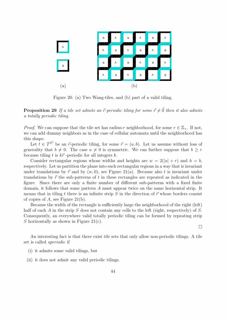
B

A

(a)

A

B

A

AB

A B

B

A B A B

A B A B

A

B A B A

BAB

(b)

Figure 20: (a) Two Wang-tiles, and (b) part of a valid tiling.

Proposition 29 If a tile set admits an ~r-periodic tiling for some ~r 6= ~0 then it also admitsa totally periodic tiling.

Proof. We can suppose that the tile set has radius-r neighborhood, for some r ∈ Z+. If not,we can add dummy neighbors as in the case of cellular automata until the neighborhood hasthis shape.

Let t ∈ T Z2

be an ~r-periodic tiling, for some ~r = (a, b). Let us assume without loss ofgenerality that b 6= 0. The case a 6= 0 is symmetric. We can further suppose that b ≥ rbecause tiling t is k~r -periodic for all integers k.

Consider rectangular regions whose widths and heights are w = 2(|a| + r) and h = b,respectively. Let us partition the plane into such rectangular regions in a way that is invariantunder translations by ~r and by (w, 0), see Figure 21(a). Because also t is invariant undertranslations by ~r the sub-patterns of t in these rectangles are repeated as indicated in thefigure. Since there are only a finite number of different sub-patterns with a fixed finitedomain, it follows that some pattern A must appear twice on the same horizontal strip. Itmeans that in tiling t there is an infinite strip S in the direction of ~r whose borders consistof copies of A, see Figure 21(b).

Because the width of the rectangle is sufficiently large the neighborhood of the right (left)half of each A in the strip S does not contain any cells to the left (right, respectively) of S.Consequently, an everywhere valid totally periodic tiling can be formed by repeating stripS horizontally as shown in Figure 21(c).

¤

An interesting fact is that there exist tile sets that only allow non-periodic tilings. A tileset is called aperiodic if

(i) it admits some valid tilings, but

(ii) it does not admit any valid periodic tilings.

44

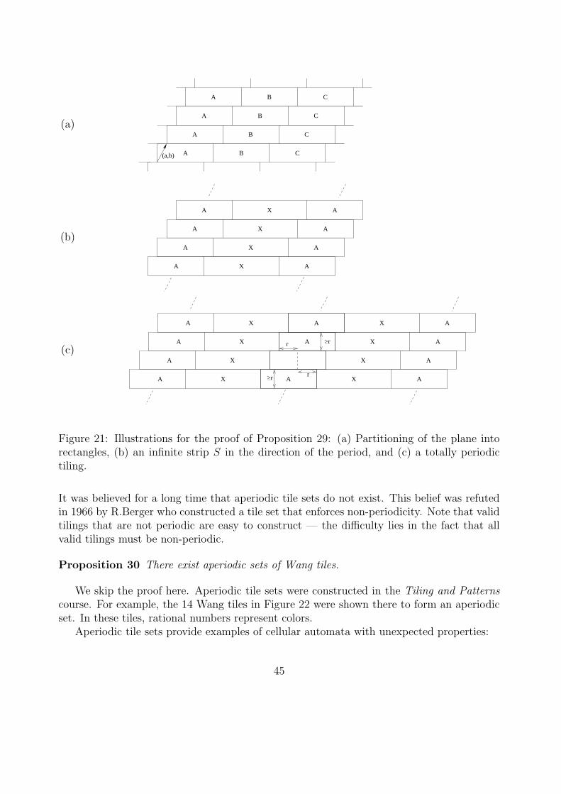
(a,b) A B C

A B C

A B C

A B C

(a)

A X A

A X A

A X A

A X A

(b)

A

r

r

>r

>r

X

X

X

X X

X

X

XA

A

A

A A

A

A A

A

A

(c)

Figure 21: Illustrations for the proof of Proposition 29: (a) Partitioning of the plane intorectangles, (b) an infinite strip S in the direction of the period, and (c) a totally periodictiling.

It was believed for a long time that aperiodic tile sets do not exist. This belief was refutedin 1966 by R.Berger who constructed a tile set that enforces non-periodicity. Note that validtilings that are not periodic are easy to construct — the difficulty lies in the fact that allvalid tilings must be non-periodic.

Proposition 30 There exist aperiodic sets of Wang tiles.

We skip the proof here. Aperiodic tile sets were constructed in the Tiling and Patternscourse. For example, the 14 Wang tiles in Figure 22 were shown there to form an aperiodicset. In these tiles, rational numbers represent colors.

Aperiodic tile sets provide examples of cellular automata with unexpected properties:

45

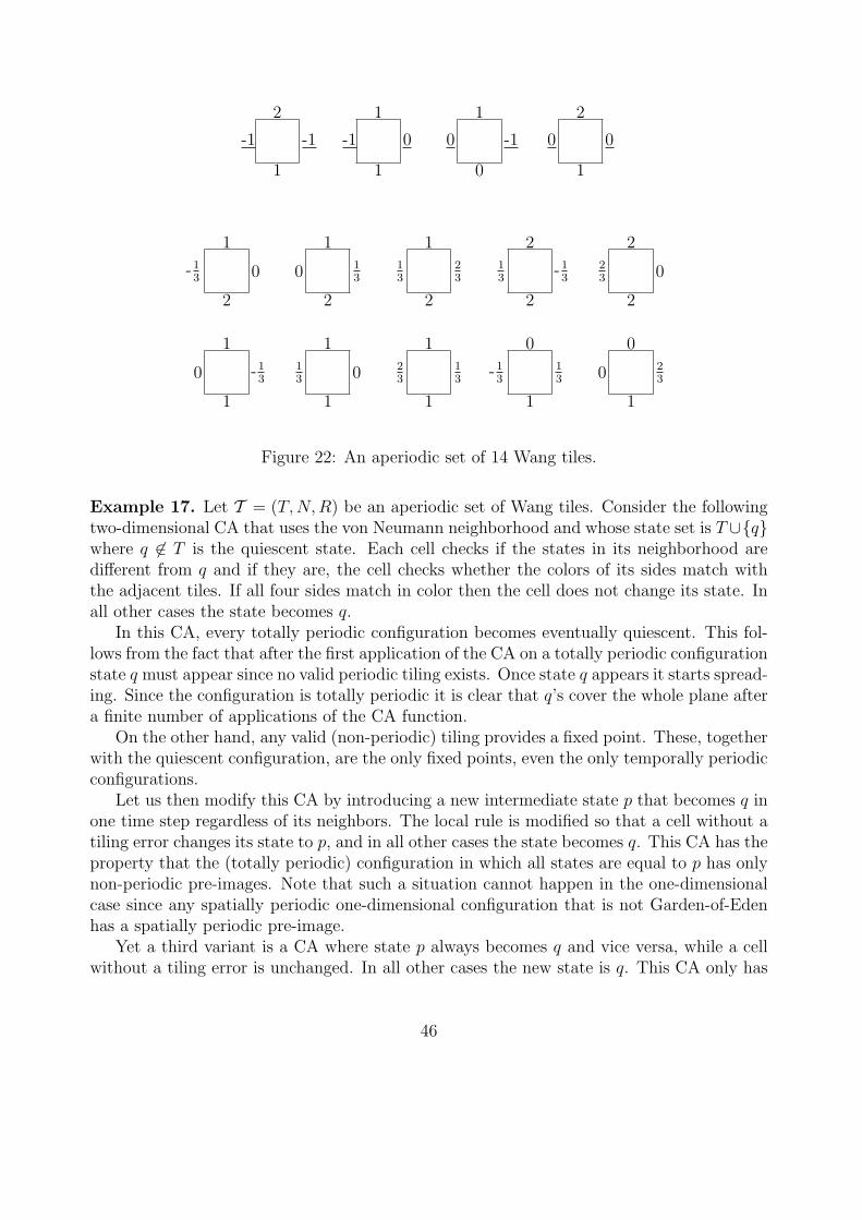
1

-1 -1

2

1

-1 0

1

0

0 -1

1

1

0 0

2

2

-13 0

1

2

0 13

1

2

13

23

1

2

13

-13

2

2

23 0

2

1

0 -13

1

1

13 0

1

1

23

13

1

1

-13

13

0

1

0 23

0

Figure 22: An aperiodic set of 14 Wang tiles.

Example 17. Let T = (T, N, R) be an aperiodic set of Wang tiles. Consider the followingtwo-dimensional CA that uses the von Neumann neighborhood and whose state set is T ∪qwhere q 6∈ T is the quiescent state. Each cell checks if the states in its neighborhood aredifferent from q and if they are, the cell checks whether the colors of its sides match withthe adjacent tiles. If all four sides match in color then the cell does not change its state. Inall other cases the state becomes q.

In this CA, every totally periodic configuration becomes eventually quiescent. This fol-lows from the fact that after the first application of the CA on a totally periodic configurationstate q must appear since no valid periodic tiling exists. Once state q appears it starts spread-ing. Since the configuration is totally periodic it is clear that q’s cover the whole plane aftera finite number of applications of the CA function.

On the other hand, any valid (non-periodic) tiling provides a fixed point. These, togetherwith the quiescent configuration, are the only fixed points, even the only temporally periodicconfigurations.

Let us then modify this CA by introducing a new intermediate state p that becomes q inone time step regardless of its neighbors. The local rule is modified so that a cell without atiling error changes its state to p, and in all other cases the state becomes q. This CA has theproperty that the (totally periodic) configuration in which all states are equal to p has onlynon-periodic pre-images. Note that such a situation cannot happen in the one-dimensionalcase since any spatially periodic one-dimensional configuration that is not Garden-of-Edenhas a spatially periodic pre-image.

Yet a third variant is a CA where state p always becomes q and vice versa, while a cellwithout a tiling error is unchanged. In all other cases the new state is q. This CA only has

46

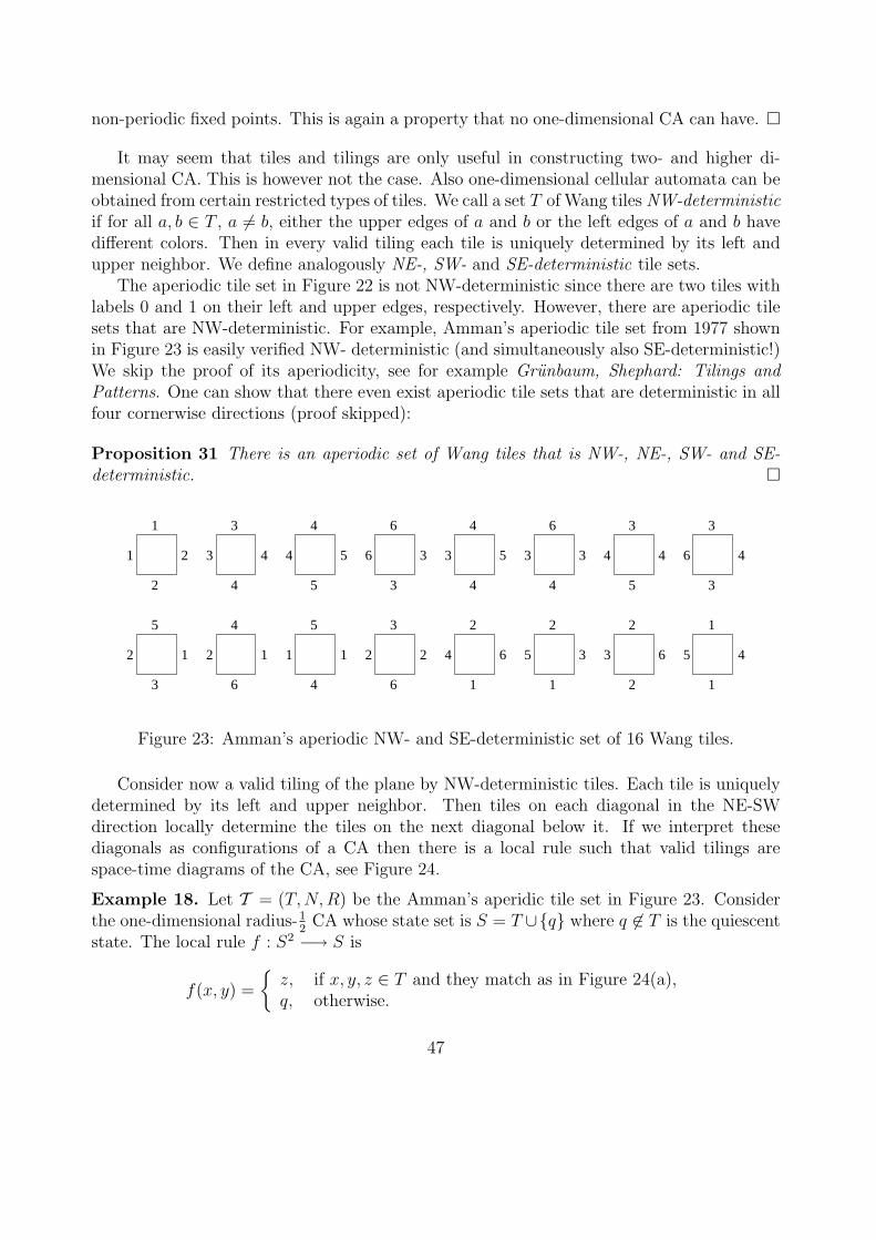
non-periodic fixed points. This is again a property that no one-dimensional CA can have. ¤

It may seem that tiles and tilings are only useful in constructing two- and higher di-mensional CA. This is however not the case. Also one-dimensional cellular automata can beobtained from certain restricted types of tiles. We call a set T of Wang tiles NW-deterministicif for all a, b ∈ T , a 6= b, either the upper edges of a and b or the left edges of a and b havedifferent colors. Then in every valid tiling each tile is uniquely determined by its left andupper neighbor. We define analogously NE-, SW- and SE-deterministic tile sets.

The aperiodic tile set in Figure 22 is not NW-deterministic since there are two tiles withlabels 0 and 1 on their left and upper edges, respectively. However, there are aperiodic tilesets that are NW-deterministic. For example, Amman’s aperiodic tile set from 1977 shownin Figure 23 is easily verified NW- deterministic (and simultaneously also SE-deterministic!)We skip the proof of its aperiodicity, see for example Grunbaum, Shephard: Tilings andPatterns. One can show that there even exist aperiodic tile sets that are deterministic in allfour cornerwise directions (proof skipped):

Proposition 31 There is an aperiodic set of Wang tiles that is NW-, NE-, SW- and SE-deterministic. ¤

4

2

1

1

2

3 4

3

4

4

4 6

6

5

5

3

3

2

5

2

4 5

1 2

3

3

1 1

6 4

1

6

2

3

4

3

6

4

3

6

3

4

5

4

3

5

4

3

4

4

2

5

2

3

2

5

1

1

6

1

3

2

6

1

Figure 23: Amman’s aperiodic NW- and SE-deterministic set of 16 Wang tiles.

Consider now a valid tiling of the plane by NW-deterministic tiles. Each tile is uniquelydetermined by its left and upper neighbor. Then tiles on each diagonal in the NE-SWdirection locally determine the tiles on the next diagonal below it. If we interpret thesediagonals as configurations of a CA then there is a local rule such that valid tilings arespace-time diagrams of the CA, see Figure 24.

Example 18. Let T = (T, N, R) be the Amman’s aperidic tile set in Figure 23. Considerthe one-dimensional radius-1

2CA whose state set is S = T ∪q where q 6∈ T is the quiescent

state. The local rule f : S2 −→ S is

f(x, y) =

z, if x, y, z ∈ T and they match as in Figure 24(a),q, otherwise.

47

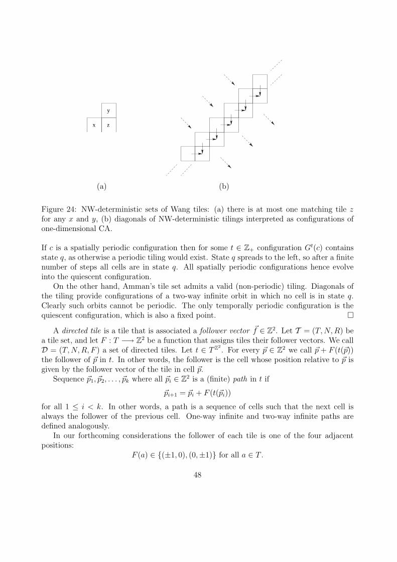
x

y

z

(a) (b)

Figure 24: NW-deterministic sets of Wang tiles: (a) there is at most one matching tile zfor any x and y, (b) diagonals of NW-deterministic tilings interpreted as configurations ofone-dimensional CA.

If c is a spatially periodic configuration then for some t ∈ Z+ configuration Gt(c) containsstate q, as otherwise a periodic tiling would exist. State q spreads to the left, so after a finitenumber of steps all cells are in state q. All spatially periodic configurations hence evolveinto the quiescent configuration.

On the other hand, Amman’s tile set admits a valid (non-periodic) tiling. Diagonals ofthe tiling provide configurations of a two-way infinite orbit in which no cell is in state q.Clearly such orbits cannot be periodic. The only temporally periodic configuration is thequiescent configuration, which is also a fixed point. ¤

A directed tile is a tile that is associated a follower vector ~f ∈ Z2. Let T = (T, N, R) bea tile set, and let F : T −→ Z2 be a function that assigns tiles their follower vectors. We callD = (T,N,R, F ) a set of directed tiles. Let t ∈ T Z

2. For every ~p ∈ Z2 we call ~p + F (t(~p))

the follower of ~p in t. In other words, the follower is the cell whose position relative to ~p isgiven by the follower vector of the tile in cell ~p.

Sequence ~p1, ~p2, . . . , ~pk where all ~pi ∈ Z2 is a (finite) path in t if

~pi+1 = ~pi + F (t(~pi))

for all 1 ≤ i < k. In other words, a path is a sequence of cells such that the next cell isalways the follower of the previous cell. One-way infinite and two-way infinite paths aredefined analogously.

In our forthcoming considerations the follower of each tile is one of the four adjacentpositions:

F (a) ∈ (±1, 0), (0,±1) for all a ∈ T .

48

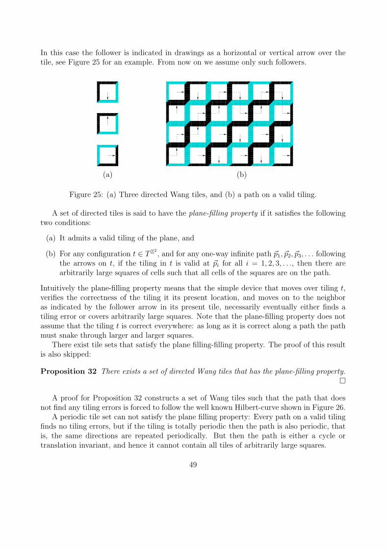
In this case the follower is indicated in drawings as a horizontal or vertical arrow over thetile, see Figure 25 for an example. From now on we assume only such followers.

(a)

(b)

Figure 25: (a) Three directed Wang tiles, and (b) a path on a valid tiling.

A set of directed tiles is said to have the plane-filling property if it satisfies the followingtwo conditions:

(a) It admits a valid tiling of the plane, and

(b) For any configuration t ∈ T Z2, and for any one-way infinite path ~p1, ~p2, ~p3, . . . following

the arrows on t, if the tiling in t is valid at ~pi for all i = 1, 2, 3, . . ., then there arearbitrarily large squares of cells such that all cells of the squares are on the path.

Intuitively the plane-filling property means that the simple device that moves over tiling t,verifies the correctness of the tiling it its present location, and moves on to the neighboras indicated by the follower arrow in its present tile, necessarily eventually either finds atiling error or covers arbitrarily large squares. Note that the plane-filling property does notassume that the tiling t is correct everywhere: as long as it is correct along a path the pathmust snake through larger and larger squares.

There exist tile sets that satisfy the plane filling-filling property. The proof of this resultis also skipped:

Proposition 32 There exists a set of directed Wang tiles that has the plane-filling property.¤

A proof for Proposition 32 constructs a set of Wang tiles such that the path that doesnot find any tiling errors is forced to follow the well known Hilbert-curve shown in Figure 26.

A periodic tile set can not satisfy the plane filling property: Every path on a valid tilingfinds no tiling errors, but if the tiling is totally periodic then the path is also periodic, thatis, the same directions are repeated periodically. But then the path is either a cycle ortranslation invariant, and hence it cannot contain all tiles of arbitrarily large squares.

49

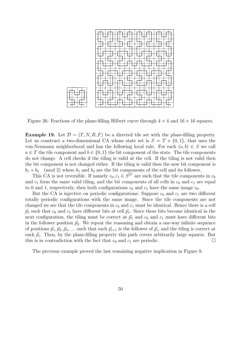
Figure 26: Fractions of the plane-filling Hilbert curve through 4× 4 and 16× 16 squares.

Example 19. Let D = (T, N, R, F ) be a directed tile set with the plane-filling property.Let us construct a two-dimensional CA whose state set is S = T × 0, 1, that uses thevon-Neumann neighborhood and has the following local rule. For each (a, b) ∈ S we calla ∈ T the tile component and b ∈ 0, 1 the bit component of the state. The tile componentsdo not change. A cell checks if the tiling is valid at the cell. If the tiling is not valid thenthe bit component is not changed either. If the tiling is valid then the new bit component isb1 + b2 (mod 2) where b1 and b2 are the bit components of the cell and its follower.

This CA is not reversible. If namely c0, c1 ∈ SZ2

are such that the tile components in c0

and c1 form the same valid tiling, and the bit components of all cells in c0 and c1 are equalto 0 and 1, respectively, then both configurations c0 and c1 have the same image c0.

But the CA is injective on periodic configurations: Suppose c0 and c1 are two differenttotally periodic configurations with the same image. Since the tile components are notchanged we see that the tile components in c0 and c1 must be identical. Hence there is a cell~p1 such that c0 and c1 have different bits at cell ~p1. Since these bits become identical in thenext configuration, the tiling must be correct at ~p1 and c0 and c1 must have different bitsin the follower position ~p2. We repeat the reasoning and obtain a one-way infinite sequenceof positions ~p1, ~p2, ~p3, . . . such that each ~pi+1 is the follower of ~pi, and the tiling is correct ateach ~pi. Then, by the plane-filling property this path covers arbitrarily large squares. Butthis is in contradiction with the fact that c0 and c1 are periodic. ¤

The previous example proved the last remaining negative implication in Figure 9.

50

3 Algorithmic aspects

Next we turn to algorithmic aspects of cellular automata. These are two-fold: On one side,there are questions concerning cellular automata (e.g. is a given CA reversible? surjec-tive?) that we want to find algorithms for. It turns out that many of these questions areundecidable, that is, no algorithm exists. On the other hand, cellular automata themselvesare computation devices that can be used to solve algorithmic questions. We investigatecomputational universality in cellular automata.

First we review some basic concepts of the theory of computability.

3.1 Algorithms, semi-algorithms and undecidability

Intuitively, an algorithm is a mechanical procedure, specified by a finite set of instructions, tosolve some well-defined computational problem. The problem has an input instance, and thealgorithm, after a finite number of processing steps, must return the answer to the problemfor the given instance. We focus on algorithms for decision problems. These are problemswhere the answer for each instance is either ”yes” or ”no”. For example, the questionwhether a given cellular automaton is reversible is a decision problem. An instance of thisproblem is a cellular automaton, and the answer is ”yes” or ”no” depending on whether theCA is reversible or not. We will call these positive and negative instances of the problem,respectively.

Computer programming is common place. There is widespread acceptance that algo-rithms are processes that can be implemented as programs in some standard programminglanguage, say for example, in C. So in the following discussion algorithms for decision prob-lems will be understood as computer programs that take the instance of the problem asinput, and return answer ”yes” or ”no”. Rather than providing actual syntactically cor-rect programs, algorithms will be described in plain English in sufficient details so that anexperienced programmer easily can implement the algorithm on a computer.

A semi-algorithm for a decision problem is an algorithm like process that correctly returnsvalue ”yes” for positive instances, but on negative instances the semi-algorithm does notreturn any value, i.e. it runs for ever without ever halting. Since ”yes” is the only possibleoutput from a semi-algorithm we can simply state that the input instance is positive if andonly if the semi-algorithm halts. Notice that there is non-symmetry between the positive andnegative instances. So a semi-algorithm for reversibility of cellular automata is not a semi-algorithm for non-reversibility. The decision problem obtained by swapping the negative andpositive instances is called the complement of the original problem.

If an algorithm exists for a decision problem then we say that the decision problem isdecidable. Otherwise it is undecidable. If a semi-algorithm exists then the problem is calledsemi-decidable. Note the following obvious facts:

(i) If a problem is decidable then also the complement problem is decidable.

(ii) Every decidable problem is also semi-decidable.

51

(iii) If a problem and its complement are both semi-decidable then the problem is decidable.

For observation (iii) note that the two semi-algorithms for the problem and its complementcan be executed concurrently until one of them returns the answer.

Example 20. The decision problem

1D ReversibilityInstance: One-dimensional cellular automaton AProblem: Is A reversible ?

is decidable. An algorithm based on the pair graph was described in Section 2.6. Also theproblem

1D SurjectivityInstance: One-dimensional cellular automaton AProblem: Is A surjective ?

was shown decidable by the pair graphs technique. The higher dimensional variants are morecomplicated.

2D ReversibilityInstance: Two-dimensional cellular automaton AProblem: Is A reversible ?

is semi-decidable: A semi-algorithm enumerates one-by-one all two-dimensional cellular au-tomata X that have the same state set as A, and tests for each candidate whether X Acomputes the identity function. If such an X is found then the semi-algorithm halts, indi-cating that the input A is reversible, otherwise the process continues without ever halting.Observe that one can effectively construct candidates X one-by-one, form the compositionX A and test for equivalence with the identity function.

Later we see that 2D Reversibility is undecidable, so no semi-algorithm exists for recog-nizing non-reversible CA. The decision problem

2D SurjectivityInstance: Two-dimensional cellular automaton AProblem: Is A surjective ?

is not semi-decidable, but its complement is. A semi-algorithm for negative instances isbased on looking for an orphan: it enumerates all finite patterns p and checks for each pwhether it is an orphan or not. If an orphan is found then the process halts, indicating thatthe instance is not a surjective CA. On surjective CA the search for an orphan continueswithout ever halting. ¤

In practice, the input to a program is an encoding of an instance as a string. This isclear in the programming context, since the input to the program will be keyed in froma keyboard, or read in from a file. In any case, inside the computer, the input will berepresented as a sequence of bits, that is, as a word over the two letter alphabet 0, 1.

52

Each decision problem can now be associated a language over the encoding alphabet: thelanguage contains all those words that are encodings of positive instances. Then solving thedecision problem is equivalent to determining if a given word belongs to the correspondinglanguage. Notice that there are actually three types of words: encodings of positive instances,encodings of negative instances and those words that are not valid encodings of any instances.In the following we always assume that the encoding is effective in the sense that there is analgorithm to determine if a given word is a valid encoding. Also the way the instances areencoded should be natural so that the decision problem is not solved or otherwise affectedby the encoding. (For example adding letter ”+” or ”-” in front of the word to indicatewhether it is an encoding of a positive or negative instance is not acceptable, since then thedecision problem must be solved already during the encoding process!) Actually all resultsconcerning the decidability of a decision problem are relative to the encoding used, but allreasonable encodings are equivalent with each other in the sense that there are algorithms toconvert between the encodings, which means that the decidability/semi-decidability statusis unaffected by the choice of the encoding.

The decision problem whether a given word belongs to language L ⊆ Σ∗ is called themembership problem of language L. Language L is called recursive if its membership problemis decidable, and it is called recursively enumerable (or r.e. for short) if its membershipproblem is semi-decidable. Clearly a decision problem is decidable (or semi-decidable) if andonly if the membership problem for the corresponding language is recursive (or recursivelyenumerable, respectively).

The number of different algorithms and semi-algorithms is countable. Each algorithm cannamely be represented as a finite string (e.g. its source code in programming language C),and the number of different strings over any alphabet is countable. This means that there areonly countably many recursive and recursively enumerable languages over any alphabet Σ.On the other hand, there are uncountably many different languages L ⊆ Σ∗, which impliesthat many languages are not recursive (or even recursively enumerable). Their membershipproblem is not decidable (or semi-decidable), so we see that there are many undecidabledecision problems. This is not surprising, but what is more interesting is that we can provesome individual problems undecidable, and that many of these undecidable problems arequite natural and appear in many contexts.

To obtain our first undecidable decision problem we turn to (semi-)algorithms whoseinput is a semi-algorithm A. This of course means that the input is an encoding of A as, say,a binary string representing the source code for A in language C. To clarify the distinctionwe’ll denote by 〈A〉 the encoding of A over the binary alphabet. An algorithm call to A withinput w will be denoted by A(w).

The decision problem that we first prove undecidable is the following:

Semi-algorithm haltingInstance: A semi-algorithm 〈A〉 and an input string w ∈ Σ∗

Problem: Does A halt on input w ?

Proposition 33 The decision problem Semi-algorithm halting is undecidable.

53

Proof. Suppose the contrary: There is an algorithm Halt that solves problem Semi-algorithmhalting. In other words, for any binary strings 〈A〉 and w algorithm call Halt(〈A〉, w) returnsvalue ”yes” if A is a semi-algorithm that halts on input w, and Halt(〈A〉, w) returns value”no” otherwise. Using Halt we can construct the following semi-algorithm:

Diag(〈A〉):if Halt(〈A〉, 〈A〉) returns ’’no’’ then halt otherwise loop forever

The semi-algorithm Diag takes as input a binary string 〈A〉. Using an algorithm call toHalt it determines whether the input is the encoding of a semi-algorithm A that halts withinput 〈A〉, i.e. on its own encoding. If Halt(〈A〉, 〈A〉) returns value ”no” then Diag(〈A〉)halts and if Halt(〈A〉, 〈A〉) returns ”yes” then Diag(〈A〉) enters an infinite loop and neverhalts.

Consider the algorithm call Halt(〈Diag〉, 〈Diag〉). If it returns ”yes” then Diag(〈Diag〉)should halt. But following the definition of Diag this means that Halt(〈Diag〉, 〈Diag〉)returned ”no” when Diag made that call, a contradiction.

On the other hand, if Halt(〈Diag〉, 〈Diag〉) returns ”no” then Diag(〈Diag〉) should nothalt. That happens if and only if Halt(〈Diag〉, 〈Diag〉) returns ”yes”, again a contradiction.Both cases lead to a contradiction, so algorithm Halt does not exist. ¤

Note that Semi-algorithm halting is semi-decidable, so its complement problem is not. Tosee the semi-decidability consider the semi-algorithm that on inputs 〈A〉 and w starts tosimulate A on input w step-by-step. Halting of this process correctly identifies the positiveinstances of Semi-algorithm halting.

The proof of Proposition 33 (due to A.Turing) can be understood as a variant of thediagonal argument that Cantor used to prove that certain sets are uncountable. Imaginean infinite two-dimensional matrix M whose rows and columns are indexed by 〈A〉 for allsemi-algorithms A, and where

M [〈A〉, 〈B〉] =

0, if A does not halt on input 〈B〉,1, if A halts on input 〈B〉.

Consider the diagonal elements M [〈A〉, 〈A〉] of the matrix. Reading the diagonal and swap-ping each value 0 ↔ 1 creates a sequence that is different from every row of the matrix.This means that there is no semi-algorithm enlisted that would halt on exactly those inputs〈A〉 for which A does not halt on input 〈A〉. But such a semi-algorithm should exist ifSemi-algorithm halting is decidable.

Once we established the undecidability of Semi-algorithm halting we can use reductionsto obtain new undecidable problems.

Example 21. Let us prove that is undecidable whether a given semi-algorithm halts onsome input.

Sometimes haltingInstance: A semi-algorithm 〈A〉Problem: Does A halt on some input w ?

54

Suppose there is an algorithm S that solves Sometimes halting. Let us describe an algorithmHalt that then solves Semi-algorithm halting: Let 〈A〉 and w be arbitrary inputs to Halt.First string 〈B〉 is created where B is a semi-algorithm that takes one input and works asfollows: B checks whether its input is equal to w. If it is not then it enters an infinite loop.If the input is w then it starts A with input w. Clearly B halts with input w if A halts withinput w and it does not halt on any input if A does not halt on input w.

Note that this B can be effectively created for any given A and w, that is, there is analgorithm that outputs 〈B〉 when it gets 〈A〉 and w as input.

Algorithm Halt next takes 〈B〉 that it created and gives it as input to the hypotheticalalgorithm S. From the answer it can conclude whether A halts on w.

We have described algorithm Halt that solves problem Semi-algorithm halting. This isin contraction to Proposition 33, which means that the hypothetical algorithm S does notexist. ¤

The previous example illustrates the idea of Turing reductions : If we want to prove thatdecision problem P is undecidable we describe an algorithm for some known undecidableproblem U that makes (possibly several) calls to a hypothetical algorithm for P . Since U ispreviously known to be undecidable such algorithm cannot exist. Therefore the hypotheticalalgorithm for P cannot exist either.

Example 21 shows actually a reduction of more restricted type: A many-one reduction isan algorithm that modifies an arbitrary input u for a known undecidable problem U into anequivalent instance p of decision problem P . By equivalent it is meant that p is a positiveinstance of P if and only if u is a positive instance of U . The existence of such reductionsshows that P is undecidable, because otherwise the reduction and an algorithm for P wouldsolve U . Notice that many-one reductions are special types of Turing reductions where thecall to the hypothetical algorithm for P is done only once, as the last step.

Finally, reductions can be used also to show that some decision problem P is not evensemi-decidable. In this case one starts with a hypothetical semi-algorithm S for for P , andshows that there is then a semi-algorithm for some problem U that is previously known notto be semi-decidable. In case of Turing reductions this semi-algorithm is allowed to makeany number of calls to S, while in many-one reductions only one call is made at the end.

3.2 Turing machines

Turing machines are stripped down toy computers that are extremely simple in their defi-nition and step-by-step operations, but nevertheless powerful enough to simulate arbitraryalgorithms. It is actually common to take them as the formal definition of an algorithm.(In this course a different approach was taken and we rather defined algorithms in terms ofcomputer programs, since for most people it is easier to accept these as the proper model ofcomputation.)

There are two reasons for us to introduce Turing machines at this stage:

55

(i) We use reductions to establish new undecidability results. Direct reductions from de-cision problems involving semi-algorithms into simple questions concerning tilings andcellular automata are very laborious as they involve converting given semi-algorithmsinto corresponding tile sets or CA. Reductions from simple devices such as Turingmachines are shorter and easier. So a good approach is to first prove one questionconcerning Turing machines (the halting problem of Turing machines) undecidable,and to make further reduction from this simple set-up.

(ii) We want to show that cellular automata can perform arbitrary computations. Thisrequires simulating arbitrary (semi-)algorithms on cellular automata. As in (i), it ismuch easier to show how to simulate a simple device such as a Turing machine ratherthan an algorithm given in terms of, say, a C-program.

A deterministic Turing machine is specified by the following items:

• A finite state set Q,

• initial, accepting and rejecting states q0, qa, qr ∈ Q, respectively, where qa and qr areboth called halting states and qa 6= qr,

• a finite tape alphabet Γ,

• an input alphabet Σ ⊂ Γ,

• a blank tape symbol b ∈ Γ \ Σ, and

• a transition function δ : Q × Γ −→ Q × Γ × −1, 1. For all γ ∈ Γ we must haveδ(qa, γ) = (qa, γ, 1) and δ(qr, γ) = (qr, γ, 1).

The machine consists of a tape and a control unit. The tape is a two-way infinite sequenceof cells, each capable of storing a letter from the tape alphabet Γ. The tape positions areindexed by Z. The content of the tape at any given time is described by a function t ∈ ΓZ

where t(i) ∈ Γ is the symbol in cell i, for any i ∈ Z.The control unit is a finite state automaton that moves on the tape and is able to read

the symbol at its present location on the tape. Triplets

(q, i, t) ∈ Q× Z× ΓZ

are instantaneous descriptions or the configurations of the Turing machine. They contain allinformation about the present state of the machine: its state q, location i on the tape andthe content t of the tape. Configurations (q, i, t) where q = qa or q = qr are called acceptingand rejecting, respectively. In both cases we say that the Turing machine halts.

In one time step the Turing machine – depending on the state of the control unit andthe tape symbol in the cell it reads – changes the state, replaces the tape symbol by a newone and moves one position to the left or right on the tape, as specified by the transition

56

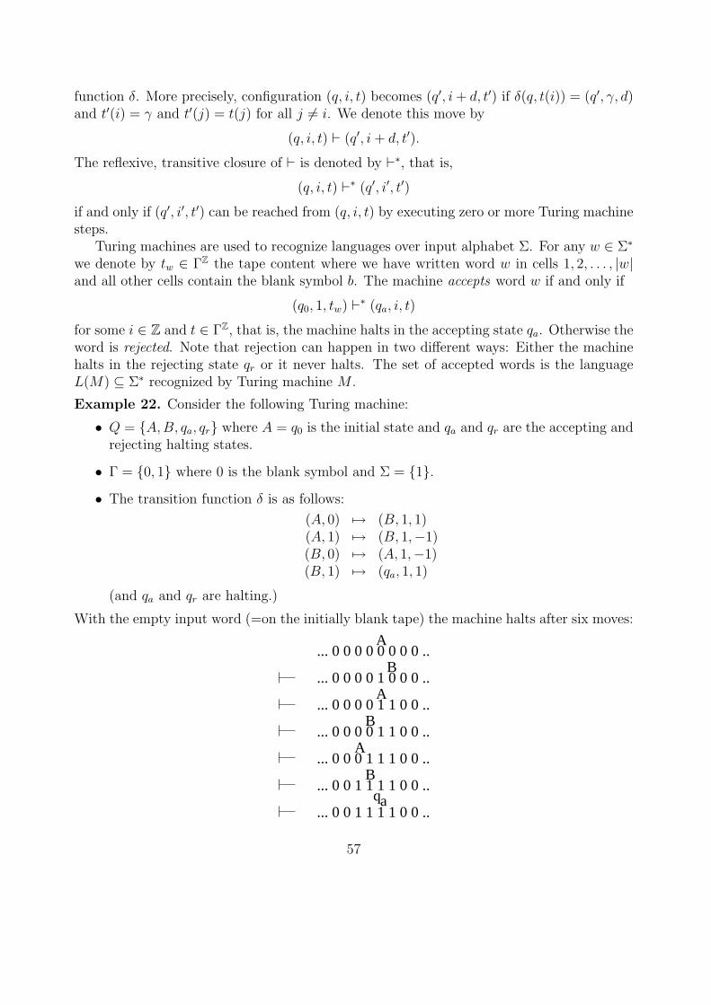
function δ. More precisely, configuration (q, i, t) becomes (q′, i + d, t′) if δ(q, t(i)) = (q′, γ, d)and t′(i) = γ and t′(j) = t(j) for all j 6= i. We denote this move by

(q, i, t) ` (q′, i + d, t′).

The reflexive, transitive closure of ` is denoted by `∗, that is,

(q, i, t) `∗ (q′, i′, t′)

if and only if (q′, i′, t′) can be reached from (q, i, t) by executing zero or more Turing machinesteps.

Turing machines are used to recognize languages over input alphabet Σ. For any w ∈ Σ∗

we denote by tw ∈ ΓZ the tape content where we have written word w in cells 1, 2, . . . , |w|and all other cells contain the blank symbol b. The machine accepts word w if and only if

(q0, 1, tw) `∗ (qa, i, t)

for some i ∈ Z and t ∈ ΓZ, that is, the machine halts in the accepting state qa. Otherwise theword is rejected. Note that rejection can happen in two different ways: Either the machinehalts in the rejecting state qr or it never halts. The set of accepted words is the languageL(M) ⊆ Σ∗ recognized by Turing machine M .

Example 22. Consider the following Turing machine:

• Q = A,B, qa, qr where A = q0 is the initial state and qa and qr are the accepting andrejecting halting states.

• Γ = 0, 1 where 0 is the blank symbol and Σ = 1.• The transition function δ is as follows:

(A, 0) 7→ (B, 1, 1)(A, 1) 7→ (B, 1,−1)(B, 0) 7→ (A, 1,−1)(B, 1) 7→ (qa, 1, 1)

(and qa and qr are halting.)

With the empty input word (=on the initially blank tape) the machine halts after six moves:

a

... 0 0 0 0 1 0 0 0 ...B

... 0 0 0 0 1 1 0 0 ...A

... 0 0 0 0 1 1 0 0 ...B

... 0 0 0 1 1 1 0 0 ...A

... 0 0 1 1 1 1 0 0 ...B

A... 0 0 0 0 0 0 0 0 ...

... 0 0 1 1 1 1 0 0 ...q

57

This example is a two-state busy beaver over the two letter alphabet: It runs on the initiallyblank tape for the longest possible time among all Turing machines that have two non-haltingstates and two tape letters, and that halt on the initially blank tape.

The numbers of moves by the three and four state busy beavers over the two letteralphabet are 21 and 107, respectively. The number of moves by five and six state busybeavers are not known but they are at least 47176870 and 102879, respectively. ¤

It is easy to see that the language recognized by a Turing machine is recursively enumer-able: For any Turing machine one can construct a semi-algorithm that simulates the Turingmachine step-by-step on any given input word until the word gets accepted. If the word isnot accepted then the semi-algorithm does not halt.

What is more complicated to see is that every recursively enumerable language is rec-ognized by a Turing machine. This is based on the fact that Turing machines — despitethe simplicity of their individual moves — can simulate the computation steps of arbitrary(semi-)algorithms. The proof of this fact is beyond the scope of the present notes:

Proposition 34 There is an algorithm that for any given (semi-)algorithm A whose inputis a word over alphabet Σ constructs a Turing machine M with the same input alphabet Σsuch that on every input w ∈ Σ∗

• if A returns ”yes” then M eventually enters its accepting state f ,

• if A returns ”no” then M eventually enters its rejecting state r, and

• if A does not halt then M does not halt either.

¤

From the proposition we directly get the following corollary:

Corollary 35 A language is recursively enumerable if and only if there is a Turing machinethat recognizes it. ¤

Consider then Turing machines that have the property that they halt on every input word.Such Turing machines only recognize recursive languages since an algorithm can simulatethem. Also the converse is true, as implied by Proposition 34:

Corollary 36 A language is recursive if and only if it is recognized by a Turing machinethat halts on every input word. ¤

Note: It is customary in the field of theoretical computer science to take Turing machines asthe formal definition of (semi)algorithms. In this case the above corollaries are definitions,and theorems can be stated to the effect that (semi)algorithms defined under other models(C-programs, for example) are equivalent to Turing machines. We did the process in reverse:

58

(semi)algorithms were defined in terms of C-programs, and the Corollaries above tie themto Turing machines.

Using Proposition 34 one can reduce decision problems concerning semi-algorithms intoanalogous questions concerning Turing machines. For example, undecidability of Semi-algorithm halting (Proposition 33) implies that it is undecidable if a given Turing machinehalts on a given input word. Undecidability of Sometimes halting (Example 21) implies that itis undecidable if a given Turing machine halts on some input. The most elementary problemconcerning Turing machines asks whether a given Turing machine halts when it is startedon the blank tape:

TM halting on blank tapeInstance: A Turing machine MProblem: Does M accept the empty input word ?

Proposition 37 The decision problem TM halting on blank tape is undecidable. More pre-cisely, it is semi-decidable while the complement problem is not semi-decidable.

Proof. The semi-decidability follows from an effective step-by-step simulation of the Turingmachine until (if ever) it halts. To prove undecidability we reduce Semi-algorithm halting.For any given semi-algorithm A and its input w we can effectively construct a semi-algorithmB that totally ignores its input u and simply calls A with input w. Clearly this B haltson all inputs (including the empty word) if A halts on input w and does not halt on anyinput (including the empty word) if A does not halt on input w. Using Proposition 34 weeffectively construct a Turing machine M that is equivalent to B. Machine M hence haltson the initially empty tape if and only if A halts on w. We have many-one reduced theundecidable problem Semi-algorithm halting into TM halting on blank tape. ¤

Example 23. Consider the following busy beaver function BB : N × N −→ N whereBB(n,m) is the largest number t such that there is a Turing machine with n non-haltingstates and m tape symbols that makes t moves on the blank tape and then halts. InExample 22 we discussed this function and mentioned that BB(2, 2) = 6, BB(3, 2) = 21,BB(4, 2) = 107, BB(5, 2) ≥ 47176870 and BB(6, 2) ≥ 102879. It follows from Proposition 37that BB grows faster than any function that can be computed. Namely, if there would be analgorithm A that outputs for any given n ∈ N and m ∈ N a value t such that BB(n,m) ≤ tthen this algorithm could be used to effectively solve TM halting on blank tape: For any givenTuring machine M we would namely obtain using algorithm A a number t such that if Mhalts on the blank tape, it does so within t steps. Then it is an easy matter to make thefirst t moves of M to see if it halts. It follows hence from Proposition 37 that algorithm Acannot exist.

Such functions that grow faster than any computable function are associated with allundecidable problems we encounter. ¤

59

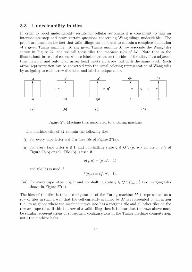
3.3 Undecidability in tiles

In order to proof undecidability results for cellular automata it is convenient to take anintermediate step and prove certain questions concerning Wang tilings undecidable. Theproofs are based on the fact that valid tilings can be forced to contain a complete simulationof a given Turing machine. To any given Turing machine M we associate the Wang tilesshown in Figure 27, and we call these tiles the machine tiles of M . Note that in theillustrations, instead of colors, we use labeled arrows on the sides of the tiles. Two adjacenttiles match if and only if an arrow head meets an arrow tail with the same label. Sucharrow representation can be converted into the usual coloring representation of Wang tilesby assigning to each arrow direction and label a unique color.

(d)

q

a

qaa

a qa qa

a’ a’

q’ q’ q

a

qa

(a) (b) (c)

Figure 27: Machine tiles associated to a Turing machine.

The machine tiles of M contain the following tiles:

(i) For every tape letter a ∈ Γ a tape tile of Figure 27(a),

(ii) For every tape letter a ∈ Γ and non-halting state q ∈ Q \ qa, qr an action tile ofFigure 27(b) or (c). Tile (b) is used if

δ(q, a) = (q′, a′,−1)

and tile (c) is used ifδ(q, a) = (q′, a′, +1).

(iii) For every tape letter a ∈ Γ and non-halting state q ∈ Q \ qa, qr two merging tilesshown in Figure 27(d).

The idea of the tiles is that a configuration of the Turing machine M is represented as arow of tiles in such a way that the cell currently scanned by M is represented by an actiontile, its neighbor where the machine moves into has a merging tile and all other tiles on therow are tape tiles. If this is a row of a valid tiling then it is clear that the rows above mustbe similar representations of subsequent configurations in the Turing machine computation,until the machine halts.

60

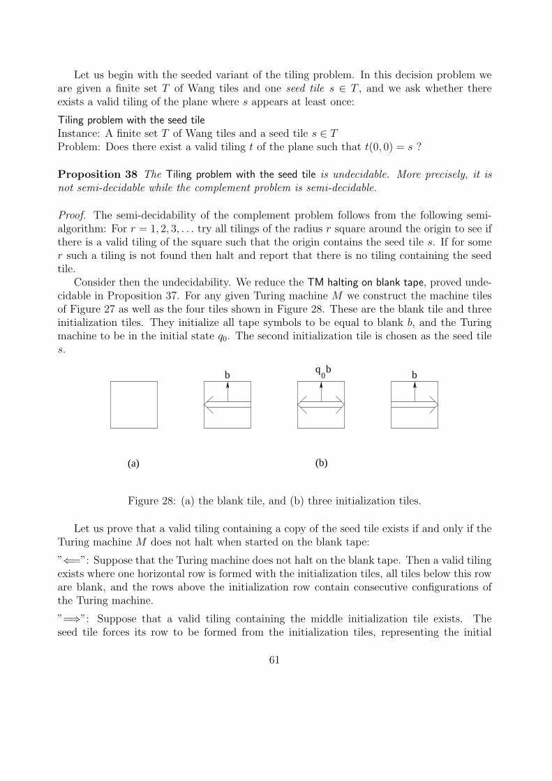
Let us begin with the seeded variant of the tiling problem. In this decision problem weare given a finite set T of Wang tiles and one seed tile s ∈ T , and we ask whether thereexists a valid tiling of the plane where s appears at least once:

Tiling problem with the seed tileInstance: A finite set T of Wang tiles and a seed tile s ∈ TProblem: Does there exist a valid tiling t of the plane such that t(0, 0) = s ?

Proposition 38 The Tiling problem with the seed tile is undecidable. More precisely, it isnot semi-decidable while the complement problem is semi-decidable.

Proof. The semi-decidability of the complement problem follows from the following semi-algorithm: For r = 1, 2, 3, . . . try all tilings of the radius r square around the origin to see ifthere is a valid tiling of the square such that the origin contains the seed tile s. If for somer such a tiling is not found then halt and report that there is no tiling containing the seedtile.

Consider then the undecidability. We reduce the TM halting on blank tape, proved unde-cidable in Proposition 37. For any given Turing machine M we construct the machine tilesof Figure 27 as well as the four tiles shown in Figure 28. These are the blank tile and threeinitialization tiles. They initialize all tape symbols to be equal to blank b, and the Turingmachine to be in the initial state q0. The second initialization tile is chosen as the seed tiles.

0

(a) (b)

q bb b

Figure 28: (a) the blank tile, and (b) three initialization tiles.

Let us prove that a valid tiling containing a copy of the seed tile exists if and only if theTuring machine M does not halt when started on the blank tape:

”⇐=”: Suppose that the Turing machine does not halt on the blank tape. Then a valid tilingexists where one horizontal row is formed with the initialization tiles, all tiles below this roware blank, and the rows above the initialization row contain consecutive configurations ofthe Turing machine.

”=⇒”: Suppose that a valid tiling containing the middle initialization tile exists. Theseed tile forces its row to be formed from the initialization tiles, representing the initial

61

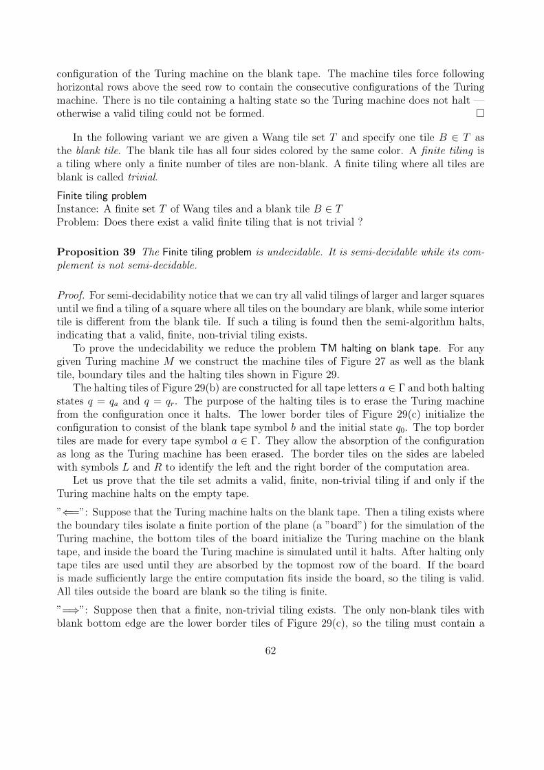
configuration of the Turing machine on the blank tape. The machine tiles force followinghorizontal rows above the seed row to contain the consecutive configurations of the Turingmachine. There is no tile containing a halting state so the Turing machine does not halt —otherwise a valid tiling could not be formed. ¤

In the following variant we are given a Wang tile set T and specify one tile B ∈ T asthe blank tile. The blank tile has all four sides colored by the same color. A finite tiling isa tiling where only a finite number of tiles are non-blank. A finite tiling where all tiles areblank is called trivial.

Finite tiling problemInstance: A finite set T of Wang tiles and a blank tile B ∈ TProblem: Does there exist a valid finite tiling that is not trivial ?

Proposition 39 The Finite tiling problem is undecidable. It is semi-decidable while its com-plement is not semi-decidable.

Proof. For semi-decidability notice that we can try all valid tilings of larger and larger squaresuntil we find a tiling of a square where all tiles on the boundary are blank, while some interiortile is different from the blank tile. If such a tiling is found then the semi-algorithm halts,indicating that a valid, finite, non-trivial tiling exists.

To prove the undecidability we reduce the problem TM halting on blank tape. For anygiven Turing machine M we construct the machine tiles of Figure 27 as well as the blanktile, boundary tiles and the halting tiles shown in Figure 29.

The halting tiles of Figure 29(b) are constructed for all tape letters a ∈ Γ and both haltingstates q = qa and q = qr. The purpose of the halting tiles is to erase the Turing machinefrom the configuration once it halts. The lower border tiles of Figure 29(c) initialize theconfiguration to consist of the blank tape symbol b and the initial state q0. The top bordertiles are made for every tape symbol a ∈ Γ. They allow the absorption of the configurationas long as the Turing machine has been erased. The border tiles on the sides are labeledwith symbols L and R to identify the left and the right border of the computation area.

Let us prove that the tile set admits a valid, finite, non-trivial tiling if and only if theTuring machine halts on the empty tape.

”⇐=”: Suppose that the Turing machine halts on the blank tape. Then a tiling exists wherethe boundary tiles isolate a finite portion of the plane (a ”board”) for the simulation of theTuring machine, the bottom tiles of the board initialize the Turing machine on the blanktape, and inside the board the Turing machine is simulated until it halts. After halting onlytape tiles are used until they are absorbed by the topmost row of the board. If the boardis made sufficiently large the entire computation fits inside the board, so the tiling is valid.All tiles outside the board are blank so the tiling is finite.

”=⇒”: Suppose then that a finite, non-trivial tiling exists. The only non-blank tiles withblank bottom edge are the lower border tiles of Figure 29(c), so the tiling must contain a

62

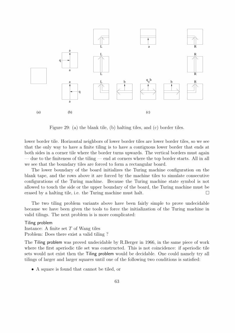
q

q b0 b

L

L

L

(b)(a)

bL R

R

R

Ra

(c)

a

q

a

a

a

Figure 29: (a) the blank tile, (b) halting tiles, and (c) border tiles.

lower border tile. Horizontal neighbors of lower border tiles are lower border tiles, so we seethat the only way to have a finite tiling is to have a contiguous lower border that ends atboth sides in a corner tile where the border turns upwards. The vertical borders must again— due to the finiteness of the tiling — end at corners where the top border starts. All in allwe see that the boundary tiles are forced to form a rectangular board.

The lower boundary of the board initializes the Turing machine configuration on theblank tape, and the rows above it are forced by the machine tiles to simulate consecutiveconfigurations of the Turing machine. Because the Turing machine state symbol is notallowed to touch the side or the upper boundary of the board, the Turing machine must beerased by a halting tile, i.e. the Turing machine must halt. ¤

The two tiling problem variants above have been fairly simple to prove undecidablebecause we have been given the tools to force the initialization of the Turing machine invalid tilings. The next problem is is more complicated:

Tiling problemInstance: A finite set T of Wang tilesProblem: Does there exist a valid tiling ?

The Tiling problem was proved undecidable by R.Berger in 1966, in the same piece of workwhere the first aperiodic tile set was constructed. This is not coincidence: if aperiodic tilesets would not exist then the Tiling problem would be decidable. One could namely try alltilings of larger and larger squares until one of the following two conditions is satisfied:

• A square is found that cannot be tiled, or

63

• A tiling of a square is found where the top and the bottom colors match and left andthe right sides match.

The first condition happens if and only if no valid tiling of the plane exists, and the secondcondition is satisfied if and only if a periodic tiling exists. If aperiodic tile sets did notexist then one of the two conditions would always be satisfied, and this would provide thenan algorithm for the Tiling problem. But aperiodic tile sets fail to satisfy either of the twoconditions.

We state Berger’s result without a proof (it has been proven in the Tilings and Patternsclass). In fact, an even stronger variant will be used in the next section:

NW-deterministic tiling problemInstance: A NW-deterministic set T of Wang tilesProblem: Does there exist a valid tiling ?

Proposition 40 The NW-deterministic tiling problem is undecidable. More precisely, theproblem is not semi-decidable but its complement is semi-decidable. ¤Finally, as the last variant of the tiling problem we state without a proof the undecidabilityof the problem that asks whether a given tile set admits a periodic tiling:

Periodic tiling problemInstance: A finite set T of Wang tilesProblem: Does there exist a valid periodic tiling ?

Proposition 41 The Periodic tiling problem is undecidable. More precisely, the problem issemi-decidable while its complement is not. ¤

3.4 Undecidable questions concerning cellular automata

Next we turn to our main topic and prove several questions concerning cellular automataundecidable. The input instance to these decision problems include a cellular automaton.The problems typically concern properties of its global function G. We usually state thatthe instance of a problem is a CA function G, but one should keep in mind that, in fact, theinput instance is given in terms of the local rule that specifies G.

We start with a problem of deciding if a given CA function has trivial behavior. A CAfunction G is called nilpotent if all configurations eventually lead to the quiescent configura-tion. In fact, then there is a constant n ∈ Z+ such that Gn(c) is the quiescent configurationfor all c ∈ SZ

d. To see this, consider a transitive configuration t ∈ SZ

dthat contains a

copy of every finite pattern as a subpattern, and choose n such that Gn(t) is the quiescentconfiguration. It is easy to see that with this choice of n configuration Gn(c) is quiescent forall c ∈ SZ

d.

2D nilpotencyInstance: A two-dimensional cellular automaton GProblem: Is G nilpotent ?

64

Proposition 42 Decision problem 2D nilpotency is undecidable. It is semi-decidable whilethe complement is not semi-decidable.

Proof. For semi-decidability notice that, for n = 1, 2, 3 . . ., we can effectively construct acellular automaton whose global function is Gn and check whether the local rule of the CAmaps everything into the quiescent state. If that happens for some n then we halt and reportthat the CA is nilpotent.

To prove undecidability we reduce the Tiling problem. For any given Wang tile set T weconstruct a cellular automaton whose state set is S = T ∪ q and the local rule turns a cellinto state q except if the cell and its four neighbors are tiles that match in color, in whichcase the state is not changed. (This same construction was already used in Example 17).Let us prove that the CA is not nilpotent if and only if T admits a valid tiling.

”⇐=”: Suppose a valid tiling exists. This tiling, as a configuration of the CA, is a fixedpoint so it never becomes quiescent. The CA is not nilpotent.

”=⇒”: Suppose no valid tiling exists. Then there is number n such that no valid tiling ofan n× n square exists. This means that after the first application of the CA, regardless ofthe initial configuration, state q appears in every n × n square. Since state q spreads it isclear that the configuration becomes eventually quiescent. Hence the CA is nilpotent. ¤

In fact, using the undecidability of the NW-deterministic tiling problem, we can prove thatthe nilpotency problem is undecidable even for one-dimensional CA:

1D nilpotencyInstance: A one-dimensional cellular automaton GProblem: Is G nilpotent ?

Proposition 43 Decision problem 1D nilpotency is undecidable. It is semi-decidable whilethe complement is not semi-decidable.

Proof. Semi-decidability follows in the same way as in the two-dimensional case. Toprove undecidability we reduce the NW-deterministic tiling problem. Let T be a given NW-deterministic tile set. We construct a one-dimensional CA whose state set is S = T ∪q andthe local rule turns a cell into state q except in the case that the cell and its right neighborare in states x, y ∈ T , respectively, and tile z ∈ T exists so that tiles x, y, z match as inFigure 24(a). In this case z is the new state of the cell. This same construction was alreadyused in Example 18.

Let us prove that the CA is not nilpotent if and only if T admits a valid tiling.

”⇐=”: Suppose a valid tiling exists. If c ∈ T Z is a diagonal of this tiling then the configura-tions Gn(c) in its orbit are subsequent diagonals of the same tiling, for all n = 1, 2, . . .. Thismeans that c never becomes quiescent, and the CA is not nilpotent.

65

”=⇒”: Suppose no valid tiling exists. Then there is number n such that no valid tiling of ann×n square exists. This means that for every initial configuration c ∈ SZ the configurationG2n(c) is quiescent: If it is not quiescent then a valid tiling of an n× n square can be readfrom the space time diagram of configurations c,G(c), . . . , G2n(c). We conclude that the CAis nilpotent. ¤

Consider then the problem of determining if a given two-dimensional CA is surjective. Toprove that this question is undecidable we reduce the Finite tiling problem. In the reductionwe need a particular set D of 23 Wang tiles shown in Figure 30. The topmost tile is calledblank. All other tiles have a unique incoming and outgoing arrow. In valid tilings arrowsand labels must match. The non-blank tiles are considered directed: the follower of a tileis the neighbor directed to by the outgoing arrow on the tile. Since each non-blank tile hasexactly one incoming arrow, it is clear that if the tiling is valid at a tile then the tile is thefollower of exactly one of its four neighbors.

The tile at the center in Figure 30 where the dark and light thick horizontal lines meet iscalled the cross. It has a special role in the forthcoming proof. A rectangular loop is a validtiling of a rectangle using tiles in D where the follower path forms a loop that visits everytile of the rectangle, and the outside border of the rectangle is colored blank. See Figure 31for an example of a rectangular loop through a rectangle of size 12× 7. (The edge labels arenot shown for the sake of clarity of the figure.) It is easy to see that a rectangular loop ofsize 2n×m exist for all n ≥ 2 and m ≥ 3. Any tile in an even column in the interior of therectangle can be made to contain the unique cross of the rectangular loop.

The tile set D has a property that resembles the plane-filling property:

Lemma 44 Let t ∈ DZ2be a tiling, and ~p1, ~p2, ~p3, . . . a path in t such that the tiling t is

valid at ~pi for all i = 1, 2, 3, . . .. If the path covers only a finite number of different cells thenthe cells on the path form a rectangular loop.

Proof. Because the path only covers a finite number of different cells, the path must form acycle. A cycle must contain arrows in all four directions. In particular, an arrow to the leftmust appear. Only the tiles at the bottom row of Figure 30 involve left arrows, so the pathmust contain a horizontal segment of left arrows that ends in a lower left corner tile wherethe path turns upwards and has label SW. From there on the label SW forces the path tocontinue upwards (forming the left border of the rectangle) until it turns to the right, withlabel A. In this vertical segment the label of the arrow must change from SW to NW, soa unique horizontal dark thick line gets initiated. Label A forces the path to immediatelyturn down. The path can only continue downwards until it eventually turns when the tilebelow has label C. The only tile with label C on the top edge contains a left arrow, so thetile must be next to the lower left corner tile.

Next the path has no other choice but to turn up and to continue upwards until it reachesthe top of the rectangle where label B on its left side forces it to turn right. Continuationof the same reasoning shows that the path must continue up and down filling the rectangleuntil at some point the downward path has labels NE. This label must be changed to SE at

66

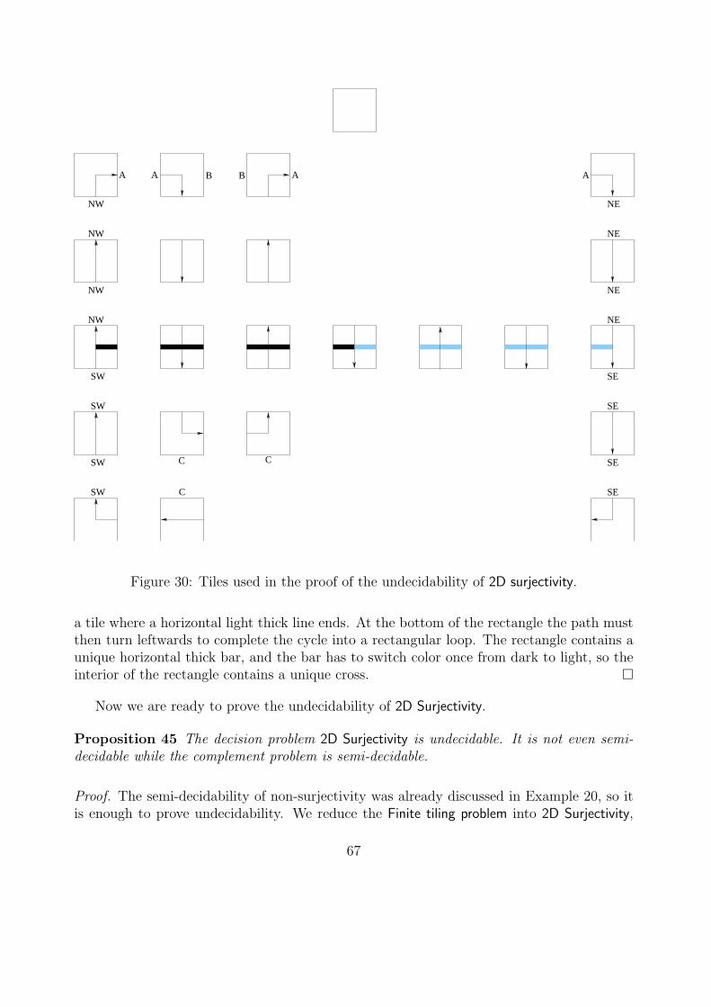
A

SW

NW

NW

NW

NW

SW

SW

SW

NE

NE

SE

NE

NE

SE

SE

SE

A A B B A

C

C

C

Figure 30: Tiles used in the proof of the undecidability of 2D surjectivity.

a tile where a horizontal light thick line ends. At the bottom of the rectangle the path mustthen turn leftwards to complete the cycle into a rectangular loop. The rectangle contains aunique horizontal thick bar, and the bar has to switch color once from dark to light, so theinterior of the rectangle contains a unique cross. ¤

Now we are ready to prove the undecidability of 2D Surjectivity.

Proposition 45 The decision problem 2D Surjectivity is undecidable. It is not even semi-decidable while the complement problem is semi-decidable.

Proof. The semi-decidability of non-surjectivity was already discussed in Example 20, so itis enough to prove undecidability. We reduce the Finite tiling problem into 2D Surjectivity,

67

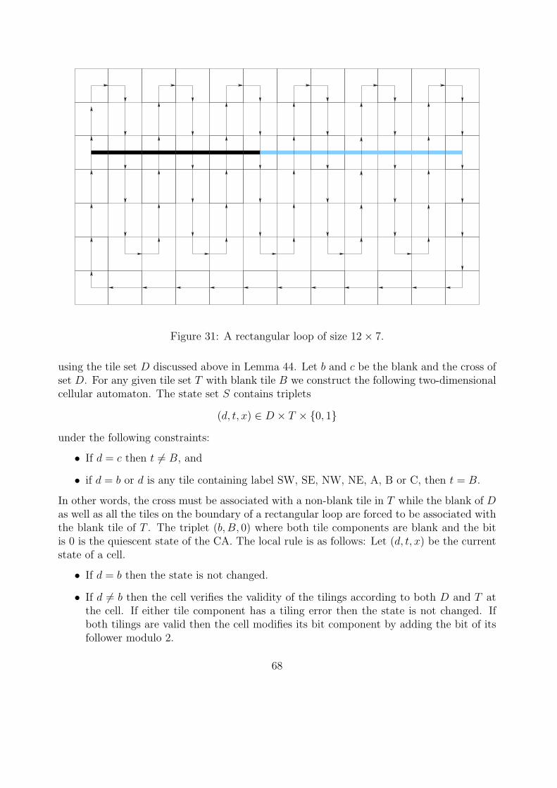
Figure 31: A rectangular loop of size 12× 7.

using the tile set D discussed above in Lemma 44. Let b and c be the blank and the cross ofset D. For any given tile set T with blank tile B we construct the following two-dimensionalcellular automaton. The state set S contains triplets

(d, t, x) ∈ D × T × 0, 1under the following constraints:

• If d = c then t 6= B, and

• if d = b or d is any tile containing label SW, SE, NW, NE, A, B or C, then t = B.

In other words, the cross must be associated with a non-blank tile in T while the blank of Das well as all the tiles on the boundary of a rectangular loop are forced to be associated withthe blank tile of T . The triplet (b, B, 0) where both tile components are blank and the bitis 0 is the quiescent state of the CA. The local rule is as follows: Let (d, t, x) be the currentstate of a cell.

• If d = b then the state is not changed.

• If d 6= b then the cell verifies the validity of the tilings according to both D and T atthe cell. If either tile component has a tiling error then the state is not changed. Ifboth tilings are valid then the cell modifies its bit component by adding the bit of itsfollower modulo 2.

68

Let us prove that this CA is not surjective if and only if T admits a valid, finite, non-trivialtiling.

”⇐=”: Suppose a valid, finite, non-trivial tiling t ∈ T Z2

exists. Consider a configuration ofthe CA whose T -components form the valid tiling t and the D-components form a rectangularloop whose interior covers all non-blank elements of t. Tiles outside the rectangle are allblank and have bit 0. The cross can be positioned so that it is in the same cell as somenon-blank tile in t. In such a configuration both T and D tilings are everywhere valid. TheCA updates the bits of all tiles in the rectangular loop by performing modulo 2 addi tionwith their followers, while the bits outside the rectangle remain 0. We get two differentconfigurations that have the same image: In c0 all bits in the rectangle are equal to 0 whilein c1 they are all equal to 1. The local rule updates the bits so that G(c0) = G(c1) = c0.Configurations c0 and c1 only differ in a finite number of cells, so it follows from the Garden-of-Eden theorem (Proposition 18) that G is not surjective.

”=⇒”: Suppose then that the CA is not surjective. According to the Garden-of-Edentheorem (Proposition 16) there are two different finite configurations c0 and c1 such thatG(c0) = G(c1). Since only bit components of states are changed, the tilings in c0 andc1 according to D- and T -components of the states are identical. There is a cell ~p1 suchthat c0 and c1 have different bits at cell ~p1. Since these bits become identical in the nextconfiguration, the D-tiling must be correct at ~p1 and c0 and c1 must have different bits in thefollower position ~p2. We repeat the reasoning and obtain an infinite sequence of positions~p1, ~p2, ~p3, . . . such that each ~pi+1 is the follower of ~pi, and the D tiling is correct at each ~pi.Moreover, c0 and c1 have different bits in each position ~pi. Because configurations c0 and c1

are finite we see that the path can only contain a finite number of distinct cells. It followsthen from Lemma 44 that the path must form a valid rectangular loop.

Also the tiling according to the T -components must be valid at each cell of the path.Because of the constraints on the allowed triplets, the T -components on the boundary of therectangle are the blank B, while the cross in the interior contains a non-blank element of T .Hence there is a valid tiling of a rectangle according to T that contains a non-blank tile andhas a blank boundary. This means that a finite, valid and non-trivial tiling is possible.

¤

Finally, consider the problem of determining if a given two-dimensional CA is reversible.The proof of its undecidability is similar to the previous proof. Only, instead of the Finitetiling problem we use the Tiling problem, and the special set D if directed tiles is replaced bya tile set with the plane filling property.

Proposition 46 Decision problem 2D Reversibility is undecidable. It is semi-decidable whilethe complement problem is not.

Proof. The semi-decidability was already shown in Example 20. Let us prove 2D Reversibilityundecidable by reducing the Tiling problem into it. In the reduction we use a set D of directed

69

tiles that has the plane filling property. The existence of such D was stated (without proof)in Proposition 32.

Let T be a given set of Wang tiles that is an instance of the Tiling problem. One caneffectively construct a two-dimensional CA whose state set is

S = T ×D × 0, 1

and the local rule updates the bit component of a cell as follows:

• If either the T - or the D-components contain a tiling error at the cell then the stateof the cell is not changed, but

• if the tilings according to both T - and D-components are valid at the cell then the bitof the follower cell (according to the direction in the D-component) is added to thepresent bit value modulo 2.

The tile components are not changed. Let us prove that this CA is not injective (and hencenot reversible) if and only if T admits a valid tiling.

”⇐=”: Suppose a valid tiling exists. Construct two configurations c0 and c1 where the T -and D-components form the same valid tilings t ∈ T Z

2and d ∈ DZ2

, respectively. In c0

all bits are 0 while in c1 they are all 1. Since the tilings are everywhere valid, every cellperforms modulo 2 addition of two bits, which means that every bit becomes 0. HenceG(c0) = G(c1) = c0, and G is not injective.

”=⇒”: Suppose then that the CA is not injective. There are two different configurations c0

and c1 such that G(c0) = G(c1). Tile components are not modified by the CA so they areidentical in c0 and c1. There is a cell ~p1 such that c0 and c1 have different bits at cell ~p1.Since these bits become identical in the next configuration, the D-tiling must be correct at~p1 and c0 and c1 must have different bits in the follower position ~p2. We repeat the reasoningand obtain an infinite sequence of positions ~p1, ~p2, ~p3, . . . such that each ~pi+1 is the followerof ~pi, and the D tiling is correct at each ~pi. It follows from the plane filling property ofD that path ~p1, ~p2, ~p3, . . . covers arbitrarily large squares. Also the tiling according to theT -components must be valid at each cell of the path. Hence tile set T admits valid tilingsof arbitrarily large squares, and therefore it admits a valid tiling of the entire plane.

¤

Note: The two-dimensional cellular automata that we constructed in the proofs of Propo-sitions 42, 45 and 46 use the von Neumann neighborhood. So the decision problems 2DNilpotency, 2D Surjectivity and 2D Reversibility are undecidable even when the input instanceis restricted to CA with the von Neumann neighborhood.

The one-dimensional CA constructed in the proof of Proposition 43 has radius-12

neigh-borhood. Also, the quiescent state q is spreading: Any cell whose neighborhood containsstate q turns to state q. So the decision problem 1D Nilpotency is undecidable among radius-1

2

CA that have a spreading state.

70

Another fact to observe is that all undecidability results of this section apply to d-dimensional CA for any d ≥ 2, even though we only proved them in the case d = 2. Namely,for any d > 2 a given two-dimensional CA A can be converted into a d-dimensional CAconsisting of a (d−2)-dimensional grid of independent two-dimensional layers, each of whichoperates as A. This d-dimensional CA is nilpotent, surjective or reversible if and only if Ais nilpotent, surjective or reversible, respectively.

We finish this section by defining busy beaver -like, very rapidly growing functions asso-ciated with the undecidable decision problems above.

Example 24. Let us define following functions n, s, r : Z+ −→ Z+: For every k ∈ Z+

• n(k) is the largest t such that there is a nilpotent, one-dimensional, radius-12

cellularautomaton G with k states, and a configuration c such that Gt(c) is not the quiescentconfiguration.

• s(k) is largest t such that there is a non-surjective, two-dimensional CA that uses thevon Neumann neighborhood and has k states, such that there is no orphan pattern ofsize t× t.

• r(k) is the largest t such that there is a reversible, two-dimensional CA G with k statesand the von Neumann neighborhood such that the inverse of G is not obtained usingthe radius-t neighborhood.

Each of the functions is well defined since its value for any k is the maximum among a finitenumber of positive integers. Yet no algorithm can compute an upper bound for any of thefunctions. If some algorithm could produce for every given k a number t such that n(k) ≤ t,s(k) ≤ t or r(k) ≤ t then this algorithm could be used to solve the decision problem 1DNilpotency, 2D Surjectivity or 2D Reversibility, respectively. In each case such value t wouldnamely provide a bound on the size of instances that the corresponding semi-algorithm needsto check.

We conclude that there are nilpotent CA that have configurations that survive very longtime before becoming quiescent, there are non-surjective CA whose smallest orphan is verylarge, and there are reversible CA whose inverse CA have very large neighborhoods. ¤

3.5 Computational universality

General purpose computers are computationally universal: they can simulate any semi-algorithm if the semi-algorithm is encoded properly and is included as part of the input.Note how important it is for us that computational universality is at all possible – otherwisewe would have to build a new computer for each computational task!

A recursively enumerable language L ⊆ Σ∗ is r.e.-complete if every recursively enumerablelanguage is many-one reducible to L. In other words, for every r.e. language K ⊆ ∆∗ thereexists an algorithm that takes as input an arbitrary word u ∈ ∆∗ and outputs a word v ∈ Σ∗

with the property that u ∈ K if and only if v ∈ L. In terms of decision problems, we call a

71

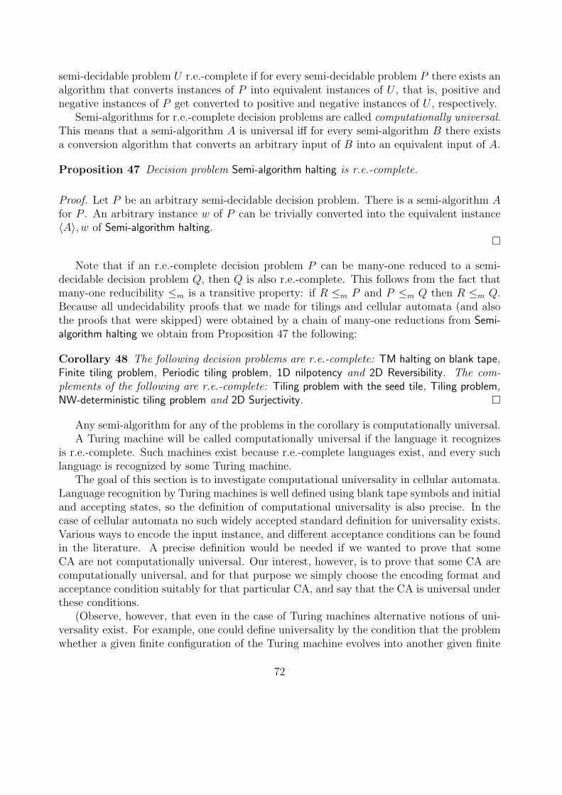
semi-decidable problem U r.e.-complete if for every semi-decidable problem P there exists analgorithm that converts instances of P into equivalent instances of U , that is, positive andnegative instances of P get converted to positive and negative instances of U , respectively.

Semi-algorithms for r.e.-complete decision problems are called computationally universal.This means that a semi-algorithm A is universal iff for every semi-algorithm B there existsa conversion algorithm that converts an arbitrary input of B into an equivalent input of A.

Proposition 47 Decision problem Semi-algorithm halting is r.e.-complete.

Proof. Let P be an arbitrary semi-decidable decision problem. There is a semi-algorithm Afor P . An arbitrary instance w of P can be trivially converted into the equivalent instance〈A〉, w of Semi-algorithm halting.

¤

Note that if an r.e.-complete decision problem P can be many-one reduced to a semi-decidable decision problem Q, then Q is also r.e.-complete. This follows from the fact thatmany-one reducibility ≤m is a transitive property: if R ≤m P and P ≤m Q then R ≤m Q.Because all undecidability proofs that we made for tilings and cellular automata (and alsothe proofs that were skipped) were obtained by a chain of many-one reductions from Semi-algorithm halting we obtain from Proposition 47 the following:

Corollary 48 The following decision problems are r.e.-complete: TM halting on blank tape,Finite tiling problem, Periodic tiling problem, 1D nilpotency and 2D Reversibility. The com-plements of the following are r.e.-complete: Tiling problem with the seed tile, Tiling problem,NW-deterministic tiling problem and 2D Surjectivity. ¤

Any semi-algorithm for any of the problems in the corollary is computationally universal.A Turing machine will be called computationally universal if the language it recognizes

is r.e.-complete. Such machines exist because r.e.-complete languages exist, and every suchlanguage is recognized by some Turing machine.

The goal of this section is to investigate computational universality in cellular automata.Language recognition by Turing machines is well defined using blank tape symbols and initialand accepting states, so the definition of computational universality is also precise. In thecase of cellular automata no such widely accepted standard definition for universality exists.Various ways to encode the input instance, and different acceptance conditions can be foundin the literature. A precise definition would be needed if we wanted to prove that someCA are not computationally universal. Our interest, however, is to prove that some CA arecomputationally universal, and for that purpose we simply choose the encoding format andacceptance condition suitably for that particular CA, and say that the CA is universal underthese conditions.

(Observe, however, that even in the case of Turing machines alternative notions of uni-versality exist. For example, one could define universality by the condition that the problemwhether a given finite configuration of the Turing machine evolves into another given finite

72

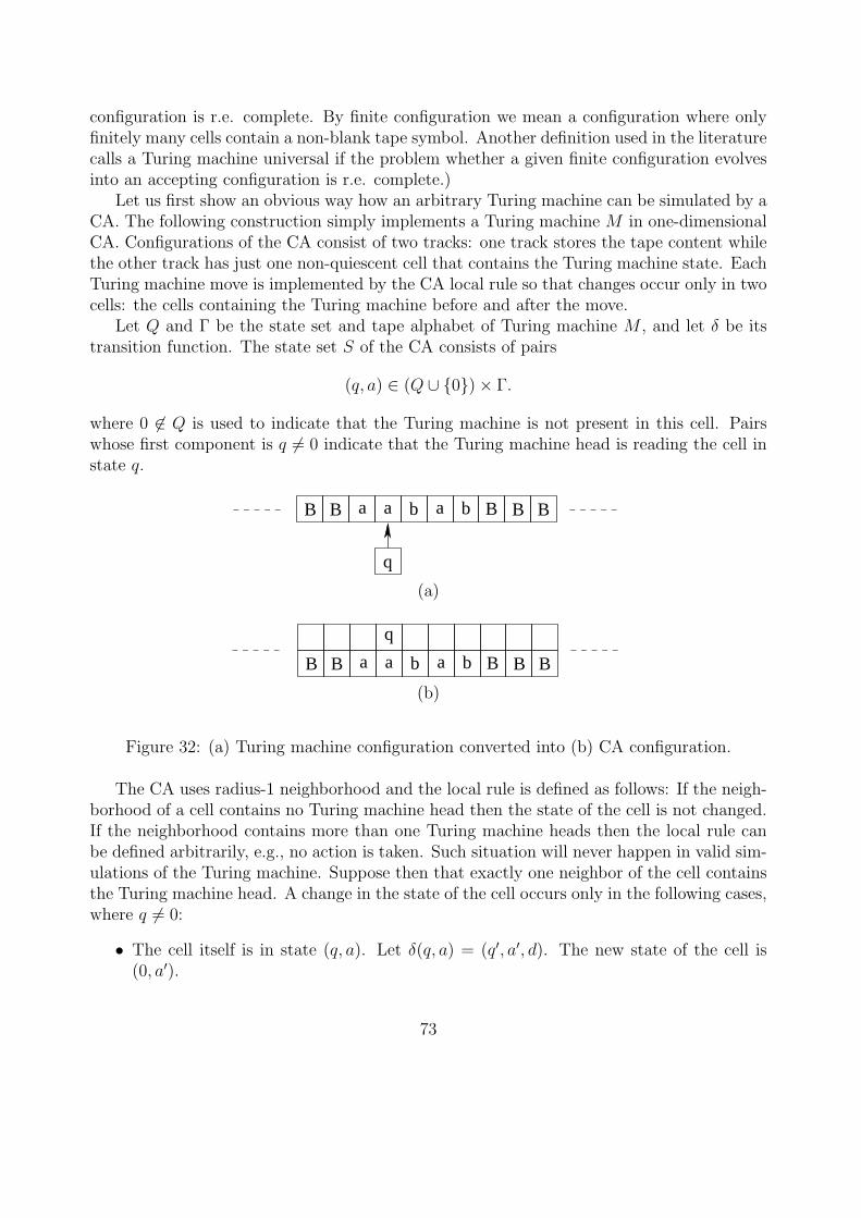
configuration is r.e. complete. By finite configuration we mean a configuration where onlyfinitely many cells contain a non-blank tape symbol. Another definition used in the literaturecalls a Turing machine universal if the problem whether a given finite configuration evolvesinto an accepting configuration is r.e. complete.)

Let us first show an obvious way how an arbitrary Turing machine can be simulated by aCA. The following construction simply implements a Turing machine M in one-dimensionalCA. Configurations of the CA consist of two tracks: one track stores the tape content whilethe other track has just one non-quiescent cell that contains the Turing machine state. EachTuring machine move is implemented by the CA local rule so that changes occur only in twocells: the cells containing the Turing machine before and after the move.

Let Q and Γ be the state set and tape alphabet of Turing machine M , and let δ be itstransition function. The state set S of the CA consists of pairs

(q, a) ∈ (Q ∪ 0)× Γ.

where 0 6∈ Q is used to indicate that the Turing machine is not present in this cell. Pairswhose first component is q 6= 0 indicate that the Turing machine head is reading the cell instate q.

q

a a b a bB B B B B

(a)

B

q

a a b a bB B B B

(b)

Figure 32: (a) Turing machine configuration converted into (b) CA configuration.

The CA uses radius-1 neighborhood and the local rule is defined as follows: If the neigh-borhood of a cell contains no Turing machine head then the state of the cell is not changed.If the neighborhood contains more than one Turing machine heads then the local rule canbe defined arbitrarily, e.g., no action is taken. Such situation will never happen in valid sim-ulations of the Turing machine. Suppose then that exactly one neighbor of the cell containsthe Turing machine head. A change in the state of the cell occurs only in the following cases,where q 6= 0:

• The cell itself is in state (q, a). Let δ(q, a) = (q′, a′, d). The new state of the cell is(0, a′).

73

• The right neighbor is in state (q, a) and δ(q, a) = (q′, a′,−1). Then the new state ofthe cell will be (q′, x) where (0, x) is its old state.

• The left neighbor is in state (q, a) and δ(q, a) = (q′, a′, +1). Then the new state of thecell will be (q′, x) where (0, x) is its old state.

The quiescent state of the CA is the pair (0, B) where B is the blank tape symbol of theTuring machine.

Let us encode Turing machine configurations as CA configurations as follows: For allq ∈ Q, i ∈ Z and t ∈ ΓZ the Turing machine configuration (q, i, t) is encoded as the CAconfiguration c ∈ SZ where for every j ∈ Z

c(j) =

(q, t(j)) if j = i,(0, t(j)) if j 6= i.

Let us denote thenc = E(q, i, t)

and callE : Q× Z× ΓZ −→ SZ

the encoding function. See Figure 32 for an illustration for the encoding of a configuration.It is clear from the definition of the CA that the diagram

Q× Z× ΓZ` - Q× Z× ΓZ

SZ

E

? G - SZ

E

?

commutes. In other words, if the Turing machine changes (q, i, t) into (q′, i′, t′) in k stepsthen the CA changes configuration E(q, i, t) into E(q′, i′, t′) in k steps. This means that theCA simulates the Turing machine moves. If the Turing machine M that the constructionwas performed on is computationally universal then the resulting CA can be called com-putationally universal as well. In this form of universality the input word is encoded as afinite initial configuration, and the word is accepted if a configuration with some cell in state(qa, x) for some x ∈ Γ is eventually reached, where qa is the accepting state of the Turingmachine.

Proposition 49 There is a one-dimensional CA and a subset F ⊆ S of states such that thefollowing decision problem is r.e. complete: ”Does a given finite configuration c evolve intoa configuration where some cell is in state belonging to F ?”

74

Proof. Clearly the given decision problem is semi-decidable for any CA. The completenessis proved by performing the construction above for a Turing machine M that recognizes anr.e. complete language L ⊆ Σ∗ and by choosing

F = (qa, x) | x ∈ Γ.Then for any w ∈ Σ∗ we have w ∈ L if and only if the finite configuration c = E(q0, 1, tw) isa positive instance of the given decision problem, where q0 is the initial state of the Turingmachine, and tw ∈ ΓZ has word w written in positions 1, 2, . . . , |w| and blank B in all othercells. ¤

It is an easy matter to modify the CA for alternative forms of universality. The followingproposition lists a few possibilities:

Proposition 50 For each of the following decision problems there is a one-dimensional CAsuch that the given decision problem is r.e. complete:

(a) Does a given finite configuration c evolve into the quiescent configuration ?

(b) For a fixed spreading state s, does a given finite configuration c evolve into a configu-ration e in which state s appears ?

(c) Does a given finite configuration c evolve into a fixed point ?

(d) Given two finite configurations c and e, does c evolve into e, that is, does there existn ≥ 0 such that Gn(c) = e ?

Proof. First note that all questions (a)–(d) are semi-decidable, so it is enough to showcompleteness.

Consider a universal Turing machine that has the property that it never writes the blanksymbol B. Such Turing machine is easily obtained from any universal machine by introducinga new symbol B′ that behaves exactly as B, and the Turing machine always writes B′ onthe tape instead of B. This modification is done so that we can easily recognize the activepart of the tape.

Let us modify the previous construction of the CA A that simulates a universal Turingmachine:

For (a) we modify A it so that if an accepting state in F appears, it immediately sends twosignals, one to the left and another one to the right, that change all states into the quiescentstate. When the signal reaches the quiescent state (indicating that the active part of thetape ends) the signal disappears.

For (b) we modify A so that we introduce new spreading state s, and modify the local ruleso that states in F become s, regardless of their neighbors.

For (c) we introduce a new inactive state s. Cell in state s remains s and also all itsneighbors do not change their states. States in F become this s in one step. Then accepting

75

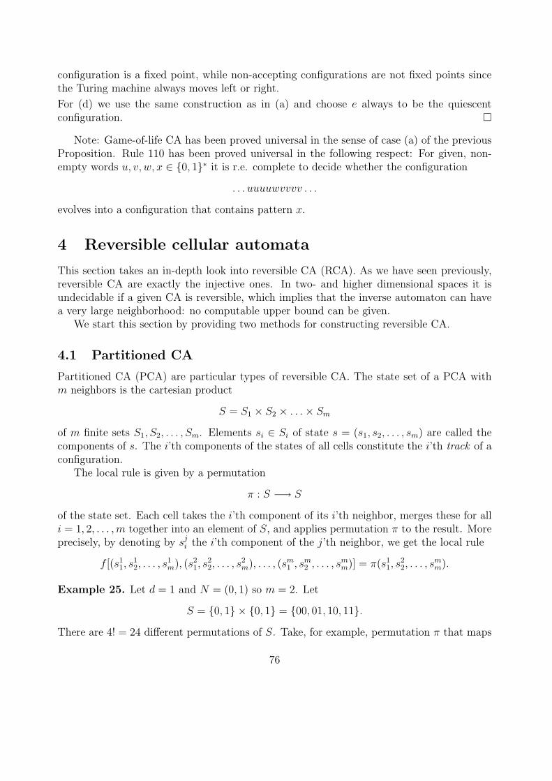
configuration is a fixed point, while non-accepting configurations are not fixed points sincethe Turing machine always moves left or right.

For (d) we use the same construction as in (a) and choose e always to be the quiescentconfiguration. ¤

Note: Game-of-life CA has been proved universal in the sense of case (a) of the previousProposition. Rule 110 has been proved universal in the following respect: For given, non-empty words u, v, w, x ∈ 0, 1∗ it is r.e. complete to decide whether the configuration

. . . uuuuwvvvv . . .

evolves into a configuration that contains pattern x.

4 Reversible cellular automata

This section takes an in-depth look into reversible CA (RCA). As we have seen previously,reversible CA are exactly the injective ones. In two- and higher dimensional spaces it isundecidable if a given CA is reversible, which implies that the inverse automaton can havea very large neighborhood: no computable upper bound can be given.

We start this section by providing two methods for constructing reversible CA.

4.1 Partitioned CA

Partitioned CA (PCA) are particular types of reversible CA. The state set of a PCA withm neighbors is the cartesian product

S = S1 × S2 × . . .× Sm

of m finite sets S1, S2, . . . , Sm. Elements si ∈ Si of state s = (s1, s2, . . . , sm) are called thecomponents of s. The i’th components of the states of all cells constitute the i’th track of aconfiguration.

The local rule is given by a permutation

π : S −→ S

of the state set. Each cell takes the i’th component of its i’th neighbor, merges these for alli = 1, 2, . . . , m together into an element of S, and applies permutation π to the result. Moreprecisely, by denoting by sj

i the i’th component of the j’th neighbor, we get the local rule

f [(s11, s

12, . . . , s

1m), (s2

1, s22, . . . , s

2m), . . . , (sm

1 , sm2 , . . . , sm

m)] = π(s11, s

22, . . . , s

mm).

Example 25. Let d = 1 and N = (0, 1) so m = 2. Let

S = 0, 1 × 0, 1 = 00, 01, 10, 11.There are 4! = 24 different permutations of S. Take, for example, permutation π that maps

76

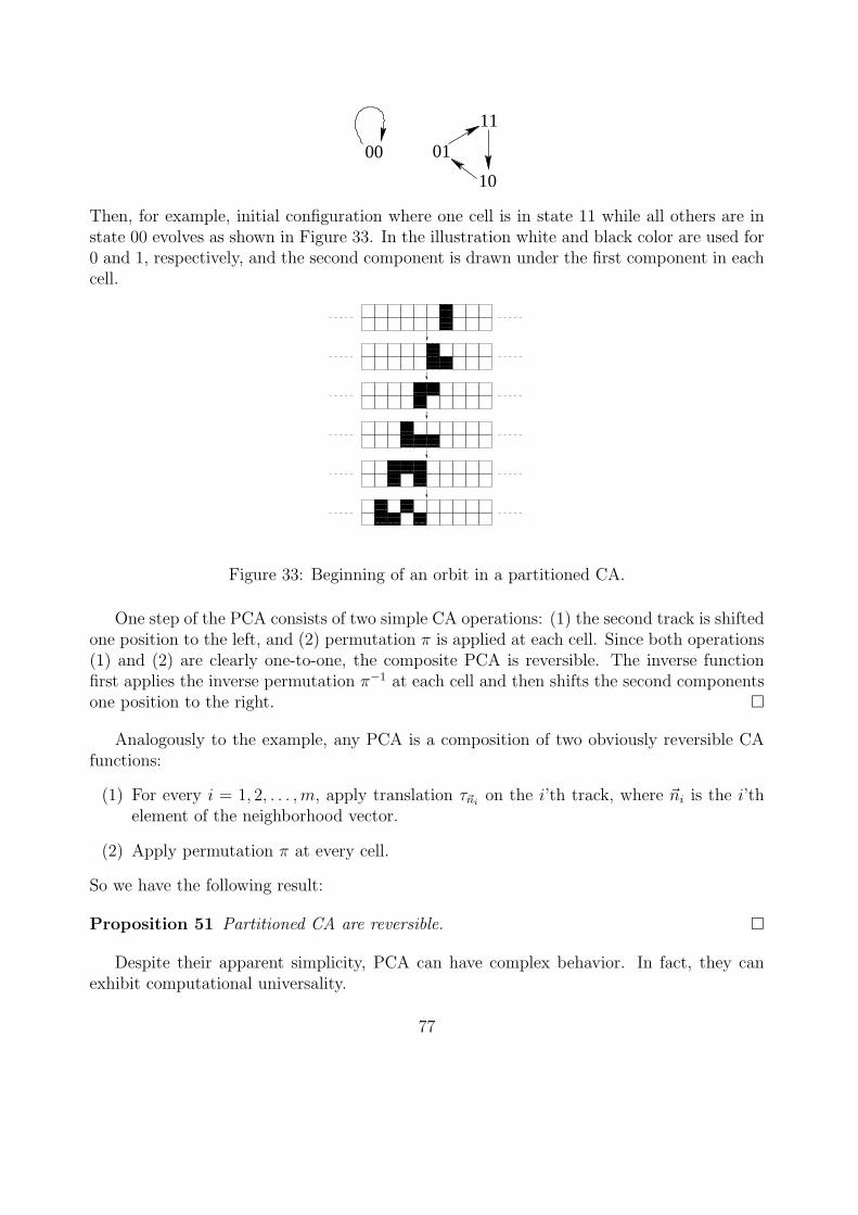
10

00 01

11

Then, for example, initial configuration where one cell is in state 11 while all others are instate 00 evolves as shown in Figure 33. In the illustration white and black color are used for0 and 1, respectively, and the second component is drawn under the first component in eachcell.

Figure 33: Beginning of an orbit in a partitioned CA.

One step of the PCA consists of two simple CA operations: (1) the second track is shiftedone position to the left, and (2) permutation π is applied at each cell. Since both operations(1) and (2) are clearly one-to-one, the composite PCA is reversible. The inverse functionfirst applies the inverse permutation π−1 at each cell and then shifts the second componentsone position to the right. ¤

Analogously to the example, any PCA is a composition of two obviously reversible CAfunctions:

(1) For every i = 1, 2, . . . , m, apply translation τ~nion the i’th track, where ~ni is the i’th

element of the neighborhood vector.

(2) Apply permutation π at every cell.

So we have the following result:

Proposition 51 Partitioned CA are reversible. ¤

Despite their apparent simplicity, PCA can have complex behavior. In fact, they canexhibit computational universality.

77

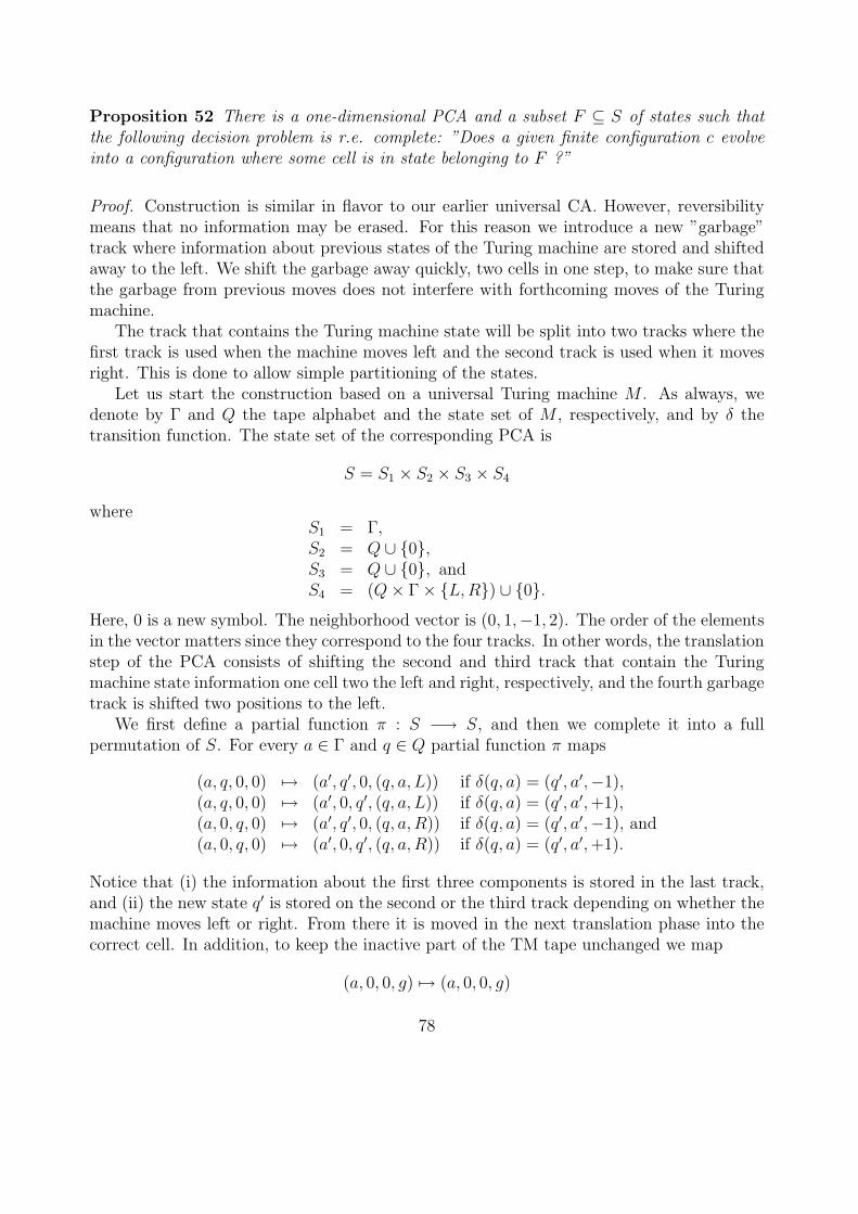
Proposition 52 There is a one-dimensional PCA and a subset F ⊆ S of states such thatthe following decision problem is r.e. complete: ”Does a given finite configuration c evolveinto a configuration where some cell is in state belonging to F ?”

Proof. Construction is similar in flavor to our earlier universal CA. However, reversibilitymeans that no information may be erased. For this reason we introduce a new ”garbage”track where information about previous states of the Turing machine are stored and shiftedaway to the left. We shift the garbage away quickly, two cells in one step, to make sure thatthe garbage from previous moves does not interfere with forthcoming moves of the Turingmachine.

The track that contains the Turing machine state will be split into two tracks where thefirst track is used when the machine moves left and the second track is used when it movesright. This is done to allow simple partitioning of the states.

Let us start the construction based on a universal Turing machine M . As always, wedenote by Γ and Q the tape alphabet and the state set of M , respectively, and by δ thetransition function. The state set of the corresponding PCA is

S = S1 × S2 × S3 × S4

whereS1 = Γ,S2 = Q ∪ 0,S3 = Q ∪ 0, andS4 = (Q× Γ× L, R) ∪ 0.

Here, 0 is a new symbol. The neighborhood vector is (0, 1,−1, 2). The order of the elementsin the vector matters since they correspond to the four tracks. In other words, the translationstep of the PCA consists of shifting the second and third track that contain the Turingmachine state information one cell two the left and right, respectively, and the fourth garbagetrack is shifted two positions to the left.

We first define a partial function π : S −→ S, and then we complete it into a fullpermutation of S. For every a ∈ Γ and q ∈ Q partial function π maps

(a, q, 0, 0) 7→ (a′, q′, 0, (q, a, L)) if δ(q, a) = (q′, a′,−1),(a, q, 0, 0) 7→ (a′, 0, q′, (q, a, L)) if δ(q, a) = (q′, a′, +1),(a, 0, q, 0) 7→ (a′, q′, 0, (q, a, R)) if δ(q, a) = (q′, a′,−1), and(a, 0, q, 0) 7→ (a′, 0, q′, (q, a, R)) if δ(q, a) = (q′, a′, +1).

Notice that (i) the information about the first three components is stored in the last track,and (ii) the new state q′ is stored on the second or the third track depending on whether themachine moves left or right. From there it is moved in the next translation phase into thecorrect cell. In addition, to keep the inactive part of the TM tape unchanged we map

(a, 0, 0, g) 7→ (a, 0, 0, g)

78

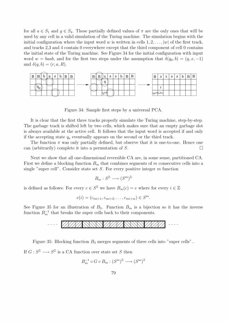
for all a ∈ S1 and g ∈ S4. These partially defined values of π are the only ones that will beused by any cell in a valid simulation of the Turing machine. The simulation begins with theinitial configuration where the input word w is written in cells 1, 2, . . . , |w| of the first track,and tracks 2,3 and 4 contain 0 everywhere except that the third component of cell 0 containsthe initial state of the Turing machine. See Figure 34 for the initial configuration with inputword w = baab, and for the first two steps under the assumption that δ(q0, b) = (q, x,−1)and δ(q, b) = (r, a, R).

q,B,L

a a bqx

q ,b,R0

B B B Bb a a b

q0

B B B B a a bxB B Ba

rq ,b,R0

Figure 34: Sample first steps by a universal PCA.

It is clear that the first three tracks properly simulate the Turing machine, step-by-step.The garbage track is shifted left by two cells, which makes sure that an empty garbage slotis always available at the active cell. It follows that the input word is accepted if and onlyif the accepting state qa eventually appears on the second or the third track.

The function π was only partially defined, but observe that it is one-to-one. Hence onecan (arbitrarily) complete it into a permutation of S. ¤

Next we show that all one-dimensional reversible CA are, in some sense, partitioned CA.First we define a blocking function Bm that combines segments of m consecutive cells into asingle ”super cell”. Consider state set S. For every positive integer m function

Bm : SZ −→ (Sm)Z

is defined as follows: For every c ∈ SZ we have Bm(c) = e where for every i ∈ Ze(i) = (cmi+1, cmi+2, . . . , cmi+m) ∈ Sm.

See Figure 35 for an illustration of B3. Function Bm is a bijection so it has the inversefunction B−1

m that breaks the super cells back to their components.

Figure 35: Blocking function B3 merges segments of three cells into ”super cells”..

If G : SZ −→ SZ is a CA function over state set S then

B−1m G Bm : (Sm)Z −→ (Sm)Z

79

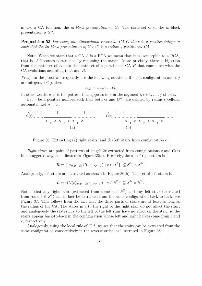
is also a CA function, the m-block presentation of G. The state set of of the m-blockpresentation is Sm.

Proposition 53 For every one-dimensional reversible CA G there is a positive integer nsuch that the 2n-block presentation of G σn is a radius-1

2partitioned CA.

Note: When we state that a CA A is a PCA we mean that it is isomorphic to a PCA,that is, A becomes partitioned by renaming the states. More precisely, there is bijectionfrom the state set of A onto the state set of a partitioned CA B that commutes with theCA evolutions according to A and B.

Proof. In the proof we frequently use the following notation: If c is a configuration and i, jare integers, i ≤ j, then

c[i,j] = cici+1 . . . cj.

In other words, c[i,j] is the pattern that appears in c in the segment i, i + 1, . . . , j of cells.Let r be a positive number such that both G and G−1 are defined by radius-r cellular

automata. Let n = 3r.

G(c)

r r r

cG(c)

r r r

c

(a) (b)

Figure 36: Extracting (a) right stairs, and (b) left stairs from configuration c.

Right stairs are pairs of patterns of length 2r extracted from configurations c and G(c)in a staggered way, as indicated in Figure 36(a). Precisely, the set of right stairs is

R = (c[0,2r−1], G(c)[−r,r−1]) | c ∈ SZ ⊆ S2r × S2r.

Analogously, left stairs are extracted as shown in Figure 36(b). The set of left stairs is

L = (G(c)[0,2r−1], c[−r,r−1]) | c ∈ SZ ⊆ S2r × S2r.

Notice that any right stair (extracted from some c ∈ SZ) and any left stair (extractedfrom some e ∈ SZ) can in fact be extracted from the same configuration back-to-back, seeFigure 37. This follows from the fact that the three parts of stairs are at least as long asthe radius of the CA. The states in c to the right of the right stair do not affect the stair,and analogously the states in e to the left of the left stair have no affect on the stair, so thestairs appear back-to-back in the configuration whose left and right halves come from c ande, respectively.

Analogously, using the local rule of G−1, we see that the stairs can be extracted from thesame configuration consecutively in the reverse order, as illustrated in Figure 38.

80

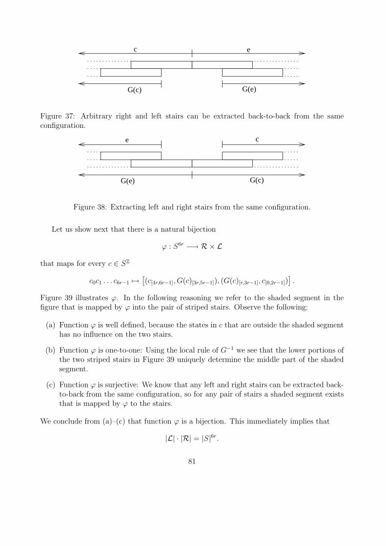
G(e)

c e

G(c)

Figure 37: Arbitrary right and left stairs can be extracted back-to-back from the sameconfiguration.

G(c)G(e)

e c

Figure 38: Extracting left and right stairs from the same configuration.

Let us show next that there is a natural bijection

ϕ : S6r −→ R×L

that maps for every c ∈ SZ

c0c1 . . . c6r−1 7→[(c[4r,6r−1], G(c)[3r,5r−1]), (G(c)[r,3r−1], c[0,2r−1])

].

Figure 39 illustrates ϕ. In the following reasoning we refer to the shaded segment in thefigure that is mapped by ϕ into the pair of striped stairs. Observe the following:

(a) Function ϕ is well defined, because the states in c that are outside the shaded segmenthas no influence on the two stairs.

(b) Function ϕ is one-to-one: Using the local rule of G−1 we see that the lower portions ofthe two striped stairs in Figure 39 uniquely determine the middle part of the shadedsegment.

(c) Function ϕ is surjective: We know that any left and right stairs can be extracted back-to-back from the same configuration, so for any pair of stairs a shaded segment existsthat is mapped by ϕ to the stairs.

We conclude from (a)–(c) that function ϕ is a bijection. This immediately implies that

|L| · |R| = |S|6r.

81

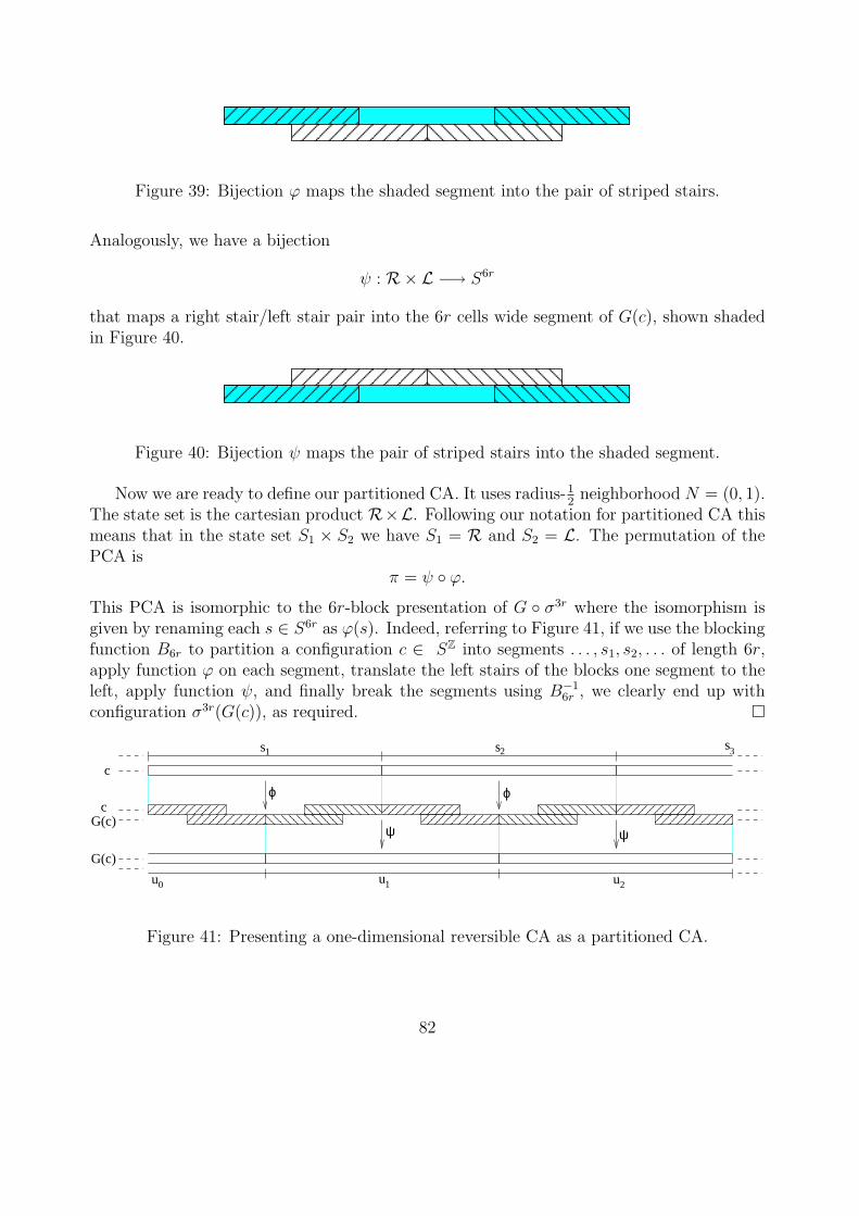
Figure 39: Bijection ϕ maps the shaded segment into the pair of striped stairs.

Analogously, we have a bijection

ψ : R×L −→ S6r

that maps a right stair/left stair pair into the 6r cells wide segment of G(c), shown shadedin Figure 40.

Figure 40: Bijection ψ maps the pair of striped stairs into the shaded segment.

Now we are ready to define our partitioned CA. It uses radius-12

neighborhood N = (0, 1).The state set is the cartesian product R×L. Following our notation for partitioned CA thismeans that in the state set S1 × S2 we have S1 = R and S2 = L. The permutation of thePCA is

π = ψ ϕ.

This PCA is isomorphic to the 6r-block presentation of G σ3r where the isomorphism isgiven by renaming each s ∈ S6r as ϕ(s). Indeed, referring to Figure 41, if we use the blockingfunction B6r to partition a configuration c ∈ SZ into segments . . . , s1, s2, . . . of length 6r,apply function ϕ on each segment, translate the left stairs of the blocks one segment to theleft, apply function ψ, and finally break the segments using B−1

6r , we clearly end up withconfiguration σ3r(G(c)), as required. ¤

ϕϕ

ψ ψ

u

s21

c

u21u0

G(c)

cG(c)

s s3

Figure 41: Presenting a one-dimensional reversible CA as a partitioned CA.

82

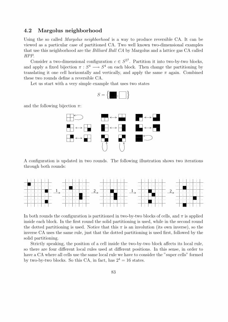
4.2 Margolus neighborhood

Using the so called Margolus neighborhood is a way to produce reversible CA. It can beviewed as a particular case of partitioned CA. Two well known two-dimensional examplesthat use this neighborhood are the Billiard Ball CA by Margolus and a lattice gas CA calledHPP.

Consider a two-dimensional configuration c ∈ SZ2. Partition it into two-by-two blocks,

and apply a fixed bijection π : S4 −→ S4 on each block. Then change the partitioning bytranslating it one cell horizontally and vertically, and apply the same π again. Combinedthese two rounds define a reversible CA.

Let us start with a very simple example that uses two states

S =

,

and the following bijection π:

A configuration is updated in two rounds. The following illustration shows two iterationsthrough both rounds:

2

1 2 1

In both rounds the configuration is partitioned in two-by-two blocks of cells, and π is appliedinside each block. In the first round the solid partitioning is used, while in the second roundthe dotted partitioning is used. Notice that this π is an involution (its own inverse), so theinverse CA uses the same rule, just that the dotted partitioning is used first, followed by thesolid partitioning.

Strictly speaking, the position of a cell inside the two-by-two block affects its local rule,so there are four different local rules used at different positions. In this sense, in order tohave a CA where all cells use the same local rule we have to consider the ”super cells” formedby two-by-two blocks. So this CA, in fact, has 24 = 16 states.

83

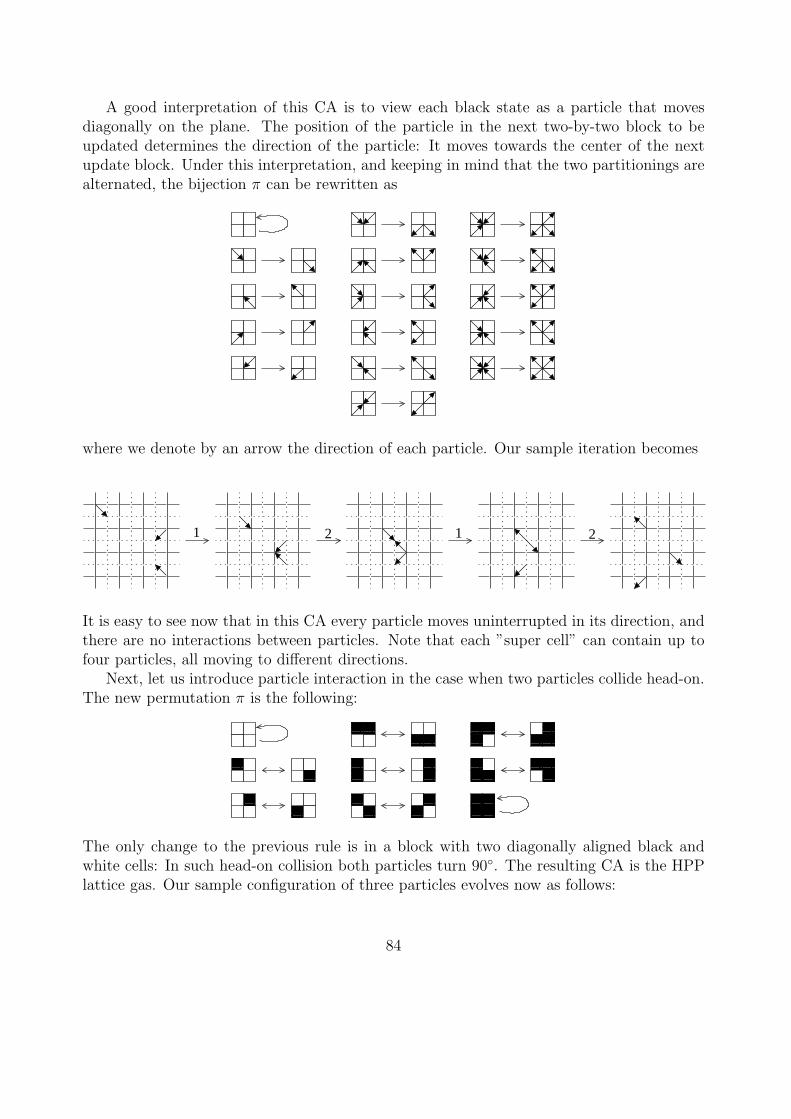
A good interpretation of this CA is to view each black state as a particle that movesdiagonally on the plane. The position of the particle in the next two-by-two block to beupdated determines the direction of the particle: It moves towards the center of the nextupdate block. Under this interpretation, and keeping in mind that the two partitionings arealternated, the bijection π can be rewritten as

where we denote by an arrow the direction of each particle. Our sample iteration becomes

21 2 1

It is easy to see now that in this CA every particle moves uninterrupted in its direction, andthere are no interactions between particles. Note that each ”super cell” can contain up tofour particles, all moving to different directions.

Next, let us introduce particle interaction in the case when two particles collide head-on.The new permutation π is the following:

The only change to the previous rule is in a block with two diagonally aligned black andwhite cells: In such head-on collision both particles turn 90. The resulting CA is the HPPlattice gas. Our sample configuration of three particles evolves now as follows:

84

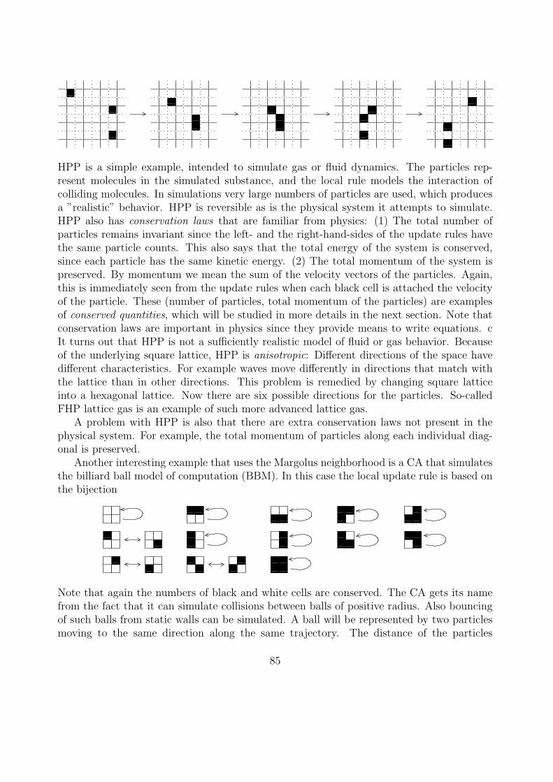
HPP is a simple example, intended to simulate gas or fluid dynamics. The particles rep-resent molecules in the simulated substance, and the local rule models the interaction ofcolliding molecules. In simulations very large numbers of particles are used, which producesa ”realistic” behavior. HPP is reversible as is the physical system it attempts to simulate.HPP also has conservation laws that are familiar from physics: (1) The total number ofparticles remains invariant since the left- and the right-hand-sides of the update rules havethe same particle counts. This also says that the total energy of the system is conserved,since each particle has the same kinetic energy. (2) The total momentum of the system ispreserved. By momentum we mean the sum of the velocity vectors of the particles. Again,this is immediately seen from the update rules when each black cell is attached the velocityof the particle. These (number of particles, total momentum of the particles) are examplesof conserved quantities, which will be studied in more details in the next section. Note thatconservation laws are important in physics since they provide means to write equations. cIt turns out that HPP is not a sufficiently realistic model of fluid or gas behavior. Becauseof the underlying square lattice, HPP is anisotropic: Different directions of the space havedifferent characteristics. For example waves move differently in directions that match withthe lattice than in other directions. This problem is remedied by changing square latticeinto a hexagonal lattice. Now there are six possible directions for the particles. So-calledFHP lattice gas is an example of such more advanced lattice gas.

A problem with HPP is also that there are extra conservation laws not present in thephysical system. For example, the total momentum of particles along each individual diag-onal is preserved.

Another interesting example that uses the Margolus neighborhood is a CA that simulatesthe billiard ball model of computation (BBM). In this case the local update rule is based onthe bijection

Note that again the numbers of black and white cells are conserved. The CA gets its namefrom the fact that it can simulate collisions between balls of positive radius. Also bouncingof such balls from static walls can be simulated. A ball will be represented by two particlesmoving to the same direction along the same trajectory. The distance of the particles

85

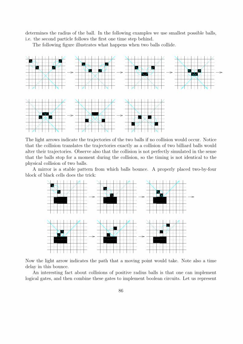
determines the radius of the ball. In the following examples we use smallest possible balls,i.e. the second particle follows the first one time step behind.

The following figure illustrates what happens when two balls collide.

The light arrows indicate the trajectories of the two balls if no collision would occur. Noticethat the collision translates the trajectories exactly as a collision of two billiard balls wouldalter their trajectories. Observe also that the collision is not perfectly simulated in the sensethat the balls stop for a moment during the collision, so the timing is not identical to thephysical collision of two balls.

A mirror is a stable pattern from which balls bounce. A properly placed two-by-fourblock of black cells does the trick:

Now the light arrow indicates the path that a moving point would take. Note also a timedelay in this bounce.

An interesting fact about collisions of positive radius balls is that one can implementlogical gates, and then combine these gates to implement boolean circuits. Let us represent

86

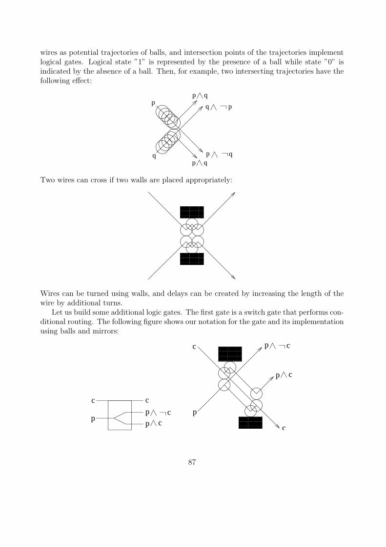
wires as potential trajectories of balls, and intersection points of the trajectories implementlogical gates. Logical state ”1” is represented by the presence of a ball while state ”0” isindicated by the absence of a ball. Then, for example, two intersecting trajectories have thefollowing effect:

p

p q

p qp

q p q

q

Two wires can cross if two walls are placed appropriately:

Wires can be turned using walls, and delays can be created by increasing the length of thewire by additional turns.

Let us build some additional logic gates. The first gate is a switch gate that performs con-ditional routing. The following figure shows our notation for the gate and its implementationusing balls and mirrors:

c

c c

pp

pc

p c

p cc

p

c

87

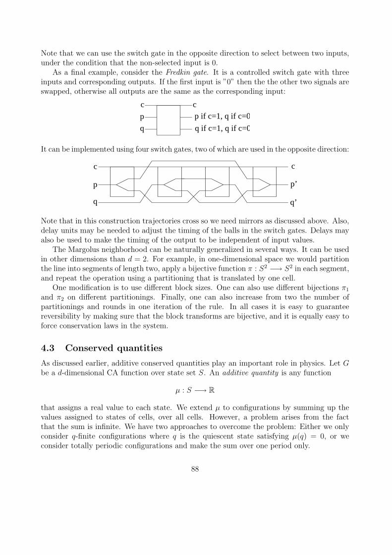
Note that we can use the switch gate in the opposite direction to select between two inputs,under the condition that the non-selected input is 0.

As a final example, consider the Fredkin gate. It is a controlled switch gate with threeinputs and corresponding outputs. If the first input is ”0” then the the other two signals areswapped, otherwise all outputs are the same as the corresponding input:

p if c=1, q if c=0c c

p

q q if c=1, q if c=0

It can be implemented using four switch gates, two of which are used in the opposite direction:

q

c

p

c

p’

q’

Note that in this construction trajectories cross so we need mirrors as discussed above. Also,delay units may be needed to adjust the timing of the balls in the switch gates. Delays mayalso be used to make the timing of the output to be independent of input values.

The Margolus neighborhood can be naturally generalized in several ways. It can be usedin other dimensions than d = 2. For example, in one-dimensional space we would partitionthe line into segments of length two, apply a bijective function π : S2 −→ S2 in each segment,and repeat the operation using a partitioning that is translated by one cell.

One modification is to use different block sizes. One can also use different bijections π1

and π2 on different partitionings. Finally, one can also increase from two the number ofpartitionings and rounds in one iteration of the rule. In all cases it is easy to guaranteereversibility by making sure that the block transforms are bijective, and it is equally easy toforce conservation laws in the system.

4.3 Conserved quantities

As discussed earlier, additive conserved quantities play an important role in physics. Let Gbe a d-dimensional CA function over state set S. An additive quantity is any function

µ : S −→ R

that assigns a real value to each state. We extend µ to configurations by summing up thevalues assigned to states of cells, over all cells. However, a problem arises from the factthat the sum is infinite. We have two approaches to overcome the problem: Either we onlyconsider q-finite configurations where q is the quiescent state satisfying µ(q) = 0, or weconsider totally periodic configurations and make the sum over one period only.

88

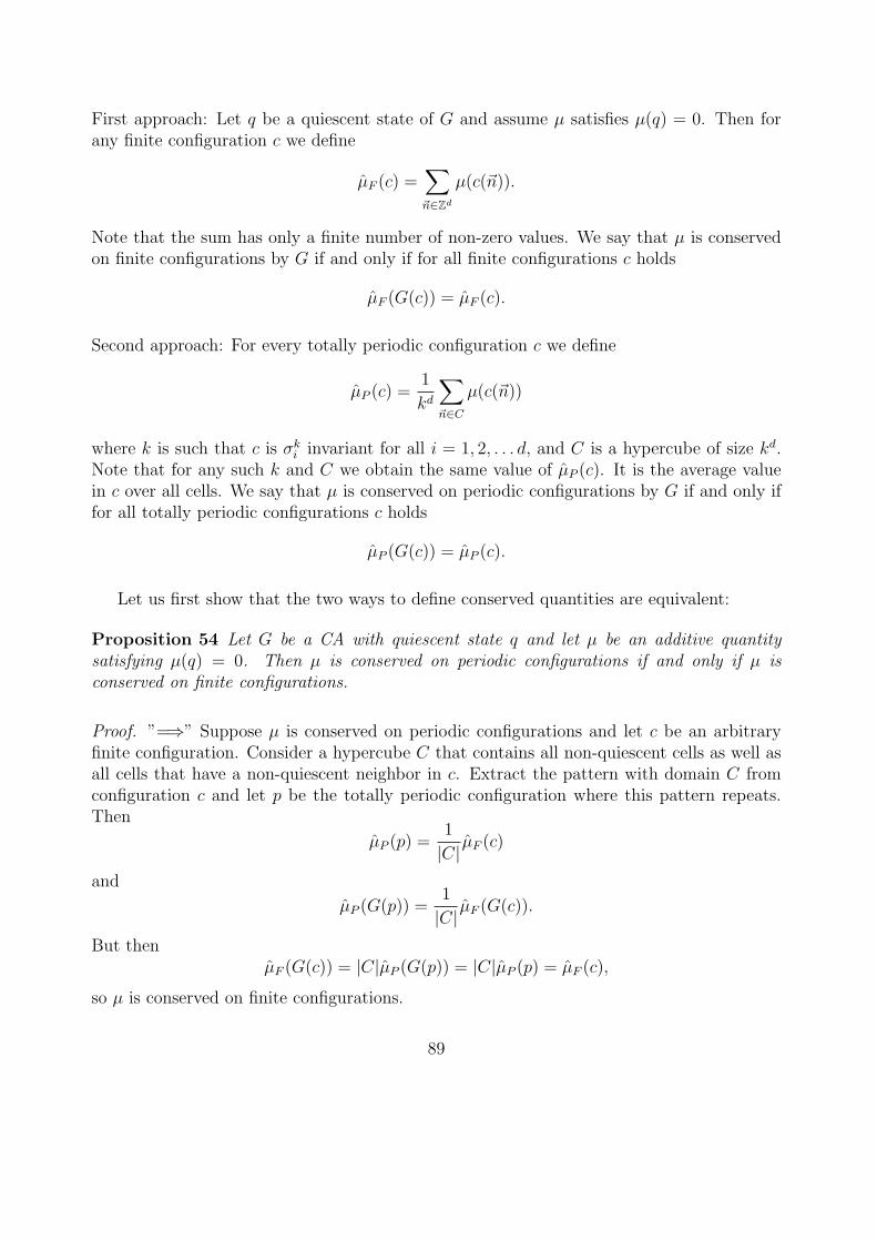
First approach: Let q be a quiescent state of G and assume µ satisfies µ(q) = 0. Then forany finite configuration c we define

µF (c) =∑

~n∈Zd

µ(c(~n)).

Note that the sum has only a finite number of non-zero values. We say that µ is conservedon finite configurations by G if and only if for all finite configurations c holds

µF (G(c)) = µF (c).

Second approach: For every totally periodic configuration c we define

µP (c) =1

kd

∑

~n∈C

µ(c(~n))

where k is such that c is σki invariant for all i = 1, 2, . . . d, and C is a hypercube of size kd.

Note that for any such k and C we obtain the same value of µP (c). It is the average valuein c over all cells. We say that µ is conserved on periodic configurations by G if and only iffor all totally periodic configurations c holds

µP (G(c)) = µP (c).

Let us first show that the two ways to define conserved quantities are equivalent:

Proposition 54 Let G be a CA with quiescent state q and let µ be an additive quantitysatisfying µ(q) = 0. Then µ is conserved on periodic configurations if and only if µ isconserved on finite configurations.

Proof. ”=⇒” Suppose µ is conserved on periodic configurations and let c be an arbitraryfinite configuration. Consider a hypercube C that contains all non-quiescent cells as well asall cells that have a non-quiescent neighbor in c. Extract the pattern with domain C fromconfiguration c and let p be the totally periodic configuration where this pattern repeats.Then

µP (p) =1

|C| µF (c)

and

µP (G(p)) =1

|C| µF (G(c)).

But thenµF (G(c)) = |C|µP (G(p)) = |C|µP (p) = µF (c),

so µ is conserved on finite configurations.

89

”⇐=” Suppose µ is conserved on finite configurations and let p be an arbitrary totallyperiodic configuration. Let C be a hypercube of size kd where k is such that p is invariantunder translations σk

i for all i = 1, 2, . . . , d. We may also assume that k is larger than theradius of the CA that defines G. Let j be a large positive integer, and construct a finiteconfiguration c that consists of a size (jk)d hypercube extracted from p, with copies of thequiescent state q outside the hypercube. Then

µF (c) = (jk)dµP (p).

Configurations G(c) and G(p) agree inside a size (jk− 2k)d hypercube, and in G(c) all cellsoutside the co-centric size (jk + 2k)d hypercube are quiescent. Let

m = max|µ(s)| | s ∈ S

be the maximum absolute value assigned to any state. We have

∣∣µF (G(c))− (jk)dµP (G(p))∣∣ ≤ 2m

[(jk + 2k)d − (jk − 2k)d

] ≤ 2m[4dk(jk + 2k)d−1

].

Because µ is conserved on finite configurations,

µF (G(c)) = µF (c) = (jk)dµP (p),

so we have

|µP (p)− µP (G(p))| ≤ 8dkm(jk + 2k)d−1

(jk)d−→ 0

when j −→∞. This means that

µP (p) = µP (G(p)).

¤

Note that the restriction that µ(q) = 0 is not important: if µ is conserved on periodicconfigurations so is µ′ where µ′(s) = µ(s) + c for some constant c. So if µ(q) 6= 0 we canconsider µ′(s) = µ(s)− µ(q) instead. It satisfies the constraint µ′(q) = 0 and it is conservedon periodic configurations if and only if µ is.

Since the two concepts of conservation are equivalent we concentrate on finite configura-tions in the following. From now on we denote briefly µ for µF , and say that the quantity isconserved if it is conserved on finite configurations.

The following proposition provides an efficient characterization for conserved quantities.

Proposition 55 Quantity µ is conserved if and only if for any two finite configurations c1

and c2 that differ in a single cell holds

µ(c1)− µ(c2) = µ(G(c1))− µ(G(c2)). (8)

90

Proof. If µ is conserved then µ(G(c1)) = µ(c1) and µ(G(c2)) = µ(c2) so the given equationholds. Conversely, suppose the given equation holds, and let c be an arbitrary finite config-uration. Then there exists a finite sequence of configurations c1, c2, . . . , cn where c1 is thequiescent configuration, cn = c, and configurations ci and ci+1 differ in a single cell for alli = 1, 2, . . . , n− 1. By the hypothesis we have

µ(ci)− µ(ci+1) = µ(G(ci))− µ(G(ci+1))

for all i = 1, 2, . . . , n− 1. Adding all these equations together gives

µ(c1)− µ(cn) = µ(G(c1))− µ(G(cn))

Since G(c1) = c1 and cn = c, we obtain

µ(G(c)) = µ(c).

¤

Let us look at equations (8) in detail. Since µ is translation invariant, it is sufficient toconsider only configurations c1 and c2 that differ in cell ~0 and agree at all other cells. In thedifference on the left-hand-side of (8) most values cancel out, so in fact

µ(c1)− µ(c2) = µ(c1(~0))− µ(c2(~0)).

Analogously, since G(c1) and G(c2) agree on all cells but those that have ~0 in their neigh-borhood, the right-hand-side of (8) becomes

µ(G(c1))− µ(G(c2)) =∑

~n∈A

µ(G(c1)(~n))− µ(G(c2)(~n))

whereA = −~ni | i = 1, 2, . . . , m

is the set of all cells that have ~0 as a neighbor. From this we already see the interesting factthat there are only a finite number of different equations (8).

Let c1 and c2 be two finite configurations that only differ in cell ~0, let c′1 and c′2 be anothersuch pair, and suppose that c1 and c′1 agree with each other inside region

B = ~nj − ~ni | i, j = 1, 2, . . . , m,

and suppose that c2 and c′2 also agree inside B. Notice that region B contains all cells thatare neighbors of elements of A, so G(c1) and G(c′1) agree in A, and also G(c2) and G(c′2) agreein A. Then the equation (8) we obtain using c1 and c2 is the same as the equation that weobtain if we use c′1 and c′2 instead. This means that it is enough to form the equations (8) fordifferent patterns with domain B. In other words, for all pairs p1 = (B, g1) and p2 = (B, g2)

91

of patterns with domain B, where g1(~n) = g2(~n) for all ~n 6= ~0 and g1(~0) 6= g2(~0), we calculatethe successors (A, h1) = G(p1) and (A, h2) = G(p2), and form the corresponding equation

µ(g1(~0))− µ(g2(~0)) =∑

~n∈A

µ(h1(~n))− µ(h2(~n)).

Quantity µ is conserved by G if and only if it satisfies all these equations. In addition,requirement µ(q) = 0 may be added where q is the quiescent state, although this is notnecessary since µ(q) = 0 only scales the quantity by an additive constant.

If the CA has no quiescent state q we may pick an arbitrary ground state q and considerq-finite configurations. The considerations above work unaltered, but we have to add theequation

µ(q) = µ(f(q, q, . . . , q))

stating that the quantity is conserved on the configuration where all cells are in state q.In fact, we can reduce the number of equations further by a more careful inspection of the

proof of Proposition 55. For simplicity, let us consider one-dimensional CA only (although asimilar analysis works for higher dimensional cases as well). The quiescent configuration canbe transformed into any desired finite configuration by changing states of cells one-by-one inthe left-to-right order. This means that configurations c1 and c2 in the equation (8) satisfythe additional constraint that all cells to the right of the position where c1 and c2 differ arequiescent. This means that it is enough to form equations using patterns p1 = (B, g1) andp2 = (B, g2) that satisfy the following constraints (in the one-dimensional case):

• g1(n) = g2(n) = q for all n > 0,

• g1(0) = q and g2(0) 6= q, and

• g1(n) = g2(n) for all n < 0.

Example 26. As an example, let us find conservation laws of the traffic CA, that is, theelementary CA with Wolfram number 226. The local rule replaces pattern 01 by pattern 10:

000 7→ 0 001 7→ 1 010 7→ 0 011 7→ 0100 7→ 0 101 7→ 1 110 7→ 1 111 7→ 1

The neighborhood vector is N = (−1, 0, 1), so A = −1, 0, 1 and B = −2,−1, 0, 1, 2. Thismeans that changing the state of cell 0 may affect the states of cells -1,0 and 1, and howthese are affected depends on the old states of cells in the set B. It is hence sufficient to formthe equations based on patterns with domain B. As discussed above, it is in fact sufficientto form equations (8) based on pairs of patterns ab000 and ab100 for all a, b ∈ 0, 1.

For a = 0, b = 0 we obtain from

0 0 0 0 0 0 0 1 0 00 0 0 1 0 0

92

the equationµ(0)− µ(1) = 3µ(0)− [µ(1) + 2µ(0)].

This yields the trivial relation 0 = 0. For a = 0, b = 1 we get from

0 1 0 0 0 0 1 1 0 00 0 0 0 1 0

also the trivial equation 0 = 0. For a = 1, b = 0 we have

1 0 0 0 0 1 0 1 0 00 0 0 1 0 0

which is again trivial, and finally, for a = b = 1 we have

1 1 0 0 0 1 1 1 0 01 0 0 1 1 0

which also yields the trivial equation. We conclude that in traffic CA all functions µ areconserved. In particular, number of cells in state 1 is conserved. ¤

Example 27. Consider the CA discussed in Example 11. It uses the radius-12

neighborhoodN = (0, 1), so A = −1, 0 and B = −1, 0, 1. The state set is S = 0, 1, 2 and the localrule f is

f(a, b) =

2, if a = 2,0, if a 6= 2 and a + b is even, and1, if a 6= 2 and a + b is odd.

Now it is enough to consider pairs of patterns a00 and ab0 for a, b ∈ S, b 6= 0.

0 0 0 0 1 00 0 1 1

=⇒ µ(0)− µ(1) = 2µ(0)− 2µ(1) =⇒ µ(0) = µ(1)

0 0 0 0 2 00 0 0 2

=⇒ µ(0)− µ(2) = 2µ(0)− µ(0)− µ(2) =⇒ 0 = 0

1 0 0 1 1 01 0 0 1

=⇒ µ(0) = µ(1)

1 0 0 1 2 01 0 1 2

=⇒ 0 = 0

2 0 0 2 1 02 0 2 1

=⇒ 0 = 0

2 0 0 2 2 02 0 2 2

=⇒ 0 = 0

93

We conclude that any µ satisfying µ(0) = µ(1) is conserved. In particular, the number of2’s is conserved.

¤

As a final note, we observe that for any fixed CA, the additive quantities that it conservesform a linear space, when sum and scalar product are defined in the natural way, point wise:

(µ + µ′)(a) = µ(a) + µ′(a) for all µ, µ′ ∈ RS and a ∈ S,(rµ)(a) = rµ(a) for all µ ∈ RS, r ∈ R and a ∈ S.

If G conserves µ and µ′ then for any q-finite configuration c and every r ∈ R holds

(µ + µ′)(c) = µ(c) + µ′(c) = µ(G(c)) + µ′(G(c)) = (µ + µ′)(G(c))

and(rµ)(c) = rµ(c) = r(µ(G(c)) = (rµ)(G(c)),

which proves the linearity of the conserved quantities of G. Note also that equations (8) arelinear, so we have an algorithm to build a system of linear equations whose solutions areexactly the conserved quantities of G.

5 Cellular automata dynamical systems

An especially fruitful view to cellular automata dynamics is to endow the configuration spaceSZ

dwith a metric under which CA functions G are continuous. This makes the tools and

results of topological dynamics available to the analysis of cellular automata. The space SZd

under this metric is compact and complete. Convergence of a sequence c1, c2, . . . of elementsunder this metric is exactly equivalent to the convergence introduced in Section 1.8. Thecompactness principle (Proposition 4) of that section then simply states the compactness ofthe metric space.

First, for any ~x ∈ Zd we denote

‖(x1, x2 . . . , xd)‖ = max|x1|, |x2|, . . . , |xd|.See Figure 42 for an illustration in the two dimensional case. Then, we define the distanced(e, c) between configurations e, c ∈ SZ

das follows:

d(e, c) =

0, if e = c,2−min ‖~x‖ | c(~x)6=e(~x), if e 6= c.

In other words, two configurations that differ in a cell that is close to ~0 are far away fromeach other under this metric, while configurations that agree with each other on a largearea around the origin are close to each other. Under this metric, two configurations havedistance < 2−r if and only if they agree with each other at all positions (x, y) where ‖~x‖ ≤ r.

Note that other vector norms ‖·‖ could be used as well, and any other decreasing functionwhose limit at ∞ is 0 could be used instead of x 7→ 2−x. A different metric, but the sametopology would result.

94

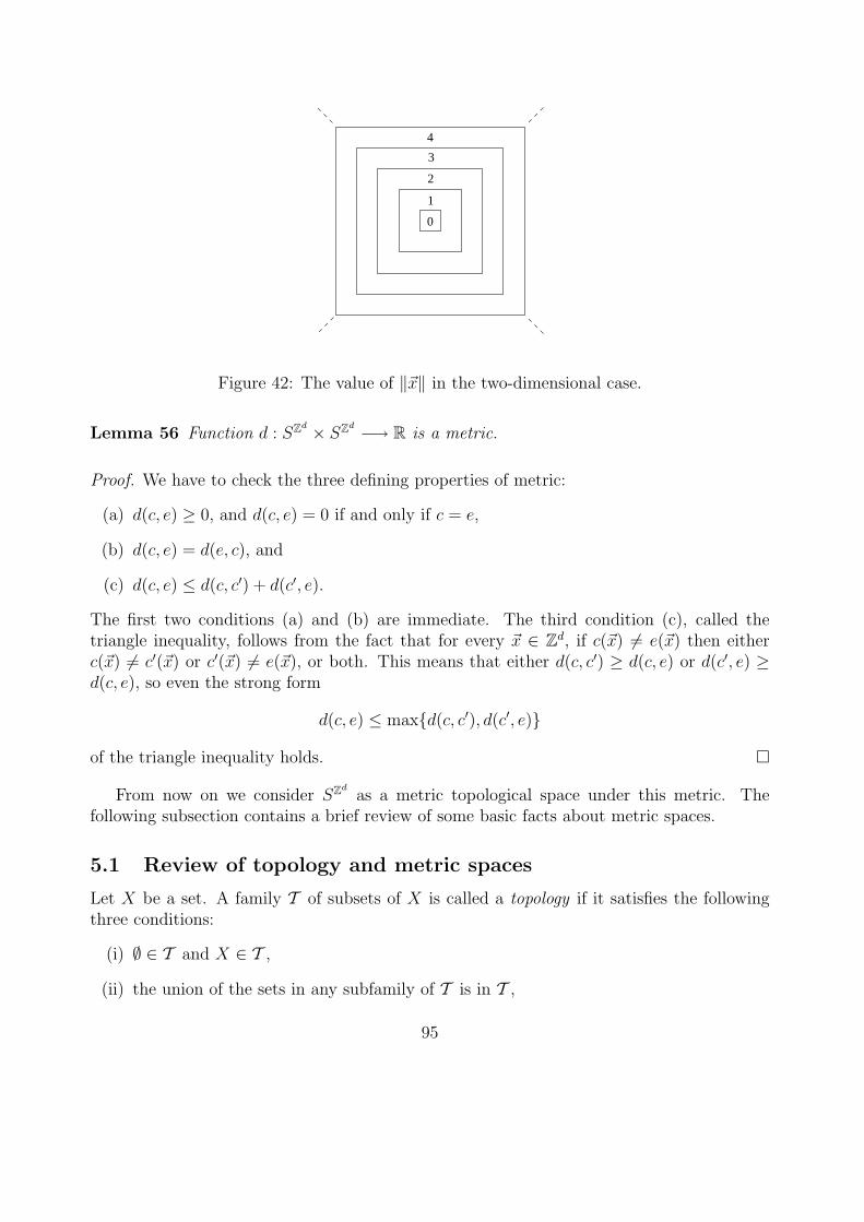
4

0

3

2

1

Figure 42: The value of ‖~x‖ in the two-dimensional case.

Lemma 56 Function d : SZd × SZ

d −→ R is a metric.

Proof. We have to check the three defining properties of metric:

(a) d(c, e) ≥ 0, and d(c, e) = 0 if and only if c = e,

(b) d(c, e) = d(e, c), and

(c) d(c, e) ≤ d(c, c′) + d(c′, e).

The first two conditions (a) and (b) are immediate. The third condition (c), called thetriangle inequality, follows from the fact that for every ~x ∈ Zd, if c(~x) 6= e(~x) then eitherc(~x) 6= c′(~x) or c′(~x) 6= e(~x), or both. This means that either d(c, c′) ≥ d(c, e) or d(c′, e) ≥d(c, e), so even the strong form

d(c, e) ≤ maxd(c, c′), d(c′, e)

of the triangle inequality holds. ¤

From now on we consider SZd

as a metric topological space under this metric. Thefollowing subsection contains a brief review of some basic facts about metric spaces.

5.1 Review of topology and metric spaces

Let X be a set. A family T of subsets of X is called a topology if it satisfies the followingthree conditions:

(i) ∅ ∈ T and X ∈ T ,

(ii) the union of the sets in any subfamily of T is in T ,

95

(iii) the intersection of finitely many elements of T is always in T .

Elements of T are called open sets, and their complements (with respect to X) are closedsets. A set that is both open and closed is called clopen.

Example 28. For any X, let T contain all subsets of X. Then T is a topology, the discretetopology of X. Also X, ∅ is a topology, the trivial topology of X. ¤

Example 29. Let us call S ⊆ R open if for every x ∈ S there is a positive real ε > 0 suchthat |y − x| < ε =⇒ y ∈ S. These open sets form a topology of X = R. It is called theusual topology of R. For example, all open intervals (a, b) for a < b are open sets. Closedintervals [a, b] are not open but they are closed. Set Q of rational numbers is not open orclosed. The only clopen sets are ∅ and R. ¤

Generalizing the previous example, let X be a set and let d : X ×X −→ R be a metric.For every ε > 0 and x ∈ X we denote

Bε(x) = y ∈ X | d(x, y) < ε

and call Bε(x) the (open) ε-ball with center x. Let us call U ⊆ X open if

∀x ∈ U : ∃ε > 0 : Bε(x) ⊆ U.

These open sets form a topology of X, the metric topology induced by d.

Example 30. The discrete topology is induced by the discrete metric

d(x, y) =

0, if x = y,1, if x 6= y.

In contrast, if |X| ≥ 2 then the trivial topology X, ∅ is not metric. ¤

Let A ⊆ X. Point x ∈ X is an accumulation point of A if every open set U that containsx also contains some element y 6= x of A. The following simple properties hold for closedsets:

Proposition 57 A subset A ⊆ X is closed if and only if its accumulation points belongto A. Closed sets satisfy the following properties (that are dual statements of the definingproperties of open sets):

(i) The empty set ∅ is closed, and X is closed,

(ii) the intersection of any number of closed sets is closed, and

(iii) the union of a finite number of closed sets is closed.

¤

96

Let A ⊆ X. The closure of A is the intersection of all closed sets that contain A. It isthen the smallest closed set that contains A. We denote the closure of A by A. Notice thatA itself is closed if and only if A = A. Notice also that the closure of A is the union of Aand its set of accumulation points.

Set A is called dense if A = X.

Example 31. Consider the usual topology of R. All real numbers are accumulation pointsof the set Q of rational numbers. This means that the closure of Q is R, so Q is dense in R.Accumulation points of the open interval (0, 1) are the elements of the closed interval [0, 1],while the set Z of integers has no accumulation points. ¤

Let A ⊆ X. Point x ∈ A is an interior point of A if there is an open set U such thatx ∈ U and U ⊆ A. The set A of all interior points of A is the interior of A. It is easilyseen to be the union of all open subsets of A, or equivalently, the largest open subset of A.Then set A is open if and only if its interior is A itself.

The exterior of set A ⊆ X is the interior of the complement of A, and the boundary of Aconsists of all points that are not in the interior or the exterior of A. Note that the interior,exterior and boundary of A is a partitioning of X. A set A ⊆ X is called a neighborhood ofx ∈ X if x is an interior point of A, that is, if there is an open set U such that x ∈ U ⊆ A.

Example 32. In the usual topology of R, the interior, exterior and the boundary of an openinterval (a, b) are (a, b), (−∞, a) ∪ (b,∞) and a, b, respectively. The closed interval [a, b]has these same interior, exterior and boundary. Set Q has empty interior and exterior. Allreal numbers are in its boundary. ¤

A topology is called Hausdorff if for every x 6= y there are open Ux and Uy such thatx ∈ Ux, y ∈ Uy and Ux∩Uy = ∅. In other words, any two distinct points have non-intersectingneighborhoods.

Example 33. Every metric topology is Hausdorff. Indeed, if x 6= y then d(x, y) > 0. If wechoose ε = 1

2d(x, y) then Bε(x) and Bε(y) are non-intersecting neighborhoods of x and y ¤

A sequence x1, x2, . . . of points of X converges to point x ∈ X if for every open U ⊆ Xthat contains x there is positive integer n such that xi ∈ U for all i ≥ n. If the topology ismetric this is equivalent to saying that for every ε > 0 there is n such that d(xi, x) < ε forall i ≥ n.

Note that generally a converging sequence may converge to several different points, butif the topology is Hausdorff (e.g. metric) the limit is unique.

Proposition 58 In Hausdorff topology every converging sequence converges to a uniquepoint. ¤

Proof. Suppose x1, x2, . . . converges to x and y where x 6= y. Since X is Hausdorff, there areopen sets U and V such that x ∈ U , y ∈ V and U ∩V = ∅. By the definition of convergence,xi ∈ U and xi ∈ V for all sufficiently large i, a contradiction. ¤

97

Note: the proposition does not hold in all topological spaces. For example, in the trivialtopology T = ∅, X every sequence converges to every point.

In Hausdorff topology we denote by limi→∞ xi the unique point into which the sequencex1, x2, . . . converges, if it exists. This point is the limit of the sequence.

The following proposition states that if the topology is metric then the closure A of anyset A consists exactly of the limits of converging sequences of elements of A:

Proposition 59 Let X be a metric space and A ⊆ X. Then x ∈ A if and only if x =limi→∞ ai for some converging sequence a1, a2, . . . where all ai ∈ A.

Proof. ”⇐=”: Let a1, a2, . . . be a converging sequence where all ai ∈ A and let x = limi→∞ ai.Let U be an arbitrary open set that contains x. By the definition of convergence there aresome ai ∈ U , so U ∩ A 6= ∅. This means that x ∈ A. (This direction of the proof holds forany topological space.)

”=⇒”: Conversely, suppose x ∈ A. For every positive integer i, let ai be an element ofA ∩B 1

i(x). Then d(x, ai) < 1

i, so x = limi−→∞ ai. ¤

Corollary 60 In metric space X, set A is closed if and only if it contains the limit of everyconverging sequence of its elements. ¤

A family B of open sets is called a base of the topology iff every open set is the union ofsome members of B. Equivalently: B ⊆ T is a base if for every open set U and x ∈ U thereexists some B ∈ B with the property that x ∈ B ⊆ U .

Example 34. The open intervals (a, b) with a < b form a base of the usual topology of R.More generally, in any metric topology the open balls Bε(x) over all ε > 0 and x ∈ X forma base. ¤

If B is a base of a topology then this topology is uniquely determined by B: open setsare exactly the unions of members of B. The following proposition gives a necessary andsufficient condition on when a family B is a base of some topology:

Proposition 61 B is a base of a topology if and only if it satisfies the following two condi-tions:

(i) Every x ∈ X belongs to some B ∈ B, and

(ii) For every A,B ∈ B and every x ∈ A ∩B there is C ∈ B such that x ∈ C ⊆ A ∩B.

Proof. Suppose first that B is a base of a topology. Condition (i) follows from the fact thatX is open. Let us prove (ii). Let A,B ∈ B be arbitrary, and let x ∈ A ∩ B. Because A andB are both open, so is A∩B. Hence there is a base set C ∈ B that satisfies x ∈ C ⊆ A∩B.

98

Conversely, suppose (i) and (ii) hold, and let T contain all unions of all subfamilies of B.The empty union is ∅ so ∅ ∈ T . It follows from (i) that the union of all elements in B is X,so X ∈ T .

Let Ui be arbitrary elements of T . Then each Ui is a union of elements of B, so theirunion is also a union of elements of B. Hence the union of Ui’s is in T .

Consider then arbitrary U, V ∈ T , and let x ∈ U ∩V . Because x ∈ U , and U is a union ofmembers of B, there is some A ∈ B such that x ∈ A ⊆ U . Analogously there is some B ∈ Bsuch that x ∈ B ⊆ V . By property (ii) there is C ∈ B such that x ∈ C ⊆ A ∩ B ⊆ U ∩ V .Such C exists for every x, so we see that U ∩ V ∈ T . This means that the intersection offinitely many elements of T is in T . ¤

Next we define compactness. Let A ⊆ X where X is a topological space. A familyof open sets Ui is called an open cover of A if every element of A belongs to some Ui. Asubfamily of an open cover of A is called a subcover if it is also a cover of A.

Set A ⊆ X is called compact if every open cover of A has a finite subcover of A. Thetopology is called compact if the whole space X is compact. In other words, a topology iscompact if every family of open sets whose union is X has a finite subfamily whose union isX.

Example 35. In the usual topology of R the set

A = 0 ∪ 1

n| n ∈ Z+

is compact. Namely, an open set that contains 0 covers all but finitely many elements of A.So any open cover of A contains a finite subcover: Open set U that covers 0 together with afinite number of open sets that cover the finitely many elements of A that are outside of U .

On the other hand, set B = 1n| n ∈ Z+ is not compact. It has an open cover in which

every open set covers exactly one element of B. Such cover has no finite subcover. ¤

The following proposition states the finite intersection property. It is dual to the opencover property we used as the definition, and in fact the finite intersection property couldhave been taken equally well as the definition of compactness. We state the property for thewhole space X:

Proposition 62 Topology of X is compact if and only if every family of closed sets whoseintersection is empty has a finite subfamily whose intersection is empty.

Proof. This follows directly from the definition of compactness and de Morgan’s laws: Afamily of open sets is a cover of X if and only if the family of their complements have emptyintersection. ¤

We typically apply the previous proposition in the following set-up:

99

Corollary 63 Let F1 ⊇ F2 ⊇ F3 ⊇ . . . be an infinite chain of closed sets in a compact spaceX. If

∞⋂i=1

Fi = ∅,

then Fi = ∅ for some i. ¤

The next proposition gives a characterization of compact subsets in metric spaces. Theproposition gives a condition that looks very similar to Proposition 4 for configurations. Infact, we use the proposition later to show the compactness of the configuration space. Theproposition is valid (and is stated) for arbitrary metric spaces, but we only prove it now formetric spaces that have a countable base. Our configuration space satisfies this restriction,so the proof is sufficient for our set-up. The proof for general metric spaces is not verydifficult either.

Proposition 64 Suppose X is a metric space. Set A ⊆ X is compact if and only if everysequence a1, a2, . . . of elements of A has a subsequence that converges to an element of A.

Proof. ”=⇒” Suppose A is compact, and let a1, a2, . . . be arbitrary sequence where eachai ∈ A.

Suppose first that there is some a ∈ A such that for every ε > 0 the ball Bε(a) containsinfinitely many different elements of the sequence a1, a2, . . .. Then the sequence has a sub-sequence that converges to a: There namely is a subsequence whose n’th element belongs toB 1

n(a).

Suppose then that for every a ∈ A there is some εa > 0 such that Bεa(a) only containsfinitely many different elements of the sequence a1, a2, . . .. Clearly the family of Bεa(a) overall a ∈ A is an open cover of A, so by compactness of A it has a finite subcover

Ui = Bεai(ai) for i = 1, 2, . . . m.

But each Ui only covers finitely many different elements of sequence a1, a2, . . ., while eachelement of the sequence is covered by some Ui. This means that the sequence has onlyfinitely many different elements. Then some element a ∈ A repeats infinitely many times inthe sequence so the sequence has a constant subsequence a, a, . . . which trivially convergesto a ∈ A.

”⇐=” Suppose every sequence of elements of A has a converging subsequence whose limit isin A. Here we simplify the set-up by making the additional assumption that the topologyhas a countable base. Then it is enough to show that any countable open cover of A hasa finite sub-cover. (Indeed, for an arbitrary open cover by Ui we can consider instead thecountable cover that consists of all base sets Bj that are completely included in some Ui. Ifevery countable cover has a finite subcover, then the original cover also has a finite subcoverwhere we take for each selected Bj one Ui from the original cover that satisfies Bj ⊆ Ui.)

100

So consider a countable open cover U1, U2, . . . of A. If it has no finite subcover thenfor every i there is some ai ∈ A such that ai 6∈ Uj for all j < i. By the hypothesis, sequencea1, a2, . . . has a converging subsequence with limit a ∈ A. But a ∈ Uj for some j, and thenby the definition of convergence ai ∈ Uj for infinitely many indices i. In particular, thereis i > j such that ai ∈ Uj, which contradicts the choice of ai’s. We conclude that a finitesubcover must exist. ¤

Next two propositions show that in our forthcoming situation compact sets of the spaceare exactly the closed sets.

Proposition 65 If X is a compact topological space then every closed A ⊆ X is compact.

Proof. Let A ⊆ X be closed. Consider an open cover of A. Together with the complementof A it forms an open cover of X. By compactness of X this has a finite subcover of X,from which we obtain a finite subcover of A by removing the complement of A (if present).Hence A is compact. ¤

Proposition 66 If X is Hausdorff then every compact A ⊆ X is closed.

Proof. Let A ⊆ X be compact. Let x ∈ X \ A. By the Hausdorff property, for every a ∈ Athere are open sets Ua and Va such that a ∈ Ua, x ∈ Va and Ua ∩ Va = ∅. Sets Ua form anopen cover of A so by compactness of A there is a finite subcover Ua1 , . . . , Uam of A. Butthen the intersection

Vx = Va1 ∩ . . . ∩ Vam

of the corresponding sets Vaiis an open set satisfying x ∈ Vx and Vx ∩ A = ∅. The union of

sets Vx over all x ∈ X \A is the complement of A. Since the union is open, we see that A isclosed. ¤

Let X be a metric space. A sequence x1, x2, . . . of points of X is a Cauchy sequence iffor every ε > 0 there exists n ≥ 1 such that i, j > n =⇒ d(xi, xj) < ε. Metric space X iscomplete if every Cauchy sequence converges.

Example 36. Under the discrete metric, a sequence is a Cauchy sequence if and only if it isconstant beyond some point, so the sequence converges. Discrete metric space is complete.The space Q of rational numbers under the usual metric is an example of a non-completespace. ¤

All compact metric spaces are complete:

Proposition 67 A compact metric space is complete.

101

Proof. Suppose X is a compact metric space, and let x1, x2, . . . be an arbitrary Cauchysequence. By Proposition 64 it has a subsequence that converges to some x ∈ X. Letus prove the the whole sequence converges to x. For any ε > 0 there is some n such thatd(xi, xj) < ε/2 for all i, j > n (=Caychy property), and some k > n such that d(xk, x) < ε/2.This implies that

d(xi, x) ≤ d(xi, xk) + d(xk, x) < ε/2 + ε/2 = ε

for all i > n. Hence the sequence x1, x2, . . . converges to x. ¤

A topological space is separable if it has a countable dense subset,and it is second countableif it has a countable base. Our space of interest is both separable and second countable. Infact, every compact metric space has these properties.

Proposition 68 A compact metric space is separable.

Proof. For every n the cover of X by the open balls B1/n(x) has a finite subcover. Thecenters of all the balls in these finite subcovers for n = 1, 2, 3, . . . form a countable set A. Itis dense: For every y ∈ X and n ≥ 1 there is a ball B1/n(x) with center x ∈ A that containsy. Then x ∈ B1/n(y). ¤

Proposition 69 A separable metric space has a countable base.

Proof. Let x1, x2, . . . be a dense countable subset of X. Then the open balls B1/n(xi) overall positive integers i, n form a countable base. Indeed: For every open U and x ∈ U thereexists ε > 0 such that Bε(x) ⊆ U . Choose an integer n > 2/ε. Some xi ∈ B1/n(x). Because1/n < ε/2 we have

x ∈ B1/n(xi) ⊆ Bε(x) ⊆ U.

¤

A topological space X is called a Baire space if every countable intersection of denseopen sets is dense. That is, if U1, U2, . . . are open sets such that for all i hold U i = X, thenthe set

A =∞⋂i=1

Ui

is dense. (In particular, A is non-empty.)

Proposition 70 Every compact metric space is a Baire space.

Proof. Let U1, U2, . . . be open dense sets, and let A be their intersection. Let U be anarbitrary non-empty open set. It is enough to prove that U ∩ A 6= ∅. Let us define asequence V0, V1, V2, . . . of open sets as follows: V0 = U , and for every n ≥ 1, we choose as Vn

102

a non-empty, open set whose closure is a subset of Vn−1∩Un. Such Vn exists for the followingreasons: Set Vn−1 ∩ Un is open, and non-empty by the denseness of Un. This means thatBε(x) ⊆ Vn−1 ∩ Un for some ε > 0 and x ∈ X. Then Bε/2(x) can be selected as Vn, becauseits closure is a subset of Bε(x).

Closures of Vn form a decreasing chain

V 0 ⊇ V 1 ⊇ V 2 ⊇ . . .

of non-empty compact sets. By Corollary 63 their intersection is non-empty. The intersectionis a subset of every Un and also of U , so we conclude that A ∩ U 6= ∅. ¤

Finally, a few words about continuous functions. Let X and Y be two topological spaces.A function f : X −→ Y is continuous at point x ∈ X if for every open V ⊆ Y that containsf(x) there exists an open U ⊆ X such that x ∈ U and f(U) ⊆ V .

If X and Y are metric spaces with metrics d and e, respectively, then continuity at x isequivalent to the following: For every ε > 0 there exists δ > 0 such that f(Bδ(x)) ⊆ Bε(f(x)).

We call function f : X −→ Y is continuous if it is continuous at every x ∈ X.

Example 37. If X has the discrete topology then every function f : X −→ Y is continuous.Also, if Y has the trivial topology ∅, Y then every f : X −→ Y is continuous. In alltopological spaces X and Y all constant functions f : X −→ Y are continuous. If X has thetrivial topology and Y has the discrete topology then the constant functions are the onlycontinuous functions. ¤

Proposition 71 Let f : X −→ Y be a function between two topological spaces. The follow-ing conditions are equivalent:

(i) Function f : X −→ Y is continuous,

(ii) pre-image f−1(V ) is open in X for every open V ⊆ Y ,

(iii) pre-image f−1(C) is closed in X for every closed C ⊆ Y .

Proof. (i) =⇒ (ii): Suppose f is continuous and let V ⊆ Y be open. Let x ∈ f−1(V ) bearbitrary, so f(x) ∈ V . From continuity it follows that there is an open U ⊆ X such thatf(U) ⊆ V and x ∈ U . This means that x ∈ U ⊆ f−1(V ), which implies that f−1(V ) is open.

(ii) =⇒ (i): Suppose f−1(V ) is open for every open V ⊆ Y . Let x ∈ X be arbitrary. Let usshow that f is continuous at point x. Let f(x) ∈ V for open V ⊆ Y . Then U = f−1(V ) isan open set that satisfies x ∈ U and f(U) ⊆ V . So f is continuous at x.

(ii) ⇐⇒ (iii): Follows directly from the fact that for every A ⊆ Y holds

X \ f−1(A) = f−1(Y \ A).

¤

The following proposition characterizes continuous functions from a metric space:

103

Proposition 72 Let X be a metric space and Y a topological space. Then f : X −→ Y iscontinuous if and only if for every converging sequence x1, x2, . . . the sequence f(x1), f(x2), . . .converges and

limi→∞

f(xi) = f( limi→∞

xi).

Proof. ”=⇒”: Suppose that f is continuous and let x1, x2, . . . be a converging sequence ofelements of X. Let x = limi→∞ xi. Let us prove that f(x1), f(x2), . . . converges to f(x).Let U be an open set that contains f(x). Then f−1(U) is open and x ∈ f−1(U). Becausex1, x2, . . . converges to x there is n such that xi ∈ f−1(U) for all i ≥ n. But then f(xi) ∈ Ufor all i ≥ n.

”⇐=”: Let x ∈ X. To prove that f is continuous at point x, we assume the contrary andderive a contradiction. So suppose there is an open V ⊆ Y that contains f(x) such that forevery δ there is a point y in Bδ(x) such that f(y) 6∈ V . Using δ = 1

ifor positive integers i we

see that for every i there is xi ∈ X such that d(xi, x) < 1i

and f(xi) 6∈ V . Sequence x1, x2, . . .converges to x so by the hypothesis sequence f(x1), f(x2), . . . converges to f(x) ∈ V . Butthis is not possible since all f(xi) 6∈ V . ¤

Observe the similarity of the condition in the previous proposition with Proposition 5that deals with cellular automata. This is not coincidental: Later we’ll use Proposition 5and Proposition 72 to conclude that G is a continuous function.

Next propositions give some properties of continuous functions and compact sets.

Proposition 73 Suppose function f : X −→ Y is continuous. For every compact A the setf(A) is compact.

Proof. Consider an open cover of f(A) by open sets Vi. Then, by Proposition 71 the setsf−1(Vi) form an open cover of A. By compactness of A there is a finite subcover of A byf−1(Vi) where i ∈ F for some finite set F . But then the corresponding sets Vi for i ∈ F forma finite subcover of f(A). Hence f(A) is compact. ¤

Proposition 74 If f : X −→ Y is a continuous bijection where X is compact and Y isHausdorff then the inverse function f−1 : Y −→ X is also continuous.

Proof. By Proposition 71 it is enough to show that for every closed A ⊆ X also f(A) isclosed. But if A ⊆ X is closed then by Proposition 65 it is also compact. By Proposition 73set f(A) is also compact, and then by Proposition 66 set f(A) is closed. ¤

104

5.2 Basic facts about the configuration space

Let us return to the space of interest to us: The space SZd

of configurations, with the metric

d(e, c) =

0, if e = c,2−min ‖~x‖ | c(~x)6=e(~x), if e 6= c.

The open ball of radius ε = 2−r centered at c ∈ SZd

is

Bε(c) = e ∈ SZd | e(~x) = c(~x) for all ‖~x‖ ≤ r.

These balls hence form a base. This already implies that the topology has a countable base.More generally, for any finite domain D ⊆ Zd and configuration c ∈ SZ

dwe define the

cylinder setCyl(c,D) = e ∈ SZ

d | e(~x) = c(~x) for all ~x ∈ Dthat contains all those configurations that agree with c in domain D.

Note that for sufficiently large r we have D ⊆ E where

E = ~x ∈ Zd | ‖~x‖ ≤ r.

ThenCyl(c,D) =

⋃

e∈Cyl(c,D)

Cyl(e, E),

so all cylinders are (finite) unions of open balls, and hence they are open in the topology.Balls form a base of the topology, so also cylinders form a base.

Let us next show that a sequence of configurations c1, c2, . . . converges to c ∈ SZd

inthis topology, if and only if it converges to c according to the definition of convergence inSection 1.8. First, suppose convergence to c in the topology, and let ~n ∈ Zd be arbitrary.Consider the cylinder U determined by c and domain ~n. Convergence to c implies thatfor all sufficiently large i holds ci ∈ U , that is, ci(~n) = c(~n). So the sequence converges to caccording to the definition of Section 1.8.

Conversely, suppose converge to c as defined in Section 1.8. Let U be an open set thatcontains c. Because cylinders form a base, there is a finite D ⊆ Zd such that Cyl(c,D) ⊆ U .By the definition of convergence of c1, c2, . . . there is k ∈ Z such that ci ∈ Cyl(c,D) for alli > k. This means that the sequence converges to c in the topology.

Now we immediately obtain the following corollaries of our earlier propositions:

Corollary 75 Metric space SZd

is compact.

Proof. Follows directly from Propositions 4 and 64. ¤

Since SZd

is metric and compact, all propositions of Section 5.1 hold in this set-up. Inparticular, SZ

dis Hausdorff, complete, separable, second countable and a Baire space.

105

Corollary 76 Every CA function G : SZd −→ SZ

dis continuous.

Proof. Follows directly from Propositions 5 and 72. ¤

Pairs (X, F ) where X is compact and F : X −→ X is continuous are commonly called(topological) dynamical systems. So we see that (SZ

d, G) is a (topological) dynamical system

for each CA function G.

5.3 Hedlund’s theorem

We know that every CA function is continuous and commutes with translations. The nextresult by Hedlund states that also the converse is true: Any function SZ

d −→ SZd

that iscontinuous and commutes with translations is a CA function. As we see in the proof below,continuity implies that there is a local rule for each cell, and translation invariance impliesthat the local rules are the same for all cells.

Proposition 77 Function G : SZd −→ SZ

dis a CA function if and only if it is continuous

and it commutes with translations of Zd.

Proof. One direction follows from Corollary 76 and Proposition 3. For the other direction,suppose that G is continuous and commutes with translations. It was proved in the home-work assignments that in compact spaces continuous functions are uniformly continuous. Inparticular, this implies that there exists r > 0 such that

d(c, e) < 2−r =⇒ d(G(c), G(e)) < 1,

or, equivalently,

c(~x) = e(~x) for all ‖~x‖ ≤ r =⇒ G(c)(~0) = G(e)(~0).

This provides a radius-r CA function F such that for all c ∈ SZd

holds G(c)(~0) = F (c)(~0).It was assumed that G commutes with translations, and we know that CA function F

commutes with translations. Hence, for every ~n ∈ Zd and every c ∈ SZd

[G(c)] (~n) = [τ(G(c))] (~0) = [G(τ(c))] (~0) = [F (τ(c))] (~0) = [τ(F (c))] (~0) = [F (c)] (~n)

where we denoted by τ the translation determined by ~n. We conclude that G = F , so G isa CA function. ¤

Note how we now get a direct topological proof of Proposition 9: If CA function G :SZ

d −→ SZd

is bijective then by Proposition 74 the inverse function G−1 is continuous. Sincetrivially G−1 commutes with translations (τ G−1 = G−1 G τ G−1 = G−1 τ GG−1 =G−1 τ for any translation τ), it follows from Hedlund’s theorem that G−1 is a CA function.

106

5.4 Limit sets and attractors

The dynamics of a CA on Garden-of-Eden configurations is not relevant when analyzing itslong-term behavior. They only represent a transient part in the dynamics. So it makes senseto restrict the attention to points that are not Garden-of-Eden for G, or for Gn for any finiten. This relevant part of the space is the limit set of the system.

More formally, the limit set ΩG of CA G is the intersection of all forward images of SZd:

ΩG =∞⋂

n=0

Gn(SZd

).

This means that c ∈ ΩG if and only if c is not a Garden-of-Eden of Gn for any n.

Example 38. The limit set of the xor CA of Example 1 is the whole configuration space0, 1Z. This is of course true for any surjective CA. Consider then a nilpotent CA, i.e. aCA G in which every configuration eventually evolves into the quiescent configuration cq.It was proved in the beginning of Section 3.4 that there is a number n such that Gn mapsevery configuration into cq. This means that Gk(SZ

d) = cq for all k ≥ n, so ΩG = cq.

As a non-surjective, non-nilpotent example consider the elementary CA with Wolframnumber 128. It is a CA in which the quiescent state 0 is spreading: every cell whoseneighborhood contains 0 becomes 0, and pattern 111 is the only one that is mapped into1 by the local rule. In this CA every finite configuration eventually becomes the quiescentconfiguration, but the CA is not nilpotent since, for example, configuration . . . 111 . . . is afixed point. Note that every pattern 100 . . . 01 is an orphan for Gn for sufficiently large n,so ΩG does not contain any configuration with such a pattern. This means that the onlypotential elements of ΩG are configurations where 1’s form a contiguous segment. These areconfigurations

. . . 111111 . . .

. . . 000000 . . .

. . . 000111 . . .

. . . 111000 . . .. . . 000111 . . . 111000 . . .

It is easy to see that each such configuration has a pre-image of the same form, which impliesthat they all belong to the limit set. We see that in this case the limit set is countably infinite.

¤

The following proposition states a few simple but fundamental properties of limit sets.A subshift of SZ

dis any X ⊆ SZ

dthat is topologically closed, non-empty and translation

invariant (i.e. τ(X) = X for all translations τ). The whole configuration space SZd

is alsocalled a d-dimensional full shift.

Proposition 78 Let G be a CA function and let Ω be its limit set. Then

(a) Ω is a subshift.

107

(b) The limit set satisfies G(Ω) = Ω, and if X ⊆ SZd

satisfies G(X) = X then X ⊆ Ω.

(c) For every configuration c we have that c ∈ Ω if and only if there is a sequence. . . , c−2, c−1, c0 of configurations such that c0 = c and G(ci) = ci+1 for all i < 0.(In other words, elements of Ω are exactly the configurations that belong to two-wayinfinite orbits.)

(d) The limit set is finite if and only if the CA is nilpotent, in which case the limit setcontains just one configuration. (See the beginning of Section 3.4 for the definition ofnilpotent CA.)

Proof. (a) Because Gn is continuous for every n, it follows from Proposition 73 that Gn(SZd)

is compact for every n. Hence it is closed (Proposition 66) which means that the limit set Ωis closed (Proposition 57). Consequently, Ω is compact (Proposition 65). Note that

SZd ⊇ G(SZ

d

) ⊇ G2(SZd

) ⊇ G3(SZd

) ⊇ . . .

forms a descending chain of non-empty compact sets. It follows then from the finite in-tersection property (Proposition 62) that their intersection Ω cannot be empty. (Another,non-topological proof for non-emptiness of Ω is based on the simple observation that somehomogeneous configuration . . . aaa . . . must be temporally periodic, and hence in Ω.)

To prove translation invariance, consider an arbitrary translation τ and arbitrary c ∈ Ω.For every n, we have c = Gn(e) for some e ∈ SZ

d, so

τ(c) = τ(Gn(e)) = Gn(τ(e))

which means that τ(c) ∈ Gn(SZd). This is true for all n, so τ(c) ∈ Ω. We conclude that

τ(Ω) ⊆ Ω. Then also τ−1(Ω) ⊆ Ω so that Ω = τ(τ−1(Ω)) ⊆ τ(Ω). We conclude thatΩ = τ(Ω).

(b) Always G−n(c) ⊆ G−n−1(G(c)) so if c ∈ Ω then also G(c) ∈ Ω. Hence G(Ω) ⊆ Ω. Toprove Ω ⊆ G(Ω) consider an arbitrary c ∈ Ω. Because c is closed and G is continuouswe have that G−1(c) is closed. For every n the set Gn(SZ

d) is also closed and hence the

intersectionAn = G−1(c) ∩Gn(SZ

d

)

is closed, thus compact. The intersection is also non-empty because G−n−1(c) is not empty.This means that

A1 ⊇ A2 ⊇ A3 ⊇ . . .

is a decreasing chain of non-empty compact sets. It follows from the finite intersectionproperty (Proposition 62) that

∞⋂n=1

An 6= ∅.

108

Let e ∈ An for all n, so G(e) = c and e ∈ Gn(SZd) for all n. We see that c has a pre-image

e that belongs to the limit set Ω, so c ∈ G(Ω), as required.For the second part of (b), suppose X satisfies G(X) = X. Then Gn(X) = X for all n,

and therefore X ⊆ Gn(SZd) for all n. Thus X ⊆ Ω.

(c) If c belongs to some two-way infinite orbit then G−n(c) is not empty for any n, so c ∈ Ω.Conversely, suppose that c0 ∈ Ω. It follows from (b) that there exists c−1 ∈ Ω such thatG(c−1) = c0. The same argument for c−1 yields c−2 that satisfies G(c−2) = c−1, and byiterating the reasoning we obtain the required sequence . . . , c−2, c−1, c0.

(d) If G is nilpotent then Ω contains only the quiescent configuration cq. Suppose then thatG is not nilpotent. Let σ be the translation determined by vector ~e1 = (1, 0, 0, . . . , 0). Letus prove that Ω contains a configuration c such that σn(c) 6= c for all n ∈ Z. Then, by (a),we have σn(c) ∈ Ω for all n, which means that there are infinitely many different elementsin Ω.

Let cq ∈ Ω be a homogeneous configuration in the limit set where every cell is in state q.It exists for some state q. Since G is not nilpotent there exists state a ∈ S that is differentfrom q such that for every n there is a configuration en such that Gn(en) has some cell instate a. Combining a configuration that produces in n steps cq and configuration en providesa configuration whose image under Gn has all cells (x1, x2, . . . , xd) with x1 > 0 in state q,and some cell is in state a. Translating suitably we see that there is a configuration fn forevery n such that Gn(fn) has state 6= q in cell ~0 and state q in all cells (x1, x2, . . . , xd) withx1 > 0. Let

B = c ∈ SZd | c(~0) 6= q and c(x1, x2, . . . , xd) = q when x1 > 0 .

Set B is topologically closed and, as shown above, B∩Gn(SZd) 6= ∅ for all n. It follows from

the finite intersection property that B ∩ Ω 6= ∅. All c ∈ B ∩ Ω satisfy σk(c) 6= c so we havefound a configuration with the desired properties. ¤

The limit set is an example of an attractor of a CA. (In fact it is the unique maximalattractor.) A closed set C is called inward for CA G if G(C) ⊆ C, where C is the interiorof C. A clopen set U is then inward iff G(U) ⊆ U . Non-empty set A ⊆ SZ

dis called an

attractor for CA G if

A =∞⋂

n=0

Gn(U)

for some inward clopen U ⊆ SZd. We call A the attractor determined by U . It is clear

that the limit set Ω is an attractor (determined by U = SZd), and that every attractor is a

subset of Ω. It is also clear that every attractor is compact and contains a totally periodicconfiguration. If A is an attractor then G(A) = A which can be seen in the same wayas G(Ω) = Ω was proved in Proposition 78(b). Finally, notice that since there are onlycountably many different clopen sets, the number of attractors is countable. (Remark: a setis clopen iff it is a finite union of cylinders.)

109

We begin with some general properties of attractors that, in fact, hold in any topologicaldynamical system.

Proposition 79 Let A and B be two attractors of G.

(a) The union A ∪B is an attractor.

(b) If A ∩B 6= ∅ then there exists an attractor C ⊆ A ∩B.

Proof. Let U, V be inward clopen sets that specify the attractors A and B, respectively.

(a) The union U ∪ V is clopen and satisfies G(U ∪ V ) ⊆ U ∪ V so it determines an attractor

C =∞⋂

n=0

Gn(U ∪ V ) =∞⋂

n=0

Gn(U) ∪Gn(V ).

It is clear that A ⊆ C and B ⊆ C so A ∪ B ⊆ C. For the converse inclusion, let c ∈ Cbe arbitrary. Then, for every n = 0, 1, 2, . . . we have c ∈ Gn(U) or c ∈ Gn(V ). Therefore,c ∈ Gn(U) for infinitely many n, or c ∈ Gn(V ) for infinitely many n. But because

U ⊇ G(U) ⊇ G2(U) ⊇ . . . ,

it follows that if c ∈ Gn(U) for infinitely many n then c ∈ Gn(U) for all n. Analogousstatement holds in the case that c ∈ Gn(V ) for infinitely many n. So we have that c ∈ A orc ∈ B.

(b) If A ∩ B 6= ∅ we must have U ∩ V 6= ∅. The intersection U ∩ V is clopen and inward soit determines an attractor C. We clearly have C ⊆ A and C ⊆ B. ¤

Attractor A is called minimal if there are no proper subsets that are attractors. If A isan attractor then its basin of attraction is the set

BA = c ∈ SZd | lim

n→∞d(Gn(c), A) = 0

whered(x,A) = min d(x, a) | a ∈ A.

(Minimum exists due to the compactness of A.) In other words, the basin of attractionconsists of all points that are attracted to A in the sense that they approach A in the limit.

Proposition 80 Let A be an attractor determined by clopen U that satisfies G(U) ⊆ U ,and let B be the basin of attraction for A. Then

(a) G(B) ⊆ B and G(SZd \ B) ⊆ SZ

d \ B,

(b) U ⊆ B so that, in particular, for all c ∈ SZd,

limn→∞

d(Gn(c), ΩG) = 0,

110

(c) B =∞⋃

n=0

G−n(U),

(d) B is open,

(e) B identifies A uniquely, that is, for attractors A1, A2 holds A1 6= A2 =⇒ BA1 6= BA2.

Proof. (a) If c ∈ B then limn→∞ d(Gn(G(c)), A) = limn→∞ d(Gn+1(c), A) = 0 so G(c) ∈ B.Conversely, if G(c) ∈ B then limn→∞ d(Gn(c), A) = limn→∞ d(Gn−1(G(c)), A) = 0, so c ∈ B.

(b) For every ε > 0 let

Bε(A) =⋃x∈A

Bε(x).

Set Bε(A) is open so its complement is closed. Let us prove that there is n such thatGn(U) ⊆ Bε(A). If not, then for every n the intersection of Gn(U) and the complement ofBε(A) is a non-empty compact set. Let Cn be this non-empty intersection. Clearly

C1 ⊇ C2 ⊇ C3 ⊇ . . .

so it follows from the finite intersection property of compact sets that

∞⋂i=1

Ci 6= ∅.

But his means that there is a configuration in A that is not in Bε(A), a contradiction.Because U ⊇ G(U) ⊇ G2(U) ⊇ . . . we see that Gn(U) ⊆ Bε(A) for all sufficiently large

n. Let c ∈ U be arbitrary. Then for every ε we have d(Gn(c), A) < ε for all sufficiently largen. This is true for every positive ε, so c ∈ B.

(c) It follows from (a) and (b) that G−n(U) ⊆ B for all n, so the inclusion from right to leftis clear. For the converse inclusion we observe first that for every cylinder set C there existsε > 0 such that Bε(C) = C. Clopen sets are finite unions of cylinders, so for clopen U holdsBε(U) = U for some ε > 0. Because A ⊆ U

Bε(A) ⊆ Bε(U) = U.

If c ∈ B then Gn(c) ∈ Bε(A) for sufficiently large n, so Gn(c) ∈ U . This means thatc ∈ G−n(U).

(d) Follows directly from (c) and the facts that U is open and G is continuous.

(e) Let A1 and A2 be attractors determined by inward clopen U1 and U2, respectively.Let B be the basin of attraction for both A1 and A2. By (b), U1 ⊆ B, so by (c) we

111

have U1 ⊆∞⋃

n=0

G−n(U2). Each G−n(U2) is open, so by compactness of U1 we have that

U1 ⊆ G−m(U2) for some m. This simply means that Gm(U1) ⊆ U2, so that

A1 =∞⋂

n=0

Gn(U1) ⊆∞⋂

n=0

Gn(U2) = A2.

Analogously A2 ⊆ A1 so that A1 = A2. ¤

Example 39. Consider the xor CA. Let us prove that the limit set is the only attractor.For any finite word w ∈ 0, 1∗ and n ∈ Z let us denote by

Cyl(w, n) = c ∈ 0, 1Z | c(n)c(n + 1) . . . c(n + |w| − 1) = wthe cylinder of configurations that contain pattern w starting in position n. For non-emptyw let us denote by G(w) the word u of length |w| − 1 where ui ≡ wi + wi+1 (mod 2). It iseasy to see that

G(Cyl(w, n)) = Cyl(G(w), n).

Suppose A is an attractor determined by clopen U that satisfies G(U) ⊆ U . Let w bethe shortest word such that Cyl(w, n) ⊆ U for some n ∈ Z. If w is the empty word thenU = 0, 1Z so A is the limit set 0, 1Z. If w is not the empty word then

Cyl(G(w), n) = G(Cyl(w, n)) ⊆ G(U) ⊆ U,

which contradicts the choice of w since G(w) is shorter than w. We conclude that U = 0, 1Zis the only clopen set that satisfies G(U) ⊆ U , and the limit set is the only attractor. ¤

Example 40. Consider the elementary rule 128. We found its limit set in Example 38.It has another attractor that contains only one configuration . . . 000 . . .. This attractor isdetermined by the clopen cylinder

U = c | c(0) = 0.The basin B of attraction consists of all configurations in which cell 0 eventually becomes 0,which means that all configurations except . . . 111 . . . are in B.

There are no other attractors: If X is clopen then X contains a configuration withsome cell in state 0. This implies that the attractor determined by X necessarily containsconfiguration . . . 000 . . .. But then its basin of attraction contains all configurations withsome cell in state 0. There are only two such sets, and they are the basins of attraction ofthe two attractors above, so no other attractors exist. ¤

The following proposition discusses the possible attractor structures of cellular automata.There two basic alternatives: Either there are two disjoint attractors, in which case therein fact are infinitely many disjoint attractors and a hierarchy of nested attractors, or theintersection of all attractors is non-empty.

112

Proposition 81 For every CA G either

(a) there are two attractors whose intersection is empty, or

(b) the intersection of all attractors is non-empty.

Proof. Suppose there are no disjoint attractors, and let us prove that the intersection of allattractors is non-empty.

Let U1, U2, . . . be a sequence that contains all clopen sets that satisfy G(Ui) ⊆ Ui. Theneach attractor is determined by some Ui. Suppose there is n such that U1 ∩ U2 ∩ . . . ∩ Un

is empty. Let n be smallest such number, so that U = U1 ∩ U2 ∩ . . . ∩ Un−1 is not emptybut U ∩ Un is empty. Finite intersections of clopen sets are clopen so U is clopen. SinceG(Ui) ⊆ Ui for all i, we have G(U) ⊆ U . Hence there are clopen sets U and Un that aredisjoint and satisfy G(U) ⊆ U and G(Un) ⊆ Un. The attractors specifies by U and Un aredisjoint and condition (a) of the proposition holds.

Suppose then that for every n the intersection U1 ∩U2 ∩ . . .∩Un is non-empty. It followsfrom the finite intersection property of compact sets that the intersection V of all Ui’s isnon-empty. Set V is closed (but not necessarily open) and it satisfies G(V ) ⊆ V and V ⊆ Ui

for all i. The intersection ∞⋂n=0

Gn(V )

is non-empty (finite intersection property) and it is contained in every attractor. Hence theintersection of attractors is non-empty. ¤

In case (b) of the previous proposition the intersection of attractors can itself be anattractor (in which case it is the unique minimal attractor). As seen in Example 40, elemen-tary CA 128 has such intersection. In some cases the intersection of all attractors is not anattractor, as shown by the following example.

Example 41. Consider elementary CA 136. In this CA the new state of a cell is 1 if andonly if the old states of the cell and its right neighbor were 1. Every clopen set containsa finite configuration, and all finite configurations evolve into the quiescent configuration. . . 0000 . . .. This means that the quiescent configuration is in every attractor. So condition(b) of Proposition 81 holds. For every positive integer m we denote by Cm the cylinderof all configurations that have state 0 in cells 1, 2, . . . m. Since G(Cm) ⊆ Cm, cylinder Cm

determines an attractor Am. Since state 0 spreads to the left, all configurations in Am

have state 0 in all cells i ≤ m. So the intersection of all attractors Am is the singletonA = . . . 0000 . . ..

However, the intersection A of all attractors is not an attractor itself: Every clopenset U contains a configuration where cells j are in state 1 for all sufficiently large j, andtherefore the corresponding attractor also contains such a configuration. Hence the attractordetermined by U is different from A. ¤

The following is an example of type (a) attractor structure.

113

Example 42. Consider the majority CA (elementary CA 232, see Example 6). The cylinderC00 determined by pattern 00 satisfies G(C00) ⊆ C00. Also the cylinder C11 determined bypattern 11 satisfies G(C11) ⊆ C11. Both cylinders determine an attractor, and since thecylinders are disjoint the attractors they determine are also disjoint. ¤

The following proposition analyzes type (a) attractor structure. In this case, it turns outthat no minimal attractors exist:

Proposition 82 If there exist two disjoint attractors then every attractor contains as subsettwo disjoint attractors.

Proof. Let A and B be two disjoint attractors, determined by clopen sets U and V , respec-tively. Intersection U ∩ V is clopen and satisfies G(U ∩ V ) ⊆ U ∩ V . If U ∩ V is not emptythen ∞⋂

n=0

Gn(U ∩ V )

is a non-empty set that is a subset of both A and B, which contradicts the fact that A andB are disjoint. We conclude that U and V must be disjoint.

Let C be an arbitrary attractor, determined by clopen set W . There is a translation τsuch that U ′ = τ(U) ∩ W and V ′ = τ(V ) ∩ W are non-empty. Note that U ′ and V ′ areclopen, U ′∩V ′ = ∅ and U ′, V ′ ⊆ W . Moreover, G(U ′) ⊆ U ′ and G(V ′) ⊆ V ′. All this meansthat the attractors determined by U ′ and V ′ are disjoint subsets of C. ¤

In particular, it follows from the previous proposition that if two disjoint attractors existthen there exist infinitely many attractors that are pairwise disjoint. Indeed, if A1 and B1

are disjoint attractors then B1 contains two disjoint attractors A2 and B2, B2 contains twodisjoint attractors A3 and B3, and so on. Sets A1, A2, A3, . . . are pairwise disjoint attractorsof the CA.

It also follows from the proposition that if disjoint attractors exist then there is nominimal attractor since every attractor contains proper subsets that are attractors.

Proposition 83 A minimal attractor of a CA is always the intersection of all attractors.In particular: Every CA has at most one minimal attractor.

Proof. Let A be a minimal attractor, and let B be an arbitrary attractor. If A and Bare disjoint then by Proposition 82 attractor A contains proper subsets that are attractors,which contradicts the minimality of A. So A ∩ B 6= ∅. Since A ∩ B contains an attractor(determined by U ∩V where U and V are clopen sets that determine A and B, respectively)it follows from the minimality of A that this attractor must be equal to A. Hence A ⊆ B. ¤

In summary: a minimal attractor exists if and only if the intersection of all attractors isan attractor. This intersection is then the unique minimal attractor. Other possibilities arethat there are disjoint attractors, or that the intersection of all attractors is a non-empty setthat is not an attractor. In these cases no minimal attractor exists.

114

5.5 Equicontinuity and sensitivity

In this section we study concepts that are related to the propagation of changes in the initialconfiguration. Loosely speaking, a dynamical system is ”chaotic” if small perturbations inthe state of the system get magnified during the evolution. This means that we cannot predictthe long term behavior of the system by simulation unless the initial state is known precisely.In contrast, configurations whose orbits are arbitrarily well tracked by all sufficiently closeconfigurations are called equicontinuous. Such orbits can be reliably simulated.

Precisely speaking, configuration c ∈ SZd

is an equicontinuity point for CA G if

∀ε > 0, ∃δ > 0, ∀e ∈ Bδ(c), ∀n ≥ 1 : d(Gn(c), Gn(e)) < ε.

In other words, all functions G,G2, G3, . . . are continuous at point c with the same positiveparameter δ > 0 corresponding to any ε > 0. (Hence the term ”equicontinuous”.) LetE = EG denote the set of equicontinuity points of G.

In terms of cylinders, the equicontinuity property can be rephrased as follows: c ∈ E ifand only if for every finite observation window E ⊆ Zd there corresponds a finite domainD ⊆ Zd such that

e ∈ Cyl(c, D) =⇒ ∀n ≥ 1 : Gn(e) ∈ Cyl(Gn(c), E).

Cellular automaton G is called equicontinuous if all configurations are equicontinuous,that is, if E = SZ

d. It turns out that only relatively trivial (namely eventually periodic) CA

are equicontinuous.

Proposition 84 A CA G is equicontinuous if and only if Gm+p = Gm for some p ≥ 1 andm ≥ 0.

Proof. If Gm+p = Gm then there are only finitely many different functions G, G2, G3, . . ., sothe equicontinuity of G follows directly.

For the other direction, suppose that G is equicontinuous. In the definition of equiconti-nuity, choose ε = 1. We see that every c ∈ SZ

dhas an open neighborhood Uc such that

e ∈ Uc =⇒ d(Gn(c), Gn(e)) < 1, for all n ≥ 1.

By compactness, there are finitely many configurations c1, c2, . . . , cn such that Uc1 , Uc2 , . . . , Ucn

is a cover of SZd. This means that for every e ∈ SZ

dthere exists i ∈ 1, 2, . . . , n such that

Gn(e)(~0) = Gn(ci)(~0) for all n.Totally (spatially) periodic configurations are dense in SZ

d, so we can choose c1, c2, . . . , cn

to be totally periodic. Because totally (spatially) periodic configurations are (temporally)eventually periodic, for each i ∈ 1, 2, . . . , n there exist mi ≥ 0 and pi ≥ 1 such thatGmi+pi(ci) = Gmi(ci). If we choose m ≥ m1,m2, . . . mn and p = p1p2 . . . pn, then Gm+p(ci) =Gm(ci) for all i, so that

Gm+p(e)(~0) = Gm+p(ci)(~0) = Gm(ci)(~0) = Gm(e)(~0)

for all e ∈ SZd. By translation invariance of G, we have Gm+p = Gm. ¤

115

Corollary 85 A surjective CA G is equicontinuous if and only if Gp = id for some p ≥ 1.

Proof. Suppose G is surjective and equicontinuous. By Proposition 84 there exist p ≥ 1 andm ≥ 0 such that Gm+p = Gm. Let c ∈ SZ

dbe arbitrary. By surjectivity there exists e ∈ SZ

d

such that Gm(e) = c. Hence Gp(c) = Gm+p(e) = Gm(e) = c, so we see that Gp = id . Theother direction is trivial. ¤

Cellular automaton G is sensitive to initial conditions (or simply sensitive) if there isa positive number ε > 0 such that for every configuration c there exist configurations earbitrarily close to c such that d(Gn(c), Gn(e)) > ε for some n. More compactly stated: Gis sensitive iff

∃ε > 0, ∀c ∈ SZd

, ∀δ > 0, ∃e ∈ Bδ(c), ∃n ≥ 1 : d(Gn(c), Gn(e)) > ε.

In cellular automata terminology this means that there is a finite observation window E ⊆Zd such that for every configuration c and every domain D, there exists a configuratione ∈ Cyl(c,D) such that Gn(e) 6∈ Cyl(Gn(c), E), for some n ≥ 1.

Example 43. Any non-zero translation τ is sensitive to initial conditions. As anotherexample, consider the one-dimensional xor CA. For any configuration c and positive integern the configuration e obtained from c by toggling the state of cell n has the property thatd(c, e) = 2−n while d(Gn(c), Gn(e)) = 1. Hence xor is sensitive. Note also that if G issensitive and H is an arbitrary CA then the product G×H is sensitive, where the productCA consists of two tracks where G and H act independently of each other. In particular thismeans that non-surjective CA can be sensitive. ¤

It is easy to see that a sensitive CA cannot have any equicontinuity points.

Proposition 86 If G is sensitive then EG = ∅.

Proof. If G is sensitive then by changing the order of the first two quantifiers in the definition

∃ε > 0, ∀c ∈ SZd

, ∀δ > 0, . . .

of sensitivity we obtain

∀c ∈ SZd

, ∃ε > 0, ∀δ > 0, ∃e ∈ Bδ(c), ∃n ≥ 1 : d(Gn(c), Gn(e)) > ε.

This is equivalent to ∀c ∈ SZd

: c 6∈ EG, that is, to EG = ∅. ¤

So far we discussed CA in arbitrary dimension d. Among one-dimensional CA one canprove further results (which are not valid in higher dimensions). In particular, (1) theconverse of Proposition 86 holds (so a one-dimensional CA is sensitive if and only if it has noequicontinuity points), and (2) if a one-dimensional CA has any equicontinuity points thenthe set of equicontinuity points is dense (more precisely: E is then a residual set).

116

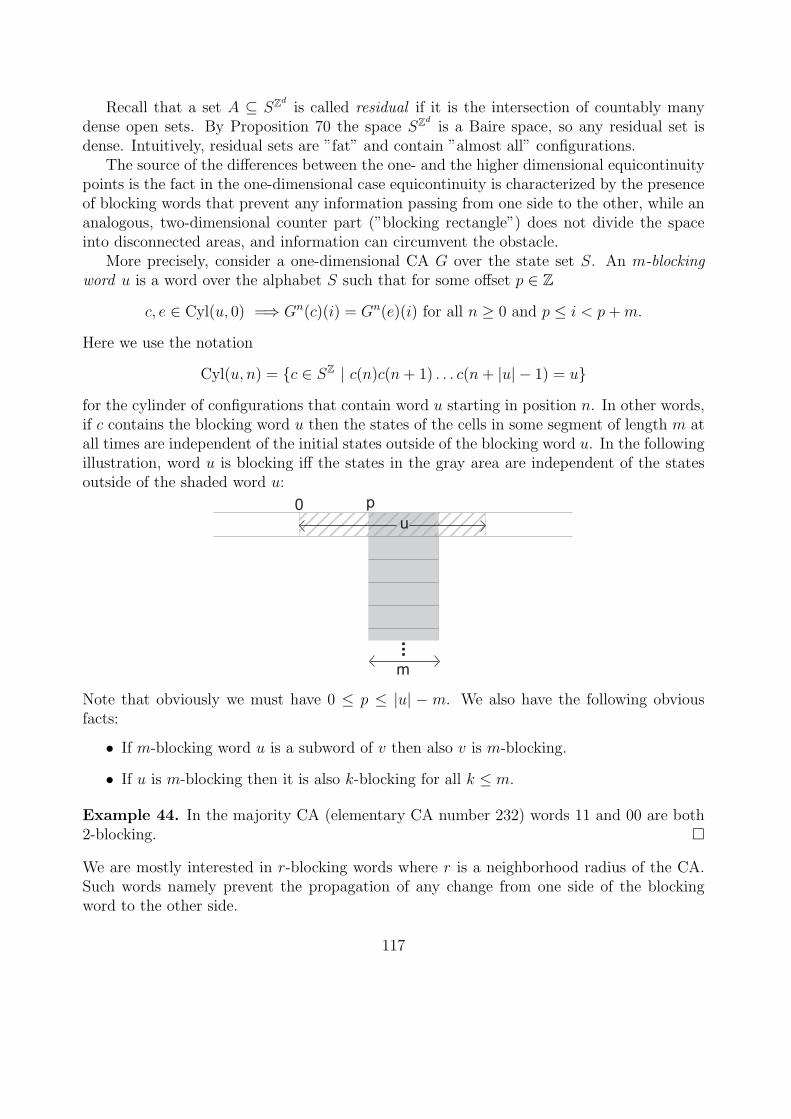
Recall that a set A ⊆ SZd

is called residual if it is the intersection of countably manydense open sets. By Proposition 70 the space SZ

dis a Baire space, so any residual set is

dense. Intuitively, residual sets are ”fat” and contain ”almost all” configurations.The source of the differences between the one- and the higher dimensional equicontinuity

points is the fact in the one-dimensional case equicontinuity is characterized by the presenceof blocking words that prevent any information passing from one side to the other, while ananalogous, two-dimensional counter part (”blocking rectangle”) does not divide the spaceinto disconnected areas, and information can circumvent the obstacle.

More precisely, consider a one-dimensional CA G over the state set S. An m-blockingword u is a word over the alphabet S such that for some offset p ∈ Z

c, e ∈ Cyl(u, 0) =⇒ Gn(c)(i) = Gn(e)(i) for all n ≥ 0 and p ≤ i < p + m.

Here we use the notation

Cyl(u, n) = c ∈ SZ | c(n)c(n + 1) . . . c(n + |u| − 1) = ufor the cylinder of configurations that contain word u starting in position n. In other words,if c contains the blocking word u then the states of the cells in some segment of length m atall times are independent of the initial states outside of the blocking word u. In the followingillustration, word u is blocking iff the states in the gray area are independent of the statesoutside of the shaded word u:

u

0 p

m

Note that obviously we must have 0 ≤ p ≤ |u| − m. We also have the following obviousfacts:

• If m-blocking word u is a subword of v then also v is m-blocking.

• If u is m-blocking then it is also k-blocking for all k ≤ m.

Example 44. In the majority CA (elementary CA number 232) words 11 and 00 are both2-blocking. ¤

We are mostly interested in r-blocking words where r is a neighborhood radius of the CA.Such words namely prevent the propagation of any change from one side of the blockingword to the other side.

117

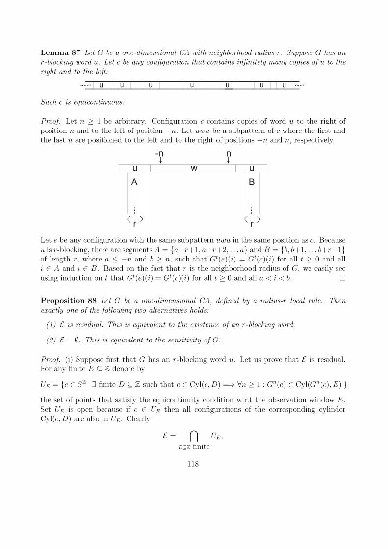
Lemma 87 Let G be a one-dimensional CA with neighborhood radius r. Suppose G has anr-blocking word u. Let c be any configuration that contains infinitely many copies of u to theright and to the left:

u u u u u u u

Such c is equicontinuous.

Proof. Let n ≥ 1 be arbitrary. Configuration c contains copies of word u to the right ofposition n and to the left of position −n. Let uwu be a subpattern of c where the first andthe last u are positioned to the left and to the right of positions −n and n, respectively.

u uw

r r

-n n

A B

Let e be any configuration with the same subpattern uwu in the same position as c. Becauseu is r-blocking, there are segments A = a−r+1, a−r+2, . . . a and B = b, b+1, . . . b+r−1of length r, where a ≤ −n and b ≥ n, such that Gt(e)(i) = Gt(c)(i) for all t ≥ 0 and alli ∈ A and i ∈ B. Based on the fact that r is the neighborhood radius of G, we easily seeusing induction on t that Gt(e)(i) = Gt(c)(i) for all t ≥ 0 and all a < i < b. ¤

Proposition 88 Let G be a one-dimensional CA, defined by a radius-r local rule. Thenexactly one of the following two alternatives holds:

(1) E is residual. This is equivalent to the existence of an r-blocking word.

(2) E = ∅. This is equivalent to the sensitivity of G.

Proof. (i) Suppose first that G has an r-blocking word u. Let us prove that E is residual.For any finite E ⊆ Z denote by

UE = c ∈ SZ | ∃ finite D ⊆ Z such that e ∈ Cyl(c,D) =⇒ ∀n ≥ 1 : Gn(e) ∈ Cyl(Gn(c), E) the set of points that satisfy the equicontinuity condition w.r.t the observation window E.Set UE is open because if c ∈ UE then all configurations of the corresponding cylinderCyl(c,D) are also in UE. Clearly

E =⋂

E⊆Z finite

UE,

118

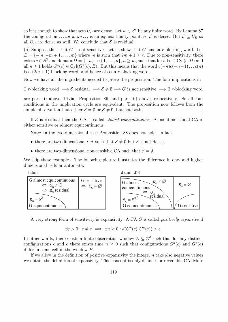
so it is enough to show that sets UE are dense. Let w ∈ S∗ be any finite word. By Lemma 87the configuration . . . uu w uu . . . is an equicontinuity point, so E is dense. But E ⊆ UE soall UE are dense as well. We conclude that E is residual.

(ii) Suppose then that G is not sensitive. Let us show that G has an r-blocking word. LetE = −m,−m + 1, . . . ,m where m is such that 2m + 1 ≥ r. Due to non-sensitivity, thereexists c ∈ SZ and domain D = −n,−n+1, . . . , n, n ≥ m, such that for all e ∈ Cyl(c,D) andall n ≥ 1 holds Gn(e) ∈ Cyl(Gn(c), E). But this means that the word c(−n)c(−n+1) . . . c(n)is a (2m + 1)-blocking word, and hence also an r-blocking word.

Now we have all the ingredients needed to prove the proposition. The four implications in

∃ r-blocking word =⇒ E residual =⇒ E 6= ∅ =⇒ G is not sensitive =⇒ ∃ r-blocking word

are part (i) above, trivial, Proposition 86, and part (ii) above, respectively. So all fourconditions in the implication cycle are equivalent. The proposition now follows from thesimple observation that either E = ∅ or E 6= ∅, but not both. ¤

If E is residual then the CA is called almost equicontinuous. A one-dimensional CA iseither sensitive or almost equicontinuous.

Note: In the two-dimensional case Proposition 88 does not hold. In fact,

• there are two-dimensional CA such that E 6= ∅ but E is not dense,

• there are two-dimensional non-sensitive CA such that E = ∅.We skip these examples. The following picture illustrates the difference in one- and higherdimensional cellular automata:

EG

¹ Æ

EG

residualÛ

G almost equicontinuous

ÛE

G= ÆÛ

G sensitive

EG

= SÙ

EG

= SÙ

d

G equicontinuous

1 dim

EG

¹ ÆG almostequicontinuous

EG

= Æ

G sensitiveG equicontinuous

d dim, d>1

EG

residualÛ

A very strong form of sensitivity is expansivity. A CA G is called positively expansive if

∃ε > 0 : c 6= e =⇒ ∃n ≥ 0 : d(Gn(c), Gn(e)) > ε.

In other words, there exists a finite observation window E ⊆ Zd such that for any distinctconfigurations c and e there exists time n ≥ 0 such that configurations Gn(c) and Gn(e)differ in some cell in the window E.

If we allow in the definition of positive expansivity the integer n take also negative valueswe obtain the definition of expansivity. This concept is only defined for reversible CA. More

119

precisely, a reversible CA is called expansive if there exists a finite E such that for any twodifferent configurations c and e there exists an integer n (which may be also negative) suchthat Gn(c) and Gn(e) differ in some cell in domain E.

Example 45. Non-zero translations are not positively expansive but in the one-dimensionalcase they are expansive. The xor CA is not positively expansive because differences onlypropagate to the left, but the three neighbor xor (elementary CA 150, local rule f(a, b, c) ≡a + b + c (mod 2)) is positively expansive. ¤

Our first observation is that expansivity and positive expansivity are stronger conditionsthan sensitivity to initial conditions.

Proposition 89 Expansive and positively expansive CA are sensitive.

Proof. For positive expansivity this is clear since the space SZd

does not have any isolatedpoints. If E is the finite observation window confirming positive expansivity of G then thesame E also confirms sensitivity: For any finite D ⊆ Zd and any c ∈ SZ

dthere exist a

configuration e ∈ Cyl(c,D) such that e 6= c. By positive expansivity, Gn(e)(~x) 6= Gn(c)(~x)for some n ≥ 0 and ~x ∈ E. This proves sensitivity.

Suppose then that reversible G is expansive, and let E be a finite observation windowconfirming its expansivity. Let D ⊆ Zd and c ∈ SZ

dbe arbitrary. It is enough to show that

for some e ∈ Cyl(c,D), some n ≥ 0 and some ~x ∈ E we have Gn(e)(~x) 6= Gn(c)(~x). Byexpansivity, such n and ~x exist for every e 6= c, except that time n may be negative. If n ≥ 0the proof is complete, so suppose now that Gn(e)(~x) 6= Gn(c)(~x) where n < 0. In reversibleCA periodic points are dense, so there exist periodic c′ and e′ such that c′, e′ ∈ Cyl(c, D),and Gn(e′)(~x) = Gn(e)(~x) 6= Gn(c)(~x) = Gn(c′)(~x). If p is a common period for c′ and e′

we have that Gn+kp(e′)(~x) = Gn(e′)(~x) 6= Gn(c′)(~x) = Gn+kp(c′)(~x), for every k ∈ Z. Forsufficiently large k the time n + kp is positive, so either c′ or e′ confirms the sensitivity. ¤

It is also easy to see that positively expansive CA must be surjective.

Proposition 90 Positively expansive CA G is surjective.

Proof. By the Garden-of-Eden -theorem, if G is not surjective then there are two configura-tions c, e such that G(c) = G(e) but the difference set

diff (c, e) = ~n ∈ Zd | c(~n) 6= e(~n)

is finite and non-empty. By translation invariance, for any observation window E we canchoose c and e in such a way that E ∩ diff (c, e) = ∅. This contradicts positive expansivity,as the difference of c and e is never seen inside the window E. ¤

The following two propositions show that only one-dimensional CA can be positivelyexpansive or expansive, and that reversible CA can never be positively expansive.

120

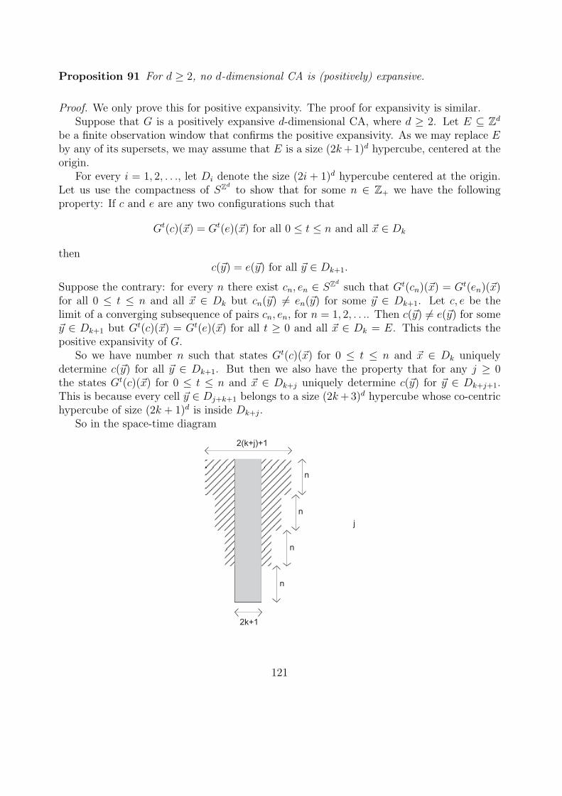
Proposition 91 For d ≥ 2, no d-dimensional CA is (positively) expansive.

Proof. We only prove this for positive expansivity. The proof for expansivity is similar.Suppose that G is a positively expansive d-dimensional CA, where d ≥ 2. Let E ⊆ Zd

be a finite observation window that confirms the positive expansivity. As we may replace Eby any of its supersets, we may assume that E is a size (2k + 1)d hypercube, centered at theorigin.

For every i = 1, 2, . . ., let Di denote the size (2i + 1)d hypercube centered at the origin.Let us use the compactness of SZ

dto show that for some n ∈ Z+ we have the following

property: If c and e are any two configurations such that

Gt(c)(~x) = Gt(e)(~x) for all 0 ≤ t ≤ n and all ~x ∈ Dk

thenc(~y) = e(~y) for all ~y ∈ Dk+1.

Suppose the contrary: for every n there exist cn, en ∈ SZd

such that Gt(cn)(~x) = Gt(en)(~x)for all 0 ≤ t ≤ n and all ~x ∈ Dk but cn(~y) 6= en(~y) for some ~y ∈ Dk+1. Let c, e be thelimit of a converging subsequence of pairs cn, en, for n = 1, 2, . . .. Then c(~y) 6= e(~y) for some~y ∈ Dk+1 but Gt(c)(~x) = Gt(e)(~x) for all t ≥ 0 and all ~x ∈ Dk = E. This contradicts thepositive expansivity of G.

So we have number n such that states Gt(c)(~x) for 0 ≤ t ≤ n and ~x ∈ Dk uniquelydetermine c(~y) for all ~y ∈ Dk+1. But then we also have the property that for any j ≥ 0the states Gt(c)(~x) for 0 ≤ t ≤ n and ~x ∈ Dk+j uniquely determine c(~y) for ~y ∈ Dk+j+1.This is because every cell ~y ∈ Dj+k+1 belongs to a size (2k + 3)d hypercube whose co-centrichypercube of size (2k + 1)d is inside Dk+j.

So in the space-time diagram

2k+1

n

n

n

n

2(k+j)+1

j

121

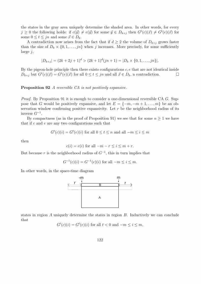
the states in the gray area uniquely determine the shaded area. In other words, for everyj ≥ 0 the following holds: if c(~y) 6= e(~y) for some ~y ∈ Dk+j then Gt(c)(~x) 6= Gt(e)(~x) forsome 0 ≤ t ≤ jn and some ~x ∈ Dk.

A contradiction now arises from the fact that if d ≥ 2 the volume of Dk+j grows fasterthan the size of Dk × 0, 1, . . . , jn when j increases. More precisely, for some sufficientlylarge j,

|Dk+j| = (2k + 2j + 1)d > (2k + 1)d(jn + 1) = |Dk × 0, 1, . . . , jn|.

By the pigeon-hole principle then there exists configurations c, e that are not identical insideDk+j but Gt(c)(~x) = Gt(e)(~x) for all 0 ≤ t ≤ jn and all ~x ∈ Dk, a contradiction. ¤

Proposition 92 A reversible CA is not positively expansive.

Proof. By Proposition 91 it is enough to consider a one-dimensional reversible CA G. Sup-pose that G would be positively expansive, and let E = −m,−m + 1, . . . , m be an ob-servation window confirming positive expansivity. Let r be the neighborhood radius of itsinverse G−1.

By compactness (as in the proof of Proposition 91) we see that for some n ≥ 1 we havethat if c and e are any two configurations such that

Gt(c)(i) = Gt(e)(i) for all 0 ≤ t ≤ n and all −m ≤ i ≤ m

thenc(i) = e(i) for all −m− r ≤ i ≤ m + r.

But because r is the neighborhood radius of G−1, this in turn implies that

G−1(c)(i) = G−1(e)(i) for all −m ≤ i ≤ m.

In other words, in the space-time diagram

r

-m m

A

Br

states in region A uniquely determine the states in region B. Inductively we can concludethat

Gt(c)(i) = Gt(e)(i) for all t < 0 and −m ≤ i ≤ m,

122

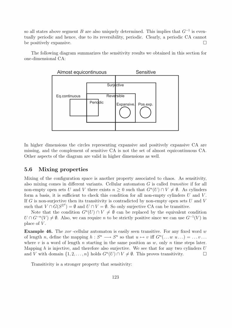
so all states above segment B are also uniquely determined. This implies that G−1 is even-tually periodic and hence, due to its reversibility, periodic. Clearly, a periodic CA cannotbe positively expansive. ¤

The following diagram summarizes the sensitivity results we obtained in this section forone-dimensional CA:

SensitiveAlmost equicontinuous

Eq.continuous

Surjective

Reversible

PeriodicPos.exp.Expansive.

In higher dimensions the circles representing expansive and positively expansive CA aremissing, and the complement of sensitive CA is not the set of almost equicontinuous CA.Other aspects of the diagram are valid in higher dimensions as well.

5.6 Mixing properties

Mixing of the configuration space is another property associated to chaos. As sensitivity,also mixing comes in different variants. Cellular automaton G is called transitive if for allnon-empty open sets U and V there exists n ≥ 0 such that Gn(U) ∩ V 6= ∅. As cylindersform a basis, it is sufficient to check this condition for all non-empty cylinders U and V .If G is non-surjective then its transitivity is contradicted by non-empty open sets U and Vsuch that V ∩G(SZ

d) = ∅ and U ∩ V = ∅. So only surjective CA can be transitive.

Note that the condition Gn(U) ∩ V 6= ∅ can be replaced by the equivalent conditionU ∩G−n(V ) 6= ∅. Also, we can require n to be strictly positive since we can use G−1(V ) inplace of V .

Example 46. The xor -cellular automaton is easily seen transitive. For any fixed word wof length n, define the mapping h : Sn −→ Sn so that u 7→ v iff Gn(. . . w u . . .) = . . . v . . .where v is a word of length n starting in the same position as w, only n time steps later.Mapping h is injective, and therefore also surjective. We see that for any two cylinders Uand V with domain 1, 2, . . . , n holds Gn(U) ∩ V 6= ∅. This proves transitivity. ¤

Transitivity is a stronger property that sensitivity:

123

Proposition 93 A transitive CA (with at least two states) is sensitive to initial conditions.

Proof. Let G be a CA that is not sensitive. Because G is not sensitive there exists someconfiguration c ∈ SZ

dand a finite domain D ⊆ Zd such that

e ∈ Cyl(c, D) =⇒ Gt(e)(~0) = Gt(c)(~0) for all t ≥ 0.

Denote C = Cyl(c,D). Let τ = τ~n be a translation by some vector ~n 6= ~0 such thatU = τ−1(C) ∩ C 6= ∅. Such a translation exists because the domain D is finite. Set U is anon-empty cylinder. Let e ∈ U be arbitrary, so e ∈ C and τ(e) ∈ C. For all t ≥ 0

Gt(e)(~n) = τ(Gt(e))(~0) = Gt(τ(e))(~0) = Gt(c)(~0) = Gt(e)(~0).

We conclude that Gt(U) ∩ V = ∅ for all t ≥ 0 where V is any cylinder with domain ~0, ~nand with different state assigned to ~0 and ~n. Hence G is not transitive. ¤

Example 47. As an example of a surjective CA that is sensitive but not transitive, considerthe product τ×I of a non-zero translation τ and the identity function I, both over the binarystate set 0, 1. This CA is sensitive because τ is sensitive, but it is not transitive becauseI is not transitive. ¤

The following proposition characterizes transitive systems in terms of orbits. Let usdenote by

TG = T = c ∈ SZd | the orbit c, G(c), G2(c), . . . is dense

the set of transitive points of G, i.e., those points whose orbit is dense.

Proposition 94 The following three conditions are equivalent for a CA G:

(i) G is transitive,

(ii) TG is a residual set,

(iii) TG 6= ∅.

Proof. ”(i) =⇒ (ii)” Suppose that G is transitive. Let U1, U2, . . . be the set of all cylinders.For each cylinder Un, let

Xn = c ∈ SZd | Gm(c) ∈ Un for some m ≥ 0

be the set of all points whose forward orbits intersect Un. Then

TG = ∩∞i=0Xn,

so it is sufficient so show that each Xn is open and dense. If c ∈ Xn then there is m suchthat Gm(c) ∈ Un. Function Gm is continuous, so G−m(Un) is an open neighborhood of c that

124

is a subset of Xn. Hence Xn is open. For denseness consider an arbitrary open set U . Bytransitivity of G there exists m such that Gm(U) ∩ Un 6= ∅, that is, U ∩Xn 6= ∅.”(ii) =⇒ (iii)” follows form the fact that SZ

dis a Baire space.

”(iii) =⇒ (i)” Suppose that c has dense forward orbit, and let U and V be arbitrary non-empty open sets. By the denseness of the orbit we have that Gn(c) ∈ U for some n.Because V ′ = V \ c,G(c), G2(c), . . . , Gn(c) is non-empty and open, there exists m suchthat Gm(c) ∈ V ′. Clearly m > n and Gm(c) ∈ V , so Gm−n(U) ∩ V 6= ∅. Hence the CA istransitive. ¤

We can make the following easy observation concerning attractors of transitive CA:

Proposition 95 The limit set SZd

is the only attractor of a transitive CA.

Proof. Suppose U is a clopen set satisfying G(U) ⊆ U . If U is not the whole space SZd

thenthere is another clopen set V such that U ∩ V = ∅. But since Gn(U) ⊆ U for all n, we haveGn(U)∩V = ∅ for all n, which means that G is not transitive. We conclude that a transitiveCA can only have one attractor, specified by U = SZ

d. ¤

The following examples shows that the converse is not true.

Example 48. Consider the CA G = H σ due to Coven and Hedlund, where H is theelementary CA number 180 and σ is the left shift. It is a one-dimensional, binary state CAwith neighborhood (0, 1, 2). In H, the state of a cell is swapped if and only if it is followedby word 10.

Let us show that H is surjective and non-sensitive (and hence non-transitive) but thelimit set Ω = SZ is the only attractor. The surjectivity of H is clear since the elementaryCA 180 is left-permutive. Non-sensitivity follows from the fact that 000 is a two-blockingword (exercise, based on the fact that the only preimage of word wn = 00(11)n10 that beginswith 00 is wn+1 = 00(11)n+110.)

Let E = a, a + 1, . . . , b be any finite contiguous domain, and let C1, C2, . . . , Cn be thecylinders with domain E. If we build a directed graph with n vertices C1, C2, . . . , Cn, andput an edge Ci −→ Cj if and only if G(Ci) ∩ Cj 6= ∅ then one can show that the graphis strongly connected. We say that the CA is chain transitive. If U 6= ∅, SZ is any clopenset then it is a union of some cylinders Ci for some domain E. Due to chain transitivityG(Ci) ∩ Cj 6= ∅ for some Ci ⊆ U and Cj ⊆ SZ \ U . Hence G(U) 6⊆ U . It follows that thelimit set SZ is the only attractor. ¤

Motivated by the example above, let us define a weaker form of transitivity. A CA iscalled chain transitive if for every c, e ∈ SZ

dand every finite D ⊆ Zd there exists a sequence

c0, c1, . . . , cn of configurations such that c0 = c, cn = e and for every i = 1, 2, . . . , n we haveG(ci−1) ∈ Cyl(ci, D). In other words, for all domains D, the following directed graph mustbe strongly connected: The vertices are the cylinders Ci with domain D, and there is anedge Ci −→ Cj iff G(Ci) ∩ Cj 6= ∅.

125

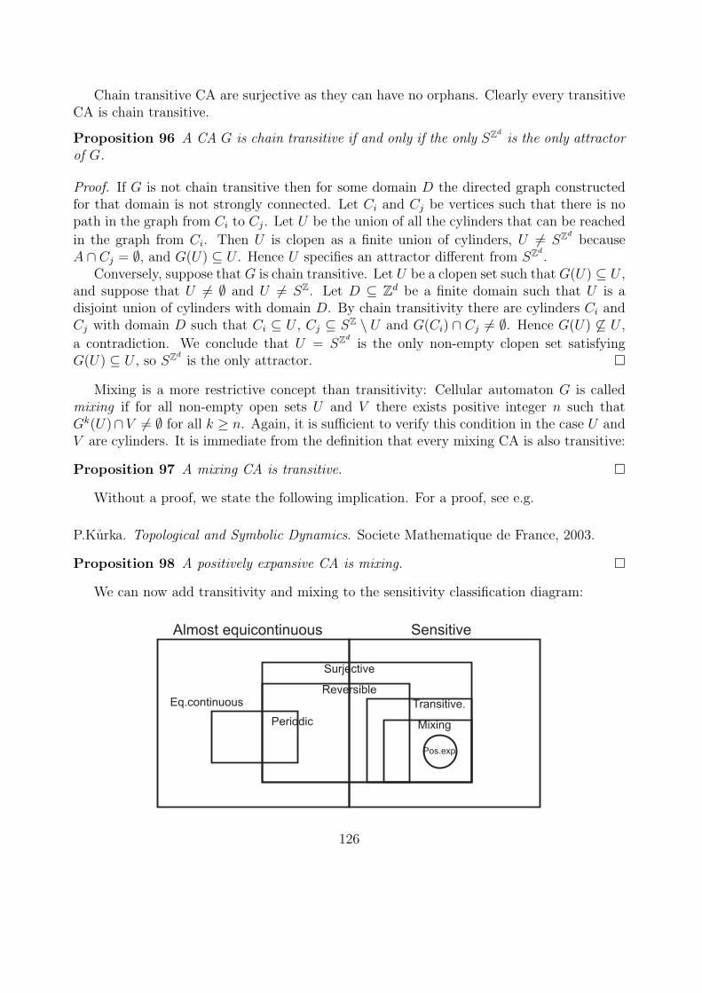
Chain transitive CA are surjective as they can have no orphans. Clearly every transitiveCA is chain transitive.

Proposition 96 A CA G is chain transitive if and only if the only SZd

is the only attractorof G.

Proof. If G is not chain transitive then for some domain D the directed graph constructedfor that domain is not strongly connected. Let Ci and Cj be vertices such that there is nopath in the graph from Ci to Cj. Let U be the union of all the cylinders that can be reached

in the graph from Ci. Then U is clopen as a finite union of cylinders, U 6= SZd

becauseA ∩ Cj = ∅, and G(U) ⊆ U . Hence U specifies an attractor different from SZ

d.

Conversely, suppose that G is chain transitive. Let U be a clopen set such that G(U) ⊆ U ,and suppose that U 6= ∅ and U 6= SZ. Let D ⊆ Zd be a finite domain such that U is adisjoint union of cylinders with domain D. By chain transitivity there are cylinders Ci andCj with domain D such that Ci ⊆ U , Cj ⊆ SZ \ U and G(Ci) ∩ Cj 6= ∅. Hence G(U) 6⊆ U ,

a contradiction. We conclude that U = SZd

is the only non-empty clopen set satisfyingG(U) ⊆ U , so SZ

dis the only attractor. ¤

Mixing is a more restrictive concept than transitivity: Cellular automaton G is calledmixing if for all non-empty open sets U and V there exists positive integer n such thatGk(U)∩V 6= ∅ for all k ≥ n. Again, it is sufficient to verify this condition in the case U andV are cylinders. It is immediate from the definition that every mixing CA is also transitive:

Proposition 97 A mixing CA is transitive. ¤

Without a proof, we state the following implication. For a proof, see e.g.

P.Kurka. Topological and Symbolic Dynamics. Societe Mathematique de France, 2003.

Proposition 98 A positively expansive CA is mixing. ¤

We can now add transitivity and mixing to the sensitivity classification diagram:

SensitiveAlmost equicontinuous

Eq.continuous

Surjective

Reversible

Periodic

Pos.exp.

Transitive.

Mixing

126

The relationship of reversible, expansive CA to transitivity and mixing is not known, soexpansive CA were excluded from the diagram.

Note that the concepts concerning sensitivity and transitivity are not just CA relatednotions, but they are concepts defined in the same way in the context of general topologicaldynamical systems. (The sensitivity related concepts require that the space has a metric,while for transitivity and mixing only the topology is needed.) Devaney defines a chaoticdynamical system to be a system that

1. is sensitive to initial conditions,

2. is transitive, and

3. temporally periodic points are dense.

We proved in proposition 93 that transitivity always implies sensitivity in cellular automata,so transitivity and dense periodic orbits characterize chaotic CA. It is also conjectured (butnot proven!) that all surjective CA have dense periodic orbits, and if true, this would implythat in cellular automata transitivity is equivalent to chaos.

Open Problem. Is it true that in every surjective CA every cylinder contains a temporallyperiodic configuration ? ¤

Among reversible CA temporally periodic configurations are dense (because spatially to-tally periodic configurations are also temporally periodic), so among reversible CA Devaney’schaos is equivalent to transitivity.

5.7 Measure invariance in surjective CA

One useful tool not yet used by us is the invariance of the uniform measure under surjectiveCA (i.e., the balance property stated in Proposition 13). Let us start by recalling some basicdefinitions of ergodic theory. Let us denote X = SZ

d. A non-empty family Σ of subsets of

X is called a σ-algebra if its is closed under complementation and countable unions, that is,if

A ∈ Σ =⇒ X \ A ∈ ΣA1, A2, . . . ∈ Σ =⇒ A1 ∪ A2 ∪ . . . ∈ Σ.

The Borel σ-algebra B is the smallest σ-algebra that contains all open sets. (It is well definedas the intersection of all σ-algebras that contain the open sets.) From now on, B denotesthe Borel σ-algebra, and its elements are called Borel sets or (Borel) measurable sets. Thefollowing results (Dynkin’s π-λ Theorem) is needed later. For a proof, see any textbook onmeasures:

Lemma 99 Let Γ be a family of subsets of X that is closed under finite intersections (so-called π-system). Let ∆ be a family of subsets of X that contains X and is closed undercomplementation and countable unions of pairwise disjoint sets (so-called λ-system). If Γ ⊆∆ then there exists a σ-algebra Σ such that Γ ⊆ Σ ⊆ ∆. ¤

127

For any continuous function G : X −→ X and any Borel measurable set A, the set G−1(A)is also Borel measurable. (The family Σ consisting of all A ⊆ X such that G−1(A) ∈ B iseasily seen to be a σ-algebra. For open U the set G−1(U) is open and hence in B, so all opensets are in Σ. It follows that B ⊆ Σ.) In particular, pre-images of measurable sets under CAfunctions are measurable.

A Borel probability measure is a function µ : B −→ R that satisfies the following condi-tions:

• µ(∅) = 0, µ(X) = 1, and µ(A) ≥ 0 for all A ∈ B, and

• (σ-additivity) If A1, A2, . . . are pairwise disjoint elements of B then

µ(A1 ∪ A2 ∪ . . .) = µ(A1) + µ(A2) + . . .

Note that σ-additivity applies to countable families of pairwise disjoint Borel sets.

Example 49. Let c ∈ X be fixed, and define

µ(A) =

1, if c ∈ A,0, if c 6∈ A.

This is easily seen to be a measure, the point measure. More generally, if C ⊆ X is finite wecan define a measure by

µ(A) =|A ∩ C||C| .

¤

Let us first show that the values of a measure on cylinders uniquely determines themeasure:

Proposition 100 If two Borel probability measures agree on cylinders then they are identi-cal.

Proof. Let Γ be the set of cylinders. Then Γ is closed under finite intersections. Suppose µ1

and µ2 be two Borel probability measures such that µ1(C) = µ2(C) for all C ∈ Γ. Let ∆ bethe family of Borel sets A such that µ1(A) = µ2(A). All cylinders are in ∆. If A ∈ ∆ then

µ1(X \ A) = 1− µ1(A) = 1− µ2(A) = µ2(X \ A),

so the complement of A is in ∆. If A1, A2, . . . are pairwise disjoint elements of ∆ then

µ1(A1 ∪ A2 ∪ . . .) = µ1(A1) + µ1(A2) + . . . = µ2(A1) + µ2(A2) + . . . = µ2(A1 ∪ A2 ∪ . . .).

We see that ∆ and Γ satisfy the conditions in Lemma 99, so there exists a σ-algebra Σ suchthat Γ ⊆ Σ ⊆ ∆. As all open sets are countable unions of cylinders we see that Σ contains

128

all open sets, and therefore all Borel sets. We conclude that µ1(A) = µ2(A) for all Borel setsA. ¤

For any Borel probability measure µ and any continuous G : X −→ X we define a newmeasure G(µ) as follows:

G(µ)(A) = µ(G−1(A)) for all A ∈ B.

The function G(µ) is defined on every Borel set A because G−1(A) is Borel. So defined G(µ)is a Borel probability measure:

Lemma 101 For any Borel probability measure µ on X and any continuous G : X −→ Xthe function G(µ) is a Borel probability measure on X.

Proof. Follows directly from the facts that G−1(∅) = ∅, G−1(X) = X, G−1(X \ A) =X \G−1(A) and

G−1(A1 ∪ A2 ∪ . . .) = G−1(A1) ∪G−1(A1) ∪ . . . .

Moreover, we need to note that G−1(Ai) and G−1(Aj) are disjoint if Ai and Aj are disjoint.¤

The measure G(µ) describes the probability distribution of configurations after one ap-plication of G, if the configurations were originally drawn according to distribution µ: TheG(µ)-probability that a configuration belongs to a measurable set A after one application ofG is the same as the µ-probability that it originally belonged to G−1(A).

We have seen that any CA G defines a function µ 7→ G(µ) on Borel probability measures.It turns out that this function can be viewed as a dynamical system because the Borelprobability measures can be given a compact metric such this application is continuous. Wedo not go into any further details of this interesting aspect.

We say that measure µ is invariant under G if G(µ) = µ. Ergodic theory is a field thatstudies dynamics under invariant measures. In the following we show that all surjective CAhave a very simple invariant measure, the uniform measure.

The simplest Borel probability measures are the Bernoulli probability measures. Givena probability distribution p : S −→ [0, 1] that satisfies

∑a∈S pa = 1, the corresponding

Bernoulli measure µp gives cylinder C = Cyl(c, D) the value

µp(C) =∏

~n∈D

p(c(~n)).

We skip the proof that this assignment on cylinders extends into a probability measure onBorel sets. (See any book on measures.)

A particular case of Bernoulli measures is the uniform probability measure that usesp(a) = 1

|S| for all a ∈ S. In this case

µp(C) =

(1

|S|)|D|

,

129

so each cylinder with the same domain is given the same probability. Under this probabilitymeasure ”each configuration has the same probability”.

Proposition 102 Let G be a surjective CA and let µ be the uniform Bernoulli measure.Then G(µ) = µ.

Proof. This is another way of stating the balance property of Proposition 13. From Propo-sition 100 we know that it is enough to show that G(µ)(C) = µ(C) for all cylindersC = Cyl(c,D′) with arbitrary finite domain D′. By Proposition 13

G−1(C) = C1 ∪ C2 ∪ . . . Cn

where Ci are disjoint cylinders with some domain D, and n = |S||D|−|D′|. We have

µ(G−1(C)) = µ(C1) + µ(C2) + . . . + µ(Cn) = n

(1

|S|)|D|

=

(1

|S|)|D′|

= µ(C).

¤

As the first application of the measure invariance we prove the following fact:

Proposition 103 Attractors of surjective CA G are exactly the clopen sets U that satisfyG(U) = U . The complement of an attractor is then also an attractor (or the empty set).

Proof. Let G be a surjective CA, and let U be any clopen set such that G(U) ⊆ U . ThenU ⊆ G−1(U). Let us prove that G−1(U) = U . Denote V = G−1(U) \U . By Proposition 102

µ(V ) = µ(G−1(U))− µ(U) = 0,

for the unform measure µ. But V is clopen, and the only open set of measure 0 is the emptyset. We conclude that G−1(U) = U . By surjectivity, G(U) = U and G(SZ

d \ U) = SZd \ U .

¤

It also follows now that the full space SZd

is the only subshift attractor (i.e. a translationinvariant attractor) of a surjective CA.

Corollary 104 The only translation invariant attractor of a surjective CA is the full spaceSZ

d.

Proof. By Proposition 103, all attractors of a surjective CA are clopen. But the onlytranslation invariant clopen sets are SZ

dand the empty set. To see this, let C be a translation

invariant clopen set, and suppose that C 6= SZd. Let U 6= ∅ be an open set such that

U ∩ C = ∅. For any translation τ , we have τ(U) ∩ C = τ(U) ∩ τ(C) = τ(U ∩ C) = ∅. But

130

then C = ∅ because for any non-empty open sets A and B there exists a translation τ suchthat τ(A) ∩B 6= ∅. ¤

One of the basic theorems of Ergodic theory is the Poincare recurrence theorem. It dealswith measure invariant transformations so it directly applies to surjective CA. We first provea variant which states that among the points inside any measurable set A, the set of pointsthat do not return back to A infinitely many times has measure zero:

Proposition 105 Let G be a surjective CA and let µ denote the uniform measure. Forevery Borel set A the set

B = c ∈ A | ∃k : ∀n > k : Gn(c) 6∈ Aof points of A that only return finitely many times to A has measure µ(B) = 0.

Proof. For every k ≥ 0 denote by

Ak = G−k(A) ∪G−k−1(A) ∪G−k−2(A) ∪ . . .

the set of points that visit A after at least k applications of G. These sets form a decreasingchain

A0 ⊇ A1 ⊇ A2 ⊇ . . .

under inclusion. Each Ak is a Borel set as a countable union of Borel sets G−i(A). Forevery k we have G−1(Ak) = Ak+1. Because the uniform measure is invariant, we haveµ(Ak) = µ(Ak+1). This means that all Ak have the same measure µ(Ak) = µ(A0).

Because A ⊆ A0, we have that A \ Ak ⊆ A0 \ Ak for every k, and consequently

µ(A \ Ak) ≤ µ(A0 \ Ak) = µ(A0)− µ(Ak) = 0.

Set B consists of those points of of A that do not belong to some Ak, that is,

B =∞⋃

k=0

(A \ Ak).

But then

µ(B) ≤∞∑

k=0

µ(A \ Ak) =∞∑

k=0

0 = 0,

which completes the proof. ¤

Remark: In particular, the set of points of A that never return to A has measure zero.(This is the set A \ A1 in the previous proof.)

A configuration is called recurrent if it returns to each of its open neighborhoods. Denoteby

RG = R = c ∈ SZd | ∀ open U : c ∈ U =⇒ ∃n ≥ 1 : Gn(c) ∈ U.

131

the set of recurrent points. If c is recurrent then it, in fact, returns infinitely many times to allits open neighborhoods U : Either c is periodic, or for every n the set U\G(c), G2(c), . . . , Gn(c)is an open neighborhood of c, which then must be visited by c. Another variant of Poincare’srecurrence theorem tells us that in surjective CA recurrent points are dense:

Proposition 106 If G is surjective then R is a countable intersection of open sets of uni-form measure 1. In particular, R is residual and µ(R) = 1.

Proof. Let U1, U2, . . . be an enumeration of all cylinders. For each k = 1, 2, . . . define

Xk = c ∈ Uk | ∀n ≥ 1 : Gn(c) 6∈ Uk.By Proposition 105 (or more precisely, the remark following the proposition) we know thatµ(Xk) = 0. Set Xk is closed because

Xk = Uk \∞⋃

n=1

G−n(Uk)

where Uk is clopen.Let us prove that

X1 ∪X2 ∪ . . . = SZd \ R.

Indeed, if c ∈ Xk then c cannot be recurrent as Uk is an open neighborhood it never returnsto. Conversely, if c is not recurrent then it has an open neighborhood U such that Gn(c) 6∈ Ufor all n = 1, 2, . . .. As cylinders form a basis, there exists k such that c ∈ Uk ⊆ U . But thenc ∈ Xk.

We conclude that

R =∞⋂

k=1

(SZd \Xk)

is a countable intersection of open sets with measure µ(SZd \Xk) = 1− µ(Xk) = 1.

To complete the proof we note that if µ(A) = 1 then A is dense (because otherwiseits complement would contain a cylinder and all cylinders have positive measure). Alsoany countable intersection of measure 1 sets has measure 1. (Because its complement is acountable union of sets of measure 0.) ¤

If a surjective CA is non-sensitive, we can now conclude that periodic points are dense:

Proposition 107 If a one-dimensional CA G is surjective and not sensitive then the peri-odic configurations are dense in SZ.

Proof. By proposition 88 there is an r-blocking word u where r is the neighborhood radiusof G. Let w ∈ S∗ be an arbitrary word. It is enough to show that there is a periodicconfiguration that contains pattern w. Let C be a cylinder determined by word uwu. ByProposition 106, cylinder C contains a recurrent configuration x so, in particular, Gn(x) ∈ Cfor some n ≥ 1.

132

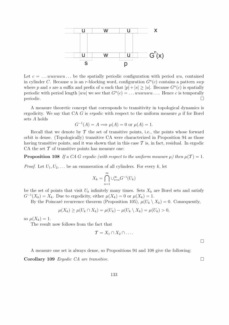
u w u

wu u

x

G (x)n

s p

Let c = . . . wuwuwu . . . be the spatially periodic configuration with period wu, containedin cylinder C. Because u is an r-blocking word, configuration Gn(c) contains a pattern swpwhere p and s are a suffix and prefix of u such that |p|+ |s| ≥ |u|. Because Gn(c) is spatiallyperiodic with period length |wu| we see that Gn(c) = . . . wuwuwu . . .. Hence c is temporallyperiodic. ¤

A measure theoretic concept that corresponds to transitivity in topological dynamics isergodicity. We say that CA G is ergodic with respect to the uniform measure µ if for Borelsets A holds

G−1(A) = A =⇒ µ(A) = 0 or µ(A) = 1.

Recall that we denote by T the set of transitive points, i.e., the points whose forwardorbit is dense. (Topologically) transitive CA were characterized in Proposition 94 as thosehaving transitive points, and it was shown that in this case T is, in fact, residual. In ergodicCA the set T of transitive points has measure one:

Proposition 108 If a CA G ergodic (with respect to the uniform measure µ) then µ(T ) = 1.

Proof. Let U1, U2, . . . be an enumeration of all cylinders. For every k, let

Xk =∞⋂

n=1

∪∞i=nG−i(Uk)

be the set of points that visit Uk infinitely many times. Sets Xk are Borel sets and satisfyG−1(Xk) = Xk. Due to ergodicity, either µ(Xk) = 0 or µ(Xk) = 1.

By the Poincare recurrence theorem (Proposition 105), µ(Uk \Xk) = 0. Consequently,

µ(Xk) ≥ µ(Uk ∩Xk) = µ(Uk)− µ(Uk \Xk) = µ(Uk) > 0,

so µ(Xk) = 1.The result now follows from the fact that

T = X1 ∩X2 ∩ . . . .

¤

A measure one set is always dense, so Propositions 94 and 108 give the following:

Corollary 109 Ergodic CA are transitive. ¤

133