cef.up working paper

2015-03

FLEXIBLE TRANSITIONAL DYNAMICS IN A NON-SCALE

FULLY ENDOGENOUS GROWTH MODEL

Pedro Mazeda Gil André Almeida

Sofia B.S.D. Castro

Flexible Transitional Dynamics in a

Non-Scale Fully Endogenous Growth

Model

Pedro Mazeda Gil,∗André Almeida,†and So�a B.S.D. Castro,‡

June 22, 2015

This paper develops a non-scale growth model of physical capital accu-mulation and two types of lab-equipment R&D, where both the intensiveand extensive margins of growth are fully endogenous. We study analyti-cally the long-run equilibrium stability and transitional dynamics propertiesof the model, and establish meaningful su�cient conditions for saddle-pathstability. We relate the di�erent combinations of initial conditions of thedynamical system with the observation of monotonic versus non-monotonictransitional dynamics. Our model is able to predict monotonic, hump-shapedand inverted hump-shaped trajectories, therefore encompassing the evidencereported by the empirical literature for distinct subsets of countries.

Keywords: endogenous growth, non-monotonic transitional dynamics, R&D, lab equip-ment, physical capital.

JEL Classi�cation: O41, O31

∗University of Porto, Faculty of Economics, and CEF.UP � Center for Economics and Finance atUniversity of Porto. Corresponding author: please email to pgil@fep.up.pt or address to Rua DrRoberto Frias, 4200-464, Porto, Portugal. Financial support from national funds by Fundação para aCiência e a Tecnologia (FCT), Portugal, as part of the Strategic Project PEst-OE/EGE/UI4105/2014.

†University of Porto, Faculty of Economics.‡University of Porto, Faculty of Economics, and CMUP. Financial support from the European Re-gional Development Fund through the programme COMPETE and from the Portuguese Governmentthrough the FCT under the project PEst-C/MAT/UI0144/2011.

1

1. Introduction

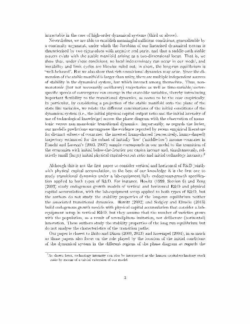
The purpose of this paper is twofold. On one hand, we study analytically the long-run equilibrium stability and transitional dynamics properties of the R&D-based growthmodel of the lab-equipment type. This is an apparently overlooked topic in the en-dogenous growth literature in favor of the models of the concurrent type, featuring aknowledge-driven R&D speci�cation. On the other hand, we carry out this study inthe context of the �exible transitional dynamics that arise in the presence of a multi-dimensional stable manifold, motivated by the empirical evidence that points out theexistence of non-monotonic transitional dynamics phenomena. Notable empirical pat-terns are: (i) the hump-shaped or inverted hump-shaped behaviour of the transitionaleconomic growth rates (see, e.g., Papageorgiou and Perez-Sebastian, 2006; Fiaschi andLavezzi, 2003a, 2007; see also Figure 1) and saving rates (Maddison, 1992; Loyaza,Schmidt-Hebbel, and Serven, 2000); (ii) the non-linear relationship between the stock ofphysical capital and the number of �rms over transition (Gil, 2010); and (iii) the time-variable and sector-speci�c speed of convergence (Bernard and Jones, 1996). Bearing theabove in mind, this paper develops a non-scale fully endogenous growth model of physicalcapital accumulation and two types of R&D � vertical (increase of product quality) andhorizontal (creation of new products) �, both under a lab-equipment speci�cation.

[Figure 1 goes about here]

The concern with the stability properties of the long-run equilibrium in R&D growthmodels and the characteristics of their transitional dynamics has occupied a signi�cantstrand of the endogenous growth literature. Several papers devoted e�orts to study inthat regard the seminal models by Romer (1990), Aghion and Howitt (1992) and Jones(1995), and a variety of extensions of those models (e.g., Arnold, 1998, 2000, 2006; Eicherand Turnovsky, 2001; Kosempel, 2004; Gómez, 2005; Arnold and Kornprobst, 2008;Sequeira, 2011; Growiec and Schumacher, 2013; Sequeira, Lopes, and Gomes, 2014).All these models are of the knowledge-driven type. In contrast, our paper focuses onthe equilibrium and transitional dynamics properties of an R&D growth model of thelab-equipment type, as laid out originally by Rivera-Batiz and Romer (1991) and Barroand Sala-i-Martin (2004) (with �rst edition in 1995). Indeed, from the perspective ofthe technology of R&D, two polar cases can be considered (Rivera-Batiz and Romer,1991): the knowledge-driven case, which assumes that human capital and knowledgeare the only inputs to R&D activities; and the lab-equipment case, which assumes thatthe technology for R&D is the same as the technology for �nal-good production, andthus human capital, raw labour, and capital goods are all productive in R&D activities.In this latter setting, physical capital accumulation and R&D complement each other,meaning that capital accumulation relates to R&D more closely than in the knowledge-driven setting. This allows one to address the empirical evidence that shows an importantinterconnection between physical and technological inputs along growth processes (e.g.,Bernard and Jones, 1996; Papageorgiou and Perez-Sebastian, 2006).The consideration of the two types of R&D follows from both a substantive (economic)

and formal (technical) argument. As for the former, such a setup enables us to address

2

Figure 1: Annual per capita GDP growth rate versus the corresponding annual per capita GDP

level, for 122 countries from 1950 to 1998, where the black solid line is a nonparamet-

ric regression line. This is a reproduction of the �gure in Fiaschi and Lavezzi (2003b,

p. 6). These authors use this cross-section of countries over time to estimate transi-

tion probabilities in a state space de�ned in terms of both income levels and growth

rates. By keeping track of the growth path of each individual country, they show that

di�erent subsets of countries with initial below-world average income � 'low' versus

'middle-low' income countries � may follow, respectively, inverted hump-shaped and

hump-shaped transitions.

3

the general view that industrial growth proceeds both along an intensive (vertical inno-vation) and an extensive (horizontal innovation) margin in the long run, as well as theevidence relating the initial intensity of use of technological knowledge (i.e., the initialproportion of the intensive vis-à-vis the extensive component of a given technological-knowledge stock) and the transitional growth rates (e.g., Jones and Romer, 2010). Inparticular, the integration of the two types of R&D in a lab-equipment setup allows us tobuild a non-scale fully endogenous growth model such that a positive growth rate arisesalong both the intensive and the extensive margin without relying on a positive (exoge-nous) population growth rate, i.e., we endogenise both margins of growth (and therebyproduction, the number of �rms, and �rm size). This stands in contrast with the usualapproaches in the knowledge-driven literature, which imply a strictly positive relationshipbetween economic growth (or its extensive margin) and the population growth rate (e.g.,Jones, 1995; Dinopoulos and Thompson, 1998; Peretto, 1998; Eicher and Turnovsky,2001),1 a result that has not received empirical support (e.g., Dinopoulos and Thomp-son, 2000; Strulik, Prettner, and Prskawetz, 2013). On the other hand, under this setup,aggregate dynamics is characterised by a third-order dynamical system in appropriatelyscaled variables, with one jump-like and two state-like variables, where the latter re-sult from the interaction between physical capital and the technological-knowledge stockobtained from the two types of R&D activities. We consider an asymmetry betweenhorizontal and vertical R&D costs (e.g., Howitt, 1999), re�ecting the inherently distinctnature of horizontal and vertical innovation, or between technology embodied in newproducts (more physical) and in improved processes/products (more immaterial). It isthis asymmetry that makes the dynamical system of third order, while preserving thefully endogenous-growth result.As stated earlier, we are interested in the long-run equilibrium stability and transi-

tional dynamics properties of this model. However, an important modelling distinctionbetween the knowledge-driven and the lab-equipment settings is that, in the former,the dynamic general equilibrium is established upon the satisfaction of (at least) twoaggregate resource constraints, pertaining to the product market and to the labour (orhuman capital) market, respectively; in the latter, only the aggregate resource constraintpertaining to the product market is relevant for the derivation of the dynamic generalequilibrium. The consequence is that, in the lab-equipment setting, the dynamical-systemequations are tied up together by this single aggregate resource constraint, implying thatthe respective Jacobian matrix is dense, with no or very few null elements, and thus thedynamical system cannot be decoupled; this makes a complete analytical study usually

1Jones' (1995) solution to the scale-e�ect result found in the �rst-generation endogenous growth mod-els (e.g., Romer, 1990; Aghion and Howitt, 1992) implied that positive economic growth relied ona positive population growth rate (the semi-endogenous growth result). As a reaction, a new gen-eration of endogenous-growth models introduced simultaneous vertical and horizontal R&D as amodelling strategy to remove scale e�ects while preserving the �rst-generation result that long-runeconomic growth has policy-sensitive economic determinants (the fully-endogenous growth result)(e.g., Dinopoulos and Thompson, 1998; Peretto, 1998; Howitt, 1999). However, in these models, theextensive margin of growth still relies on a positive population growth rate. In contrast, following,e.g., Barro and Sala-i-Martin (2004), our approach allows us to remove scale e�ects and still get thefully endogenous-growth result along both the intensive and the extensive margin.

4

intractable in the case of high-order dynamical systems (third or above).Nevertheless, we are able to establish meaningful su�cient conditions, generalisable by

a continuity argument, under which the Jacobian of our linearised dynamical system ischaracterised by two eigenvalues with negative real parts, and thus a saddle-path stablesystem exists with the stable manifold arising as a two-dimensional locus. That is, weshow that, under these conditions, no local indeterminacy can occur in our model, andinstability and limit cycles are likewise ruled out; in short, the long-run equilibrium is�well-behaved�. But we also show that rich transitional dynamics may arise. Since the di-mension of the stable manifold is larger than unity, there are multiple independent sourcesof stability in the dynamical system, but which interact among themselves. Thus, non-monotonic (but not necessarily oscillatory) trajectories as well as time-variable/sector-speci�c speeds of convergence can emerge in the state-like variables, thereby introducingimportant �exibility to the transitional dynamics, as seems to be the case empirically.In particular, by considering a projection of the stable manifold onto the plane of thestate-like variables, we relate the di�erent combinations of the initial conditions of thedynamical system (i.e., the initial physical capital-output ratio and the initial intensity ofuse of technological knowledge) across the phase diagram with the observation of mono-tonic versus non-monotonic transitional dynamics. Importantly, as regards the latter,our model's predictions encompasse the evidence reported by recent empirical literaturefor distinct subsets of countries: the inverted hump-shaped (respectively, hump-shaped)trajectory estimated for the subset of initially 'low' ('middle-low') income countries inFiaschi and Lavezzi's (2003, 2007) sample corresponds in our model to the transition ofthe economies with initial below-the-frontier per capita income and, simultaneously, rel-atively small (large) initial physical capital-output ratio and initial technology intensity.2

Although this is not the �rst paper to consider vertical and horizontal of R&D jointlywith physical capital accumulation, to the best of our knowledge it is the �rst one tostudy transitional dynamics under a lab-equipment/fully endogenous-growth speci�ca-tion applied to both types of R&D. For instance, Howitt (1999, Section 6) and Zeng(2003) study endogenous growth models of vertical and horizontal R&D and physicalcapital accumulation, with the lab-equipment setup applied to both types of R&D, butthe authors do not study the stability properties of the long-run equilibrium neitherthe associated transitional dynamics. Howitt (2002) and Sedgley and Elmslie (2013)build endogenous growth models with physical capital accumulation that consider a lab-equipment setup in vertical R&D, but they assume that the number of varieties growswith the population, as a result of serendipitous imitation, not deliberate (horizontal)innovation. These authors study the stability properties of the long-run equilibrium butdo not analyse the characteristics of the transition paths.Our paper is closest to Brito and Dixon (2009, 2013) and Kosempel (2004), in as much

as those papers also focus on the role played by the location of the initial conditionsof the dynamical system in the di�erent regions of the phase diagram as regards the

2As shown later, technology intensity can also be interpreted as the human capital-technology stockratio by means of a trivial extension of our model.

5

production of monotonic versus non-monotonic transition paths. Brito and Dixon (2009,2013) focus on the behaviour of physical capital, number of �rms and �rm size in aRamsey model of a stationary economy. Kosempel (2004) uses a growth model to studythe dynamic behaviour of the ratios of human capital and of physical capital to thetechnological-knowledge stock; however, the transition path of the economic growth rateis not explicitly analysed by the authors, while growth is exogenously given in the long runequilibrium. A key contribution is also Eicher and Turnovsky (2001), who use an R&D-based growth model of the knowledge-driven type to focus on the dynamic behaviour ofthe growth rates of per capita output, physical capital and number of �rms. However, theauthors carry out their study of the transition paths by simulating a number of exogenousshocks to speci�c structural parameters (which then set the economy o� the steady stateacross the phase diagram), instead of explicitly considering the set of alternative initialconditions in the phase diagram. In contrast, we look at the behaviour of all thosevariables both in levels and growth rates under a fully endogenous-growth framework byconsidering systematically the initial conditions located in the di�erent regions of thephase diagram.A number of other papers in the endogenous-growth literature, alreadycited above (e.g., Gómez, 2005, Arnold, 2006, Arnold and Kornprobst, 2008, Sequeira,2011, Growiec and Schumacher, 2013, Sequeira, Lopes, and Gomes, 2014), only focuson the existence of non-monotonic transitions that emerge as oscillatory trajectories, byanalysing the e�ect of shifts in the values of key structural parameters on the imaginarypart of the stable eigenvalues.The remainder of the paper is as follows. In Section 2, we present the model, derive

the dynamic general equilibrium and study the interior long-run equilibrium in terms ofits existence, uniqueness, and local dynamics properties. In Section 4, we study the richtransitional dynamics that arise in the presence of a multi-dimensional stable manifold,by considering alternative initial conditions of the dynamical system. Section 5 discussesthe results and concludes.

2. The model

We study a dynamic general equilibrium model where a single competitively-produced�nal good can be used in consumption, accumulation of physical capital, and vertical andhorizontal R&D. The economy is populated by in�nitely-lived households who inelasti-cally supply labour to �nal-good �rms. In turn, families make consumption decisionsand invest in �rms' equity. The �nal good is produced using labour and a continuum ofintermediate goods indexed by ω ∈ [0, N ]. Potential entrants into the intermediate-goodsector can devote resources either to horizontal or to vertical R&D. The former increasesthe number of intermediate-good varieties N , each produced by a speci�c industry, whilethe latter increases the quality of the intermediate good of an existing variety/industry,indexed by j(ω). The quality level j(ω) then impacts the �nal-good production by afactor λj(ω), where λ > 1 is a parameter measuring the size of each quality upgrade.

6

2.1. Production and price decisions

The �nal-good �rm has the following production technology,

Y (t) = L1−α ·ˆ N(t)

0

[λj(ω,t) ·X(ω, t)

]αdω, 0 < α < 1, λ > 1, (1)

where L is the labour input, λj(ω,t) ·X(ω, t) is the input of intermediate good ω measuredin e�ciency units,3 and N(t) is the measure of varieties of these goods, all taken at timet. Final producers are price-takers in all the markets they participate. They take wages,w(t), and input prices p(ω, t) as given and sell their output at a price equal to unity.From the pro�t maximisation conditions, we determine the demand of intermediate goodω as

X(ω, t) = L ·(λj(ω,t)α · αp(ω, t)

) 11−α

, ω ∈ [0, N(t)]. (2)

The intermediate good is non-durable and is produced using capital, according tothe production function X(ω, t) = K(ω, t), where K(ω, t) is the input of capital. In-termediate good ω is produced with a cost function r(t)K(ω, t) = r(t)X(ω, t), wherethe cost of capital is the equilibrium market real interest rate, r(t).4 The intermediate-good sector consists of a continuum N(t) of industries. There is monopolistic com-petition if we consider the whole sector: the monopolist in industry ω �xes the pricep(ω, t) but faces the isoelastic demand curve (2). Pro�t in industry ω is thus π(ω, t) =(p(ω, t)−r(t)) ·X(ω, t), and the pro�t maximising price is a markup over marginal cost,5

p(ω, t) ≡ p(t) = r(t)/α > 1, which is constant across industries but possibly variableover time. The quality of the intermediate good ω can be characterised by the qualityindex q(ω, t) ≡ λj(ω,t) α

1−α . Then, from (2) and the mark-up, the quantity produced of ω

is X(ω, t) = L ·(α2/r(t)

) 11−α · q(ω, t).

On the other hand, capital market equilibrium requires K(t) =´ N(t)

0 K(ω, t)dω =´ N(t)

0 X(ω, t)dω = X(t) ·Q(t), where X(t) ≡ L ·(α2/r(t)

) 11−α and

Q(t) =

ˆ N(t)

0q(ω, t)dω, (3)

which is the aggregate quality index. The latter measures the technological-knowledgestock of the economy, since, by assumption, there are no intersectoral spillovers. Giventhe capital market equilibrium condition, the quantity produced of ω can be expressed

3In equilibrium, only the top quality of each ω is produced and used; thus, X(j, ω, t) = X(ω, t).Henceforth, we only use all arguments (j, ω, t) if they are useful for expositional convenience.

4For sake of simplicity, we assume the rate of depreciation is zero.5We assume that 1

α≤ λ; i.e., if 1

αis the price of the top quality, the price of the next lowest grade,

1αλ

, is less than the unit marginal cost. In this case, lower grades are unable to provide any e�ectivecompetition, and the top-quality producer can charge the unconstrained monopoly price.

7

alternatively asX(ω, t) = X(t)·q(ω, t) = K(t)/Q(t)·q(ω, t). By using the two expressionsfor X(ω, t), we �nd

r(t) = α2 · k(t)α−1, (4)

where k ≡ K/(LQ). This equation expresses the condition that the cost of capital mustequal its marginal revenue product. By using X(ω, t) and r(t), we get the optimal pro�taccrued by the monopolist in ω

π(ω, t) = π0 · L · k(t)α · q(ω, t), (5)

where π0 ≡ α(1 − α) is a positive constant. Also by means of X(ω, t), we get totaloptimal pro�ts, total intermediate-good production, and total �nal-good production,

Π(t) =

ˆ N(t)

0π(ω, t)dω = π0 · L · k(t)α ·Q(t). (6)

X(t) =

ˆ N(t)

0X(ω, t)dω = k(t) · L ·Q(t) = K(t), (7)

Y (t) = L ·Q(t) · k(t)α. (8)

2.2. R&D

We consider two R&D sectors, one targeting horizontal innovation and the other verticalinnovation. Each new design (a new variety or a higher quality good) is granted a patentand thus a successful innovator retains exclusive rights over the use of his/her good. Bothvertical and horizontal R&D are performed by (potential) entrants, and successful R&Dleads to the set-up of a new �rm in either an existing or in a new industry (e.g., Howitt,1999; Strulik, 2007; Gil, Brito, and Afonso, 2013). There is perfect competition amongentrants and free entry in R&D business.

2.2.1. Vertical R&D

By improving on the current top quality level j(ω, t), a successful vertical R&D �rm earnsmonopoly pro�ts from selling the leading-edge input of j(ω, t) + 1 quality to �nal-good�rms. A successful innovation will instantaneously increase the quality index in ω fromq(ω, t) = q(j) to q+(ω, t) = q(j + 1) = λα/(1−α)q(ω, t). In equilibrium, the lower qualitygood is priced out of business and the entrant replaces the incumbent monopolist, i.e.,there is a creative-destruction e�ect.Let Ii (j) denote the Poisson arrival rate of vertical innovations (vertical-innovation

rate) by potential entrant i in industry ω when the highest quality is j. Rate Ii (j) isindependently distributed across �rms, across industries and over time, and depends onthe �ow of resources Rvi (j) committed by potential entrant at time t, measured in unitsof the �nal good (e.g., Barro and Sala-i-Martin, 2004, ch. 7). Rate Ii (j) features constantreturns in R&D expenditures, Ii (j) = Rvi (j) /Φ (j), where the cost Φ (j) is homogeneous

8

across i in industry ω. Aggregating across i in ω, we get Rv (j) =∑

iRvi (j) andI (j) =

∑i Ii (j), and thus

I(j) =1

Φ(j)Rv(j), (9)

where Φ(j) = ζ · L · q(j + 1), and ζ > 0 is a constant (�ow) �xed cost. This equationincorporates an R&D complexity e�ect, implying that the larger the level of quality, q,the costlier it is to introduce a further jump in quality.6 It also incorporates a marketcomplexity e�ect, implying that an increase in market scale dilutes the e�ect of R&Doutlays on innovation probability; this captures the idea that the di�culty of introducingnew qualities and replacing old ones is proportional to the market size measured byemployed labour in e�ciency units and removes the undesirable scale e�ects on growth(e.g., Barro and Sala-i-Martin, 2004, ch. 7; Etro, 2008).As the terminal date of each monopoly arrives as a Poisson process with frequency

I (j) per (in�nitesimal) increment of time, the present value of a monopolist's pro�ts is arandom variable. Let V (j) denote the expected value of an incumbent �rm with currentquality level j(ω, t),7

V (j) = π0 · L · q(j)ˆ ∞

tk(t)α · e−

´ st (r(v)+I(j))dvds (10)

where r is the equilibrium market real interest rate and π0 · L · q(j) = π · k−α, given by(5), is constant in-between innovations. Because physical capital and R&D investmentboth represent foregone consumption (see Subsection 2.5, below), the real rate of returnto R&D is equal to that for capital, r. Free-entry prevails in vertical R&D such that thecondition I(j) · V (j + 1) = Rv (j) holds, and thus V (j + 1) = Φ (j) = ζ · L · q(j + 1).Next, we determine V (j + 1) analogously to (10) and time-di�erentiate the resultingexpression. If we also consider (5), we get the no-arbitrage condition facing a verticalinnovator

r(t) + I(t) =π0 · k(t)α

ζ(11)

It has the implication that the rates of vertical entry are symmetric across industries,I(ω, t) = I(t).8

Solving equation (9) for Rv(ω, t) = Rv(j) and aggregating across industries ω, we

determine total resources devoted to vertical R&D, Rv (t) =´ N(t)

0 Rv (ω, t) dω =´ N(t)

0 ζ ·L · q+(ω, t) · I (ω, t) dω. As the innovation rate is industry independent, then

6The way Φ depends on j implies that the increasing di�culty of creating new qualities exactly o�setsthe increased rewards from marketing higher qualities � see (9) and (5). This allows for a constantvertical-innovation rate over t and across ω along the BGP, i.e., a symmetric equilibrium.

7We assume that entrants are risk-neutral and, thus, only care about the expected value.8Observe that, from (5) and (9), we have π(ω,t)

π(ω,t)− α k(t)

k(t)= I(ω, t) ·

[j(ω, t) ·

(α

1−α

)· lnλ

]and

Rv(ω,t)Rv(ω,t)

− I(ω,t)I(ω,t)

= I(ω, t) ·[j(ω, t) ·

(α

1−α

)· lnλ

]. Then, if we time-di�erentiate the free-entry condi-

tion considering (10) and the equations above, we get r(t) = π(j+1)·I(j)Rv(j)

− I(j + 1), which can then

be re-written as (11).

9

Rv (t) = ζ · L · λ α1−α · I(t) ·Q(t). (12)

2.2.2. Horizontal R&D

Variety expansion arises from R&D aimed at creating a new intermediate good. Underperfect competition among R&D �rms and constant returns to scale at the �rm level,

instantaneous entry is obtained as.N e(t) = Rne (t) /η(t), where

.N e(t) is the contribution

to the instantaneous �ow of the new good by potential entrant e at a cost of η(t) andRne (t) is the �ow of resources devoted to horizontal R&D by e at time t, measured inunits of the �nal good (e.g., Barro and Sala-i-Martin, 2004, ch. 6). The cost η is assumed

to be symmetric. Then, Rn =∑

eRne and.N(t) =

∑e

.N e(t), implying

N(t) =1

η(t)Rn(t). (13)

Following Gil, Brito, and Afonso (2013), we assume that the cost of horizontal entry isincreasing in both the number of existing varieties, N , and the number of new entrants,N , η(t) = φ · N(t)σ · N(t)γ , where φ > 0 is a constant (�ow) �xed cost, and σ, γ >0. This equation introduces two types of decreasing returns associated to horizontalR&D. Dynamic decreasing returns to scale are modeled by the dependence of η on Nand capture an R&D complexity e�ect: the larger the number of existing varieties, thecostlier it is to introduce new varieties. The dependence of η on N means that the entrytechnology displays static decreasing returns to scale at the aggregate level, due to, e.g.,congestion e�ects re�ecting the physical nature of this type of R&D (in contrast with themore immaterial nature of vertical R&D). We assume these to be entirely external to the�rm. An implication is that new varieties are brought to the market gradually, insteadof through a lumpy adjustment. This is in line with the stylised facts on entry (e.g.,Geroski, 1995), according to which entry occurs mostly at small scale since adjustmentcosts penalise large-scale entry. The existing growth literature of horizontal R&D dealswith the two features separately: some models only display dynamic decreasing returns(e.g., Evans, Honkapohja, and Romer, 1998; Barro and Sala-i-Martin, 2004, ch. 6), whileothers only assume static decreasing returns (e.g., Arnold, 1998; Howitt, 1999; Jones andWilliams, 2000).The innovator enters with a new intermediate good whose quality level is drawn ran-

domly from the distribution of existing varieties (e.g., Howitt, 1999). Thus, the expected

quality level of the horizontal innovator is q(t) =´ N(t)

0 q(ω, t)dω/N(t) = Q(t)/N(t). Asmonopoly power will be also terminated by the arrival of a successful vertical innovatorin the future, the bene�ts from entry are given by

V (q) = π0 · L · q(t)ˆ ∞

tk(t)α · e−

´ st [r(ν)+I(q)]dνds, (14)

10

where π0Lq = πk−α. The free-entry condition is now N · V (q) = Rn, which simpli�esto V (q) = η(t). Using (14) and time-di�erentiating the resulting expression, yields theno-arbitrage condition facing a horizontal innovator

r (t) + I(t) =π(t)

η (t). (15)

Total resources devoted to horizontal R&D are given by Rn(t) = η(t)N(t), from (13).

2.2.3. Inter-R&D no-arbitrage condition

Before deciding which type of R&D to perform, the potential entrant should evaluate thebest type of entry. At the margin, she/he should be indi�erent between the two types.If we equate the e�ective rate of return r+ I for both types of entry by considering (11)and (15), we get the no-arbitrage condition

q(t) =Q (t)

N (t)=η (t)

ζ · L, (16)

which equates the cost of horizontal R&D, η, to the average cost of vertical R&D, qζL.Equation (16) can be equivalently recast as

N(t) = x(Q(t), N(t)) ·N(t), (17)

where

x(Q,N) =

(ζ · Lφ

) 1γ

·Q1γ ·N−

(σ+γ+1γ

), (18)

which expresses a channel between vertical innovation and �rm dynamics. It shows thatthe horizontal-entry rate, N/N , depends negatively on N and positively on Q: the �rstrelationship results from the complexity e�ect incorporated in equation (13), and thesecond is an implication of the complementarity between the horizontal-entry rate andthe technological-knowledge stock, which in turn comprises both the horizontal and thevertical-innovation components, Q = N · q. By time-di�erentiating q = Q/N using (3),we see that the rate of growth of average quality is equal to the expected arrival rate ofa vertical innovation multiplied by the quality shift it introduces: q(t)/q(t) = Ξ · I(t),

where both the quality shift, Ξ ≡ (q+− q)/q =(λ

α1−α − 1

)(which captures the creative-

destruction e�ect), and the vertical-innovation rate, I, are industry-independent. Then,using (17), we get

Q(t) = (I(t) · Ξ + x(Q(t), N(t))) ·Q(t), (19)

The vertical-innovation rate is endogenous and will be determined as an economy-widefunction below. Equation (19) introduces a second dynamic interaction between the twotypes of entry, in this case between the number of varieties, N , and the rate of growthof the quality index of the economy.

11

2.3. Households

The economy is populated by a constant number of in�nitely-lived households who con-sume and earn income from investments in �nancial assets (equity) and from labour.Households inelastically supply labour to �nal-good �rms; thus, total labour supply, L,is exogenous and constant. Consumers have perfect foresight regarding the technolog-ical change over time and choose the path of aggregate consumption {C(t), t ≥ 0} tomaximise discounted lifetime utility

U =

ˆ ∞

0

(C(t)1−θ − 1

1− θ

)· e−ρtdt, (20)

where ρ > 0 is the subjective discount rate and θ > 0 is the inverse of the intertemporalelasticity of substitution in consumption, subject to the �ow budget constraint

a(t) = r(t) · a(t) + w(t) · L− C(t), (21)

where a denotes households' real �nancial assets holdings and its initial level, a(0), isgiven. The optimal path of consumption (Euler equation) and the transversality condi-tion are

C(t) =1

θ· (r(t)− ρ)C(t) (22)

limt→+∞

e−ρt · C(t)−θ · a(t) = 0 (23)

2.4. Macroeconomic aggregation

The aggregate �nancial wealth held by all households is a(t) = K(t) +´ N(t)

0 V (ω, t)dω,which, from the arbitrage condition between vertical and horizontal entry, yields a(t) =K(t) + η(t) ·N(t). Taking time derivatives and comparing with (21), we get an expres-sion for the aggregate �ow budget constraint which is equivalent to the product marketequilibrium condition (see Appendix A)

Y (t) = C(t) + K(t) +Rv(t) +Rn(t) (24)

If we substitute the expressions for the aggregate output (8) and for total R&D expen-ditures (12) and (13), and then solve for K using (16) and (17), we get the endogenousrate of physical-capital accumulation

K(t) = L ·Q(t) ·(k (t)α − C(t)

L ·Q(t)− ζ · x(Q(t), N(t))− I(t) · ζ · λ α

1−α

)(25)

In parallel, recall (4) and (11), to get r(t) ≡ r(Q,K) and hence the endogenous vertical-innovation rate,

12

I(Q,K) =π0 · k(t)α

ζ− r(Q,K), (26)

as a function which is decreasing in the aggregate quality level and increasing in thephysical-capital stock. As function I(Q,K) may be negative, the relevant innovationrate at the macroeconomic level is I+(Q,K) = max {I(Q,K), 0}. We emphasise thecomplementarity between vertical innovation and physical-capital accumulation, heremade clear by the fact that, if K is too low, vertical R&D shuts down (i.e., I+ (·) = 0).

2.5. Dynamic general equilibrium

The dynamic general equilibrium is de�ned by the allocation {X(ω, t), ω ∈ [0, N(t)], t ≥ 0},by the prices {p(ω, t), ω ∈ [0, N(t)], t ≥ 0} and by the aggregate paths {C(t), N(t), Q(t),K(t), I(t), r(t), t ≥ 0}, such that: (i) consumers, �nal-good �rms and intermediate-good�rms solve their problems; (ii) vertical, horizontal and consistency free-entry conditionsare met; and (iii) markets clear. We focus on the region of the state space whereI+ (·) = I (·) > 0, such that the equilibrium paths can be obtained from the system

C =1

θ· (r(Q,K)− ρ) · C (27)

Q = (I(Q,K) · Ξ + x(Q,N)) ·Q (28)

K = LQ ·(kα − C

LQ− ζ · x(Q,N)− I(Q,K) · ζ · λ α

1−α

)(29)

N = x(Q,N) ·N (30)

given K(0), Q(0) and N(0), and the transversality condition (23), which may be re-written as

limt→+∞

e−ρt · C(t)−θ · (K(t) + ζ · L ·Q(t)) = 0 (31)

3. Equilibrium dynamics

3.1. Balanced-growth path

Let gy ≡ y/y denote the growth rate of variable y(t). As the functions in system (27)-(29) are homogeneous, a balanced-growth path (BGP) may exist if the further necessaryconditions are veri�ed: (i) the asymptotic growth rates of consumption, of physical capitaland of technological knowledge are constant and equal, gC = gK = gK = gQ = g;(ii) the vertical-innovation rate and the real interest rate are asymptotically trendless,gI = gr = 0; and (iii) the asymptotic growth rates of the quality index and the numberof varieties are monotonically related, gQ = (σ + γ + 1) · gN . Observe, from (18), thatx = gN is always positive if N > 0.

13

Under these conditions, recall (18) and k(t) ≡ K(t)/(L ·Q(t)), and let z(t) ≡ C(t)/(L ·Q(t)), with the property that, along the BGP, x = z = k = 0. Then, it is easily shownthat the system (27)-(29) is equivalent to

x(t) =

[I(k(t)) · Ξ · 1

γ−(σ

γ+ 1

)· x(t)

]· x(t) (32)

z(t) =

[1

θ· (r(k(t))− ρ)− Ξ · I(k(t))− x(t)

]· z(t) (33)

k(t) =

[1

k(t)·(k(t)α − z(t)− ζ · x(t)− ζ · λ α

1−α · I(k(t)))− Ξ · I(k(t))− x(t)

]· k(t) (34)

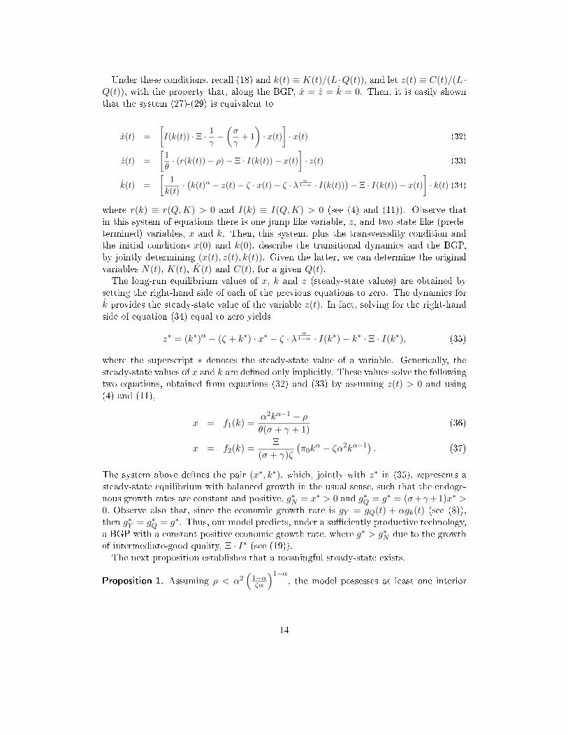
where r(k) ≡ r(Q,K) > 0 and I(k) ≡ I(Q,K) > 0 (see (4) and (11)). Observe thatin this system of equations there is one jump-like variable, z, and two state-like (prede-termined) variables, x and k. Then, this system, plus the transversality condition andthe initial conditions x(0) and k(0), describe the transitional dynamics and the BGP,by jointly determining (x(t), z(t), k(t)). Given the latter, we can determine the originalvariables N(t), K(t), K(t) and C(t), for a given Q(t).The long-run equilibrium values of x, k and z (steady-state values) are obtained by

setting the right-hand side of each of the previous equations to zero. The dynamics fork provides the steady-state value of the variable z(t). In fact, solving for the right-handside of equation (34) equal to zero yields

z∗ = (k∗)α − (ζ + k∗) · x∗ − ζ · λ α1−α · I(k∗)− k∗ · Ξ · I(k∗), (35)

where the superscript ∗ denotes the steady-state value of a variable. Generically, thesteady-state values of x and k are de�ned only implicitly. These values solve the followingtwo equations, obtained from equations (32) and (33) by assuming z(t) > 0 and using(4) and (11),

x = f1(k) =α2kα−1 − ρθ(σ + γ + 1)

(36)

x = f2(k) =Ξ

(σ + γ)ζ

(π0k

α − ζα2kα−1). (37)

The system above de�nes the pair (x∗, k∗), which, jointly with z∗ in (35), represents asteady-state equilibrium with balanced growth in the usual sense, such that the endoge-nous growth rates are constant and positive, g∗N = x∗ > 0 and g∗Q = g∗ = (σ+γ+1)x∗ >0. Observe also that, since the economic growth rate is gY = gQ(t) + αgk(t) (see (8)),then g∗Y = g∗Q = g∗. Thus, our model predicts, under a su�ciently productive technology,a BGP with a constant positive economic growth rate, where g∗ > g∗N due to the growthof intermediate-good quality, Ξ · I∗ (see (19)).The next proposition establishes that a meaningful steady-state exists.

Proposition 1. Assuming ρ < α2(

1−αζα

)1−α, the model possesses at least one interior

14

steady-state satisfying k ∈]kmin; kmax[ with:

kmin =ζα

1− α ; kmax =

(α2

ρ

) 11−α

.

Proof. It is clear that, once the steady-state values of x and k have been found, directsubstitution in equation (35) provides the steady-state value of z. The steady-statevalues of x and k occur at the intersection of equations (36) and (37). We showthat such an intersection occurs by noting that:

• f1(k) is a decreasing function of k, while f2(k) is increasing. In fact, since α ∈ (0, 1),

df1

dk=

1

θ(σ + γ + 1)α2(α− 1)kα−2 < 0

df2

dk=

Ξ

(σ + γ)ζkα−2

[π0αk − ζα2(α− 1)

]> 0.

• The limiting behaviour of f1 and f2 is given by

limk→+∞

f1(k) = −[

ρ

θ(σ + γ + 1)

]< 0 ; lim

k→+∞f2(k) = +∞;

limk→0+

f1(k) = +∞ ; limk→0+

f2(k) = −∞.

It remains to show that this intersection occurs for x > 0, which is the case providedf1 and f2 are simultaneously positive. Let kmin be such that f2(kmin) = 0. Wehave

f2(k) = 0⇔ kmin =ζα

1− α.

and, given the hypothesis,

f1(kmin) =α2(ζα

1−α

)α−1− ρ

θ(σ + γ + 1)> 0.

The interval of values of k for which a meaningful equilibrium occurs is boundedabove by the value of k for which f1 changes sign. Let this value be kmax. Then

f1(kmax) = 0⇔ kmax =( ρα2

) 1α−1

.

�

For the particular but generically accepted case of α = 1/3, uniqueness of the equilibriumis also guaranteed.

15

Lemma 1. The steady state exists, is unique and explicitly determined in a neighbour-hood of α = 1/3 and

ζ >

(27

4

)d

(σ + γ)3(d+ σ + γ), (38)

where d = Ξθ(σ + γ + 1).

Proof. The equation f1(k) = f2(k) is equivalent to

f1(k) = f2(k)⇔ kα + bkα−1 + a = 0⇔ k + ak1−α + b = 0

where

a =(σ + γ)ζρ

Ξθ(σ + γ + 1)π0> 0 ; b = −α [Ξθ(σ + γ + 1) + σ + γ]

Ξθ(σ + γ + 1)(1− α)< 0.

By writing 1− α = (m− n)/m and k = ym, the previous polynomial becomes

ym + aym−n + b = 0,

which is of degree 3 when α = 1/3. Conditions for existence and uniqueness of realzeros of degree 3 polynomials are available by Cardano-Tartaglia's method and inthe present case amount to

a3b

27+b2

4< 0⇔ b

(a3

27+b

4

)< 0⇒(b<0)

a3

27+b

4> 0,

leading to inequality (38). Notice that continuity of the equilibrium guaranteesuniqueness in an open set containing α = 1/3. �

As in Howitt and Aghion (1998), capital accumulation, such that k is constant in thelong-run equilibrium, is necessary for growth to be sustained. Since capital is assumed tobe a necessary factor of production, k → 0 would drive output, and hence pro�t, to zero(see (5) and (8)), while the interest rate would be driven to in�nity (see (4)). Thus, thereward to innovation would be driven to zero, making it impossible for the conditions (11)and (15) to be satis�ed. The reverse is also true, since, without innovation, diminishingreturns would eventually put capital accumulation to a halt. Hence, capital accumulationand innovation are complementary mechanisms.

3.2. Aggregate transitional dynamics

Next, we qualitatively characterise the local dynamics properties in a neighbourhood ofthe long-run equilibrium, by studying the solution of the linearised system obtained from(32)-(34). The Jacobian matrix at the steady-state values (x∗, k∗, z∗) is given by

J =

−(σγ + 1

)x∗ 0 J13(x∗, k∗)

−z∗ 0 J23(x∗, z∗)−ζ − k∗ −1 J33(x∗, k∗)

16

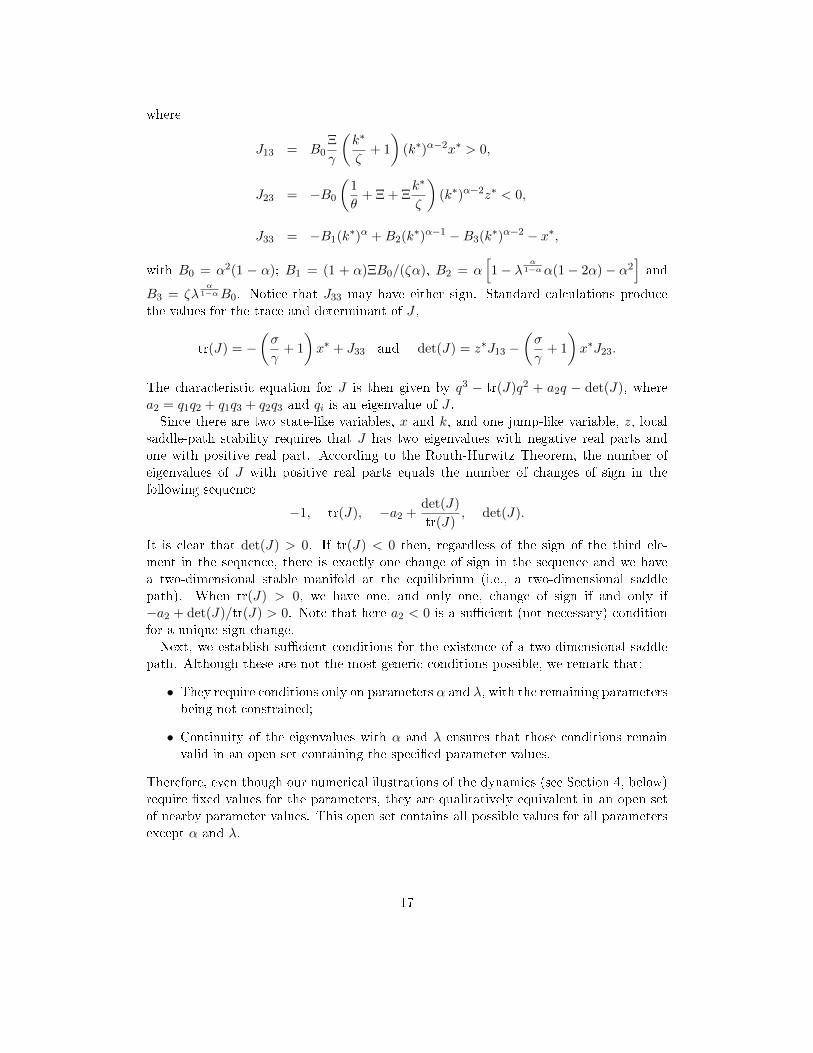
where

J13 = B0Ξ

γ

(k∗

ζ+ 1

)(k∗)α−2x∗ > 0,

J23 = −B0

(1

θ+ Ξ + Ξ

k∗

ζ

)(k∗)α−2z∗ < 0,

J33 = −B1(k∗)α +B2(k∗)α−1 −B3(k∗)α−2 − x∗,

with B0 = α2(1 − α); B1 = (1 + α)ΞB0/(ζα), B2 = α[1− λ α

1−αα(1− 2α)− α2]and

B3 = ζλα

1−αB0. Notice that J33 may have either sign. Standard calculations producethe values for the trace and determinant of J ,

tr(J) = −(σ

γ+ 1

)x∗ + J33 and det(J) = z∗J13 −

(σ

γ+ 1

)x∗J23.

The characteristic equation for J is then given by q3 − tr(J)q2 + a2q − det(J), wherea2 = q1q2 + q1q3 + q2q3 and qi is an eigenvalue of J .Since there are two state-like variables, x and k, and one jump-like variable, z, local

saddle-path stability requires that J has two eigenvalues with negative real parts andone with positive real part. According to the Routh-Hurwitz Theorem, the number ofeigenvalues of J with positive real parts equals the number of changes of sign in thefollowing sequence

−1, tr(J), −a2 +det(J)

tr(J), det(J).

It is clear that det(J) > 0. If tr(J) < 0 then, regardless of the sign of the third ele-ment in the sequence, there is exactly one change of sign in the sequence and we havea two-dimensional stable manifold at the equilibrium (i.e., a two-dimensional saddlepath). When tr(J) > 0, we have one, and only one, change of sign if and only if−a2 + det(J)/tr(J) > 0. Note that here a2 < 0 is a su�cient (not necessary) conditionfor a unique sign change.Next, we establish su�cient conditions for the existence of a two-dimensional saddle

path. Although these are not the most generic conditions possible, we remark that:

• They require conditions only on parameters α and λ, with the remaining parametersbeing not constrained;

• Continuity of the eigenvalues with α and λ ensures that those conditions remainvalid in an open set containing the speci�ed parameter values.

Therefore, even though our numerical ilustrations of the dynamics (see Section 4, below)require �xed values for the parameters, they are qualitatively equivalent in an open setof nearby parameter values. This open set contains all possible values for all parametersexcept α and λ.

17

Furthermore, the condition det(J) > 0, provided the eigenvalues are real, ensureshyperbolicity of the equilibrium. Therefore, a linear approximation of the dynamics isguaranteed to be a good approximation. We use this fact to simplify our subsequentstudy of the dynamics.

Proposition 2. There exists a two-dimensional saddle path in an open set of the param-eter space containing α = 1/3 and such that λ > (92/63)2.

Proof. From tr(J) = − (σ/γ + 1)x∗ + J33 it su�ces to show that

J33 = −B1(k∗)α +B2(k∗)α−1 −B3(k∗)α−2 − x∗ < 0.

The last term is clearly negative so it su�ces to show that the remaining threeterms also add up to a negative number. We note that

−B1(k∗)α +B2(k∗)α−1 −B3(k∗)α−2 < 0⇔ −B3 +B2k∗ −B1k

∗2 < 0.

This occurs trivially when the polynomial of degree two in k∗ has no real roots. Noreal roots appear when

B22 − 4B1B3 < 0.

For α = 1/3, we obtain

B22 − 4B1B3 =

A2

272(−63X2 + 48X + 64), X =

√λ,

which is negative for

X >24 +

√4608

63.

We have24 +

√4608

63<

24 + 68

63=

92

63

and, hence, λ > (92/63)2 ' 2.132 guarantees that tr(J) < 0. �

It follows that, under the above su�cient conditions, the long-run equilibrium is �well-behaved�, meaning that instability, local indeterminacy and limit cycles cannot occur.

4. Transition paths under distinct initial conditions

In order to analyse the transitional dynamics, we perform a numerical illustration. Weconsider the following set of baseline parameter values: γ = 1.2, σ = 1.2, φ = 1,ζ = 3.75, λ = 3, ρ = 0.02, θ = 1.5, α = 1/3, and L = 1. Given that, along the BGP,gQ − gN = (σ + γ)gN , the choice of values for σ and γ is such that (σ + γ) = 2.4, whichis the ratio between the growth rate of the average �rm size and the growth rate of thenumber of �rms we have found in the empirical data.9 The values for λ, θ, ρ and α were

9The data, which are available from the authors upon request, concern 23 European countries in theperiod 1995− 2007 and were taken from the Eurostat online database, at http://epp.eurostat.ec.europa.eu.

18

x∗ k∗ z∗ g∗ µ1 µ2 µ3

0.0074 2.6634 1.1330 0.0252 −0.2064 −0.0192 0.1499

Table 1: Steady-state values of selected endogenous variables and of the eigenvalues(µj , i = 1, 2, 3) for the baseline parameter values.

set in line with the standard growth literature (see, e.g., Barro and Sala-i-Martin, 2004),whereas the normalization of L to unity at every t implies that all aggregate magnitudescan be interpreted as per capita magnitudes. The values of the remaining parameterswere chosen to calibrate the BGP aggregate growth rate around 2.5%/year.For these parameter values, the analytical conditions derived for the existence and

uniqueness of the long-run equilibrium and for the existence of a two-dimensional stablemanifold are veri�ed. The equilibrium is hyperbolic, which garantees that we can makeuse of the Hartman Grobman Theorem to study the dynamics by linearisation. Table1 shows the steady-state values and eigenvalues generated by the baseline parametervalues, which con�rm that the stable manifold results from the existence of two negativereal eigenvalues.

[Table 1 goes about here]

We performed a numerical exercise and concluded that complex eigenvalues, resultingin oscillatory behaviour towards the steady state, are likely to emerge only for implausiblevalues of the parameters. Additionally, in case of oscillatory behaviour it is imperceptibleand does not change the economic interpretation of the transitional dynamics.

Remark. Complex eigenvalues can emerge for di�erent parameter values. For instance,if σ = γ = 0.2 (which are implausibly low values for these parameters) and ζ = 4.6,then the eigenvalues would be:

µ1 = −0.1275 + 0.0576i , µ2 = −0.1275− 0.0576i , µ3 = 0.1426,

with complex eigenvalues associated to the stability. This oscillatory behaviourresults from a change in the entry cost on both margins: a decrease in the extensiveand an increase in the intensive margin, thus illustrating the tension between thehorizontal and vertical barriers to entry.

Because we wish to focus on the behaviour of the state-like variables, x and k, we willabstract from the jump-like variable, z. With that purpose, we follow a similar approachto, e.g., Eicher and Turnovsky (2001) and project the stable space of the linearisedsystem onto the horizontal plane (x, k).10 Thus, henceforth, we are going to consider theprojected dynamics. In the (x, k)-space, the dynamics can be described by the followingsecond-order system

10Since this consists in a non-orthogonal projection, the jump-like variable z continues to have an e�ecton the observed dynamics of x and k.

19

(x

k

)=

µ1v2,2v1,1 − µ2v2,1v1,2

v2,2v1,1 − v2,1v1,2

(µ2 − µ1)v1,2v1,1

v2,2v1,1 − v2,1v1,2(µ1 − µ2)v2,1v2,2

v2,2v1,1 − v2,1v1,2

µ2v2,2v1,1 − µ1v2,1v1,2

v2,2v1,1 − v2,1v1,2

.

(x− x∗k − k∗

),

where µj , i = 1, 2, are the negative eigenvalues and vi,j is the ith element of the eigen-vector associated to µj .From (17)-(18), x can be interpreted either as the growth rate of the number of varieties

(horizontal innovation rate) or, alternatively, as a measure of the intensity of use oftechnological knowledge (or 'technology intensity'), since x is de�ned as a (non-linear)transformation of Q/N , which in turn measures the proportion of the intensive vis-à-visthe extensive component of a given technological-knowledge stock. On the other hand,

recalling (8) and k ≡ K/(L ·Q), we can rewrite the latter as k = (K/Y )1

1−α ; thus, thisvariable can be interpreted as a (non-linear) measure of the physical capital-output ratio.Figure 2 illustrates the projection of the phase diagram (originally on the stable space)

onto the plane (x, k). The stable space is Es = Eµ1 + Eµ2 where:

Eµ1 = {(x(t), k(t)) : k(t)− k∗ =v2,1

v1,1(x(t)− x∗)},

Eµ2 = {(x(t), k(t)) : k(t)− k∗ =v2,2

v1,2(x(t)− x∗)},

and Eµ1 and Eµ2 divide the phase diagram in the phases A, B, C and D. Additionally,we divide phase A and B into two separate regions (by the dashed vertical line), sincethey represent di�erent economic scenarios. The regions to the left (right) of the verticalline can be seen as scenarios where the initial intensity of use of technological knowledge,x(0), is relatively small (large) whereas the regions above (below) Eµ2 represent scenariosof relatively large (small) physical capital-ouput ratio, k(0). Various transition pathsare illustrated in colours, indicating the distinct possibilities of convergence. These arequalitatively di�erent according to the region to which the set of initial conditions belongsin the plane (x, k). If we start in region C or D, both the capital-output ratio and thetechnology-intensity variable converge monotonically, which implies also a monotonicbehaviour of the economic growth rate, as we will see below. If we start in any otherregion, both state-like variables have a non-monotonic transition that transmits to theeconomic growth rate.11

[Figure 2 goes about here]

We seek to provide economic interpretation for the dynamics of the state-like variables,x and k, and other key variables of interest such as: the vertical innovation rate, I(t); the

11The transitions in regions A2 and B2 are qualitatively identical to the ones in A1 and B1, respectively.Therefore, in what follows, we are only interested in explicitly analysing the transitional dynamics inregions A1, B1, C and D.

20

5.5 6 6.5 7 7.5 8 8.5 9

x 10−3

2.3

2.4

2.5

2.6

2.7

2.8

2.9

x(t)

k(t)

A1

B1

B2

A2

C

D

Esµ

1

Esµ

2

Figure 2: Projection of the phase diagram onto the plane (x, k). Various possible tran-sitions are illustrated in colours, one for each region. In regions C and D, theconvergence is monotonic, whereas in the other regions the convergence of bothstate-like variables is non monotonic.

economic growth rate, gY (t) = I(t)·Ξ+x(t)+αgk(t) (see (8) and (19)); the technological-knowledge stock, Q(t); the stock of physical capital, K(t); the number of �rms/varieties,N(t); average �rm size, K(t)/N(t); and the saving rate, s(t) = 1 − z(t)/k(t)α.Someof these variables (Q, K, N , and K/N) are non stationary in the long run and, thus,for convenience, we will represent them after being adjusted for the respective timetrend: Qd(t) = Q(t) · e−g∗Qt; Kd(t) = K(t) · e−g∗Kt; Nd(t) = N(t) · e−g∗N t ; (K/N)d(t) =Kd(t)/Nd(t). We are also interested in the time-path of the speed of convergence ofx and k, computed as ω(t) = −y(t)/ (y(t)− y∗), where y∗ is the steady-state value ofy ∈ {x, k}(see, e.g., Eicher and Turnovsky, 2001).The initial conditions considered for each one of the di�erent regions are such that

the vertical innovation rate and the number of varieties are positive throughout thetransition, while the linearisation holds as a good approximation for the dynamics.12

In order to relate our results with the empirical evidence on transition economies, wewill focus on the case of economies all of which exhibit an initial per capita output,Y (0)/L = Q(0)1−α[K(0)/L]α, below that of the frontier countries,13 but yet may featuredistinct combinations of Q(0), K(0) and N(0) (and hence of k(0) and x(0), as referredto above).The economic interpretation of the mechanism underlying the transitional path is as

12We arbitrarely consider Q(0) = 1 and then compute K(0) and N(0) by the respective relationshipwith Q(0).

13We also assume that both Q(0) and K(0)/L are below the frontier levels.

21

follows, analysed counter-clockwise through the relevant regions of Figure 2.

Region A1 The initial conditions are such that k∗ < k(0) and x∗ < x(0). This would bethe case of an economy characterised by relatively large initial capital-output ratio andintensity of use of technological knowledge/horizontal innovation rate. The adjustmentof the economy towards the steady state is characterised by several variables followingnon-monotonic transition paths (see Figure 3).The initial increase in x is justi�ed by the complementarity between the two types of

innovation, i.e., the initially high value of the vertical innovation rate, I, generates anincrease in the technological-knowledge stock, Q, that stimulates horizontal innovation(see (18)). However, this e�ect is dampened by the rise of the horizontal entry cost, η,driven by the rapid increase in the number of varieties, N , itself a result of the largeinitial x. Eventually, the rise of η dominates and x follows a downward path convergingto the steady state. This non-monotonic behavior is re�ected in the dynamics of thecorresponding speed of convergence, ωx. Observe that the high initial I results from theexisting complementarity between the capital-output ratio and the intensive margin ofinnovation: a larger k induces a larger pro�t per �rm (see (5)), which generates an higherincentive to vertical innovation by rising the e�ective rate of return, r + I (see (11)).The physical capital-output ratio, k, is initially high and rapidly decreasing due to the

low marginal productivity of physical capital, K, and the relatively large pro�tabilityof innovation activities. However, over time, the reduction in the horizontal innovationrate frees resources for the accumulation of K; eventually, the former e�ect is morethan compensated by the latter and k rises towards the steady state. Thus, the observedundershooting of k mirrors the hump-shaped trajectory of the horizontal innovation rate,x. The speed of convergence, ωk, re�ects the non-monotonic transition of k, in particularthe undershooting, which implies an in�nite speed of convergence at that point. Thevertical innovation rate, I, follows a similar path to k, as a consequence of the referredto complementarity between physical capital accumulation and the intensive margin ofinnovation.The number of varieties, N , grows over transition at a greater rate than in the BGP

(given that x(t) > x∗ for every �nite t) and, thus, the detrended number of varieties, Nd,increases towards the steady state. In contrast, physical capital, K, starts by growingless than in the BGP but eventually accelerates to grow above the BGP � but by lessthan N , since the negative or very small positive gk puts a drag on the overall growthrate of K (recall that K grows at the rate gk + gQ). Thus, detrended physical capital,Kd, observes a slight fall in the �rst stage of its transition path and then increases butat a slow rate towards the steady state.14 This leads to a monotonic convex downwardpath of the detrended �rm size, (K/N)d.The saving rate, s, begins by rising dramatically as the resources are re-allocated to

horizontal R&D and while vertical R&D (re�ecting the vertical innovation rate, I) isstill high. It experiences a slight overshoot after which it starts falling as the decline ofresources devoted to horizontal R&D more than compensates �rst for the recovery of the

14Since this is a very moderate e�ect, it is not noticeable in the K panel in Figure 3.

22

physical capital accumulation rate, gk, and then for the increase in vertical R&D due tothe recovery of I.Finally, the economic growth rate, gY , is initially low, because gk is negative, but

experiences a non-monotonic, hump-shaped, transition. As gk becomes less negative,the horizontal innovation rate, x, increases and the vertical innovation rate, I, is stillhigh (although falling), gY observes a notorious increase and overshoots. However, theensuing decline of x and gk outweights the recovery of I and generates a gradual downwardmovement of gY towards the long-run equilibrium.

[Figure 3 goes about here]

23

Figura 3: Transitional dynamics of the key economic variables and of the speeds of con-vergence of k and x (ωk and ωx) for an economy that sets o� with k∗ < k(0)and x∗ < x(0) (region A1 of Figure 2). The economic growth rate, gY , andthe saving rate, s, display a hump-shaped behaviour, while detrended �rm size,(K/N)d, decreases monotonically.

24

Region D Now, we turn to the case of an economy with a relatively large initialcapital-output ratio, but a relatively small initial intensity of use of technological knowl-edge/horizontal innovation rate. The initial conditions in region D satisfy15

x(0) < x∗ ∧ v2,2

v1,2(x(t)− x∗) + k∗ < k(0) <

v2,1

v1,1(x(t)− x∗) + k∗.

As depicted by Figure 4, the transition is quite distinct from the one originating in regionA1, with the predominance of monotonic transition paths.Along the whole transition path, x increases commanded by the increase in the technological-

knowledge stock, Q, which has an o�seting e�ect on the horizontal entry costs, η. Thishappens because the initial low x determines a slow increase in the number of varieties,N , and hence a slow increase in η, whereas the large initial vertical innovation rate, I,stimulates a rapid growth of Q.The capital-output ratio, k, which is initially high, decreases monotonically comman-

ded by the low marginal productivity of physical capital, K, and the continuous re-allocation of resources to horizontal R&D.In turn, the path of the technological-knowledge stock, Q, shows a very di�erent pat-

tern: as already said, Q rises rapidly during the early stages re�ecting the high initialvertical innovation rate, I, but eventually it starts to increase at a lower rate than in theBGP as I declines monotonically (in turn re�ecting the behaviour of k); as a consequence,the detrended technological-knowledge stock, Qd, follows a hump-shaped path towardsthe steady state. In contrast, the detrended measure of �rm size, (K/N)d, shows aninverted hump-shaped behaviour. Indeed, the number of varieties, N , grows over tran-sition at a smaller rate than in the BGP (re�ecting x(t) < x∗) and, thus, the detrendednumber of varieties, Nd, falls towards the steady state. However, detrended physical ca-pital, Kd, starts by falling by more than Nd, re�ecting the fact that the initially negativegk outweights the positive growth rate of Q; hence, (K/N)d falls and undershoots itslong-run level. Then, as gk recovers and the fall in Kd slows down, the transition-pathis reversed and (K/N)d starts increasing.Lastly, both the economic growth rate, gY , and the saving rate, s, follow a monotonic

upward path towards the steady state driven by the monotonic increase in gk and x.

[Figure 4 goes about here]

15The condition on k(0) guarantees that the economy does not start in regions A2 or B1.

25

Figura 4: Transitional dynamics of the key economic variables and of the speeds of con-vergence of k and x (ωk and ωx) for an economy that sets o� with k∗ < k(0)and x(0) < x∗ (region D of Figure 2). The economic growth rate, gY , andthe saving rate, s, increase monotonically, while detrended �rm size, (K/N)d,displays an inverted hump-shaped behaviour.

26

Region B1 An economy initially in region B1 corresponds to the case of an economywith relatively low initial capital-output ratio, k(0) < k∗, and intensity of use of tech-nological knowledge/horizontal innovation rate, x(0) < x∗. This represents the oppositescenario of an economy starting in region A1 and thus the adjustment paths, namely thenon-monotonic paths of the state-like variables, are a mirror image of those observed inthat region (see Figure 5).The initial low x determines a slow increase in the number of varieties, N , and hence

a slow increase in η. Nevertheless, the also low initial vertical innovation rate, I, impliesan even slower increase in the technological-knowledge stock, Q, and thus x falls in the�rst stage of transition. The recovery of I and the consequent acceleration of Q puts xon an upward path towards the steady state.The physical capital-output ratio, k, is initially low but rapidly increasing, induced by

the high marginal productivity of physical capital, K, and the relatively low pro�tabilityof innovation activities. However, over time, the increase in the horizontal innovationrate deviates resources from the accumulation of K; eventually, the former e�ect is morethan compensated by the latter and k starts a downfall towards the steady state. Thespeed of convergence, ωk, re�ects the non-monotonic transition of k, in particular theobserved overshooting.The number of varieties, N , grows over transition at a smaller rate than in the BGP

(due to x(t) < x∗) and, thus, the detrended number of varieties, Nd, falls towards thesteady state. In contrast, physical capital, K, starts by growing more than in the BGP(re�ecting an initially large positive gk) but eventually slows down to grow below theBGP; thus, detrended physical capital, Kd, observes a hump-shaped behaviour, whichdetermines a monotonic concave upward path of detrended �rm size, (K/N)d.The saving rate, s, begins by falling dramatically as the investment in horizontal R&D

decreases and while vertical R&D (re�ecting the vertical innovation rate, I) is still low.It experiences a slight undershoot after which it starts increasing as the allocation ofresources to horizontal R&D more than compensates �rst the fall of the physical capitalaccumulation rate, gk, and then the reduction in vertical R&D due to the falling I.Finally, the nonlinear adjustment of the state-like variables leads once again to a

nonlinear transition of the economic growth rate, gY . In contrast with region A1, theeconomic growth rate, gY , is initially high, because gk is large positive, and experiences aninverted hump-shaped transition. As gk and the horizontal innovation rate, x, decreaseand the vertical innovation rate, I, is still low (although increasing), gY decreases rapidlyand undershoots. However, the ensuing recovery of x and gk outweights the decrease inI and allows for a gradual upward movement of gY towards the long-run equilibrium.

[Figure 5 goes about here]

27

Figura 5: Transitional dynamics of the key economic variables and of the speeds of con-vergence of k and x (ωk and ωx) for an economy that sets o� with k(0) < k∗

and x(0) < x∗ (region B1 of Figure 2). The economic growth rate, gY , and thesaving rate, s, display an inverted hump-shaped behaviour, while detrended�rm size, (K/N)d, increases monotonically.

28

Region C Finally, the scenario of an economy initially with relatively low physicalcapital-output ratio, but a relatively large intensity of use of technological knowledge/horizontalinnovation rate corresponds to an economy in region C. Initial conditions in this regionsatisfy16

x∗ < x(0) ∧ v2,1

v1,1(x(t)− x∗) + k∗ < k(0) <

v2,2

v1,2(x(t)− x∗) + k∗.

Most aspects of the transition are a mirror image of those pertaining to region D (seeFigure 6).The monotonic decline of x towards the steady state re�ects the e�ect of the horizontal

entry costs along the whole transition path. The initial high x determines a fast increasein the number of varieties, N , and hence a fast increase in η, whereas the low initialvertical innovation rate, I, implies a slow growth of Q.The capital-output ratio, k, which is initially low, increases monotonically commanded

by the high marginal productivity of physical capital, K, and the continuous re-allocationof resources from horizontal R&D to physical investment.The technological-knowledge stock, Q, �rst diverges from the BGP due to the initi-

ally low vertical inovation rate, I, but the ensuing increase in I boosts Q such that thetransition is reversed; thus, in detrended terms, this variable follows an inverted hump-shaped path. In contrast, detrended �rm size, (K/N)d, shows a hump-shaped behaviour.Initially K/N grows above the BGP rate because the large positive gk more than com-pensates for the low growth of Q and the high x (which propels N). As the increase ofgk is dampened and the innovation rate on both margins decrease (x and I), the growthrate of K/N declines towards the BGP level.At last, both the economic growth rate, gY , and the saving rate, s, follow a monotonic

downward path driven by the monotonic decrease in gk and x.

[Figure 6 goes about here]

16The condition on k(0) guarantees that the economy does not start in regions B2 or A1.

29

Figura 6: Transitional dynamics of the key economic variables and of the speeds of con-vergence of k and x (ωk and ωx) for an economy that sets o� with k(0) < k∗

and x∗ < x(0) (region C of Figure 2). The economic growth rate, gY , andthe saving rate, s, decrease monotonically, while detrended �rm size, (K/N)d,displays a hump-shaped behaviour.

30

5. Discussion and concluding remarks

Historical evidence of the stages of development of the nowadays most developed countriesseems to suggest monotonic transitional dynamics (e.g., Maddison, 2001). However, if onelooks at the development experience of a number of countries in the postwar period, thedata suggests non-monotonic behaviour, through hump-shaped or inverted hump-shapedtransitions (e.g., Fiaschi and Lavezzi, 2003a, 2007). Our paper develops an endogenousgrowth model of physical capital accumulation and two types of lab-equipment R&Dfeaturing an analytical mechanism that encompasses all these cases.Under this setup, both the intensive and extensive margins of growth are fully en-

dogenous, in contrast with the existent models of the knowledge-driven type. We studiedanalytically the long-run equilibrium stability and transitional dynamics properties of themodel, and established su�cient conditions for saddle-path stability. These conditionsimpose constraints only on two structural parameters, whereas the continuity propertyof the eigenvalues ensures that those conditions remain valid in an open set containingthe speci�ed values for these parameters.As an alternative to the hypothesis of multiple equilibria and 'poverty traps' (e.g.,

Ciccone and Matsuyama, 1996; Fiaschi and Lavezzi, 2003a, 2007), our model allows usto address the above empirical evidence by emphasising the role played by an economy'sinitial conditions in de�ning the shape of its transition path towards the (unique) long-run equilibrium. We �nd that distinct initial physical capital-output ratios and/or initialtechnology intensities in otherwise similar economies may imply contrasting � eithermonotonic or non-monotonic � convergence paths of key economic variables, namely theeconomic growth rate, saving rate, and �rm size (assets per �rm), as emphasised by theempirical literature.In particular regarding the transition of growth rates, the evidence reported by Mad-

dison (2001) (monotonic downward transition) corresponds, in our model, to the case ofthe economies with initial below-the-frontier per capita output and that start in regionC of the phase diagram, characterised by an initial relative scarcity of physical inputs �i.e., of physical capital, but also of varieties of technological goods (implying a relativelyhigh technology intensity). Therefore, our model specialises the explanation proposed bythe neoclassical growth model for this sort of transition, only focused on physical capital.The evidence found by Fiaschi and Lavezzi (2003a, 2007) for initially 'low' and 'middle-low' income countries (respectively, inverted hump-shaped and hump-shaped transitions)corresponds, in the model, to the case of the economies also with initial below-the-frontierper capita output but that start, respectively, in regions B1 and A1 of the phase dia-gram. In the former case, the economies are characterised by an initial relative scarcityof physical capital but a relative abundance of varieties of technological goods (implyinga relatively low technology intensity). These initial conditions determine a �rst phase ofhigh growth (take-o�), as in the neoclassical growth model, but which is followed by aphase of quite lower growth rates (i.e., an undershooting phase, which, if long-lasting,may be perceived as a 'poverty trap') and, eventually, by a slow recovery into a regime ofmoderate growth. In the other case (region A1), the opposite occurs: initial conditionsfavour the exploration of the complementarity between physical capital and technology

31

intensity, and thus a transition occurs in which growth rates do not peak at the beginningof the convergence process but later on; hence, the overshooting of the growth rate, laterfollowed by a slowdown towards a regime of moderate growth.The model also predicts speeds of convergence that vary over time and across vari-

ables, in particular with physical capital and knowledge displaying contrasting speeds ofconvergence, in line with the empirical evidence emphasised by, e.g., Bernard and Jones(1996).Our theoretical model allows for technological-knowledge and physical capital accu-

mulation, but no human capital accumulation. However, since, in our model, verticaland horizontal R&D are complementary, a possible extension is to replace vertical R&Dwith human capital accumulation, in order to explore the complementarity between hu-man capital and technology accumulation, in line with Nelson and Phelps (1966), Arnold(1998), Kosempel (2004), and others. Then, our equation (18) implies that the growthrate of the number of varieties (i.e., the rate of technology accumulation in this versionof the model) is a positive function of the stock of human capital, whereas reinterpretingequation (19) as a human-capital accumulation function implies that the accumulation ofhuman capital is a negative function of the existing number of varieties (i.e., the technol-ogy stock in this version of the model). The idea here is that a higher technology stockmakes learning more complex and demanding, in line with, e.g., Galor and Moav (2002)and Reis and Sequeira (2007). This modi�cation to our model shows that technologyintensity is isomorphic to the human capital-technology stock ratio and, thus, a country'sinitial conditions can alternatively be interpreted in terms of the physical capital-outputand the human capital-technology stock ratios.Overall, these results suggest that institutions may be relevant for a country's growth

experience also by playing a role in the determination of the initial endowment of physicalversus immaterial inputs: on one hand, physical capital versus technological-knowledgestock; on the other, the proportion of the extensive versus the intensive (or human-capital) component of a given technological-knowledge stock. In this context, not onlymay institutions be capable of in�uencing the timing of the economies' take-o� (see, e.g.,Jones and Romer, 2010), but also the characteristics of their transition (speed and shape)towards the respective long-run equilibrium.

References

Aghion, P., and P. Howitt (1992): �A Model of Growth Through Creative Destruc-tion,� Econometrica, 60(2), 323�351.

Arnold, L. (2000): �Endogenous Technological Change: a Note on Stability,� EconomicTheory, 16, 219�226.

(2006): �The Dynamics of the Jones R&D Growth Model,� Review of Economic

Dynamics, 9, 143�152.

Arnold, L. G. (1998): �Growth, Welfare, and Trade in an Integrated Model of Human-Capital Accumulation and Research,� Journal of Macroeconomics, 20 (1), 81�105.

32

Arnold, L. G., and W. Kornprobst (2008): �Comparative Statics and Dynamics ofthe Romer R&D Growth Model with Quality Upgrading,� Macroeconomic Dynamics,12, 702�716.

Barro, R., and X. Sala-i-Martin (2004): Economic Growth. Cambridge, Mas-sachusetts: MIT Press, second edn.

Bernard, A. B., and C. I. Jones (1996): �Technology and Convergence,� EconomicJournal, 106, 1037�1044.

Brito, P., and H. Dixon (2009): �Entry and the Accumulation of Capital: a TwoState-Variable Extension to the Ramsey Model,� International Journal of Economic

Theory, 5, 333�357.

(2013): �Fiscal Policy, Entry and Capital Accumulation: Hump-Shaped Re-sponses,� Journal of Economic Dynamics & Control, 37, 2123�2155.

Ciccone, A., and K. Matsuyama (1996): �Start-up costs and pecuniary externalitiesas barriers to economic development,� Journal of Development Economics, 49, 33�59.

Dinopoulos, E., and P. Thompson (1998): �Schumpeterian Growth Without ScaleE�ects,� Journal of Economic Growth, 3 (December), 313�335.

(2000): �Endogenous Growth in a Cross-Section of Countries,� Journal of In-ternational Economics, 51, 335�362.

Eicher, T., and S. Turnovsky (2001): �Transitional Dynamics in a Two-Sector Non-Scale Growth Model,� Journal of Economic Dynamics and Control, 25, 85�113.

Etro, F. (2008): �Growth Leaders,� Journal of Macroeconomics, 30, 1148�1172.

Evans, G. W., S. M. Honkapohja, and P. Romer (1998): �Growth Cycles,� Amer-ican Economic Review, 88, 495�515.

Fiaschi, D., and A. M. Lavezzi (2003a): �Distribution Dynamics and NonlinearGrowth,� Journal of Economic Growth, 8, 379�401.

Fiaschi, D., and A. M. Lavezzi (2003b): �Nonlinear Economic Growth: Some The-ory and Cross-Country Evidence,� Discussion Papers, Dipartimento di Economia e

Management (DEM), University of Pisa, 14, 1�40.

(2007): �Nonlinear Economic Growth: Some Theory and Cross-Country Evi-dence,� Journal of Development Economics, 84, 271�290.

Galor, O., and O. Moav (2002): �Natural Selection and the Origin of EconomicGrowth,� Quartely Journal of Economics, 117, 1133�1191.

Geroski, P. (1995): �What Do We Know About Entry?,� International Journal of

Industrial Organization, 13, 421�440.

33

Gil, P. M. (2010): �Stylised Facts and Other Empirical Evidence on Firm Dynamics,Business Cycle and Growth,� Research in Economics, 64, 73�80.

Gil, P. M., P. Brito, and O. Afonso (2013): �Growth and Firm Dynamics withHorizontal and Vertical R&D,� Macroeconomic Dynamics, 17 (7), 1438�1466.

Gómez, M. (2005): �Transitional Dynamics in an Endogenous Growth Model with Phys-ical Capital, Human Capital and R&D,� Studies in Nonlinear Dynamics & Economet-

rics, 9(1), Article 5.

Growiec, J., and I. Schumacher (2013): �Technological Opportunity, Long-RunGrowth, and Convergence,� Oxford Economic Papers, 65, 323�351.

Howitt, P. (1999): �Steady Endogenous Growth with Population and R&D InputsGrowing,� Journal of Political Economy, 107(4), 715�730.

(2002): �Endogenous Growth and Cross-Country Income Di�erences,� AmericanEconomic Review, 90(4), 829�846.

Howitt, P., and P. Aghion (1998): �Capital Accumulation and Innovation as Com-plementary Factors in Long-Run Growth,� Journal of Economic Growth, 3, 111�130.

Jones, C. (1995): �R&D Based Models of Economic Growth,� Journal of Political Econ-omy, 103, 759�784.

Jones, C. I., and P. M. Romer (2010): �The New Kaldor Facts: Ideas, Institutions,Population, and Human Capital,� American Economic Journal: Macroeconomics, 2(1),224�245.

Jones, C. I., and J. C. Williams (2000): �Too Much of a Good Thing? The Economicsof Investment in R&D,� Journal of Economic Growth, 5, 65�85.

Kosempel, S. (2004): �A Theory of Development and Long Run Growth,� Journal ofDevelopment Economics, 75, 201�220.

Loyaza, N., K. Schmidt-Hebbel, and L. Serven (2000): �Saving in DevelopingCountries: An Overview,� World Bank Economic Review, 14, 393�414.

Maddison, A. (1992): �A Long-Run Perspective on Saving,� Scandinavian Journal of

Economics, 94(2), 181�196.

(2001): The World Economy, a Millenial Perspective. Paris: OECD Develop-ment Center Studies.

Nelson, R. R., and E. S. Phelps (1966): �Investment in Humans, TechnologicalDi�usion, and Economic Growth,� American Economic Review, 56(1/2), 69�75.

Papageorgiou, C., and F. Perez-Sebastian (2006): �Dynamics in a Non-Scale R&DGrowth Model with Human Capital: Explaining the Japanese and South Korean De-velopment Experiences,� Journal of Economic Dynamics and Control, 30, 901�930.

34

Peretto, P. (1998): �Technological Change and Population Growth,� Journal of Eco-nomic Growth, 3 (December), 283�311.

Reis, A. B., and T. N. Sequeira (2007): �Human Capital and Overinvestment inR&D,� Scandinavian Journal of Economics, 109(3), 573�591.

Rivera-Batiz, L., and P. Romer (1991): �Economic Integration and EndogenousGrowth,� Quarterly Journal of Economics, 106 (2), 531�555.

Romer, P. M. (1990): �Endogenous Technological Change,� Journal of Political Econ-omy, 98(5), 71�102.

Sedgley, N., and B. Elmslie (2013): �The Dynamic Properties of Endogenous GrowthModels,� Macroeconomic Dynamics, forthcoming, doi:10.1017/S1365100512000119.

Sequeira, T. (2011): �R&D Spillovers in an Endogenous Growth Model with PhysicalCapital, Human Capital, and Varieties,� Macroeconomic Dynamics, 15, 223�239.

Sequeira, T., A. F. Lopes, and O. Gomes (2014): �A Growth Model with Quali-ties, Varieties, and Human Capital: Stability and Transitional Dynamics,� Studies inNonlinear Dynamics & Econometrics, 18(5), 543�555.

Strulik, H. (2007): �Too Much of a Good Thing? The Quantitative Economics ofR&D-driven Growth Revisited,� Scandinavian Journal of Economics, 109 (2), 369�386.

Strulik, H., K. Prettner, and A. Prskawetz (2013): �The Past and Future ofKnowledge-Based Growth,� Journal of Economic Growth, 18, 411�437.

Zeng, J. (2003): �Reexamining the Interaction Between Innovation and Capital Accu-mulation,� Journal of Macroeconomics, 25, 541�560.

Appendix

A. General equilibrium: derivation of equation (24)

Consider the households' balance sheet

a(t) = K(t) + η(t) ·N(t) (39)

Hence, we can characterise the change in the value of equity as

a(t) = K(t) + η(t) ·N(t) + η(t) · N(t) (40)

Substitute (21) in the left-hand side of (40) and ηη = Q

Q − NN = I ·

(λ

α1−α − 1

)� derived

from (16) and (19) � in the right-hand side, to get

35

(r(t) + I(t)) · η(t) ·N(t)− I(t) · η(t) ·N(t) + r(t) ·K(t(t)) + w(t) · L− C(t) =

= K(t) + I(t) ·(λ

α1−α − 1

)· η(t) ·N(t) + η(t) · N(t) (41)

Since the real interest rate r consists of dividend payments in units of asset price minusthe Poisson death rate, i.e., r = π

V − I, for each t, then π · N = (r + I) · V · N .Furthermore, it is easy to show, bearing in mind (1), (4) and (6), that w ·L = (1−α) ·Y ,Π = π ·N = (α− α2) · Y and r ·K = α2 · Y . Using these results in (41), yields

(α− α2) · Y (t) + α2 · Y (t) + (1− α) · Y (t)− C(t) =

= K(t) +[I(t) + I(t) ·

(λ

α1−α − 1

)]· η(t) ·N(t) + η(t) · N(t) (42)

Next, recall that Rn = ηN and Rv = λα

1−α · ζ · L · I ·Q, such that (42) reads as (24) inthe text.

36