Embed Size (px)
Citation preview
Technical ReportTTIC-TR-2009-2
May 2009
CEAL: A C-Based Language for Self-AdjustingComputation
Matthew A. HammerToyota Technological Institute at [email protected]
Umut A. AcarToyota Technological Institute at [email protected]
Yan ChenToyota Technological Institute at [email protected]

ABSTRACT
Self-adjusting computation offers a language-centric approach to writing programs that can automaticallyrespond to modifications to their data (e.g., inputs). Except for several domain-specific implementations,however, all previous implementations of self-adjusting computation assume mostly functional, higher-orderlanguages such as Standard ML. Prior to this work, it was not known if self-adjusting computation canbe made to work with low-level, imperative languages such as C without placing undue burden on theprogrammer.
We describe the design and implementation of CEAL: a C-based language for self-adjusting computation.The language is fully general and extends C with a small number of primitives to enable writing self-adjustingprograms in a style similar to conventional C programs. We present efficient compilation techniques fortranslating CEAL programs into C that can be compiled with existing C compilers using primitives suppliedby a run-time library for self-adjusting computation. We implement the proposed compiler and evaluate itseffectiveness. Our experiments show that CEAL is effective in practice: compiled self-adjusting programsrespond to small modifications to their data by orders of magnitude faster than recomputing from scratchwhile slowing down a from-scratch run by a moderate constant factor. Compared to previous work, wemeasure significant space and time improvements.

1 Introduction
Researchers have long observed that in many applications, application data evolves slowly or incrementallyover time, often requiring only small modifications to the output. This creates the potential for applicationsto adapt to changing data significantly faster than recomputing from scratch. To realize this potential,researchers in the algorithms community develop so called dynamic or kinetic algorithms or data structuresthat take advantage of the particular properties of the considered problem to update computations quickly.Such algorithms have been studied extensively over a range of hundreds of papers (e.g. [13, 17] for surveys).These advances show that computations can often respond to small modifications to their data nearly a linearfactor faster than recomputing from scratch, in practice delivering speedups of orders of magnitude. As aframe of comparison, note that asymptotic improvements in performance far surpasses the goal of parallelism,where speedups are bound by the number of available processors. Designing, analyzing, and implementingdynamic/kinetic algorithms, however, can be complex even for problems that are relatively simple in theconventional setting, e.g., the problem of incremental planar convex hulls, whose conventional version isstraightforward, has been studied over two decades (e.g., [31, 11]). Due to their complexity, implementingthese algorithms is an error-prone task that is further complicated by their lack of composability.
Self-adjusting computation (e.g., [4, 3]) offers a language-centric approach to realizing the potentialspeedups offered by incremental modifications. The approach aims to make writing self-adjusting programs,which can automatically respond to modifications to their data, nearly as simple as writing conventionalprograms that operate on unchanging data, while delivering efficient performance by providing an automaticupdate mechanism called change propagation. In self-adjusting computation, programs are stratified into twocomponents: a meta-level mutator and a core. The mutator interacts with the user or the outside world andinterprets and reflects the modifications in the data to the core. The core, written like a conventional program,takes some input and produces an output. The core is self-adjusting: it can respond to modifications to itsdata by employing a general-purpose, built-in change propagation mechanism. The mutator can execute thecore with some input from scratch, which we call a from-scratch or an initial run, modify the data of thecore, including the inputs and other computation data, and update the core by invoking change propagation.A typical mutator starts by performing a from-scratch run of the program (hence the name initial run), andthen repeatedly modifies the data and updates the core via change propagation.
At a high level, change propagation updates the computation by re-executing the parts that are affectedby the modifications, while leaving the unaffected parts intact. Change propagation is guaranteed to updatethe computation correctly: the output obtained via change propagation is the same as the output of afrom-scratch execution with the modified data. Even in the worst case, change propagation falls back to afrom-scratch execution—asymptotically, it is never slower (in an amortized sense)—but it is often significantlyfaster than re-computing from-scratch.
Previous research developed language techniques for self-adjusting computation and applied it to a num-ber of application domains (e.g., for a brief overview [3]). The applications show that from-scratch executionsof self-adjusting programs incur a moderate overhead compared to conventional programs but can respondto small modifications orders-of-magnitude faster than recomputing from scratch. The experimental evalua-tions show that in some cases self-adjusting programs can be nearly as efficient as the “hand-designed” andoptimized dynamic/kinetic algorithms (e.g., [6]). Recent results also show that the approach can help de-velop efficient solutions to challenging problems such as some three-dimensional motion simulation problemsthat have resisted algorithmic approaches [5].
Existing general-purpose implementations of self-adjusting computation, however, are all in high-level,mostly functional languages such as Standard ML (SML) or Haskell [26, 12]. Several exist in lower-level lan-guages such as C [6] and Java [34] but they are domain-specific. In Shankar and Bodik’s implementation [34],which targets invariant-checking applications, core programs must be purely functional and functions cannotreturn arbitrary values or use values returned by other functions in an unrestricted way.
Acar et al’s C implementation [6] targets a domain of tree applications. Neither approach offers ageneral-purpose programming model. The most general implementation is Hammer et al’s C library [21],whose primary purpose is to support efficient memory management for self-adjusting computation. The Clibrary requires core programs to be written in a style that makes dependencies between program data andfunctions explicit, limiting its effectiveness as a source-level language.
1

That there is no general-purpose support for self-adjusting computation in low level, imperative languagessuch as C is not accidental: self-adjusting computation critically relies on higher-order features of high-levellanguages. To perform updates efficiently, change propagation must be able to re-execute a previously-executed piece of code in the same state (modulo the modifications), and skip over parts of the computationthat are unaffected by the modifications. Self-adjusting computation achieves this by representing the depen-dencies between the data and the program code as a trace that records specific components of the programcode and their run-time environments. Since higher-order languages can natively represent closed functions,or closures, consisting of a function and its free variables, they are naturally suitable for implementing traces.Given a modification, change propagation finds the closures in the trace that depend on the modified data,and re-executes them to update the computation and the output. Change propagation utilizes recordedcontrol dependencies between closures to identify the parts of the computation that need to be purged anduses memoization to recover the parts that remain the same. To ensure efficient change propagation, thetrace is represented in the form of a dynamic dependence graph that supports fast random access to theparts of the computation to be updated.
In this paper, we describe the design, implementation, and evaluation of CEAL: a C-based language forself-adjusting computation. The language extends C with several primitives for self-adjusting computation(Section 2). Reflecting the structure of self-adjusting programs, CEAL consists of a meta language for writingmutators and a core language for writing core programs. The key linguistic notion in both the meta andthe core languages is that of the modifiable reference or modifiable for short. A modifiable is a location inmemory whose contents may be read and updated. CEAL offers primitives to create, read (access), andwrite (update) modifiables just like conventional pointers. The crucial difference is that CEAL programs canrespond to modifications to modifiables automatically. Intuitively, modifiables mark the computation datathat can change over time, making it possible to track dependencies selectively. At a high level, CEAL canbe viewed as a dialect of C that replaces conventional pointers with modifiables.
By designing the CEAL language to be close to C, we make it possible to use familiar C syntax to writeself-adjusting programs. This poses a compilation challenge: compiling CEAL programs to self-adjustingprograms requires identifying the dependence information needed for change propagation. To address thischallenge, we describe a two-phase compilation technique (Sections 5 and 6). The first phase normalizes theCEAL program to make the dependencies between data and parts of the program code explicit. The secondphase translates the normalized CEAL code to C by using primitives supplied by a run-time-system (RTS)in place of CEAL’s primitives. This requires creating closures for representing dependencies and efficientlysupporting tail calls. We prove that the size of the compiled C code is no more than a multiplicative factorlarger than the source CEAL program, where the multiplicative factor is determined by the maximum numberof live variables over all program points. The time for compilation is bounded by the size of the compiled Ccode and the time for live variable analysis. Section 3.2 gives an overview of the compilation phases via anexample.
We implement the proposed compilation technique and evaluate its effectiveness. Our compiler, cealc,provides an implementation of the two-level compilation strategy and relies on the RTS for supplying the self-adjusting-computation primitives. Our implementation of the RTS employs the recently-proposed memorymanagement techniques [21], and uses asymptotically optimal algorithms and data structures to supporttraces and change propagation. For practical efficiency, the compiler uses intra-procedural compilationtechniques that make it possible to use simpler, practically efficient algorithms.
We perform an experimental evaluation by considering a range of benchmarks, including several primitiveson lists (e.g., map, filter), several sorting algorithms, and computational geometry algorithms for computingconvex hulls, the distance between convex objects, and the diameter of a point set. As a more complexbenchmark, we implement a self-adjusting version of the Miller-Reif tree-contraction algorithm, which is ageneral-purpose technique for computing various properties of trees (e.g., [27, 28]). Our experiments showthat our compiler is between a factor of 3–8 slower and generates binaries that are 2–5 times larger than gcc.Our timing measurements show that CEAL programs are about 6–19 times slower than the correspondingconventional C program when executed from scratch, but can respond to small changes to their data orders-of-magnitude faster than recomputing from scratch. Compared to the state-of-the-art implementation of
2

self-adjusting computation in SML [26], CEAL uses about 3–5 times less memory. In terms of run time,CEAL performs significantly faster than the SML-based implementation. In particular, when the SMLbenchmarks are given significantly more memory than they need, we measure that they are about a factorof 9 slower. Moreover, this slowdown increases (without bound) as memory becomes more limited. We alsocompared our implementation to a hand-optimized implementation of self-adjusting computation for treecontraction [6]. Our experiments show that we are about 3–4 times slower.
In this paper, we present a C-based general-purpose language for self-adjusting computation. Our con-tributions include the language, the compiler, and the experimental evaluation.
2 The CEAL language
We present an overview of the CEAL language, whose core is formalized in Section 4. The key notion inCEAL is that of a modifiable reference (or modifiable, for short). A modifiable is a location in memory whosecontent may be read and updated. From an operational perspective, a modifiable is just like an ordinarypointer in memory. The major difference is that CEAL programs are sensitive to modifications of the contentsof modifiables performed by the mutator, i.e., if the contents are modified, then the computation can respondto that change by updating its output automatically via change propagation.
Reflecting the two-level (core and meta) structure of the model, the CEAL language consists of twosub-languages: meta and core. The meta language offers primitives for performing an initial run, modifyingcomputation data, and performing change propagation—the mutator is written in the meta language. CEAL’score language offers primitives for writing core programs. A CEAL program consists of a set of functions,divided into core and meta functions: the core functions (written in the core language), are marked with thekeyword ceal, meta functions (written in the meta language) use conventional C syntax. We refer to thepart of a program consisting of the core (meta) functions simply as the core (meta or mutator).
To provide scalable efficiency and improve usability, CEAL provides its own memory manager. Thememory manager performs automatic garbage collection of allocations performed in the core (via CEAL’sallocator) but not in the mutator. The language does not require the programmer to use the providedmemory manager, the programmer can manage memory explicitly if so desired.
The Core Language. The core language extends C with modifiables, which are objects that consist ofword-sized values (their contents) and supports the following primitive operations, which essentially allowthe programmer to treat modifiables like ordinary pointers in memory.
modref t* modref(): creates a(n) (empty) modifiable
void write(modref t *m, void *p): writes p into m
void* read(modref t *m): returns the contents of m
In addition to operations on modifiables, CEAL provides the alloc primitive for memory allocation.For correctness of change propagation, core functions must modify the heap only through modifiables, i.e.,memory accessed within the core, excluding modifiables and local variables, must be write-once. Alsoby definition, core functions return ceal (nothing). Since modifiables can be written arbitrarily, theserestrictions cause no loss of generality or undue burden on the programmer.
The Meta Language. The meta language also provides primitives for operating on modifiables; modrefallocates and returns a modifiable, and the following primitives can be used to access and update modifiables:
void* deref(modref t *m): returns the contents of m.
void modify(modref t *m, void *p): modifies the contents of the modifiable m to contain p.
As in the core, the alloc primitive can be used to allocate memory. The memory allocated at the metalevel, however, needs to be explicitly freed. The CEAL language provides the kill primitive for this purpose.
3

In addition to these, the meta language offers primitives for starting a self-adjusting computation,run core, and updating it via change propagation, propagate. The run core primitive takes a pointerto a core function f and the arguments a, and runs f with a. The propagate primitive updates the corecomputation created by run core to match the modifications performed by the mutator via modify.1 Exceptfor modifiables, the mutator may not modify memory accessed by the core program. The meta languagemakes no other restrictions: it is a strict superset of C.
3 Example and Overview
We give an example CEAL program and give an overview of the compilation process (Sections 5 and 6) viathis example.
3.1 An Example: Expression Trees
We present an example CEAL program for evaluating and updating expression trees. Figure 1 shows the datatype definitions for expressions trees. A tree consists of leaves and nodes each represented as a record with akind field indicating their type. A node additionally has an operation field, and left & right children placedin modifiables. A leaf holds an integer as data. For illustrative purposes, we only consider plus and minusoperations. 2 This representation differs from the conventional one only in that the children are stored inmodifiables instead of pointers. By storing the children in modifiables, we enable the mutator to modify theexpression and update the result by performing change propagation.
Figure 2 shows the code for eval function written in core CEAL. The function takes as arguments theroot of a tree (in a modifiable) and a result modifiable where it writes the result of evaluating the tree. Itstarts by reading the root. If the root is a leaf, then its value is written into the result modifiable. If the rootis an internal node, then it creates two result modifiables (m a and m b) and evaluates the left and the rightsubexpressions. The function then reads the resulting values of the subexpressions, combines them with theoperation specified by the root, and writes the value into the result. This approach to evaluating a tree isstandard: replacing modifiables with pointers, reads with pointer dereference, and writes with assignmentyields the conventional approach to evaluating trees. Unlike the conventional program, the CEAL programcan respond to updates quickly.
Figure 3 shows the pseudo-code for a simple mutator example illustrated in Figure 4. The mutatorstarts by creating an expression tree from an expression where each subexpression is labeled with a uniquekey, which becomes the label of each node in the expression tree. It then creates a result modifiable andevaluates the tree with eval, which writes the value 7 into the result. The mutator then modifies theexpression by substituting the subexpression (6m +l 7n) in place of the modifiable holding the leaf k andupdates the computation via change propagation. Change propagation updates the result to 0, the newvalue of the expression. By representing the data and control dependences in the computation accurately,change propagation updates the computation in time proportional to the length of the path from k (changedleaf) to the root, instead of the total number of nodes as would be conventionally required. We evaluate avariation of this program (which uses floating point numbers in place of integers) in Section 8 and show thatchange propagation updates these trees efficiently.
3.2 Overview of Compilation
Our compilation technique translates CEAL programs into C programs that rely on a run-time-system RTS(Section 6.1) to provide self-adjusting-computation primitives. Compilation treats the mutator and the core
1The actual language offers a richer set of operations for creating multiple self-adjusting cores simultaneously. Since the metalanguage is not our focus here we restrict ourselves to this simpler interface.
2In their most general form, expression trees can be used to compute a range of properties of trees and graphs. We discuss sucha general model in our experimental evaluation.
4

typedef enum { NODE, LEAF} kind t;
typedef struct {kind t kind;
enum { PLUS, MINUS } op;
modref t *left, *right;
} node t;
typedef struct {kind t kind;
int num;
} leaf t;
Figure 1: Data type definitions for expression trees.
1 ceal eval (modref t *root, modref t *res) {2 node t *t = read (root);
3 if (t->kind == LEAF) {4 write (res,(void*)((leaf t*) t)->num);
5 } else {6 modref t *m a = modref ();
7 modref t *m b = modref ();
8 eval (t->left, m a);
9 eval (t->right, m b);
10 int a = (int) read (m a);
11 int b = (int) read (m b);
12 if (t->op == PLUS) {13 write (res, (void*)(a + b));
14 } else {15 write (res, (void*)(a - b));
16 }17 }18 return;
19 }
Figure 2: The eval function written in CEAL (core).
exp = "(3d +c 4e)−b (1g −f 2h) +a (5j −i 6k)";tree = buildTree (exp);
result = modref ();
run core (eval, tree, result);
subtree = buildTree ("6m +l 7n");
t = find ("k",subtree);modify (t,subtree);
propagate ();
Figure 3: The mutator written in CEAL (meta).
separately. To compile the mutator, we simply replace meta-CEAL calls with the corresponding RTS calls—no major code restructuring is needed. In this paper, we therefore do not discuss compilation of the metalanguage in detail.
Compiling core CEAL programs is more challenging. At a high level, the primary difficulty is determiningthe code dependence for the modifiable being read, i.e., the piece of code that depends on the modifiable.More specifically, when we translate a read of modifiable to an RTS call, we need to supply a closure thatencapsulates all the code that uses the value of the modifiable being read. Since CEAL treats references
5

+
3 4 1 2
5 6+ -
--
ab
c
d e
f
g h
i
j k
+
3 4 1 2
5+ -
--
ab
c
d e
f
g h
i
j6 7
+ l
m n
Figure 4: Example expression trees.
1 ceal eval (modref t *root, modref t *res) {2 node t *t = read (root);
tail read r (t,res);
19 }
a ceal read r (node t *t, modref t *res) {3 if (t->kind == LEAF) {4 write (res,(void*)((leaf t*) t)->num);
tail eval final ();
5 } else {6 modref t *m a = modref ();
7 modref t *m b = modref ();
8 eval (t->left, m a);
9 eval (t->right, m b);
10 int a = (int) read (m a);
tail read a (res,a,m b);
17 }}
b ceal read a (modref t *res, int a, modref t *m b) {11 int b = (int) read (m b);
tail read b (res,a,b);
}
c ceal read b (modref t *res, int a, int b) {12 if (t->op == PLUS) {13 write (res, (void*)(a + b));
tail eval final ();
14 } else {15 write (res, (void*)(a - b));
tail eval final ();
16 }}
d ceal eval final () {18 return;
}
Figure 5: The normalized expression-tree evaluator.
just like conventional pointers, it does not make explicit what that closure should be. In the context offunctional languages such as SML, Ley-Wild et al used a continuation-passing-style transformation to solvethis problem [26]. The idea is to use the continuation of the read as a conservative approximation of the codedependence. Supporting continuations in stack-based languages such as C is expensive and cumbersome.
6

Another approach is to use the source function that contains the read as an approximation to the codedependence. This not only slows down change propagation by executing code unnecessarily but also cancause code to be executed multiple times, e.g., when a function (caller) reads a modified value from a callee,the caller has to be executed, causing the callee to be executed again.
To address this problem, we use a technique that we call normalization (Section 5). Normalizationrestructures the program such that each read operation is followed by a tail call to a function that marksthe start of the code that depends on the modifiable being read. The dynamic scope of the function tailcall ends at the same point as that of the function that the read is contained in. To normalize a CEALprogram, we first construct a specialized rooted control-flow graph that treats certain nodes—function nodesand nodes that immediately follow read operations—as entry nodes by connecting them to the root. Thealgorithm then computes the dominator tree for this graph to identify what we call units, and turns theminto functions, making the necessary transformations for these functions to be tail-called. We prove thatnormalization runs efficiently and does not increase the program by more than a factor of two (in terms ofits graph nodes).
As an example, Figure 5 shows the code for the normalized expression evaluator. The numbered lines aretaken directly from the original program in Figure 2. The highlighted lines correspond to the new functionnodes and the tail calls to these functions. Normalization creates the new functions, read r, read a, read band tail-calls them after the reads lines 2, 10, and 11 respectively. Intuitively, these functions mark thestart of the code that depend on the root, and the result of the left and the right subtrees (m a and m brespectively). The normalization algorithm creates a trivial function, eval final for the return statementto ensure that the read a and read b branch out of the conditional—otherwise the correspondence to thesource program may be lost.3
We finalize compilation by translating the normalized program into C. To this end, we present a basictranslation that creates closures as required by the RTS and employs trampolines4 to support tail callswithout growing the stack (Section 6.2). This basic translation is theoretically satisfactory but it is practicallyexpensive, both because it requires run-time type information and because trampolining requires creatinga closure for each tail call. We therefore present two major refinements that apply trampolining selectivelyand that monomorphize the code by statically generating type-specialized instances of certain functionsto eliminate the need for run-time type information (Section 6.3). It is this refined translation that weimplement (Section 7).
We note that the quality of the self-adjusting program generated by our compilation strategy depends onthe source code. In particular, if the programmer does not perform the reads close to where the values beingread are used, then the generated code may not be effective. In many cases, it is easy to detect and staticallyeliminate such poor code by moving reads appropriately—our compiler performs a few such optimizations.Since such optimizations are orthogonal to our compilation strategy (they can be applied independently),we do not discuss them further in this paper.
4 The Core Language
We formalize the core-CEAL language as a simplified variant of C called CL (Core Language) and describehow CL programs are executed.
4.1 Abstract Syntax
Figure 6 shows the abstract syntax for CL. The meta variables x and y (and variants) range over an unspecifiedset of variables and the meta variables ` (and variants) range over a separate, unspecified set of (memory)locations. For simplicity, we only include integer, modifiable and pointers types; the meta variable τ (andvariants) range over these types. CL has a type system only in the sense of the underlying C language, i.e.,offers no strong typing guarantees. Since the typing rules are standard we do not discuss them here.
3In practice we eliminate such trivial calls by inlining the return.4A trampoline is a dispatch loop that iteratively runs a sequence of closures.
7

Types τ ::= int | modref t | τ∗
Values v ::= ` | n
Prim. op’s o ::= ⊕ | | . . .
Expressions e ::= n | x | o(x) | x[y]
Commands c ::= nop| x := e| x[y] := e| x := modref()| x := read y| write x y| x := alloc y f z| call f (x)
Jumps j ::= goto l| tail f (x)
Basic Blocks b ::= {l : done}| {l : cond x j1 j2}| {l : c ; j}
Fun. Defs F ::= f (τ1 x) {τ2 y; b}
Programs P ::= F
Figure 6: The syntax of CL
The language distinguishes between values, expressions, commands, jumps, and basic blocks. A value vis either a memory location ` or an integer n. Expressions include values, primitive operations (e.g. plus,minus) applied to a sequence of variables, and array dereferences x[y]. Commands include no-op, assignmentinto a local variable or memory location, modifiable creation, read from a modifiable, write into a modifiable,memory allocation, and function calls. Jumps include goto jumps and tail jumps. Programs consist of a setof functions defined by a name f , a sequence of formal arguments τ1 x, and a body of basic blocks b followingsome local variable declarations τ2 y. Each basic block, labeled uniquely, takes one of three forms: a doneblock, {l : done}, a conditional block, {l : cond x j1 j2}, and a command-and-jump block, {l : c ; j}. Whenreferring to command-and-jump blocks, we sometimes use the type of the command, e.g., a read block, awrite block, regardless of the jump. Symmetrically, we sometimes use the type of the jump, e.g., a goto block,a tail-call block, regardless of the command. Note that since there are no return instructions, a functioncannot return a value (since they can write to modifiables arbitrarily, this causes no loss of generality).
4.2 Execution (Operational Semantics)
We describe the operational semantics of CL informally, and give a formal semantics for CL in Section 4.4.Execution of a CL program begins when the mutator uses run core to invoke one of its functions (e.g, asin Figure 3). Most of the operational (dynamic) semantics of CL should be clear to the reader if s/he isfamiliar with C or similar languages. The interesting aspects include tail jumps, operations on modifiablesand memory allocation. A tail jump executes like a conventional function call, except that it never returns.The modref command allocates a modifiable and returns its location. Given a modifiable location, the readcommand retrieves its contents, and the write command destructively updates its contents with a newvalue. A done block, {k : done}, completes execution of the current function and returns. A conditionalblock, {k : cond x j1 j2}, checks the value of local variable x and performs jump j1 if the condition is
8

Store σ ::= · | σ[` 7→ o]
Store Object o ::= empty | modref v | array v
Stack Ψ ::= · | Ψ[Γ, lρ]
Environment Γ ::= · | Γ[x 7→ v]
Return Flag ρ ::= ◦ | •
Figure 7: CL Program State: Stores and Stacks.
true (non-zero) and jump j2 otherwise. A command block, {l : c ; j}, executes the command c followedby jump j. The alloc command allocates an array at some location ` with a specified size in bytes (y)and uses the provided function f to initialize it by calling f with ` and the additional arguments (z). Afterinitialization, it returns `. By requiring this stylized interface for allocation, CL makes it easier to check andconform to the correct-usage restrictions (defined below) by localizing initialization effects (the side effectsused to initialize the array) to the provided initialization function.
To accurately track data-dependencies during execution, we require, but do not enforce that the programsconform to the following correct-usage restrictions: 1) each array is side-effected only during the initializationstep and 2) that the initialization step does not read or write modifiables.
4.3 From CEAL to CL
We can translate CEAL programs into CL by 1) replacing sequences of statements with corresponding com-mand blocks connected via goto jumps, 2) replacing so-called “structured control-flow” (e.g., if, do, while,etc.) with corresponding (conditional) blocks and goto jumps, and 3) replacing return with done.
4.4 Operational Semantics for CL
We describe a formal operational semantics for (from-scratch runs of) CL programs. In Section 5 we usethe semantics to state and prove that our algorithm for normalization preserves important properties of CLprograms. The operational semantics we present intentionally omit notions of program tracing and changepropagation since these notions are defined only with respect to normalized programs.
Figure 7 defines stores and stacks, which together comprise the state of CL programs.A store, denoted by σ, maps memory locations to store objects, each denoted by o. We distinguish between
three types of store objects: empty objects, denoted by empty, which indicate that the corresponding storelocation is unused and available for allocation; modifiable reference objects (modifiables for short), denotedby modref v, which consist of a single value v; and array objects, denoted by array v, which consist of afinite sequence of values v. We make a few simple assumptions about stores, which in turn allow us to definea deterministic semantics for memory allocation. First, we assume that the domain of σ has a correspondingtotal order such that for each `1, `2 ∈ dom(σ), if `1 6= `2 then either `1 < `2 or `2 < `1. Second, assuming thatthere exists ` ∈ dom(σ) such that σ(`) = empty, we define nextempty(σ) to be the least such `. The semanticsallocates locations from the store using nextempty and hence picks locations deterministically according tothe ordering on store locations. This determinism is useful for showing that our normalization algorithmpreserves the semantics of CL (Section 5.5), but in practice it is not necessary.
A stack, denoted by Ψ, consists of a finite sequence of zero or more stack frames. For a non-emptystack Ψ = Ψ′[Γ, lρ] we say that [Γ, lρ] is the topmost stack frame. Each stack frame consists of a localenvironment Γ, a basic block label l, and a return flag denoted by ρ ∈ {◦, •}. The stack frame [Γ, lρ] denotesthat basic block l will be executed under the environment Γ. We say that the return flag ρ is “set” if and onlyif ρ = •, and “unset” otherwise. At a high-level, the semantics uses the return flag to distinguish betweentwo execution phases for blocks that perform function invocations (i.e., call and alloc command blocks).
9

σ,Γ ` e 7→ v
Γ(x) = v
σ,Γ ` x 7→ v(Var)
σ,Γ ` n 7→ n(Num)
Γ(x) = v v = ⊕(v)σ,Γ ` ⊕(x) 7→ v
(Prim)
Γ(x) = ` Γ(y) = n σ(`) = array 〈v0, . . . , vm〉 , where 0 ≤ n ≤ mσ,Γ ` x[y] 7→ vn
(Proj)
Figure 8: Expression evaluation
σ,Γ ` c 7→ σ′,Γ′
σ,Γ ` nop 7→ σ,Γ(Nop)
σ,Γ ` e 7→ v
σ,Γ ` x := e 7→ σ,Γ[x 7→ v](Assign)
Γ(x) = ` Γ(y) = n Γ(z) = v σ(`) = array w(w′n = v ∧ w′i = wi) where i 6= n for 0 ≤ i, n < |w|
σ,Γ ` x[y] := z 7→ σ[` 7→ array w′],Γ(Store)
nextempty(σ) = ` σ′ = σ[` 7→ modref 0]σ,Γ ` x := modref() 7→ σ′,Γ[x 7→ `]
(Modref)σ(y) = modref v
σ,Γ ` x := read y 7→ σ,Γ[x 7→ v](Read)
Γ(x) = ` Γ(y) = v′ σ(`) = modref v σ′ = σ[` 7→ modref v′]σ,Γ ` write x y 7→ σ′,Γ
(Write)
Figure 9: Steps-to relation for (single-step) CL commands
In the first phase, the semantics for these blocks perform setup for the function invocation and essentiallypass control to the initial block of the callee. The second phase begins when the callee completes and thecaller block regains control (with a set return flag).
Figure 8 defines the expression steps-to relation, σ,Γ ` e 7→ v, for evaluating an expression e to a value vunder the store σ and environment Γ. Variables step to their values under the current environment; numbersstep to themselves; primitive operations lookup the values of their arguments in the given environment andstep to the result of the corresponding operation; and array projection accesses the array from the givenstore and steps to the requested element.
Figure 9 defines the command steps-to relation, σ,Γ ` c 7→ σ′,Γ′; it evaluates a (single-step) commandc under the store σ and environment Γ and yields an updated store σ′ and updated environment Γ′. Theexecution of nop commands, assignment to local variables, and assignment to array elements (i.e., storesinto array memory) are all straightforward. The execution of a modref command picks the next availablelocation ` from the store (via nextempty), updates the store at ` to contain a modifiable (initially containing0), and updates the environment, binding the given variable x with value `. The execution of a readcommand accesses the value v of the specified modifiable within the store and updates the environmentby binding the given variable x with value v; the write command updates the store, writing the specifiedvalue into the specified modifiable. With the exception of call and alloc commands, all CL commands arecovered by the command steps-to relation.
Figure 10 defines the argument-binding relation, P,Γ ` f(x) ; Γ′, which sets up a new environment Γ′
for executing a function f ∈ P given a sequence of actual arguments {x1, . . . , xn} ⊆ dom(Γ). The relationdefines Γ′ such that dom(Γ′) = formals(f) = y and Γ(xi) = Γ′(yi) for each xi ∈ x and yi ∈ y. We define this
10
P,Γ ` f(x) ; Γ′
formalsP (f) = y Γ(x) = v |y| = |v| Γ′ = [y1 7→ v1] · · · [yn 7→ vn] for vi ∈ vP,Γ ` f(x) ; Γ′
(BindArgs)
Figure 10: Binding of formal arguments to actual arguments
P,Ψ ` j 7→ Ψ′
funP (l) = funP (l′) Γ|liveP (l′) = Γ′
P,Ψ[Γ, l◦] ` goto l′ 7→ Ψ[Γ′, l′◦](Goto)
blocksP (f) = 〈l′, . . .〉 P,Γ ` f(x) ; Γ′
P,Ψ[Γ, l◦] ` tail f(x) 7→ Ψ[Γ′, l′◦](Tail)
Figure 11: Steps-to relation for CL jumps
relation for convenience and employ it to define the semantics of tail jumps, call commands and alloccommands.
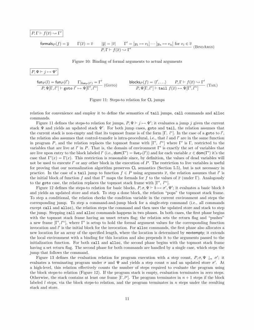
Figure 11 defines the steps-to relation for jumps, P,Ψ ` j 7→ Ψ′; it evaluates a jump j given the currentstack Ψ and yields an updated stack Ψ′. For both jump cases, goto and tail, the relation assumes thatthe current stack is non-empty and that its topmost frame is of the form [Γ, l◦]. In the case of a goto to l′,the relation also assumes that control-transfer is intra-procedural, i.e., that l and l′ are in the same functionin program P , and the relation replaces the topmost frame with [Γ′, l′◦] where Γ′ is Γ, restricted to thevariables that are live at l′ in P . That is, the domain of environment Γ′ is exactly the set of variables thatare live upon entry to the block labeled l′ (i.e., dom(Γ′) = liveP (l′)) and for each variable x ∈ dom(Γ′) it’s thecase that Γ′(x) = Γ(x). This restriction is reasonable since, by definition, the values of dead variables willnot be used to execute l′ or any other block in the execution of P . The restriction to live variables is usefulfor proving that our normalization algorithm preserves CL semantics (Section 5.5), but is not necessary inpractice. In the case of a tail jump to function f ∈ P using arguments x, the relation assumes that l′ isthe initial block of function f and that Γ′ maps the formals for f to the values of x (under Γ). Analogouslyto the goto case, the relation replaces the topmost stack frame with [Γ′, l′◦].
Figure 12 defines the steps-to relation for basic blocks, P, σ,Ψ ` b 7→ σ′,Ψ′; it evaluates a basic block band yields an updated store and stack. To step a done block, the relation “pops” the topmost stack frame.To step a conditional, the relation checks the condition variable in the current environment and steps thecorresponding jump. To step a command-and-jump block for a single-step command (i.e., all commandsexcept call and alloc), the relation steps the command and then uses the updated store and stack to stepthe jump. Stepping call and alloc commands happens in two phases. In both cases, the first phase beginswith the topmost stack frame having an unset return flag; the relation sets the return flag and “pushes”a new frame [Γ′, l′◦], where Γ′ is setup to hold the formal argument values for the corresponding functioninvocation and l′ is the initial block for the invocation. For alloc commands, the first phase also allocates anew location for an array of the specified length, where the location is determined by nextempty; it extendsthe local environment with a binding for this location and also prepends it to the arguments passed to theinitialization function. For both call and alloc, the second phase begins with the topmost stack framehaving a set return flag. The second phase for both commands are handled by a single case, which steps thejump that follows the command.
Figure 13 defines the evaluation relation for program execution with a step count, P, σ,Ψ ↓n σ′; itevaluates a terminating program under σ and Ψ and yields a step count n and an updated store σ′. Ata high-level, this relation effectively counts the number of steps required to evaluate the program usingthe block steps-to relation (Figure 12). If the program stack is empty, evaluation terminates in zero steps.Otherwise, the stack contains at least one frame [Γ, lρ]. The program terminates in n+ 1 steps if the blocklabeled l steps, via the block steps-to relation, and the program terminates in n steps under the resultingstack and store.
11

P, σ,Ψ ` b 7→ σ′,Ψ′
P, σ,Ψ[Γ, l◦] ` {l : done} 7→ σ,Ψ(Done)
(Γ(x) 6= 0 ∧ j = j1) ∨ (Γ(x) = 0 ∧ j = j2) P,Ψ[Γ, l◦] ` j 7→ Ψ′
P, σ,Ψ[Γ, l◦] ` {l : cond x j1 j2} 7→ σ,Ψ′(Cond)
σ,Γ ` c 7→ σ′,Γ′ P,Ψ[Γ′, l◦] ` j 7→ Ψ′
P, σ,Ψ[Γ, l◦] ` {l : c ; j} 7→ σ′,Ψ′(CmdJmp)
blocksP (f) = 〈l′, . . .〉 P,Γ ` f(x) ; Γ′
P, σ,Ψ[Γ, l◦] ` {l : call f(x); j} 7→ σ,Ψ[Γ, l•][Γ′, l′◦](Call)
Γ(y) = n nextempty(σ) = `σ′ = σ[` 7→ array 0n] Γ′ = Γ[x 7→ `] blocksP (f) = 〈l′, . . .〉 P,Γ′ ` f(x :: z) ; Γ′′
P, σ,Ψ[Γ, l◦] ` {l : x := alloc y f z ; j} 7→ σ′,Ψ[Γ′, l•][Γ′′, l′◦](Alloc)
P,Ψ[Γ, l◦] ` j 7→ Ψ′
P, σ,Ψ[Γ, l•] ` {l : c ; j} 7→ σ,Ψ′(RetJmp)
Figure 12: Steps-to relation for CL basic blocks
P, σ,Ψ ↓n σ′
P, σ, · ↓0 σ(Halt)
blockP (l) = b P, σ,Ψ[Γ, lρ] ` b 7→ σ′,Ψ′ P, σ′,Ψ′ ↓n σ′′
P, σ,Ψ[Γ, lρ] ↓n+1 σ′′ (Run)
Figure 13: Program execution with step count
5 Normalizing CL Programs
We say that a program is in normal form if and only if every read command is in a tail-jump block, i.e.,followed immediately by a tail jump. In this section, we describe an algorithm for normalization thatrepresents programs with control flow graphs and uses dominator trees to restructure them. Section 5.4illustrates the techniques described in this section applied to our running example.
5.1 Program Graphs
We represent CL programs with a particular form of rooted control flow graphs, which we shortly refer to asa program graph or simply as a graph when it is clear from the context.
The graph for a program P consists of nodes and edges, where each node represents a function definition,a (basic) block, or a distinguished root node (Section 5.4 shows an example). We tag each non-root nodewith the label of the block or the name of the function that it represents. Additionally, we tag each noderepresenting a block with the code for that block and each node representing a function, called a functionnode, with the prototype (name and arguments) of the function and the declaration of local variables. As amatter of notational convenience, we name the nodes with the label of the corresponding basic block or thename of the function, e.g., ul or uf .
12

The edges of the graph represent control transfers. For each goto jump belonging to a block {k :c ; goto l}, we have an edge from node uk to node ul tagged with goto l. For each function node ufwhose first block is ul, we have an edge from uf to ul labeled with goto l. For each tail-jump block{k : c ; tail f(x)}, we have an edge from uk to uf tagged with tail f(x). If a node uk represents acall-instruction belonging to a block {k : call f(x) ; j}, then we insert an edge from uk to uf and tag itwith call f(x). For each conditional block {k : cond x j1 j2} where j1 and j2 are the jumps, we insertedges from k to targets of j1 and j2, tagged with true and false, respectively.
We call a node a read-entry node if it is the target of an edge whose source is a read node. Morespecifically, consider the nodes uk belonging to a block of the form {k : x := read y ; j} and ul which isthe target of the edge representing the jump j; the node ul is a read entry. We call a node an entry node ifit is a read-entry or a function node. For each entry node ul, we insert an edge from the root to ul into thegraph.
There is a (efficiently) computable isomorphism between a program and its graph that enables us to treatprograms and graphs as a single object. In particular, by changing the graph of a program, our normalizationalgorithm effectively restructures the program itself.
Lemma 1 (Programs and Graphs)The program graph of a CL program with n blocks can be constructed in expected O(n) time. Conversely,given a program graph with m nodes, we can construct its program in O(m) time.
Proof: We construct the graph in two passes over the program. In the first pass, we create a root node andcreate a node for each block. We insert the nodes for the blocks into a hash table that maps the block labelto the node. In the second pass, we insert the edges by using the hash table to locate the source and thetarget nodes. Since hash tables require expected constant time per operation, creating the program graphrequires time in the number of blocks of the graph.
To construct the program for a graph, we follow the outgoing edges of the root. By the definition of theprogram graph, each function node is a target of an edge from the root. For each such node, we create afunction definition. We then generate the code for the function by generating the code for each block thatis reachable from the function node via goto edges. Since blocks and edges are tagged with the instructionsthat they correspond to, it is straightforward to generate the code for each node. Finally, the orderingof the functions and the blocks in the functions can be arbitrary, because all control transfers are explicit.Thus, we can generate the code for a program graph by performing a single pass over the program code. �
5.2 Dominator Trees and Units
Let G = (V,E) be a rooted program graph with root node ur. Let uk, ul ∈ V be two nodes of G. We say thatuk dominates ul if every path from ur to ul in G passes through uk. By definition, every node dominatesitself. We say that uk is an immediate dominator of ul if uk 6= ul and uk is a dominator of ul such that everyother dominator of ul also dominates uk. It is easy to show that each node except for the root has a uniqueimmediate dominator (e.g., [25]). The immediate-dominator relation defines a tree, called a dominator treeT = (V,EI) where by EI = {(uk, ul) | uk is an immediate dominator of ul}.
Let T be a dominator tree of a rooted program graph G = (V,E) with root ur. Note that the root of Gand T are both the same. Let ul be a child of ur in T . We define the unit of ul as the vertex set consistingof ul and all the descendants of ul in T ; we call ul the defining node of the unit. Normalization is madepossible by an interesting property of units and cross-unit edges.
Lemma 2 (Cross-Unit Edges)Let G = (V,E) be a rooted program graph and T be its dominator tree. Let Uk and Um be two distinctunits of T defined by vertices uk and um respectively . Let ul ∈ Uk and un ∈ Um be any two vertices fromUk and Um. If (ul, un) ∈ E, i.e., a cross-unit edge in the graph, then un = um.
13

1 NORMALIZE (P) =
2 Let G = (V,E) be the graph of P rooted at ur
3 Let T be the dominator tree of G (rooted at ur)
4 G′ = (V ′, E′), where V ′ = V and E′ = ∅5 for each unit U of T do
6 ul ← defining node of U7 if ul is a function node then
8 (* ul is not critical *)
9 EU ← {(ul, u) ∈ E | (u ∈ U)}10 else
11 (* ul is critical *)
12 pick a fresh function f, i.e., f 6∈ funs(P )13 let x be the live variables at l in P14 let y be the free variables in U15 z = y \ x16 V ′ ← V ′ ∪ {uf}17 tag(uf ) = f(x){z}18 EU ← {(ur, uf ), (uf , ul)} ∪19 {(u1, u2) ∈ E | u1, u2 ∈ U ∧ u2 6= ul}20 for each critical edge (uk, ul) ∈ E do
21 if uk 6∈ U then
22 (* cross-unit edge *)
23 EU ← EU ∪ {(uk, uf )}24 tag((u, uf )) = tail f(x)25 else
26 (* intra-unit edge *)
27 if uk is a read node then
28 EU ← EU ∪ {(uk, uf )}29 tag((u, uf )) = tail f(x)30 else
31 EU ← EU ∪ {(uk, ul)}32 E′ ← E′ ∪ EU
Figure 14: Pseudo-code for the normalization algorithm.
Proof: Let ur be the root of both T and G. For a contradiction, suppose that (ul, un) ∈ E and un 6= um.Since (ul, un) ∈ E there exists a path p = ur ; uk ; ul → un in G. Since um is a dominator of un, thismeans that um is in p, and since um 6= un it must be the case that either uk proceeds um in p or vice versa.We consider the two cases separately and show that they each lead to a contradiction.
• If uk proceeds um in p then p = ur ; uk ; um ; ul → un. But this means that ul can be reachedfrom ur without going through uk (since ur → um ∈ G). This contradicts the assumption that ukdominates ul.
• If um proceeds uk in p then p = ur ; um ; uk ; ul → un. But this means that un can be reachedfrom ur without going through um (since ur → uk ∈ G). This contradicts the assumption that umdominates un. �
5.3 An Algorithm for Normalization
Figure 14 gives the pseudo-code for our normalization algorithm, NORMALIZE. At a high level, the algorithmrestructures the original program by creating a function from each unit and by changing control transfersinto these units to tail jumps as necessary.
14

Given a program P , we start by computing the graph G of P and the dominator tree T of G. Let urbe the root of the dominator tree and the graph. The algorithm computes the normalized program graphG′ = (V ′, E′) by starting with a vertex set equal to that of the graph V ′ = V and an empty edge set E′ = ∅.It proceeds by considering each unit U of T .
Let U be a unit of T and let the node ul of T be the defining node of the unit. If ul is a not a functionnode, then we call it and all the edges that target it critical. We consider two cases to construct a set ofedges EU that we insert into G′ for U . If ul is not critical, then EU consists of all the edges whose target isin U . If ul is critical, then we define a function for it by giving it a fresh function name f and computingthe set of live variables x at block l in P , and free variables y in all the blocks represented by U . The setx becomes the formal arguments to the function f and the set z of variables defined as the remaining freevariables, i.e., y \ x, become the locals. We then insert a new node uf into the normalized graph and insertthe edges (ur, uf ) and (uf , ul) into EU as well as all the edges internal to U that do not target ul. Thiscreates the new function f(x) with locals z whose body is defined by the basic blocks of the unit U . Next,we consider critical edges of the form (uk, ul). If the edge is a cross-unit edge, i.e., uk 6∈ U , then we replaceit with an edge into uf by inserting (uk, uf ) into EU and tagging the edge with a tail jump to the definedfunction f representing U . If the critical edge is an intra-unit edge, i.e., uk ∈ U , then we have two cases toconsider: If uk is a read node, then we insert (uk, uf ) into EU and tag it with a tail jump to function f withthe appropriate arguments, effectively redirecting the edge to uf . If uk is not a read node, then we insertthe edge into EU , effectively leaving it intact. Although the algorithm only redirects critical edges Lemma 2shows this is sufficient: all other edges in the graph are contained within a single unit and hence do not needto be redirected.
At a high level, the algorithm computes the program graph and the units of the graph. It then processeseach unit so that it can assign a function to each unit. If a unit’s defining vertex is a function node, thenno changes are required and all non-dominator-tree edges incident on the vertices of the unit are inserted.If the units defining vertex is not a function node, then the algorithm creates a function for that unit byinserting a function node uf between the defining node and the node. It then makes a function for eachunit and replaces cross unit edges with tail-jump edge to this function. Since all cross unit have the definingnode of a unit as their target, this replaces all cross-unit control transfers with tail jumps, ensuring that allcontrol branches (except for function calls, tail or not) remain local. The algorithm preserves the intra-unitedges that do not target the defining node. The algorithm replaces each intra-unit edge, whose target is thedefining node of the unit, with a tail-jump edge to the new function node if the source of that edge is a readnode. This ensures that read instructions transfer control to the defining node of a unit with a tail jump tothe function node for that unit.
5.4 Example
Figure 15 shows the rooted graph for the expression-tree evaluator shown in Figure 2 after translating itinto CL (Section 4.3). The nodes are labeled with the line numbers that they correspond to; goto edgesand control-branches are represented as straight edges, and (tail) calls are represented with curved edges.For example, node 0 is the root of the graph; node 1 is the entry node for the function eval; node 3 is theconditional on line 3; the nodes 8 and 9 are the recursive calls to eval. The nodes 3, 11, 12 are read-entrynodes. Figure 16 shows the dominator tree for the graph (Figure 15). For illustrative purposes the edges ofthe graph that are not tree edges are shown as dotted edges.5 The units are defined by the vertices 1, 3, 11,12, 18. The cross-unit edges, which are non-tree edges, are (2,3), (4,18), (10,11), (11,12), (13,18), (15,18).Note that as implied by Lemma 2, all these edges target the defining nodes of the units.
Figure 17 shows the rooted program graph for the normalized program created by algorithm NORMALIZE.By inspection of Figures 16 and 2, we see that the critical nodes are 3, 11, 12, 18, because they defineunits but they are not function nodes. The algorithm creates the fresh nodes a, b, c, and d for these unitsand redirects all the cross-unit edges into the new function nodes and tagged with tail jumps (tags notshown). In this example, we have no intra-unit critical edges. Figure 5 shows the code for the normalizedgraph (described in Section 3.2).
5Note that the dominator tree can have edges that are not in the graph.
15

2
1
64
3
7
15
8
10
9
12
11
13
0
18
Figure 15: Theprogram graphof eval.
2
1
64
3
7
15
8
11
9
12
13
0
18
10
treenontree
Figure 16: The dominator treefor the graph in Figure 15.
2
1
64
3
7
15
8
11
9
12
13
0
18
10
b c da
Figure 17: Normalized version of thegraph in Figure 15.
5.5 Properties of Normalization
We state and prove some properties about the normalization algorithm and the (normal) programs it pro-duces. The normalization algorithm uses a live variable analysis to determine the formal and actual argu-ments for each fresh function (see line 13 in Figure 14). We let TL(P ) denote the time required for livevariable analysis of a CL program P . The output of this analysis for program P is a function live(·), wherelive(l) is the set variables which are live at (the start of) block l ∈ P . We let ML(P ) denote the maximumnumber of live variables for any block in program P , i.e., maxl∈P |live(l)|. We assume that each variable,function name, and block label require one word to represent. The following theorems relate the size of a CLprogram before and after normalization (Theorem 3) and bound the time required to perform normalization(Theorem 4).
Theorem 3 (Size of Output Program)If CL program P has n blocks and P ′ = NORMALIZE(P ), then P ′ also has n blocks and at most n additionalfunction definitions. Furthermore if it takes m words to represent P , then it takes O(m+ n ·ML(P )) wordsto represent P ′.
Proof: Observe that the normalization algorithm creates no new blocks—just new function nodes. Fur-thermore, since at most one function is created for each critical node, which is a block, the algorithm createsat most one new function for each block of P . Thus, the first bound follows.
For the second bound, note that since we create at most one new function for each block, we can nameeach function using the block label followed by a marker (stored in a word), thus requiring no more than2n words. Since each fresh function has at most ML(P ) arguments, representing each function signaturerequires O(ML(P )) additional words (note that we create no new variable names). Similarly, each call toa new function requires O(ML(P )) words to represent. Since the number of new functions and new calls isbounded by n, the total number of additional words needed for the new function signatures and the newfunction calls is bounded by O(m+ n ·ML(P )). �
16

Theorem 4 (Time for Normalization)If CL program P has n blocks then running NORMALIZE(P ) takes O(n+ n ·ML(P ) + TL(P )) time.
Proof: Computing the dominator tree takes linear time [19]. By definition, computing the set of live vari-ables for each node takes TL(P ) time. We show that the remaining work can be done in O(n+ n ·ML(P ))time. To process each unit, we check if its defining node is a function node. If so, we copy each incomingedge from the original program. If not, we create a fresh function node, copy non-critical edges, and processeach incoming critical edge. Since each node has a constant out degree (at most two), the total number ofedges considered per node is constant. Since each defining node has at most ML(P ) live variables, it takesO(ML(P )) time to create a fresh function. Replacing a critical edge with a tail jump edge requires creatinga function call with at most ML(P ) arguments, requiring O(ML(P )) time. Thus, it takes O(n+ n ·ML(P ))time to process all the units. �
We use the formal semantics described in Section 4.4 to state and prove that our algorithm for normal-ization preserves the extensional (input-output behavior) and the intensional (time and space requirement)semantics of CL programs. First, we prove that normalization preserves the basic block step relation (Fig-ure 12), and then use this result to prove that it preserves CL program execution as defined by the programexecution relation (Figure 13). In particular, the heap & stack usage and the step count (i.e., executiontime) are each preserved by our algorithm.
Lemma 5 (Normalization preserves block steps)If P ′ = NORMALIZE(P ) and P, σ1,Ψ1 ` b 7→ σ2,Ψ2 and b ∈ P corresponds to b′ ∈ P ′ (i.e., b and b′ have thesame label l) then P ′, σ1,Ψ1 ` b′ 7→ σ2,Ψ2.
Proof: By inspection, the NORMALIZE algorithm does not add or remove basic blocks, nor does it changetheir labels or tags in the program graph (e.g., it preserves the commands of command-and-jump blocksand the conditions of conditional blocks). In fact, it only changes the jumps in basic blocks by replacingparticular jump edges. Therefore, since b and b′ have the same label, they also have the same tag in theirrespective program graphs. That is, we can conclude the following:
• If b is a done block, then b′ is also a done block.
• If b is a condition block {l : cond x j1 j2}, then b′ is a condition block of the form {l : cond x j′1 j′2}.
• If b is a command-and-jump block {l : c ; j} then b′ is a command-and-jump block of the form {l : c ; j′}.
In each case, the blocks b and b′ only differ in the jumps they contain (and in the case of done blocks, theynever differ). Hence, it suffices to show that for each jump j in the block b and corresponding jump j′ in theblock b′ the following implication holds:
P,Ψ1 ` j 7→ Ψ2 =⇒ P ′,Ψ1 ` j′ 7→ Ψ3 and Ψ2 = Ψ3
If j = j′ then the implication holds trivially. If j 6= j′ then by inspection of the NORMALIZE algorithm weknow that j corresponds to a critical edge in P . Furthermore, we see that j = goto l′, for some blockl′, and j′ = tail f(x) where f is a new function with initial block l′ and x are the live variables at l′
in the original program. To show the implication holds in this case, assume that the antecedent holds,which means Ψ1 = Ψ[Γ, l◦] for some Ψ, Γ and l. Since we know j = goto l′, by the jump step relationwe have that Ψ2 = [Γ′, l′◦], where Γ′ is Γ, restricted to the live variables at l. Now consider Ψ3. We knowthat j′ = tail f(x) and that l′ is the initial block of f , and we also know that x are the live variablesat l′ in P (i.e., the domain of Γ′). Therefore P ′,Γ ` f(x) ; Γ′ and hence, by the jump step relation,Ψ3 = Ψ[Γ′, l′◦] = Ψ2. This completes the proof. �
17

Theorem 6 (Normalization preserves semantics)If P ′ = NORMALIZE(P ) and P, σ,Ψ ↓n σ′ then P ′, σ,Ψ ↓n σ′.
Proof: By induction of the derivation of P, σ,Ψ ↓n σ′ using the step-counting relation (Figure 13). Thereare two cases to consider, which respectively correspond to the two cases for the final derivation step.
1. Consider the case for n = 0, and assume the antecedent holds to show that the consequent holds. Sincethe antecedent holds and n = 0, by inspection of the step counting relation we have that Ψ = ·, andthat σ = σ′. Since P ′, σ, · ↓0 σ for any P ′ and σ, we get the desired result.
2. Consider the case for n + 1. Assume that the antecedent holds and that the theorem holds for n toshow that the consequent holds for n+1. Since the antecedent holds, by inspection of the step countingrelation we have that:
(a) P, σ,Ψ ↓n+1 σ′
(b) Ψ = Ψ1[Γ, lρ], for some Ψ1
(c) blockP (l) = b, for some block b ∈ P(d) P, σ,Ψ ` b 7→ σ2,Ψ2, for some σ2 and Ψ2
(e) P, σ2,Ψ2 ↓n σ′
It remains to show the derivation step for P ′, σ,Ψ ↓n+1 σ′. Recall that NORMALIZE preserves each label
of the original program so that if l is a label in P then l is also a label for some block in P ′. Assumethat blockP ′(l) = b′ for some block b′ ∈ P ′. By applying Lemma 5 to (2d) with respect to b in P andb′ in P ′, we have that
P ′, σ,Ψ ` b′ 7→ σ2,Ψ2
Since the theorem holds for n, we can apply it to (2e) and have that
P ′, σ2,Ψ2 ↓n σ′
By application of the step counting relation with these results, we get the desired consequent:
P ′, σ,Ψ ↓n+1 σ′
This completes the cases and the proof. �
Corollary 7 (Normalization preserves time and space)As direct corollaries to Theorem 6, NORMALIZE preserves the following:
• Time to execute the program (in block steps)
• Stack space used by the program
• Heap space used by the program
Stack Space In Practice Formally, we model the stack with Ψ, which is in turn defined by a series ofstack frames, each containing an environment Γ. As in the formal semantics, in practice we push a newstack frame to perform a function call, replace the current stack frame to perform a tail jump, and popthe current stack frame when a function completes. Unlike in the formalism, however, in practice thesestack frames are implemented as mutable objects in memory that are side-effected, rather than replaced,to perform assignments to local variables. Moreover, in practice we do not contract the stack frame to livevariables when performing goto jumps since this is practically unnecessary. However, note that normalizedprograms essentially perform this contraction for each goto jump that becomes a tail jump, since such tailjumps pass only the values of live variables, and thus, may replace the topmost stack frame with a smallerone (and never a larger one). Therefore, in practice, although a normalized program will use the samestack space when measured by the number of frames (for this metric, Theorem 6 still applies), a normalizedprogram may use less stack space the original program when measured by the number of values (or bytes).
18

typedef struct {. . .} closure t;
closure t* closure make(closure t* (*f)(τ x), τ x);void closure run(closure t* c);
typedef struct {. . .} modref t;
void modref init(modref t *m);
void modref write(modref t *m, void *v);closure t* modref read(modref t *m, closure t *c);
void* allocate(size t n, closure t *c);
Figure 18: The interface for the run-time system.
6 Translation to C
The translation phase translates normalized CL code into C code that relies on a run-time system providingself-adjusting computation primitives. To support tail jumps in C without growing the stack we adapt awell-known technique called trampolining (e.g., [23, 35]). At a high level, a trampoline is a loop that runs asequence of closures that, when executed, either return another closure or NULL, which signals the trampolineto terminate.
6.1 The Run-Time System
Figure 18 shows the interface to the run-time system (RTS). The RTS provides functions for creating andrunning closures. The closure make function creates a closure given a function and a complete set ofmatching arguments. The closure run function sets up a trampoline for running the given closure (and theclosures it returns, if any) iteratively. The RTS provides functions for creating, reading, and writing modi-fiables (modref t). The modref init function initializes memory for a modifiable; together with allocatethis function can be used to allocate modifiables. The modref write function updates the contents of amodifiable with the given value. The modref read function reads a modifiable, substitutes its contents asthe first argument of the given closure, and returns the updated closure. The allocate function allocates amemory block with the specified size (in bytes), runs the given closure after substituting the address of theblock for the first argument, and returns the address of the block. The closure acts as the initializer for theallocated memory.
6.2 The Basic Translation
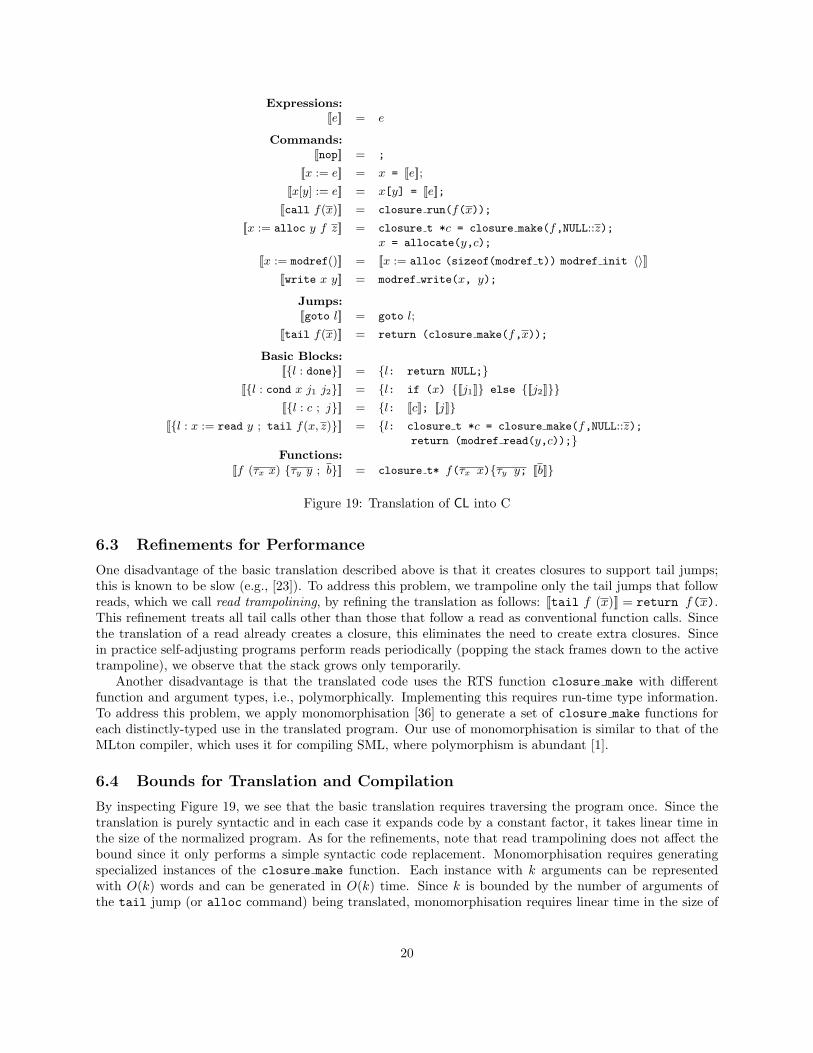
Figure 19 illustrates the rules for translating normalized CL programs into C. For clarity, we deviate from Csyntax slightly by using := to denote the C assignment operator.
The most interesting cases concern function calls, tail jumps, and modifiables. To support trampolining,we translate functions to return closures. A function call is translated into a direct call whose return value(a closure) is passed to a trampoline, closure run. A tail jump simply creates a corresponding closure andreturns it to the active trampoline. Since each tail jump takes place in the context of a function, there isalways an active trampoline. The translation of alloc first creates a closure from the given initializationfunction and arguments prepended with NULL, which acts as a place-holder for the allocated location. Itthen supplies this closure and the specified size to allocate.
We translate modref as a special case of allocation by supplying the size of a modifiable and usingmodref init as the initialization function. Translation of write commands is straightforward. We translatea command-and-jump block by separately translating the command and the jump. We translate reads tocreate a closure for the tail jump following the read command and call modref read with the closure & themodifiable being read. As with tail jumps, the translated code returns the resulting closure to the activetrampoline. When creating the closure, we assume, without loss of generality, that the result of the readappears as the first argument to the tail jump and use NULL as a placeholder for the value read. Note that,since translation follows normalization, all read commands are followed by a tail jump, as we assume here.
19
Expressions:[[e]] = e
Commands:[[nop]] = ;
[[x := e]] = x = [[e]];
[[x[y] := e]] = x[y] = [[e]];
[[call f(x)]] = closure run(f(x));
[[x := alloc y f z]] = closure t *c = closure make(f,NULL::z);x = allocate(y,c);
[[x := modref()]] = [[x := alloc (sizeof(modref t)) modref init 〈〉]][[write x y]] = modref write(x, y);
Jumps:[[goto l]] = goto l;
[[tail f(x)]] = return (closure make(f,x));
Basic Blocks:[[{l : done}]] = {l: return NULL;}
[[{l : cond x j1 j2}]] = {l: if (x) {[[j1]]} else {[[j2]]}}[[{l : c ; j}]] = {l: [[c]]; [[j]]}
[[{l : x := read y ; tail f(x, z)}]] = {l: closure t *c = closure make(f,NULL::z);return (modref read(y,c));}
Functions:
[[f (τx x) {τy y ; b}]] = closure t* f(τx x){τy y; [[b]]}
Figure 19: Translation of CL into C
6.3 Refinements for Performance
One disadvantage of the basic translation described above is that it creates closures to support tail jumps;this is known to be slow (e.g., [23]). To address this problem, we trampoline only the tail jumps that followreads, which we call read trampolining, by refining the translation as follows: [[tail f (x)]] = return f(x).This refinement treats all tail calls other than those that follow a read as conventional function calls. Sincethe translation of a read already creates a closure, this eliminates the need to create extra closures. Sincein practice self-adjusting programs perform reads periodically (popping the stack frames down to the activetrampoline), we observe that the stack grows only temporarily.
Another disadvantage is that the translated code uses the RTS function closure make with differentfunction and argument types, i.e., polymorphically. Implementing this requires run-time type information.To address this problem, we apply monomorphisation [36] to generate a set of closure make functions foreach distinctly-typed use in the translated program. Our use of monomorphisation is similar to that of theMLton compiler, which uses it for compiling SML, where polymorphism is abundant [1].
6.4 Bounds for Translation and Compilation
By inspecting Figure 19, we see that the basic translation requires traversing the program once. Since thetranslation is purely syntactic and in each case it expands code by a constant factor, it takes linear time inthe size of the normalized program. As for the refinements, note that read trampolining does not affect thebound since it only performs a simple syntactic code replacement. Monomorphisation requires generatingspecialized instances of the closure make function. Each instance with k arguments can be representedwith O(k) words and can be generated in O(k) time. Since k is bounded by the number of arguments ofthe tail jump (or alloc command) being translated, monomorphisation requires linear time in the size of
20

the normalized code. Thus, we conclude that we can translate a normalized program in linear time whilegenerating C code whose size is within a constant factor of the normalized program. Putting together thisbound and the bounds from normalization (Theorems 3 and 4), we can bound the time for compilation andthe size of the compiled programs.
Theorem 8 (Compilation)Let P be a CL program with n blocks that requires m words to represent. Let ML(P ) be the maximumnumber of live variables over all blocks of P and let TL(P ) be the time for live-variable analysis. It takesO(n+n·ML(P )+TL(P )) time to compile the program into C. The generated C code requires O(m+n·ML(P ))words to represent.
7 Implementation
The implementation of our compiler, cealc, consists of a front-end and a runtime library. The front-endtransforms CEAL code into C code. We use an off-the-shelf compiler (gcc) to compile the translated codeand link it with the runtime library.
Our front-end uses an intra-procedural variant of our normalization algorithm that processes each corefunction independently from the rest of the program, rather than processing the core program as a whole(as presented in Section 5). This works because inter-procedural edges (i.e., tail jump and call edges) in arooted graph don’t impact its dominator tree—the immediate dominator of each function node is always theroot. Hence, the subgraph for each function can be independently analyzed and transformed. Since eachfunction’s subgraph is often small compared to the total program size, we use a simple, iterative algorithmfor computing dominators [29, 14] that is efficient on smaller graphs, rather than an asymptotically optimalalgorithm with larger constant factors [19]. During normalization, we create new functions by computingtheir formal arguments as the live variables that flow into their entry nodes in the original program graph.We use a standard, intra-procedural liveness analysis for this step (e.g., [29, 7]).
Our front-end is implemented as an extension to CIL (C Intermediate Language), a library of tools usedto parse, analyze and transform C code [30]. We provide the CEAL core and mutator primitives as ordinaryC function prototypes. We implement the ceal keyword as a typedef for void. Since these syntacticextensions are each embedded within the syntax of C, we define them with a conventional C header fileand do not modify CIL’s C parser. To perform normalization, we identify the core functions (which aremarked by the ceal return type) and apply the intra-procedural variant of the normalization algorithm.The translation from CL to C directly follows the discussions in Section 6. We translate mutator primitivesusing simple (local) code substitution.
Our runtime library provides an implementation of the interface discussed in Section 6. The implemen-tation is built on previous work which focused on efficiently supporting automatic memory management forself-adjusting programs. We extend the previous implementation with support for tail jumps via trampolin-ing, and support for imperative (multiple-write) modifiable references [4].
Our front-end extends CIL with about 5,000 lines of additional Objective Caml (OCaml) code, andour runtime library consists of about 5,000 lines of C code. Our implementation is available online athttp://ttic.uchicago.edu/~ceal.
8 Experimental Results
We present an empirical evaluation of our implementation.
8.1 Experimental Setup and Measurements
We run our experiments on a 2Ghz Intel Xeon machine with 32 gigabytes of memory running Linux (kernelversion 2.6). All our programs are sequential (no parallelism). We use gcc version 4.2.3 with “-O3” to
21

compile the translated C code. All reported times are wall-clock times measured in milliseconds or seconds,averaged over five independent runs.
For each benchmark, we consider a self-adjusting and a conventional version. Both versions are derivedfrom a single CEAL program. We generate the conventional version by replacing modifiable references withconventional references, represented as a word-sized location in memory that can be read and written.Unlike modifiable references, the operations on conventional references are not traced and thus conventionalprograms are not normalized. The resulting conventional versions are essentially the same as the static Ccode that a programmer would write for that benchmark.
For each self-adjusting benchmark we measure the time required for propagating a small modificationby using a special test mutator. Invoked after an initial run of the self-adjusting version, the test mutatorperforms two modifications for each element of the input: it deletes the element and performs changepropagation, it inserts the element back and performs change propagation. We report the average time fora modification as the total running time of the test mutator divided by the number of updates performed(usually two times the input size).
For each benchmark we measure the from-scratch running time of the conventional and the self-adjustingversions; we define the overhead as the ratio of the latter to the former. The overhead measures the slowdowncaused by the dependence tracking techniques employed by self-adjusting computation. We measure thespeedup for a benchmark as the ratio of the from-scratch running time of the conventional version dividedby the average modification time computed by running the test mutator.
8.2 Benchmark Suite
Our benchmarks include list primitives, and more sophisticated algorithms for computational geometry andtree computations.
List Primitives. Our list benchmarks include the list primitives filter, map, and reverse, minimum, andsum, which we expect to be self-explanatory, and the sorting algorithms quicksort and mergesort. Ourmap benchmark maps each number x of the input list to f(x) = bx/3c + bx/7c + bx/9c in the output list.Our filter benchmark filters out an input element x if and only if f(x) is odd. Our reverse benchmarkreverses the input list. The list reductions minimum and sum find the minimum and the maximum elementsin the given lists. We generate lists of n (uniformly) random integers as input for the list primitives. Forsorting algorithms, we generate lists of n (uniformly) random, 32-character strings.
Computational Geometry. Our computational-geometry benchmarks are quickhull, diameter, anddistance; quickhull computes the convex-hull of a point set using the classic algorithm with the samename; diameter computes the diameter (the maximum distance between any two points) of a point set;distance computes the minimum distance between two sets of points. The implementations of diameterand distance use quickhull as a subroutine. For quickhull and distance, input points are drawn from auniform distribution over the unit square in R2. For distance, two non-overlapping unit squares in R2 areused, and from each square we draw half the input points.
Tree-based Computations. The exptrees benchmark is a variation of our simple running example,and it uses floating-point numbers in place of integers. We generate random, balanced expression trees asinput and perform modifications by changing their leaves. The tcon benchmark is an implementation of thetree-contraction technique by Miller and Reif [27]. This this a technique rather than a single benchmarkbecause it can be customized to compute various properties of trees, e.g., [27, 28, 6]. For our experiments,we generate binary input trees randomly and perform a generalized contraction with no application-specificdata or information. We measure the average time for an insertion/deletion of edge by iterating over all theedges as with other applications.
22

0.010.020.030.040.050.060.070.080.090.0
4M3M2M1M0
Tim
e (s
)
Input Size
CEAL (from-scratch)C (from-scratch).
0
0.05
0.1
0.15
0.2
4M3M2M1M0
Tim
e (m
s)
Input Size
CEAL (propagate)
0.0 x 1001.0 x 1042.0 x 1043.0 x 1044.0 x 1045.0 x 1046.0 x 1047.0 x 1048.0 x 1049.0 x 1041.0 x 105
4M3M2M1M0
Input Size
CEAL (Speedup)
Figure 20: Experimental results for tcon (self-adjusting tree-contraction).
0
20
40
60
80
100
0 1M 2M 3M 4M
Tim
e (s
)
Input Size
CEAL (from-scratch)RC-Trees (from-scratch)C (from-scratch)
0
0.05
0.1
0.15
0.2
0 1M 2M 3M 4M
Tim
e (m
s)Input Size
CEAL (propagate)RC-Trees (update)
Figure 21: Comparison between CEAL and RC-Trees [6] performing (self-adjusting) tree contraction.
8.3 Results
For brevity, we illustrate detailed results for one of our benchmarks, tree contraction (tcon), and summarizethe others. Figure 20 shows the results with tcon. The leftmost figure compares times for a from-scratch runof the conventional and self-adjusting versions; the middle graph shows the time for an average update; andthe rightmost graph shows the speedup. The results show that self-adjusting version is slower by a constantfactor (of about 8) than the conventional version. Change propagation time increases slowly (logarithmically)with the input size. This linear-time gap between recomputing from scratch and change propagation yieldsspeedups that exceed four orders of magnitude even for moderately sized inputs.
Figure 21 compares our implementation to that of an hand-optimized implementation written in C++(labeled “RC-Trees”) [6]. The comparison shows that RC-Trees is only 3–4 times faster than the CEALimplementation. We interpret this is as a very encouraging result for the effectiveness of our compiler, whichdoes not perform significant optimizations.
Table 1 summarizes our results for CEAL benchmarks at fixed input sizes of 1 million (written “1.0M”)and 10 million (written “10.0M”). From left to right, for each benchmark, we report the input size considered,the time for conventional and self-adjusting runs, the overhead, the average time for an update, the speedup,and the maximum live memory required for running the experiments (both from-scratch and test mutatorruns). The individual graphs for these benchmarks resemble that of the tree contraction (Figure 20). Forthe benchmarks run with input size 10M, the average overhead is 14.2 and the average speedup is 1.4× 10⁵;for those run with input size 1M, the average overhead is 9.2 and the average speedup is 3.6× 10⁴. We notethat for all benchmarks the speedups are scalable and continue to increase with larger input sizes.
8.4 Full Trampolining
To measure the effectiveness of read trampolining, where closures are created, traced and trampolined onlyfor tail jumps that follow reads, we compare results for two of our benchmarks, sum and minimum, to the
23

From-Scratch PropagationApplication n Cnv. Self. O.H. Ave. Update Speedup Max Livefilter 10.0M 0.5 7.4 14.2 2.1× 10⁻⁶ 2.4× 10⁵ 3017.2Mmap 10.0M 0.7 11.9 17.2 1.6× 10⁻⁶ 4.2× 10⁵ 3494.6M
reverse 10.0M 0.6 11.9 18.8 1.6× 10⁻⁶ 3.9× 10⁵ 3494.6Mminimum 10.0M 0.8 10.9 13.8 4.8× 10⁻⁶ 1.6× 10⁵ 3819.4Msum 10.0M 0.8 10.9 13.9 7.0× 10⁻⁵ 1.1× 10⁴ 3819.8M
quicksort 1.0M 3.5 22.4 6.4 2.4× 10⁻⁴ 1.4× 10⁴ 8956.7Mquickhull 1.0M 1.1 12.3 11.5 2.3× 10⁻⁴ 4.6× 10³ 6622.9Mdiameter 1.0M 1.0 12.1 12.0 1.2× 10⁻⁴ 8.3× 10³ 6426.9Mexptrees 10.0M 1.0 7.2 7.2 1.4× 10⁻⁶ 7.1× 10⁵ 4821.1Mmergesort 1.0M 6.1 37.6 6.1 1.2× 10⁻⁴ 5.1× 10⁴ 15876.3Mdistance 1.0M 1.0 11.0 11.0 1.3× 10⁻³ 7.5× 10² 5043.6M
rctree-opt 1.0M 2.6 20.6 7.9 1.0× 10⁻⁴ 2.5× 10⁴ 5843.7M
Table 1: Summary of measurements with CEAL; all times in seconds and space in bytes.
result of using “full trampolining”. In full trampolining, we create, trace6 and trampoline closures for everytail jump. By contrast, in read trampolining, we only create closures for the tail jumps that follow reads(See Section 6.3).
From-Scratch PropagationApplication n Cnv. Self. O.H. Ave. Update Speedup Max Liveminimum 10.0M 0.8 24.7 31.1 8.3× 10⁻⁶ 9.6× 10⁴ 6840.1Msum 10.0M 0.8 24.3 31.0 1.3× 10⁻⁴ 6.0× 10³ 6840.1M
Table 2: Measurements with CEAL using full trampolining (for minimum & sum)
Table 2 shows the results of using full trampolining in place of the more selective read trampolining tech-nique. Because these benchmarks tend to have more non-read tail jumps than the others, the additional costsof performing full trampolining for them is quite high. As the table shows, the overheads for the benchmarksare more than double of those in Table 1. Moreover, the speedups delivered by change propagation are eachreduced by 50–60%. The performance contrast between the two trampolining techniques shows that readtrampolining can be a very effective translation refinement for some benchmarks.
8.5 Comparison to SaSML
To measure the effectiveness of the CEAL approach to previously proposed approaches, we compare our im-plementation to SaSML, the state-of-art implementation of self-adjusting computation in SML [26]. Tables 3and 4 show, respectively, the time and space required for the common benchmarks. The measurementswere taken on the same computer as the CEAL measurements, with inputs generated in the same way. Forboth CEAL and SaSML we report the from-scratch run time, the average update time and the maximumlive memory required for the experiment. A column labeled SaSML
CEAL follows each pair of CEAL and SaSMLmeasurements and it reports the ratio of the latter to the former. Since the SaSML benchmarks do not scalewell to the input sizes considered in Table 1, we make this comparison at smaller input sizes—1 million and100 thousand (written “100.0K”).
6In future versions of the RTS, we believe it may be useful to distinguish closures that perform reads from those that do notsince the former must be traced, i.e., recorded in the dynamic dependence graph, whereas the latter only need to be traced ifthe programmer wishes for these closures to be used latter for memoization. In the current RTS, every trampolined closure istraced.
24

From-Scratch (Self.) Propagation Time
Application n CEAL SaSML SaSMLCEAL
CEAL SaSML SaSMLCEAL
filter 1.0M 0.7 6.9 9.3 1.4× 10⁻⁶ 8.7× 10⁻⁶ 6.2map 1.0M 0.8 7.8 9.3 1.6× 10⁻⁶ 1.1× 10⁻⁵ 7.1
reverse 1.0M 0.8 6.7 8.0 1.6× 10⁻⁶ 9.2× 10⁻⁶ 5.8minimum 1.0M 1.1 5.1 4.6 3.4× 10⁻⁶ 3.0× 10⁻⁵ 8.8sum 1.0M 1.1 5.1 4.6 4.8× 10⁻⁵ 1.7× 10⁻⁴ 3.5
quicksort 100.0K 1.6 43.8 26.9 1.6× 10⁻⁴ 2.6× 10⁻³ 15.6quickhull 100.0K 1.0 5.1 5.1 1.0× 10⁻⁴ 3.3× 10⁻⁴ 3.3diameter 100.0K 0.9 5.2 5.8 8.6× 10⁻⁵ 3.7× 10⁻⁴ 4.3
Table 3: Times for CEAL versus SaSML for a common set of benchmarks.
Propagation Max Live
Application n CEAL SaSML SaSMLCEAL
filter 1.0M 306.5M 1333.5M 4.4map 1.0M 344.7M 1519.1M 4.4
reverse 1.0M 344.7M 1446.7M 4.2minimum 1.0M 388.4M 1113.8M 2.9sum 1.0M 388.5M 1132.4M 2.9
quicksort 100.0K 775.4M 3719.9M 4.8quickhull 100.0K 657.9M 737.7M 1.1diameter 100.0K 609.0M 899.5M 1.5
Table 4: Space for CEAL versus SaSML for a common set of benchmarks.
Comparing the CEAL and SaSML figures shows that CEAL is about 5–27 times faster for from-scratchruns (about 9 times faster on average) and 3–16 times faster for change propagation (about 7 times fasteron average). In addition, CEAL consumes up to 5 times less space (about 3 times less space on average).
An important problem with the SaSML implementation is that it relies on traditional tracing garbagecollectors (i.e., the collectors used by most SML runtime systems, including the runtime used by SaSML)which previous work has shown to be inherently incompatible with self-adjusting computation, preventing itfrom scaling to larger inputs [21]. Indeed, we observe that, while our implementation scales to larger inputs,SaSML benchmarks don’t. To illustrate this, we limit the heap size and measure the change-propagationslowdown computed as the time for a small modification (measured by the test mutator) with SaSML dividedby that with CEAL for the quicksort benchmark (Figure 22). Each line ends roughly when the heap sizeis insufficient to hold the live memory required for that input size. As the figure shows, the slowdown is notconstant and increases super linearly with the input size to quickly exceed an order of magnitude (can be ashigh as 75).
8.6 Performance of the Compiler
We evaluate the performance of our compiler, cealc, using test programs from our benchmark suite. Eachof the programs we consider consists of a core, which includes all the core-CEAL code needed to run thebenchmark, and a corresponding test mutator for testing this core. We also consider a test driver programwhich consists of all the test mutators (one for each benchmark) and their corresponding core components.
We compile each program with cealc and record both the compilation time and the size of the outputbinary. For comparison purposes, we also compile each program directly with gcc (i.e., without cealc) bytreating CEAL primitives as ordinary functions with external definitions. Table 8.6 shows the results of the
25

15
30
45
60
75
1K 50K 100K 150K 200K
Slo
wdo
wn
Input Size
2G4G8G
Figure 22: SaSML slowdown compared to CEAL for quicksort
cealc gccProgram Lines Time Size Time SizeExpression trees 422 0.84 74K 0.34 58KList primitives 553 1.87 109K 0.49 61KMergesort 621 2.25 123K 0.54 62KQuicksort 622 2.22 123K 0.54 62KQuickhull 988 3.81 176K 0.72 66KTree contraction 1918 8.16 338K 1.03 76KTest Driver 4229 13.69 493K 2.61 110K
Table 5: Compilation times (in seconds) and binary sizes (in bytes)for some CEAL programs. All compiled with -O0.
comparison. As can be seen, cealc is 3–8 times slower than gcc and creates binaries that are 2–5 timeslarger.
In practice, we observe that the size of core functions can be bounded by a moderate constant. Thus themaximum number of live variables, which is an intra-procedural property, is also bounded by a constant.Based on Theorem 8, we therefore expect the compiled binaries to be no more than a constant factor largerthan the source programs. Our experiments show that this constant to be between 2 and 5 for the consideredprograms.
Theorem 8 implies that the compilation time can bounded by the size of the program plus the time forlive-variable analysis. Since our implementation performs live variables analysis and constructs dominatortrees on a per-function basis (Section 7), and since the sizes of core functions are typically bounded by amoderate constant, these require linear time in the size of the program. We therefore expect to see thecompilation times to be linear in the size of the generated code. Indeed Figure 23 shows that the cealccompilation times increase nearly linearly with size of the compiled binaries.
9 Related Work
We discuss the most closely related work in the rest of the paper. In this section, we mention some otherwork that is related more peripherally.
Incremental and Self-Adjusting Computation. The problem of developing techniques to enable com-putations respond to incremental changes to their output have been studied since the early 80’s. We referthe reader to the survey by Ramalingam and Reps [33] and a recent paper [26] for a more detailed setof references. Effective early approaches to incremental computation either use dependence graphs [16] or
26

0
2
4
6
8
10
12
14
0 100 200 300 400 500T
ime
for
ceal
c (s
ec)
Output size (kilobytes)
cealc time
Figure 23: Time for cealc versus size of binary output.
memoization (e.g., [32, 2]). Self-adjusting computation generalizes dependence graphs techniques by intro-ducing dynamic dependence graphs, which enables a change propagation algorithm update the structure ofthe computation based on data modifications, and combining them with a form of computation memoizationthat permits imperative updates to memory [3].
Dominators. The dominator relation has common use in compilers that perform program analysis andoptimization (e.g., [7, 15, 18]). There are a number of asymptotically efficient algorithms for computing dom-inators (e.g., [25, 19]). In practice simple but asymptotically inefficient algorithms also perform reasonablywell [14]. Our implementation uses the simple algorithm described in many compiler books, e.g., [29].
Tail Calls. We use a selective trampolining to support tail calls efficiently (Section 6). Several otherproposals to supporting tail calls in C exists (e.g., [35, 22, 9, 20]). Peyton Jones summarizes some of thesetechniques [23] and discusses the tradeoffs. The primary advantage of trampolining is that it is fully portable;the disadvantage is its cost, which our compiler reduces by piggy-backing closure creation with those of thereads.
10 Discussions
We discuss some limitations of our approach and propose future research directions.
Syntax and Types for Modifiables. The modifiable primitives read and write assume that the typeof a modifiable’s contents is void*. As a result, their uses sometimes require explicit type coercions (e.g., asin Figure 2). Furthermore, the primitives have a function-like syntax, rather than the familiar C-like syntaxfor dereferencing (reading) and assignment (writing).
It may be possible to support more conventional C syntax and avoid type coercions by generalizing thenotion of a modifiable reference to that of a “modifiable field”. In this approach, the programmer wouldannotate the fields of structs that are subject to change across core updates with a new keyword (e.g., mod)that indicates that the field is modifiable. Accessing (reading) and assigning to (writing) these fields woulduse the same syntax as conventional C structs, which would make the use of modifiable primitives implicit.Just as conventional fields carry type information, each modifiable field would also carry a type that couldbe used to ensure that its uses are well-typed. This approach would generalize modifiable references sincethey could be easily encoded as struct with a single modifiable field.
27

Automatic Minimization of Read Bodies. Conceptually, each read operation in CEAL has an implicit“read body” which consists of the code that uses the read value. Our normalization algorithm approximateseach read body conservatively by assuming that it extends to the end of the function containing the associatedread operation. In general, however, a read value may be used in only a small portion of the body foundby normalization. In these cases it’s often advantageous (though not always necessary) to refactor the coreprogram so that each read body identified by normalization is minimal, i.e., it contains no code that isindependent from the read value. In the proposed approach the programmer can perform this refactoringby hand, but we expect that a compiler mechanism could handle some cases for refactoring automaticallyby employing further data- and control-flow analysis.
Support for Return Values. Currently, core functions in CEAL cannot return values as functions canin C, but instead use destination-passing style (DPS) to communicate results through modifiables. In DPS,the caller provides one or more destinations (modifiables) to the callee who writes these destinations with itsresults before returning control to the caller; to access the results, the caller reads the value of each destination(e.g., in Figure 2). By restricting core programs to DPS, we ensure that the caller/callee data-dependenciescan be correctly tracked via modifiable references and their associated operations.
Although DPS simplifies tracking data dependencies in CEAL, it also forces the programmer to essentiallyperform a DPS conversion by hand. Moreover, the DPS restriction can be viewed as overly conservative: ifthe return value of a core function is not affected by changes to modifiables then the use of this value neednot be tracked via modifiable references, i.e., it can be returned directly to the caller. We expect that futurework on CEAL can add support conventional C-style return values by adding an automatic DPS conversion tothe CEAL compiler that acts selectively: when a return value is subject to change across modifiable updatesthe compiler should automatically DPS convert this function (and its call sites), otherwise, the function canreturn a value as usual, without any special treatment.
Optimizations. Although the proposed approach is faster and requires less memory than previous ap-proaches, we expect that future optimizations will offer additional time and space savings.
As an example, it may be possible to reduce the overhead of tracing the core primitives (e.g., read) whenthey are used in consecutive sequences (e.g., Figure 2 contains a pair of consecutive reads). The compilercould detect such uses and allow the runtime to trace them as a group rather than individually, therebyreducing their individual costs. In particular, since consecutive reads usually store similar closures in thetrace (i.e., closures with one or more common values), tracing such reads using a single closure would offera significant time and space savings.
In addition to reducing the tracing overhead, future work can explore more efficient ways of supporting tailcalls in normalized programs. The proposed approach uses trampolines since they are simple to implementin a portal manner. However, each “bounce” on a trampoline requires at least a function-return (passingcontrol to the trampoline) and an indirect call (to the function contained in the trampolined closure). Bycontrast, a “real” tail call is little more than an unconditional jump [35, 23].
Intermediate Representation. Our core language CL can be thought of as a simplified source languagefor self-adjusting computation. As we show, this language is sufficient to implement and reason about theproposed compilation techniques. However, we expect that both implementing and reasoning about fu-ture analyses, transformations and optimizations (e.g., those proposed in this section) will be simplified bytranslating into an intermediate language that is either based on static single assignment (SSA) form [15],or a suitable alternative [10]. Furthermore, since SSA form shares a close relationship to functional pro-gramming [8, 24], we expect that using it as an intermediate language for CEAL will allow future work onCEAL to be more directly applicable to the self-adjusting languages that extend existing functional languages(e.g., SaSML [26]).
28

11 Conclusion
We describe a C-based language for writing self-adjusting programs in a style similar to conventional Cprograms, present compilation strategies for the language, and describe & evaluate our implementation. Thisis the first result in making self-adjusting computation work in its full generality with a (low-level) languagethat does not support higher-order features or offer automatic memory management. Our experiments showthat the proposed approach is efficient in practice and significantly improves performance over previousapproaches.
Acknowledgements
We thank Matthew Fluet for many helpful discussions and suggestions, and the anonymous reviewers fortheir valuable feedback.
29

A Evaluation Graphs
Section 8.3 gives detailed results for the tcon benchmark. In this section we give similar detailed results forthe other CEAL benchmarks. For each benchmark, we include a graph comparing the from-scratch runs ofthe self-adjusting and conventional versions, a graph showing the average update time of the self-adjustingversion (i.e., the average time required to respond to a small input modification), and a graph showingthe speedup delivered by the self-adjusting version for such a modification when compared to running theconventional version from-scratch.
0.01.02.03.04.05.06.07.08.0
0 2.5M 5M 7.5M 10M
Tim
e (s
)
Input Size
Filter From-Scratch
SelfCnv.
0.0008 0.001
0.0012 0.0014 0.0016 0.0018
0.002 0.0022
0 2.5M 5M 7.5M 10M
Tim
e (m
s)
Input Size
Filter Ave. Update
Self
0.0 x 100
5.0 x 10⁴
1.0 x 10⁵
1.5 x 10⁵
2.0 x 10⁵
2.5 x 10⁵
0 2.5M 5M 7.5M 10M
Spe
edup
Input Size
Filter Speedup
Self
Figure 24: Experimental results for filter
0.0
2.0
4.0
6.0
8.0
10.0
12.0
0 2.5M 5M 7.5M 10M
Tim
e (s
)
Input Size
Map From-Scratch
SelfCnv.
0.0008 0.001
0.0012 0.0014 0.0016 0.0018
0.002 0.0022 0.0024
0 2.5M 5M 7.5M 10M
Tim
e (m
s)
Input Size
Map Ave. Update
Self
0.0 x 1005.0 x 1041.0 x 1051.5 x 1052.0 x 1052.5 x 1053.0 x 1053.5 x 1054.0 x 1054.5 x 105
0 2.5M 5M 7.5M 10MS
peed
up
Input Size
Map Speedup
Self
Figure 25: Experimental results for map
0.0
2.0
4.0
6.0
8.0
10.0
12.0
0 2.5M 5M 7.5M 10M
Tim
e (s
)
Input Size
Reverse From-Scratch
SelfCnv.
0.0008 0.001
0.0012 0.0014 0.0016 0.0018
0.002 0.0022 0.0024
0 2.5M 5M 7.5M 10M
Tim
e (m
s)
Input Size
Reverse Ave. Update
Self
0.0 x 1005.0 x 1041.0 x 1051.5 x 1052.0 x 1052.5 x 1053.0 x 1053.5 x 1054.0 x 105
0 2.5M 5M 7.5M 10M
Spe
edup
Input Size
Reverse Speedup
Self
Figure 26: Experimental results for reverse
30

0.0
2.0
4.0
6.0
8.0
10.0
12.0
0 2.5M 5M 7.5M 10M
Tim
e (s
)
Input Size
Minimum From-Scratch
SelfCnv.
0.002
0.0025
0.003
0.0035
0.004
0.0045
0.005
0 2.5M 5M 7.5M 10M
Tim
e (m
s)
Input Size
Minimum Ave. Update
Self
0.0 x 1002.0 x 1044.0 x 1046.0 x 1048.0 x 1041.0 x 1051.2 x 1051.4 x 1051.6 x 1051.8 x 105
0 2.5M 5M 7.5M 10M
Spe
edup
Input Size
Minimum Speedup
Self
Figure 27: Experimental results for minimum
0.0
2.0
4.0
6.0
8.0
10.0
12.0
0 2.5M 5M 7.5M 10M
Tim
e (s
)
Input Size
Sum From-Scratch
SelfCnv.
0 0.01 0.02 0.03 0.04 0.05 0.06 0.07 0.08
0 2.5M 5M 7.5M 10M
Tim
e (m
s)
Input Size
Sum Ave. Update
Self
0.0 x 1002.0 x 1034.0 x 1036.0 x 1038.0 x 1031.0 x 1041.2 x 104
0 2.5M 5M 7.5M 10M
Spe
edup
Input Size
Sum Speedup
Self
Figure 28: Experimental results for sum
0.0
5.0
10.0
15.0
20.0
25.0
0 250K 500K 750K 1M
Tim
e (s
)
Input Size
Quicksort From-Scratch
SelfCnv.
0
0.05
0.1
0.15
0.2
0.25
0 250K 500K 750K 1M
Tim
e (m
s)
Input Size
Quicksort Ave. Update
Self
0.0 x 1002.0 x 1034.0 x 1036.0 x 1038.0 x 1031.0 x 1041.2 x 1041.4 x 1041.6 x 104
0 250K 500K 750K 1M
Spe
edup
Input Size
Quicksort Speedup
Self
Figure 29: Experimental results for quicksort
0.05.0
10.015.020.025.030.035.040.0
0 250K 500K 750K 1M
Tim
e (s
)
Input Size
Mergesort From-Scratch
SelfCnv.
0 0.02 0.04 0.06 0.08
0.1 0.12 0.14
0 250K 500K 750K 1M
Tim
e (m
s)
Input Size
Mergesort Ave. Update
Self
0.0 x 1001.0 x 1042.0 x 1043.0 x 1044.0 x 1045.0 x 1046.0 x 104
0 250K 500K 750K 1M
Spe
edup
Input Size
Mergesort Speedup
Self
Figure 30: Experimental results for mergesort
31

0.02.04.06.08.0
10.012.014.0
0 250K 500K 750K 1M
Tim
e (s
)
Input Size
Quickhull From-Scratch
SelfCnv.
0 0.1 0.2 0.3 0.4 0.5 0.6 0.7 0.8
0 250K 500K 750K 1M
Tim
e (m
s)
Input Size
Quickhull Ave. Update
Self
0.0 x 1001.0 x 1032.0 x 1033.0 x 1034.0 x 1035.0 x 1036.0 x 103
0 250K 500K 750K 1M
Spe
edup
Input Size
Quickhull Speedup
Self
Figure 31: Experimental results for quickhull
0.02.04.06.08.0
10.012.014.0
0 250K 500K 750K 1M
Tim
e (s
)
Input Size
Diameter From-Scratch
SelfCnv.
0.05 0.1
0.15 0.2
0.25 0.3
0.35 0.4
0.45 0.5
0 250K 500K 750K 1M
Tim
e (m
s)
Input Size
Diameter Ave. Update
Self
0.0 x 1001.0 x 1032.0 x 1033.0 x 1034.0 x 1035.0 x 1036.0 x 1037.0 x 1038.0 x 1039.0 x 103
0 250K 500K 750K 1M
Spe
edup
Input Size
Diameter Speedup
Self
Figure 32: Experimental results for diameter
0.0
2.0
4.0
6.0
8.0
10.0
12.0
0 250K 500K 750K 1M
Tim
e (s
)
Input Size
Distance From-Scratch
SelfCnv.
0 0.2 0.4 0.6 0.8
1 1.2 1.4
0 250K 500K 750K 1M
Tim
e (m
s)
Input Size
Distance Ave. Update
Self
0.0 x 1001.0 x 1022.0 x 1023.0 x 1024.0 x 1025.0 x 1026.0 x 1027.0 x 1028.0 x 1029.0 x 102
0 250K 500K 750K 1M
Spe
edup
Input Size
Distance Speedup
Self
Figure 33: Experimental results for distance
0.01.02.03.04.05.06.07.08.0
0 2.5M 5M 7.5M 10M
Tim
e (s
)
Input Size
Exptrees From-Scratch
SelfCnv.
0.001 0.00105
0.0011 0.00115
0.0012 0.00125
0.0013 0.00135
0.0014 0.00145
0.0015 0.00155
0 2.5M 5M 7.5M 10M
Tim
e (m
s)
Input Size
Exptrees Ave. Update
Self
0.0 x 1001.0 x 1052.0 x 1053.0 x 1054.0 x 1055.0 x 1056.0 x 1057.0 x 1058.0 x 105
0 2.5M 5M 7.5M 10M
Spe
edup
Input Size
Exptrees Speedup
Self
Figure 34: Experimental results for exptrees
32

References
[1] MLton. http://mlton.org/.
[2] Martın Abadi, Butler W. Lampson, and Jean-Jacques Levy. Analysis and Caching of Dependencies. InProceedings of the International Conference on Functional Programming, pages 83–91, 1996.
[3] Umut A. Acar. Self-adjusting computation (an overview). In Proceedings of ACM SIGPLAN Symposiumon Partial Evaluation and Semantics-Based Program Manipulation, 2009.
[4] Umut A. Acar, Amal Ahmed, and Matthias Blume. Imperative self-adjusting computation. In Proceed-ings of the 25th Annual ACM Symposium on Principles of Programming Languages, 2008.
[5] Umut A. Acar, Guy E. Blelloch, Kanat Tangwongsan, and Duru Turkoglu. Robust Kinetic ConvexHulls in 3D. In Proceedings of the 16th Annual European Symposium on Algorithms, September 2008.
[6] Umut A. Acar, Guy E. Blelloch, and Jorge L. Vittes. An experimental analysis of change propagationin dynamic trees. In Workshop on Algorithm Engineering and Experimentation, 2005.
[7] Alfred V. Aho, Ravi Sethi, and Jeffrey D. Ullman. Compilers: principles, techniques, and tools. Addison-Wesley Longman Publishing Co., Inc., Boston, MA, USA, 1986.
[8] Andrew W. Appel. SSA is functional programming. SIGPLAN Not., 33(4):17–20, 1998.
[9] Henry G. Baker. Cons should not cons its arguments, part II: Cheney on the MTA. SIGPLAN Not.,30(9):17–20, 1995.
[10] J. A. Bergstra, T. B. Dinesh, and J. Heering. A complete transformational toolkit for compilers. ACMTransactions on Programming Languages and Systems, 19:639–684, 1996.
[11] Gerth Stolting Brodal and Riko Jacob. Dynamic planar convex hull. In Proceedings of the 43rd AnnualIEEE Symposium on Foundations of Computer Science, pages 617–626, 2002.
[12] Magnus Carlsson. Monads for Incremental Computing. In Proceedings of the 7th ACM SIGPLANInternational Conference on Functional programming, pages 26–35. ACM Press, 2002.
[13] Y.-J. Chiang and R. Tamassia. Dynamic algorithms in computational geometry. Proceedings of theIEEE, 80(9):1412–1434, 1992.
[14] Keith D. Cooper, Timothy J. Harvey, and Ken Kennedy. A simple, fast dominance algorithm.
[15] Ron Cytron, Jeanne Ferrante, Barry K. Rosen, Mark N. Wegman, and F. Kenneth Zadeck. Efficientlycomputing static single assignment form and the control dependence graph. ACM Transactions onProgramming Languages and Systems, 13(4):451–490, 1991.
[16] Alan Demers, Thomas Reps, and Tim Teitelbaum. Incremental Evaluation of Attribute Grammarswith Application to Syntax-directed Editors. In Proceedings of the 8th Annual ACM Symposium onPrinciples of Programming Languages, pages 105–116, 1981.
[17] David Eppstein, Zvi Galil, and Giuseppe F. Italiano. Dynamic graph algorithms. In Mikhail J. Atallah,editor, Algorithms and Theory of Computation Handbook, chapter 8. CRC Press, 1999.
[18] Matthew Fluet and Stephen Weeks. Contification using dominators. In Proceedings of the InternationalConference on Functional Programming, pages 2–13, 2001.
[19] Loukas Georgiadis and Robert E. Tarjan. Finding dominators revisited: extended abstract. In Proceed-ings of the fifteenth annual ACM-SIAM symposium on Discrete algorithms, pages 869–878, 2004.
[20] Jr. Guy L. Steele. Rabbit: A compiler for scheme. Technical report, Cambridge, MA, USA, 1978.
33

[21] Matthew A. Hammer and Umut A. Acar. Memory management for self-adjusting computation. In ISMM’08: Proceedings of the 7th international symposium on Memory management, pages 51–60, 2008.
[22] Simon L Peyton Jones. Implementing lazy functional languages on stock hardware: The spineless taglessg-machine. Journal of Functional Programming, 2:127–202, 1992.
[23] Simon Peyton Jones. C- -: A portable assembly language. In Proceedings of the 1997 Workshop onImplementing Functional Languages. Springer Verlag, 1998.
[24] Richard A. Kelsey. A correspondence between continuation passing style and static single assignmentform. In Papers from the 1995 ACM SIGPLAN workshop on Intermediate representations, pages 13–22,New York, NY, USA, 1995. ACM.
[25] Thomas Lengauer and Robert Endre Tarjan. A fast algorithm for finding dominators in a flowgraph.ACM Transactions on Programming Languages and Systems, 1(1):121–141, 1979.
[26] Ruy Ley-Wild, Matthew Fluet, and Umut A. Acar. Compiling self-adjusting programs with continua-tions. In Proceedings of the International Conference on Functional Programming, 2008.
[27] Gary L. Miller and John H. Reif. Parallel tree contraction, part I: Fundamentals. Advances in ComputingResearch, 5:47–72, 1989.
[28] Gary L. Miller and John H. Reif. Parallel tree contraction, part 2: Further applications. SIAM Journalon Computing, 20(6):1128–1147, 1991.
[29] Steven S. Muchnick. Advanced compiler design and implementation. Morgan Kaufmann Publishers Inc.,San Francisco, CA, USA, 1997.
[30] George C. Necula, Scott Mcpeak, S. P. Rahul, and Westley Weimer. Cil: Intermediate language andtools for analysis and transformation of C programs. In In International Conference on CompilerConstruction, pages 213–228, 2002.
[31] Mark H. Overmars and Ja van Leeuwen. Maintenance of configurations in the plane. Journal ofComputer and System Sciences, 23:166–204, 1981.
[32] William Pugh and Tim Teitelbaum. Incremental computation via function caching. In Proceedings ofthe 16th Annual ACM Symposium on Principles of Programming Languages, pages 315–328, 1989.
[33] G. Ramalingam and T. Reps. A Categorized Bibliography on Incremental Computation. In Proceedingsof the 20th Annual ACM Symposium on Principles of Programming Languages, pages 502–510, 1993.
[34] Ajeet Shankar and Rastislav Bodik. DITTO: Automatic Incrementalization of Data Structure InvariantChecks (in Java). In Proceedings of the ACM SIGPLAN 2007 Conference on Programming languageDesign and Implementation, 2007.
[35] David Tarditi, Peter Lee, and Anurag Acharya. No assembly required: compiling standard ML to C.ACM Letters on Programming Languages and Systems, 1(2):161–177, 1992.
[36] Andrew Tolmach and Dino P. Oliva. From ML to Ada: Strongly-typed language interoperability viasource translation. Journal of Functional Programming, 8(4):367–412, 1998.
34