28-08-2017/CE 608

1

CE 513: STATISTICAL METHODS

IN CIVIL ENGINEERING

Lecture: Introduction to Fourier transforms

Dr. Budhaditya Hazra

Room: N-307 Department of Civil Engineering

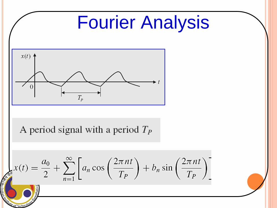
Fourier Analysis

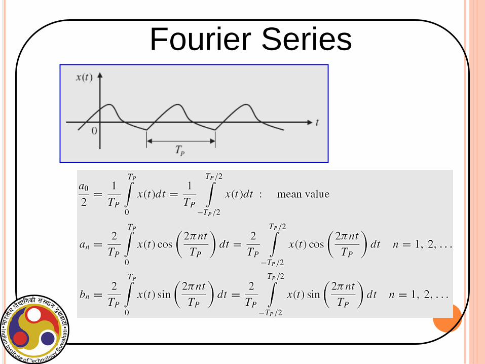
Fourier Series

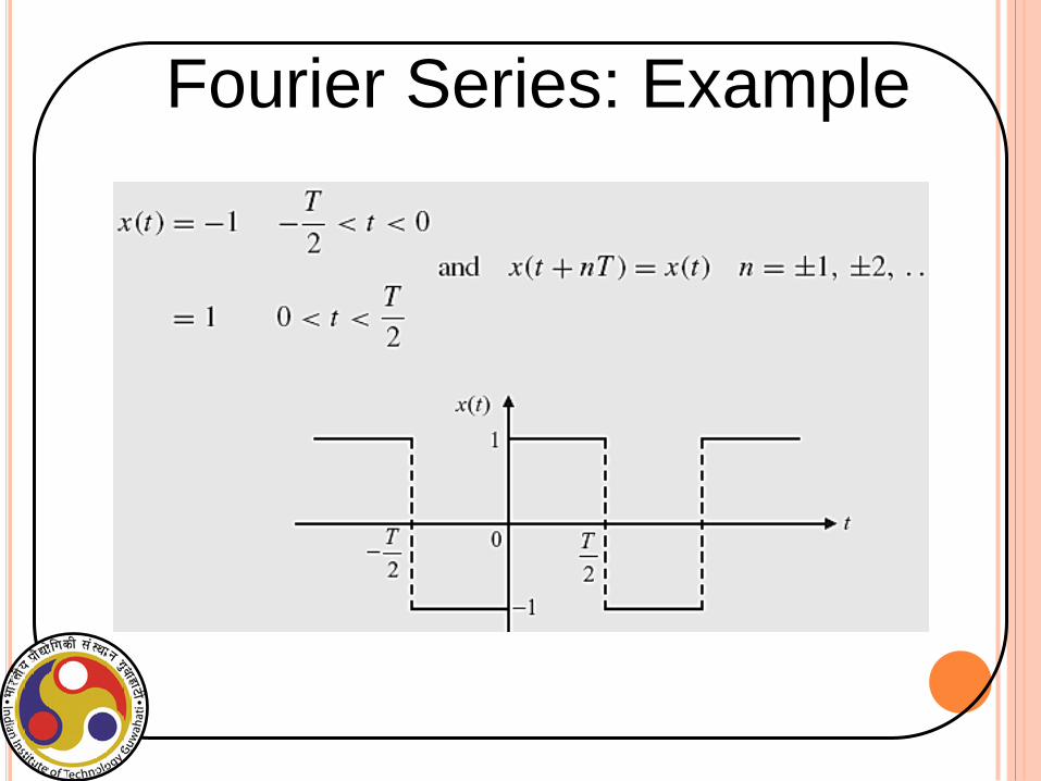
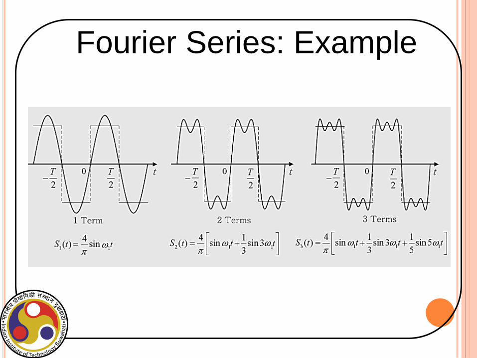
Fourier Series: Example

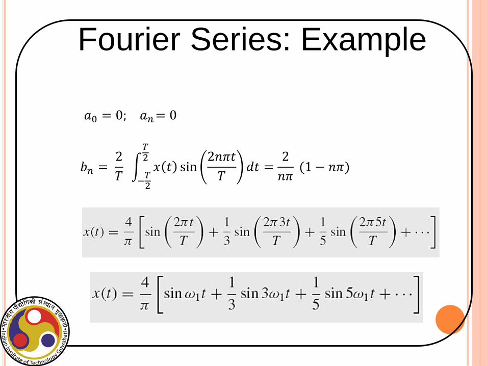
𝑎0 = 0; 𝑎𝑛= 0

𝑏𝑛 = 2

𝑇 𝑥 𝑡 sin

2𝑛𝜋𝑡

𝑇𝑑𝑡 =2

𝑛𝜋

𝑇2

−𝑇2

(1 − 𝑛𝜋)

Fourier Series: Example

Fourier Series: Example

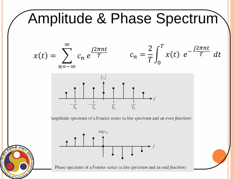
𝑥 𝑡 = 𝑐𝑛 𝑒𝑗2𝜋𝑛𝑡𝑇

∞

𝑛=−∞

𝑐𝑛 =2

𝑇 𝑥 𝑡 𝑒−

𝑗2𝜋𝑛𝑡𝑇 𝑑𝑡

𝑇

0

Amplitude & Phase Spectrum

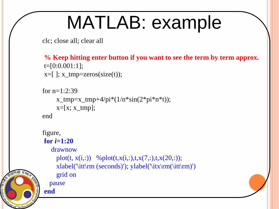
clc; close all; clear all

% Keep hitting enter button if you want to see the term by term approx.

t=[0:0.001:1];

x=[ ]; x_tmp=zeros(size(t));

for n=1:2:39

x_tmp=x_tmp+4/pi*(1/n*sin(2*pi*n*t));

x=[x; x_tmp];

end

figure,

for i=1:20

drawnow

plot(t, x(i,:)) %plot(t,x(i,:),t,x(7,:),t,x(20,:));

xlabel('\itt\rm (seconds)'); ylabel('\itx\rm(\itt\rm)')

grid on

pause

end

MATLAB: example

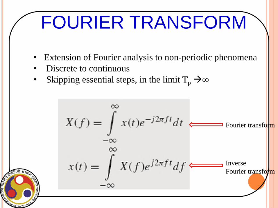
• Extension of Fourier analysis to non-periodic phenomena

• Discrete to continuous

• Skipping essential steps, in the limit Tp ∞

Fourier transform

Inverse

Fourier transform

FOURIER TRANSFORM

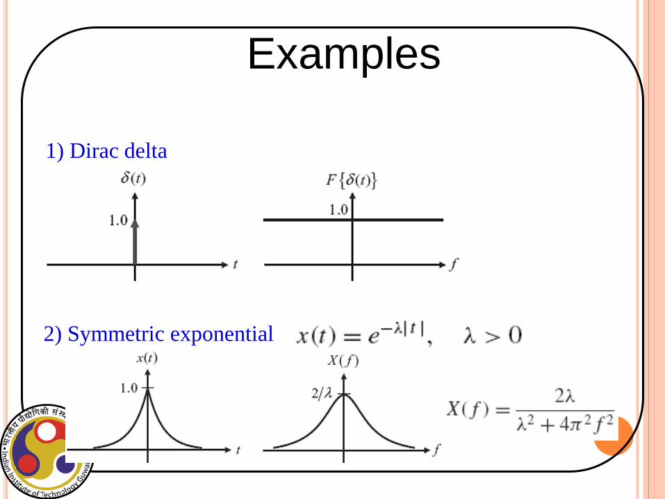
1) Dirac delta

2) Symmetric exponential

Examples

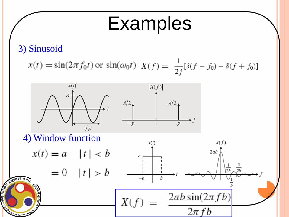
3) Sinusoid

4) Window function

Examples

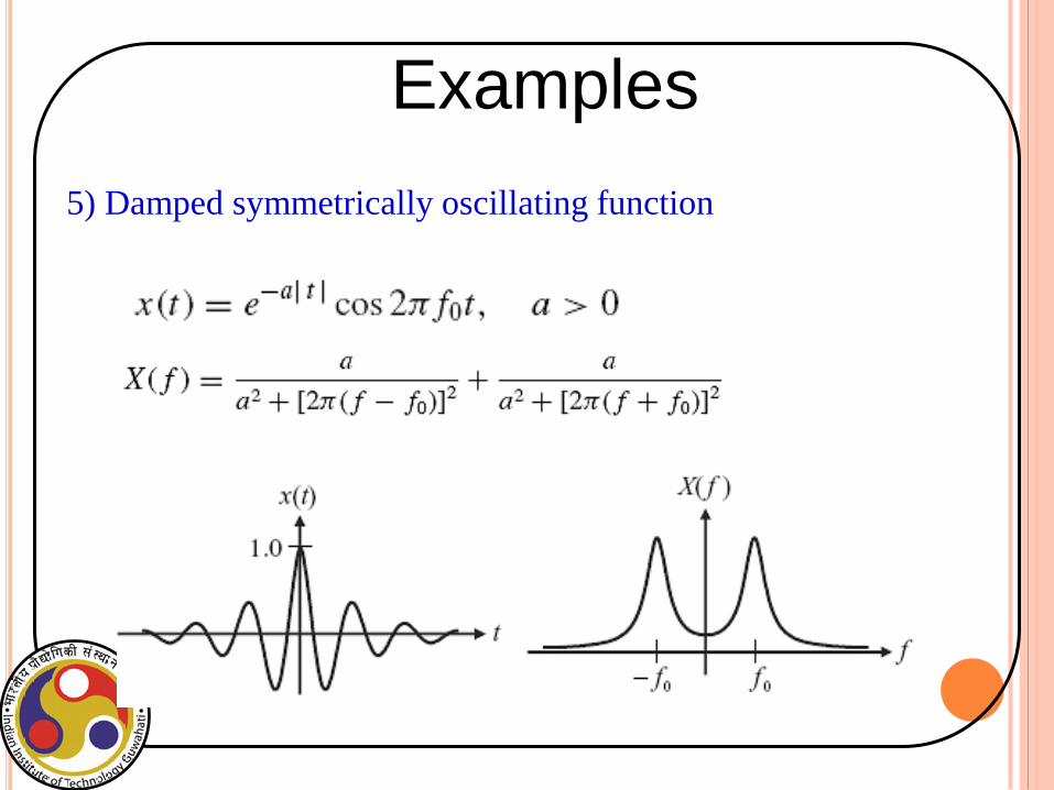
5) Damped symmetrically oscillating function

Examples

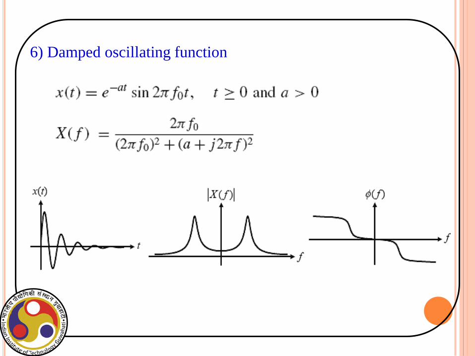
6) Damped oscillating function

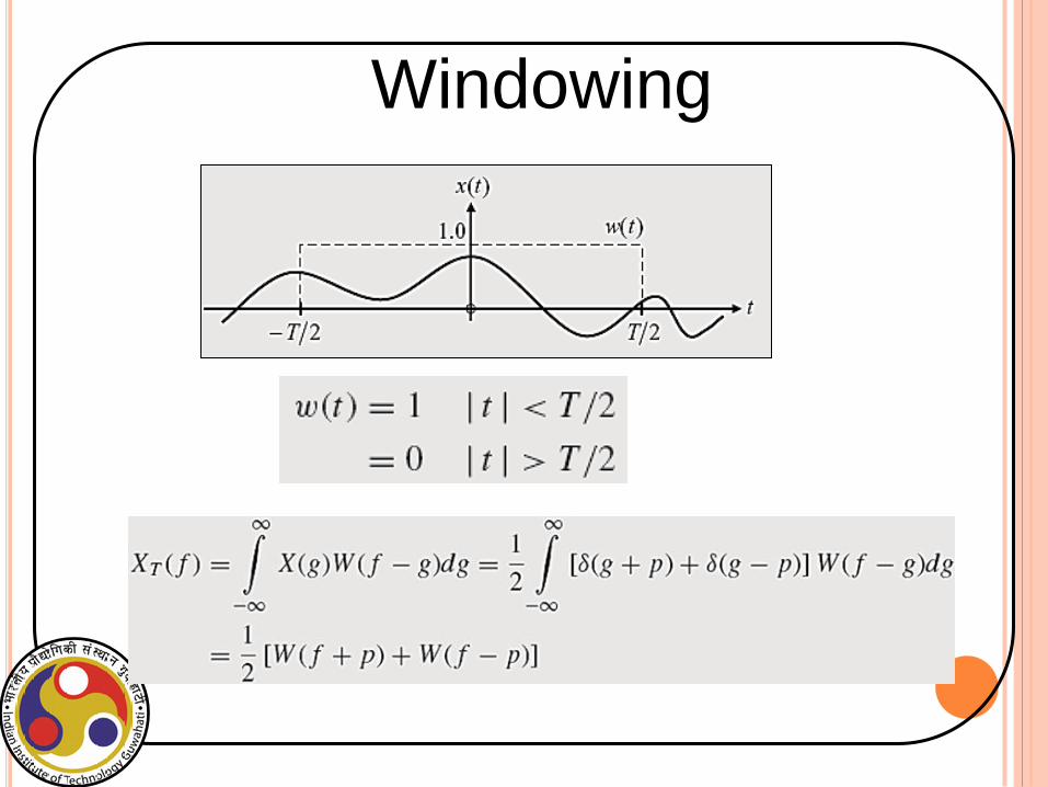
Windowing

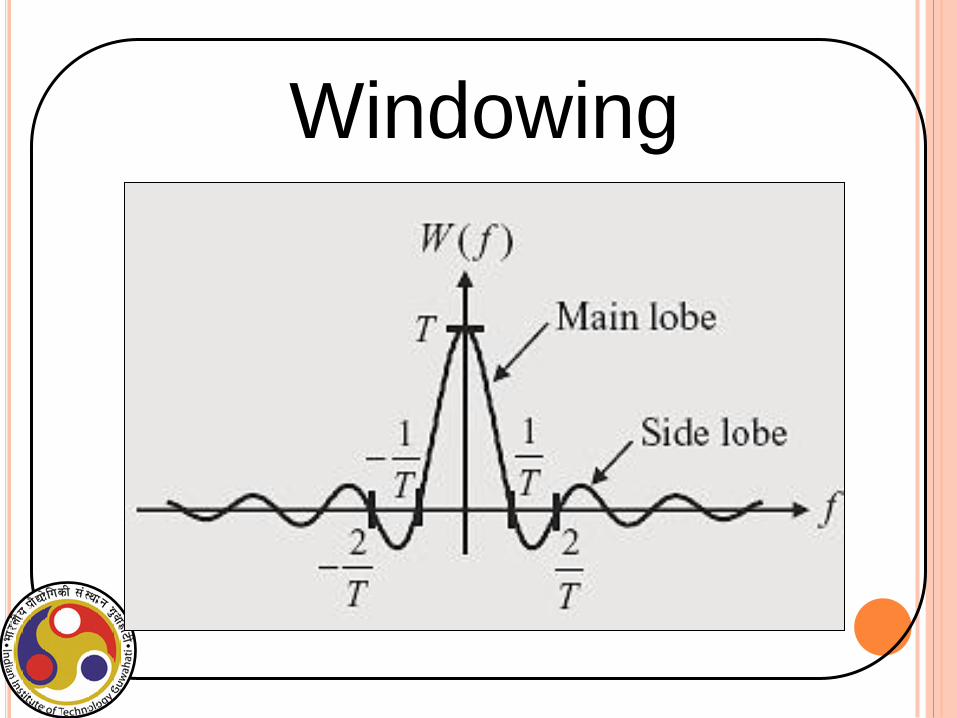
Windowing

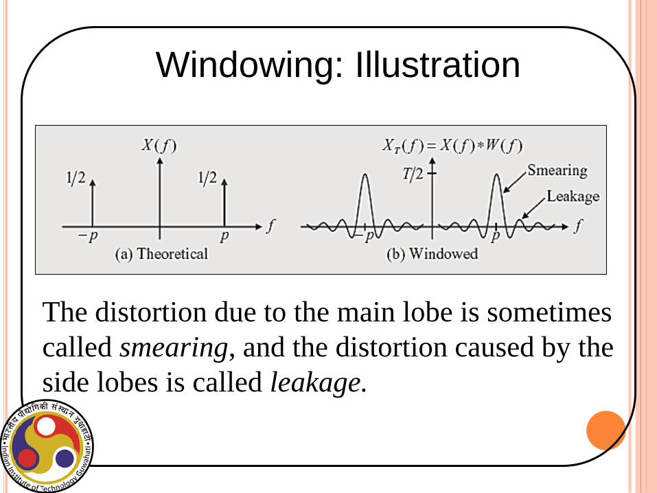
The distortion due to the main lobe is sometimes

called smearing, and the distortion caused by the

side lobes is called leakage.

Windowing: Illustration

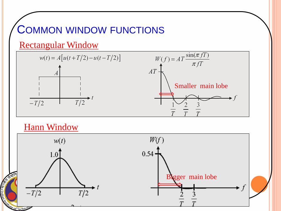
COMMON WINDOW FUNCTIONS

Rectangular Window

Hann Window

Smaller main lobe

Bigger main lobe

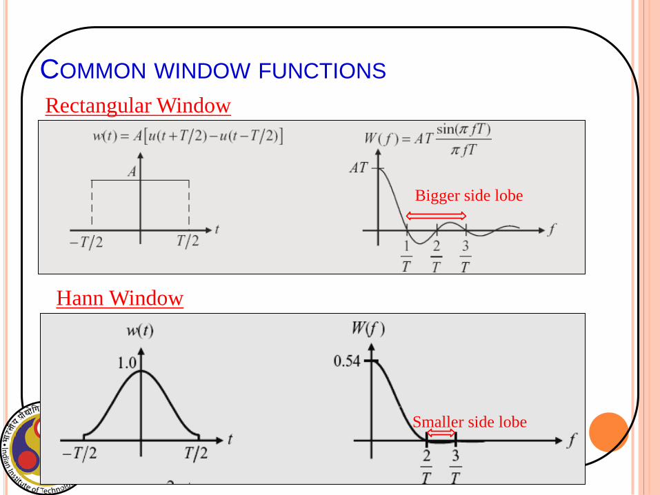
COMMON WINDOW FUNCTIONS

Rectangular Window

Hann Window

Bigger side lobe

Smaller side lobe

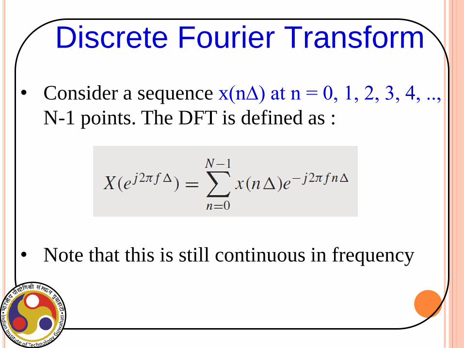
• Consider a sequence x(n∆) at n = 0, 1, 2, 3, 4, ..,

N-1 points. The DFT is defined as :

• Note that this is still continuous in frequency

Discrete Fourier Transform

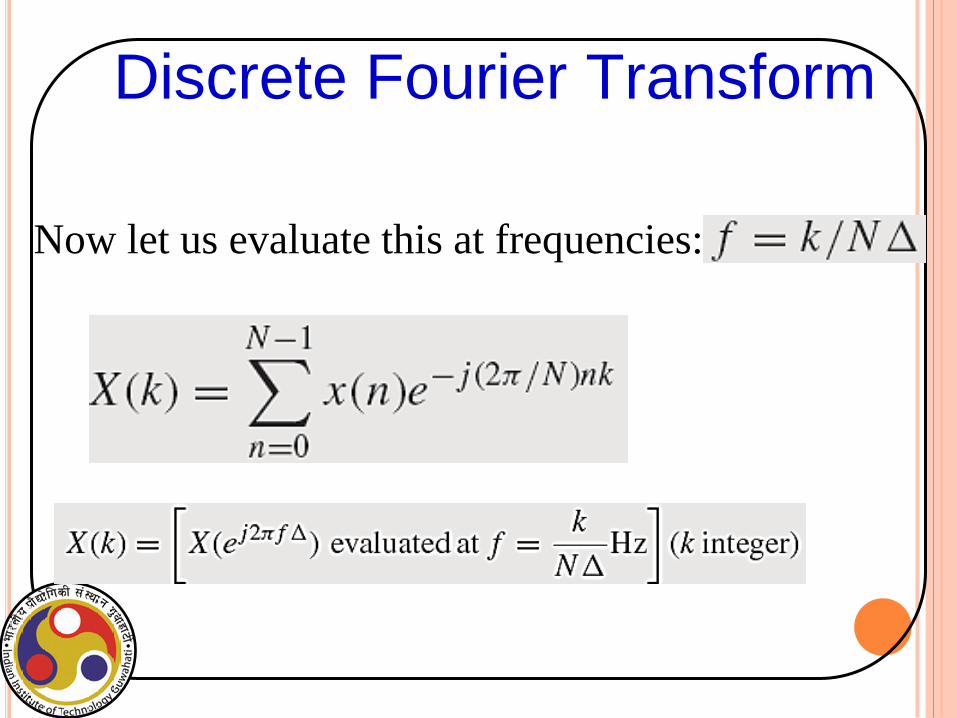
Now let us evaluate this at frequencies:

Discrete Fourier Transform

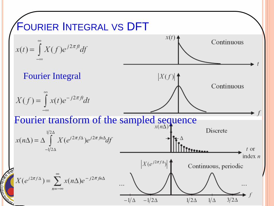
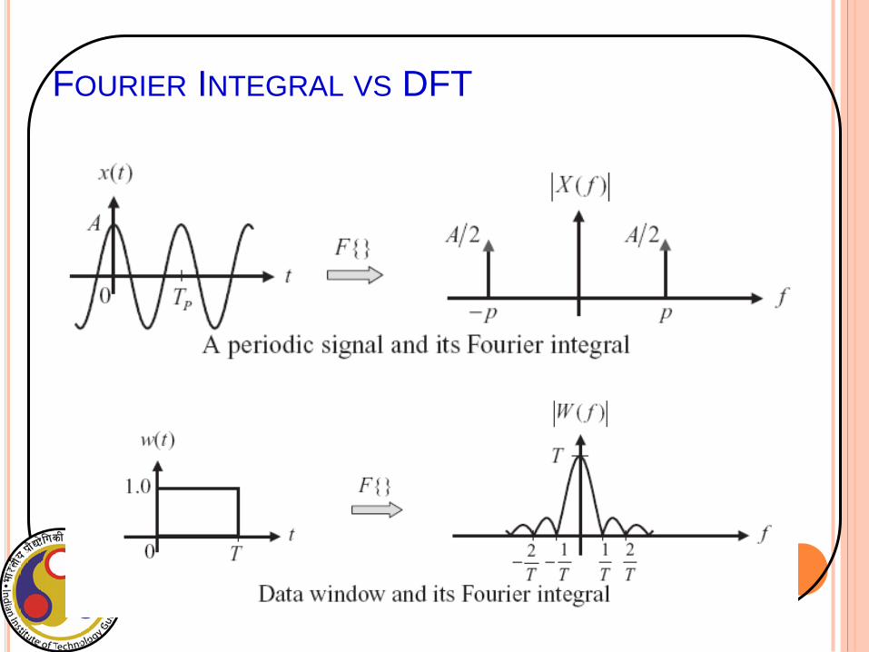
FOURIER INTEGRAL VS DFT

Fourier Integral

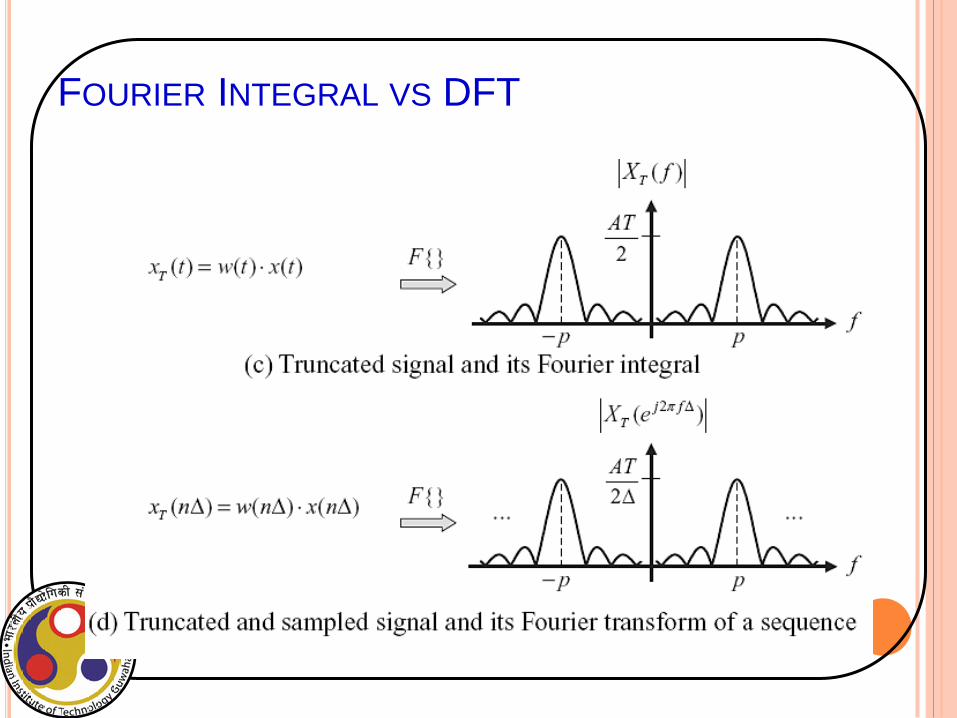
Fourier transform of the sampled sequence

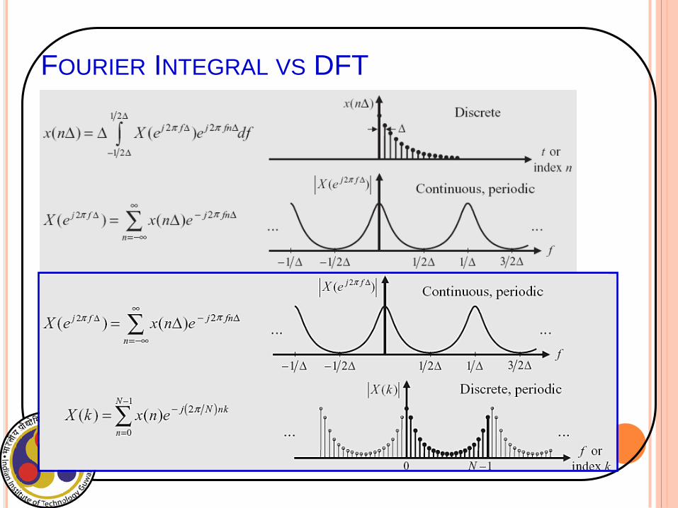
FOURIER INTEGRAL VS DFT

FOURIER INTEGRAL VS DFT

FOURIER INTEGRAL VS DFT

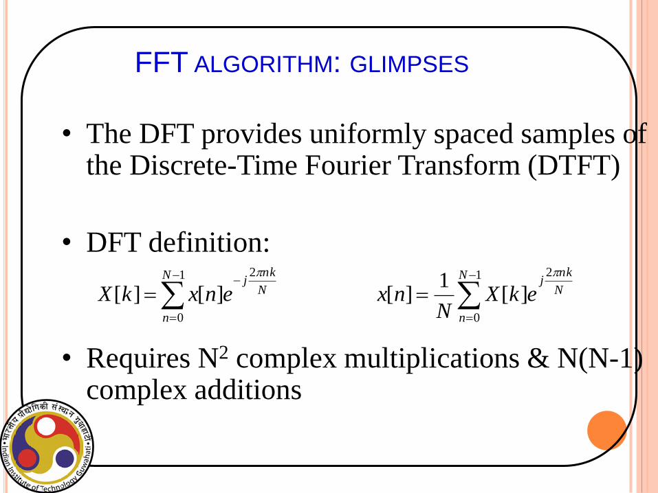
FFT ALGORITHM: GLIMPSES

• The DFT provides uniformly spaced samples of the Discrete-Time Fourier Transform (DTFT)

• DFT definition:

• Requires N2 complex multiplications & N(N-1) complex additions

1

0

2

][][N

n

N

nkj

enxkX

1

0

2

][1

][N

n

N

nkj

ekXN

nx

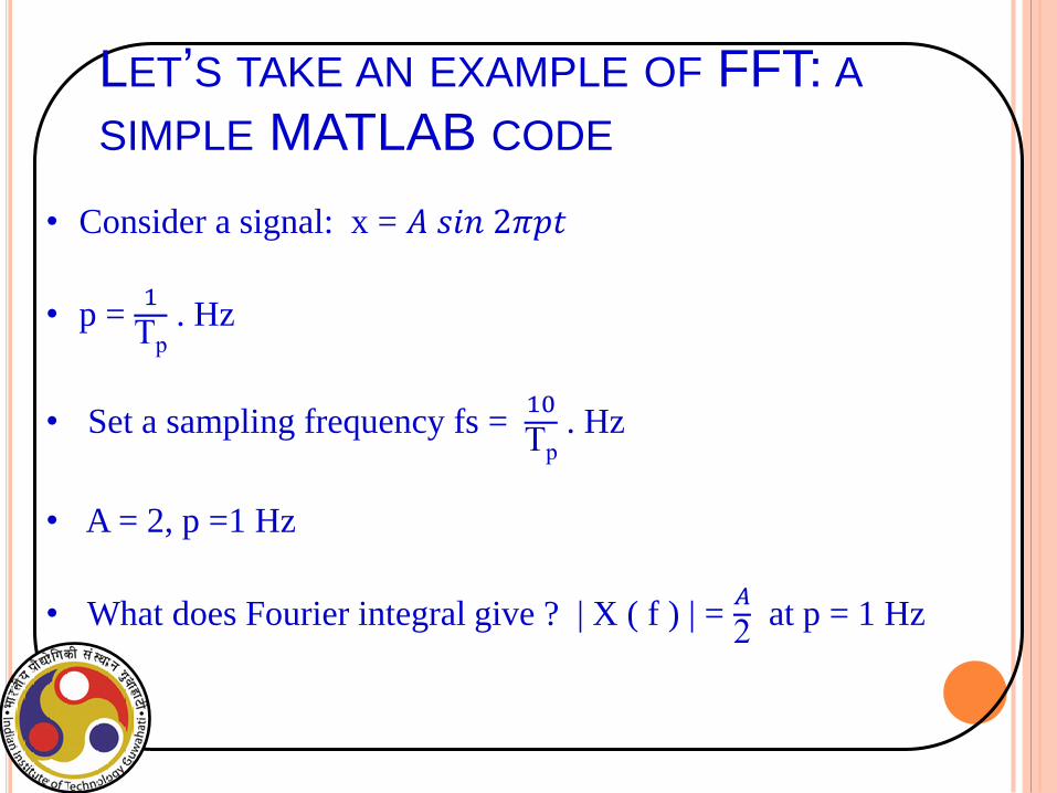
LET’S TAKE AN EXAMPLE OF FFT: A

SIMPLE MATLAB CODE

• Consider a signal: x = 𝐴 𝑠𝑖𝑛 2𝜋𝑝𝑡

• p = 1

Tp . Hz

• Set a sampling frequency fs = 10

Tp . Hz

• A = 2, p =1 Hz

• What does Fourier integral give ? | X ( f ) | = 𝐴

2 at p = 1 Hz

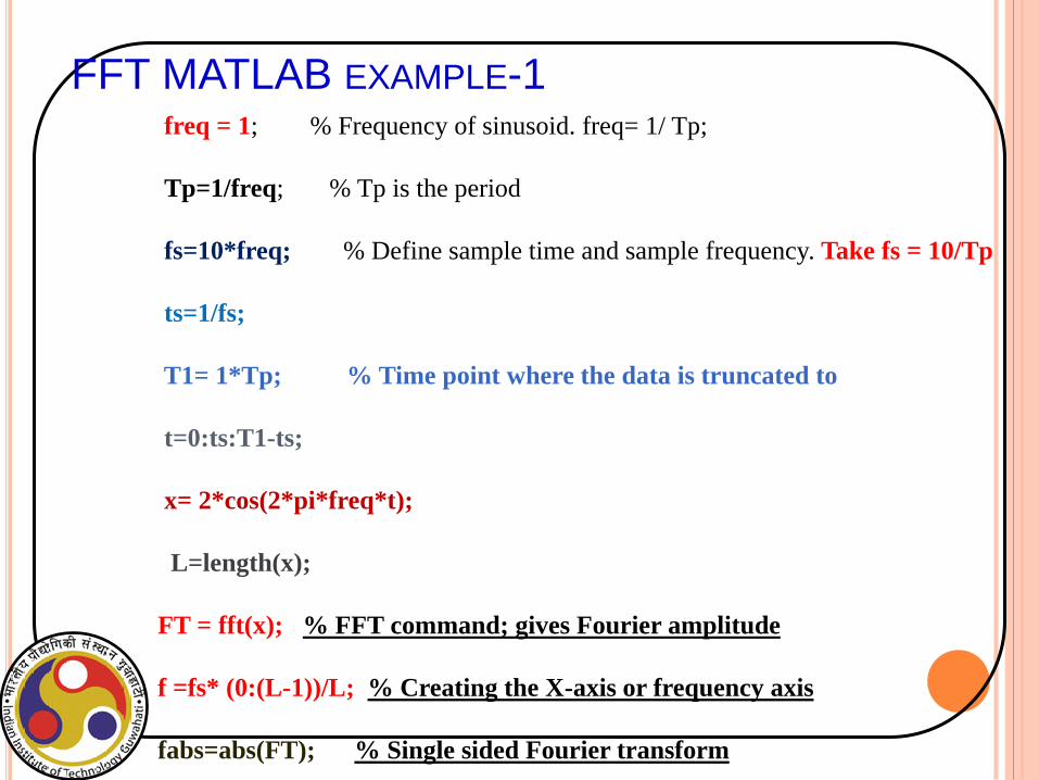
freq = 1; % Frequency of sinusoid. freq= 1/ Tp;

Tp=1/freq; % Tp is the period

fs=10*freq; % Define sample time and sample frequency. Take fs = 10/Tp

ts=1/fs;

T1= 1*Tp; % Time point where the data is truncated to

t=0:ts:T1-ts;

x= 2*cos(2*pi*freq*t);

L=length(x);

FT = fft(x); % FFT command; gives Fourier amplitude

f =fs* (0:(L-1))/L; % Creating the X-axis or frequency axis

fabs=abs(FT); % Single sided Fourier transform

FFT MATLAB EXAMPLE-1

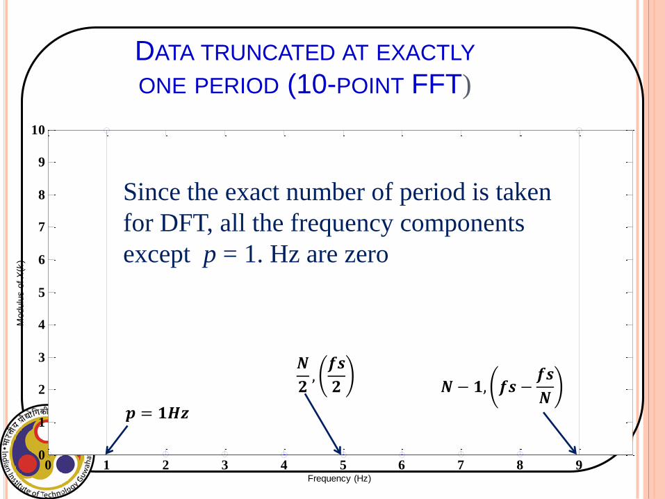
DATA TRUNCATED AT EXACTLY

ONE PERIOD (10-POINT FFT)

0 1 2 3 4 5 6 7 8 90

1

2

3

4

5

6

7

8

9

10

Frequency (Hz)

Modulu

s o

f X

(k)

Since the exact number of period is taken

for DFT, all the frequency components

except p = 1. Hz are zero

𝒑 = 𝟏𝑯𝒛

𝑵

𝟐,𝒇𝒔

𝟐

𝑵− 𝟏, 𝒇𝒔 −𝒇𝒔

𝑵

0 2 4 6 8 100

10

20

30

40

50

60

Frequency (Hz)

Mo

du

lus

of

X(k

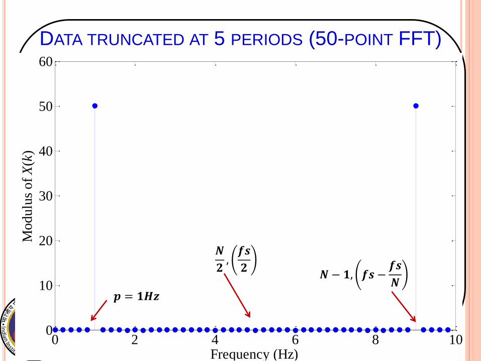
)DATA TRUNCATED AT 5 PERIODS (50-POINT FFT)

𝒑 = 𝟏𝑯𝒛

𝑵

𝟐,𝒇𝒔

𝟐

𝑵− 𝟏, 𝒇𝒔 −𝒇𝒔

𝑵

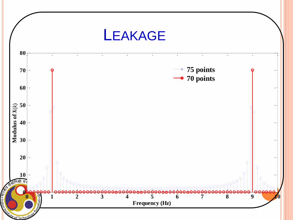
LEAKAGE

0 1 2 3 4 5 6 7 8 9 100

10

20

30

40

50

60

70

80

Frequency (Hz)

Mo

du

lus

of X

(k)

75 points

70 points

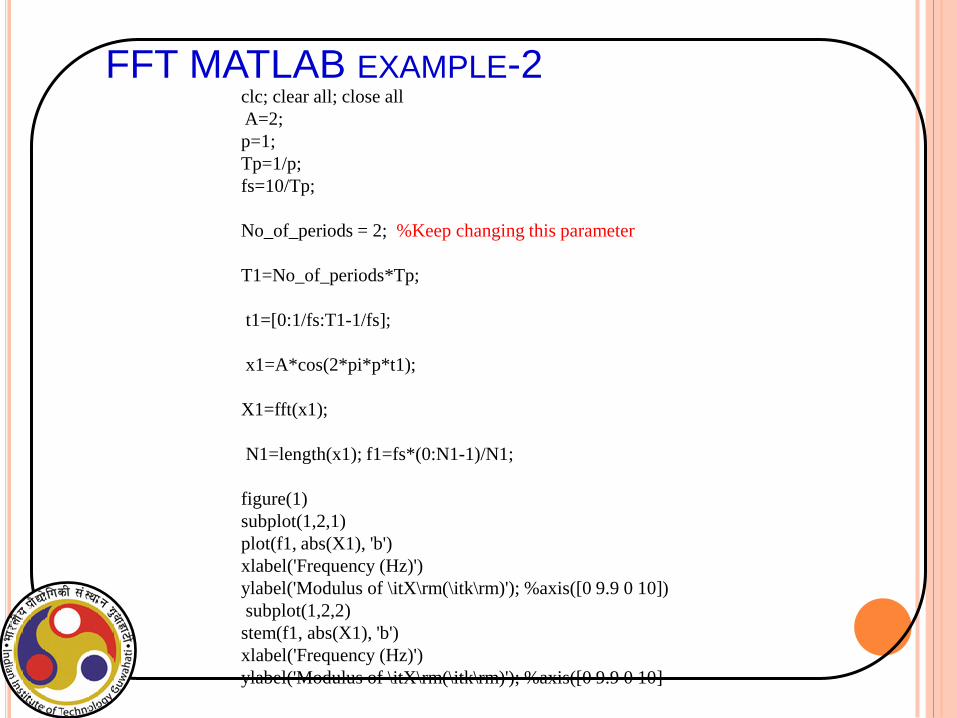
FFT MATLAB EXAMPLE-2 clc; clear all; close all

A=2;

p=1;

Tp=1/p;

fs=10/Tp;

No_of_periods = 2; %Keep changing this parameter

T1=No_of_periods*Tp;

t1=[0:1/fs:T1-1/fs];

x1=A*cos(2*pi*p*t1);

X1=fft(x1);

N1=length(x1); f1=fs*(0:N1-1)/N1;

figure(1)

subplot(1,2,1)

plot(f1, abs(X1), 'b')

xlabel('Frequency (Hz)')

ylabel('Modulus of \itX\rm(\itk\rm)'); %axis([0 9.9 0 10])

subplot(1,2,2)

stem(f1, abs(X1), 'b')

xlabel('Frequency (Hz)')

ylabel('Modulus of \itX\rm(\itk\rm)'); %axis([0 9.9 0 10]

EXTRA

8/2

8/2

017

32

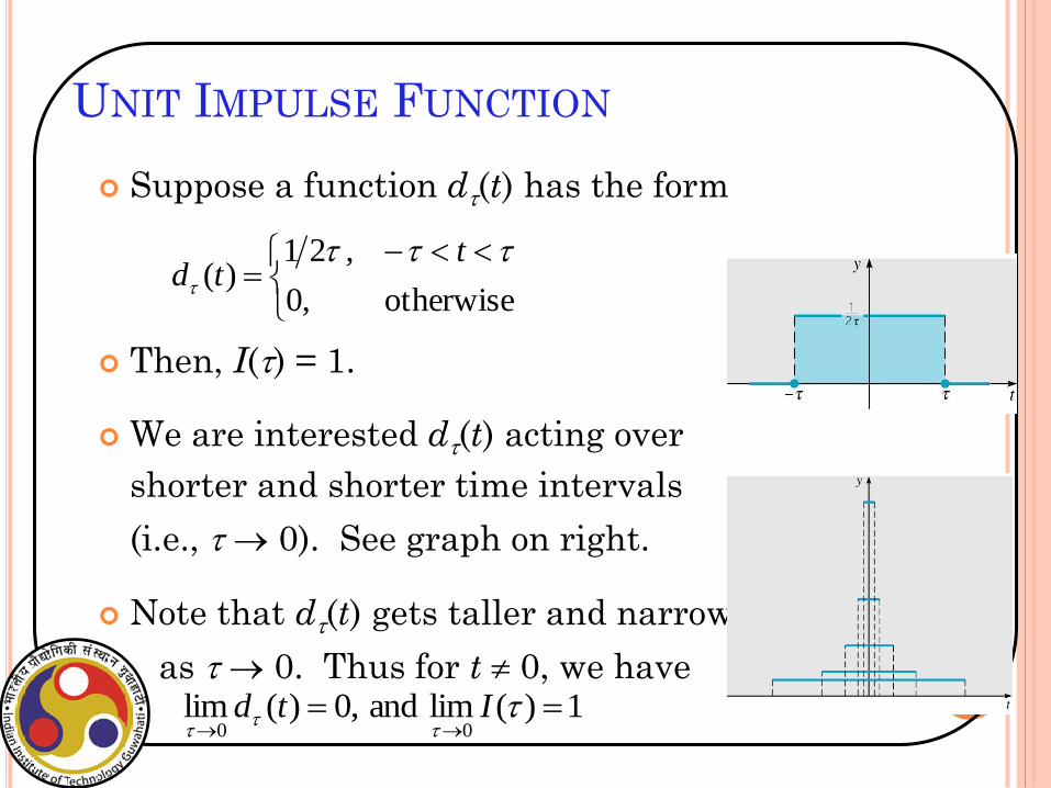
UNIT IMPULSE FUNCTION

Suppose a function d(t) has the form

Then, I() = 1.

We are interested d(t) acting over

shorter and shorter time intervals

(i.e., 0). See graph on right.

Note that d(t) gets taller and narrower

as 0. Thus for t 0, we have

otherwise,0

,21)(

ttd

1)(limand,0)(lim00

Itd

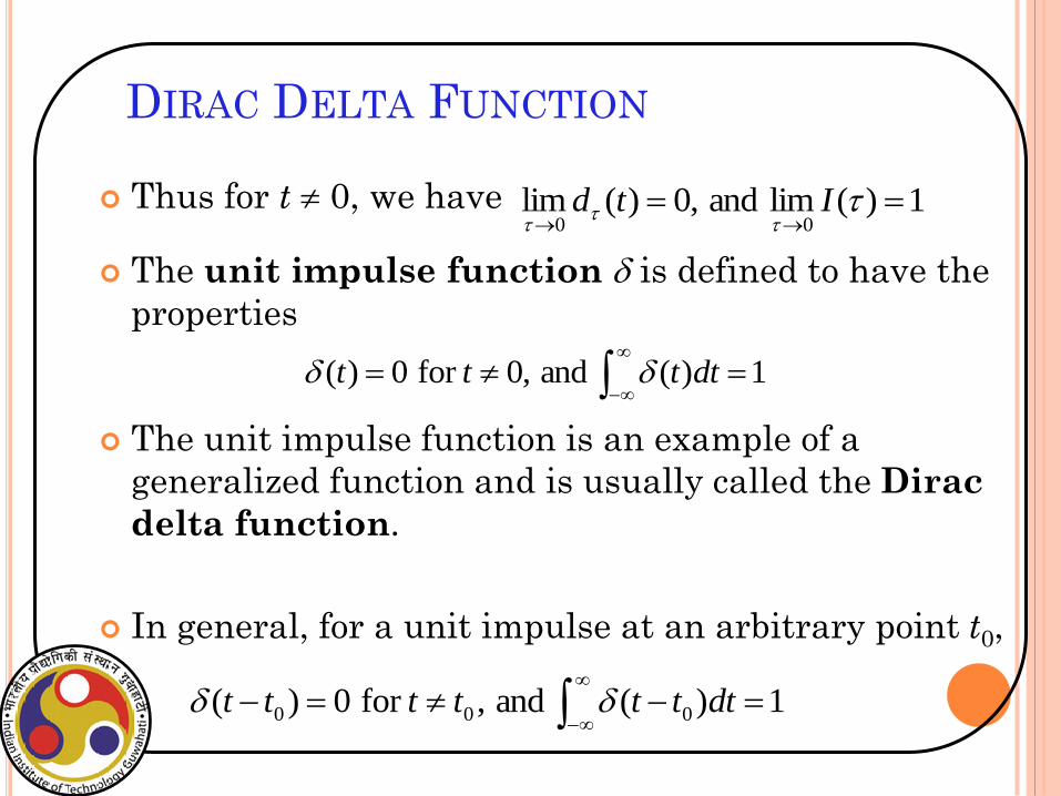
DIRAC DELTA FUNCTION

Thus for t 0, we have

The unit impulse function is defined to have the

properties

The unit impulse function is an example of a

generalized function and is usually called the Dirac

delta function.

In general, for a unit impulse at an arbitrary point t0,

1)(limand,0)(lim00

Itd

1)(and,0for 0)(

dtttt

1)(and,for 0)( 000

dttttttt

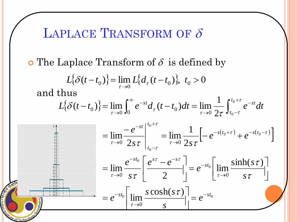
LAPLACE TRANSFORM OF

The Laplace Transform of is defined by

and thus

0,)(lim)( 000

0

tttdLttL

00

0

0

00

0

0

0

0

)cosh(lim

)sinh(lim

2lim

2

1lim

2lim

2

1lim)(lim)(

0

00

00

000

00

stst

stssst

tsts

t

t

st

t

t

stst

es

sse

s

se

ee

s

e

eess

e

dtedtttdettL

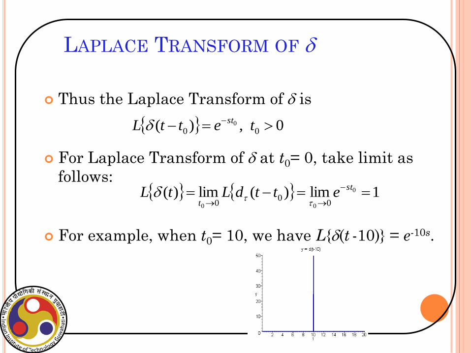
LAPLACE TRANSFORM OF

Thus the Laplace Transform of is

For Laplace Transform of at t0= 0, take limit as

follows:

For example, when t0= 10, we have L{(t -10)} = e-10s.

0,)( 000

tettL

st

1lim)(lim)( 0

00 00

0

st

tettdLtL