CE 498/698 and ERS 685 (Spring 2004)

Lecture 11 1

Lecture 11: Control-Volume Approach (steady-state)

CE 498/698 and ERS 685

Principles of Water Quality Modeling

CE 498/698 and ERS 685 (Spring 2004)

Lecture 11 2

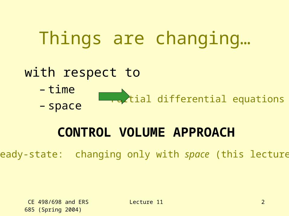
Things are changing…

with respect to– time– space

Partial differential equations

CONTROL VOLUME APPROACH

Steady-state: changing only with space (this lecture)

CE 498/698 and ERS 685 (Spring 2004)

Lecture 11 3

Completely Mixed Lake Model

vAckVcccEQcQcWdtdc

V outin 12

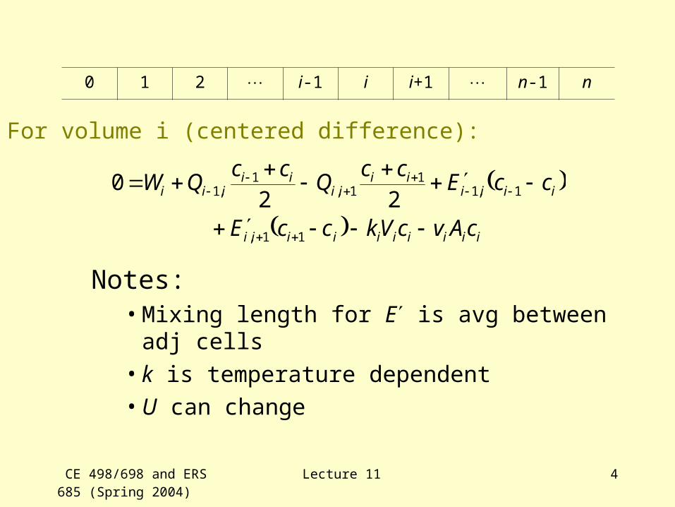
For volume i:

iiiiiiiiii

iiiiii

iiii

iii

cAvcVkccE

ccEcc

Qcc

QW

11,

1,11

1,1

,1

22

0

0 1 2 i-1 i i+1 n-1 n

0

CE 498/698 and ERS 685 (Spring 2004)

Lecture 11 4

For volume i (centered difference):

iiiiiiiiii

iiiiii

iiii

iii

cAvcVkccE

ccEcc

Qcc

QW

11,

1,11

1,1

,1

22

0

Notes:• Mixing length for E is avg between adj cells• k is temperature dependent• U can change

0 1 2 i-1 i i+1 n-1 n

CE 498/698 and ERS 685 (Spring 2004)

Lecture 11 5

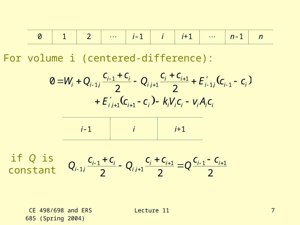
For volume i (centered-difference):

iiiiiiiiii

iiiiii

iiii

iii

cAvcVkccE

ccEcc

Qcc

QW

11,

1,11

1,1

,1

22

0

i-1 i i+1

21

,1ii

ii

ccQ

21

1,

ii

ii

ccQ

0 1 2 i-1 i i+1 n-1 n

CE 498/698 and ERS 685 (Spring 2004)

Lecture 11 6

For volume i (backward difference):

iiiiiiiiii

iiiiiiiiiii

cAvcVkccE

ccEcQcQW

11,

1,11,1,1

0

i-1 i i+1

1,1 iii cQiii cQ 1,

0 1 2 i-1 i i+1 n-1 n

CE 498/698 and ERS 685 (Spring 2004)

Lecture 11 7

For volume i (centered-difference):

iiiiiiiiii

iiiiii

iiii

iii

cAvcVkccE

ccEcc

Qcc

QW

11,

1,11

1,1

,1

22

0

i-1 i i+1

222111

1,1

,1

iiii

iiii

ii

ccQ

ccQ

ccQ

0 1 2 i-1 i i+1 n-1 n

if Q isconstant

CE 498/698 and ERS 685 (Spring 2004)

Lecture 11 8

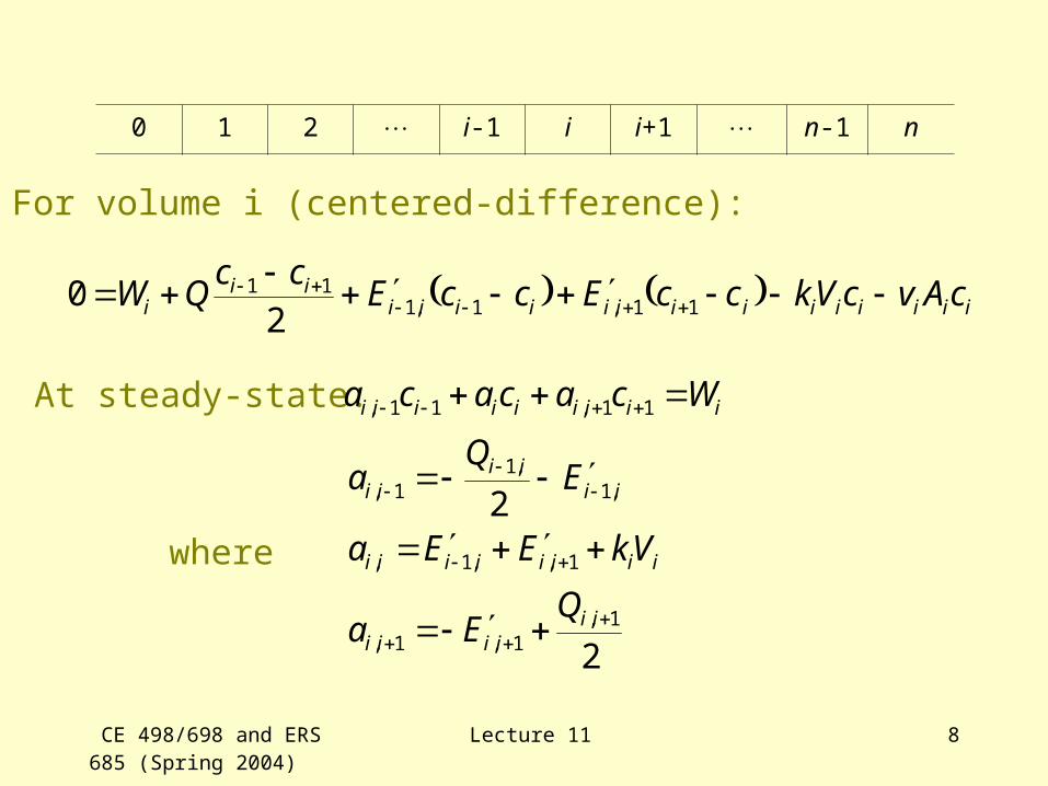
For volume i (centered-difference):

0 1 2 i-1 i i+1 n-1 n

iiiiiiiiiiiiiiii

i cAvcVkccEccEcc

QW

11,1,111

20

At steady-state: iiiiiiiii Wcacaca 11,11,

where

2

2

1,1,1,

1,,1,

,1,1

1,

iiiiii

iiiiiiii

iiii

ii

QEa

VkEEa

EQ

a

CE 498/698 and ERS 685 (Spring 2004)

Lecture 11 9

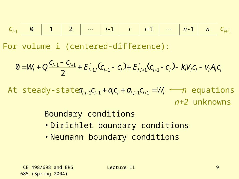
For volume i (centered-difference):

0 1 2 i-1 i i+1 n-1 n

iiiiiiiiiiiiiiii

i cAvcVkccEccEcc

QW

11,1,111

20

At steady-state: iiiiiiiii Wcacaca 11,11, n equations

n+2 unknowns

ci-1 ci+1

Boundary conditions• Dirichlet boundary conditions• Neumann boundary conditions

CE 498/698 and ERS 685 (Spring 2004)

Lecture 11 10

For loading at volume 1:

22,111,100,11 cacacaW

0 1 n n+1

22,111,11 cacaW

00,11 caW

openboundaries

CE 498/698 and ERS 685 (Spring 2004)

Lecture 11 11

For loading at volume 1: 00,111 caWW

0 1 n n+1

For loading at volume n: 11, nnnnn caWW

n equationsn unknowns

solve for c’s

openboundaries

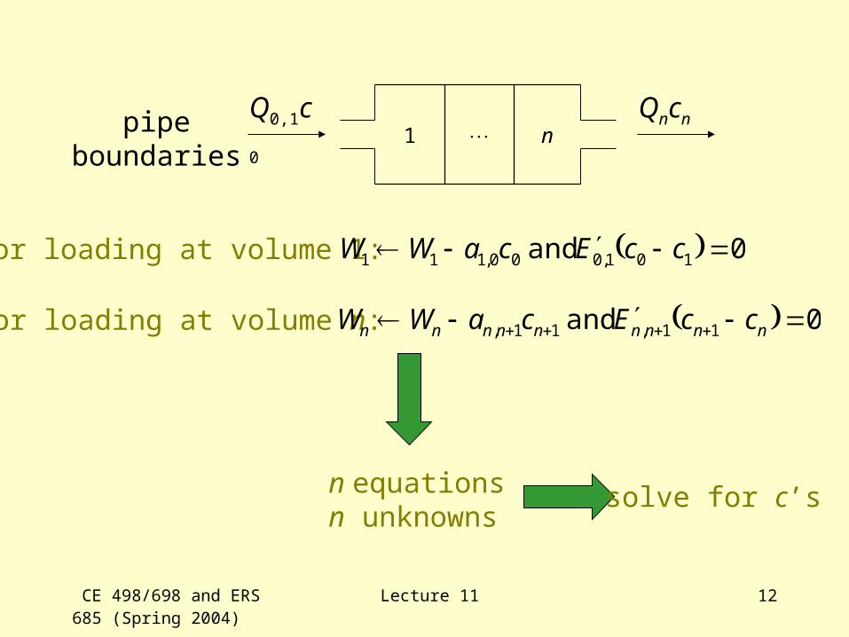
CE 498/698 and ERS 685 (Spring 2004)

Lecture 11 12

For loading at volume 1: 0 and 101,000,111 ccEcaWW

For loading at volume n: 0 and 11,11, nnnnnnnnn ccEcaWW

n equationsn unknowns

solve for c’s

pipeboundaries

n1Q0,1c0 Qncn

CE 498/698 and ERS 685 (Spring 2004)

Lecture 11 13

Numerical dispersion

Example 11.1:Backward differences

Example 11.3:Centered differences

Figure E11.1-2

Figure E11.3

CE 498/698 and ERS 685 (Spring 2004)

Lecture 11 14

Numerical dispersionkc

dxcd

Edxdc

U 2

2

0

Taylor-series expansion

2

21

2 dxcdx

x

cc

dxdc ii

2

21

2 dxcdx

dxdc

x

cc ii

!3!2

3

3

32

2

2

1

xdxcdx

dxcd

xdxdc

cc ii

Backwarddifference

kcdxcd

Edxcdx

dxdc

U

2

2

2

2

20

CE 498/698 and ERS 685 (Spring 2004)

Lecture 11 15

Numerical dispersionkc

dxcd

Edxdc

U 2

2

0

Taylor-series expansion

!3!2

3

3

32

2

2

1

xdxcdx

dxcd

xdxdc

cc ii

2

21

2 dxcdx

x

cc

dxdc ii

2

21

2 dxcdx

dxdc

x

cc ii

Backwarddifference

kcdxdc

Udxcd

Ux

E

2

2

20

numerical dispersion: Ux

En 2 does not occur w/

centered difference

CE 498/698 and ERS 685 (Spring 2004)

Lecture 11 16

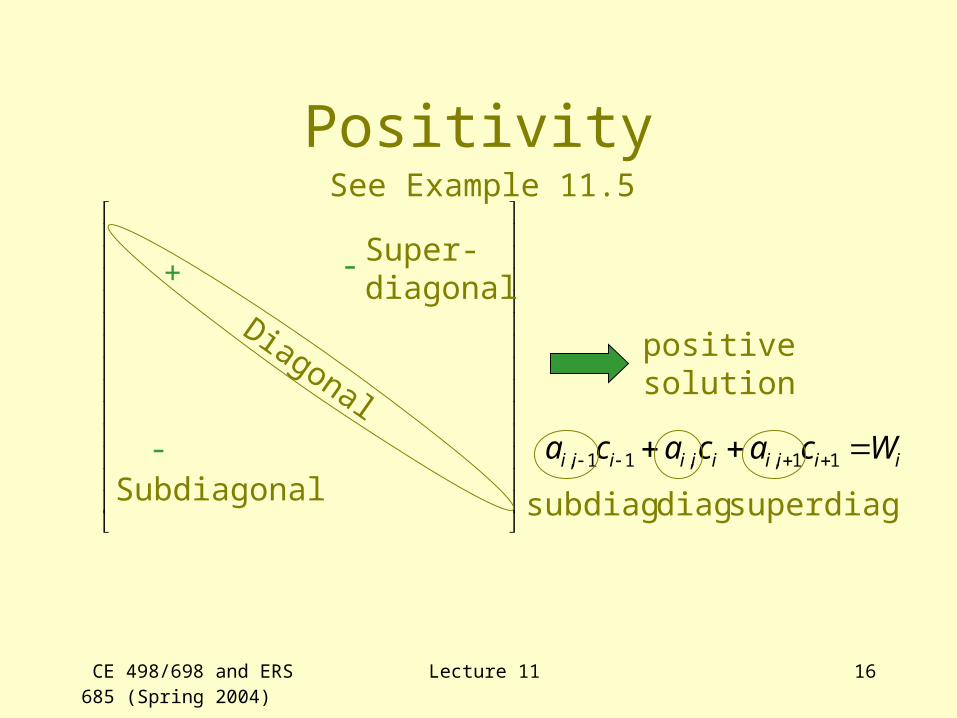
PositivitySee Example 11.5

Diagonal

Super-diagonal

Subdiagonal-

-+

positivesolution

iiiiiiiiii Wcacaca 11,,11,

subdiag diag superdiag

CE 498/698 and ERS 685 (Spring 2004)

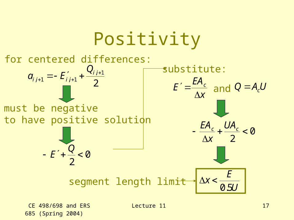
Lecture 11 17

Positivity

21,

1,1,

iiiiii

QEa

must be negative to have positive solution

02

QE

substitute:

x

EAE c

and UAQ c

02

cc UA

x

EA

UE

x5.0

for centered differences:

segment length limit

CE 498/698 and ERS 685 (Spring 2004)

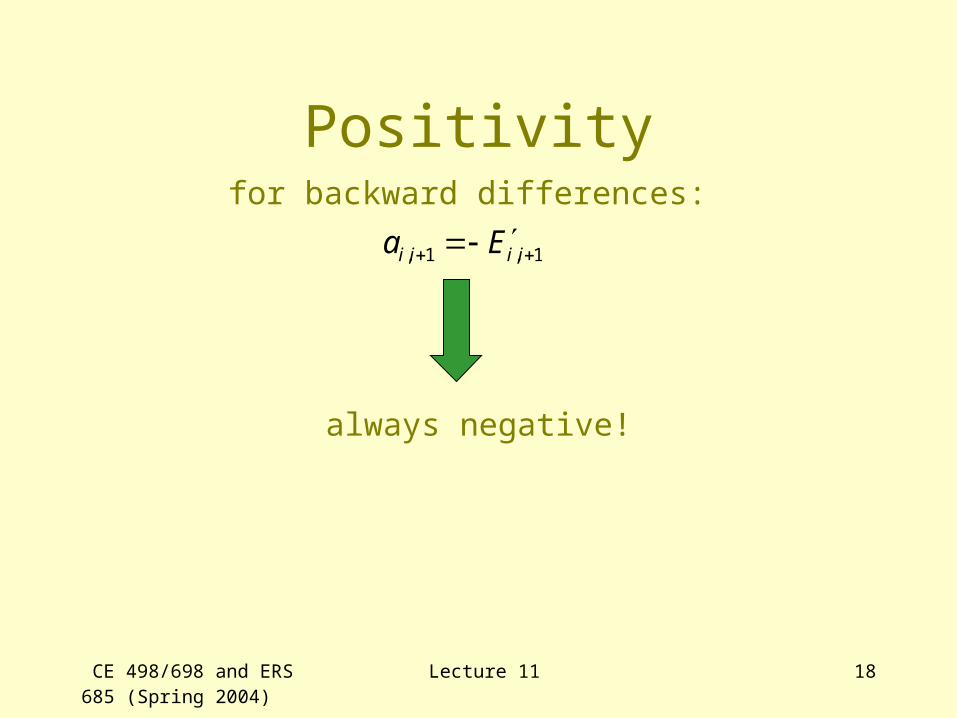
Lecture 11 18

Positivity

1,1, iiii Ea

for backward differences:

always negative!

CE 498/698 and ERS 685 (Spring 2004)

Lecture 11 19

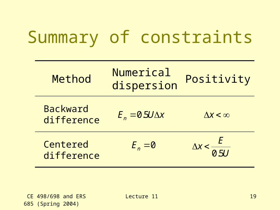
Summary of constraints

Centered difference

Backward difference

PositivityNumerical dispersion

Method

xUEn 5.0 x

0nEUE

x5.0

CE 498/698 and ERS 685 (Spring 2004)

Lecture 11 20

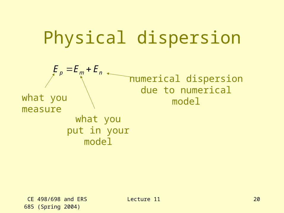
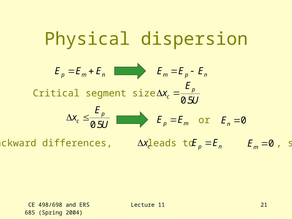
Physical dispersion

nmp EEE

what youmeasure

what youput in your

model

numerical dispersiondue to numerical

model

CE 498/698 and ERS 685 (Spring 2004)

Lecture 11 21

Physical dispersion

nmp EEE npm EEE

U

Ex pc 5.0Critical segment size

For backward differences, leads to , sonp EE cx 0mE

U

Ex pc 5.0

mp EE 0nEor