Embed Size (px)
Citation preview
CE 394K.2 Hydrology
Homework Problem Set #1
Due Thurs Feb 22
Problems in "Applied Hydrology"
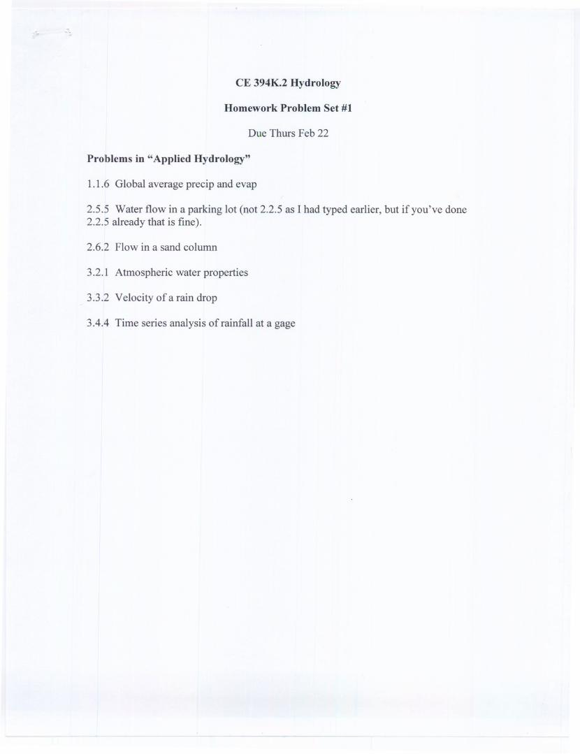
1.1.6 Global average precip and evap
2.5.5 Water flow in a parking lot (not 2.2.5 as I had typed earlier, but if you've done2.2.5 already that is fine).
2.6.2 Flow in a sand column
3.2.1 Atmospheric water properties
3.3.2 Velocity of a rain drop
3.4.4 Time series analysis of rainfall at a gage
.._--
Pt · ~.5 x 10N x 1.02t-1980
The annual per capita water use is 6.8 m'/day . 2,~82 x 10-' km'/year.It per capita water use remains constant, the total water use tor year t maybe calculated as .
Pt x 2,!l82 x 10-' km'/year. ~.5 x 10' x 1.02t-1980 x 2,~82
x 10-' km'/year . 11,169x 1.02t-1980km'/year
Shortage ot tresh water will occur .whenannual water use exceeds the47,000 kmt ot surtace and subsurtace run'ott (Table 1.1.2 ot the textbook)available tor use on an annual basis, that Is when.
11,169 x 1.02t-1980 > 117,000
or, atter some algebra, when
t ) 1980 + 1n (~7,OOO/",'69) / 1n 1.02 · 2,052.6
Theretore, shortage will occur in the year 2053.
1.1.5.
The areas or land and ocean are (Table 1.1.2 or the textbook),respecti vely, 1118,800,000 and 361,300,000 km2. The annual precipi tat~onvalues (Table 1.1.2 or the textbook) are 119,000 kmt/year over the land and!l58,OOOkmt/year over the ocean. The slobal averase precipitationP may becalculated as .
P · (119,OOO+!l58,OOO) / (1118,800,000+361,300,000) km/year
· 1.131 x '.0-3 km/year · 113.1 cm/ye8J".
Annual evaporation equals 72,000 km'/year over the .land and 505,000km' /year over the ocean. The slobal averase evaporation E may be calculatedas
E · (72,000+505,000) / (1118,800,000+361,300,000)km/year . 113.1 em/year
which Is equal to the global average precipitation, as expected. Globalevaporation and precipi.tation must be equal since, trom the viewpoint ot theatmospheric sUbsystem ot the hydrologic cycle, evaporation and precipitationconstitute the only input and output, respectively.
'3The average precipi tation Is equal (Table 1.1.2 ot
in/year over the land and ~O in/year over the ooean.the textbook) to 31The global average
1-2

rpreci pi tationP may be calcul ated as a weighted average of these val ues,
P · (31 x 1l18,800,000 + 50 x 361,300,000) / (1 lI8,800,000+361 ,300,000)
· lIlI in/year.
The global average evaporation E may be calculated in a similar way,
E · (19 x 148,800,000 + 55 x 361,300,000) / (148,800,000+361,300,000)
· 4~ in/year
, which is equal to the global average precipi tation, as expected.
The left side of the differential equation
K(dQ/dt) + Q(t) · let)
can be converted into an exact deri vati ve mul tlplying by the factor et/K.The equation may thus be written as
Ket/K (dQ/dt) + et/K Q(t) . et/K let) for t ~ 0
so that
d(Ket/K Q)Idt . et/~ let)
and, after integration
t .
Ket/K Q . J e~/K I(~) d~ + C for t ~ 0o
where C stands for an integration constant. Then
tQ. 1/K e-t/K {J e~/K l(~) dt + C} for t ~ 0
o
To determine the constant C, we may substitute t. 0 in the previousequation, obtaining
QO · Q(O) · C/K
so that C · KQO' Therefore
t
Q · J 1/K e (-r- t) /K I ( ~) d t + QOo
e-t/K for t i= 0 (1.3.1-1)
1"-3
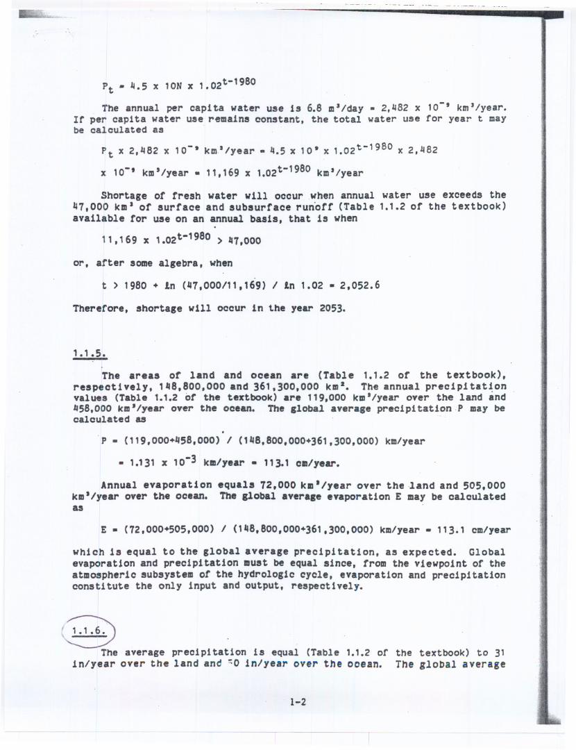
that Eq. (2.2.~-1) reduoes to
11 - Q1· 0 (2.2.~-2)
The average annual inflow is
11 · average annual runoff + preoipitatlon on the reservoir
· 0.33 m x (500 x 109 m2) + 0.90 m x (1,700 x 10~ m2)
· 180,300,000 mI
Not1oe that total preoipitation on the reservoir is added to surfaoe runoff,sinoe the problem speoifies the looation of the reservoir at the basinoutlet.
The average annual outflow 1s
Q1 · average annual evaporat10n + average annual withdrawal
· 1.30 m x (1,700 x 10~ m2) +Qd · 22,100,000mJ + Qd
Then, subst! tutlng in Eq. (2.3.11-2)
11 - Q1· 180,300,000 - (22,100,000 + Q«f · 0
so the average annual withdrawal is Qd · 158,200,000 mJ/year.
2.2.5.
As in Problem 2.2.~, the average annual inflow is
11 · average annual runoff + preoipitation on the reservoir
· (13/12.ft) x (200 x 5,280 ftZ) + (35/12 ft) x (200 x.5,280 ft2)
· 6,573,930.000 ft'.
The average annual. outflow is
"61 · average annual evaporation + average annual w1thdrawal
· (50/12 ft) x (200 x 5,280 ft2) + Qd · 762.300.000 ft) + Qd
Then
11 - Q1 · 6,573..930,000 - (762,300,000 + Qd) · 0
so the average annual wi thdrawal 1s
Qd. 5,811.630,000.ft'/year. 133,1116.7 ao.ft/year.-
2-3

~
· So · 0.01 for uniform flow
v - (1.~9/n) R2/3 S}/2 - (1.~9/0.035) x 2.752/3 x 0.011/2 ft/s- 8.35 ft/s
The flow rate is Q . v A · 8.35 x 327 cfs · 2.731 cfs. The crlterlon forfully turbulent flow Is calculated from Eq. (2.5.9a)in the textbook
n6 (RSf)1/2 . 0.0356 (2.75 x 0.0,)'/2 . 3.05 x 10⁻¹⁰
which is larger than 1.9 x 10⁻¹³ so the criterion is satisfied and Hanning'sequation Is applioable.
The area of the channel Is A · (30 + 3 x 1) x 1 ma · 33 m'. The wetted
perimeter Is
P . 30 + 2 x 1 x (1a + 32)1/2 m · 33;16 m
II
so the hydraulic radi us is R · AlP · 33/33.16 · 0.995 m.
The flow velocity is given by Hanning's equation with n · 0.035 and Sf· So -.0.01 for uniform flow
v . (1/n) R2/3 S}/2 . (1/0.035) x 0.9952/3 x 0.01'12 mls · 2.85 m/s
The flow rate Is Q ~ v A · 2.85 x 33 mIls · 9~ mIls. The c~iterlon forfully turbulent flow is calculated from Eq. (2.5.9b) In the textbook
n6 (RSf)1/2. 0.0356 (0.995 x 0.01)'/2 . 1.83 x 10⁻¹⁰
which is larger than 1.1 x 10⁻¹³ 80 the criterion i8 satisfied and Hanning's
equation is applicable. .
§Shallow flow.over a parking lot is equivalent to flow in an infinite
width channel; in this case, the flow can be analyzed in a portion ofchannel of uni t width. For a flow depth of 1 in, the area of this channelportion is A · 1/12 x 1 fta · 0.083 fta. The wetted perimeter correspondsonly to the channel bottom, P · 1 ft, so the hydraulic radius is R · AlP ·0.083/1 ft. 0.083 ft, equal to the flow depth.
.,e flowvelocity is given by Hanning's equation with n · 0.015 and Sf:>.5 J · 0.005 for uniform flow
. . (1.~9/n) R2/3 S}/2 . (1.~9/0.015) x 0.0832/3 x 0.005'/2 ft/s .
2-9
rIf
. 1.311 rtls
The flow rate per unit widthof channel is Q · v A - 1.311 x 0.083 cfs/ft -D~ IH") --- crs/ft. The criterion for fully turbulent flow is calculated from Eq.
(2.5.9a) in the textbook
n6 .(RSr)1/2 - 0.0156 (0.083 x 0.005)1/2 - 2.32 x 10⁻¹³
.which is larger than 1.9 x 10⁻¹³ so the cr1 ter10n is satisfied and Manning'sequation is applicable.
2.5.6.
For a flow depth of 1 em, the area of a unit width channel portion 1s A- 0.01 x 1 m2 - 0.01 mi. The wetted perimeter corresponds only to thechannel bottom, P - 1 m, so the hydraulic radius is R · AlP · 0..01/1 m ·0.01 m, equal to the flow depth.
To check whether Manning's equation is applicable, the cri terion forfully turbulent flow is calculated from Eq. (2.5.9b) in the textbook
n6 (RSf)1/2 . 0.0156 (0.01 x 0.005)'/2. 0.81.x 10-13
which is smaller than 1.1 x 10⁻¹³ so the criterion is not satisfied(although the flow is very close to fully turbulent); Manning's equation is.not applicable and the Darcy-Weisbach equation should be used instead.
The relative roughness £ is computed uSing Eq. (2.5.15) from thetextbook, as a function of the hydraulic radius R . 0.01 m and the Manning'scoefficient n · 0.015, with the factor t · 1 for 51 units. Then
_.R'/6/[~n(2g)1/2]£ · 3 x 10 · 0.0511
The flow velocity v and the Darcy-Weisbach friction factor f have to becalculated 1n an iterative fashion. For a given value of v, the Reynolds
number Re can be computed using E% (2.5.10) from the textbook. For a valueof the kinematic viscosity v · 10- mIls, we have
Re · ~vR/v . !Iv x 0.01/10~6 · ~O,OOOv (2.5.6-1)
The friction factor r can then be updated using the modified Moodydiagram in Fig. 2.5.1 of the textbook or the Colebrook-Whi te equation (Eq.2.5.13 from the textbook). In this case the latter method w111 be preferredsinceit is more accurate and easier to implementin a computer code. Forflow in the transition zone, .
1/1f · -2 10g10[£/3 + 2.5/Re x 1/1f] ·· -2 10g,0[0.0511/3 + 2.5/Re x 111t] (2.5.6-2)
2-10
q · KSr.10x 0.01 ·0.1 cm/s. 86.Ji mId
and
Va · q/" · 86.4/0.3 · 288 mId · 3 x 10-3 mls
Notice that the velocity in the 1 mm capillary tube is or the same order ofmagnitude than the velocity of flow through the gravel.
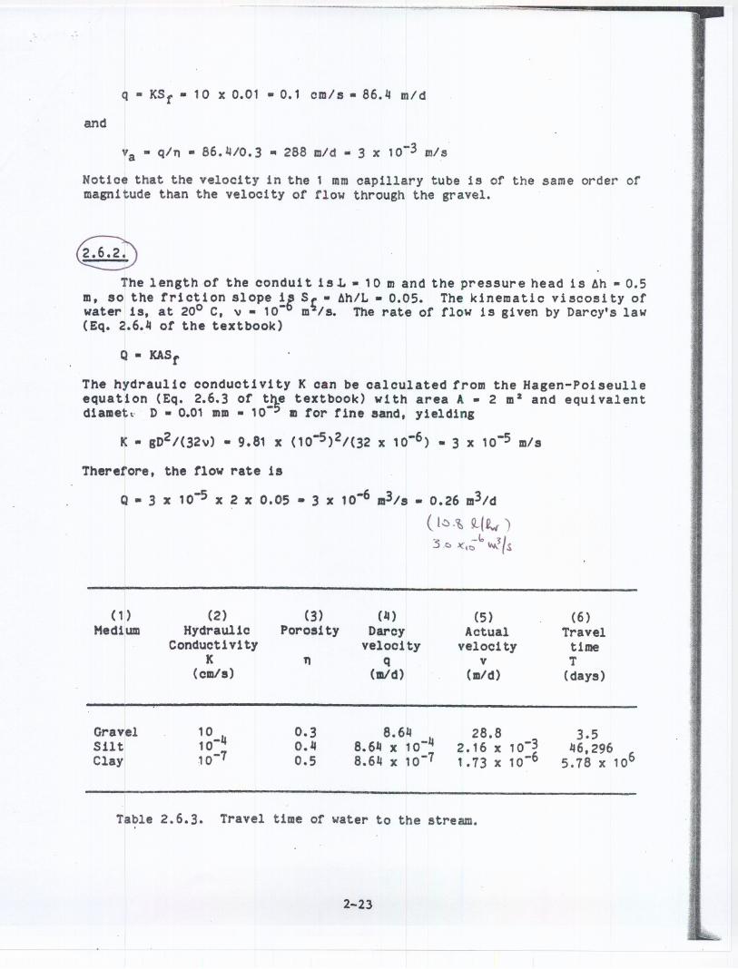
@The length of the condui t is.L ·10m and the pressure head is Ah ·0.5
m, so the friction slope ie S~·Ah/L ·0.05. The kinematic viscosi ty ofwater is, at 200 C, v · 10- m Is. The rate of flow is given by Darcy's law(Eq. 2.6.4 of the textbook)
Q · lCASf
The hydraulic conductivity K can be calculated from the Hagen-Poiseulle
equation (Eq. 2.6.3 of ~~e textbook) with area A . 2 m2 and equivalentdiamet~.D. 0.01mm· 10 mfor fine sand, yielding
K · gD2/(32v) · 9.81 x (10-5)2/(32 x 10-6) .3 x 10-5 m/s
Therefore, the flow rate is
Q ·3 x 10-5x 2 x 0.05 - 3 x 10⁻⁶m3/s- 0.26 m3/d
( t~.~ !l(fw)3 _to 1/.Co KIt) \lit,: oS
(1)Medium
(2)Hydraulic
ConductivityK
(cm/s)
(3)Porosity
(4)Darcy
velocityq
(mid)
(5)Actual
velocityv
(mId)
(6)Travel
timeT
(days)"
GravelSiltClay
3.546,296
5.78 x 10⁶
0.30.40.5
28.82.16 x 10-31.73 x 10⁻⁶
Table 2.6.3. Travel time of water to the stream.
2-23
..

~~~The saturated vapor pressure at T - 25 °c 1s given by Equation (3.2.9)
ot the textbook
es- 611 exp(17.~1T/(237.3+T)J - 611 exp[11.27 x 25/(237.3 + 25»)~ tI.~
so es -~ Pa. The actual vapor pressure, e, 1s calculated by the samemethod substituting the dew point temperature Td - 20 °c tor T
e . 611 exp(17.27Td/(237.3+Td») - 611 exp[17.27 x 20/(237.3 + 20»)Z-33<J
soe." Pa.The relative hum1d1ty, trom Equation (3.2.11) ot the textbook, 1s
L~~ / ~H.qRh· .e/es· ~/a5t8 · 0 0.14-
and the specific humidity is' liven by Equation (3.2.6) ot the texbook, withair pressure p. 101.1 X 10' Pa
"2.~~<i
qv.w 0.622 elp · 0.622 x 1:f8ff/(101.1 x 10') - o~ O_Ol#
The las oonstant tor air, Ra' is liven by Equation (3.2.8) ot the texbook+.
Ra w 287 (1 . 0.608 qv> · 287 (1 · 0.608 x 0.01~) - 289'J/(kl.~)
and the air density i8 oalculated trom the ideal ,as law (Equation 3.2.7 otthe textbook) with temperature T · 273 . 25 · 298 "K, so that
Pa · pI (RaT) · 101.1 x 10'/(289 x 298) · 1.17 kl/m' J
3.2.2.
The temperature TI at elevation %. . 1500 m is given by Equation(3.2.16) ot the textbook with Ta · 250C, za · 0, and lapse rate CI. 9 °C/km,so that.
T. . T. - a (za - z.> · 25 - 4)x 10-3 (1500- 0) . 11.5 °c . 2811.5oK
This temperature is below the dew point temperature tor surface conditions,Td · 20 °c, so the vapor pressure at 1500 m elevation corresponds to thesaturated vapor pressure given by Equation (3.2.9) ot the textbook
es · 611 exp[17.21T/(237.3+T») · 611 exp[17.27 x 11.5/(237.3 + 11.5»)
so e · es · 1357 Pa.
The air pressure P. at %. -1500 misgiven by Equation (3.2.15) tromthe textbook, with PI · 101.1 kPa, ~o that
Pa. P. (T,IT.)S/(oRd). 101.1x (28~.5/298)9.81/(0.009 x 289). 8~.9kPa
3-2.~..

Surface Temperature Precipitable Water
(rnm)
o102030110
9.9520.77111.01
77.03138.39
Table 3.2.6. Variation of prec1p1 tablewater depth with surface temperature.
From Equation (3.3.11) of the textbook, the terminal veloci ty vt of afalling raindrop of diameter D · 2 mm · 0.002 m, with Cd · 0.517 from Table3.3.1 of the textbook, is
vt ~ [lIgD/(3Cd) (pw/Pa - 1»)1/2
. (II x 9.81 x 0.002/(3 x 0.517) (998/1.20 - 1)J1/2 .6.118 m/s
this is the drop velocity relative to the surrounding air. If the air isris1ns with velocity va - - 5 mIs, the absolute velocity ot the drop is
vrel - Vt + va · 6.118 - 5 · 1.118 m/s
and the drop 1s falling.
For drop diameter D · 0.2 mm · 0.0002 m, wi th Cct . 11..2,the terminalvelocity can be calculated similarly, resulting Vt · 0.12 mls and
vrel · Vt + va · 0.12 - 5 · - 11.28m/s
and the drop is rising.
Three vertical forces act on a falling raindrop: a gravity force Fw dueto its weight, a buoyancy torce Fb due to the air displaced by the drop anda drag force Fd caused by the fr'ction between the drop and the surroundingair. If v 1s the vertical fal~ velocity of the drop of mass m, fromNewton's law
3-8
'.
'J.
I'
"
f.
I:
The maximum rainfall depth recorded in 10, 20 and 30 min. intervals isfound by computing the running totals in Cols. (J4),(5) and (6) of Table3~~.3, respectively, through the storm, then selecting the maximum value ofthe corresponding series, as shown in Table 3.4.3. For example, for a 30minute time interval, the maximum 30 minute depth is 1.16 in, recordedbetween 5 and 35 min. The rainfall intensity (depth divided by time)corresponding to this depth is 1.16 in/O.5 hr - 2.32 in/hr.' This value isless than 60 ~ of the 3Q min intensity' experienced at gage 1-Bee for thesame storm (see Table 3.4.1 from the textbook).
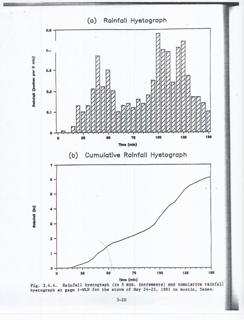
The computations follow those in Problem 3.J4.3.and are summarized inTable 3.~.4. The storm hyetograph is shown in Fig. 3.4.4(a). Thecumulative rainfall hyetograph, or rainfall mass curve, is obtained in Col.(3) of Table 3.4.~, and plot.ted in Fig. 3.4.4(b).
The maximum rainfall depth or intensity (depth divided by time)recorded in 10, 30, 60, 90 and 120 min. intervals is found by computing therunning totals in Cols. (4)-(8) of the table, through the storm, thenselecting the maximum v~ue of the corresponding series, as shown in Table3.4.4. These intensities are about 60-70 ~ of the intensities observed atgage 1-Bee for the same storm (see Table 3.4.1 from the textbook), whichexperiencedmore severe rainfall. .
3.11.5.
(a) Arithmetic mean method. Raingages numbers 1, 4, 6 and 8 arelocated outside the watershed and will not be considered in the computationot the arithmetic mean. The areal average rainfall is, therefore,
p. (Pa + PI + p. + P, + P,)/5
· (59 + 111 + 105 + 60 + 81)/5 · 69.2 mm
(b) Thiessen method. The Thiessen pOlygon network is shown in Fig.3.11.5-1. The areas assigned to each station are shown in Col. (3) of Table
3.4.5-1. The watershed area is A - 125 kma and the areal average rainfallis gi ven by Eq. (3.4.1) ot the textbook
J
P· 1/A I AjPj. 8746/125 · 70.0 mmj.1
(c) Isohyetal method. The isohyetal map is shown in Fig. 3.Jf.5-2.The average rainfall is found by adding the weighted .rainfall values in Col.(4) of Table 3.~.5-2,
J
p. 1/A r AjPj - 8638/125 · 69.1 mmJ-1
3-16

Time Rain (in) Cum Rain 10min 30min 60min 90in 120min0 0 0 0 0 0 0 05 0.09 0.09 0 0 0 0 0
10 0 0.09 0.09 0 0 0 015 0.03 0.12 0.03 0 0 0 020 0.13 0.25 0.16 0 0 0 025 0.1 0.35 0.23 0 0 0 030 0.13 0.48 0.23 0.48 0 0 035 0.21 0.69 0.34 0.6 0 0 040 0.37 1.06 0.58 0.97 0 0 045 0.22 1.28 0.59 1.16 0 0 050 0.3 1.58 0.52 1.33 0 0 055 0.2 1.78 0.5 1.43 0 0 060 0.1 1.88 0.3 1.4 1.88 0 065 0.13 2.01 0.23 1.32 1.92 0 070 0.14 2.15 0.27 1.09 2.06 0 075 0.12 2.27 0.26 0.99 2.15 0 080 0.16 2.43 0.28 0.85 2.18 0 085 0.14 2.57 0.3 0.79 2.22 0 090 0.18 2.75 0.32 0.87 2.27 2.75 095 0.25 3 0.43 0.99 2.31 2.91 0
100 0.48 3.48 0.73 1.33 2.42 3.39 0105 0.4 3.88 0.88 1.61 2.6 3.76 0110 0.39 4.27 0.79 1.84 2.69 4.02 0115 0.24 4.51 0.63 1.94 2.73 4.16 0120 0.41 4.92 0.65 2.17 3.04 4.44 4.92125 0.44 5.36 0.85 2.36 3.35 4.67 5.27130 0.27 5.63 0.71 2.15 3.48 4.57 5.54135 0.17 5.8 0.44 1.92 3.53 4.52 5.68140 0.17 5.97 0.34 1.7 3.54 4.39 5.72145 0.14 6.11 0.31 1.6 3.54 4.33 5.76150 0.1 6.21 0.24 1.29 3.46 4.33 5.73
Max Depth 0.48 0.88 2.36 3.54 4.67 5.76Intensity (in/hr) 5.76 5.28 4.72 3.54 3.11 2.88
(a) Rainfall Hyetograph"
,
o :&I 10' 71 100 '21 '10
"11IM ("'In)
Fig. 3.4.4. Rainfall hyetograph (in 5 min. increments) and cumulative rainfall Ihyetograph at gage l-WLN for the storm of Hay 24-25, 1981 in Austin, Texas.
D.I
o:18 100 ,. ,.. 71
1'IIMe-)
Cumulative Rainfall Hyetograph
--- --
0.-
i,E.
o.at
I 0.2-iI
0.1
1
..// i/.I
""" - '? /;I /
'7 ;I V;I ;I V;I I- ;I
ti;I
;I I /I II I -
.J """j 1..1
'""!- '""!
""'!
C'" , ., .,C'"I- ""'! ., ""!
rJ-. . . I . I