CE 134L ELEMENTARY SURVEYING LABORATORY LABORATORY …hturner/ce134/lab2v8.pdf · CE 134 Laboratory Notes, Spring 2003 CE 134L ELEMENTARY SURVEYING LABORATORY LABORATORY # 11 INTRODUCTION

CE 134 Laboratory Notes, Spring 2003

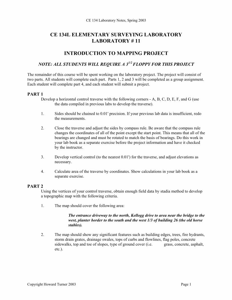
CE 134L ELEMENTARY SURVEYING LABORATORY LABORATORY # 11

INTRODUCTION TO MAPPING PROJECT

NOTE: ALL STUDENTS WILL REQUIRE A 31/2 FLOPPY FOR THIS PROJECT

The remainder of this course will be spent working on the laboratory project. The project will consist of two parts. All students will complete each part. Parts 1, 2 and 3 will be completed as a group assignment. Each student will complete part 4, and each student will submit a project. PART 1

Develop a horizontal control traverse with the following corners - A, B, C, D, E, F, and G (use the data compiled in previous labs to develop the traverse).

1. Sides should be chained to 0.01' precision. If your previous lab data is insufficient, redo

the measurements. 2. Close the traverse and adjust the sides by compass rule. Be aware that the compass rule

changes the coordinates of all of the point except the start point. This means that all of the bearings are changed and must be rotated to match the basis of bearings. Do this work in your lab book as a separate exercise before the project information and have it checked by the instructor.

3. Develop vertical control (to the nearest 0.01') for the traverse, and adjust elevations as

necessary. 4. Calculate area of the traverse by coordinates. Show calculations in your lab book as a

separate exercise. PART 2

Using the vertices of your control traverse, obtain enough field data by stadia method to develop a topographic map with the following criteria. 1. The map should cover the following area:

The entrance driveway to the north, Kellogg drive to area near the bridge to the west, planter border to the south and the west 1/3 of building 26 (the old horse stables).

2. The map should show any significant features such as building edges, trees, fire hydrants,

storm drain grates, drainage swales, tops of curbs and flowlines, flag poles, concrete sidewalks, top and toe of slopes, type of ground cover (i.e. grass, concrete, asphalt, etc.).

Copyright Howard Turner 2003 Page 1


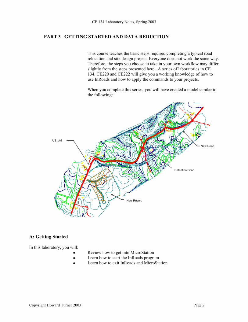
PART 3 –GETTING STARTED AND DATA REDUCTION

This course teaches the basic steps required completing a typical road relocation and site design project. Everyone does not work the same way. Therefore, the steps you choose to take in your own workflow may differ slightly from the steps presented here. A series of laboratories in CE 134, CE220 and CE222 will give you a working knowledge of how to use InRoads and how to apply the commands to your projects. When you complete this series, you will have created a model similar to

e following: th

US_old

New Resort

Retention Pond

New Road

A: Getting Started In this laboratory, you will: Review how to get into MicroStation Learn how to start the InRoads program Learn how to exit InRoads and MicroStation



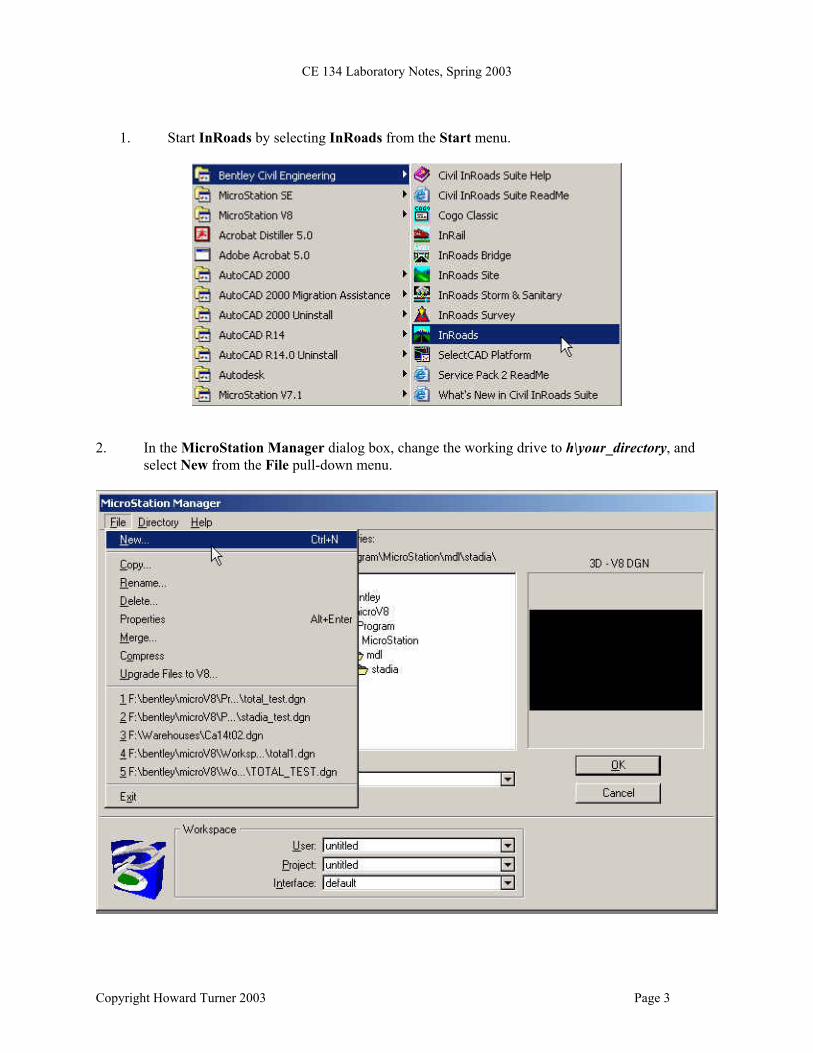
1. Start InRoads by selecting InRoads from the Start menu.

2. In the MicroStation Manager dialog box, change the working drive to h\your_directory, and

select New from the File pull-down menu.



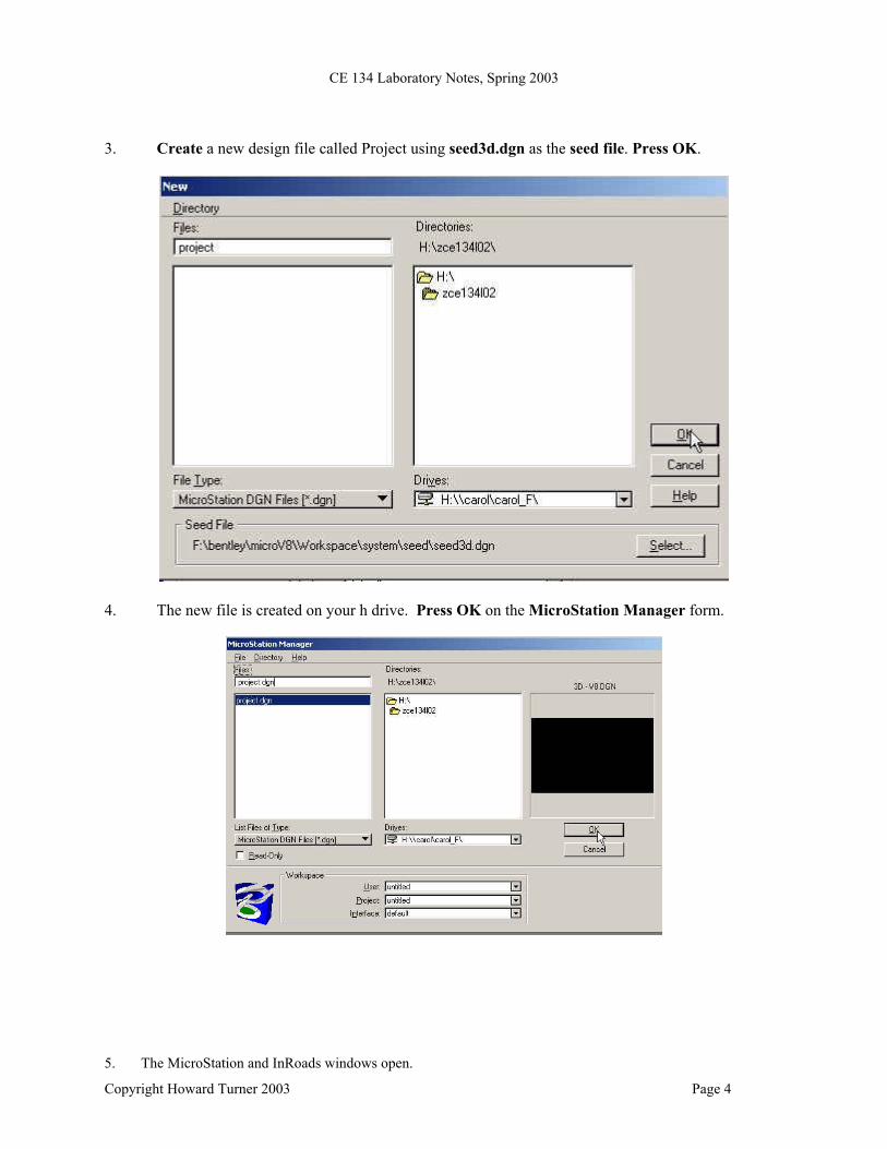
3. Create a new design file called Project using seed3d.dgn as the seed file. Press OK.

4. The new file is created on your h drive. Press OK on the MicroStation Manager form.

5. The MicroStation and InRoads windows open.



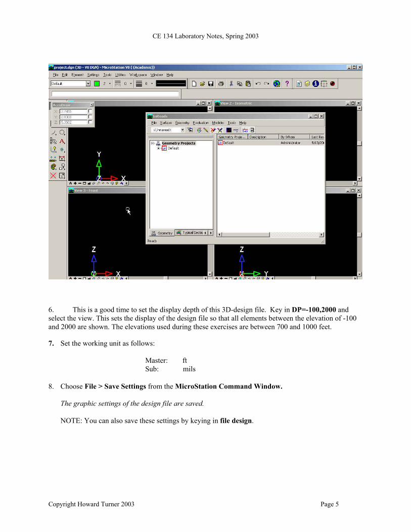
6. This is a good time to set the display depth of this 3D-design file. Key in DP=-100,2000 and select the view. This sets the display of the design file so that all elements between the elevation of -100 and 2000 are shown. The elevations used during these exercises are between 700 and 1000 feet. 7. Set the working unit as follows: Master: ft Sub: mils 8. Choose File > Save Settings from the MicroStation Command Window. The graphic settings of the design file are saved. NOTE: You can also save these settings by keying in file design.



B -Data Reduction 1. Use the BASIC traverse program supplied by the instructor to adjust the polygon by compass

rule. Keep a copy of the printout; you will need the results in the next step. This program requires line direction in azimuth. The reference azimuth is line BC. The azimuth of line BC is 181o 47’ 27”.

2. Open notepad (You will find notepad under “Programs -> Accessories -> Notepad”). Notepad will be used to create a file called “Control”. This file must be saved in your own directory. You may give the file any name. 3. Enter your control data (obtained by adjusting the traverse data) in the file in the following

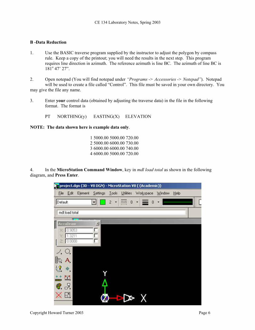
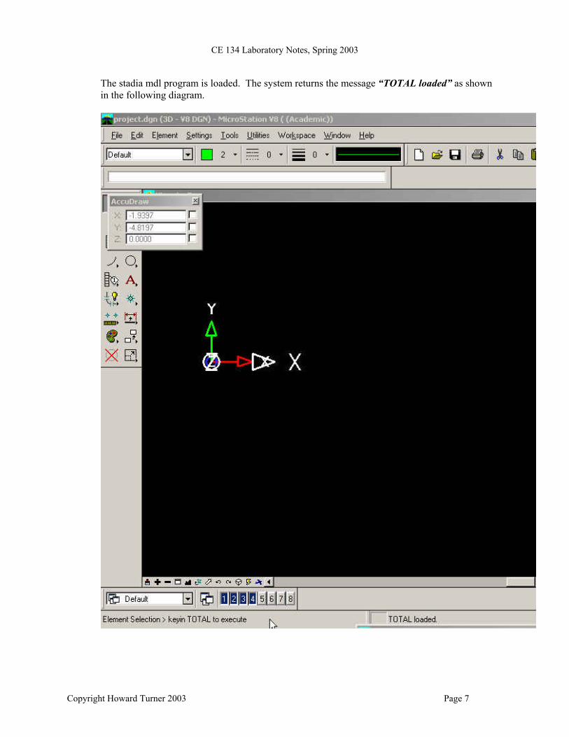
format. The format is PT NORTHING(y) EASTING(X) ELEVATION NOTE: The data shown here is example data only. 1 5000.00 5000.00 720.00 2 5000.00 6000.00 730.00 3 6000.00 6000.00 740.00 4 6000.00 5000.00 720.00 4. In the MicroStation Command Window, key in mdl load total as shown in the following diagram, and Press Enter.



The stadia mdl program is loaded. The system returns the message “TOTAL loaded” as shown in the following diagram.



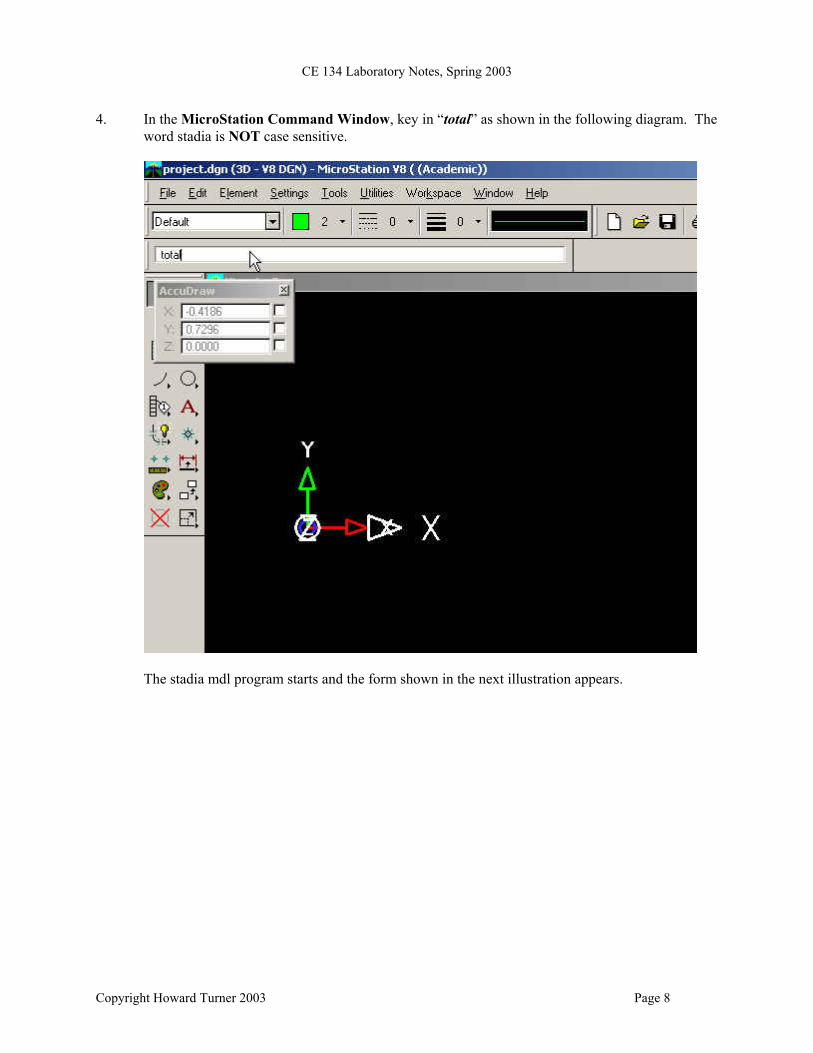
4. In the MicroStation Command Window, key in “total” as shown in the following diagram. The word stadia is NOT case sensitive.

The stadia mdl program starts and the form shown in the next illustration appears.



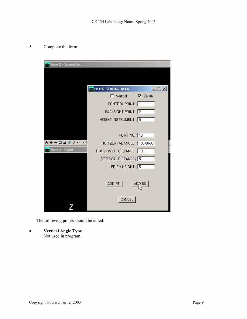
5. Complete the form.

The following points should be noted:

a. Vertical Angle Type Not used in program.



b. Control Point The occupied point at the time the measurement is made. The point number is entered. The coordinates of the control point are obtained from the control file. The control point must be an integer value (e.g. 4).

c. Backsight Point

The backsight point at the time the measurement is made. The point number is entered. The coordinates of the backsight point are obtained from the control file. The backsight point must be an integer value (e.g. 5).

d. Height of Instrument

The height of the telescope axis above the ground on the instrument set on the control point. The value should be given as a real number to two decimal places (e.g. 5.34). If the prism height was set to the same height as the instrument, any value can be used, as long as it is the same value as the prism height.

e. Point Number

The point number assigned to the new elevation point. The point number must be an integer value (e.g. 20).

f. Horizontal Angle The angle observed to the new elevation point. An angle measured to the right with a value >=0o and < 360o. Hyphens must separate the degrees, minutes and seconds. This is the only separator allowed (e.g. 45-00-00).

g. Horizontal Distance The horizontal distance observed to the new elevation point. .

h. Vertical Distance The vertical distance observed to the new elevation point. .

i. Prism Height

The height of the center of the prism above the ground. The value should be given as a real number to two decimal places (e.g. 5.34). If the prism height was set to the same height as the instrument, any value can be used, as long as it is the same value as the instrument height.



6. Press the button NEW BS with the mouse cursor. The system responds with the message “new

backsight button pressed”. A new setup for a control point is processed. A light blue dot of weight 5 will appear at the location of the control point in the MicroStation file. A red dot of weight 3 will appear for the location of the new elevation point. The point number is written against the dot in purple.

7. Complete the stadia form from point number onwards for all remaining point obtained from the

same control point. Press the NEW PT button with the mouse cursor. The system responds with “new pt button pressed”. A red dot of weight 3 will appear for the location of the new elevation point. The point number is written against the dot in purple.

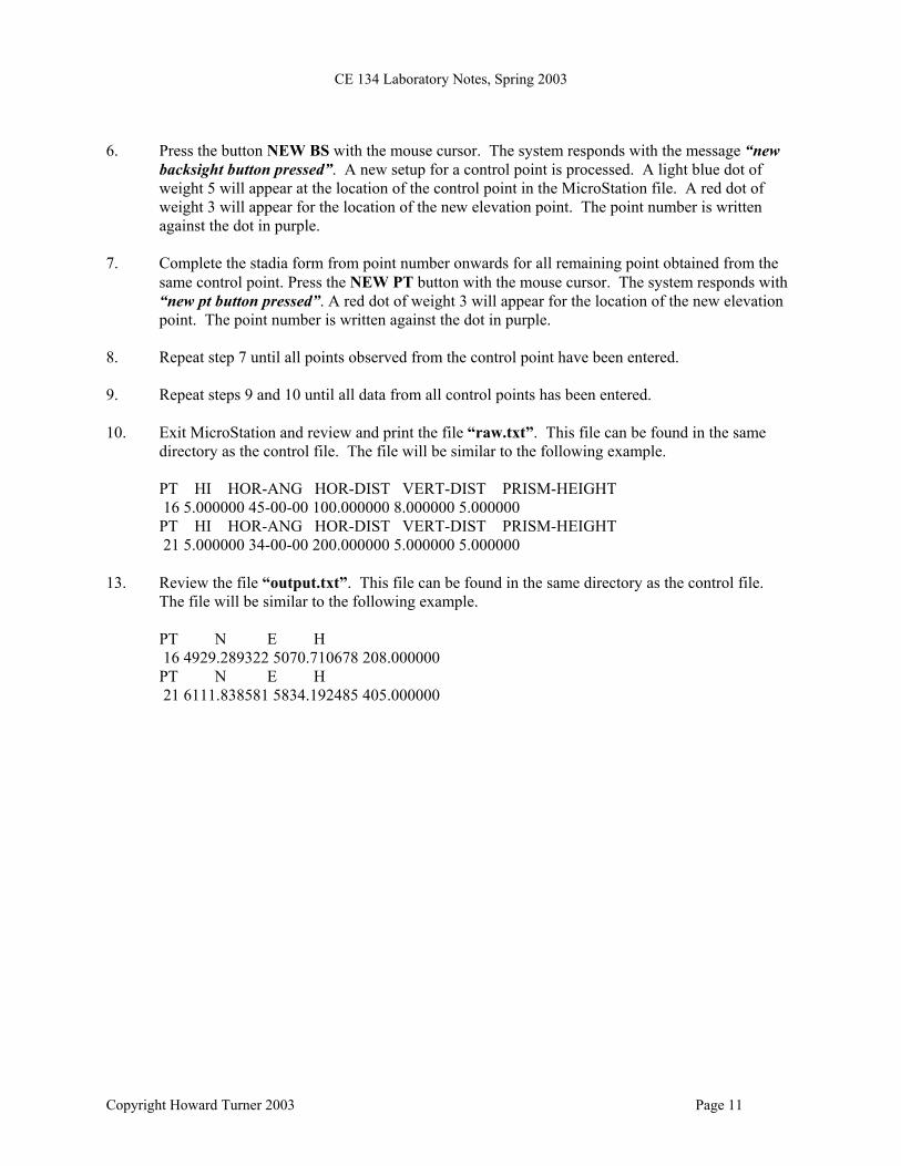
8. Repeat step 7 until all points observed from the control point have been entered. 9. Repeat steps 9 and 10 until all data from all control points has been entered. 10. Exit MicroStation and review and print the file “raw.txt”. This file can be found in the same

directory as the control file. The file will be similar to the following example.

PT HI HOR-ANG HOR-DIST VERT-DIST PRISM-HEIGHT 16 5.000000 45-00-00 100.000000 8.000000 5.000000 PT HI HOR-ANG HOR-DIST VERT-DIST PRISM-HEIGHT 21 5.000000 34-00-00 200.000000 5.000000 5.000000

13. Review the file “output.txt”. This file can be found in the same directory as the control file. The file will be similar to the following example.

PT N E H 16 4929.289322 5070.710678 208.000000 PT N E H 21 6111.838581 5834.192485 405.000000



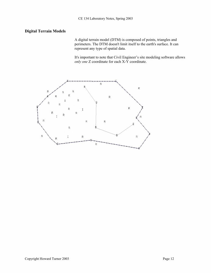
Digital Terrain Models A digital terrain model (DTM) is composed of points, triangles and perimeters. The DTM doesn't limit itself to the earth's surface. It can represent any type of spatial data. It's important to note that Civil Engineer’s site modeling software allows only one Z coordinate for each X-Y coordinate.



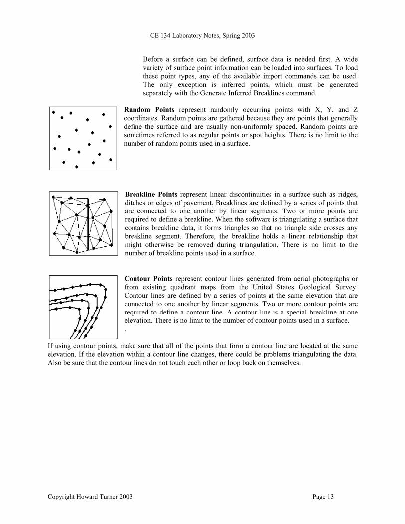
Before a surface can be defined, surface data is needed first. A wide variety of surface point information can be loaded into surfaces. To load these point types, any of the available import commands can be used. The only exception is inferred points, which must be generated separately with the Generate Inferred Breaklines command.

Random Points represent randomly occurring points with X, Y, and Z coordinates. Random points are gathered because they are points that generally define the surface and are usually non-uniformly spaced. Random points are sometimes referred to as regular points or spot heights. There is no limit to the number of random points used in a surface.

Breakline Points represent linear discontinuities in a surface such as ridges, ditches or edges of pavement. Breaklines are defined by a series of points that are connected to one another by linear segments. Two or more points are required to define a breakline. When the software is triangulating a surface that contains breakline data, it forms triangles so that no triangle side crosses any breakline segment. Therefore, the breakline holds a linear relationship that might otherwise be removed during triangulation. There is no limit to the number of breakline points used in a surface. Contour Points represent contour lines generated from aerial photographs or from existing quadrant maps from the United States Geological Survey. Contour lines are defined by a series of points at the same elevation that are connected to one another by linear segments. Two or more contour points are required to define a contour line. A contour line is a special breakline at one elevation. There is no limit to the number of contour points used in a surface. .

If using contour points, make sure that all of the points that form a contour line are located at the same elevation. If the elevation within a contour line changes, there could be problems triangulating the data. Also be sure that the contour lines do not touch each other or loop back on themselves.



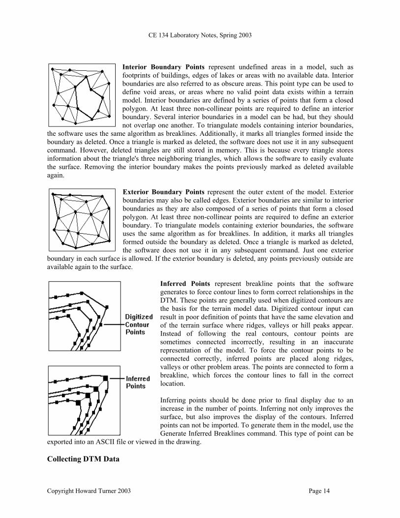
Interior Boundary Points represent undefined areas in a model, such as footprints of buildings, edges of lakes or areas with no available data. Interior boundaries are also referred to as obscure areas. This point type can be used to define void areas, or areas where no valid point data exists within a terrain model. Interior boundaries are defined by a series of points that form a closed polygon. At least three non-collinear points are required to define an interior boundary. Several interior boundaries in a model can be had, but they should not overlap one another. To triangulate models containing interior boundaries,

the software uses the same algorithm as breaklines. Additionally, it marks all triangles formed inside the boundary as deleted. Once a triangle is marked as deleted, the software does not use it in any subsequent command. However, deleted triangles are still stored in memory. This is because every triangle stores information about the triangle's three neighboring triangles, which allows the software to easily evaluate the surface. Removing the interior boundary makes the points previously marked as deleted available again.

Exterior Boundary Points represent the outer extent of the model. Exterior boundaries may also be called edges. Exterior boundaries are similar to interior boundaries as they are also composed of a series of points that form a closed polygon. At least three non-collinear points are required to define an exterior boundary. To triangulate models containing exterior boundaries, the software uses the same algorithm as for breaklines. In addition, it marks all triangles formed outside the boundary as deleted. Once a triangle is marked as deleted, the software does not use it in any subsequent command. Just one exterior

boundary in each surface is allowed. If the exterior boundary is deleted, any points previously outside are available again to the surface.

Inferred Points represent breakline points that the software generates to force contour lines to form correct relationships in the DTM. These points are generally used when digitized contours are the basis for the terrain model data. Digitized contour input can result in poor definition of points that have the same elevation and of the terrain surface where ridges, valleys or hill peaks appear. Instead of following the real contours, contour points are sometimes connected incorrectly, resulting in an inaccurate representation of the model. To force the contour points to be connected correctly, inferred points are placed along ridges, valleys or other problem areas. The points are connected to form a breakline, which forces the contour lines to fall in the correct location. Inferring points should be done prior to final display due to an increase in the number of points. Inferring not only improves the surface, but also improves the display of the contours. Inferred points can not be imported. To generate them in the model, use the Generate Inferred Breaklines command. This type of point can be

exported into an ASCII file or viewed in the drawing.

Collecting DTM Data



Several rules must be kept in mind while collecting surface data. Accurate data collection is essential for producing accurate models. First, the correct spacing of random points and the correct placement of breaklines are critical to accurately modeling physical sites. Random points should be colleted at all local minima and maxima within a site. A local minimum or maximum is a location within the modeled site that is at a low or high elevation relative to neighboring points. Additionally, random points should be collected throughout the site so that the distance from one random point to another is about equal. Breakline data should be added to force the model to accurately represent areas where there are discontinuities in the terrain surface. Such features include the top and bottom of ditches and the edges of roadway pavement. Additionally, in certain circumstances where modeling areas include ridge or valley lines, breaklines that follow these features will want to be added. In general, breaklines should not cross one another, although the software allows this condition. If breaklines cross, problems may be experienced when triangulating the surface. Crossing breaklines should have the same elevation at their intersection since a surface cannot contain two points at the same X, Y and have a different Z.

Field Survey Data

When collecting terrain model data through field surveys, survey crews typically collect random points in a regular, grid-like fashion. Although the distances between these points varies from site to site, it normally ranges from 5 to 50 meters, depending on the topography. To fine-tune the accuracy of the model, topographic measurements along lines where there is an obvious break in the terrain slope are also collected. This second set of points is added as breaklines. Finally, if there are certain areas on the site that need to be excluded from the model, such as the footprints of large buildings, the survey crew collects data points defining the perimeter of the area and adds these to the model as interior boundary points.

Photogrammetric or Digitized Data

If surface data is collected with photogrammetric or digitized data, two different techniques to input the data may be used. The first method is very similar to that used by field survey crews. Collect random points in a fairly equal-spaced, grid-like pattern, and then supplement them with more detailed breakline and interior boundary data. This method takes a little more time, but is more accurate. The second technique generally results in less accurate models. It digitizes existing contour information directly and uses that information as the basis for the terrain model. It is best not to stream digitize contours because it creates too many unnecessary points in your model. Even so, this very dense data can still be managed with the InRoads family of products.

When using photogrammetric or digitized data, different point types should be separated on different drawing file levels. For example, place



random points on level 11 and contour points on level 12. This makes it easier to work with the model. No matter how the data is collected, remember to collect the right amount of information. Too little information causes a coarse, inaccurate model. Too much information can slow processing.

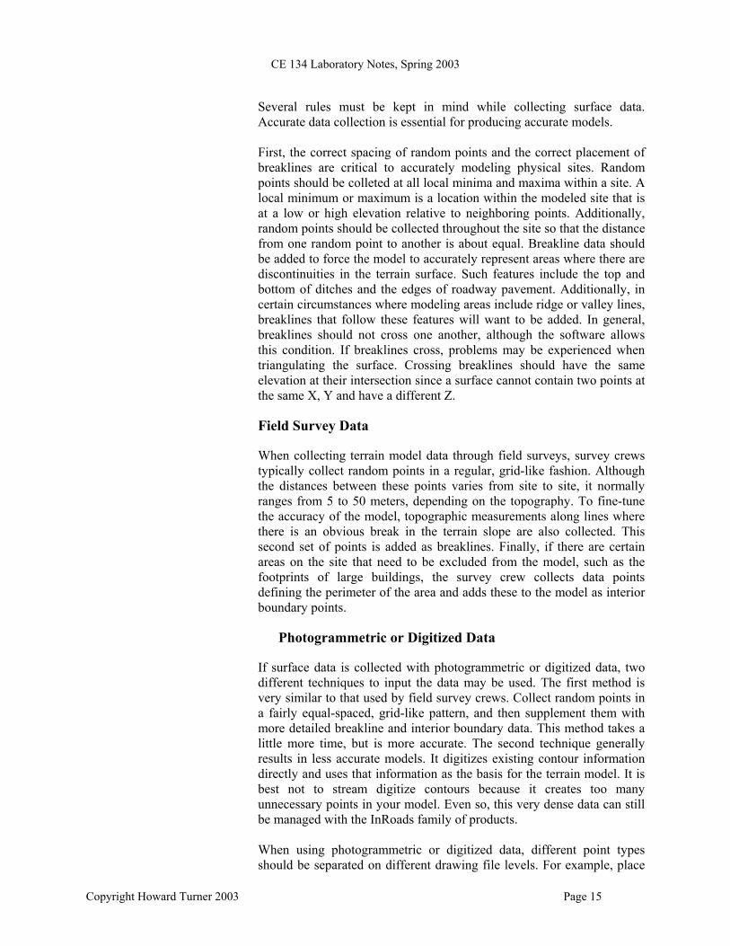
After the Data is Loaded After the point data is loaded to the surface, the software is used to triangulate the data, associating the points and defining the surface by drawing lines between the points.

Select which surface to triangulate and the maximum triangle length. For example, a zero length indicates infinity. After the surface is triangulated, save it. Define the location and the name of the surface file. After saving the surface, it can be reloaded or opened later. For more information about saving, naming, and opening existing surfaces, refer to the Help files. Next, review the surface to see the minimum and maximum coordinate range. Reviewing the surface shows whether any points are out of range. After reviewing the surface, the software can be used to edit it. The Help files have more information about the surface editing commands. Display surface information such as contours and triangles and color-code the elevation ranges. When using contours, the command to establish the parameter settings for the display is selected, such as contour spacing and the number of minor contours between each major contour.



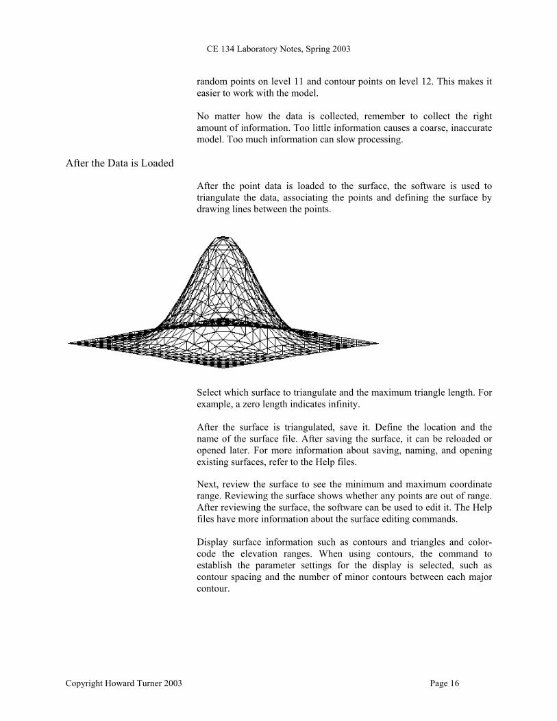
If Write Lock is off when contours are displayed, the graphics will disappear when the view is updated. If Write Lock is on when the contours are displayed, the contours display permanently. There are many ways to add, change, and store surface information. The on-line Help files include many additional details.

What Is a Feature? What is a Feature? A feature is a unique instance of a 3D surface item or entity in a DTM. A feature can be one of five types, corresponding to the different types of DTM points: random, breakline, exterior boundary, interior boundary or contour. Although features are a new and powerful concept, they are essentially one or more items contained in a digital terrain model. Any one item or group is given a name and assigned a feature style. Feature Styles controls everything about how a feature gets displayed. The ability to identify different features by name, to select and edit them using filters, and to independently control their display characteristics are benefits of organizing the DTM into features.

Random Features versus Breakline Features



The purpose of this section is to explain some key differences between random features and breakline features. Remember that all features, regardless of type (breakline, random, interior, …) are basically defined as a 3D entity. Features are groups (or single), points or elements. This discussion attempts to explain the significance between the two most common types: breakline features and random features.

Breakline Features Breakline features represent groups of DTM points with an important linear relationship. A few examples of breaklines are the edge of a roadway lane, the bottom of a ditch, the edge of a curb, and so on. When a DTM is triangulated, breakline features are honored in such a way that no triangle edge (triangle leg) will cross the path defined by connecting the points in the breakline feature. Breaklines, thus, promote accuracy in the triangulated model. The breakline designation implies significance to the linear path between each point in the feature. As a result, breakline features can appear in cross sections, whereas random features cannot. This is a critical difference. Also, with the software, a point density interval can be applied to your breakline features, ensuring that numerous triangle vertices will appear along each feature leg. However, the point density interval cannot be applied to random features.

Random Features Random features represent distinct points with no significant linear relationship. Random points typically represent general terrain elevations. Because there is no important linear relationship among the points in the random feature, random features cannot be displayed in cross sections. A point density interval cannot be applied to a random feature. Displaying Linear versus Point Data With the software, the points that define a feature can be displayed, as well as the connecting line segments between those points. This is true for all feature types-- even random features. In fact, the connecting line segments and not the actual 3D feature points can be chosen to be displayed. The settings that control what gets displayed are in the feature style. On the other hand, just the points from a breakline feature can be chosen to be displayed, even though the linear relationship is what is very important about these points. The key point to remember is the control one has on how features are displayed (points, line segments or both) regardless of the feature type.

Symbology for Displaying Features All of the display characteristics of features are controlled by feature styles. For more information on feature styles, see the Help topic on the



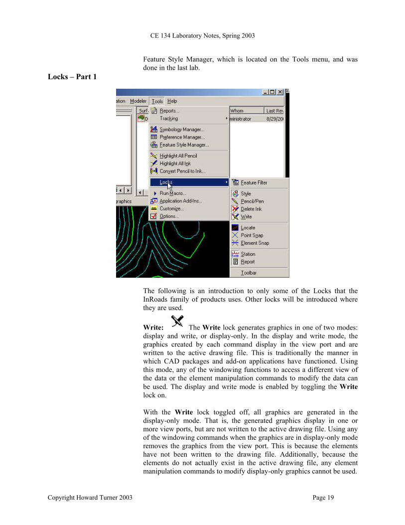
Feature Style Manager, which is located on the Tools menu, and was done in the last lab.

Locks – Part 1

The following is an introduction to only some of the Locks that the InRoads family of products uses. Other locks will be introduced where they are used.

Write: The Write lock generates graphics in one of two modes: display and write, or display-only. In the display and write mode, the graphics created by each command display in the view port and are written to the active drawing file. This is traditionally the manner in which CAD packages and add-on applications have functioned. Using this mode, any of the windowing functions to access a different view of the data or the element manipulation commands to modify the data can be used. The display and write mode is enabled by toggling the Write lock on. With the Write lock toggled off, all graphics are generated in the display-only mode. That is, the generated graphics display in one or more view ports, but are not written to the active drawing file. Using any of the windowing commands when the graphics are in display-only mode removes the graphics from the view port. This is because the elements have not been written to the drawing file. Additionally, because the elements do not actually exist in the active drawing file, any element manipulation commands to modify display-only graphics cannot be used.



Suppose there is a line placed in the drawing file. If the [Redraw] or View Update command were selected with the Write lock toggled on, the line redisplays in the drawing file. If the Write lock is toggled off and the command is selected, the line is removed from the screen. The display-only mode is extremely useful when needing to view large amounts of terrain model data and then quickly removing that data from the screen. Since the display-only mode does not write graphics to the active drawing file, it can decrease drawing file size and increase the speed in which all graphics display in views by using this mode. The Write lock can be enabled or disabled at any time, even when about to click the Apply button in one of the View commands.

Pencil/Pen: Pencil Pen Note: The Pencil/Pen lock is applicable only when the Write lock is on. Also, the Pencil/Pen lock applies to 3D display-only. It does not apply to cross sections or profiles. This command toggles the Pencil/Pen lock between Pencil mode and Pen mode. This lock affects the display of virtually every piece of 3D graphics representing surfaces or geometry. The Pencil/Pen lock controls what happens when a piece of graphics is redisplayed. Two actions may occur: one, the new graphics will display in addition to the old ones (Pen mode) or two, the new graphics will replace the old ones (Pencil mode). To keep previous work displayed and not lose it when modifying and redisplaying the surface or geometry, the Pen mode would be used. Pencil mode, on the other hand, is a convenience because it automatically cleans up the graphics from the previous work as it is modified in the design and redisplayed. The following two points summarize the basic notion of each mode: • Pen mode graphics are permanent and allow duplicates (see the

Delete Ink lock). • Pencil mode graphics persist only until an item is redisplayed; there

are no duplicates.

The effect of the Delete Ink Lock: Although the previous explanation refers to graphics drawn in Pen mode as “permanent,” this is not completely accurate. The graphics are permanent as far as Pen mode is concerned. However, if the Delete Ink lock is on at the time of redisplay, even graphics previously drawn in “ink” will be replaced by the new instance of the graphics. Please note that graphics drawn using Pen mode are said to be drawn in ink. The Delete Ink lock allows redisplayed graphics to replace even graphics that were drawn in ink. For example, a use for this might occur



if work were done in Pen mode for a while comparing different designs and before finally settling on a design (assume we are talking about an alignment). If the alignment were displayed several times in ink, the Delete Ink lock can be turned on and the alignment can be displayed one more time. All the previous instances of the alignment will be removed when the alignment is redisplayed. The Delete Ink lock will probably remain off most of the time. One Thing To Remember: It is critical to understand that the current setting of the Pencil/Pen lock is irrelevant in determining what will happen when a piece of graphics is redisplayed. What is relevant is whether the existing graphics are displayed in Pencil mode or in Pen mode. Style: The main concept behind the Style lock is data-driven symbology. The Style locks affects two groups of commands: · all the View Surface commands, and · the Annotate Cross Section command. Style Lock and the View Surface Commands The effect of the Style lock is this: When the Style lock is on and you activate a View Surface command, the dialog box for the command will not be displayed, but rather your surface data will be displayed in the graphics file without any further input from you. The Style lock bypasses the dialog box and displays the active surface, automatically determining what symbology to use. How is the symbology determined? When you run a View Surface command with Style lock on, the symbology is chosen according to the following procedure: 1) If a preference is associated with the active surface (see Surface Properties), the software reads this preference name and looks for a saved preference with a matching name in the command that you are running. If the command contains a saved preference by the same name as the preference that is specified in the active surface, then the issue of symbology is settled – the command is executed using that saved preference. 2) If there is no preference associated with the active surface or if there is no saved preference with a matching name, the software looks to the Preferred Preference. The Preferred Preference is defined under Tools > Options, on the General tab when the Category is set to Settings. If the View Surface command contains a saved preference by the same name as the Preferred Preference, the command is executed using that saved preference.


3) Finally, if the preference is still unresolved, the software just uses the Default preference. Every command has a Default preference – Default cannot be deleted.


When the Style lock is off, activating the View Surface command displays a dialog box, as usual, and the settings on the dialog box are used to control symbology. Style Lock and the Annotate Cross Section Command The effect of the Style lock on Cross Section commands is limited to only one command: Annotate Cross Section. Before considering exactly what the Style lock does for this command, you should understand that, in addition to specifying a preference name (see the previous discussion), a surface specifies a named symbology. To verify this, look at the Symbology field in the Cross Sections group box on the Advanced tab of the Surface Properties dialog box. The named symbology specified in this field is defined expressly for using the Style lock with the Annotate Cross Section command. Note For more information on named symbology, see the help topic on the Symbology Manager command. In the Create Cross Section command, the Style lock affects the symbology for the surface data line and for features, which are displayed as points in cross section. The other graphics displayed by this command (the title, legend, axes, and grid) are not affected by the Style lock. The symbology for these other pieces of graphics is controlled by the dialog box settings, which are stored in the preference file (CIVIL.INI). In the Annotate Cross Section command, the Style lock affects the symbology of point and segment annotation as well as feature annotation. Other graphics, such as the frame, ticks, and titles, are not affected by the Style lock. The symbology for these other pieces of graphics is controlled by the dialog box settings, which are stored in the preference file (CIVIL.INI). When the Style lock is on, the symbology for the point and segment annotation comes from the named symbology associated with the surface by the Symbology parameter on the Surface Properties dialog box. When the Style lock is off, the symbology comes from the feature style associated with each feature. Because each feature can have a unique feature style, it is possible for the annotation for each feature to be displayed with different symbology. Note Style Lock does not affect the profile commands. Locate: The Locate lock determines whether to snap to graphics displayed in the graphics file or to snap to the position occupied by a feature in the active surface. If the lock is set to graphics (the icon shows a single, red line), locate actions will seek the nearest displayed graphics. If the lock is set to features (the icon shows an image of a surface), locate actions will seek the position of the nearest feature in the active surface whether or not the feature is actually displayed. You can use the locate



lock to locate features that are not even displayed. If they exist in the DTM, the locate will find them Point Snap: When turned on, this lock enables the cursor to snap or lock onto the closest point defined in the geometry project. Element: When turned on, this lock enables the cursor to snap or lock onto the closest geometry element in the active geometry project. This can be used to extract distances and directions from that element to design new elements or points. Point Snap Lock and Element Lock cannot be turned on at the same time. Station: This lock is applicable only when the first station specified on the horizontal alignment is an odd-numbered station (for example, 2+39) and you are generating cross sections, executing the Roadway Modeler, or generating station-type reports. When this lock is turned on, the software applies a given command action to the first station, and forces all subsequent actions to even-numbered stations. For example, if the first station is 2+39, and the station interval is defined as 50, the software performs the command action at stations 2+39, 2+50, 3+00. and so on. When Station Lock is turned off and the first station is odd-numbered, the software applies the command action to odd-numbered stations only (for example 2+39, 2+89, 3+39).

Report: The Report lock is used by several commands to control whether or not the command displays output in a dialog box as the command calculations are performed. If this lock is off, the command processes and stores results without displaying them in an output dialog box.



SURFACE CREATION

NOTE: From this point on, unless stated differently, all commands will be chosen from the

InRoads menu.

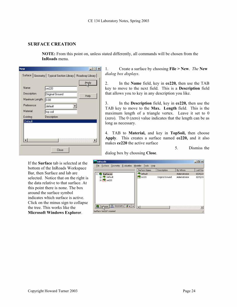
1. Create a surface by choosing File > New. The New dialog box displays. 2. In the Name field, key in ce220, then use the TAB key to move to the next field. This is a Description field that allows you to key in any description you like. 3. In the Description field, key in ce220, then use the TAB key to move to the Max. Length field. This is the maximum length of a triangle vertex. Leave it set to 0 (zero). The 0 (zero) value indicates that the length can be as long as necessary. 4. TAB to Material, and key in TopSoil, then choose Apply. This creates a surface named ce220, and it also makes ce220 the active surface 5. Dismiss the dialog box by choosing Close.

If the Surface tab is selected at the bottom of the InRoads Workspace Bar, then Surface and lab are selected. Notice that on the right is the data relative to that surface. At this point there is none. The box around the surface symbol indicates which surface is active. Click on the minus sign to collapse the tree. This works like the Microsoft Windows Explorer.



Loading Graphic Data in to a Surface

Now that the surface has been created, data can be entered into the surface.

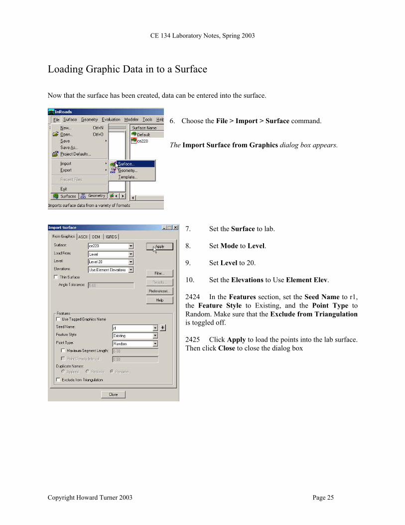
6. Choose the File > Import > Surface command. The Import Surface from Graphics dialog box appears.

7. Set the Surface to lab. 8. Set Mode to Level. 9. Set Level to 20. 10. Set the Elevations to Use Element Elev. 2424 In the Features section, set the Seed Name to r1, the Feature Style to Existing, and the Point Type to Random. Make sure that the Exclude from Triangulation is toggled off. 2425 Click Apply to load the points into the lab surface. Then click Close to close the dialog box



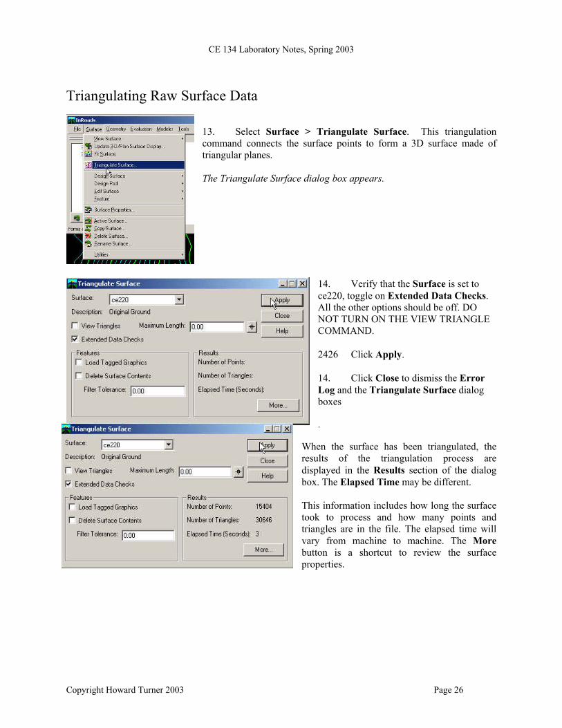
Triangulating Raw Surface Data 13. Select Surface > Triangulate Surface. This triangulation command connects the surface points to form a 3D surface made of triangular planes. The Triangulate Surface dialog box appears.

14. Verify that the Surface is set to ce220, toggle on Extended Data Checks. All the other options should be off. DO NOT TURN ON THE VIEW TRIANGLE COMMAND. 2426 Click Apply. 14. Click Close to dismiss the Error Log and the Triangulate Surface dialog boxes .

When the surface has been triangulated, the results of the triangulation process are displayed in the Results section of the dialog box. The Elapsed Time may be different. This information includes how long the surface took to process and how many points and triangles are in the file. The elapsed time will vary from machine to machine. The More button is a shortcut to review the surface properties.



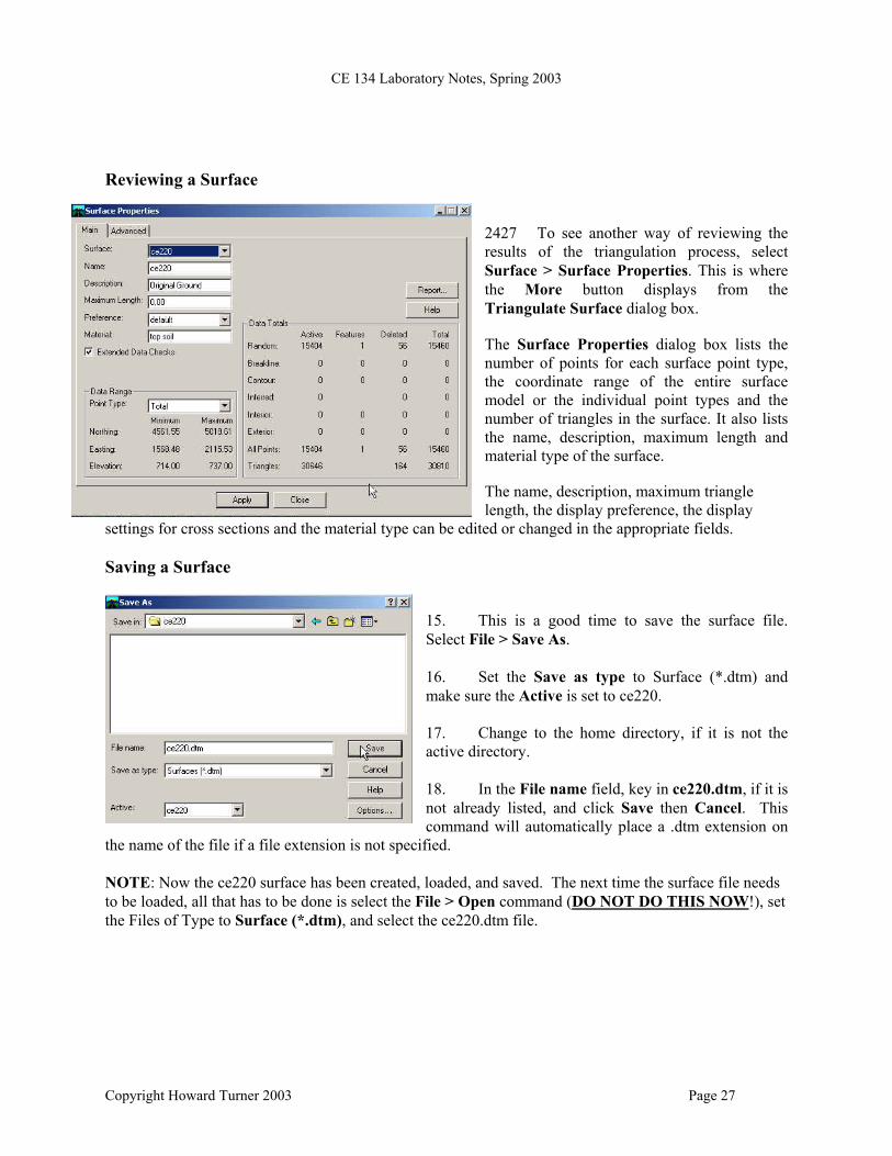
Reviewing a Surface 2427 To see another way of reviewing the results of the triangulation process, select Surface > Surface Properties. This is where the More button displays from the Triangulate Surface dialog box. The Surface Properties dialog box lists the number of points for each surface point type, the coordinate range of the entire surface model or the individual point types and the number of triangles in the surface. It also lists the name, description, maximum length and material type of the surface. The name, description, maximum triangle length, the display preference, the display

settings for cross sections and the material type can be edited or changed in the appropriate fields. Saving a Surface

15. This is a good time to save the surface file. Select File > Save As. 16. Set the Save as type to Surface (*.dtm) and make sure the Active is set to ce220. 17. Change to the home directory, if it is not the active directory. 18. In the File name field, key in ce220.dtm, if it is not already listed, and click Save then Cancel. This command will automatically place a .dtm extension on

the name of the file if a file extension is not specified.

NOTE: Now the ce220 surface has been created, loaded, and saved. The next time the surface file needs to be loaded, all that has to be done is select the File > Open command (DO NOT DO THIS NOW!), set the Files of Type to Surface (*.dtm), and select the ce220.dtm file.



Set up to Display Contours

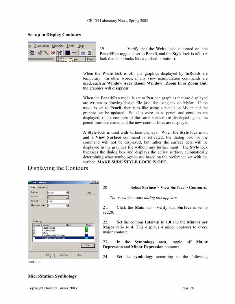
19 Verify that the Write lock is turned on, the Pencil/Pen toggle is set to Pencil, and the Style lock is off. (A lock that is on looks like a pushed in button).

When the Write lock is off, any graphics displayed by InRoads are temporary. In other words, if any view manipulation commands are used, such as Window Area [Zoom Window], Zoom In or Zoom Out, the graphics will disappear. When the Pencil/Pen mode is set to Pen, the graphics that are displayed are written to drawing/design file just like using ink on Mylar. If the mode is set to Pencil, then it is like using a pencil on Mylar and the graphic can be updated. So, if it were set to pencil and contours are displayed, if the contours of the same surface are displayed again, the pencil lines are erased and the new contour lines are displayed. A Style lock is used with surface displays. When the Style lock is on and a View Surface command is activated, the dialog box for the command will not be displayed, but rather the surface data will be displayed in the graphics file without any further input. The Style lock bypasses the dialog box and displays the active surface, automatically determining what symbology to use based on the preference set with the surface. MAKE SURE STYLE LOCK IS OFF.

Displaying the Contours

20 Select Surface > View Surface > Contours. The View Contours dialog box appears. 21. Click the Main tab. Verify that Surface is set to ce220. 22. Set the contour Interval to 1.0 and the Minors per Major ratio to 4. This displays 4 minor contours to every major contour. 23. In the Symbology area, toggle off Major Depression and Minor Depression contours. 24. Set the symbology according to the following

section. MicroStation Symbology



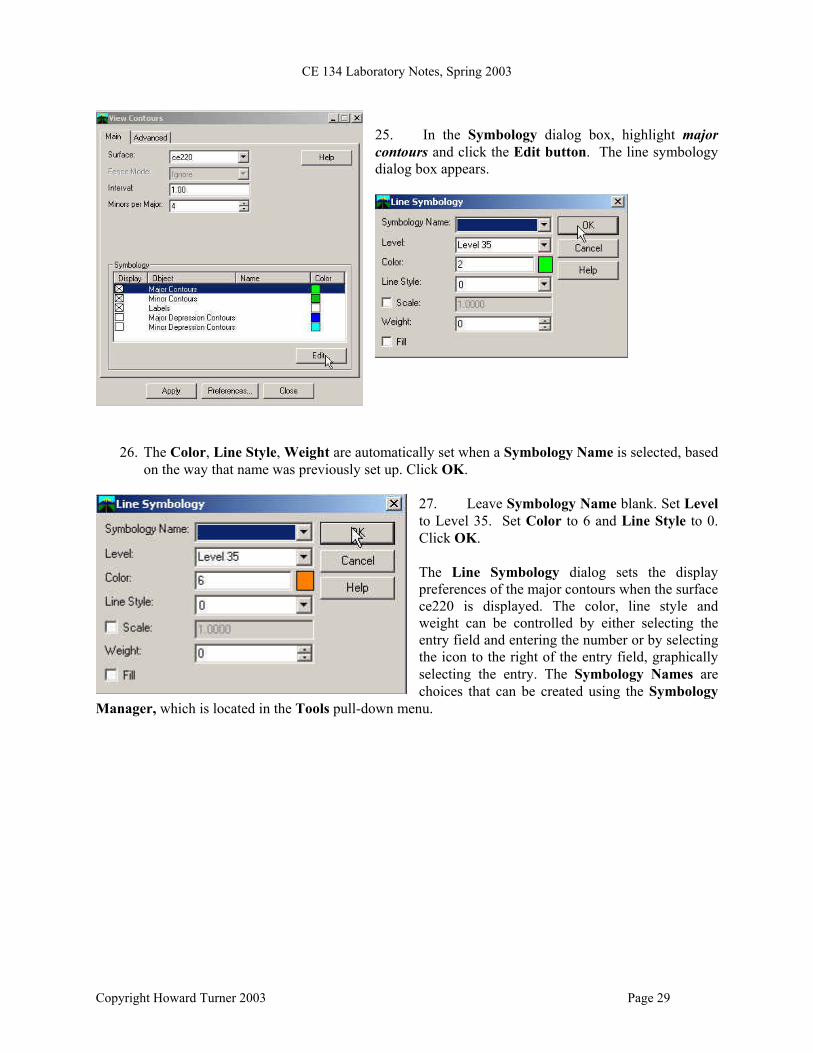
25. In the Symbology dialog box, highlight major contours and click the Edit button. The line symbology dialog box appears.

26. The Color, Line Style, Weight are automatically set when a Symbology Name is selected, based

on the way that name was previously set up. Click OK. 27. Leave Symbology Name blank. Set Level to Level 35. Set Color to 6 and Line Style to 0. Click OK. The Line Symbology dialog sets the display preferences of the major contours when the surface ce220 is displayed. The color, line style and weight can be controlled by either selecting the entry field and entering the number or by selecting the icon to the right of the entry field, graphically selecting the entry. The Symbology Names are choices that can be created using the Symbology

Manager, which is located in the Tools pull-down menu.



Page 30

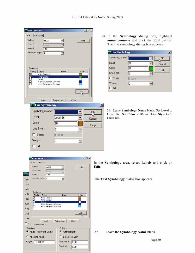
28. In the Symbology dialog box, highlight minor contours and click the Edit button. The line symbology dialog box appears.

Copyright Howard Turner 2003

29. Leave Symbology Name blank. Set Level to Level 36. Set Color to 86 and Line Style to 0. Click OK.

In the Symbology area, select Labels and click on Edit. The Text Symbology dialog box appears. 29. Leave the Symbology Name blank.


Page 31

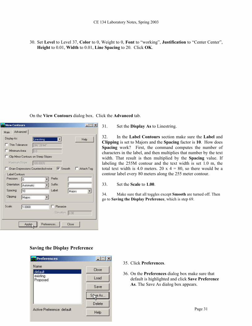
30. Set Level to Level 37, Color to 0, Weight to 0, Font to “working”, Justification to “Center Center”,

Height to 0.01, Width to 0.01, Line Spacing to 20. Click OK. On the View Contours dialog box. Click the Advanced tab.

31. Set the Display As to Linestring. 32. In the Label Contours section make sure the Label and Clipping is set to Majors and the Spacing factor is 10. How does Spacing work? First, the command computes the number of characters in the label, and then multiplies that number by the text width. That result is then multiplied by the Spacing value. If labeling the 255M contour and the text width is set 1.0 m, the total text width is 4.0 meters. 20 x 4 = 80, so there would be a contour label every 80 meters along the 255 meter contour. 33. Set the Scale to 1.00. 34. Make sure that all toggles except Smooth are turned off. Then go to Saving the Display Preference, which is step 69.

Saving the Display Preference

Copyright Howard Turner 2003

35. Click Preferences.

36. On the Preferences dialog box make sure that default is highlighted and click Save Preference As. The Save As dialog box appears.


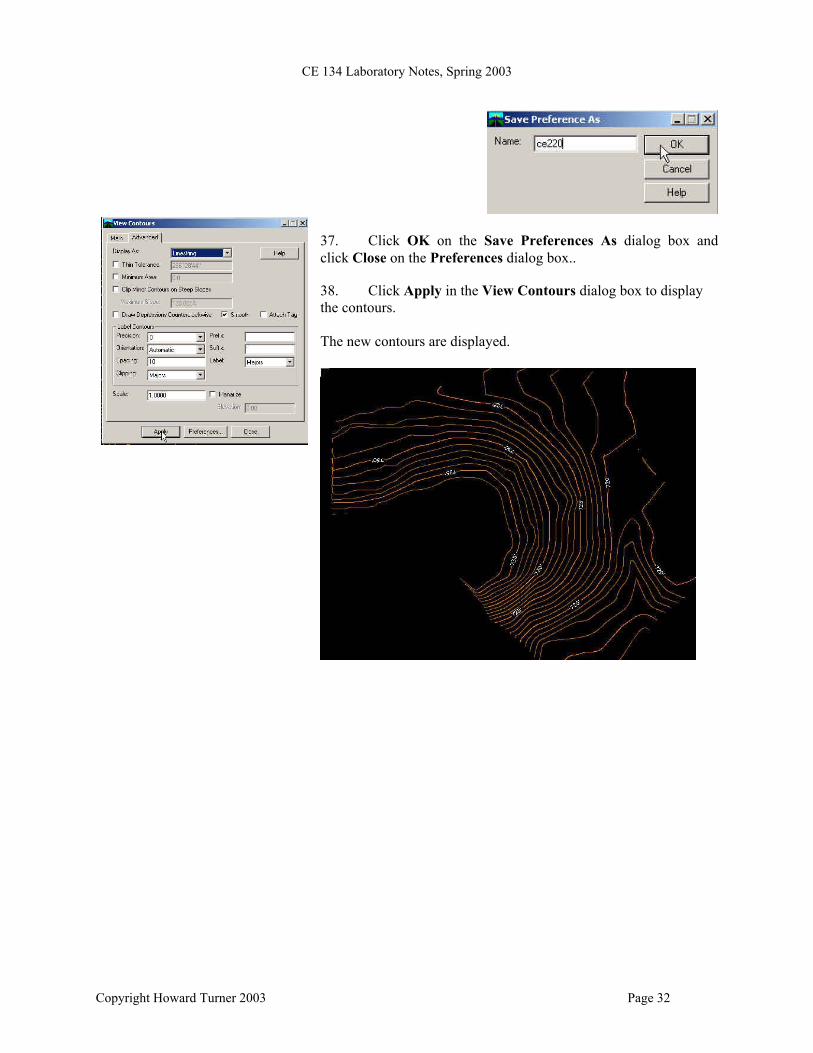
37. Click OK on the Save Preferences As dialog box and click Close on the Preferences dialog box.. 38. Click Apply in the View Contours dialog box to display the contours. The new contours are displayed.



Summary • A DTM can represent any type of spatial data. • Using the File > Import > Surface command is one of the ways to

load data into a surface.

• After the point data is loaded to the surface, the software is used to triangulate the data.

• After the surface is triangulated, save it. Define the location and

name of the surface. • Before displaying the surface terrain contours, it is a good idea to

consider the Write lock and set the Pencil/Pen settings. When the Write lock is turned off, any graphics displayed by InRoads are temporary. However, when the Write lock is on and in Pencil mode, displayed graphics can be zoomed into. If some settings were changed and redisplayed, the old graphics are deleted and replaced by the new graphics.



FINAL MAP SPECIFICATIONS

1. A standard title block shall be used. Examples are available in MicroStation. 2. The map shall be drawn on a "D" size sheet (24"x36") at an appropriate scale ( 1"=20' to 1"=40'). 3. Indicate and describe the corners of the polygon along with the corresponding

elevations. The length and bearing of each side of the polygon shall be shown (bearing over distance or bearing then distance). The basis of bearing for the map shall be shown either in the title block or as a separate note on the map.

4. A rough draft of the topographic map should be reviewed by the instructor during the 9 or 10th week.

5. The final drawing shall be turned in on the last day of lab. The maps will be

graded on accuracy, correctness, neatness, and good general mapping standards.




Documents

CE 134L ELEMENTARY SURVEYING LABORATORY LABORATORY …hturner/ce134/lab2v8.pdf · CE 134 Laboratory Notes, Spring 2003 CE 134L ELEMENTARY SURVEYING LABORATORY LABORATORY # 11 INTRODUCTION