CDF/ANAL/JET/CDFR/3419Version 1.0November 20, 1995Assessing the Signi�cance of a Deviation inthe Tail of a DistributionLuc DemortierThe Rockefeller UniversityAbstractSeveral standard statistical tests can be used to quantify the signi�cance of adeviation in the tail of a measured distribution. We study the bias introduced inthese tests due to binning of the data, variation of the range over which the dataare tested, and systematic uncertainties. Monte Carlo methods to compute correctsigni�cance levels are described. The results are applied to a comparison of the Run1A inclusive jet cross section d�=dET with NLO QCD calculations.1 IntroductionRecently a number of techniques have been proposed to quantify the signi�cance of thediscrepancy at high ET between the measured inclusive jet cross section and the theoreticalprediction [1, 2]. A simple �2-test is not sensitive to the fact that the high-ET bins alldeviate in the same direction from the prediction. On the other hand, there exist empiricaldistribution function tests, such as the Kolmogorov-Smirnov and the Smirnov-Cram�er-von Mises tests, which do have this kind of sensitivity. Like the �2 test, their applicationinvolves the measurement of some deviation statistic S between data and theory, andthe subsequent calculation of a signi�cance level describing the probability to observe adeviation at least as large as S under the hypothesis that data and theory have the sameparent distribution. This calculation can be done with the help of standard subroutinesor tables which were originally derived under several assumptions:1. the tests are performed on unbinned data;2. the range of the tested distribution is not adjusted to optimize the resulting signif-icance level; 1

3. there are no systematic uncertainties;4. the theoretical model does not depend on parameters which are extracted from thedata.The relevance of the �rst three assumptions is to some degree overlooked in reference [2].It is the purpose of this note to study the e�ect of this oversight and to propose a methodto compute correct signi�cance levels. The fourth assumption has already been discussedby Hovhannes Keutelian [3] for the Kolmogorov-Smirnov test, and will not be consideredany further.In section 2 we review the de�nitions of the Kolmogorov-Smirnov and Smirnov-Cram�er-von Mises statistics for both one-sample and two-sample tests. We also describe theAnderson-Darling test [4, 5], which is designed to be more powerful than the �rst twofor detecting deviations in the tail of a distribution. All three of these tests are intendedto be applied to unbinned data. We investigate the e�ect of binning in section 3, anddescribe a method to compute correct signi�cance levels. This method is then applied tothe inclusive jet spectrum in section 4. In section 5, we study what happens to signi�cancelevels when the range of a data distribution is varied until the maximal deviation froma given model is obtained. This technique was actually employed in the inclusive jetanalysis [2], but we show that, when properly applied, it o�ers no additional power overthe standard testing method. A method to incorporate systematic uncertainties in thecomputation of signi�cance levels is described and illustrated in section 6. Our conclusionsare listed in section 7.2 De�nition of some Goodness-of-Fit StatisticsThe goodness-of-�t statistics we are interested in are meant to be applied to the compar-ison of integral distributions, as opposed to the �2 statistic for example, which is appliedto the comparison of distribution densities. Given a set of data points fxi; i = 1; : : : ; Ng,sorted in ascending order, its empirical distribution function is de�ned as follows:SN(x) = 8><>: 0 if x < x1i=N if xi � x < xi+1; i = 1; : : : ; N � 11 if x � xN (1)2.1 One-Sample StatisticsIn order to compare SN (x) to a theoretical distribution F (x), we introduce three statistics:the Kolmogorov-Smirnov statistic Dmax:Dmax def= pN sup�1<x<+1 jSN (x)� F (x)j (2)2

= pN maxi=1;:::;N � yi � i� 1N ; iN � yi � ; (3)where yi def= F (xi), the Smirnov-Cram�er-von Mises statistic W 2:W 2 def= N Z 10 (SN (x)� F (x))2 dF (x) (4)= NXi=1 �yi � 2i� 12N �2 + 112N ; (5)and the Anderson-Darling statistic A2:A2 def= N Z 10 (SN (x)� F (x))2F (x) (1� F (x)) dF (x) (6)= NXi=1 ��2i� 1N � 2� ln(1 � yi) � �2i � 1N � ln(yi)��N : (7)Equalities (5) and (7) were obtained by substituting SN(x) from (1) into (4) and (6)respectively, and integrating separately over each interval over which SN (x) is constant.The statistic A2 is identical toW 2 except for a factor [F (x) (1� F (x))]�1 in the integrand,whose purpose is to give more weight to the tails of the tested distribution. Thus oneexpects the Anderson-Darling statistic to be more powerful at detecting deviations in thetails.2.2 Two-Sample StatisticsIt is sometimes the case that one does not know explicitly the parent distribution functionF (x) of the model with which the data are to be compared. For example, the model couldbe a set of events obtained from a Monte Carlo simulation. One must then compare twoempirical distribution functions, say SN(x) and SM(x). Let us assume that SN (x) isde�ned according to equation (1) from N data events fxi; i = 1; : : : ; Ng, and that SM(x)is similarly de�ned from M Monte Carlo events fyi; i = 1; : : : ;Mg. The two-sampleKolmogorov-Smirnov statistic is:Dmax def= s N MN +M sup�1<x<+1 jSN (x)� SM (x)j (8)The normalization factor in front of the supremum symbol ensures that this Dmax statisticis asymptotically distributed in the same way as the one-sample statistic de�ned by equa-tion (2)1. This way, both statistics should yield asymptotically identical tail probabilities.1The Smirnov theorem guarantees that in the limit M;N !1, with M=N constant, the two-sampleand one-sample Dmax statistics are identically distributed.3

The two-sample W 2 and A2 statistics, to be de�ned below, will be similarly normalized.For this note, we will not attempt to distinguish notationally between one-sample andtwo-sample statistics. What is intended should be clear from the context.In order to �nd the two-sample statistics corresponding to W 2 and A2, we need to �ndsubstitutes for the weight functions dF (x) and dF (x)= [F (x) (1� F (x))] in the integralsof the de�ning equations (4) and (6), since F (x) is not known. The obvious choice isto replace F (x) by S(x), the empirical distribution function formed from both samplescombined. Indeed, under the null-hypothesis that the xi and yi were drawn from the sameparent population, S(x) is our best estimate for F (x). The two-sample Smirnov-Cram�er-von Mises statistic is de�ned by [6]:W 2 def= N MN +M Z 10 (SN (x)� SM (x))2 dS(x) (9)= N M(N +M)2 " NXi=1 (SN (xi)� SM (xi))2 + MXi=1 (SN(yi)� SM(yi))2 # (10)and the two-sample Anderson-Darling statistic by:A2 def= N MN +M Z 10 (SN (x)� SM (x))2S(x) (1 � S(x)) dS(x) (11)= N M(N +M)2 " NXi=1 (SN (xi)� SM (xi))2S(xi) (1 � S(xi)) + MXi=1 (SN(yi)� SM(yi))2S(yi) (1� S(yi)) # (12)In this last expression, one of the sums has a term with a denominator equal to zero,since S(x) = 1 for x = maxfxi; yig. This term has a numerator equal to the square ofzero however, and is therefore left out of the sum.For computational purposes it is convenient to sort the xi and yi in ascending order.Then, if i is the rank of xi in the fxig sample, j the rank of yj in the fyjg sample, andR(z) the rank of z in the combined fxi; yjg sample, we have:SN(xi) = iN SN (yj) = R(yj)� jN (13)SM (xi) = R(xi)� iM SM (yj) = jM (14)S(xi) = R(xi)M +N S(yj) = R(yj)M +N (15)2.3 Tail ProbabilitiesProvided the four conditions listed in the introduction are satis�ed, statistical tests basedon Dmax, W 2 and A2 are distribution-free: under the null-hypothesis, the distributions ofthese statistics do not depend on the form of the tested distribution F (x). This can be4

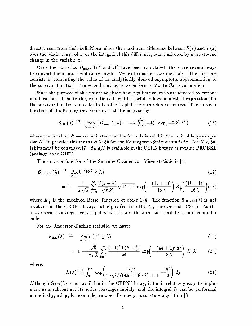
directly seen from their de�nitions, since the maximum di�erence between S(x) and F (x)over the whole range of x, or the integral of this di�erence, is not a�ected by a one-to-onechange in the variable x.Once the statistics Dmax, W 2 and A2 have been calculated, there are several waysto convert them into signi�cance levels. We will consider two methods. The �rst oneconsists in computing the value of an analytically derived asymptotic approximation tothe survivor function. The second method is to perform a Monte Carlo calculation.Since the purpose of this note is to study how signi�cance levels are a�ected by variousmodi�cations of the testing conditions, it will be useful to have analytical expressions forthe survivor functions in order to be able to plot them as reference curves. The survivorfunction of the Kolmogorov-Smirnov statistic is given by:SKS(�) def= ProbN!1 (Dmax � �) = �2 1Xk=1 (�1)k exp(�2 k2 �2 ) (16)where the notation N ! 1 indicates that the formula is valid in the limit of large samplesize N . In practice this means N � 80 for the Kolmogorov-Smirnov statistic. For N < 80,tables must be consulted [7]. SKS(�) is available in the CERN library as routine PROBKL(package code G102).The survivor function of the Smirnov-Cram�er-von Mises statistic is [4]:SSCvM(�) def= ProbN!1 (W 2 � �) (17)= 1� 1�p� 1Xk=0 �(k + 12)p� k! p4k + 1 exp � (4k + 1)216� !K 14 (4k + 1)216� !(18)where K 14 is the modi�ed Bessel function of order 1/4. The function SSCvM(�) is notavailable in the CERN library, but K 14 is (routine BSIR4, package code C327). As theabove series converges very rapidly, it is straightforward to translate it into computercode.For the Anderson-Darling statistic, we have:SAD(�) def= ProbN!1 (A2 � �) (19)= 1 � p8�p� 1Xk=0 (�1)k �(k + 12)k! exp � (4k + 1)2 �28� ! Ik(�) (20)where: Ik(�) def= Z 10 exp �=84� y2= ((4k + 1)2 �2) + 1 � y22 ! dy (21)Although SAD(�) is not available in the CERN library, it too is relatively easy to imple-ment as a subroutine: its series converges rapidly, and the integral Ik can be performednumerically, using, for example, an open Romberg quadrature algorithm [8].5

The advantage of implementing survivor functions in a computer program is that itallows one to calculate tail probabilities outside the range of available tables. However,there are many situations where the asymptotic approximation underlying these formulaeis not valid, for example when the sample size is small, or when the data are binned(see section 3), or when the model depends on parameters which are extracted from thedata. In all these cases, the simplest way to compute tail probabilities is via Monte Carloalgorithms. We illustrate this idea with a procedure to calculate the tail probability of aone-sample statistic:Monte Carlo procedure 1(1) Generate N random numbers xi according to the theoretical distribution F (x), anduse them to form an \empirical" distribution function SN(x).(2) Calculate the one-sample deviation statistic Dmax, W 2 or A2 between F (x) and SN(x).(3) Repeat (1) and (2) a large number of times, and calculate the fraction of times thatthe deviation statistic is larger than the measured one. This is the desired signi�cancelevel of the measurement.Monte Carlo procedures sometimes have a disadvantage, in that large numbers of samplesneed to be generated in order to quantify highly signi�cant deviations. This can becomevery time-consuming. It may be possible to shorten these computations however, usingtechniques such as importance sampling.Figure 1 shows that calculations based on survivor functions or Monte Carlo algorithmsyield identical results in their common domain of applicability. For these plots we ran100,000 Monte Carlo experiments, for each of which we generated 1,000 random data xidistributed according to the density:dFdx = 125x2 ; x 2 [100; 500]: (22)Plots (a), (b) and (c) compare the result of Monte Carlo procedure 1 (data points) with thesurvivor functions (solid lines) for the one-sample Kolmogorov-Smirnov, Smirnov-Cram�er-von Mises, and Anderson-Darling statistics respectively. The agreement is excellent, asexpected.For two-sample tests, the form of the distribution F (x) is not necessarily known, andtherefore step (1) in the above Monte Carlo procedure needs to be modi�ed. As insection 2.2, let us assume that we are to compare a sample of N events with a sampleof M events. The idea is to use the combined sample of N +M events as a \bootstrap"estimator of F (x):Monte Carlo procedure 2(1) Draw N events with replacement from the combined sample of N +M initial events,and form their empirical distribution function SN(x).6

(2) Draw M events with replacement from the combined sample of N +M initial events,and form their empirical distribution function SM(x).(3) Calculate the two-sample deviation statistic Dmax, W 2 or A2 between SN (x) andSM(x).(4) Repeat (1), (2) and (3) a large number of times, and calculate the fraction of timesthat the deviation statistic is larger than the measured one. This is the desired signi�cancelevel of the measurement.Figure 2 checks the equivalence between the above procedure (data points) and the sur-vivor functions (solid lines), for two-sample statistics. The distributions of the two-sampleDmax, W 2 and A2 are plotted for 100,000 trials. For plots (a), (b) and (c), the two initialsamples contained 1,000 events each, drawn according to the density (22). There is goodagreement for the case of W 2 and A2, but a slight shift between the two Dmax distri-butions. As expected (since the advertised equivalence is only asymptotic), this shift isreduced by increasing the size of the initial samples from 1,000 to 4,000 events each (plotd).3 E�ect of Binning the Data SampleIn the case of a complex measurement such as that of the inclusive jet cross sectiond�=dET , one needs to unfold detector e�ects from the measured data, or fold in thosee�ects in the theoretical distribution, before a meaningful comparison between data andtheory can be attempted. The folding or unfolding procedure requires that the data bebinned, and the goodness-of-�t tests described in the previous section must be modi�edin order to be applicable to binned data. Let us assume that the N data points xi arehistogrammed into B bins with contents dj; j = 1; : : : ; B. The empirical distribution isnow given by: Sk = 1N kXj=1 dj ; k = 1; : : : ; B (23)N = BXj=1 dj (24)and is to be compared with:Fk = 1T kXj=1 tj ; k = 1; : : : ; B (25)T = BXj=1 tj (26)tj = F (uj)� F (lj) (27)7

where uk (lk) is the upper (lower) boundary of bin k, and F (x) is the theoretical distri-bution function.3.1 One-Sample Statistics for Binned DataIt is straightforward to translate the de�nitions (2), (4) and (6) in terms of Sk and Fk:Dmax(b) = pN maxk=1;:::;B jSk � Fkj (28)W 2(b) = N B�1Xj=1 (Sj � Fj)2 tjT (29)A2(b) = N B�1Xj=1 (Sj � Fj)2Fj (1 � Fj) tjT (30)where the subscript (b) refers to the fact that we have binned the data before calculatingthese statistics. Note that the sums only need to go up to B � 1 since by de�nitionSB = FB = 1.3.2 Two-Sample Statistics for Binned DataLet fxi; i = 1; : : : ; Ng and fyi; i = 1; : : : ;Mg be two data samples, both histogrammedinto B bins with contents dj and d0j respectively (j = 1; : : : ; B). De�ne the correspondingempirical distribution functions Sk and S 0k according to equation (23). Set d00j = dj + d0j,D00 = PBj=1 d00j , and let S00k be the empirical distribution function for the d00j . The deviationstatistics are then given by:Dmax(b) = s N MN +M maxk=1;:::;B jSk � S0kj (31)W 2(b) = N MN +M B�1Xj=1 �Sj � S0j�2 d00jD00 (32)A2(b) = N MN +M B�1Xj=1 �Sj � S0j�2S 00j (1� S00j ) d00jD00 (33)3.3 Tail Probabilities for Binned DataIn order to be able to convert the statistics Dmax(b), W 2(b) and A2(b) into signi�cance levels,we need to calculate their distributions under the null-hypothesis. It can no longer beassumed that these distributions are given by the survivor functions of section 2.3, exceptin the limit of very �ne binning. The correct distributions are most easily estimated withthe Monte Carlo method, which we illustrate here for the case of one-sample statistics:8

Monte Carlo procedure 3(1) Generate N random numbers xi according to the theoretical distribution F (x) (N isthe number of events in the data sample).(2) Histogram the xi and form the empirical distribution function Sk.(3) Calculate the deviation statistic Dmax(b), W 2(b) or A2(b) between Fk and Sk.(4) Repeat (1) through (3) a large number of times, and calculate the fraction of timesthat the deviation statistic is larger than the measured one. This is the desired signi�cancelevel of the measurement.We have applied this procedure by generating 100,000 Monte Carlo samples of N = 1000events each, distributed according to equation (22). First we histogrammed each MonteCarlo sample in 10 bins from 100 to 500. The resulting distributions of Dmax(b),W 2(b), andA2(b) are plotted as data points in Figure 3. The solid lines in these �gures were calculatedfrom the survivor functions for unbinned statistics. There is a large di�erence betweenthe two calculations. For the case of the Kolmogorov-Smirnov test, binning the testeddistributions tends to reduce the separation between them. Therefore, the signi�canceof a deviation calculated from binned distributions will actually be higher than what thesurvivor functions of section 2.3 predict. The same is true for small deviations in theSmirnov-Cram�er-von Mises and Anderson-Darling tests. For higher values of W 2 and A2however, the data points cross over the solid curves, and deviations become actually lesssigni�cant than what could be expected according to the standard survivor functions.We also tried a �ner binning, 500 bins from 100 to 500, and plotted the result inFigure 4. As expected, the disagreement between binned and unbinned is much less pro-nounced in this case. In conclusion, care is needed when using the standard Kolmogorov-Smirnov, Smirnov-Cram�er-von Mises, or Anderson-Darling distributions to test coarselybinned data. In some sense, this can be contrasted with the �2 test, which requires manyevents per bin in order to be reliable.Monte Carlo procedure 3 is rather impractical in the case of the inclusive jet analysis.The inclusive jet spectrum contains hundreds of thousands of events, and the generationof such a large number of random numbers for each Monte Carlo sample would requirefar too much processing time. In addition, it would be quite di�cult to e�ciently gener-ate random numbers distributed according to the inclusive jet spectrum, because of thecomplexity of the analytical expression which describes this spectrum. Fortunately thereis a trivially simple way to overcome these di�culties:Monte Carlo procedure 4(1) For each bin ti of the theoretical distribution, generate a Poisson uctuation ~ti withmean Nti=T , where N is the number of data events and T =Pi ti. Call Sk the empiricaldistribution formed from the ~ti. 9

(2) Calculate the deviation statistic Dmax(b), W 2(b) or A2(b) between Sk and the theoreticaldistribution Fk.(3) Repeat (1) and (2) a large number of times, and calculate the fraction of times thatthe deviation statistic is larger than the measured one. This is the desired signi�cancelevel of the measurement.This procedure replaces the di�cult generation of N random numbers according to F (x)by the much easier generation of B Poisson random numbers. The equivalence of proce-dures 3 and 4 is illustrated in Figure 5, for the example described above.4 Application to the Inclusive Jet AnalysisWe are now ready to look at the e�ect of binning on the distributions of Dmax(b), W 2(b) andA2(b) for the inclusive jet cross section. The theoretical prediction, smeared for detectore�ects, and the measured data points are listed in table 1 [9]. As the smearing procedureintroduces statistical uncertainties in the theoretical distribution, two-sample statisticsmust be used to test consistency between data and theory.Figure 6 shows the distribution densities of several deviation statistics, as obtained byapplying Monte Carlo procedure 4 (slightly modi�ed to handle two-sample statistics) tothe theoretical prediction for the inclusive jet cross section. The densities obtained bydi�erentiating the standard survivor functions are also shown for comparison. As morebins are included in the calculation of a statistic, the distribution of that statistic becomesmore like that of the corresponding asymptotic survivor function.A quantitative comparison between data and theory is provided in table 2. The signif-icance levels are expressed as numbers of standard deviations for a Gaussian distribution,which are somewhat easier to comprehend than probabilities, especially when the latterare very small. The correspondence between probabilities P and numbers of standarddeviations r is given by:P def= Prob(jXj � r) = 2p2� Z r�1 e� t22 dt (34)where X is a normal variate. The table also provides the results of a standard �2 testof goodness of �t. For two histograms with bin contents fdi; i = 1; : : : ; Bg and fd0i; i =1; : : : ; Bg, summing up to D and D0 respectively, the variable:X2 def= BXi=1 �diqD0=D � d0iqD=D0�2di + d0i (35)is approximately distributed as a �2 variable with B � 1 degrees of freedom.10

Bin Jet ET Number of events Bin Jet ET Number of events(GeV) Theory Data (GeV) Theory Data1 14.6 1841 1691 22 133.8 8738 87092 20.4 423 367 23 139.2 6759 67823 26.9 110969 99263 24 144.5 5227 51274 33.3 43435 41677 25 149.9 4071 40185 39.5 19176 19139 26 155.3 3156 32126 45.5 9677 9505 27 160.6 2472 25207 51.3 5165 5182 28 168.4 3534 35758 57.0 2933 2844 29 179.2 2245 22429 62.7 1757 1746 30 189.9 1457 149810 68.3 1088 1105 31 200.7 972 104411 73.9 689 662 32 211.5 638 69512 79.5 456 420 33 224.7 586 68313 85.0 6350 6165 34 241.0 327 34414 90.5 4405 4362 35 257.4 186 20115 95.9 3076 2979 36 273.8 107 12916 101.4 2216 2224 37 292.5 77 9817 106.8 6276 6203 38 314.4 38 5218 112.2 4584 4499 39 336.2 19 2419 117.6 3379 3409 40 365.5 14 2120 123.0 2525 2522 41 418.5 4 1021 128.4 1899 1876Table 1: Inclusive jet event rate, smeared NLO QCD theory and raw data, as a functionof jet ET .11

Deviation Bin Value of Standard Corrected Smeared S.L.Statistic Range Statistic S.L. S.L. �stab = 1% �stab = 2:5%5{41 38.2/36 0.90 0.90 0.65 0.5310{41 35.9/31 1.15 1.15 0.95 0.7915{41 30.9/26 1.19 1.19 1.00 0.87�2=Ndof 20{41 26.8/21 1.35 1.36 1.18 1.0625{41 21.5/16 1.41 1.41 1.27 1.1730{41 10.2/11 0.65 0.64 0.60 0.5835{41 3.65/6 0.35 0.34 0.34 0.335{41 1.201 1.59 1.86 1.32 0.9010{41 1.395 2.05 2.38 1.67 1.2715{41 1.356 1.96 2.34 1.74 1.40Dmax(b) 20{41 1.324 1.88 2.32 1.88 1.6025{41 1.335 1.91 2.41 2.02 1.8230{41 0.923 0.91 1.52 1.39 1.3135{41 0.659 0.28 0.99 0.97 0.965{41 0.616 2.32 2.25 1.59 1.0810{41 1.025 3.07 3.06 1.99 1.4815{41 0.802 2.69 2.65 1.86 1.48W 2(b) 20{41 0.770 2.63 2.50 1.96 1.6625{41 0.915 2.89 2.77 2.24 1.9930{41 0.579 2.24 2.01 1.82 1.7135{41 0.328 1.59 1.39 1.36 1.345{41 4.540 2.82 2.75 1.81 1.2510{41 6.808 3.54 3.52 2.18 1.6115{41 5.633 3.19 3.15 2.10 1.65A2(b) 20{41 5.239 3.06 2.97 2.20 1.8525{41 5.802 3.24 3.12 2.43 2.1330{41 3.060 2.23 2.09 1.86 1.7335{41 1.667 1.47 1.39 1.36 1.33Table 2: Signi�cance levels obtained from a comparison between inclusive jet data andtheory. Values and signi�cance levels are given for each of four di�erent deviation statisticsand for several ET bin ranges. The bin numbers refer to table 1. Signi�cance levelsare expressed in equivalent numbers of standard deviations for a Gaussian distribution.Standard signi�cance levels (column 4) were obtained from asymptotic survivor functions,whereas the corrected signi�cance levels (column 5) were computed according to MonteCarlo procedure 4 (one million trials). The last two columns incorporate the e�ect of allthe systematic uncertainties (cfr. section 6). The uncertainty on the ET scale stabilitywas taken to be 1% for column 6, and 2.5% for column 7 (see [2]).12

Several points can be made about the results shown in the table. Except for the �2statistic, there is a clear di�erence between the signi�cance levels computed from thestandard survivor functions, and those obtained from the correct Monte Carlo procedurefor binned data. The di�erence is most pronounced in the case of Dmax(b). It is alsoevident that A2(b) is more powerful at detecting deviations than W 2(b), which is itself morepowerful than Dmax(b). The �2 statistic is the weakest of all four. Finally, the deviationdetected by these statistics is indeed in the tail of the jet ET distribution, since thesigni�cance levels do not change much as the �rst bin in the tested bin range moves frombin 5 to bin 25. Beyond bin 30, the signi�cances start to decrease because by then thehigh-statistics central region of the jet ET distribution is no longer available to \calibrate"the comparison of data with theory.Another way to demonstrate that the observed deviation comes from high-ET jets isto compare theory and data in the central region of the spectrum, leaving out the tail.This is done in table 3, where each of the four deviation tests is applied to the ET regionbetween bins 5 and 25. In all cases, data and theory are within 0.2 standard deviationsof each other.Deviation Bin Value of Standard Corrected Smeared S.L.Statistic Range Statistic S.L. S.L. �stab = 1% �stab = 2:5%�2=Ndof 5{25 7.9/20 0.0093 0.0092 0.0058 0.0050Dmax(b) 5{25 0.358 0.00058 0.047 0.027 0.024W 2(b) 5{25 0.052 0.171 0.18 0.11 0.09A2(b) 5{25 0.285 0.064 0.15 0.087 0.076Table 3: Signi�cance levels obtained from a comparison between data and theory of thecentral region (bins 5 through 25) of the inclusive jet ET spectrum. These signi�cancelevels are expressed in numbers of standard deviations for a Gaussian distribution. Thecolumns in this table have the same meaning as in table 2.5 E�ect of Varying the Range of the Tested Distri-butionSince our goal is to quantify a deviation between data and theory in the tail of the jet ETspectrum, it may be tempting to try the following procedure [2]:1. Test all bin ranges of the form i{41, where i is a bin number between 1 and 40;2. Select the range which gives the largest deviation statistic (Dmax(b), W 2(b) or A2(b));13

3. Convert the value of the deviation statistic into a signi�cance level.The third step requires some care. We are no longer doing standard Kolmogorov-Smirnov,Smirnov-Cram�er-von Mises or Anderson-Darling tests as described in section 2, since weare optimizing the bin range, thereby introducing another random variable in addition tothe deviation statistic itself. Let us therefore rename the deviation statistics obtained bythe above procedure Dmaxmax(b), W 2(b)max and A2(b)max. Using a simple and obvious modi�ca-tion of Monte Carlo procedure 4, we can plot distributions of the new statistics. This isshown in Figure 7, for the case of the inclusive jet analysis. There is a large di�erencebetween these distributions and the distributions of the standard statistics. The resultsof testing the deviation between data and theory are listed in table 4. They indicate thatthis method is actually less powerful than the simpler tests investigated in the previoussection.Deviation Statistic Value Bin range for which Standard S.L. Corrected S.L.value is reachedDmaxmax(b) 1.448 28{41 2.17 1.54W 2(b)max 1.236 24{41 3.39 1.99A2(b)max 7.438 24{41 3.71 2.47Table 4: Signi�cance levels obtained from a comparison between inclusive jet data and the-ory. The deviation statistics are de�ned in the text. The signi�cance levels are expressedin numbers of standard deviations for a Gaussian distribution. Standard signi�cance levelswere computed from the survivor functions for Dmax, W 2 and A2, whereas the correctedsigni�cance levels were obtained from a Monte Carlo procedure.6 E�ect of Systematic UncertaintiesSo far we have not incorporated the e�ect of systematic uncertainties in the evaluation ofsigni�cance levels. This is fairly straightforward to do when the �2 statistic is used; seefor example [10]. For the case of the Dmax, W 2 and A2 statistics, binned or unbinned, adi�erent procedure must be adopted.For binned data, the following method has been suggested in [2]. First, one adjusts thesystematics to obtain the best possible agreement between data and theoretical model.This adjustment is driven by a least-squares algorithm which incorporates the e�ect ofsystematic uncertainties. It allows for some limited variation in shape of the �tted dis-tribution. Any remaining shape di�erence between data and theory is then subsequentlypicked up by a shape-sensitive test based on Dmax, W 2 or A2.14

While this method will certainly yield a signi�cance which is diluted by systematice�ects, it is not at all clear that the least-squares algorithm will converge to the sameminimum as an algorithm whose goodness-of-�t criterion is Dmax, W 2 or A2. Therefore,it is also not clear whether the �nal signi�cance properly takes into account the full rangeof systematic e�ects.We propose here a method which avoids the above di�culty by calculating signi�cancelevels from smeared distributions of the deviation statistics. The smearing proceduresamples the whole range of systematics with the appropriate weighting function. Let usassume we are to compare a data histogram fdig with a model histogram fmig, and thatboth model and data are subject to statistical uctuations:Monte Carlo procedure 5(1) For each bin of the model distribution, generate a Poisson uctuation ~mi with meanmi. Call Sk the empirical distribution formed from the ~mi.(2) Create a \systematic" uctuation fm0ig of the model histogram. For example, if thereis only one systematic uncertainty, which is Gaussian and fully correlated across bins, onewould generate a single normal random number X, and shift each bin mi by the amountX � �i, where �i is the absolute systematic uncertainty on the contents mi. If there areseveral systematic uncertainties, several such shifts will have to be done.(3) For each bin of the histogram obtained from step (2), generate a Poisson uctuation~m0i with mean m0i. Let S0k be the empirical distribution function associated with the ~m0i.(4) Calculate the deviation statistic Dmax(b), W 2(b) or A2(b) between Sk and S0k.(5) Repeat steps (1), (2), (3) and (4) a large number of times, and calculate the fractionof times that the deviation statistic is larger than the measured one. This is the desiredsigni�cance level of the measurement, smeared with systematic e�ects.We have applied this procedure to the inclusive jet data of section 4. The inclusive jetanalysis considers a total of eight systematic uncertainties. Since these uncertainties areindependent and act in the same way on the jet ET spectrum, it is su�cient to considera single systematic uncertainty, equal to the bin-by-bin sum in quadrature of the originaleight [1]. We will consider two cases. For the �rst case, the uncertainty on the stability ofthe absolute calibration of the calorimeter, �stab, is assumed to be 1%. This is consideredto be a correct assumption [2], and leads to a combined systematic uncertainty varyingfrom about 13% at low ET to about 28% at high ET . For the second case, the uncertaintyon the stability of the calibration is set to its upper limit of 2.5%. Here, the combinedsystematic uncertainty varies from about 17% to 39%. The results of our calculations aregiven in the last two columns of tables 2 and 3.Table 2 shows that the statistic A2(b), calculated from bins 10 through 41, gives thehighest signi�cance: 3.52 standard deviations. When using Monte Carlo procedure 515

with the combined systematic uncertainty, we �nd smeared signi�cances of 2.18 and 1.61standard deviations, depending on the assumption about the stability of the calibrationof the calorimeter. Although this result may seem disappointing, it should not come asa surprise. Figure 8 shows how the value of A2(b), calculated from bins 10 through 41,varies as a function of the amount of systematic uncertainty added to the theoreticaldistribution. This amount is measured in numbers of standard deviations of systematicuncertainty. Horizontal lines in the plot indicate the signi�cance levels corresponding tovarious values of A2(b). For �stab = 1% or 2:5%, shifting the theoretical distribution byabout 2.6, respectively 1.1 standard deviations of systematic uncertainty brings it withinless than one standard deviation of the data. This plot illustrates that, with the givensystematic uncertainty, data and theory are not very far from each other, and that theshape of the systematic uncertainty can easily accomodate the high-ET excess observedin the data.7 ConclusionsWe have reviewed the formalism of one-sample and two-sample tests with the Kolmogorov-Smirnov, Smirnov-Cram�er-von Mises, and Anderson-Darling statistics. When the testeddistribution is coarsely binned, as is the case for the inclusive jet ET spectrum, we haveshown that correct signi�cance levels can not be obtained from standard published tablesor subroutines, but can be calculated with Monte Carlo algorithms, of which we gaveseveral examples. Applying this technique to the inclusive jet ET spectrum, we found thatthe Anderson-Darling test is more powerful than the other two at detecting deviationsin the tail of the spectrum. We then studied the e�ect of choosing the range of binsto include in a given test. When the criterion guiding this choice is the maximizationof the discrepancy between two distributions, the corresponding signi�cance levels arestrongly biased, as one should expect. Finally, we proposed a Monte Carlo procedureto incorporate the e�ect of systematic uncertainties into the tests, and applied it to theinclusive jet ET spectrum.16

References[1] Anwar Ahmad Bhatti, \A Few Minor Points in Inclusive Jet Cross Section", QCDGroup Meeting of September 14, 1995;Tom Devlin, \Jet Inclusive Cross Sections: Statistical Issues", QCD Group Meetingof September 14, 1995.[2] Tom Devlin, \Jet Inclusive Cross Sections: A Statistical Study of the `Excess' ", CDFnote 3301, Version 3.0 (October 1, 1995).[3] Hovhannes Keutelian, \The Kolmogorov-Smirnov Test when Parameters are Esti-mated from Data", CDF note 1285, Version 1.0 (April 30, 1991).[4] T.W. Anderson and D.A. Darling, \Asymptotic Theory of Certain `Goodness of Fit'Criteria Based on Stochastic Processes", Ann. Math. Stat. 23, 193-212 (1952).[5] T.W. Anderson and D.A. Darling, \A Test of Goodness of Fit", J. Amer. Stat. Assoc.49, 765-769 (1954).[6] Integration with respect to a discrete distribution function is discussed in many stan-dard texts on probability; see for example section 4.2.2 in: A.F. Karr, \Probability",Springer-Verlag, 1993, 282pp.[7] Byron P. Roe, \Probability and Statistics in Experimental Physics", Springer-Verlag,1992, 208pp.[8] W.H. Press, S.A. Teukolsky, W.T. Vetterling, B.P. Flannery, \Numerical Recipes inFORTRAN, The Art of Scienti�c Computing", Second Edition, Cambridge Univer-sity Press, 1992, 963 pp.[9] Anwar Ahmad Bhatti, private communication. In all our calculations, we have leftout the four bins at lowest ET . These make a large contribution to a �2 goodness-of-�ttest, and don't a�ect the study of the high-ET excess (see [2]).[10] T. Devlin, \Correlations from Systematic Corrections to Poisson-Distributed Datain Log-Likelihood Functions", CDF note 3126, Version 3.0 (August 19, 1995).17

Figure 1: Distributions of (a) the Kolmogorov-Smirnov statistic, (b) the Smirnov-Cram�er-von Mises statistic, and (c) the Anderson-Darling statistic for one-sample tests on un-binned data. The data points are histograms obtained by generating 100,000 trials ac-cording to Monte Carlo procedure 1. The solid lines are the result of numerically di�er-entiating the survivor functions SKS, SSCvM and SAD respectively, and are normalizedto the same areas as the corresponding histograms.18

Figure 2: Distributions of the two-sample Kolmogorov-Smirnov statistic (plots a and d),Smirnov-Cram�er-von Mises statistic (b), and Anderson-Darling statistic (c) for unbinneddata. The data points are histograms obtained by generating 100,000 trials according toMonte Carlo procedure 2. For plots (a), (b) and (c), the initial samples contained 1,000events each, whereas for plot (d) they contained 4,000 events each. The solid lines arethe result of numerically di�erentiating the survivor functions SKS, SSCvM, SAD and SKSrespectively, and are normalized to the same areas as the corresponding histograms.19

Figure 3: Distributions of (a) the Kolmogorov-Smirnov statistic, (b) the Smirnov-Cram�er-von Mises statistic, and (c) the Anderson-Darling statistic for one-sample tests on coarselybinned data (see text). The data points are histograms obtained by generating 100,000trials according to Monte Carlo procedure 3. The solid lines are the result of numer-ically di�erentiating the survivor functions SKS, SSCvM and SAD respectively, and arenormalized to the same areas as the corresponding histograms.20

Figure 4: Distributions of (a) the Kolmogorov-Smirnov statistic, (b) the Smirnov-Cram�er-von Mises statistic, and (c) the Anderson-Darling statistic for one-sample tests on �nelybinned data (see text). The data points are histograms obtained by generating 100,000trials according to Monte Carlo procedure 3. The solid lines are the result of numer-ically di�erentiating the survivor functions SKS, SSCvM and SAD respectively, and arenormalized to the same areas as the corresponding histograms.21

Figure 5: Distributions of the one-sample Kolmogorov-Smirnov statistic (a), Smirnov-Cram�er-von Mises statistic (b), and Anderson-Darling statistic (c) for the density repre-sented by equation (22), histogrammed in 10 bins from 100 to 500. The histograms wereobtained with Monte Carlo procedure 3, the data points with procedure 4.22

Figure 6: Distributions of the two-sample Kolmogorov-Smirnov statistic (a), Smirnov-Cram�er-von Mises statistic (b), and Anderson-Darling statistic (c) for the ET -binned run1A inclusive jet sample (cfr. table 1). The dashed and dotted histograms were obtained byusing bins 5 through 41, respectively 30 through 41, to calculate the statistics. The solidlines are the result of numerically di�erentiating the survivor functions SKS, SSCvM andSAD respectively, and are normalized to the same areas as the corresponding histograms.23

Figure 7: The dashed histograms are distributions of the two-sample deviation statisticsDmaxmax(b) (plot a), W 2(b)max (plot b), and A2(b)max (plot c) for the ET -binned run 1A inclu-sive jet sample. The solid lines are the result of numerically di�erentiating the survivorfunctions SKS, SSCvM and SAD respectively, and are normalized to the same areas as thecorresponding histograms. 24

Figure 8: Comparison of inclusive jet data and theory: the two curves show the variationof the statistic A2(b) as a function of the number of standard deviations of systematicuncertainty added to the theoretical distribution. The uncertainty on the stability ofthe absolute calibration of the calorimeter was set to 1% (dashed curve) and 2.5% (solidcurve). The dotted horizontal lines show various signi�cance levels associated with givenvalues of A2(b). 25