CDA6530: Performance Models of Computers and Networks

Chapter 2: Review of Practical Random Variables

2

Two Classes of R.V.

Discrete R.V. Bernoulli Binomial Geometric Poisson

Continuous R.V. Uniform Exponential, Erlang Normal

Closely related Exponential Geometric Normal Binomial, Poisson

3

Definition

Random variable (R.V.) X: A function on sample space X: S ! R

Cumulative distribution function (CDF): Probability distribution function (PDF) Distribution function FX(x) = P(X ≤ x) Can be used for both continuous and discrete

random variables

Probability density function (pdf): Used for continuous R.V.

Probability mass function (pmf): Used for discrete R.V. Probability of the variable exactly equals to a

value

4

FX (x) =Rx¡ 1 f X (t)dt f X (x) = dFX (x)

dx

5

Bernoulli

A trial/experiment, outcome is either “success” or “failure”. X=1 if success, X=0 if failure P(X=1)=p, P(X=0)=1-p

Bernoulli Trials A series of independent repetition of Bernoulli

trial.

6

Binomial

A Bernoulli trials with n repetitions Binomial: X = No. of successes in n trails

X» B(n, p)P (X = k) ´ f (k; n;p) =

Ãnk

!

pk(1 ¡ p)n¡ k

where Ã

nk

!

= n!(n¡ k)!k!

7

Binomial Example (1)

A communication channel with (1-p) being the probability of successful transmission of a bit. Assume we design a code that can tolerate up to e bit errors with n bit word code.

Q: Probability of successful word transmission? Model: sequence of bits trans. follows a Bernoulli Trails

Assumption: each bit error or not is independent P(Q) = P(e or fewer errors in n trails) =

P ei=0 f (i; n;p)

=P e

i=0

Ãni

!

pi(1 ¡ p)n¡ i

Introduction 1-8

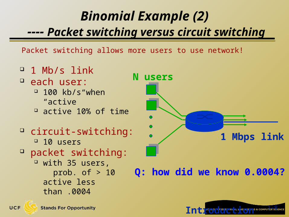
Binomial Example (2) ---- Packet switching versus circuit switching

1 Mb/s link each user:

100 kb/s when “active” active 10% of time

circuit-switching: 10 users

packet switching: with 35 users, prob. of > 10 active less

than .0004

Packet switching allows more users to use network!

N users

1 Mbps link

Q: how did we know 0.0004?

9

Geometric

Still about Bernoulli Trails, but from a different angle.

X: No. of trials until the first success Y: No. of failures until the first success P(X=k) = (1-p)k-1p P(Y=k)=(1-p)kp

X Y

10

Poisson

Limiting case for Binomial when: n is large and p is small

n>20 and p<0.05 would be good approximation Reference: wiki

¸=np is fixed, success rate X: No. of successes in a time interval (n time

units)

Many natural systems have this distribution The number of phone calls at a call center per minute. The number of times a web server is accessed per minute. The number of mutations in a given stretch of DNA after a

certain amount of radiation.

P (X = k) = e¡ ¸ ¸k

k!

11

Continous R.V - Uniform

X: is a uniform r.v. on (®, ¯) if

Uniform r.v. is the basis for simulation other distributions Introduce later

f (x) =

8<

:

1¯ ¡ ®; if®< x < ¯

0 otherwise

12

Exponential

r.v. X:

FX(x)= 1-e-¸ x

Very important distribution Memoryless property Corresponding to geometric

distr.

f (x) =

8<

:¸e¡ ¸x; if x ¸ 00 if x < 0

13

Erlang

r.v. X (k-th Erlang):

K-th Erlang is the sum of k Exponential distr.

14

Normal

r.v. X:

Corresponding to Binomial and Poisson distributions

15

Normal

If X~N(¹, ¾2), then r.v. Z=(X-¹)/¾ follows standard normal N(0,1) P(Z<x) is denoted as ©(x)

©(x) value can be obtained from standard normal distribution table (next slide)

Used to calculate the distribution value of a normal random variable X~N(¹, ¾2)

P(X<®) = P(Z < (®-¹)/¾) = ©( (®-¹)/¾ )

16

Standard Normal Distr. Table

P(X<x) = ©(x) ©(-x) = 1- ©(x) why? About 68% of the area under the curve falls within 1

standard deviation of the mean. About 95% of the area under the curve falls within 2

standard deviations of the mean. About 99.7% of the area under the curve falls within 3

standard deviations of the mean.

17

Normal Distr. Example

An average light bulb manufactured by Acme Corporation lasts 300 days, 68% of light bulbs lasts within 300+/- 50 days. Assuming that bulb life is normally distributed.

Q1: What is the probability that an Acme light bulb will last at most 365 days?

Q2: If we installed 100 new bulbs on a street exactly one year ago, how many bulbs still work now on average? What is the distribution of the number of remaining bulbs?

Step 1: Modeling X~N(300, 502) ¹=300, ¾=50. Q1 is P(X· 365) define Z = (X-300)/50, then Z is standard normal For Q2, # of remaining bulbs, Y, is a Bernoulli trial with 100

repetitions with small prob. p = [1- P(X · 365)] Y follows Poisson distribution (approximated from Binomial distr.) E[Y] = λ= np = 100 * [1- P(X · 365)]

18

Memoryless Property

Memoryless for Geometric and Exponential Easy to understand for Geometric

Each trial is independent how many trials before hit does not depend on how many times I have missed before.

X: Geometric r.v., PX(k)=(1-p)k-1p; Y: Y=X-n No. of trials given we failed first n times PY(k) = P(Y=k|X>n)=P(X=k+n|X>n)

= P (X =k+n;X >n)P (X >n) = P (X =k+n)

P (X >n)

= (1¡ p)k+n¡ 1p(1¡ p)n = p(1 ¡ p)k¡ 1 = PX (k)

19

pdf: probability density function Continuous r.v. fX(x)

pmf: probability mass function Discrete r.v. X: PX(x)=P(X=x) Also denoted as PX(x) or simply P(x)

20

Mean (Expectation)

Discrete r.v. X E[X] = kPX(k)

Continous r.v. X E[X] =

Bernoulli: E[X] = 0(1-p) + 1¢ p = p Binomial: E[X]=np (intuitive meaning?) Geometric: E[X]=1/p (intuitive meaning?) Poisson: E[X]=¸ (remember ¸=np)

Z 1

¡ 1kf (k)dk

21

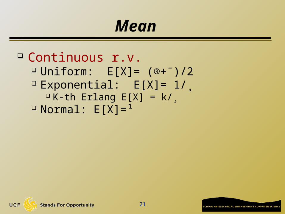
Mean

Continuous r.v. Uniform: E[X]= (®+¯)/2 Exponential: E[X]= 1/¸

K-th Erlang E[X] = k/¸ Normal: E[X]=¹

22

Function of Random Variables

R.V. X, R.V. Y=g(X) Discrete r.v. X:

E[g(X)] = g(x)p(x) Continuous r.v. X:

E[g(X)] =

Variance: Var(X) = E[ (X-E[X])2 ] = E[X2] – (E[X])2

Z 1

¡ 1g(x)f (x)dx

23

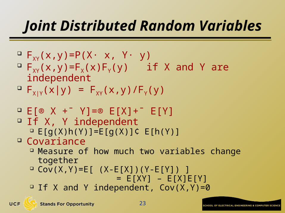
Joint Distributed Random Variables

FXY(x,y)=P(X· x, Y· y) FXY(x,y)=FX(x)FY(y) if X and Y are independent FX|Y(x|y) = FXY(x,y)/FY(y)

E[® X +¯ Y]=® E[X]+¯ E[Y] If X, Y independent

E[g(X)h(Y)]=E[g(X)]¢ E[h(Y)] Covariance

Measure of how much two variables change together Cov(X,Y)=E[ (X-E[X])(Y-E[Y]) ] = E[XY] – E[X]E[Y] If X and Y independent, Cov(X,Y)=0

24

Limit Theorems - Inequality

Markov’s Inequality r.v. X¸ 0: 8 ®>0, P(X¸ ®) · E[X]/®

Chebyshev’s Inequality r.v. X, E[X]=¹, Var(X)=¾2

8 k>0, P(|X-¹|¸ k)· ¾2/k2

Provide bounds when only mean and variance known The bounds may be more conservative than

derived bounds if we know the distribution

25

Inequality Examples

If ®=2E[X], then P(X¸®)· 0.5 A pool of articles from a publisher. Assume we know

that the articles are on average 1000 characters long with a standard deviation of 200 characters.

Q: what is the prob. a given article is between 600 and 1400 characters?

Model: r.v. X: ¹=1000, ¾=200, k=400 in Chebyshev’s P(Q) = 1- P(|X-¹|¸ k) ¸ 1- (¾/k)2 =0.75

If we know X follows normal distr.: The bound will be tigher 75% chance of an article being between 760 and

1240 characters long

26

Strong Law of Large Number

i.i.d. (independent and identically-distributed) Xi: i.i.d. random variables, E[Xi]=¹

With probability 1, (X1+X2+ +Xn)/n ¹, as n1

Foundation for using large number of simulations to obtain average results

27

Central Limit Theorem

Xi: i.i.d. random variables, E[Xi]=¹ Var(Xi)=¾2

Y=

Then, Y » N(0,1) as n1 The reason for why normal distribution is everywhere Sample mean is also normal distributed

Sample mean

X 1 + X 2 + ¢¢¢+ X n ¡ n¹¾

pn

¹X =nX

i=1X i=n

E [ ¹X ] = ¹V ar( ¹X ) = ¾2=n

What does this mean?

¹X

28

Example

Let Xi, i=1,2,, 10 be i.i.d., Xi is uniform distr. (0,1). Calculate

E[Xi]=0.5, Var(Xi)=1/12

P (10X

i=1X i > 7)

P (10X

i=1X i > 7) = P (

P 10i=1 X i ¡ 5

q10(1=12)

>7 ¡ 5

q10(1=12)

)

¼1 ¡ ©(2:2) = 0:0139

©(x): prob. standard normal distr. P(X< x)

29

Conditional Probability

Suppose r.v. X and Y have joint pmf p(x,y) p(1,1)=0.5, p(1,2)=0.1, p(2,1)=0.1, p(2,2)=0.3 Q: Calculate the pmf of X given that Y=1

pY(1)=p(1,1)+p(2,1)=0.6 X sample space {1,2} pX|Y (1|1) =P(X=1|Y=1) = P(X=1, Y=1)/P(Y=1)

= p(1,1)/pY(1) = 5/6

Similarly, pX|Y(2,1) = 1/6

30

Expectation by Conditioning

r.v. X and Y. then E[X|Y] is also a r.v. Formula: E[X]=E[E[X|Y]]

Make it clearer, EX[X]= EY[ EX[X|Y] ] It corresponds to the “law of total probability”

EX[X]= EX[X|Y=y] ¢ P(Y=y) Used in the same situation where you use the law

of total probability

31

Example

r.v. X and N, independent Y=X1+X2+ +XN

Q: compute E[Y]?

32

Example 1

A company’s network has a design problem on its routing algorithm for its core router. For a given packet, it forwards correctly with prob. 1/3 where the packet takes 2 seconds to reach the target; forwards it to a wrong path with prob. 1/3, where the packet comes back after 3 seconds; forwards it to another wrong with prob. 1/3, where the packet comes back after 5 seconds.

Q: What is the expected time delay for the packet reach the target?

Memoryless Expectation by condition

33

Example 2

Suppose a spam filter gives each incoming email an overall score. A higher score means the email is more likely to be spam. By running the filter on training set of email (known normal + known spam), we know that 80% of normal emails have scores of 1.5 0.4; 68% of spam emails have scores of 4 1. Assume the score of normal or spam email follows normal distr.

Q1: If we want spam detection rate of 95%, what threshold should we configure the filter?

Q2: What is the false positive rate under this configuration?

34

Example 3

A ball is drawn from an bottle containing three white and two black balls. After each ball is drawn, it is then placed back. This goes on indefinitely. Q: What is the probability that among the first

four drawn balls, exactly two are white?

P (X = k) ´ f (k; n;p) =

Ãnk

!

pk(1 ¡ p)n¡ k

35

Example 4

A type of battery has a lifetime with ¹=40 hours and ¾=20 hours. A battery is used until it fails, at which point it is replaced by a new one.

Q: If we have 25 batteries, what’s the probability that over 1100 hours of use can be achieved?

Approximate by central limit theorem

36

Example 5

If the prob. of a person suffer bad reaction from the injection of a given serum is 0.1%, determine the probability that out of 2000 individuals (a). exactly 3 (b). More than 2 individuals suffer a bad reaction? (c). If we inject one person per minute, what is the average time between two bad reaction injections?

Poisson distribution (for rare event in a large number of independent event series)

Can use Binomial, but too much computation Geometric

37

Example 6

A group of n camping people work on assembling their individual tent individually. The time for a person finishes is modeled by r.v. X. Q1: what is the PDF for the time when the first tent is

ready? Q2: what is the PDF for the time when all tents are

ready?

Suppose Xi are i.i.d., i=1, 2, , n Q: compute PDF of r.v. Y and Z where

Y= max(X1, X2, , Xn) Z= min(X1, X2, , Xn) Y, Z can be used for modeling many phenomenon

38

Example 7

A coin having probability p of coming up heads is flipped until two of the most recent three flips are heads. Let N denote the number of heads. Find E[N].

P(N=n) = P(Y2¸ 3, , Yn-1¸ 3, Yn· 2)

0 0 0 1 0 0 0 0 1 0 0 1 0 1