Embed Size (px)
Citation preview

CCSP SAP 3.4 – Chapter 4 October 24, 2007
Chapter 4 1 2 3 4 5 6 7 8 9
10 11 12 13 14 15 16 17 18 19 20 21 22 23 24 25 26 27 28 29 30 31 32 33 34 35 36 37 38 39 40 41 42 43 44
The Potential for Abrupt Change in the Atlantic Meridional
Overturning Circulation Chapter Lead Author: Thomas L. Delworth* Contributing Authors: Peter Clark,* Marika Holland, Bill Johns, Till Kuhlbrodt, Jean Lynch-Stieglitz, Carrie Morrill,* Richard Seager,* Andrew Weaver,* and Rong Zhang *SAP 3.4 FACA Committee Member
KEY FINDINGS The Atlantic Meridional Overturning Circulation (AMOC) is an important component of the Earth’s climate system, characterized by a northward flow of warm, salty water in the upper layers of the Atlantic, and a southward flow of colder water in the deep Atlantic. This ocean current system transports a substantial amount of heat from the Tropics and Southern Hemisphere toward the North Atlantic, where the heat is transferred to the atmosphere. Changes in this circulation have a profound impact on the global climate system. In this chapter, we have assessed what we know about the AMOC and the likelihood of future changes in the AMOC in response to increasing greenhouse gases, including the possibility of abrupt change. We have five primary findings:
• It is very likely that the strength of the AMOC will decrease over the course of the 21st century in response to increasing greenhouse gases, with a best estimate decrease of 25-30%.
• Even with the projected moderate AMOC weakening, it is still very likely that on
multidecadal to century time scales a warming trend will occur over most of the European region downstream of the North Atlantic Current in response to increasing greenhouse gases, as well as over North America. However, natural variability could induce regional shifts in ocean and atmospheric circulation leading to periods of decadal-scale cooling in some regions.
• It is very unlikely that the AMOC will undergo an abrupt transition during the
21st century.
• We further conclude it is unlikely that the AMOC will collapse beyond the end of the 21st century because of global warming, although the possibility cannot be entirely excluded.
• Although our current understanding suggests it is very unlikely that the AMOC
will collapse in the 21st century, the potential consequences of this event could
Do not quote or cite Peer Review Draft
1

CCSP SAP 3.4 – Chapter 4 October 24, 2007
1 2 3 4 5 6 7 8
10 11 12 13 14 15 16 17 18 19 20 21 22 23 24 25 26 27 28 29 30 31 32 33 34
be severe. These might include a southward shift of the tropical rainfall belts and additional sea level rise around the North Atlantic.
RECOMMENDATIONS
We recommend the following activities to advance our understanding of the AMOC and to enhance our ability to predict its future evolution:
• Deployment of a sustained observation system for the AMOC, in concert with the 9 recently deployed RAPID array (a prototype observing system for the AMOC). Such a system needs to be in place for decades to properly characterize and monitor the AMOC.
• Increased collection and analysis of proxy evidence documenting the AMOC in
past climates (hundreds to many thousands of years ago). These records provide important insights on how the AMOC behaved in substantially different climatic conditions, and thus greatly facilitate our understanding of the AMOC and how it may change in the future.
• Further development of climate system models incorporating improved physics
and the ability to satisfactorily represent small-scale processes that are important to the AMOC.
• Increased emphasis on improved theoretical understanding of the processes
controlling the AMOC, including its inherent variability and stability, especially with respect to climate change. This will likely be accomplished through studies combining models and observational results.
• Development of an early warning system for the AMOC to more confidently
predict the future behavior of the AMOC and the risk of an abrupt change. Such a prediction system will include advanced computer models, systems to start model predictions from the observed climate state, and projections of future changes in greenhouse gases and other agents that affect the Earth’s energy balance
Do not quote or cite Peer Review Draft
2

CCSP SAP 3.4 – Chapter 4 October 24, 2007
1 INTRODUCTION 1 2 3 4 5 6 7 8 9
10 11 12 13 14 15 16 17 18 19 20 21 22 23 24 25 26 27 28 29 30 31 32 33 34 35 36 37 38 39 40 41 42 43 44 45 46 47
The oceans play a crucial role in the climate system. Ocean currents move substantial amounts of heat, most prominently from lower latitudes, where heat is absorbed by the upper ocean, to higher latitudes, where heat is released to the atmosphere. This poleward transport of heat is a fundamental driver of the climate system and has crucial impacts on the distribution of climate as we know it today. Variations in the poleward transport of heat by the oceans have the potential to make significant changes in the climate system on a variety of space and time scales. In addition to transporting heat, the oceans have the capacity to store vast amounts of heat. On the seasonal cycle this heat storage and release has an obvious climatic impact, delaying peak seasonal warmth over some continental regions by a month after the summer solstice. On longer time scales, the ocean absorbs and stores most of the extra heating that comes from increasing greenhouse gases (Levitus et al., 2001), thereby delaying the full warming of the atmosphere that will occur in response to increasing greenhouse gases. One of the most prominent ocean circulation systems is the Atlantic Meridional Overturning Circulation (AMOC). As described in subsequent sections, and as illustrated in Fig. 4.1, this current system is characterized by northward flowing warm, saline water in the upper layers of the Atlantic (red curve in Fig. 4.1), a cooling and freshening of the water at higher northern latitudes of the Atlantic in the Nordic and Labrador Seas, and southward flowing colder water at depth (light blue curve). This circulation transports heat from the South Atlantic and tropical North Atlantic to the subpolar and polar North Atlantic, where that heat is released to the atmosphere with substantial impacts on climate over large regions. The Atlantic branch of this global MOC (see Fig. 4.1) consists of two primary overturning cells: (1) an "upper" cell in which warm upper ocean waters flow northward in the upper 1,000 meters (m) to supply the formation of North Atlantic Deep Water (NADW) which returns southward at depths of approximately 1,500-4,500 m, and (2) a "deep" cell in which Antarctic Bottom waters flow northward below depths of about 4,500 m and gradually rise into the lower part of the southward-flowing NADW. Of these two cells, the upper cell is by far the stronger and is the most important to the meridional transport of heat in the Atlantic, owing to the large temperature difference (~15° C) between the northward-flowing upper ocean waters and the southward-flowing NADW. In assessing the "state of the MOC," we must be clear to define what this means and how it relates to other common terminology. The terms Meridional Overturning Circulation (MOC) and Thermohaline Circulation (THC) are often used interchangably but have distinctly different meanings. The MOC is defined as the total (basin-wide) circulation in the latitude-depth plane, as typically quantified by a meridional transport streamfunction. Thus, at any given latitude, the maximum value of this streamfunction, and the depth at which this occurs, specifies the total amount of water moving meridionally above this depth (and below it, in the reverse direction). The MOC, by itself, does not include any information on what drives the circulation.
Do not quote or cite Peer Review Draft
3

CCSP SAP 3.4 – Chapter 4 October 24, 2007
1 2 3 4 5 6 7 8 9
10 11 12 13 14 15 16 17 18 19 20 21 22 23 24 25 26 27 28 29 30 31 32 33 34 35 36 37 38 39 40 41 42 43 44 45 46
In contrast, the term "THC" implies a specific driving mechanism related to creation and destruction of buoyancy. Rahmstorf (2002) defines this as "currents driven by fluxes of heat and fresh water across the sea surface and subsequent interior mixing of heat and salt". The total MOC at any specific location may include contributions from the THC, as well as contributions from wind-driven overturning cells (for example, the shallow overturning cells linking subtropical downwelling with equatorial upwelling; McCreary and Lu, 1994). Such cells may also have a buoyancy forcing component. It is difficult to cleanly separate overturning circulations into a "wind-driven" and "buoyancy-driven" contribution. Therefore, nearly all modern investigations of the overturning circulation have focused on the strictly quantifiable definition of the MOC as given above. We will follow the same approach in this report, while recognizing that changes in the thermohaline forcing of the MOC, and particularly those taking place in the high latitudes of the North Atlantic, are ultimately most relevant to the issue of abrupt climate change. There is growing evidence that fluctuations in Atlantic sea surface temperatures (SSTs), hypothesized to be related to fluctuations in the AMOC, have played a prominent role in significant climate fluctuations around the globe on a variety of time scales. Evidence from the instrumental record (based on the last ~130 years) shows pronounced, multidecadal swings in large-scale Atlantic temperature. These multidecadal fluctuations may be at least partly a consequence of fluctuations in the AMOC. Recent modeling and observational analyses have shown that these multidecadal shifts in Atlantic temperature exert a substantial influence on the climate system ranging from modulating African and Indian monsoonal rainfall to tropical Atlantic atmospheric circulation conditions relevant to hurricanes. Atlantic sea surface temperatures (SSTs) also influence summer climate conditions over North America and Western Europe. Evidence from paleorecords (discussed more completely in subsequent sections) suggests that there have been large, decadal-scale changes in the AMOC, particularly during glacial times. These abrupt change events have had a profound impact on climate, both locally in the Atlantic and in remote locations around the globe. Research suggests that these abrupt events were related to massive discharges of fresh water into the North Atlantic from collapsing land-based ice sheets. Temperature changes of more than 10o C on timescales of a decade or two have been attributed to these abrupt change events. In this chapter, we assess whether such an abrupt change in the AMOC is likely to occur in the future in response to increasing greenhouse gases. Specifically, there has been extensive discussion, both in the scientific and popular literature, about the possibility of a major weakening or even complete shutdown of the AMOC in response to global warming. As will be discussed more extensively below, global warming tends to weaken the AMOC both by warming the upper ocean in the subpolar North Atlantic and through enhancing the flux of fresh water into the Arctic and North Atlantic. Both processes reduce the density of the upper ocean in the North Atlantic, thereby stabilizing the water column and weakening the AMOC. These processes could cause a weakening or shutdown of the AMOC that could significantly reduce the poleward transport of heat in
Do not quote or cite Peer Review Draft
4

CCSP SAP 3.4 – Chapter 4 October 24, 2007
1 2 3 4 5 6 7 8 9
10 11
the Atlantic, thereby possibly leading to regional cooling in the Atlantic and surrounding continental regions, particularly Western Europe. In this chapter, we examine (1) our present understanding of the mechanisms controlling the AMOC, (2) our ability to monitor the state of the AMOC, (3) the impact of the AMOC on climate from observational and modeling studies, and (4) model-based studies that project the future evolution of the AMOC in response to increasing greenhouse gases and other changes in atmospheric composition We use these results to assess of the likelihood of an abrupt change in the AMOC. In addition, we note the uncertainties in our understanding of the AMOC and in our ability to monitor and predict the AMOC. These uncertainties form important caveats concerning our central conclusions.
Do not quote or cite Peer Review Draft
5

CCSP SAP 3.4 – Chapter 4 October 24, 2007
Do not quote or cite Peer Review Draft
6
1 2 3 4 5 6 7 8 9
10 11 12 13 14 15 16 17 18 19
Figure 4-1. Schematic of the ocean circulation (from Kuhlbrodt et al., 2007) associated with the global Meridional Overturning Circulation (MOC), with special focus on the Atlantic section of the flow (AMOC). The red curves in the Atlantic indicate the northward flow of water in the upper layers. The filled orange circles in the Nordic and Labrador Seas indicate regions where near-surface water cools and becomes denser, causing the water to sink to deeper layers of the Atlantic. This process is referred to as “water mass transformation”, or “deep water formation”.In this process heat is released to the atmosphere. The light blue curve denotes the southward flow of cold water at depth. At the southern end of the Atlantic the AMOC connects with the Antarctic Circumpolar Current (ACC). Deep water formation sites in the high latitudes of the Southern Ocean are also indicated with filled orange circles. These contribute to the production of Antarctic Bottom Water (AABW), which flows northward near the bottom of the Atlantic (indicated by dark blue lines in the Atlantic). The circles with interior dots indicate regions where water is upwelled from deeper layers to the upper ocean (see Section 1.1 for more discussion on where upwelling occurs as part of the MOC).

CCSP SAP 3.4 – Chapter 4 October 24, 2007
1
2 3 4 5 6 7 8 9
10 11 12 13 14 15 16 17 18 19 20 21 22 23 24 25 26 27 28 29 30 31 32 33 34 35 36 37 38 39 40 41 42 43 44 45
2 WHAT ARE THE PROCESSES THAT CONTROL THE OVERTURNING CIRCULATION? We first review our understanding of the fundamental driving processes for the AMOC. We break this discussion into two parts: the main discussion deals with the factors that are thought to be important for the equilibrium state of the AMOC, while the last part (Sec.2.5) discusses factors of relevance for transient changes in the AMOC. Like any other steady circulation pattern in the ocean, the flow of the Atlantic meridional overturning circulation (AMOC) must be maintained against the dissipation of energy on the smallest length scales. Therefore, if we ask for the processes that drive the AMOC, then we want to find out in which ways the steady-state AMOC is provided with energy. In general, the energy sources for the ocean are wind stress at the surface, tidal motion, heat fluxes from the atmosphere, and heat fluxes through the ocean bottom. 2.1 Sandström’s experiment We consider the surface heat fluxes first. Obviously they are distributed asymmetrically over the globe. The ocean gains heat in the low latitudes close to the equator and loses heat in the high latitudes toward the poles. Is this meridional gradient of the surface heat fluxes sufficient for driving a deep overturning circulation? The first one to think about this question was the Norwegian researcher Sandström (1908). He conducted a series of tank experiments. His tank was narrow, but long and deep, thus putting the stress on a two-dimensional circulation pattern. He applied heat sources and cooling devices at different depths and observed whether a deep overturning circulation developed. If he applied heating and cooling both at the surface of the fluid, then he could see the water sink under the cooling device together with a slow, broadly distributed upward motion. This overturning circulation ceased once the tank was completely filled with cold water. In addition there developed an extremely shallow overturning circulation in the topmost few centimetres, with warm water flowing toward the cooling device directly at the surface and cooler waters flowing backwards directly underneath. This pattern persisted, but a deep, top-to-bottom overturning circulation did not exist in the equilibrium state. However, when Sandström (1908) put the heat source at depth, then such a deep overtur-ning circulation developed and persisted. Sandström concluded that a heat source at depth is necessary to drive a deep overturning circulation in an equilibrium state. Sources and sinks of heat applied at the surface only can drive vigorous convective overturning for a certain time, but not a steady-state circulation. This observational evidence has been challenged and debated ever since (recently reviewed by Kuhlbrodt et al., 2007), but in its essence remains true. Thus, if we want to understand the AMOC in a thermodynamical way, then we need to find the heat source at depth. One potential heat source at depth is geothermal heating through the ocean bottom. While it seems to have a stabilizing effect on the AMOC (Adcroft et al., 2001), its strength of 0.05 Terawatt (TW,1 TW = 1012 W) is too small to drive the circulation as a whole.
Do not quote or cite Peer Review Draft
7

CCSP SAP 3.4 – Chapter 4 October 24, 2007
1 2 3 4 5
Having ruled this out, the only other heat source comes from the surface fluxes. A classical assumption is that vertical mixing in the ocean transports heat downward (Munk, 1966). This heat warms the water at depth. Its density decreases and therefore it rises. In other words, vertical advection w of temperature T and its vertical mixing, parameterized as diffusion with strength κ, are in balance:
zT
zzTw
∂∂
∂∂
=∂∂ κ . 6
7 8 9
10 11 12 13 14 15 16 17 18 19 20 21 22 23 24 25 26 27 28 29 30 31 32 33 34 35 36 37 38 39 40 41
The mixing due to molecular motion is far too small for this purpose: the respective mixing coefficient κ is of the order of 10-7 m2 s-1. To achieve an upwelling of about 30 Sverdrups (Sv, where 1 Sv = 106 m3 s-1), as is observed, vertical mixing with a strength of κ = 10-4 m2 s-1 in the global average is required (Munk and Wunsch, 1998). This is supposed to be done by turbulent mixing. 2.2 Mixing energy sources But is there enough energy available to drive this mixing? To discuss all energy sources of the ocean we turn to the schematic overview presented in Fig. 4.1. We have already mentioned the heat fluxes through the surface. They are essential because the AMOC is a thermally direct circulation. The other two relevant energy sources of the ocean are winds and tides. The wind stress generates surface waves and acts on the large-scale circulation. Important for vertical mixing at depth are internal waves that are generated in the surface layer and radiate through the ocean. They finally dissipate by turbulence on the smallest length scale, which mixes the water. The interaction of tidal motion with the ocean bottom also generates internal waves, especially where the topography is rough. Again, these internal waves break and dissipate, creating turbulent mixing.
Analysis of the mixing energy budget of the ocean (Munk and Wunsch, 1998; Wunsch and Ferrari, 2004) shows that the mixing energy that is available from those energy sources, about 0.4 TW, is just what is needed when one assumes that all 30 Sv of deep water that are globally formed are upwelled from depth by the advection-diffusion balance. This is unsettling because the estimates of the single terms of the energy balance are highly uncertain. Therefore other driving mechanisms for the AMOC were searched out. 2.3 Wind-driven upwelling in the Southern Ocean Toggweiler and Samuels (1993a, 1995, 1998) proposed a completely different driving mechanism. The surface wind forcing in the Southern Ocean leads to a northward volume transport. Due to the meridional shear of the winds, this “Ekman” transport is divergent south of 50°S., and thus water needs to upwell from below the surface to fulfill continuity. Now the situation is special in the Southern Ocean in that it forms a closed circle around the Earth, with the Drake Passage between South America as the narrowest and shallowest (about 2,500 m) place (outlined dashed in Fig.4.2). No net zonal pressure gradient can be maintained above the sill, and so no net meridional geostrophic1 flow can
1 “Geostrophic flow” denotes fluid motion along lines of constant pressure, such as the clockwise rotation of air around a high pressure system in the Northern Hemisphere. Since there is no land in the latitude band of the Drake passage, there is no net pressure gradient in the east-west (zonal) direction in the ocean above
Do not quote or cite Peer Review Draft
8

CCSP SAP 3.4 – Chapter 4 October 24, 2007
exist. However, ageostrophic flows are possible – wind-driven for instance. According to Toggweiler and Samuels (1995) this Drake Passage effect means that the waters sucked upward by the Ekman divergence must come from below the sill depth, since only from there they can be advected horizontally. Thus we have southward advection at depth, wind-driven upwelling in the Southern Ocean, and northward Ekman transport at the surface. The loop would be closed by the deep-water formation in the northern North Atlantic, since it is there where deep water of the density found at around 2,500 m depth is formed.
1 2 3 4 5 6 7 8 9
10 11 12 13 14 15 16 17 18 19 20 21 22 23 24 25 26 27 28 29 30 31 32 33 34 35 36 37 38 39 40 41 42 43
Evidence from observed tracer concentrations supports this picture of the AMOC. A number of studies (e.g., Toggweiler and Samuels, 1993b; Webb and Suginohara, 2001) question that deep upwelling occurs in a broad, diffuse manner, and rather point toward substantial upwelling of deep water masses in the Southern Ocean. From model studies it is not fully clear to what extent wind-driven upwelling is a driver of the AMOC. Recent studies show a weaker sensitivity of the overturning with higher model resolution, casting light on the question how strong the regional eddy recirculation is (Hallberg and Gnanadesikan, 2006). This could compensate for the northward Ekman transport well above the depth of Drake Passage, short-circuiting the return flow. As with the mixing energy budget, the estimates of the available energy for wind-driven upwelling are fraught with uncertainty. It is the work done by the surface winds on the geostrophic flow that can be used for wind-driven upwelling from depth. Estimates are between 1 TW (Wunsch, 1998) and 2 TW (Oort et al., 1994). 2.4 Two drivers of the equilibrium circulation We recall that a “driver” is defined here as a process that supplies energy to maintain a steady-state AMOC against dissipation. The two drivers are physically quite different from each other. Mixing-driven upwelling (case 1 in Fig. 4.3) is a diabatic process; it involves heat flux through the ocean across the surfaces of equal density to depth. The water there expands and then rises to the surface. By contrast, wind-driven upwelling (case 2) is an adiabatic process. The waters are pulled to the surface along the surfaces of equal density, and the water changes its density at the surface in direct contact with the atmosphere. No interior heat flux is required.
In the real ocean probably both driving processes play a role, as indicated by some recent studies (e.g., Sloyan and Rintoul, 2001). If part of the deep water is upwelled by mixing and part by the Ekman divergence in the Southern Ocean, then the tight closure of the energy budget is not a problem anymore (Webb and Suginohara, 2001). The question about the drivers is relevant because it implies different sensitivities of the AMOC to changes in the surface forcing, and thus different ways in which climate change can affect it. 2.5 Heat and freshwater: relevant for near-term changes
the shallowest points in that band, and thus no net lines of constant pressure in the north-south (meridional) direction to generate a geostrophic flow.
Do not quote or cite Peer Review Draft
9

CCSP SAP 3.4 – Chapter 4 October 24, 2007
1 2 3 4 5 6 7 8 9
10 11 12 13 14 15 16 17 18 19 20 21 22 23 24 25 26 27 28 29 30 31 32 33 34 35 36 37 38 39 40 41 42 43 44 45 46
So far we have talked about the equilibrium state of the AMOC to which we applied our energy-based analysis. In models, this equilibrium is reached only after several millennia, owing to the slow time scales of diffusion. However, if we wonder about possible AMOC changes in the next decades or centuries, then model studies show that these are mainly caused by heat and freshwater fluxes (e.g., Gregory et al., 2005). One can imagine that the drivers ensure that there is an overturning circulation at all, while the distribution of the heat and fresh-water fluxes shapes the three-dimensional extent as well as the strength of the overturning circulation. In principle there is also the possibility that changes in the wind forcing affect the AMOC on short time scales. Both a future warming and increased fresh-water input (by more precipitation, more river runoff, and melting inland ice) lead to a diminishing density of the surface waters in the North Atlantic. One assumes that this hampers the densification of surface waters that is needed for deep-water formation, and thus the overturning slows down or collapses. This mechanism can be inferred from data (see Sec. 4) and is reproduced at least qualitatively in the vast majority of climate models (Stouffer et al., 2006). However different climate models show different sensitivities toward an imposed fresh-water flux (Gregory et al., 2005). Observations of the fresh-water budget of the North Atlantic and the Arctic display a strong decadal variability of the fresh-water content of these seas, governed by atmospheric circulation modes like the North Atlantic Oscillation (NAO) (Peterson et al., 2006). These fresh-water transports go along with salinity variations (Curry et al., 2003). The salinity anomalies affect the amount of deep-water formation (Dickson et al., 1996). Remarkably though, the strength of crucial parts of the AMOC, like for instance the sill overflow through Denmark Strait, has been almost constant over many years (Girton and Sanford, 2003), with a significant decrease reported only recently (Macrander et al., 2005). It is therefore not fully clear to what degree salinity changes will affect the total overturning rate of the AMOC. In addition, it is by today’s knowledge hard to assess how strong future fresh-water fluxes into the North Atlantic might be. This is due to uncertainties in modeling the hydrological cycle in the atmosphere, in modeling the sea-ice dynamics in the Arctic, as well as in estimating the melting rate of the Greenland ice sheet (see Sec.7). It is important to distinguish between an AMOC weakening and an AMOC collapse. In global warming scenarios, nearly all coupled General Circulation Model s (GCMs) show a weakening in the overturning strength (Gregory et al., 2005). Sometimes this goes along with a termination of deep-water formation in one of the main deep-water formation sites (Nordic Seas and Labrador Sea). This leads to strong regional changes (see Sec.6), but the AMOC as a whole keeps going. By contrast, in some simpler models the AMOC collapses altogether in reaction to increasing atmospheric CO2 (e.g., Rahmstorf and Ganopolski, 1999): the overturning is reduced to a few Sverdrups. Current GCMs do not show this behavior in global warming scenarios, but a transient collapse can always be triggered in models by a large enough fresh-water input and has climatic impacts on the global scale (e.g., Vellinga and Wood, 2007). Finally, it should be mentioned that the driving mechanisms of AMOC’s volume flux are not necessarily the drivers of the northward heat transport in the Atlantic (e.g., Gnanade-
Do not quote or cite Peer Review Draft
10
CCSP SAP 3.4 – Chapter 4 October 24, 2007
1 2 3 4 5 6 7 8 9
10 11
sikan et al., 2005). In other words, changes of the AMOC do not necessarily have to affect the heat supply to the northern middle and high latitudes because other current systems can to some extent compensate an AMOC weakening in this respect. The result of all the mentioned uncertainties is a pronounced discrepancy in experts’ opinions about the future of the AMOC: for a 4° C global warming by 2100, the individual probability estimates for an AMOC collapse lay between 0% and 60% in a well-mixed group of twelve AMOC experts (Zickfeld et al., 2007). Enhanced research efforts in the future (see Sec.8) are urgently required in order to reduce these uncertainties about the future development of the AMOC.
12 13 14 15 16 17 18 19 20 21 22 23 24 25 26 27 28 29 30
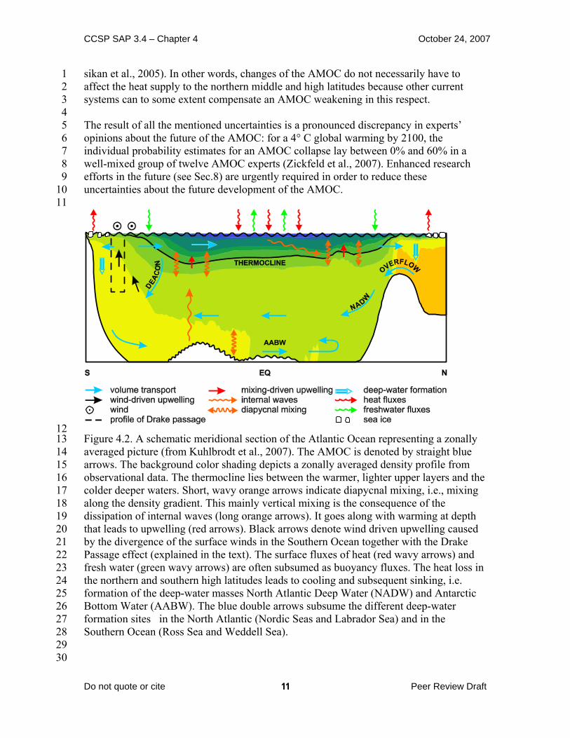
Figure 4.2. A schematic meridional section of the Atlantic Ocean representing a zonally averaged picture (from Kuhlbrodt et al., 2007). The AMOC is denoted by straight blue arrows. The background color shading depicts a zonally averaged density profile from observational data. The thermocline lies between the warmer, lighter upper layers and the colder deeper waters. Short, wavy orange arrows indicate diapycnal mixing, i.e., mixing along the density gradient. This mainly vertical mixing is the consequence of the dissipation of internal waves (long orange arrows). It goes along with warming at depth that leads to upwelling (red arrows). Black arrows denote wind driven upwelling caused by the divergence of the surface winds in the Southern Ocean together with the Drake Passage effect (explained in the text). The surface fluxes of heat (red wavy arrows) and fresh water (green wavy arrows) are often subsumed as buoyancy fluxes. The heat loss in the northern and southern high latitudes leads to cooling and subsequent sinking, i.e. formation of the deep-water masses North Atlantic Deep Water (NADW) and Antarctic Bottom Water (AABW). The blue double arrows subsume the different deep-water formation sites in the North Atlantic (Nordic Seas and Labrador Sea) and in the Southern Ocean (Ross Sea and Weddell Sea).
Do not quote or cite Peer Review Draft
11

CCSP SAP 3.4 – Chapter 4 October 24, 2007
Do not quote or cite Peer Review Draft
12
1
2 3 4 5 6 7 8 9
10 11
Figure4.3. Sketch of the two driving mechanisms, mixing (case 1) and wind-driven upwelling (case 2). The sketches are schematic pictures of meridional sections of the Atlantic. Deep water is formed at the right-hand side of the boxes and goes along with heat loss. The curved solid line separates deep dense water (ρ1) from lighter surface water (ρ2). The solid arrows indicate volume flux; the zigzag arrow denotes downward heat flux. Figure from Kuhlbrodt et al. (2007).
CCSP SAP 3.4 – Chapter 4 October 24, 2007
3 WHAT IS THE PRESENT STATE OF THE MOC? 1 2 3 4 5 6 7 8 9
10 11 12 13 14 15 16 17 18 19 20 21 22 23 24 25 26 27 28 29 30 31 32 33 34 35 36 37 38 39 40 41 42 43 44 45 46 47
The concept of a Meridional Overturning Circulation (MOC) involving sinking of cold waters in high-latitude regions and poleward return flow of warmer upper ocean waters can be traced to the early 1800s (Rumford, 1800; Humbolt, 1814). Since then, the concept has evolved into the modern paradigm of a “global ocean conveyor” connecting a small set of high-latitude sinking regions with more broadly distributed global upwelling patterns via a complex interbasin circulation (Stommel, 1958; Gordon, 1986). The general pattern of this circulation has been established for decades based on global hydrographic observations, and continues to be refined. However, measurement of the MOC remains a difficult challenge, and serious efforts toward quantifying the MOC, and monitoring its change, have developed only recently. Current efforts to quantify the MOC using ocean observations rely on four main approaches: 1. Static ocean "inverse" models utilizing multiple hydrographic sections 2. Analysis of individual transoceanic hydrographic sections 3. Continuous time-series observations along a transoceanic section, and 4. Time-dependent ocean "state estimation" models We describe, in turn, the fundamentals of these approaches and their assumptions, and the most recent results on the Atlantic MOC that have emerged from each one. In principle the MOC can also be estimated from ocean models driven by observed atmospheric forcing that are not constrained by ocean observations, or by coupled ocean-atmosphere models. There are many examples of such calculations in the literature, but we will restrict our review to those estimates that are constrained in one way or another by ocean observations. 3.1 Ocean Inverse Models Ocean "inverse" models combine several (two or more) hydrographic sections bounding a specified oceanic domain to estimate the total ocean circulation through each section. These are often referred to as "box inverse" models because they close off an oceanic "box" defined by the sections and adjacent continental boundaries, thereby allowing conservation statements to be applied to the domain. The data used in these calculations consist of profiles of temperature and salinity at a number of discrete stations distributed along the sections. The models assume a geostrophic balance for the ocean circulation (apart from the wind-driven surface Ekman layer), and derive the geostrophic velocity profile between each pair of stations, relative to an unknown reference constant, or "reference velocity." The distribution of this reference velocity along each section, and therefore the absolute circulation, is determined by specifying a number of constraints on the circulation within the box and then solving a least-squares (or other mathematical optimization) problem that best fits the constraints, within specified error tolerances. The specified constraints can be many but typically include -- above all -- overall mass conservation within the box, mass conservation within specified layers, independent observational estimates of mass transports through parts of the sections (e.g., transports
Do not quote or cite Peer Review Draft
13

CCSP SAP 3.4 – Chapter 4 October 24, 2007
1 2 3 4 5 6 7 8 9
10 11 12 13 14 15 16 17 18 19 20 21 22 23 24 25 26 27 28 29 30 31 32 33 34 35 36 37 38 39 40 41 42 43 44 45 46 47
derived from current meter arrays), and conservation of property transports (e.g., salt, nutrients, geochemical tracers). Increasingly, the solutions may also be constrained by estimates of surface heat and fresh-water fluxes. Once a solution is obtained, the transport profile through each section can be derived, and the MOC (for zonal basin-spanning sections) can be estimated. The most comprehensive and up-to-date inverse anaylses for the global time-mean ocean include those by Ganachaud (2003a) and Lumpkin and Speer (2007, Fig.4.4), based on the WOCE (World Ocean Circulation Experiment) hydrographic data collected during the 1990s. The strength of the Atlantic MOC is given as 18 ± 2.5 Sv by Lumpkin and Speer (2007) near 24ºN., where it reaches its maximum value. The corresponding estimate from Ganachaud (2003a) is 16 ± 2 Sv, in agreement within the error estimates. In both analyses the MOC strength is nearly uniform throughout the Atlantic from 20ºS. to 45ºN., ranging from approximately 14 to 18 Sv. These estimates should be taken as being representative of the average strength of the MOC over the period of the observations. An implicit assumption in these analyses is that the ocean circulation is in a "steady state" over the time period of the observations, in the above cases over a span of some 10 years. This is undoubtedly untrue, as estimates of relative geostrophic transports across individual repeated sections in the North Atlantic show typical variations of ± 6 Sv (Ganachaud, 2003a; Lavin et al., 1998). This variability is accounted for in the inverse models by allowing a relatively generous error tolerance on mass conservation, particularly in upper-ocean layers, which exhibit the strongest temporal variability. While this is an acknowledged weakness of the technique, it is offset by the large number of independent sections included in these (global) analyses, which tend to iron out deviations in individual sections from the time mean. The overall error estimates for the MOC resulting from these analyses reach about 10-15% of the MOC magnitude in the mid-latitude North Atlantic, which at the present time can probably be considered as the best constrained available estimate of the "mean" current (1990s) state of the Atlantic MOC. However, unless repeated over different time periods, these techniques are unable to provide information on the temporal variability of the MOC. 3.2 Individual Transoceanic Hydrographic Sections Historically, analysis of individual transoceanic hydrographic sections has played a prominent role in estimating the strength of the MOC and the meridional transport of heat of the oceans (Hall and Bryden, 1982). The technique is similar to that of the box inverse techniques except that only a single overall mass constraint -- the total mass transport across the section -- is applied. Other constraints, such as the transports of western boundary currents known from other direct measurements, can also be used where available. The general methodology is summarized in Box 4.1. Determination of the unknown "reference velocity" in the ocean interior is usually accomplished either by an assumption that it is uniform across the section or by adjusting it in such a way (subject to overall mass conservation) that it satisfies other a priori constraints, such as the expected flow directions of specific water masses. Variability in the reference velocity is only important to the estimation of the MOC in regions where the topography is much
Do not quote or cite Peer Review Draft
14

CCSP SAP 3.4 – Chapter 4 October 24, 2007
1 2 3 4 5 6 7 8 9
10 11 12 13 14 15 16 17 18 19 20 21 22 23 24 25 26 27 28 29 30 31 32 33 34 35 36 37 38 39 40 41 42 43 44 45 46 47
shallower than the mean depth of the section, which is normally confined to narrow continental margins where additional direct observations, if available, are included in the overall calculation. The best studied location in the North Atlantic, where this methodology has been repeatedly applied to estimate the MOC strength, is near 24ºN., where a total of five transoceanic sections have been acquired between 1957 and 2004. The MOC estimates derived from these sections range from 14.8 to 22.9 Sv, with a mean value of 18.4 ± 3.1 Sv (Bryden et al., 2005). Individual sections have an estimated error of ±6 Sv, considerably larger than the error estimates from the above inverse models. Two sections that were acquired during the WOCE period (in 1992 and 1998) yield MOC estimates of 19.4 and 16.1 Sv, respectively. Therefore these estimates are consistent with the WOCE inverse MOC estimates at 24ºN. within their quoted uncertainty, as is the mean value of all of the sections (18.4 Sv). Bryden et al. (2005) note a trend in the individual section estimates, with the largest MOC value (22.9 Sv) occurring in 1957 and weakest in 2004 (14.8 Sv) , suggesting a nearly 30% decrease in the MOC over this period (Fig. 4.5). Taken at face value, this trend is not significant, since the total change of 8 Sv between 1957 and 2004 falls within the bounds of the error estimates. However, Bryden et al. (2005) argue, based upon their finding of a consistent reduction in only the deepest layer of southward NADW flow in recent years compensating the reduced northward transport of upper ocean waters, that this change indeed likely reflects a longer term trend rather than random variability. This result remains controversial. Based upon more recent data collected within the RAPID program (see below), which better resolves the temporal variability of the interior geostrophic flow field, it is now believed that such a trend cannot be supported with the available data. A similar analysis of available hydrographic sections at 48ºN., though less well constrained by western boundary observations than at 24ºN., suggests a MOC variation there of between 9 to 19 Sv, based on three sections acquired between 1957 and 1992 (Koltermann et al., 1999). The evidence from individual hydrographic sections therefore points to regional variations in the Atlantic MOC of order 4-5 Sv, or about ±25% of its mean value. The time scales associated with this variability cannot be established from these sections, which effectively can only be considered to be "snapshots" in time. Such estimates are, therefore, potentially vulnerable to aliasing by all time scales of MOC variability. 3.3 Continuous time-series observations Until recently, there had never been an attempt to continuously measure the MOC with time-series observations covering the full width and depth of an entire transoceanic section. Motivated by the uncertainty surrounding "snapshot" MOC estimates derived from hydrographic sections, a joint U.K.-U.S. observational program, referred to as "RAPID-MOC," was mounted in 2004 to begin to continuously monitor the MOC at 26ºN. in the Atlantic. The overall strategy consists of the deployment of deep water hydrographic moorings (moorings with temperature and salinity recorders spanning the water column) on either
Do not quote or cite Peer Review Draft
15

CCSP SAP 3.4 – Chapter 4 October 24, 2007
1 2 3 4 5 6 7 8 9
10 11 12 13 14 15 16 17 18 19 20 21 22 23 24 25 26 27 28 29 30 31 32 33 34 35 36 37 38 39 40 41 42 43 44 45 46 47
side of the basin to monitor the basin-wide geostrophic shear, combined with observations from clusters of moorings on the western (Bahamas) and eastern (African) continental margins, and direct measurements of the flow though the Straits of Florida by electronic cable (see Box 4.1). Moorings are also included on the flanks of the Mid-Atlantic Ridge to resolve flows in either sub-basin. Ekman transports derived from winds (estimated from satellite measurements) are then combined with the geostrophic and direct current observations and an overall mass conservation constraint to continuously estimate the basin-wide MOC strength and vertical structure (Cunningham et al., 2007; Kanzow et al., 2007). Although only the first year of results are presently available from this program, they provide a unique new look at MOC variability (Fig. 4.6) and provide new insights on estimates derived from one-time hydrographic sections. The annual mean strength and standard deviation of the MOC, from March 2004 to March 2005, was 18.7 ± 5.6 Sv, with instantaneous (daily) values varying over a range of nearly 10-30 Sv. The Florida Current, Ekman, and mid-ocean geostrophic transport were found to contribute about equally to the variability in the upper ocean limb of the MOC. The compensating southward flow in the deep ocean (identical to the red curve in Fig. 4.6 but opposite in sign), also shows substantial changes in the vertical structure of the deep flow, including several temporary periods where the transport of lower NADW across the entire section (associated with source waters originating in the Norwegian-Greenland sea dense overflows) is nearly, or totally, interrupted. These result show that the MOC can, and does, vary substantially on relatively short time scales and that MOC estimates derived from one-time hydrographic sections are likely to be seriously aliased by short-term variability. Although the short-term variability of the MOC is large, the standard error in the 1-year RAPID estimate derived from the autocorrelation statistics of the time series is approximately 1.5 Sv (Cunningham et al., 2007). Thus, this technique should be capable of resolving interannual variability or trends of the order of 1-2 Sv. The one year (2004-05) estimate of the MOC strength of 18.7 ± 1.5 Sv is consistent, within error estimates, with the corresponding values near 26°N. determined from the WOCE inverse analysis (16-18 ± 2.5 Sv). It is also consistent with the 2004 hydrographic section estimate of 14.8 ± 6 Sv, which took place during the first month of the RAPID time series (April 2004), during a period when the MOC was weaker than its year-long average value (Fig. 4.5). 3.4 Time-varying Ocean State Estimation With recent advances in computing capabilities and global observations from both satellites and autonomous in-situ platforms, the field of oceanography is rapidly evolving toward operational applications of ocean state estimation analogous to that of atmospheric reanalysis activities. A large number of these activities are now underway that are beginning to provide first estimates of the time-evolving ocean "state" over the last 50+ years during which sufficient observations are available to constrain the models. There are two basic types of methods, (1) variational adjoint methods based on control theory, and (2) sequential estimation based on stochastic estimation theory. Both
Do not quote or cite Peer Review Draft
16

CCSP SAP 3.4 – Chapter 4 October 24, 2007
1 2 3 4 5 6 7 8 9
10 11 12 13 14 15 16 17 18 19 20 21 22 23 24 25 26 27 28 29 30 31 32 33 34 35 36 37 38 39 40 41 42 43 44 45 46
methods involve numerical ocean circulation models forced by global atmospheric fields (typically derived from atmospheric reanalyses) but differ in how the models are adjusted to fit ocean data. Sequential estimation methods use specified atmospheric forcing fields to drive the models, and progressively correct the model fields in time to fit (within error tolerances) the data as they become available (e.g., Carton et al., 2000). Adjoint methods use an iterative process to minimize differences between the model fields and available data over the entire duration of the model run (up to 50 years), through adjustment of the atmospheric forcing fields and model initial conditions, as well as internal model parameters (e.g., Wunsch, 1996). Except for the simplest of the sequential estimation techniques, both approaches are computationally expensive, and capabilities for running global models for relatively long periods of time and at a desirable level of spatial resolution are currently limited. However, in principle these models are able to extract the maximum amount of information from available ocean observations and provide an optimum, and dynamically self-consistent, estimate of the time-varying ocean circulation. Many of these models now incorporate a full suite of global observations, including satellite altimetry and sea surface temperature observations, hydrographic stations, autonomous profiling floats, subsurface temperature profiles derived from bathythermographs, surface drifters, tide stations, and moored buoys. Progress in this area is fostered by the International Climate Variability and Predictability (CLIVAR) Global Synthesis and Observations Panel (GSOP) through synthesis intercomparison and verification studies (http://www.clivar.org/organization/gsop/reference.php). A time series of the Atlantic MOC at 25ºN. derived from an ensemble average of three of these state estimation models, covering the 40-year period from 1962 to 2002, is shown in Fig. 4.5. The average MOC strength over this period is about 15 Sv, with a typical model spread of ± 3 Sv. The models suggest interannual MOC variations of 2-4 Sv with a slight increasing (though insignificant) trend over the four decades of the analysis. The mean estimate for the WOCE period (1990-2000) is 15.5 Sv, and agrees within errors with the 16-18 Sv mean MOC estimates from the foregoing WOCE inverse analyses. In comparing these results with the individual hydrographic section estimates, it is notable that only the 1998 (and presumably also the more recent 2004) estimates fall within the spread of the model values. However, owing to the large error bars on the individual section estimates, this disagreement cannot be considered statistically significant. The limited number of models presently available for these long analyses may also underestimate the model spread that will occur when more models are included. It should be noted that these models are formally capable of providing error bars on their own MOC estimates, although as yet this task has generally been beyond the available computing resources. This should become a priority once feasible. A noteworthy feature of Fig. 4.5 is the apparent increase in the MOC strength between the end of the model analysis period in 2002 and the 2004-05 RAPID estimate, an increase of some 4 Sv. The RAPID estimate lies near the top of the model spread of the preceding four decades. Whether this represents a temporary interannual increase in the MOC that will also be captured by the synthesis models when they are extended through
Do not quote or cite Peer Review Draft
17

CCSP SAP 3.4 – Chapter 4 October 24, 2007
1 2 3 4 5 6 7 8 9
10 11 12 13 14 15 16 17 18 19 20 21 22 23 24 25 26 27 28 29 30 31 32 33 34 35 36 37 38 39 40 41 42 43 44 45 46
this period, or will represent an ultimate disagreement between the estimates, awaits determination. 3.5 Conclusions and Outlook The main findings of this report concerning the present state of the Atlantic MOC can be summarized as follows: The WOCE inverse model results (e.g., Ganachaud, 2003b; Lumpkin and Speer, 2007) provide, at this time, our most robust estimates of the recent “mean state” of the MOC, in the sense that they cover an analysis period of about a decade (1990-2000) and have quantifiable (and reasonably small) uncertainties. These analyses indicate an average MOC strength in the mid-latitude North Atlantic of 16-18 Sv. Individual hydrographic sections widely spaced in time are not a viable tool for monitoring the MOC. However, these sections, especially when combined with geochemical observations, still have considerable value in documenting longer-term property changes that may accompany changes in the MOC, and in the estimation of meridional property fluxes including heat, freshwater, carbon, and nutrients. Continuous estimates of the MOC from programs such as RAPID are able to provide accurate estimates of annual MOC strength and interannual variability, with uncertainties on the annually averaged MOC of 1-2 Sv, comparable to uncertainties available from the WOCE inverse analyses. RAPID is planned to continue through at least 2014 and should provide a critical benchmark for ocean synthesis models. Time-varying ocean state estimation models are still in a development phase but are now providing first estimates of MOC variability, with encouraging agreement between different techniques. While there is still considerable research required to further refine and validate these models, including specification of uncertainties, this approach should ultimately lead to our best estimates of the large-scale ocean circulation and MOC variability. Our assessment of the state of the Atlantic MOC has been focused on 24ºN., owing to the concentration of observational estimates there, which, in turn, is historically related to the availability of long-term, high-quality western boundary current observations at this location. The extent to which MOC variability at this latitude, apart from that due to local wind-driven (Ekman) variability, is linked to other latitudes in the Atlantic remains an important research question. Also important are changes in the structure of the MOC, which could have long-term consequences for climate independent of changes in overall MOC strength. For example, changes in the relative contributions of Southern Hemisphere water masses that make up the warm return flow of the cell ( i.e., Indian Ocean thermocline water vs. Subantarctic Mode Water and Antarctic Intermediate Water) could significantly impact the temperature and salinity of the North Atlantic over time and feed back on the deep water mass formation process.
Do not quote or cite Peer Review Draft
18

CCSP SAP 3.4 – Chapter 4 October 24, 2007
1 2 3 4 5 6 7 8 9
10 11 12 13 14 15 16 17 18
Natural variability of the MOC is driven by processes acting on a wide range of time scales. On intraseasonal to intrannual time scales, the dominant processes are wind-driven Ekman variability and internal changes due to Rossby or Kelvin (boundary) waves. On interannual to decadal time scales, both variability in Labrador Sea convection related to NAO forcing and wind-driven baroclinic adjustment of the ocean circulation are implicated in models (e.g., Boning et al., 2006). Finally, on multidecadal time scales, there is growing model evidence that large-scale observed interhemispheric SST anomalies are linked to MOC variations (Knight et al., 2005; Zhang and Delworth, 2006). Our ability to detect future changes and trends in the MOC depends critically on our knowledge of the spectrum of MOC variability arising from these natural causes. The identification, and future detection, of MOC changes will ultimately rely on building a better understanding of the natural variability of the MOC on the interannual to multidecadal time scales that make up the lower frequency end of this spectrum.
19 20 21 22 23
24
25 26 27 28 29
Do not quote or cite Peer Review Draft
19

CCSP SAP 3.4 – Chapter 4 October 24, 2007
1 2 3 4 5 6 7 8 9
10
Figure 4.4. Schematic of the Atlantic MOC and major currents involved in the upper (red) and lower (blue) limbs of the MOC, after Lumpkin and Speer (2007). The boxed numbers indicate the magnitude of the MOC at several key latitudes, along with error estimates. The red to green to blue transition on various curves denotes a cooling (red is warm, blue is cold) and sinking of the water mass along its path (Figure courtesy of R. Lumpkin, NOAA/AOML.)
Do not quote or cite Peer Review Draft
20

CCSP SAP 3.4 – Chapter 4 October 24, 2007
1 2 3 4 5 6 7 8 9
10 11 12 13
Figure 4.5. Strength of the Atlantic MOC at 24ºN. derived from an ensemble average of three state estimation models (solid curve), and the model spread (shaded), for the period 1962-2002 (courtesy of the CLIVAR Global Synthesis and Observations Panel, GSOP). The estimates from individual hydrographic sections at 24ºN. (from Bryden et al., 2005), and from the 2004-05 RAPID-MOC Array (Cunningham et al., 2007) are also indicated, with respective uncertainties.
Do not quote or cite Peer Review Draft
21

CCSP SAP 3.4 – Chapter 4 October 24, 2007
1 2 3 4 5 6 7 8 9
10 11 12 13 14
Figure 4.6. Time series of MOC variability at 26ºN. ("overturning", red curve), derived from the 2004-05 RAPID Array (from Cunningham et al., 2007). Individual contributions to the total upper ocean flow across the section by the Florida Current (blue), Ekman transport (black), and the mid-ocean geostrophic flow (magenta) are also shown. A 2-month gap in the Florida current transport record during September to November 2004 was caused by hurricane damage to the electromagnetic cable monitoring station on the Bahamas side of the Straits of Florida.
Do not quote or cite Peer Review Draft
22
CCSP SAP 3.4 – Chapter 4 October 24, 2007
4 WHAT IS THE EVIDENCE FOR PAST CHANGES IN THE OVERTURNING CIRCULATION?
1 2 3 4 5 6 7 8 9
10 11 12 13 14
15 16 17 18 19 20 21 22 23 24 25 26 27 28 29 30 31 32 33 34 35 36 37 38 39 40 41 42 43
Our knowledge of the mean state and variability of the AMOC is limited by the short duration of the instrumental record. Thus, in order to gain a longer term perspective on AMOC variability and change, we turn to proxy records from past climates that can yield important insights on past climate changes, especially those that relate to the AMOC. In particular, we focus on records from the last glacial period, for which there is evidence of a rich spectrum of climate variability and change, likely linked to changes in the AMOC. Improving our ability to characterize and understand past AMOC changes will increase confidence in our ability to predict any future changes in the AMOC, as well as the global impact of these changes on the Earth’s natural systems. 4.1 Records of Abrupt Climate Change During the Last Glacial Period
The last glacial period was characterized by large, widespread and often abrupt climate changes at millennial (1,000 year) timescales. Changes in the AMOC with attendant feedbacks provide a consistent and unifying explanation for three fundamental characteristics of millennial-scale variability identified from a wide variety of highly resolved and well-dated records: (1) the amplitude of variability varies as a function of the amount of ice on the planet, with greatest amplitude being associated with intermediate ice volume (Raymo et al., 1998; McManus et al., 1999; Schulz et al., 1999; Bartoli et al., 2006), (2) in many parts of the world, this variability is characterized by abrupt switches between two preferred states, and (3) there are two spatially distinct signals, referred to as “northern” and “southern” signals in recognition of their association with the Northern and Southern Hemispheres (Alley and Clark, 1999; Clark et al., 2002, 2007). The northern signal displays the same signature and timing of climate changes as those first identified from Greenland ice-core records, wherein the so-called Dansgaard-Oeschger (D-O) oscillations are characterized by alternating warm (interstadial) and cold (stadial) states lasting for millennia, with abrupt transitions between states of up to 16oC occurring over decades or less (Johnsen et al., 1992; Grootes et al., 1993; Cuffey and Clow, 1997; Severinghaus et al., 1998; Huber et al., 2006) (Fig. 4.7a). Bond et al. (1993) recognized that several successive D-O oscillations of decreasing amplitude represented a longer term (~7,000-year) climate oscillation that culminates in a massive release of icebergs from the Laurentide Ice Sheet, known as a Heinrich event (Fig.4.7a). In contrast, the southern signal, best represented by A-events seen in Antarctic ice core records (Fig. 4.7i), exhibits less abrupt, smaller amplitude millennial changes in temperature. Synchronization of Greenland and Antarctic ice core records (Sowers and Bender, 1995; Bender et al., 1994, 1999; Blunier et al., 1998; Blunier and Brook, 2001; EPICA Community Members, 2006) demonstrates that the thermal contrast between hemispheres is greatest at the time of Heinrich events (Fig. 4.7). In the following, we elaborate on the characteristics of northern and southern signals as well as of Heinrich events. 4.1.1 The Northern Signal
Do not quote or cite Peer Review Draft
23

CCSP SAP 3.4 – Chapter 4 October 24, 2007
1 2 3 4 5 6 7 8 9
10 11 12 13 14 15 16 17 18 19 20 21 22 23 24 25 26 27 28 29 30
31 32 33 34 35 36 37 38 39 40 41 42 43 44 45
The canonical template for characterizing the northern signal comes from Greenland ice cores, in which D-O oscillations range from 1,000 to 4,000 years in duration and have a characteristic pattern of abrupt (years to decades) warming into an interstadial which is followed by a cooling interval that initially is gradual (centuries to millennia) but abruptly transitions into a cold (stadial) interval (Fig.4.7a). Although possibly influenced by moisture sources and other controls, independent constraints demonstrate that, to a first order, changes in the δ18O of Greenland ice closely parallel temperature changes (Cuffey and Clow, 1997; Severinghaus et al., 1998; Huber et al., 2006), with a large fraction of the D-O signal likely representing changes in seasonality as determined by sea-ice extent (Steig et al., 1994; Denton et al., 2005; Masson-Delmotte et al., 2005; Huber et al., 2006).
An objective characterization of modes of variability using empirical orthogonal function (EOF) analysis of several tens of high-resolution paleoclimate time series indicates that this signal is the dominant mode of variability in paleoclimate records that span a range of latitudes in the Northern Hemisphere (Clark et al., 2002, 2007). Fig. 4.7presents several of the key paleoclimate records, shown on their published chronologies, which show this broad hemispheric distribution of the D-O pattern. With regard to a stadial phase of a D-O event in Greenland, these and other records are interpreted to indicate a dustier and windier atmosphere (Mayewski et al., 1997), colder sea surface temperatures in the North Atlantic (Fig.4.7b) (Bond et al., 1993; Shackleton et al., 2000), weaker summer East Asian and Arabian monsoon systems (Fig.4.7b) (Schulz et al., 1998; Wang et al., 2001), enhanced North Pacific intermediate-water formation linked to strengthening of the Aleutian Low (Fig. 4.7d) (Hendy and Kennett, 2000), drying in the Tropics, possibly associated with a shift in the mean position of the Intertropical Convergence Zone (ITCZ) as a result of an increased pole-to-equator temperature gradient (Fig. 4.7e) (Peterson et al., 2000; Blunier and Brook, 2001; Ivanochko et al., 2005), decreased easterly atmospheric moisture transport across Central America (Peterson et al., 2000; Benway et al., 2006; Leduc et al., 2007), and enhanced sea-surface salinities in the northwestern tropical Pacific (Stott et al., 2002). 4.1.2 Heinrich Events
Heinrich (1988) first described six unusual layers of ice-rafted debris (IRD) deposited in the North Atlantic Ocean during the last glaciation that Broecker et al. (1992) subsequently named Heinrich layers 1 through 6. Later discovery of a seventh layer occurring between Heinrich layers 5 and 6 (Stoner et al., 1998, 2000; Sarnthein et al., 2001; Rashid et al., 2003) indicates temporal spacing of ~7,000 years (7 kyr) between the layers (Fig.4.7). Heinrich layers are distinguished from other IRD layers in the North Atlantic by (1) their lithologic signature indicating a dominant source from the central regions of the Laurentide Ice Sheet (Gwiazda et al., 1996; Hemming et al., 1998), (2) their increasing thickness westward toward Hudson Strait (Dowdeswell et al., 1995), and (3) their rapid sedimentation rates (McManus et al., 1998). Each layer is also associated with a large decrease in planktonic δ18O which is interpreted as a low-salinity signal derived from the melting of the icebergs (Bond et al., 1992; Hillaire-Marcel and Bilodeau, 2000; Roche et al., 2004). Recent estimates suggest that the duration of Heinrich layers was on order of 500 years(Hemming, 2004; Roche et al., 2004). These characteristics are consistent with the hypothesis of Broecker et al. (1992) that Heinrich
Do not quote or cite Peer Review Draft
24

CCSP SAP 3.4 – Chapter 4 October 24, 2007
1 2 3 4 5 6 7 8 9
10 11 12 13 14 15 16 17 18 19 20 21 22 23 24 25
26 27 28 29 30 31 32 33 34 35 36 37 38 39 40 41 42 43 44 45
layers represent a massive flux of icebergs which were rapidly released into the North Atlantic Ocean in association with a surge from the Laurentide Ice Sheet (e.g., Heinrich events) (Marshall and Koutnik, 2006). Less clear, however, is the amount of sea level change associated with Heinrich events. Model results and δ18O anomalies of North Atlantic surface-water suggest sea-level changes were likely <3 meters (m) (MacAyeal, 1993; Marshall and Clarke, 1997; Roche et al., 2004). Several mechanisms have been proposed for the cause of Heinrich events, including internal ice-sheet dynamics (MacAyeal, 1993; Calov et al., 2002) or an external trigger (Hulbe et al., 2004; Shaffer et al., 2004; Fluckiger et al., 2006; Clark et al., 2007), but no consensus hypothesis has yet emerged. This remains a critical question, however, with regard to understanding the role of Heinrich events in causing changes in the AMOC. A number of paleoclimate records suggest that during Heinrich events, the hydrological cycle was enhanced over currently arid northeastern Brazil (Arz et al., 1998; Wang et al., 2004) and Florida (Grimm et al., 2006), while northeastern Africa became drier (Ivanochko et al., 2005). In addition, surface-water productivity increased in the subpolar Southern Ocean (Fig. 4.7f) (Sachs and Anderson, 2005). Several records exhibiting D-O- and Heinrich-like variability show that cooling in the North Atlantic and Mediterranean (Fig. 4.7b) (Cacho et al., 1999; Shackleton et al., 2000; Pailler and Bard, 2002), attenuation of the water balance in northern South America (Peterson et al., 2000), and suppression of Arabian and East Asian monsoons (Fig. 4.7c) (Schulz et al., 1998; Wang et al., 2001) all were greatest at times of Heinrich events. Other records with D-O-like variability, including Greenland δ18O records (Fig. 4.7a), do not indicate any greater response during Heinrich events than the responses recorded during intervening stadials or their equivalents. 4.1.3 Southern Signal
The canonical template for this mode of variability is the millennial-scale signal in Antarctic ice cores represented by A events (Fig. 4.7i). These events differ from most D-O events in that they are of longer duration (~4-5 kyr) and display a more symmetrical shape of gradual warming and cooling. The A events are the largest amplitude millennial-scale signal in Antarctic ice cores between 20 and 65 thousand years before present (ka). Correlation of Antarctic and Greenland ice core records using methane records indicates that A events are not in phase with the longest D-O events (Fig.4.7) (Blunier et al., 1998; Blunier and Brook, 2001). Antarctic warming began during a Greenland stadial and continued until the abrupt onset of a Greenland interstadial. At that time, temperatures in both regions decreased but more rapidly in Antarctica than in Greenland. Based on correlation using the δ18O of molecular O2 of air in ice cores, Bender et al. (1999) proposed that the smaller Antarctic events are similarly correlative with the shorter D-O events. Recent methane correlation between the North Greenland Ice core Project (NGRIP) ice core and the EPICA Dronning Maud Land (EDML) ice core supports this proposal (EPICA Community Members, 2006), but whether these shorter events are correlative from one region of Antarctica to another has yet to be established. EOF analysis indicates that this signal is the dominant mode of variability in paleoclimate records that span a range of latitudes in the Southern Hemisphere (Clark et al., 2002, 2007). The presence of the A events in five widely distributed Antarctic ice cores indicates a coherent pattern over the continent. Changes in SSTs in the southwest
Do not quote or cite Peer Review Draft
25

CCSP SAP 3.4 – Chapter 4 October 24, 2007
Pacific (Fig. 4.7g) (Pahnke et al., 2003), the southeast Pacific (Kaiser et al., 2005), and the South Atlantic (Charles et al., 1996; Ninneman et al., 1999) are all thought to be correlative to A events, suggesting a Southern Ocean response that extends at least to the mid-latitudes. Robinson et al. (2007) interpret increases in δ15N from the southeast Pacific as an increased nutrient supply from the Southern Ocean induced by partial breakdown of stratification during A-event warmings. Finally, changes in atmospheric CO2 of ~20 parts per million by volume (ppmV) co-varied with A events with a time lag of 720
1 2 3 4 5 6 7
+370 yr (Fig. 4.7h) (Indermuhle et al., 2000; Ahn and Brook, 2007). 8 9
10
11 12 13 14 15 16 17 18 19 20 21 22 23 24 25 26 27 28 29 30 31 32 33 34 35 36 37 38 39 40 41 42 43 44
4.2 Evidence for Past Changes in the AMOC and Their Relation to Climate Change
Models and data have suggested that millennial-scale climate variability during the last glacial period (Fig. 4.7) was associated with three modes of the AMOC: (1) an interstadial mode similar to the modern AMOC, (2) a stadial mode associated with a southward shift in sites of North Atlantic Deepwater (NADW) formation, possibly with a shoaling of the depth of its formation such as characterized the Last Glacial Maximum (LGM) 21,000 years ago, and (3) a Heinrich mode in which the AMOC was effectively shut down (Sarnthein et al., 1994, 2001; Alley and Clark, 1999; Ganopolski and Rahmstorf, 2001). The climatic impacts of transitions between the first two modes were transmitted largely through the atmosphere and are thought to explain the D-O oscillations. For example, model simulations suggest that atmospheric responses to a reduced AMOC include weakening of the Indian and Asian monsoons (Timmermann et al., 2005b; Zhang and Delworth, 2005), strengthening of the Aleutian Low (Mikolajewicz et al., 1997; Zhang and Delworth, 2005), and southward migration of the position of the ITCZ (Schiller et al., 1997; Rind et al., 2001; Chiang et al., 2003; Zhang and Delworth, 2005).
The impacts of a (near) collapse of the AMOC, on the other hand, were transmitted through the ocean as well as the atmosphere. Corresponding changes in cross-equatorial heat transport establish a so-called bipolar seesaw (Mix et al., 1986; Manabe and Stouffer, 1988; Crowley, 1992; Vellinga and Wood, 2002; Zhang and Delworth, 2005) which is characterized by opposite responses in the North and South Atlantic that are amplified by corresponding changes in sea-ice extent. Southward propagation of the signal is delayed several hundred years by thermal and dynamical effects of the Antarctic Circumpolar Current (ACC) (Schmittner et al., 2003) and by the thermal reservoir of the Southern Ocean (Stocker and Johnsen, 2003). The southern signal is otherwise rapidly transmitted throughout the Southern Ocean by the ACC (Vellinga and Wood, 2002).
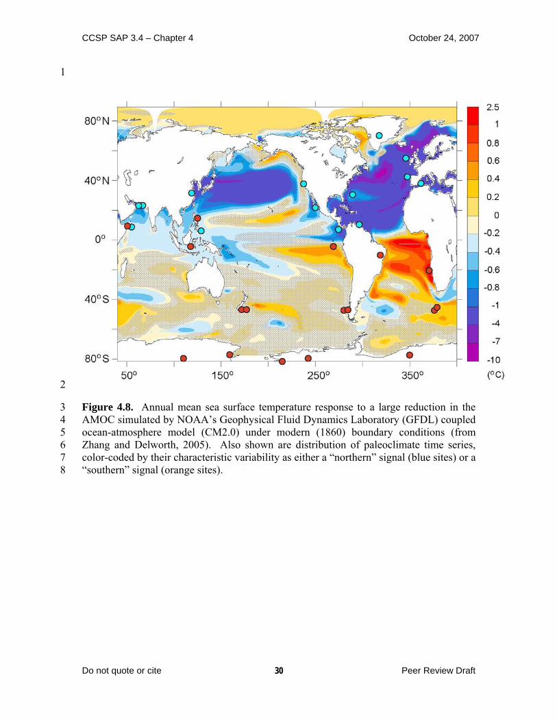
In general, the spatial distribution of climate anomalies suggested by the paleoclimate records summarized in the preceding sections is in good agreement with recent climate model simulations of a collapse of the AMOC (Fig.4.8), indicating that changes in the AMOC and attendant feedbacks can explain a substantial fraction of the millennial-scale climate variability during the last glacial period. One important region where there is disagreement is in the western tropical Pacific Ocean, where some records indicate a different response than simulated by model simulations. Some of this disagreement may reflect chronological uncertainties (Clark et al., 2007). Because of the
Do not quote or cite Peer Review Draft
26

CCSP SAP 3.4 – Chapter 4 October 24, 2007
1 2 3 4 5 6 7 8 9
10 11 12 13 14 15 16 17 18 19 20 21 22 23 24 25 26 27 28 29 30 31 32 33 34 35 36 37 38 39 40 41 42 43 44 45 46
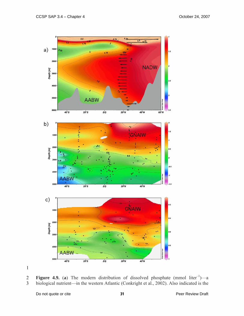
significance of this region to global climate, resolving this issue remains an important objective. Although the interval corresponding to the Last Glacial Maximum (23,000 to 19,000 years ago) does not correspond to an abrupt climate change, a large body of evidence points to a significantly different AMOC at that time (Lynch-Stieglitz et al., 2007) that was likely representative of the AMOC during other intervals of the last glacial period. The geographic distribution of different species of planktonic organisms indicates that while warm currents extend far into the North Atlantic today, compensating the export of deep waters from the polar seas, during the LGM the North Atlantic was marked by a strong east-west trending polar front separating the warm subtropical waters from the cold waters which dominated the North Atlantic during glacial times (CLIMAP, 1981; Ruddiman and McIntyre, 1981; Paul and Schafer-Neth, 2003; Kucera et al., 2005). The chemical and isotopic compositions of benthic organisms suggest that while low-nutrient North Atlantic Deep Water (NADW) dominates the deep Atlantic in the modern North Atlantic, during the LGM the deep-water masses below 2 km depth appear to be older (Keigwin, 2004) and more nutrient rich (Duplessy et al., 1988; Sarnthein et al., 1994; Bickert and Mackensen, 2004; Curry and Oppo, 2005; Marchitto and Broecker, 2006) than the waters above 2 km (Fig.4.9). Reconstructions of seawater density based on the isotopic composition of benthic shells suggests a reduced density contrast across the South Atlantic basin, implying a weakened AMOC in the upper 2 km of the South Atlantic (Lynch-Stieglitz et al., 2006), whereas the accumulation of the decay products of uranium in ocean sediments suggests that the overall residence time of deep waters in the Atlantic was only slightly longer than today (Yu et al., 1996; McManus et al., 2004). These data point to an AMOC that was probably quite different in its extent and structure from today’s, likely producing differences in the oceanic heat transport in the Atlantic during the LGM.
The most widely used proxy of millennial-scale changes in the AMOC is δ13C of dissolved inorganic carbon, which differentiates the location, depth, and volume of nutrient-depleted NADW relative to underlying nutrient-enriched Antarctic Bottom Water (AABW) (Fig.4.9) (Boyle and Keigwin, 1982; Curry and Lohman, 1982; Duplessy et al., 1988). Millennial-scale water mass variability is also seen in the distribution of other nutrient tracers (Boyle and Keigwin, 1982; Marchitto et al., 1998) and radiocarbon (Keigwin and Schlegel, 2002; Robinson et al., 2005) during the deglaciation (Younger Dryas) and possibly in Nd isotopes over at least some of the D-O events (Rutberg et al., 2000; Piotrowski et al., 2005). However, rates of flow cannot be inferred from these water mass proxies alone. Thus far, additional proxies that constrain changes in the rate of the AMOC only extend back to ~20,000 years, but they generally support the inference from δ13C that changes in depth and volume of NADW do reflect changes in the rate of the AMOC, at least for this time interval (Lynch-Stieglitz et al., 1999; McManus et al., 2004; Lynch-Stieglitz et al., 2006; McCave and Hall, 2006).
Fig. 4.10 illustrates a depth transect of δ13C records from the eastern North Atlantic that represent changes in the depth and volume (but not rate) of the AMOC during an interval (35-48 ka) of pronounced millennial-scale climate variability (Fig.4.7). The Heinrich mode of the AMOC is readily distinguished from other times by a large reduction in δ13C during Heinrich events, indicating the near-complete replacement of nutrient-poor, high δ13C NADW with nutrient-rich, low δ13C AABW in this part of the
Do not quote or cite Peer Review Draft
27

CCSP SAP 3.4 – Chapter 4 October 24, 2007
1 2 3 4 5 6 7 8 9
10 11 12 13 14 15 16 17 18 19 20 21 22 23 24 25 26 27 28 29
Atlantic basin (Fig. 4.10b). The inference of a much reduced rate of NADW formation for at least event H1 is supported by the Pa/Th ratios in the North Atlantic that approach the ratio in which they are produced in the water column (McManus et al., 2004; Gherardi et al., 2005). The observational constraints provided by the paleoclimate records support model simulations (Fig.4.8) in showing that the times of a collapsed AMOC (Fig. 4.10b) correspond to the maximum temperature differential between the two polar hemispheres (Fig. 4.10a, c).
On the other hand, the δ13C records make no clear distinction between interstadials and non-Heinrich stadials (Fig. 4.10b) (Boyle, 2000; Shackleton et al., 2000; Elliot et al., 2002). This result contrasts with changes in the relative amount of magnetic minerals in deep-sea sediments derived from Tertiary basaltic provinces underlying the Norwegian Sea, which are interpreted to record an increase (decrease) in the velocity of the overflows from the Nordic Seas during D-O interstadials (stadials) (Kissel et al., 1999). Taken at face value, the δ13C and magnetic records may indicate that latitudinal shifts in the AMOC occurred, but with little commensurate change in the depth of deep-water formation. The corresponding changes in the relative amount of magnetic minerals then reflect times when NADW formation occurred either in the Norwegian Sea, thus entraining magnetic minerals from the seafloor there, or in the open North Atlantic, at sites to the south of the source of the magnetic minerals. What remains unclear is whether changes in the overall strength of the AMOC accompanied these latitudinal shifts in NADW formation. However, the sea-ice feedbacks that would have accompanied the latitudinal shift in deep-water formation (Denton et al., 2005; Li et al., 2005; Masson-Delmotte et al., 2005) may then have been important in amplifying D-O oscillations, including far-field responses (Barnett et al., 1989; Douville and Royer, 1996; Chiang et al., 2003).
Do not quote or cite Peer Review Draft
28

CCSP SAP 3.4 – Chapter 4 October 24, 2007
1 2 3 4 5 6 7 8 9
10 11 12 13 14 15 16 17
Figure 4.7. Climate records on their published timescales showing characteristics of millennial-scale climate change discussed in the text. Vertical gray bars represent times of Heinrich events. (a) The GISP2 δ18O record (Grootes et al., 1993; Stuiver and Grootes, 2000). The slanted red lines represent the longer-term cooling trend followed by an abrupt warming, commonly referred to as Bond cycles. ‰, per mil. (b) The δ18O planktonic record from core MD95-2042 in the eastern North Atlantic (Shackleton et al., 2000). (c) Total organic carbon from Arabian Sea sediments (Schulz et al., 1998). (d) Ratio of the planktonic foraminifera N. pachyderma (Hendy and Kennett, 2000). (e) Methane record from the GISP2 ice core (Blunier and Brook, 2001). (f) Alkenone concentrations in marine sediments from southwestern Pacific Ocean (Sachs and Anderson, 2005). (g) Sea surface temperature (SST) record from the southwestern Pacific Ocean (Pahnke et al., 2003). (h) The Taylor Dome (light blue circles) (Indermuhle et al., 2000) and Bryd (dark blue circles) CO2 records, placed on the GISP2 timescale through synchronization with methane (Ahn and Brook, 2007). (i) The Byrd δ18O record (Johnsen et al., 1972), with the timescale synchronized to the GISP2 timescale by methane correlation (Blunier and Brook, 2001). ka, thousand years.
Do not quote or cite Peer Review Draft
29
CCSP SAP 3.4 – Chapter 4 October 24, 2007
1
2
3 4 5 6 7 8
Figure 4.8. Annual mean sea surface temperature response to a large reduction in the AMOC simulated by NOAA’s Geophysical Fluid Dynamics Laboratory (GFDL) coupled ocean-atmosphere model (CM2.0) under modern (1860) boundary conditions (from Zhang and Delworth, 2005). Also shown are distribution of paleoclimate time series, color-coded by their characteristic variability as either a “northern” signal (blue sites) or a “southern” signal (orange sites).
Do not quote or cite Peer Review Draft
30
CCSP SAP 3.4 – Chapter 4 October 24, 2007
1
2 3
Figure 4.9. (a) The modern distribution of dissolved phosphate (mmol liter–1)—a biological nutrient—in the western Atlantic (Conkright et al., 2002). Also indicated is the
Do not quote or cite Peer Review Draft
31

CCSP SAP 3.4 – Chapter 4 October 24, 2007
1 2 3 4 5 6 7 8 9
10 11
southward flow of North Atlantic Deep Water (NADW), which is compensated by the northward flow of warmer waters above 1 km, and the Antarctic Bottom Water (AABW) below. (b) The distribution of the carbon isotopic composition (13C/12C, expressed as δ13C, Vienna Pee Dee belemnite standard) of the shells of benthic foraminifera in the western and central Atlantic during the Last Glacial Maximum (LGM) (Bickert and Mackinson, 2004; Curry and Oppo, 2005). Data from different longitudes are collapsed in the same meridional plane. GNAIW, glacial North Atlantic intermediate water. (c) Estimates of the Cd (nmol kg–1) concentration for LGM from the ratio of Cd/Ca in the shells of benthic foraminifera, from Marchitto and Broecker (2006). Today, the isotopic composition of dissolved inorganic carbon and the concentration of dissolved Cd in seawater both show “nutrient”-type distributions similar to that of PO4.
Do not quote or cite Peer Review Draft
32

CCSP SAP 3.4 – Chapter 4 October 24, 2007
Figure4.10. (a) The GISP2 δ18O record (Grootes et al., 1993; Stuiver and Grootes, 2000). Times of Heinrich events 4 and 5 identified (H4 and H5). (b) Time-varying δ13C, a proxy for distribution of deep-water masses, as a function of depth in the eastern North
1 2 3 4
Do not quote or cite Peer Review Draft
33

CCSP SAP 3.4 – Chapter 4 October 24, 2007
Atlantic based on four δ13C records at water depths of 1,099 m (Zahn et al., 1997), 2,161 m (Elliot et al., 2002), 2,637 m (Skinner and Elderfield, 2007), and 3,146 m (Shackleton et al., 2000). Control points from four cores used for interpolation are shown (black dots). More negative δ13C values correspond to nutrient-rich Antarctic Bottom Water (AABW), whereas more positive δ13C values correspond to nutrient-poor North Atlantic Deep Water (see Fig.4.8). Also shown by the thick gray line is a proxy for Heinrich events, with peak values corresponding to Heinrich events H5 and H4 (Stoner et al., 2000) (note that scale for this proxy is not shown). During Heinrich events H5 and H4, nutrient-rich AABW displaces NADW to shallow depths in the eastern North Atlantic Basin. (c) The Byrd δ18O record (Johnsen et al., 1972), with the timescale synchronized to the GISP2 timescale by methane correlation (Blunier and Brook, 2001). ka, thousand years.
1 2 3 4 5 6 7 8 9
10 11 12 13
Do not quote or cite Peer Review Draft
34

CCSP SAP 3.4 – Chapter 4 October 24, 2007
1
2 3 4 5 6 7 8 9
10 11 12 13 14 15 16 17 18 19 20 21 22 23 24 25 26 27 28 29 30 31 32 33 34 35 36 37 38 39 40 41 42 43 44 45
5 HOW WELL DO THE CURRENT COUPLED OCEAN-ATMOSPHERE MODELS SIMULATE THE OVERTURNING CIRCULATION? Coupled ocean-atmosphere models are commonly used to make projections of how the MOC might change in future decades. Confidence in these models can be improved by making comparisons of the MOC both between models and between models and observational data. Even though the scarcity of observations presents a major challenge, it is apparent that significant mismatches are present and that continued efforts are needed to improve the skill of coupled models. This section reviews simulations of the present-day (Section 5.1), Last Glacial Maximum (Section 5.2), and transient events of the past (Section 5.3).
5.1 Present-day simulations A common model-model and model-data comparison uses the mean strength of the MOC. Observational estimates are derived from either hydrographic data (section 3.3.1; Ganachaud, 2003a; Talley et al., 2003; Lumpkin and Speer, 2007) or inventories of chlorofluorocarbon tracers in the ocean (Smethie and Fine, 2001). The estimates are consistent with each other and suggest a mean overturning of about 15-18 Sv with errors of about 2-5 Sv. In contrast, coupled atmosphere-ocean models using modern boundary conditions yield a wide range of values for overturning strength, which is usually defined as the maximum meridional overturning streamfunction value in the North Atlantic excluding the surface circulation. Present-day control (i.e., fixed forcing) simulations yield average MOC intensities from model to model between 12 and 26 Sv (Fig. 4.11; Stouffer et al., 2006), while simulations of the 20th century that include historical variations in forcing have a range from 10 to 30 Sv (Randall et al., 2007; see also Fig. 4.17). In addition, some of the 20th century simulations show substantial drifts that might hinder predictions of future MOC strength (Randall et al., 2007). There are also substantial differences among models in MOC variability, which tends to scale with the mean strength of the overturning. Models with a more vigorous overturning tend to produce pronounced multidecadal variations, while variability in models with a weaker MOC is more damped (Stouffer et al., 2006). Time series of the MOC are too incomplete to give an indication of which mode is more accurate, although recent observations suggest that the MOC is highly variable on subannual time scales (Section 3.3; Cunningham et al., 2007). Another useful model-data comparison can be made for ocean heat transport in the Atlantic. A significant fraction of the northward heat transport in the Atlantic is due to
Do not quote or cite Peer Review Draft
35

CCSP SAP 3.4 – Chapter 4 October 24, 2007
1 2 3 4 5 6 7 8 9
10 11 12 13 14 15 16 17 18 19 20 21 22 23 24 25 26 27 28 29 30 31 32 33 34 35 36 37 38 39 40 41 42 43 44 45 46
the MOC, with additional contributions from horizontal circulations (e.g., Roemmich and Wunsch, 1985). Since heat storage in the ocean is small in the long-term average and ocean heat transport must balance surface heat fluxes, the heat transport also provides an indication of how well surface fluxes are simulated. There are several calculations of heat transport at 20-25° N. in the Atlantic derived by combining hydrographic observations in inverse models. These methods yield estimates of about 1.3 Petawatts (PW; 1 PW = 1015 Watts) with errors on the order of about 0.2 PW (Ganachaud and Wunsch, 2000; Stammer et al., 2003). While all models agree that heat transport in the Atlantic is northward at 20°N., the modeled magnitude varies greatly (Fig. 4.12). Most models tend to underestimate the ocean heat transport, with ranges generally between 0.5 to 1.1 PW (Jia, 2003; Stouffer et al., 2006). The mismatch is believed to result from two factors: (1) smaller than observed temperature differences between the upper and lower branches of the MOC, with surface waters too cold and deep waters too warm, and (2) overturning that is too weak (Jia, 2003). The source of these model errors will be discussed further. Schmittner et al. (2005) and Schneider et al. (2007) have proposed that the skill of a model in producing the climatological spatial patterns of temperature, salinity and pycnocline depth in the North Atlantic is another useful measure of model ability to simulate the overturning circulation. These authors found that models constrain temperature better than salinity; they attribute errors in the latter to biases in the hydrologic cycle in the atmosphere (Schneider et al., 2007). Large errors in pycnocline depth are probably the result of compounded errors from both temperature and salinity fields. Also, errors over the North Atlantic alone tend to be significantly larger than those for the global field (Schneider et al., 2007). Large cold biases of up to several degrees Celsius in the North Atlantic, seen in most coupled models, are attributed partly to misplacement of the North Atlantic Current and the large SST gradients associated with it (Randall et al., 2007). Cold surface biases commonly contrast with temperatures that are about 2° C too warm at depth in the region of North Atlantic Deep Water (Randall et al., 2007). Some of these model errors, particularly in temperature and heat transport, are related to the representation of western boundary currents (Gulf Stream and North Atlantic Current) and deep-water overflow across the Greenland-Iceland-Scotland ridge. Two common model biases in the western boundary current are (1) a separation of the Gulf Stream from the coast of North America that occurs too far north of Cape Hatteras (Dengg et al., 1996) and (2) a North Atlantic Current whose path does not penetrate the southern Labrador Sea, and is instead too zonal with too few meanders (Rossby, 1996). The effect of the first bias is to prohibit northward meanders and warm core eddies, negatively affecting heat transport and water mass transformation, while the second bias results in SSTs that are too cold. Both of these biases have been improved in standalone ocean models by increasing the resolution to about 0.1° so that mesoscale eddies may be resolved (e.g., Smith et al., 2000; Bryan et al., 2007). The resolution of current coupled ocean-atmosphere models is typically on the order of 1° or more, requiring an increase in computing power of an order of magnitude before coupled eddy-resolving simulations become feasible. Initial results from coupling a high-resolution ocean model to an
Do not quote or cite Peer Review Draft
36

CCSP SAP 3.4 – Chapter 4 October 24, 2007
1 2 3 4 5 6 7 8 9
10 11 12 13 14 15 16 17 18 19 20 21 22 23 24 25 26 27 28 29 30 31 32 33 34 35 36 37 38 39 40 41 42 43 44 45 46
atmospheric model indicate that a corresponding increase in atmospheric resolution may also be necessary (Roberts et al., 2004). Ocean model resolution is also one of the issues involved in the representation of deep-water overflows. Deep-water masses in the North Atlantic are formed in marginal seas and enter the open ocean through overflows such as the Denmark Strait and the Faroe Bank Channel. Model simulations of overflows are unrealistic in several aspects, including (1) the specification of sill bathymetry, which is made difficult because the resolution is often too coarse to represent the proper widths and depths (Roberts and Wood, 1997), and (2) the representation of mixing of dense overflow waters with ambient waters downstream of the sill (Winton et al., 1998). In many ocean models, topography is specified as discrete levels, which leads to a “stepped” profile descending from sills. Mixing of overflow waters with ambient waters occurs at each step, leading to excessive entrainment. As a result, deep waters in the lower branch of the MOC are too warm and too fresh (e.g., Tang and Roberts, 2005). Efforts are being made to improve this model deficiency through new parameterizations (Thorpe et al., 2004; Tang and Roberts, 2005) or by using isopycnal or terrain-following vertical coordinate systems (Willebrand et al., 2001). 5.2 Last Glacial Maximum simulations Characteristics of the overturning circulation at the LGM were reviewed in Section 3. Those that are the most robust and, therefore, the most useful for evaluating model performance are (1) a shallower boundary, at a level of about 2,000-2,500 m, between Glacial North Atlantic Intermediate Water and Antarctic Bottom Water (Duplessy et al., 1988; Boyle, 1992; Curry and Oppo, 2005; Marchitto and Broecker, 2006); (2) a reverse in the north-south salinity gradient in the deep ocean to the Southern Ocean being much saltier than the North Atlantic (Adkins et al., 2002); and (3) formation of Glacial North Atlantic Intermediate Water south of Iceland (Duplessy et al., 1988; Sarnthein et al., 1994; Pflaumann et al., 2003).
It is more difficult to compare model results to inferred flow speeds, due to the lack of agreement among proxy records for this variable. Some studies suggest a vigorous circulation with transports not too different from today (McCave et al., 1995; Yu et al., 1996), while others suggest a decreased flow speed (Lynch-Stieglitz et al., 1999; McManus et al., 2004). All that can be said confidently is that there is no evidence for a significant strengthening of the overturning circulation at the LGM.
Results from LGM simulations are strongly dependent on the specified boundary conditions. In order to facilitate model-model and model-data comparisons, the second phase of the Paleoclimate Modeling Intercomparison Project (PMIP2; Braconnot et al., 2007) coordinated a suite of coupled atmosphere-ocean model experiments using common boundary conditions. Models involved in this project include both general circulation models (GCMs) and earth system models of intermediate complexity (EMICs). LGM boundary conditions are known with varying degrees of certainty. Some
Do not quote or cite Peer Review Draft
37

CCSP SAP 3.4 – Chapter 4 October 24, 2007
1 2 3 4 5 6 7 8 9
10 11 12 13 14 15 16 17 18 19 20 21 22 23 24 25 26 27 28 29 30 31 32 33 34 35 36 37 38 39 40 41 42 43 44 45 46
are known well, including past insolation, atmospheric concentrations of greenhouse gases, and sea level. Others are less certain, including the topography of the ice sheets, vegetation and other land-surface characteristics, and changes in river drainage basins. For these, PMIP2 simulations used best estimates (see Braconnot et al., 2007). More work is necessary to narrow the uncertainty of these boundary conditions, particularly since some could have important effects on the MOC.
The resulting MOC in the PMIP2 simulations for LGM boundary conditions varies widely between the models, and several of the simulations are clearly not in agreement with the paleodata (Fig. 4.13, Fig. 4.7). A shoaling of the circulation is clear in only one of the models; all other models show either a deepening or little change (Weber et al., 2007; Otto-Bliesner et al., 2007). Also, the north-south salinity gradient of the LGM deep ocean is not consistently reversed in these model simulations (Otto-Bliesner et al., 2007). All models do show a southward shift of GNAIW formation, however. In general, the better the model matches one of these criteria, the better it matches the others as well (Weber et al., 2007).
There is a particularly large spread among the models in terms of overturning strength (Fig. 4.13). Some models show a significantly increased MOC streamfunction for the LGM compared to the modern control (by ~25-40%). Others have a significantly decreased streamfunction (by ~20-30%), while another shows very little change (Weber et al., 2007). Again, the overturning strength is not constrained well enough from the paleodata to make this a rigorous test of the models. It is likely, though, that simulations with a significantly strengthened MOC are not realistic.
Several factors control the MOC response to LGM boundary conditions. These include changes in the fresh-water budget of the North Atlantic, the density gradient between the North and South Atlantic, and the density gradient between GNAIW and AABW (Schmittner et al., 2002; Weber et al. 2007). The density gradient between GNAIW and AABW appears to be particularly important, and sea ice concentrations have been shown to play a central role in determining this gradient (Otto-Bliesner et al., 2007). The MOC response also has some dependence on the accuracy of the control state. For example, models with an unrealistically shallow overturning circulation in the control simulation do not yield a shoaled circulation for LGM conditions (Weber et al., 2007).
5.3 Transient simulations of past MOC variability At various times in the past, particularly during the last glacial and deglacial periods, fresh-water input to the North Atlantic from ice sheets and glacial lakes slowed the MOC. These events offer another potential test of model skill in which the known fresh-water forcing is prescribed and the response is compared to paleodata. One of the more promising candidates for such a test is the so-called 8.2 ka event, a period of climate anomalies 8,200 years ago that occurred somewhat after the draining of a glacial lake into the Hudson Bay. This event is of particular interest because it occurred during an interglacial period and has an identified cause (Schmidt and LeGrande, 2005).
Do not quote or cite Peer Review Draft
38

CCSP SAP 3.4 – Chapter 4 October 24, 2007
1 2 3
Research on this and other events has been limited, however, because of the detailed information needed about the fresh-water fluxes (Meissner and Clark, 2006) and because quantitative reconstructions of changes in the MOC are largely lacking.
Do not quote or cite Peer Review Draft
39

CCSP SAP 3.4 – Chapter 4 October 24, 2007
1
2 3 4 5 6 7 8
Figure 4.11. Time series of the strength of the Atlantic meridional overturning as simulated by a suite of coupled ocean-atmosphere models using present-day boundary conditions, from Stouffer et al. (2006). The strength is listed along the y-axis in Sverdrups (Sv; 1 Sv = 106 m3s-1). Curves were smoothed with a 10-yr running mean to reduce high-frequency fluctuations. The numbers after the model names indicate the long-term mean of the Atlantic MOC.
Do not quote or cite Peer Review Draft
40

CCSP SAP 3.4 – Chapter 4 October 24, 2007
1
2 3 4 5 6 7 8 9
Figure 4.12. Northward heat transport in the Atlantic Ocean in an ensemble of coupled ocean-atmosphere models, from Stouffer et al. (2006). For comparison, observational estimates at 20-25°N. are about 1.3 ± 0.2 Petawatts (PW; one PW = 1015 Watts) ( (Ganachaud and Wunsch, 2000; Stammer et al., 2003).
Do not quote or cite Peer Review Draft
41

CCSP SAP 3.4 – Chapter 4 October 24, 2007
1
2 3 4 5 6 7 8 9
Figure 4.13. Atlantic meridional overturning (in Sverdrups) simulated by four PMIP2 coupled ocean-atmosphere models for modern (top) and the Last Glacial Maximum (bottom). From Otto-Bliesner et al. (2007).
Do not quote or cite Peer Review Draft
42
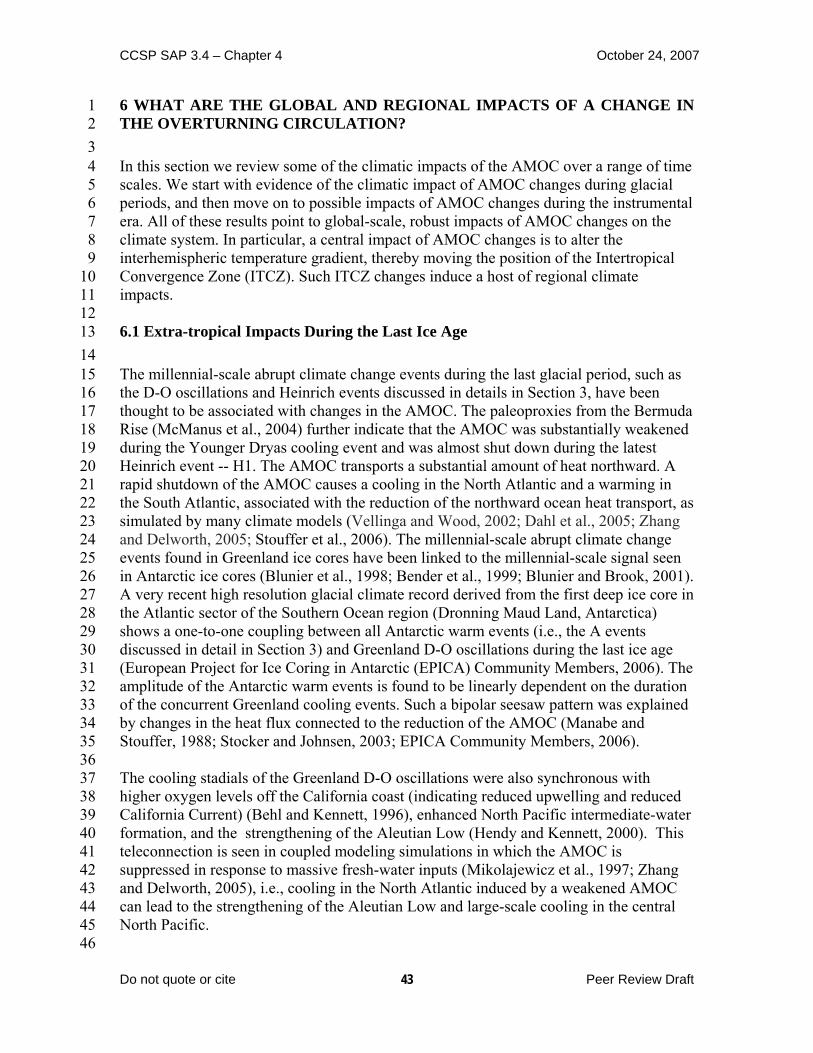
CCSP SAP 3.4 – Chapter 4 October 24, 2007
6 WHAT ARE THE GLOBAL AND REGIONAL IMPACTS OF A CHANGE IN THE OVERTURNING CIRCULATION?
1 2 3 4 5 6 7 8 9
10 11 12 13 14 15 16 17 18 19 20 21 22 23 24 25 26 27 28 29 30 31 32 33 34 35 36 37 38 39 40 41 42 43 44 45 46
In this section we review some of the climatic impacts of the AMOC over a range of time scales. We start with evidence of the climatic impact of AMOC changes during glacial periods, and then move on to possible impacts of AMOC changes during the instrumental era. All of these results point to global-scale, robust impacts of AMOC changes on the climate system. In particular, a central impact of AMOC changes is to alter the interhemispheric temperature gradient, thereby moving the position of the Intertropical Convergence Zone (ITCZ). Such ITCZ changes induce a host of regional climate impacts. 6.1 Extra-tropical Impacts During the Last Ice Age The millennial-scale abrupt climate change events during the last glacial period, such as the D-O oscillations and Heinrich events discussed in details in Section 3, have been thought to be associated with changes in the AMOC. The paleoproxies from the Bermuda Rise (McManus et al., 2004) further indicate that the AMOC was substantially weakened during the Younger Dryas cooling event and was almost shut down during the latest Heinrich event -- H1. The AMOC transports a substantial amount of heat northward. A rapid shutdown of the AMOC causes a cooling in the North Atlantic and a warming in the South Atlantic, associated with the reduction of the northward ocean heat transport, as simulated by many climate models (Vellinga and Wood, 2002; Dahl et al., 2005; Zhang and Delworth, 2005; Stouffer et al., 2006). The millennial-scale abrupt climate change events found in Greenland ice cores have been linked to the millennial-scale signal seen in Antarctic ice cores (Blunier et al., 1998; Bender et al., 1999; Blunier and Brook, 2001). A very recent high resolution glacial climate record derived from the first deep ice core in the Atlantic sector of the Southern Ocean region (Dronning Maud Land, Antarctica) shows a one-to-one coupling between all Antarctic warm events (i.e., the A events discussed in detail in Section 3) and Greenland D-O oscillations during the last ice age (European Project for Ice Coring in Antarctic (EPICA) Community Members, 2006). The amplitude of the Antarctic warm events is found to be linearly dependent on the duration of the concurrent Greenland cooling events. Such a bipolar seesaw pattern was explained by changes in the heat flux connected to the reduction of the AMOC (Manabe and Stouffer, 1988; Stocker and Johnsen, 2003; EPICA Community Members, 2006). The cooling stadials of the Greenland D-O oscillations were also synchronous with higher oxygen levels off the California coast (indicating reduced upwelling and reduced California Current) (Behl and Kennett, 1996), enhanced North Pacific intermediate-water formation, and the strengthening of the Aleutian Low (Hendy and Kennett, 2000). This teleconnection is seen in coupled modeling simulations in which the AMOC is suppressed in response to massive fresh-water inputs (Mikolajewicz et al., 1997; Zhang and Delworth, 2005), i.e., cooling in the North Atlantic induced by a weakened AMOC can lead to the strengthening of the Aleutian Low and large-scale cooling in the central North Pacific.
Do not quote or cite Peer Review Draft
43

CCSP SAP 3.4 – Chapter 4 October 24, 2007
6.2 Tropical Impacts During the Last Ice Age and Holocene 1 2 3 4 5 6 7 8 9
10 11 12 13 14 15 16 17 18 19 20 21 22 23 24 25 26 27 28 29 30 31 32 33 34 35 36 37 38 39 40 41 42 43 44 45 46
Recently, many paleorecords found at different tropical regions reveal abrupt changes that are remarkably coherent with the millennial-scale abrupt climate changes recorded in the Greenland ice cores during the glacial period, indicating that changes in the AMOC might have significant global-scale impacts on the tropics. A paleoproxy from the Cariaco basin suggests that the ITCZ shifted southward during cooling stadials of the Greenland D-O oscillations (Peterson et al., 2000). Stott et al. (2002) suggest that Greenland cooling events were related to an El Niño–like pattern of sea surface temperature (SST) change, a weakened Walker circulation, and a southward shift of the ITCZ in the tropical Pacific. An El Niño–like pattern occurred during the Last Glacial Maximum with reduced cross-equatorial and east-west SST contrasts in the tropical Pacific. The tropical Pacific east-west SST contrast was further reduced during the latest Heinrich event (H1) and Younger Dryas event (Lea et al., 2000; Koutavas et al., 2002). Drying conditions in the northeastern tropical Pacific west of Central America were synchronous with the Younger Dryas and the latest Heinrich event -- H1 (Benway et al, 2006). When Greenland was in cooling condition, the summer Asian monsoon was reduced, as indicated by a record from Hulu Cave in eastern China (Wang et al., 2001). Wet periods in northeastern Brazil are synchronous with Heinrich events, cold periods in Greenland, and periods of weak east Asian summer monsoons and decreased river runoff to the Cariaco basin (Wang et al., 2004). Sediment records from the Oman margin in the Arabian Sea were synchronous with Greenland D-O oscillations, indicating that weakened Indian summer monsoon upwelling occurred during Greenland cooling stadials (Altabet et al., 2002). The global synchronization of abrupt climate changes as indicated by these paleorecords, especially the anti-phase relationship of precipitation changes between the Northern Hemisphere (Hulu Cave in China, Cariaco basin) and the Southern Hemisphere (northeastern Brazil), is often thought to be induced by changes in the AMOC. Global coupled climate models are employed to test this hypothesis. Fig. 4.14compares paleorecords with simulated changes in response to the weakening of the AMOC using the latest Geophysical Fluid Dynamics Laboratory (GFDL) coupled climate model (CM2.0). In the numerical experiment, the AMOC was substantially weakened by freshening the high latitudes of the North Atlantic (Zhang and Delworth, 2005). This leads to a southward shift of the ITCZ over the tropical Atlantic (Fig. 4.14, upper right), similar to that found in many modeling studies (Vellinga and Wood 2002; Dahl et al. 2005; Stouffer et al., 2006). This southward shift of the Atlantic ITCZ is consistent with paleo records of drying conditions over the Cariaco basin (Peterson et al., 2000) and wetting conditions over northeastern Brazil during Heinrich events (Wang et al., 2004) (Fig. 4.14, lower right). Beyond the typical responses in the Atlantic, this experiment also shows many significant remote responses outside the Atlantic, such as a southward shift of the ITCZ in the tropical Pacific (Fig. 4.14, upper right), consistent with drying conditions over the northeastern tropical Pacific during the Younger Dryas and Heinrich events (Benway et al., 2006). The modeled weakening of the Indian and East Asian summer monsoon in response to the weakening of the AMOC (Fig. 4.14, upper left) is also consistent with paleoproxies from the Indian Ocean (Altabet et al., 2002, Fig. 4.14,
Do not quote or cite Peer Review Draft
44

CCSP SAP 3.4 – Chapter 4 October 24, 2007
1 2 3 4 5 6 7 8 9
10 11 12 13 14 15 16 17 18 19 20 21 22 23 24 25 26 27 28 29 30 31 32 33 34 35 36 37 38 39 40 41 42 43 44 45 46
lower left) and the Hulu Cave in eastern China (Wang et al., 2001, Wang et al., 2004, Fig. 4.14, lower right). The simulated weakening of the AMOC also led to reduced cross-equatorial and east-west SST contrasts in the tropical Pacific, an El Nino-like condition, and a weakened Walker circulation in the southern tropical Pacific, a La Nina-like condition, and a stronger Walker circulation in the northern tropical Pacific. Coupled air-sea interactions and ocean dynamics in the tropical Pacific are important for connecting the Atlantic changes with the Asian monsoon variations (Zhang and Delworth, 2005). Similar global-scale synchronous changes on multidecadal to centennial timescale have also been found during the Holocene. For example, the Atlantic ITCZ shifted southward during the Little Ice Age and northward during the Medieval Warm Period (Haug, et al., 2001). Sediment records in the anoxic Arabian Sea show that centennial-scale Indian summer monsoon variability coincided with changes in the North Atlantic region during the Holocene, including a weaker summer monsoon during the Little Ice Age and an enhanced summer monsoon during the Medieval Warm Period (Gupta et al., 2003). These changes might also be associated with a reduction of the AMOC during the Little Ice Age (Lund et al., 2006). 6.3 Possible Impacts During the 20th Century Instrumental records show significant large-scale multidecadal variations in the Atlantic SST. The observed detrended 20th century multidecadal SST anomaly averaged over the North Atlantic, often called the Atlantic Multidecadal Oscillation (AMO) (Enfield et al., 2001; Knight et al., 2005), has significant regional and hemispheric climate impacts (Enfield et al., 2001; Knight et al., 2006; Zhang and Delworth, 2006; Zhang et al., 2007). The warm AMO phases occurred during 1925–65 and the recent decade since 1995, and cold phases occurred during 1900–25 and 1965–95. The AMO index is highly correlated with the multidecadal variations of the tropical North Atlantic (TNA) SST and Atlantic hurricane activity (Goldenberg et al., 2001; Landsea, 2005; Knight et al., 2006; Zhang and Delworth, 2006; Sutton and Hodson, 2007). The observed TNA surface warming is correlated with above-normal Atlantic hurricane activities during the 1950-60s and the recent decade since 1995. While the origin of these multidecadal SST variations is not certain, one leading hypothesis involves fluctuations of the AMOC (Delworth and Mann, 2000; Knight et al., 2005). Another hypothesis is that they are forced by changes in radiative forcing (Mann and Emanuel, 2006). Delworth et al. (2007) suggest that both processes may be important. A very recent study (Zhang, 2007) lends support to the hypothesis that AMOC fluctuations are important for the multidecadal variations of observed TNA SSTs. Zhang (2007) finds that observed TNA SST is strongly anticorrelated with TNA subsurface ocean temperature (after removing long-term trends). This anticorrelation is a distinctive signature of the AMOC variations in coupled climate model simulations and is driven both by the surface displacement of the Atlantic ITCZ and subsurface thermocline adjustments, both excited rapidly by AMOC variations. External radiative forced simulations do not provide a significant relationship between the TNA surface and subsurface temperature variations. The AMOC variations inferred from the observed
Do not quote or cite Peer Review Draft
45

CCSP SAP 3.4 – Chapter 4 October 24, 2007
1 2 3 4 5 6 7 8 9
10 11 12 13 14 15 16 17 18 19 20 21 22 23 24 25 26 27 28 29 30 31 32 33 34 35 36 37 38 39 40 41 42 43 44 45
detrended TNA subsurface temperature anomaly independently are in phase with the observed detrended TNA SST anomaly and the AMO index, indicating that the AMOC variations have played a role in the observed AMO and multidecadal TNA SST variations. 6.3.1 Tropical Impacts Empirical analyses have proposed a link between the AMO and Sahelian (African) summer rainfall variations (Folland et al., 1986), in which an unusually warm North Atlantic is associated with increased summer rainfall over the Sahel region of Africa. Knight et. al. (2006) have analyzed a 1,400-year control integration of the coupled climate model HADCM3 and found a clear relationship between AMO-like SST fluctuations and surface air temperature over North America and Eurasia, modulation of the vertical shear of the zonal wind in the tropical Atlantic, and large-scale changes in Sahel and Brazil rainfall. Linkages between the AMO and these tropical variations were often based on statistical analyses. To investigate the causal link between the AMO and other multidecadal variability, Zhang and Delworth (2006) simulated the impact of the AMO on climate with a hybrid coupled model. They demonstrated that many features of observed multidecadal climate variability in the 20th century may be interpreted – at least partially – as a response to the AMO. A warm phase of the AMO leads to a northward shift of the Atlantic ITCZ, and thus an increase in the Sahelian and Indian summer monsoonal rainfall, as well as a reduction in the vertical shear of the zonal wind in the tropical Atlantic region that is important for the development of Atlantic major Hurricanes (Fig.4.15). Thus, the AMO creates large-scale atmospheric circulation anomalies that would be favorable for enhanced tropical storm activity. The study of Black et al. (1999) using Caribbean sediment records suggests that a southward shift of the Atlantic ITCZ when the North Atlantic is cold – similar to what is seen in the models – has been a robust feature of the climate system for more than 800 years, and is similar to results from the last ice age. 6.3.2 Impacts on North America and Western Europe The recent modeling studies (Sutton and Hodson, 2005; 2007) provide a clear assessment of the impact of the AMO over the Atlantic, North America, and Western Europe (Fig.4.16). In response to a warm phase of the AMO, a broad area of low pressure develops over the Atlantic, extending westward into the Caribbean and Southern United States. The pressure anomaly pattern denotes weakened easterly trade winds, potentially reinforcing the positive SST anomalies in the tropical North Atlantic Ocean by reducing the latent heat flux. Precipitation is generally enhanced over the warmer Atlantic waters and is reduced over a broad expanse of the United States. The summer temperature response is clear, with substantial warming over the United States and Mexico, with weaker warming over Western Europe. Observational analyses (Enfield et al., 2001) suggest that the AMO has strong impact on the multidecadal variability of the U.S. rainfall and river flows. During the warm AMO
Do not quote or cite Peer Review Draft
46

CCSP SAP 3.4 – Chapter 4 October 24, 2007
1 2 3 4 5 6 7 8 9
10 11 12 13 14 15 16 17 18 19 20 21 22 23 24 25 26 27 28 29 30 31 32 33 34 35 36 37 38 39 40 41 42 43 44
phase, the rainfall over most of the United States is less than normal, and there were severe drought events in the Midwestern U.S. in the 1930s and 1950s. McCabe et al. (2004) further suggest that there is significant positive correlation between the AMO and the Central U.S. multidecadal drought frequency, and the positive AMO phase contributes to the droughts observed over the continental U.S. in the decade since 1995. 6.3.3 Impacts on Northern Hemisphere Mean Temperature Knight et al. (2005) find in the 1,400-year control integration of the HadCM3 climate model that variations in the AMOC are correlated with variations in the Northern Hemisphere mean surface temperature on decadal and longer timescales. Zhang et al. (2007) demonstrate that AMO-like SST variations can contribute to the Northern Hemispheric mean surface temperature fluctuations, such as the early 20th century warming, the pause in hemispheric-scale warming in the mid-20th century, and the late 20th century rapid warming, in addition to the long-term warming trend induced by increasing greenhouse gases. 6.4 Simulated Impacts on ENSO Variability Modeling studies suggest that changes in the AMOC can modulate the characteristics of El-Niño Southern Oscillation (ENSO). Timmermann et al. (2005a) found that the simulated weakening of the AMOC leads to a deepening of the tropical Pacific thermocline, and a weakening of ENSO, through the propagation of oceanic waves from the Atlantic to the tropical Pacific. Very recent modeling studies (Dong and Sutton, 2007; Timmermann et al., 2007) found opposite results, i.e., the weakening of the AMOC leads to an enhanced ENSO variability through atmospheric teleconnections. Dong et al. (2006) also show that a negative phase of the AMO leads to an enhancement of ENSO variability. 6.5 Impacts on Ecosystems Recent coupled climate–ecosytem model simulations (Schmittner, 2005) find that a collapse of the AMOC leads to a reduction of North Atlantic plankton stocks by more than 50%, and a reduction of global productivity by about 20% due to reduced upwelling of nutrient-rich deep water and depletion of upper ocean nutrient concentrations. The model results are consistent with paleorecords during the last ice age indicating low productivity during Greenland cold stadials and high productivity during Greenland warm interstadials (Rasmussen et al., 2002). Multidecadal variations in abundance of Norwegian spring-spawning herring (a huge pelagic fish stock in the northeast Atlantic) have been found during the 20th century. These variations of the Atlantic herring are in phase with the AMO index and are mainly caused by variations in the inflowing Atlantic water temperature (Toresen and Østvedt, 2000). 6.6 Summary
Do not quote or cite Peer Review Draft
47
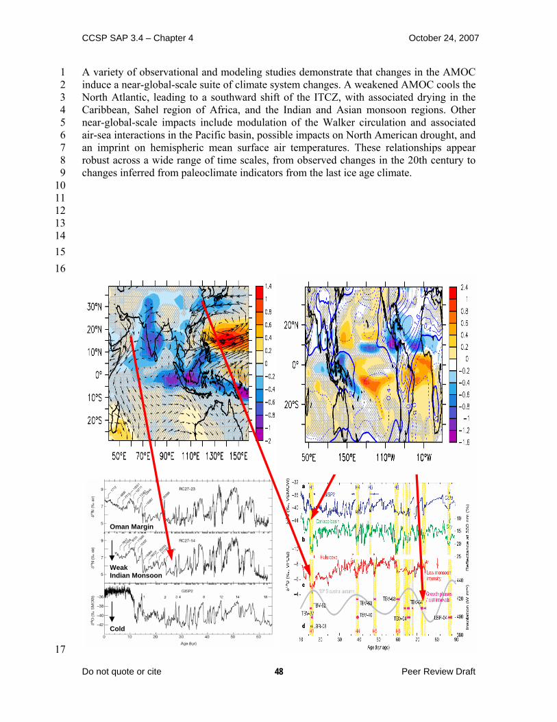
CCSP SAP 3.4 – Chapter 4 October 24, 2007
1 2 3 4 5 6 7 8 9
10 11 12 13 14 15 16
17
A variety of observational and modeling studies demonstrate that changes in the AMOC induce a near-global-scale suite of climate system changes. A weakened AMOC cools the North Atlantic, leading to a southward shift of the ITCZ, with associated drying in the Caribbean, Sahel region of Africa, and the Indian and Asian monsoon regions. Other near-global-scale impacts include modulation of the Walker circulation and associated air-sea interactions in the Pacific basin, possible impacts on North American drought, and an imprint on hemispheric mean surface air temperatures. These relationships appear robust across a wide range of time scales, from observed changes in the 20th century to changes inferred from paleoclimate indicators from the last ice age climate.
Oman Margin
Cold
Weak Indian Monsoon
Do not quote or cite Peer Review Draft
48

CCSP SAP 3.4 – Chapter 4 October 24, 2007
Figure 4.14. Comparison of simulated changes in response to the weakening of the AMOC using the Geophysical Fluid Dynamics Laboratory (GFDL) coupled model (CM2.0) with paleorecords. Upper left (Zhang and Delworth, 2005): Simulated summer precipitation change (color shading) and surface wind change (black vectors) over the Indian and eastern China regions. Upper right (Zhang and Delworth, 2005): Simulated annual mean precipitation change and sea-level pressure change (contour). Negative values correspond to a reduction of precipitation. Lower left (Altabet et al., 2002): The δ15N records for denitrification from sediment cores from the Oman margin in the Arabian Sea were synchronous with D-O oscillations recorded in Greenland ice cores (GISP2) during the last glacial period, i.e., the reduced denitrification, indicating weakened Indian summer monsoon upwelling, occurred during cold Greenland stadials. Lower right (Wang et al., 2004): Comparison of the growth patterns of speleothems from the northeastern Brazil (d) with (a) δ18O values of Greenland ice cores (GISP2), (b) Reflectance of the Cariaco basin sediments from ODP Hole 1002C (Peterson et al., 2000), (c) δ18O values of Hulu cave stalagmites (Wang et al., 2001). The modeled global
1 2 3 4 5 6 7 8 9
10 11 12 13 14 15
Do not quote or cite Peer Review Draft
49

CCSP SAP 3.4 – Chapter 4 October 24, 2007
1 2 3 4 5 6 7 8 9
10 11 12 13
14 15
response to the weakening of the AMOC (Zhang and Delworth, 2005) is consistent with all these synchronous abrupt climate changes found from Oman margin, Hulu Cave, Cariaco basin, and northeastern Brazil during cold Greenland stadials, i.e., drying at the Cariaco Basin, weakening of the Indian and Asian summer monsoon, and wetting in northeastern Brazil (red arrows). Abbreviations: %, percent; ‰, per mil; SMOW, Standard Mean Ocean Water; kyr, thousand years ago; H1, H4, H5, H6, Heinrich events; W m-2, watts per square meter; nm, nanometer. Figure 4.15. Left: various observed (OBS) quantities with an apparent association with the AMO. Right: Simulated responses of various quantities to AMO-like fluctuations in the Atlantic Ocean from a hybrid coupled model (adapted from Zhang and Delworth, 2006). Dashed green lines are unfiltered values, while the read and blue color-shaded values denote low-pass filtered values. Blue shaded regions indicate values below their
long-term mean, while red shading denotes values above their long-term mean. The vertical blue lines denotes transitions between warm and cold phases of the AMO. Time
Do not quote or cite Peer Review Draft
50

CCSP SAP 3.4 – Chapter 4 October 24, 2007
Do not quote or cite Peer Review Draft
51
1 2 3 4 5 6 7 8 9
10
in calendar years is along the bottom axis. (a), (e) AMO Index, a measure of SST over the North Atlantic. Positive values denote an unusually warm North Atlantic. (b), (f) Normalized summer rainfall anomalies over the Sahel (20oW.-40oE.,10-20oN.). (c), (g) Normalized summer rainfall over west-central India (65-80oE.,15-25oN.). (d) Number of major Atlantic Hurricanes from the HURDAT data set. The brown lines denote the vertical shear of the zonal (westerly) wind (multiplied by -1) derived from the ERA-40 reanalysis, i.e., the difference in the zonal wind between 850 and 200 hectopascals (hPa) over the south-central part of the main development region (MDR) for tropical storms (10-14oN.,70-20oW.). (h) Vertical shear of the simulated zonal wind (multiplied by -1), calculated as in (d).
11 12 13 14 15 16 17 18 19
Figure 4.16. These panels (adapted from Sutton and Hodson, 2005) show the simulated response of various fields to an idealized AMO SST anomaly using the HADAM3 atmosphere general circulation model. Results are time-means for the August-October period. (a) Sea level pressure, units are pascals (Pa), with an interval of 15 Pa. (b) Precipitation, units are millimeters per day. (c) Surface air temperature, units are kelvin. .

CCSP SAP 3.4 – Chapter 4 October 24, 2007
7 WHAT FACTORS THAT INFLUENCE THE OVERTURNING CIRCULATION ARE LIKELY TO CHANGE IN THE FUTURE, AND WHAT IS THE PROBABILITY THAT THE OVERTURNING CIRCULATION WILL CHANGE?
1 2 3 4 5 6 7 8 9
10 11 12 13 14 15 16 17 18 19 20 21 22 23 24 25
As noted in the Intergovernmental Panel for Climate Change (IPCC) 4th assessment report (AR4), all climate model projections under increasing greenhouse gases lead to an increase in high-latitude temperature as well as an increase in high-latitude precipitation (Meehl et al., 2007). Both warming and freshening tend to make the high-latitude surface waters less dense, thereby increasing their stability and inhibiting convection. In the IPCC AR4, 19 coupled atmosphere-ocean models contributed projections of future climate change under the SRES A1B scenario (Meehl et al., 2007). Of these, 16 models did not use flux adjustments (all except CGCM3.1, INM-CM3.0, and MRI-CGCM2.3.2). In making their assessment, Meehl et al. (2007) noted that several of the models simulated a late 20th century MOC strength that was inconsistent with present-day estimates: 14-18 Sv at 24°N. (Ganachaud and Wunsch, 2000; Lumpkin and Speer, 2003); 13-19 Sv at 48° N. (Ganachaud, 2003); maximum values of 17.2 Sv (Smethie and Fine, 2001) and 18 Sv (Talley et al., 2003) with an error of ± 3-5 Sv. They did not use the MOC from these models in making their assessment. The full range of late 20th century estimates of the Atlantic MOC strength (12-23 Sv), is spanned by the model simulations (Fig.4.17; Schmittner et al., 2005; Meehl et al., 2007). The models further project a decrease in the MOC strength of between 0% and 50%, with a multimodel average of 25%, over the course of the 21st century. None of the models simulated an abrupt shutdown of the MOC during the 21st century.
26 27 28 29 30 31 32
Figure 4.17. The Atlantic meridional overturning circulation (MOC) at 30°N. from the 19 coupled atmosphere-ocean models assessed in the IPCC AR4. The SRES A1B emissions scenario was used from 1999 to 2100. Those model projections that continued to 2200 retained the year 2100 radiative forcing for the remainder of the integration. Observationally based estimates of the late 20th century MOC strength are also shown on the left as black bars. Taken from Meehl et al. (2007) as originally adapted from
Do not quote or cite Peer Review Draft
52

CCSP SAP 3.4 – Chapter 4 October 24, 2007
Schmittner et al. (2005). 1 2 3 4 5 6 7 8 9
10 11 12 13 14 15 16 17 18 19 20 21 22 23 24 25 26 27 28 29 30 31 32 33 34 35 36 37 38 39 40 41 42 43 44 45 46
Schneider et al. (2007) extended the analysis of Meehl et al. (2007) by developing a multimodel average in which the individual model simulations were weighted a number of ways. The various weighting estimates were based on an individual model’s simulation of the contemporary ocean climate, and in particular its simulated fields of temperature, salinity, pycnocline depth, as well as its simulated Atlantic MOC strength. Their resulting best estimate 21st century MOC weakening of 25-30% was invariant to the weighting scheme used and is consistent with the simple multimodel mean of 25% obtained in the IPCC AR4. In early versions of some coupled atmosphere-ocean models, (e.g., Dixon et al., 1999), increased high-latitude precipitation dominated over increased high-latitude warming in causing the projected weakening of the MOC under increasing greenhouse gases, while in others (e.g., Mikolajewicz and Voss, 2000), the opposite was found. However, Gregory et al. (2005) undertook a recent model intercomparison project in which, in all 11 models analyzed, the MOC reduction was caused more by changes in surface heat flux than changes in surface fresh-water flux. Weaver et al. (2007) extended this analysis by showing that in one model, this conclusion was independent of the initial mean climate state. A number of stabilization scenarios have been examined using both coupled atmosphere-ocean general circulation models (AOGCMs) (Stouffer and Manabe, 1999; Voss and Mikolajewicz, 2001; Stouffer and Manabe, 2003; Wood et al., 2003; Yoshida et al., 2005; Bryan et al., 2006) as well as earth system models of intermediate complexity (EMICs) (Meehl et al., 2007). Typically the atmospheric CO2 concentration in these models is increased at a rate of 1%/year to either two times or four times the preindustrial level of atmospheric CO2, and held fixed thereafter. In virtually every simulation, the MOC reduces but recovers to its initial strength when the radiative forcing is stabilized at two times or four times the preindustrial levels of CO2. Only one early flux-adjusted model simulated a complete shutdown, and even this was not permanent (Manabe and Stouffer, 1994; Stouffer and Manabe, 2003). The only model to exhibit a permanent cessation of the MOC in response to increasing greenhouse gases was an intermediate complexity model which incorporates a zonally averaged ocean component (Meehl et al., 2007). Historically, coupled models that eventually lead to a collapse of the MOC under global warming conditions have fallen into two categories: (1) flux-adjusted coupled general circulation models and (2) intermediate-complexity models with zonally averaged ocean components. Both suites of models are known to be more sensitive to fresh-water perturbations. In the first class of models, a small perturbation away from the present climate leads to large systematic errors in the salinity fields (as large flux adjustments are applied) that can build up to cause abrupt MOC transitions. In the second class of models, the convection and sinking of water masses are coupled (there is no horizontal structure). The newer models assessed in the IPCC AR4 typically do not involve flux adjustments and have more stable projections of the future evolution of the MOC.
Do not quote or cite Peer Review Draft
53

CCSP SAP 3.4 – Chapter 4 October 24, 2007
1 2 3 4 5 6 7 8 9
10 11 12 13 14 15 16 17 18 19 20 21 22 23 24 25 26 27 28 29 30 31 32 33 34 35 36 37 38 39 40 41 42 43 44 45
One of the most misunderstood issues concerning the future of the AMO under anthropogenic climate change is its often cited potential to cause the onset of the next ice age. A relatively solid understanding of glacial inception exists wherein a change in seasonal incoming solar radiation (warmer winters and colder summers), which is associated with changes in the Earth’s axial tilt, longitude of perihelion, and the precession of its elliptical orbit around the sun, is required. This small change must then be amplified by albedo feedbacks associated with enhanced snow and ice cover, vegetation feedbacks associated with the expansion of tundra, and greenhouse gas feedbacks associated with the uptake (not release) of carbon dioxide and reduced release or increased destruction rate of methane. As discussed by Berger and Loutre (2002) and Weaver and Hillaire Marcel (2004a,b), it is not possible for global warming to cause an ice age. Wood et al. (1999), using HadCM3 with sufficient resolution to resolve Denmark Strait overflow, performed two transient simulations starting with a preindustrial level of atmospheric CO2 and subsequently increasing it at a rate of 1% or 2% per year. Convection and overturning in the Labrador Sea ceased in both these experiments while deep-water formation persisted in the Nordic seas. As the climate warmed, the Denmark Strait overflow water became warmer and hence lighter, so that the density contrast between it and the deep Labrador Sea water (LSW) was reduced. This made the deep circulation of the Labrador Sea collapse, while Denmark Straight overflow remained unchanged, a behavior suggested from the paleoreconstructions of Hillaire-Marcel et al. (2001) for the Last Interglacial (Eemian). The results of Hillaire-Marcel et al. (2001) suggest that the modern situation, with active LSW formation, has apparently no analog throughout the last glacial cycle, and thus appears a feature exclusive to the present interglacial. Results similar to those of Wood et al. (1999) were found by Hu et al. (2004), although Hu et al. (2004) also noted a significant increase in Greenland–Iceland–Norwegian (GIN) Sea convection as a result of enhanced inflow of saline North Atlantic water, and reduced outflow of sea ice from the Arctic. Some coupled models, on the other hand, found significant reductions in convection in the GIN Sea in response to increasing atmospheric greenhouse gases (Bryan et al., 2006; Stouffer et al., 2006). A cessation of LSW formation by 2030 was also found in high-resolution ocean model simulations of the Atlantic Ocean driven by surface fluxes from two coupled atmosphere-ocean climate models (Schweckendiek and Willebrand, 2005). Cottet-Puinel et al. (2004) obtained similar results to Wood et al. (1999) concerning the transient cessation of LSW formation and further showed that LSW formation eventually reestablished upon stabilization of anthropogenic greenhouse gas levels. The same model experiments of Wood et al. (1999) suggest that the freshening North Atlantic surface waters presently observed (Curry et al., 2003) is associated with a transient increase of the AMO (Wu et al., 2004). Such an increase would be consistent with findings of Latif et al. (2006), who argued that their analysis of ocean observations and model simulations supported the notion of a slight MOC strengthening since the 1980s.
Do not quote or cite Peer Review Draft
54

CCSP SAP 3.4 – Chapter 4 October 24, 2007
Do not quote or cite Peer Review Draft
55
The best estimate of sea level rise from 1993 to 2003 associated with mass loss from the Greenland ice sheet is 0.21 ± 0.07 mm yr–1
(Bindoff et al., 2007). This converts to only 0.0015 to 0.0029 Sv of fresh-water forcing, an amount that is too small to affect the MOC in models (see Weaver and Hillaire-Marcel, 2004a; Jungclaus et al., 2006). Recently, Velicogna and Wahr (2006) analyzed the Gravity Recovery and Climate Experiment (GRACE) satellite data to infer an acceleration of Greenland ice loss from April 2002 to April 2006 corresponding to 0.5 ± 0.1 mm/yr of global sea level rise. The equivalent 0.004–0.006 Sv of fresh-water forcing is once more too small to affect the MOC in models. Stouffer et al. (2006) undertook an intercomparison of 14 coupled models subject to a 0.1-Sv fresh-water perturbation (17 times the upper estimate from GRACE data) applied for 100 years to the northern North Atlantic Ocean. In all cases, the models exhibited a weakening of the MOC (by a multimodel mean of 30% after 100 years), and none of the models simulated a shutdown. Ridley et al. (2005) elevated greenhouse gas levels to four times preindustrial values and retained them fixed thereafter to investigate the evolution of the Greenland Ice sheet in their coupled model. They found a peak melting rate of about 0.1 Sv, which occurred early in the simulation, and noted that this perturbation had little effect on the MOC. Jungclaus et al. (2006) independently applied 0.09 fresh-water forcing along the boundary of Greenland as an upper-bound estimate of potential external fresh-water forcing from the melting of the Greenland ice sheet. Under the SRES A1B scenario they, too, only found a weakening of the MOC with a subsequent recovery in its strength. They concluded that Greenland ice sheet melting would not cause abrupt climate change in the 21st century.
1 2 3 4 5 6 7 8 9
10 11 12 13 14 15 16 17 18 19 20 21 22 23 24 25 26 27 28 29 30 31 32 33 34 35 36 37 38 39 40 41 42 43
Based on our analysis, we conclude that it is very likely that the strength of the MOC will decrease over the course of the 21st century. Both weighted and unweighted multimodel ensemble averages under an SRES A1B future emission scenario suggest a best estimate of 25-30% reduction in the overall MOC strength. Associated with this reduction is the possible cessation of LSW water formation. In models where the MOC weakens, warming still occurs downstream over Europe due to the radiative forcing associated with increasing greenhouse gases (Gregory et al., 2005; Stouffer et al., 2006). No model under idealized (1%/year or 2%/year increase) or SRES scenario forcing exhibits an abrupt collapse of the MOC during the 21st century, even accounting for estimates of accelerated Greenland ice sheet melting. We conclude that it is very unlikely that the MOC will undergo an abrupt transition during the course of the 21st century. Based on available model simulations and sensitivity analyses, estimates of maximum Greenland ice sheet melting rates, and our understanding of mechanisms of abrupt climate change from the paleoclimate record, we further conclude it is unlikely that the MOC will collapse beyond the end of the 21st century as a consequence of global warming, although the possibility cannot be entirely excluded.

CCSP SAP 3.4 – Chapter 4 October 24, 2007
8 WHAT ARE THE OBSERVATIONAL AND MODELING REQUIREMENTS NECESSARY TO UNDERSTAND THE OVERTURNING CIRCULATION AND EVALUATE FUTURE CHANGE?
1 2 3 4 5 6 7 8 9
10 11 12 13 14 15 16 17 18 19 20 21 22 23 24 25 26 27 28 29 30 31 32 33 34 35 36 37 38 39 40 41 42 43 44 45 46
It has been shown in this chapter that the AMOC plays a vital role in the climate system. In order to more confidently predict future changes – especially the possibility of abrupt change – we need to better understand the AMOC and the mechanisms governing its variability and sensitivity to forcing changes. Improved understanding of the AMOC comes at the interface between observational and theoretical studies. In that context, theories can be tested, oftentimes using numerical models, against the best available observational data. The observational data can come from the modern era or from proxy indicators of past climates. We describe in this section a suite of activities that are necessary to increase our understanding of the AMOC and to more confidently predict its future behavior. While the activities are noted in separate categories, the true advances in understanding – leading to a predictive capability – come in the synthesis of the various activities described below, particularly in the synthesis of modeling and observational analyses. 8.1 Sustained Modern Observing System We currently lack a long-term, sustained observing system for the AMOC. Without this in place, our ability to detect and predict future changes of the AMOC – and their impacts – is very limited. The RAPID project may be viewed as a prototype for such an observing system. The following set of activities is therefore needed:
• Research to delineate what would constitute an efficient, robust observational network for the AMOC. This could include studies in which model results are sampled according to differing observational networks, thereby evaluating the utility of those networks for observing the AMOC and guiding the development of new observational networks and the enhancement of existing observational networks.
• Sustained deployment over decades of the observational network identified above to robustly measure the AMOC
• Focused observational programs as part of process studies to improve understanding of physical processes of importance to the AMOC, such as ocean-atmosphere coupling, mixing processes, and deep overflows. These should lead to improved representation of such processes in numerical models.
8.2 Acquisition and Interpretation of Paleoclimate Data While the above stresses current observations, much can be learned from the study of ancient climates that provide insights into the past behavior of the AMOC. We need to develop paleoclimate data sets that allow robust, quantitative reconstructions of past ocean circulations and their climatic impacts. Therefore, the following set of activities is needed:
Do not quote or cite Peer Review Draft
56

CCSP SAP 3.4 – Chapter 4 October 24, 2007
• Acquisition and analysis of high-resolution records from the Holocene that can 1 provide insight on decadal to centennial time scales of AMOC-related climate variability. This is an important baseline against which to judge future change.
2 3
5 6 7 8 9
10 11 12 13 14 15 16 17 18 19 20 21 22 23 24 25 26 27 28 29 30 31 32 33 34 35 36 37 38 39 40 41 42 43 44 45 46
• Acquisition and analysis of paleoclimate records to document past changes in the 4 AMOC, including both glacial and nonglacial conditions. These will provide a more robust measure of the response of the AMOC to changing radiative forcing and will allow new tests of models. Our confidence in predictions of future AMOC changes is enhanced to the extent that models faithfully simulate such past AMOC changes.
• More detailed assessment of the past relationship between AMOC and climate, especially the role of AMOC changes in abrupt climate change.
• Acquisition and analysis of paleoclimate records that can provide improved estimates of past changes in meltwater forcing. This information can lead to improved understanding of the AMOC response to fresh-water input and can help to better constrain models.
8.3 Improvement and Use of Models Models provide our best tools for predicting future changes in the AMOC and are an important pathway toward increasing our understanding of the AMOC, its variability, and its sensitivity to change. Such insights are limited, however, by the fidelity of the models employed. There is an urgent need both to (1) improve the models we use and (2) use models in innovative ways to increase our understanding of the AMOC. Therefore, the following set of activities is needed:
• Development of models with increased resolution in order to more faithfully represent the small-scale processes that are important for the AMOC. The models used for the IPCC AR4 assessment had oceanic resolution of order 50-100 km in the horizontal, with 30-50 levels in the vertical. In reality, processes with spatial scales of several kilometers (or less) are important for the AMOC.
• Development of models with improved numerics and physics, especially those that appear to influence the AMOC. In particular, there is a need for improved representation of small-scale processes that significantly impact the AMOC. For example, overflows of dense water over sills in the North Atlantic are an important feature for the AMOC, and their representation in models needs to be improved.
• Design and execution of innovative numerical experiments in order to (1) shed light on the mechanisms governing variability and change of the AMOC,(2) estimate the inherent predictability of the AMOC, and(3) develop methods to realize that predictability. The use of multimodel ensembles is particularly important.
• Development and use of improved data assimilation systems for providing estimates of the current and past states of the AMOC, as well as initial conditions for prediction of the future evolution of the AMOC.
• Development of prototype prediction systems for the AMOC. These prediction systems will start from the observed state of the AMOC and use the best possible
Do not quote or cite Peer Review Draft
57

CCSP SAP 3.4 – Chapter 4 October 24, 2007
1 2 3 4 5 6 7 8 9
10 11 12 13 14 15 16 17 18 19 20 21 22 23 24 25 26 27 28 29 30 31 32 33 34
models, together with projections of future changes in atmospheric greenhouse gases and aerosols, to make the best possible projections for the future behavior of the AMOC. Such a prediction system would serve as a warning system for an abrupt change in the AMOC.
8.4 Projections of Future Changes in Radiative Forcing and Related Impacts One of the motivating factors for the study of AMOC behavior is the possibility of abrupt change in the future driven by increasing greenhouse gas concentrations. In order to evaluate the likelihood of such an abrupt change, it is crucial to have available the best possible projections for future changes in radiative forcing, especially those changes in radiative forcing due to human activity. This includes not only greenhouse gases, which tend to be well mixed and long lived in the atmosphere, but also aerosols, which tend to be shorter lived with more localized spatial patterns. The short residence time of aerosols implies that their atmospheric concentration is closely linked on short time scales to the emissions. This raises the possibility, in contrast to greenhouse gases, of large changes in aerosol concentrations on short time scales. Thus, rapid changes in aerosol concentration could be a driver for abrupt changes, and realistic projections of aerosol concentrations and their climatic effects are important for AMOC projections. One of the important controls on the AMOC is the fresh-water flux into the Atlantic. One important component is the inflow of fresh water from rivers surrounding the Arctic. For example, observations (Peterson et al., 2002) have shown an increase during the 20th century of Eurasian river discharge into the Arctic. For the prediction of AMOC changes it is crucial to have complete observations of changes in the high-latitude hydrologic cycle, including precipitation, evaporation, and river discharge, as well as water released into the Atlantic from the Greenland ice sheet and from glaciers. This topic is discussed more extensively in Chapter 2.
Do not quote or cite Peer Review Draft
58

CCSP SAP 3.4 – Chapter 4 October 24, 2007
BOX 1: How do we measure the MOC? 1 2 3 4 5 6 7 8 9
10
11 12 13 14 15 16 17
18 19 20 21 22 23 24 25 26 27 28 29 30
31 32 33 34 35 36 37 38 39 40 41 42 43 44 45
Observational estimates of the MOC require the measurement, or inference, of all components of the meridional circulation across a basinwide section. In principle, if direct measurements of the meridional velocity profile are available at all locations across the section, the calculation of the MOC is straightforward: the velocity is zonally integrated across the section at each depth, and the resulting vertical transport profile is then summed over the northward-moving part of the profile (which is typically the upper ~1,000 m for the Atlantic) to obtain the strength of the MOC.
In practice, available methods for measuring the absolute velocity across the full width of a transbasin section are either prohibitively expensive or of insufficient accuracy to allow a reliable estimate of the MOC. Thus, the meridional circulation is typically broken down into several discrete components that can either be measured directly (by current observations), indirectly (by geostrophic calculations based on hydrographic data), or inferred from wind observations (Ekman transports) or mass-balance constraints.
An illustration of this breakdown is shown in the Box 1 figure for the specific situation of the subtropical Atlantic Ocean near 26ºN., where the RAPID-MOC array is deployed and where a number of basinwide hydrographic sections have been occupied. The measured transport components include (1) direct measurement of the flow though the Straits of Florida and (2) geostrophic mid-ocean flow derived from density profiles at the eastern and western sides of the ocean, relative to an unknown constant or "reference velocity." A third component is the ageostrophic flow in the surface layer driven by winds (the Ekman transport), which can be estimated from available wind-stress products. The only remaining unmeasured component is the depth-independent (or "barotropic") mid-ocean flow, which is inferred by requiring an overall mass balance across the section. Once combined, these components define the basinwide transport profile and the MOC strength.
The above breakdown is effective because it takes advantage of the spatially integrating nature of geostrophic computations across the interior of the ocean and limits the need for direct velocity or transport measurements to narrow regions near the coastal boundaries where swift currents may occur (in particular, in the western boundary region). The application is similar for individual hydrographic sections or moored density arrays such as used in RAPID, except that the moored arrays can provide continuous estimates of the interior flow instead of single snapshots in time. Each location where the MOC is to be measured requires a sampling strategy tuned to the section's topography and known circulation features, but the methodology is essentially the same (Hall and Bryden, 1982; Bryden et al., 1991; Cunningham et al., 2007). Inverse models (see Section 2.1) follow a similar approach but use a formalized set of constraints with specified error tolerances (e.g., overall mass balance, western boundary current transports, property fluxes) to optimally determine the reference velocity distribution across a section (Wunsch, 1996).
Do not quote or cite Peer Review Draft
59

CCSP SAP 3.4 – Chapter 4 October 24, 2007
1 2 3 4
5 6 7 8 9
10 11 12 13 14 15 16 17 18 19
Box 1 Figure: Circulation components required to estimate the MOC. The figure depicts the approximate topography along 24-26ºN. and the strategy employed by the RAPID monitoring array. The transport of the western boundary current is continuously monitored by a calibrated submarine cable across the Straits of Florida. Hydrographic moorings (depicted by white vertical lines) near the east and west sides of the basin monitor the (relative) geostrophic flow across the basin as well as local flow contributions adjacent to the boundaries. Ekman transport is estimated from satellite wind observations. A uniform velocity correction is included in the interior ocean to conserve mass across the section. (Figure courtesy of J. Hirschi, NOC, Southampton, U.K.)
Do not quote or cite Peer Review Draft
60

CCSP SAP 3.4 – Chapter 4 October 24, 2007
Do not quote or cite Peer Review Draft
61
BOX 2: Would a collapse of the AMOC lead to cooling of Europe and North America?
1 2 3 4 5 6 7 8 9
10 11 12 13 14 15 16 17 18 19 20
One of the motivations behind the study of abrupt change in the AMOC is its potential influence on the climates of North America and Western Europe. Some reports, particularly in the media, have suggested that a shutdown of the AMOC in response to global warming could plunge Western Europe and even North America into conditions much colder than our current climate. Based on our current understanding of the climate system, such a scenario appears very unlikely. On the multidecadal to century time scale, it is very likely that Europe and North America will warm in response to increasing greenhouse gases (although natural variability and regional shifts could lead to periods of decadal-scale cooling in some regions). A significant weakening of the AMOC in response to global warming would moderate that long-term warming trend. If a complete shutdown of the AMOC were to occur (viewed as very unlikely, as described in this assessment), the reduced ocean heat transport could lead to a net cooling of the ocean by several degrees in parts of the North Atlantic, and possibly 1 to 2 degrees C over portions of extreme western and northwestern Europe. However, even in such an extreme (and very unlikely) scenario, a multidecadal to century-scale warming trend in response to increasing greenhouse gases would still be anticipated over most of North America, eastern and southern Europe, and Asia.

CCSP SAP 3.4 – Chapter 4 October 24, 2007
BOX 3: Possibility for abrupt transitions in sea ice cover 1
2
3 4 5 6 7 8 9
10 11 12
13 14 15 16 17 18
19 20 21 22 23 24 25 26 27
28 29 30 31 32 33 34 35 36 37 38
Because of certain properties of sea ice, it is quite natural to expect that the ice cover might undergo rapid change in response to modest forcing. Sea ice has a strong inherent threshold in that its existence depends on the freezing temperature of sea water. Additionally, strong positive feedbacks associated with sea ice act to accelerate its change. The most notable of these is the surface albedo feedback resulting from changes in total cover and surface properties of the ice that modify the surface reflection of solar radiation. For example, reductions in ice cover expose the dark underlying ocean, reducing the reflectivity of the surface. This allows more solar radiation to be absorbed, enhancing the warming and leading to further ice melt.
Simple models have indeed shown abrupt, nonlinear behavior in the sea ice cover. For example, box model studies have shown a “switch-like” behavior in the ice cover (Gildor and Tziperman, 2001). Since the ice cover modifies ocean-atmosphere moisture exchange, this in turn affects the source of water for ice sheet growth within these models with possible implications for glacial cycles.
Other simple models, specifically diffusive climate models, also exhibit rapid sea ice change. These models simulate that an ice cap of sufficiently small size is unstable. This “small ice cap instability” (SICI) (North, 1984) leads to an abrupt transition to ice-free conditions under a gradually warming climate. Recently, Winton (2006) examined coupled climate model output and found that of two models that simulate a complete loss of Arctic ice cover in response to increased CO2 forcing, one had SICI-like behavior in which a nonlinear response of surface albedo to the warming climate resulted in an abrupt loss of Arctic ice. The other model showed a more linear response.
Perhaps more important for near-term (50-100 year) climate change is the possibility for a rapid transition to seasonally ice-free Arctic conditions. Holland et al. (2006) showed that rapid September Arctic ice loss, typically 4 times larger than comparable observed trends, was exhibited by about 50% of a group of coupled models that participated in the Intergovernmental Panel on Climate Change Fourth Assessment Report for some standard future forcing scenario. In one case, a transition from conditions similar to today to a near-ice-free September extent occurred in a decade. This abrupt ice loss resulted from the interaction of large intrinsic variability and anthropogenically forced change, which allows periods of relative stability (when the natural variations counteract the forced change) followed by instances of abrupt retreat (when the two work in concert).
Do not quote or cite Peer Review Draft
62

CCSP SAP 3.4 – Chapter 4 October 24, 2007
1
2 3 4 5 6 7 8 9
10 11 12 13 14 15 16 17 18 19 20 21 22 23 24 25 26 27 28 29 30 31 32 33 34 35 36 37 38 39 40 41 42 43 44 45 46 47 48 49 50 51 52 53
REFERENCES
Adcroft, A., J.R. Scott, and J. Marotzke. 2001. Impact of geothermal heating on the global ocean circulation. J. Geophys. Res. 28 (9), 1735-1738.
Adkins, J.F., K. McIntyre, and D.P.Schrag. 2002. The salinity, temperature and δ18O of the glacial deep ocean. Science 298: 1769-1773.
Ahn, J., and E.J. Brook. 2007. Atmospheric CO2 and climate from 65 to 30 ka B.P., Geophys. Res. Let., 34, L10703, doi:10.1029/2007GL029551.
Alley, R.B., and P.U. Clark. 1999. The deglaciation of the northern hemisphere: A global perspective, Ann. Rev. Earth Planet. Sci., 27, 149-182.
Altabet, M.A., M.J. Higginson, and D.W. Murray. 2002. The effect of millennial-scale changes in Arabian Sea denitrification on atmospheric CO2. Nature, 415, 159-162.
Arz, H., J. Patzold, and G. Wefer. 1998. Correlated millennial-scale changes in surface hydrography and terrigenous sediment yield inferred from last-glacial marine deposits off northeastern Brazil, Quat. Res., 50, 157-166.
Barnett, T.P., L. Dumenil, U. Schlese, E. Roeckner, and M. Latif.1989. The effect of Eurasian snow cover on regional and global climate variations, J. Atmos. Sci., 46, 661-685.
Bartoli, G., M. Sarnthein, and M. Weinelt.2006. Late Pliocene millennial-scale climate variability in the northern North Atlantic prior to and after the onset of Northern Hemisphere glaciation, Paleoceanography, 21, PA4205, doi:10.1029/2005PA001185.
Behl, R. and J.P. Kennett. 1996. Brief interstadial events in the Santa Barbara basin, NE Pacific, during the past 60 kyr. Nature, 379, 243-246.
Bender, M, T. Sowers, M.-L. Dickson, J. Orchardo, P. Grootes, P.A. Mayewski, and D.A. Meese. 1994. Climate correlations between Greenland and Antarctica during the past 100,000 years, Nature, 372, 663-666.
Bender, M.L., B. Malaize, J. Orchardo, T. Sowers, and J. Jouzel. 1999. High-precision correlations of Greenland and Antarctic ice core records over the last 100 kyr, in Mechanisms of Global Climate Change at Millennial Time Scales, Geophys. Monogr. Ser., vol. 112, edited by P.U. Clark, R.S. Webb, and L.D. Keigwin, p. 149-164, AGU, Washington, D.C.
Benway, H.M., A.C. Mix, B.A. Haley, and G.P. Klinkhammer. 2006. Eastern Pacific Warm Pool paleosalinity and climate variability: 0-30 kyr, Paleoceanography, 21, PA3008, doi:10.1029/2005PA001208.
Berger, A. and M.F. Loutre, 2002: An exceptionally long Interglacial ahead? Science, 297, 1287-1288. Bickert, T., and A. Mackensen. 2004. Late Glacial to Holocene changes in South Atlantic deep water
circulation, in The South Atlantic in the Late Quaternary: Reconstruction of Material Budget and Current Systems, edited by G. Wefer, et al., p. 671-693, Springer-Verlag, Berlin.
Bindoff, N.L., J. Willebrand, V. Artale, A, Cazenave, J. Gregory, S. Gulev, K. Hanawa, C. Le Quéré, S. Levitus, Y. Nojiri, C.K. Shum, L.D. Talley and A. Unnikrishnan, 2007: Observations: Oceanic climate change and sea level, in Climate change 2007: The physical science basis. Contribution of Working Group I to the Fourth Assessment Report of the Intergovernmental Panel on Climate Change [Solomon, S., D. Qin, M. Manning, Z. Chen, M. Marquis, K.B. Averyt, M. Tignor and H.L. Miller (eds.)]. Cambridge University Press, Cambridge, United Kingdom and New York, NY, USA, 996 p.
Black D.E., L.C. Peterson, J.T. Overpeck, A. Kaplan, M.N. Evans, M. Kashgarian. 1999, Eight centuries of North Atlantic Ocean atmosphere variability, Science, 286, 1709-1713.
Blunier, T., and E.J. Brook. 2001. Timing of millennial-scale climate change in Antarctica and Greenland during the last glacial period, Science, 291, 109-112.
Blunier, T., and others. 1998. Asynchrony of Antarctic and Greenland climate change during the last glacial period, Nature, 394, 739-743.
Bond, G.C., and others. 1992. Evidence of massive discharges of icebergs into the North Atlantic Ocean during the last glacial period, Nature, 360, 245- 249.
Bond, G.C., W.S. Broecker, S. Johnsen, J. McManus, L. Labeyrie, J. Jouzel, and G. Bonani. 1993. Correlations between climate records from North Atlantic sediments and Greenland ice, Nature, 365, 143-147.
Do not quote or cite Peer Review Draft
63

CCSP SAP 3.4 – Chapter 4 October 24, 2007
1 2 3 4 5 6 7 8 9
10 11 12 13 14 15 16 17 18 19 20 21 22 23 24 25 26 27 28 29 30 31 32 33 34 35 36 37 38 39 40 41 42 43 44 45 46 47 48 49 50 51 52 53 54 55 56
Boning, C.W., M. Scheinert, J. Dengg, A. Biastoch, and A. Funk, 2006: Decadal variability of subpolar gyre transport and its reverberation in the North Atlantic overturning. Geophysical Research Letters, 33, 5.
Boyle, E.A. 1992. Cadmium and δ13C paleochemical ocean distributions during the stage 2 glacial maximum. Annual Review of Earth and Planetary Sciences 20: 245-287.
Boyle, E.A.. 2000. Is ocean thermohaline circulation linked to abrupt stadial/interstadial transitions? Quat. Sci. Rev., 19, 255-272.
Boyle E.A., and L.D., Keigwin.1982. Deep circulation of the North Atlantic over the last 200,000 years: geochemical evidence, Science, 218, 784-787.
Braconnot, P. and others. 2007. Results of PMIP2 coupled simulations of the Mid-Holocene and Last Glacial Maximum. Part I: Experiments and large-scale features. Climate of the Past 3, 261-277.
Broecker, W.S., G.C. Bond, M. Klas, E. Clark, and J. McManus. 1992. Origin of the northern Atlantic's Heinrich events, Clim. Dyn., 6, 265-273.
Bryan, F.O., G. Danabasoglua, N. Nakashikib, Y. Yoshidab, D.-H. Kimb, J. Tsutsuib, and S.C. Doney and others. 2006: Response of the North Atlantic thermohaline circulation and ventilation to increasing carbon dioxide in CCSM3. Journal of Climate, 19, 2382-2397.
Bryan, F.O., Hecht, M.W., and Smith, R.D. 2007. Resolution convergence and sensitivity studies with North Atlantic circulation models. Part I: The western boundary current system. Ocean Modelling 16: 141-159.
Bryden, H.L., D.H. Roemmich, and J.A. Church. 1991: Ocean heat transport across 24 degrees N in the Pacific. Deep-Sea Research Part A-Oceanographic Research Papers, 38, 297-324.
Bryden, H.L., H.R. Longworth, and S.A. Cunningham., 2005: Slowing of the Atlantic meridional overturning circulation at 25 degrees N. Nature, 438, 655-657.
Calov, R., A. Ganopolski, V. Petoukhov, and M. Claussen. 2002. Large-scale instabilities of the Laurentide ice sheet simulated in a fully coupled climate-system model, Geophys. Res. Lett., 29, 2216, doi:10.1029/2002GL016078.
Cane, M.A.. 1998. A role for the tropical Pacific, Science, 282, 59-61. Carton, J.A., G. Chepurin, X.H. Cao, and B. Giese, 2000: A Simple Ocean Data Assimilation analysis of
the global upper ocean 1950-95. Part I: Methodology. Journal of Physical Oceanography, 30, 294-309.
Charles, C.D., J. Lynch-Stieglitz, U.S. Ninneman, and R.G. Fairbanks. 1996. Climate connections between the hemispheres revealed by deep-sea sediment/ice core correlations, Earth Planet. Sci. Let., 142, 19-27.
Chiang, J.C.H., M. Biasutti, and D.S. Battisti. 2003. Sensitivity of the Atlantic Intertropical Convergence Zone to Last Glacial Maximum boundary conditions, Paleoceanography, 18, 1094, doi:10.1029/2003PA000916.
Clark, P.U., N.G. Pisias, T.S. Stocker, and A.J. Weaver. 2002. The role of the thermohaline circulation in abrupt climate change, Nature, 415, 863-869.
Clark, P.U., Hostetler, S.W., Pisias, N.G., Schmittner, A., and Meissner, K.J. 2007. Mechanisms for a ~7-kyr climate and sea-level oscillation during Marine Isotope Stage 3: American Geophysical Union Monograph, in press.
CLIMAP .1981. Seasonal reconstructions of the earth's surface at the Last Glacial Maximum, 18 p. Cottet-Puinel, M., A.J. Weaver, C. Hillaire-Marcel, A. de Vernal, P.U. Clark, and M. Eby. 2004: Variation
of Labrador Sea water formation over the last glacial cycle in a climate model of intermediate complexity. Quaternary Science Reviews, 23, 449-465.
Crowley, T.J. 1992. North Atlantic Deep Water cools the southern hemisphere, Paleoceanography, 7, 489-497.
Cuffey, K.M., and G.D. Clow. 1997. Temperature, accumulation, and ice sheet elevation in central Greenland through the last deglacial transition, Jour. Geophys. Res., 102, 26,383-26,396.
Cunningham, S.A., T. Kanzow, D. Rayner, M.O. Baringer, W.E. Johns, J. Marotzke, H. Longworth, E. Grant, J. Hirschi, L. Beal, C.S. Meinen, and H. Bryden. 2007: Temporal variability of the Atlantic meridional overturning circulation at 25°N, Science, in press.
Curry, R., B. Dickson, and I. Yashayaev. 2003. A change in the freshwater balance of the Atlantic Ocean over the past four decades, Nature, 426, 826-829
Curry W.B., and G.P. Lohmann. 1982. Carbon isotopic changes in benthic foraminifera from the western South Atlantic: Reconstructions of glacial abyssal circulation patterns, Quat. Res., 18, 218-235.
Do not quote or cite Peer Review Draft
64

CCSP SAP 3.4 – Chapter 4 October 24, 2007
1 2 3 4 5 6 7 8 9
10 11 12 13 14 15 16 17 18 19 20 21 22 23 24 25 26 27 28 29 30 31 32 33 34 35 36 37 38 39 40 41 42 43 44 45 46 47 48 49 50 51 52 53 54
Curry, W.B., and D.W. Oppo. 2005. Glacial water mass geometry and the distribution of δ13C of ΣCO2 in the western Atlantic Ocean, Paleoceanography, 20(1), PA1017.
Dahl, K.A., A.J. Broccoli, and R.J. Stouffer, 2005, Assessing the role of North Atlantic freshwater forcing in millennial scale climate variability: A tropical Atlantic perspective, Climate Dynamics, 24, 325-346.
Delworth, T.L., and M.E. Mann. 2000: Observed and simulated multidecadal variability in the Northern Hemisphere. Clim. Dyn., 16, 661-676.
Delworth, T.L., R. Zhang, and M.E. Mann. 2007. Decadal to centennial variability of the Atlantic from observations and models. AGU monograph Past and future changes of the ocean’s Meridional Overturning Circulation: Mechanisms and Impacts. Accepted.
Dengg, J., Beckmann, A., and Gerdes, R. 1996. The gulf stream separation problem, in Krauss, W., ed., The warmwatersphere of the North Atlantic Ocean. Gebruder-Borntrager, p. 253-290.
Denton, G.H., R.B. Alley, G.C. Comer, and W.S. Broecker. 2005. The role of seasonality in abrupt climate change, Quat. Sci. Rev., 24, 1159-1182.
Dickson, R.R., J. Lazier, J. Meincke, P. Rhines, and J. Swift. 1996. Long-term coordinated changes in the convective activity of the North Atlantic, Prog. Oceanogr., 38, 241-295
Dixon, K., T. Delworth, M. Spelman, and R. Stouffer. 1999. The influence of transient surface fluxes on North Atlantic overturning in a coupled GCM climate change experiment, Geophysical Research Letters, 26, 2749–2752.
Dokken, T. M., and E. Jansen. 1999. Rapid changes in the mechanism of ocean convection during the last glacial period, Nature, 401, 458-461.
Dong, B.W., R.T. Sutton, and A.A. Scaife. 2006. Multidecadal modulation of El Nino Southern Oscillation (ENSO) variance by Atlantic Ocean sea surface temperatures. Geophys. Res. Letters, 3, doi:10.1029/2006GL025766.
Dong B.W., and R.T. Sutton. 2007. Enhancement of ENSO variability by a weakened Atlantic thermohaline circulation in a coupled GCM, Journal of Climate ,in press.
Douville, H., and J.-F. Royer. 1996. Sensitivity of the Asian summer monsoon to an anomalous Eurasian snow cover with the Meteo-France GCM, Climate Dynamics, 12, 449-466.
Dowdeswell, J.A., M.A. Maslin, J.T. Andrews, and I.N. McCave. 1995. Iceberg production, debris rafting, and the extent and thickness of Heinrich layers (H-1, H-2) in North Atlantic sediments, Geology, 23, 301-304.
Duplessy J.-C., N.J. Shackleton, R.G. Fairbanks, L. Labeyrie, D. Oppo, and N. Kallel. 1988. Deepwater source variations during the last climatic cycle and their impact on the global deepwater circulation, Paleoceanography, 3, 343-360.
Elliot, M., L.D. Labeyrie, and J.-C. Duplessy. 2002. Changes in North Atlantic deep-water formation associated with the Dansgaard-Oeschger temperature oscillations (60-10 ka), Quat. Sci. Rev., 21, 1153-1165.
Enfield, D.B., A.M. Mestas-Nuñez, and P.J. Trimble. 2001: The Atlantic multidecadal oscillation and its relation to rainfall and river flows in the continental U.S., GRL, 28, 2077-2080.
EPICA Community Members. 2006. One-to-one coupling of glacial climate variability in Greenland and Antarctica, Nature, 444, 195-198.
Fluckiger, J., R. Knutti, and J.W.C. White. 2006. Oceanic processes as potential trigger and amplifying mechanisms for Heinrich events, Paleoceanography, 21, PA2014, doi:10.1029/2005PA001204,
Folland, C.K., T.N. Palmer, and D.E. Parker. 1986: Sahel rainfall and worldwide sea temperatures. Nature., 320, 602-607.
Ganachaud, A., 2003a: Large-scale mass transports, water mass formation, and diffusivities estimated from World Ocean Circulation Experiment (WOCE) hydrographic data. Journal of Geophysical Research-Oceans, 108, 24.
Ganachaud, A., 2003b: Error budget of inverse box models: The North Atlantic. Journal of Atmospheric and Oceanic Technology, 20, 1641-1655.
Ganachaud, A. and Wunsch, C. 2000. Improved estimates of global ocean circulation, heat transport, and mixing from hydrographic data. Nature, 408, 453-457.
Ganopolski, A., and S. Rahmstorf. 2001. Rapid changes of glacial climate simulated in a coupled climate model, Nature, 409, 153-158.
Do not quote or cite Peer Review Draft
65
CCSP SAP 3.4 – Chapter 4 October 24, 2007
1 2 3 4 5 6 7 8 9
10 11 12 13 14 15 16 17 18 19 20 21 22 23 24 25 26 27 28 29 30 31 32 33 34 35 36 37 38 39 40 41 42 43 44 45 46 47 48 49 50 51 52 53 54
Gherardi, J.M., and others. 2005. Evidence from the Northeastern Atlantic basin for variability in the rate of the meridional overturning circulation through the last deglaciation, Earth and Planetary Science Letters, 240, 3-4, 710-723.
Gildor, H., and E. Tziperman. 2001. A sea ice climate switch mechanism for the 100-kyr glacial cycles, J. Geophys. Res., 106, C5, 9117-9133.
Girton, J.G., and T.B. Sanford. 2003. Descent and modification of the overflow plume in the Denmark Strait, J. Phys. Oceanogr., 33, 7, 1351-1364
Gnanadesikan, A., R.D. Slater, P.S. Swathi, and G.K. Vallis. 2005. The energetics of ocean heat transport, J. Clim, 18, 2604-2616.
Goldenberg, S.B., C.W. Landsea, A M. Mestas-Nuñez, and W.M. Gray. 2001. The recent increase in Atlantic hurricane activity: Causes and implications, Science, 293, 474-479.
Gordon, A.L. 1986: Inter-ocean exchange of thermocline water. Journal of Geophysical Research-Oceans, 91, 5037-5046.
Gregory, J.M., and others. 2005. A model intercomparison of changes in the Atlantic thermohaline circulation in response to increasing atmospheric CO2 concentration, Geophys. Res. Lett., 32, L12703, doi: 10.1029/2005GL023209.
Grimm, E.C., W.A. Watts, G.L. Jacobson, Jr., B.C.S. Hansen, H. Almquist, A.C. Dieffenbacher-Krall. 2006. Evidence for warm wet Heinrich events in Florida, Quat. Sci. Rev., 25, 2197-2211.
Grootes, P.M., M. Stuiver, J.W.C. White, S.J. Johnsen, J. Jouzel. 1993. Comparison of oxygen isotope records from the GISP2 and GRIP Greenland ice cores, Nature, 366, 552-554.
Gupta, A.K., D.M. Anderson and J.T. Overpeck. 2003. Abrupt changes in the Asian southwest monsoon during the Holocene and their links to the North Atlantic Ocean, Nature, 421, 354-357.
Gwiazda, R.H., S.R. Hemming, and W.S. Broecker. 1996. Tracking the sources of icebergs with lead isotopes: The provenance of ocean-rafted debris in Heinrich Layer 2, Paleoceanography, 11, 77-93.
Hall, M.M., and H.L. Bryden. 1982. Direct estimates and mechanisms of ocean heat transport. Deep-Sea Research Part a-Oceanographic Research Papers, 29, 339-359.
Hallberg, R., and A. Gnanadesikan. 2006. The role of eddies in determining the structure and response of the wind-driven Southern Hemisphere overturning: Results from the Modeling Eddies in the Southern Ocean (MESO) Project, J. Phys. Oceanogr., 36, 2232-2252.
Haug, G.H., K.A. Hughen, D.M. Sigman, L.C. Peterson, and U. Röhl. 2001. Southward migration of the Intertropical Convergence Zone through the Holocene, Science 293, 1304-1308.
Heinrich, H. 1988. Origin and consequences of cyclic ice-rafting in the northeast Atlantic Ocean during the past 130,000 years, Quat. Res., 29, 142-152.
Hemming, S.R., W.S. Broecker, W.D. Sharp, G.C. Bond, R.H. Gwiazda, J.F. McManus, M. Klas, and I. Hajdas. 1998. Provenance of Heinrich layers in core V28–82, northeastern Atlantic: 40Ar-39Ar ages of ice-rafted hornblende, Pb isotopes in feldspar grains, and Nd-Sr-Pb isotopes in the fine sediment fraction, Earth Planet. Sci. Lett., 164, 317-333.
Hemming, S.R.. 2004. Heinrich events: Massive late Pleistocene detritus layers of the North Atlantic and their global climate imprint, Rev. Geophysics, 42, RG1005, doi:10.1029/2003RG000128.
Hendy, I.L., and J.P. Kennett. 2000. Dansgaard-Oeschger cycles and the California Current System: Planktonic foraminiferal response to rapid climate change in Santa Barbara Basin, Ocean Drilling Program hole 893A, Paleoceanography, 15, 30-42.
Hillaire-Marcel, C., and G. Bilodeau. 2000. Instabilities in the Labrador Sea water mass structure during the last climatic cycle, Can. Jour. Earth Sci., 37, 795-809.
Hillaire-Marcel, C., A. de Vernal, G. Bilodeau and A.J. Weaver. 2001. Absence of deep-water formation in the Labrador Sea during the last interglacial period. Nature, 410, 1073-1077.
Holland, M.M., C.M. Bitz, and B. Tremblay. 2006: Future abrupt reductions in the summer Arctic sea ice, Geophys. Res. Lett., 33, L23503, doi:10.1029/2006GL028024.
Hu, A., G.A. Meehl, W.M. Washington, and A. Dai. 2004: Response of the Atlantic thermohaline circulation to increased atmospheric CO2 in a coupled model. Journal of Climate, 17, 4267-4279.
Huber, C., M. Leuenberger, R. Spahni, J. Fluckiger, J. Schwander, T.F. Stocker, S. Johnsen, A. Landais, J. Jouzel. 2006. Isotope calibrated Greenland temperature record over Marine Isotope Stage 3 and its relation to CH4, Earth and Planetary Science Letters 243, 504-519.
Do not quote or cite Peer Review Draft
66

CCSP SAP 3.4 – Chapter 4 October 24, 2007
1 2 3 4 5 6 7 8 9
10 11 12 13 14 15 16 17 18 19 20 21 22 23 24 25 26 27 28 29 30 31 32 33 34 35 36 37 38 39 40 41 42 43 44 45 46 47 48 49 50 51 52 53 54 55 56
Hulbe, C.L., D.R. MacAyeal, G.H. Denton, J. Kleman, and T.V. Lowell. 2004. Catastrophic ice shelf breakup as the source of Heinrich event icebergs, Paleoceanography, 19, PA1004, doi:10.1029/2003PA000890.
Humbolt, A. de. 1814. Voyage aux Regions Equinoxiales du Nouveaux Continent, Fait en 1799-1804 par Al. de Humboldt et A. Bonpland. Part 1, Relation Historique, 1, F. Schoell, Paris. H.M. Williams, translator 3rd ed., 1822, Longman, Hurst, Rees, Orme and Brown, London, 1, 293 p.
Indermuhle, A., E. Monnin, B. Stauffer, and T.F. Stocker. 2000. Atmospheric CO2 concentration from 60-20 kyr BP from the Taylor Dome ice core, Antarctica, Geophys. Res. Lett., 27, 735-738.
Ivanochko, T., R.S. Ganeshram, G.-J.A. Brummer, G. Ganssen, S.J.A. Jung, S.G. Moreton, and D. Kroon. 2005. Variations in tropical convection as an amplifier of global climate change at the millennial scale, Earth Plan. Sci. Let., 235, 302-314.
Jia, Y. 2003. Ocean heat transport and its relationship to ocean circulation in the CMIP coupled models, Climate Dynamics 20, 153-174.
Johnsen, S.J., W. Dansgaard, H.B. Clausen, and C.C. Langway, Jr. 1972. Oxygen isotope profiles through the Antarctic and Greenland ice sheets, Nature, 235, 429-434.
Johnsen, S.J., and others. 1992. Irregular glacial interstadials recorded in a new Greenland ice core, Nature, 359, 311-313.
Jungclaus, J.H., H. Haak, M. Esch, E. Roeckner and J. Marotzke, 2006: Will Greenland melting halt the thermohaline circulation? Geophysical Research Letters, 33, L17708, doi:10.1029/2006GL026815.
Kaiser J., F. Lamy, and D. Hebbeln. 2005. A 70-kyr sea surface temperature record off southern Chile (Ocean Drilling Program Site 1233), Paleoceanography, 20, PA4009, doi:10.1029/ 2005PA001146.
Kanzow, T., S. Cunningham, D. Rayner, J. Hirschi, W.E. Johns, M. Baringer, H. Bryden, L. Beal, C. Meinen, and J. Marotzke, 2007: Flow compensation associated with the meridional overturning circulation, Science, in press.
Keigwin, L.D., and M.A. Schlegel. 2002. Ocean ventilation and sedimentation since the glacial maximum at 3 km in the western North Atlantic, Geochem Geophy Geosy, 3.
Keigwin, L.D.. 2004. Radiocarbon and stable isotope constraints on Last Glacial Maximum and Younger Dryas ventilation in the western North Atlantic, Paleoceanography, 19, 4.
Kissel, C., C. Laj, L. Labeyrie, T. Dokken, A. Voelker, and D. Blamart. 1999. Rapid climatic variations during marine isotopic stage 3: magnetic analysis of sediments from Nordic Seas and North Atlantic, Earth Planet. Sci. Let., 171, 489-502.
Knight, J.R., R.J. Allan, C.K. Folland, M. Vellinga, and M.E. Mann. 2005: A signature of persistent natural thermohaline circulation cycles in observed climate. Geophysical Research Letters, 32, 4, doi:10.1029/2005GL024233.
Knight, J.R., C.K. Folland, and A.A. Scaife. 2006. Climate impacts of the Atlantic Multidecadal Oscillation, GRL, 33, doi:10.1029/2006GL026242.
Koltermann, K.P., A.V. Sokov, V.P. Tereschenkov, S.A. Dobroliubov, K. Lorbacher, and A. Sy. 1999. Decadal changes in the thermohaline circulation of the North Atlantic, Deep-Sea Research Part Ii-Topical Studies in Oceanography, 46, 109-138.
Koutavas, A., J. Lynch-Stieglitz, T.M. Marchitto Jr., and J.P. Sachs. 2002: El Niño–like pattern in Ice Age tropical Pacific sea surface temperature, Science, 297, 226-230.
Kucera, M., and others. 2005. Reconstruction of sea-surface temperatures from assemblages of planktonic foraminifera: multi-technique approach based on geographically constrained calibration data sets and its application to glacial Atlantic and Pacific Oceans, Quat. Sci. Rev., 24, 7-9, 951-998.
Kuhlbrodt, T., A. Griesel, M. Montoya, A. Levermann, M. Hofmann, and S. Rahmstorf. 2007. On the driving processes of the Atlantic meridional overturning circulation, Rev. Geophys., 45, RG2001, doi:10.1029/2004RG000166.
Landsea, C.W., 2005, Hurricanes and global warming, Nature, 438, 11-13. Latif, M., C. Böning, J. Willebrand, A. Biastoch, J. Dengg, N. Keenlyside and U. Schweckendiek, 2006: Is
the thermohaline circulation changing? Journal of Climate, 19, 4631-4637. Lavin, A., H.L. Bryden, and G. Parilla, 1998: Meridional transport and heat flux variations in the
subtropical North Atlantic, Global Atmos. Ocean Sys., 6, 269-293. Lea, D.W., D.K. Pak, C.L. Belanger, H.J. Spero, M.A. Hall, and N. J. Shackleton. 2006. Paleoclimate
history of Galapagos surface waters over the last 135,000 years, Quat. Sci. Rev., 25, 1152-1167.
Do not quote or cite Peer Review Draft
67

CCSP SAP 3.4 – Chapter 4 October 24, 2007
1 2 3 4 5 6 7 8 9
10 11 12 13 14 15 16 17 18 19 20 21 22 23 24 25 26 27 28 29 30 31 32 33 34 35 36 37 38 39 40 41 42 43 44 45 46 47 48 49 50 51 52 53 54 55 56
Lea, D. W., D.K. Pak, and H.J. Spero, 2000: Climate impact of late Quaternary equatorial Pacific sea surface temperature variations. Science, 289, 1719-1724.
Leduc, G., Vidal, L., Tachikawa, K., Rostek, F., Sonzogni, C., Beaufort, L., and Bard, E.. 2007. Moisture transport across Central America as a positive feedback on abrupt climatic changes, Nature, 445, 908-911.
Levitus, S., J. I. Antonov, J. Wang, T. L. Delworth, K. W. Dixon, and A. J. Broccoli, 2001. Anthropogenic warming of Earth's climate system. Science, 292(5515), 267-270.
Li, C., D.S. Battisti, D.P. Schrag, and E. Tziperman. 2005. Abrupt climate shifts in Greenland due to displacements of the sea ice edge, Geophys. Res. Let., 32, doi:10.1029/2005GL023492.
Lumpkin, R., and K. Speer. 2003. Large-scale vertical and horizontal circulation in the North Atlantic Ocean, Journal of Physical Oceanography 33, 1902-1920.
Lumpkin, R., and K. Speer, 2007: Global ocean meridional overturning, J. Phys. Oceanogr., in press. Lund, D.C., J. Lynch-Stieglitz, and W.B. Curry. 2006. Gulf Stream density structure and transport during
the past millennium, Nature, 444, 601-604. Lynch-Stieglitz, J., Curry, W.B., and Slowey, N. 1999. Weaker Gulf Stream in the Florida Straits during
the Last Glacial Maximum, Nature, 402, 644-648. Lynch-Stieglitz, J., and others. 2006. Meridional overturning circulation in the South Atlantic at the last
glacial maximum, Geochem Geophy Geosy, 7, Q10N03, doi:10.1029/2005GC001226. Lynch-Stieglitz, J., others. 2007. Atlantic meridional overturning circulation during the Last Glacial
Maximum, Science, 316, 5821, 66-69. MacAyeal, D.R. 1993. Binge/purge oscillations of the Laurentide ice sheet as a cause of the North
Atlantic’s Heinrich events, Paleoceanography, 8, 775-784. Macrander, A., U. Send, H. Vadimarsson, S. Jónsson, and R.H. Käse. 2005. Interannual changes in the
overflow from the Nordic Seas into the Atlantic Ocean through Denmark Strait, J. Geophys. Res., 32, L06606, doi:10.1029/2004GL021463
Manabe, S., and R. J. Stouffer. 1988. Two stable equilibria of a coupled ocean-atmosphere model, Jour. Clim., 1, 841-866.
Manabe, S., and R.J. Stouffer. 1994. Multiple-century response of a coupled ocean-atmosphere model to an increase of atmospheric carbon dioxide, Journal of Climate, 7, 5-23.
Mann, M.E., and K.A. Emanuel. 2006. Atlantic hurricane trends linked to climate change, Eos, 87, 24, p 233,238, 241.
Marchitto, T.M., and others. 1998. Millennial-scale changes in North Atlantic circulation since the last glaciation, Nature, 393, 6685, 557-561.
Marchitto, T.M. and Broecker, W.S. 2006. Deep water mass geometry in the glacial Atlantic Ocean: A review of constraints from the paleonutrient proxy Cd/Ca, Geochemistry Geophysics Geosystems 7, Q12003.
Marshall, S.J., and G.K.C. Clarke. 1997. A continuum mixture model of ice stream thermomechanics in the Laurentide Ice Sheet, 2. Application to the Hudson Strait Ice Stream, Jour. Geophys. Res., 102, 20,615-20,638.
Marshall, S.J., and M.R. Koutnik. 2006. Ice sheet action versus reaction: Distinguishing between Heinrich events and Dansgaard-Oeschger cycles in the North Atlantic, Paleoceanography, 21, PA2021, doi:10.1029/2005PA001247.
Martinez, I., L. Keigwin, T.T. Barrows, Y. Yokoyama, and J. Southon. 2003. La Nina-like conditions in the eastern equatorial Pacific and a stronger Choco jet in the northern Andes during the last glaciation, Paleoceanography, 18, 1033, doi:10.1029/2002PA000877.
Masson-Delmotte, V., and others. 2005. GRIP deuterium excess reveals rapid and orbital-scale changes in Greenland moisture origin, Science, 309, 118-121.
Mayewski, P.A., and others. 1997. Major features and forcing of high-latitude northern hemisphere atmospheric circulation using a 110,000-year-long glaciochemical series, Jour. Geophys. Res., 102, 26,345-26,366.
McCabe, G.J., Palecki, M.A., and Betancourt, J.L., 2004, Pacific and Atlantic Ocean influences on multidecadal drought frequency in the United States. PNAS, 101, 4136-4141.
McCave, I.N., and I.R. Hall. 2006. Size sorting in marine muds: Processes, pitfalls, and prospects for paleoflow-speed proxies, Geochemistry, Geophysics, Geosystems, 7, Q10N05.
McCave, I.N., B. Manighetti, and N.A.S. Beveridge. 1995. Circulation in the glacial North Atlantic inferred from grain-size measurements, Nature, 374, 149-151.
Do not quote or cite Peer Review Draft
68

CCSP SAP 3.4 – Chapter 4 October 24, 2007
1 2 3 4 5 6 7 8 9
10 11 12 13 14 15 16 17 18 19 20 21 22 23 24 25 26 27 28 29 30 31 32 33 34 35 36 37 38 39 40 41 42 43 44 45 46 47 48 49 50 51 52 53 54 55 56
McCreary, J.P., and P. Lu, 1994: Interaction between the Subtropical and Equatorial Ocean Circulations: The Subtropical Cell, J. Phys. Oceanogr., 24, 466-497.
McManus, J.F., R.F. Anderson, W.S. Broecker, M.Q. Fleisher, and S.M. Higgins. 1998. Radiometrically determined sedimentary fluxes in the sub-polar North Atlantic during the last 140,000 years, Earth Planet. Sci. Lett., 155, 29-43.
McManus, J.F., D.W. Oppo, and J.L. Cullen. 1999. A 0.5-million-year record of millennial-scale climate variability in the North Atlantic, Science, 283, 971-975.
McManus, J.F.,R. Francois, J.-M. Gherardi, L.D. Keigwin, and S. Brown-Leger. 2004. Collapse and rapid resumption of the Atlantic meridional circulation linked to deglacial climate changes, Nature, 428, 834-837.
Meehl, G.A., T.F. Stocker, W.D. Collins, P. Friedlingstein, A.T. Gaye, J.M. Gregory, A. Kitoh, R. Knutti, J.M. Murphy, A. Noda, S.C.B. Raper, I.G. Watterson, A.J. Weaver, and Z.-C. Zhao. 2007. Global Climate Projections, in Climate Change 2007: The Physical Science Basis. Contribution of Working Group I to the Fourth Assessment Report of the Intergovernmental Panel on Climate Change, Solomon, S., D. Qin, M. Manning, Z. Chen, M. Marquis, K.B. Averyt, M. Tignor, and H.L. Miller, eds., Cambridge University Press, Cambridge, United Kingdom and New York, NY, USA, 996 p.
Meissner, K.J., and P.U. Clark. 2006. Impact of floods versus routing events on the thermohaline circulation, Geophysical Research Letters, 33, L26705.
Mikolajewicz, U., T.J. Crowley, A. Schiller, R. Voss. 1997. Modelling teleconnections between the North Atlantic and North Pacific during the Younger Dryas, Nature, 387, 384-387.
Mikolajewicz, U., and R. Voss. 2000. The role of the individual air-sea flux components in CO2-induced changes of the ocean’s circulation and climate, Climate Dynamics, 16, 627-642.
Mix, A.C., W.F. Ruddiman, and A. McIntyre.1986. Late Quaternary Paleoceanography of the tropical Atlantic, 1: Spatial variability of annual mean sea-surface temperatures, 0-20,000 years B.P., Paleoceanography, 1, 43-66.
Munk, W. 1966. Abyssal recipes I, Deep Sea Res. Oceanogr. Abstr., 13, 707-730. Munk, W., and C. Wunsch. 1998. Abyssal recipes II: Energetics of tidal and wind mixing, Deep Sea Res.,
Part I, 45, 1977-2010. Ninnemann, U.S., C.D. Charles, and D.A. Hodell. 1999. Origin of millennial scale climate events:
Constraints from the Southern Ocean deep sea sedimentary record, in Mechanisms of Global Climate Change at Millennial Time Scales, Geophys. Monogr. Ser., vol. 112, edited by P.U. Clark, R.S. Webb, and L.D. Keigwin, p. 99-112, AGU, Washington, D.C.
North, G.R. 1984: The small ice cap instability in diffusive climate models, J. Atmos. Sci., 41, 3390-3395. Oort, A., L. Anderson, and J. Peixoto. 1994. Estimates of the energy cycle of the Oceans, J. Geophys. Res.,
99, 7665-7688 Otto-Bliesner, B.L., and others. 2007. Last Glacial Maximum ocean thermohaline circulation, PMIP2
model intercomparison and data constraints, Geophysical Research Letters, 34, in press. Pahnke, K., R. Zahn, H. Elderfield, and M. Schulz. 2003. 340,000-year centennial-scale marine record of
Southern Hemisphere climatic oscillation, Science, 301, 948-952. Pailler, D., and E. Bard. 2002. High frequency palaeoceanographic changes during the past 140,000 yr
recorded by the organic matter in sediments of the Iberian Margin, Palaeogeography, Palaeoclimatology, Palaeoecology, 181, 431-452.
Paul, A., and C. Schafer-Neth. 2003. Modeling the water masses of the Atlantic Ocean at the Last Glacial Maximum, Paleoceanography, 18, 3).
Peterson, Bruce, R.M. Holmes, J.W. McClelland, C.J. Vörösmarty, R.B. Lammers, A.I. Shiklomanov, I.A. Shiklomanov, Stefan Rahmstorf, 2002, Increasing River Discharge to the Arctic Ocean, Science, vol. 298, no. 5601, p. 2171-2173, doi:10.1126/science.1077445.
Peterson, B.J., J. McClelland, R. Curry, R M. Holmes, J.E. Walsh, and K. Aagaard. 2006. Trajectory shifts in the Arctic and Subarctic freshwater cycle, Science, 313, 1061-1066
Peterson, L.C., G.H. Haug, K.A. Hughen, and U. Rohl. 2000. Rapid changes in the hydrologic cycle of the tropical Atlantic during the last glacial, Science, 290, 1947-1951.
Pflaumann, U., and others. 2003. Glacial North Atlantic: Sea-surface conditions reconstructed by GLAMAP 2000, Paleoceanography 18,1065.
Piotrowski, A.M., and others. 2005. Temporal relationships of carbon cycling and ocean circulation at glacial boundaries, Science, 307, 5717, 1933-1938.
Do not quote or cite Peer Review Draft
69

CCSP SAP 3.4 – Chapter 4 October 24, 2007
1 2 3 4 5 6 7 8 9
10 11 12 13 14 15 16 17 18 19 20 21 22 23 24 25 26 27 28 29 30 31 32 33 34 35 36 37 38 39 40 41 42 43 44 45 46 47 48 49 50 51 52 53 54 55 56
Rahmstorf, S., 2002: Ocean circulation and climate during the past 120,000 years. Nature, 419, 207-214. Rahmstorf, S., and A. Ganopolski. 1999. Long-term global warming scenarios computed with an efficient
coupled climate model, Clim. Change, 43, 353-367. Randall, D.A., and others. 2007. Climate models and their evaluation, in Climate Change 2007: The
Physical Science Basis. Contribution of Working Group I to the Fourth Assessment Report of the Intergovernmental Panel on Climate Change. Solomon, S., Qin, D., Manning, M., Chen, Z., Marquis, M., Averty, K.B., Tignor, M. and Miller, H.L., eds., Cambridge University Press.
Rashid, H., R. Hesse, and D.J.W. Piper. 2003. Evidence for an additional Heinrich event between H5 and H6 in the Labrador Sea, Paleoceanography, 18, 1077, doi:10.1029/ 2003PA000913.
Rasmussen, T.L., E. Thomson, S.R. Troelstra, A. Kuijpers, and M.A. Prins. 2002. Millennial-scale glacial variability versus Holocene stability: changes in planktic and benthic foraminiferal faunas and ocean circulation in the North Atlantic during the last 60000 years, Mar. Micropaleont. 47, 143-176.
Raymo, M.E., K. Ganley, S. Carter, D.W. Oppo, and J. McManus. 1998. Millennial-scale climate instability during the early Pleistocene epoch, Nature, 392, 699-702.
Ridley, J.K., P. Huybrechts, J.M. Gregory, and J.A. Lowe, 2005: Elimination of the Greenland ice sheet in a high CO2 climate, Journal of Climate, 17, 3409-3427.
Rind, D., G. Russell, G. Schmidt, S. Sheth, D. Collins, P. deMenocal, and J. Teller. 2001. Effects of glacial meltwater in the GISS coupled atmosphere-ocean model 2., A bipolar seesaw in Atlantic Deep Water production, Jour. Geophys. Res., 106, 27,355-27,365.
Roberts, M.J., and R.A. Wood. 1997. Topography sensitivity studies with a Bryan-Cox type ocean model, Journal of Physical Oceanography 27, 823-836.
Roberts, M.J., H. Banks, N. Gedney, J. Gregory, R. Hill, S. Mullerworth, A. Pardaens, G. Rickard, R. Thorpe, and R. Wood. 2004. Impact of an eddy-permitting ocean resolution on control and climate change simulations with a global coupled GCM, Journal of Climate,17, 3-20.
Robinson, L.F., and others. 2005. Radiocarbon variability in the western North Atlantic during the last deglaciation, Science, 310, 5753, 1469-1473.
Robinson, R.S., A. Mix, and P. Martinez. 2007. Southern Ocean control on the extent of denitrification in the southeast Pacific over the last 70 ka, Quat. Sci. Rev., 26, 201-212.
Roche, D., D. Paillard, and E. Cortijo. 2004. Constraints on the duration and freshwater release of Heinrich event 4 through isotope modelling, Nature, 432, 379-382.
Roemmich, D. and C. Wunsch. 1985. Two transatlantic sections: meridional circulation and heat flux in the subtropical North Atlantic Ocean, Deep Sea Research, 32, 619-664.
Rossby, T. 1996. The North Atlantic Current and surrounding waters: At the crossroads, Reviews of Geophysics, 34, 463-481.
Ruddiman, W.F., and A. McIntyre,1981. The mode and mechanism of the last deglaciation: Oceanic evidence, Quaternary Research, 16, 125-134.
Rumford, B., Count of. 1800: Essay VII, The propagation of heat in fluids, in Essays, political, economical, and philosophical, A new edition, 2, T. Cadell, Jr., and W. Davies, London, p. 197-386.
Rutberg, R.L., and others. 2000. Reduced North Atlantic Deep Water flux to the glacial Southern Ocean inferred from neodymium isotope ratios, Nature, 405, 6789, 935-938.
Sachs, J.P., and R.F. Anderson. 2005. Increased productivity in the subantarctic ocean during Heinrich events, Nature, 434, 1118-1121.
Sandström, J.W. 1908. Dynamische Versuche mit Meerwasser, Ann. Hydrogr. Mar. Meteorol., 36, 6-23. Sarnthein, M., K. Winn, S.J.A. Jung, J.C. Duplessy, H. Erlenkeuser, and G. Ganssen. 1994. Changes in east
Atlantic deepwater circulation over the last 30,000 years: Eight time slice reconstructions, Paleoceanography, 9, 209-267.
Sarnthein, M., and others. 2001. Fundamental modes and abrupt changes in North Atlantic circulation and climate over the last 60 ky - Concepts, reconstruction and numerical modeling, in The Northern North Atlantic: A Changing Environment, edited by P. Schafer and others, p. 365-410, Springer, New York.
Schiller, A., U. Mikolajewicz, and R. Voss. 1997. The stability of the North Atlantic thermohaline circulation in a coupled ocean-atmosphere general circulation model, Clim. Dyn., 13, 325-347.
Schmidt, G.A. and LeGrande, A.N. 2005. The Goldilocks abrupt climate change event, Quaternary Science Reviews, 24, 1109-1110.
Do not quote or cite Peer Review Draft
70

CCSP SAP 3.4 – Chapter 4 October 24, 2007
1 2 3 4 5 6 7 8 9
10 11 12 13 14 15 16 17 18 19 20 21 22 23 24 25 26 27 28 29 30 31 32 33 34 35 36 37 38 39 40 41 42 43 44 45 46 47 48 49 50 51 52 53 54 55
Schmittner, A. 2005. Decline of the marine ecosystem caused by a reduction in the Atlantic overturning circulation, Nature, 434, 628-633.
Schmittner, A., and A.C. Clement. 2002. Sensitivity of the thermohaline circulation to tropical and high latitude freshwater forcing during the last glacial-interglacial cycle, Paleoceanography, 17, doi:10.1029/2000PA000591.
Schmittner, A., M. Latif, and B. Schneider. 2005. Model projections of the North Atlantic thermohaline circulation for the 21st century assessed by observations, Geophysical Research Letters, 32, L23710, doi:10.1029/2005GL024368.
Schmittner, A., K.J. Meissner, M. Eby, and A.J. Weaver. 2002. Forcing of the deep ocean circulation in simulations of the Last Glacial Maximum, Paleoceanography, 17, 1015.
Schmittner, A., O.A. Saenko, and A.J. Weaver. 2003. Coupling of the hemispheres in observations and simulations of glacial climate change, Quat. Sci. Rev., 22, 659-671.
Schneider, B., M. Latif, and A. Schmittner. 2007. Evaluation of different methods to assess model projections of future evolution of the Atlantic meridional overturning circulation, Journal of Climate 20, 2121-2132.
Schulz, H., U. von Rad, and H. Erlenkeuser. 1998. Correlation between Arabian Sea and Greenland climate oscillations of the past 110,000 years, Nature, 393, 54-57.
Schulz, M., W.H. Berger, M. Sarnthein, and P.M. Grootes. 1999. Amplitude variations of 1470-year climate oscillations during the last 100,000 years linked to fluctuations of continental ice mass, Geophys. Res. Let., 26, 3385-3388.
Schweckendiek, U., and J. Willebrand, 2005: Mechanisms for the overturning response in global warming simulations. Journal of Climate, 18, 4925-4936.
Severinghaus, J.P., T. Sowers, E.J. Brook, R.B. Alley, and M.L. Bender. 1998. Timing of abrupt climate change at the end of the Younger Dryas interval from thermally fractionated gases in polar ice, Nature, 391, 141-146.
Shackleton, N.J., M.A. Hall, and E. Vincent. 2000. Phase relationships between millennial scale events 64,000 to 24,000 years ago, Paleoceanography, 15, 565-569.
Shaffer, G., S.M. Olsen, and C.J. Bjerrum. 2004. Ocean subsurface warming as a mechanism for coupling Dansgaard-Oeschger climate cycles and ice-rafting events, Geophys. Res. Lett., 31, L24202, doi:10.1029/2004GL020968.
Skinner, L.C., and H. Elderfield. 2007. Rapid fluctuations in the deep North Atlantic heat budget during the last glacial period, Paleoceanography, 22, PA1205, doi:10.1029/ 2006PA001338.
Sloyan, B.M., and S.R. Rintoul. 2001. The Southern Ocean limb of the global deep overturning circulation, J. Phys. Oceanogr., 31, 143-173.
Smethie, W.M., Jr., and R.A. Fine. 2001. Rates of North Atlantic deep water formation calculated from chlorofluorocarbon inventories, Deep Sea Research, Part I, 48: 189-215.
Smith, R.D., M.E. Maltrud, F.O. Bryan, and M.W. Hecht. 2000. Numerical simulation of the North Atlantic Ocean at 1/10°, Journal of Physical Oceanography, 30, 1532-1561.
Sowers, T., and M. Bender. 1995. Climate records covering the last deglaciation, Science, 269, 210-214. Stammer, D., C. Wunsch, R. Giering, C. Eckert, P. Heimbach, J. Marotzke, A. Adcroft, C.N. Hill, and J.
Marshall. 2003. Volume, heat, and freshwater transports of the global ocean circulation 1993-2000, estimated from a general circulation model constrained by World Ocean Circulation Experiment (WOCE) data. Journal of Geophysical Research, 108, 3007, doi:10.1029/2001JC001115.
Steig, E.J., P.M. Grootes, and M. Stuiver. 1994. Seasonal precipitation timing and ice core records, Science, 266, 1885-1886.
Stocker, T.F., and S.J. Johnsen. 2003. A minimum thermodynamic model for the bipolar seesaw, Paleoceanography, 18, doi:10.1029/2003PA000920.
Stommel, H. 1958: The abyssal circulation, Deep-Sea Research, 5, 80-82. Stoner, J.S., J.E.T. Channell, C. Hillaire-Marcel. 1998. A 200 kyr geomagnetic stratigraphy for the
Labrador Sea: indirect correlation of the sediment record to SPECMAP, Earth Planet. Sci. Let., 159, 165-181.
Stoner, J.S., J.E.T. Channell, C. Hillaire-Marcel, and C. Kissel. 2000. Geomagnetic paleointensity and environmental record from Labrador Sea core MD95-2024: Global marine sediment and ice core chronostratigraphy for the last 110 kyr, Earth Planet. Sci. Let., 183, 161-177.
Do not quote or cite Peer Review Draft
71

CCSP SAP 3.4 – Chapter 4 October 24, 2007
1 2 3 4 5 6 7 8 9
10 11 12 13 14 15 16 17 18 19 20 21 22 23 24 25 26 27 28 29 30 31 32 33 34 35 36 37 38 39 40 41 42 43 44 45 46 47 48 49 50 51 52 53 54
Stott, L., C. Poulsen, S. Lund, and R. Thunell. 2002. Super ENSO and global climate oscillations at millennial time scales, Science, 297, 222-226.
Stouffer, R.J., and S. Manabe. 1999. Response of a coupled ocean-atmosphere model to increasing atmospheric carbon dioxide: sensitivity to the rate of increase. Journal of Climate, 12, 2224-2237.
Stouffer, R.J., and S. Manabe- 2003- Equilibrium response of thermohaline circulation to large changes in atmospheric CO2 concentration, Climate Dynamics, 20, 759-773.
Stouffer, R.J., and others. 2006, Investigating the causes of the response of the thermohaline circulation to past and future climate changes, Journal of Climate, 19, 1365-1387.
Stuiver, M., and P.M., Grootes. 2000. GISP2 oxygen isotope ratios, Quat. Res., 53, 277-284. Sutton, R.T., and D.L R. Hodson. 2005. Atlantic Ocean forcing of North American and European summer
climate, Science, 309, 115-118. Sutton, R., and D. Hodson, 2007. Climate response to basin-scale warming and cooling of the North
Atlantic Ocean, Journal of Climate, 20, 891-907. Talley, L.D., J.L. Reid, and P.E. Robbins. 2003. Data-based meridional overturning streamfunctions for the
global ocean, Journal of Climate, 16, 3213-3226. Tang, Y.M., and M.J. Roberts. 2005. The impact of a bottom boundary layer scheme on the North Atlantic
Ocean in a global coupled climate model, Journal of Physical Oceanography, 35, 202-217. Thorpe, R.B., R.A. Wood, and J.F.B. Mitchell. 2004. The sensitivity of the thermohaline circulation
response to preindustrial and anthropogenic greenhouse gas forcing to the parameterization of mixing across the Greenland-Scotland ridge, Ocean Modelling, 7, 259-268.
Timmermann, A., S.-I. An, U. Krebs, and H. Goose. 2005a. ENSO suppression due to weakening of the Atlantic thermohaline circulation, J. Climate, 18, 3122-3139.
Timmermann, A., U. Krebs, F. Justino, H. Goosse, and T. Ivanochko. 2005b. Mechanisms for millennial-scale global synchronization during the last glacial period, Paleoceanography, 20, PA4008, doi:10.1029/2004PA001090.
Timmermann, A., and others. 2007., The influence of a weakening of the Atlantic meridional overturning circulation on ENSO, J. Climate, in press.
Toggweiler, J.R., and B. Samuels. 1993a. Is the magnitude of the deep outflow from the Atlantic Ocean actually governed by Southern Hemisphere winds?, in The Global Carbon Cycle, NATO ASI Ser., Ser. I, edited by M. Heimann, p. 333-366, Springer, New York.
Toggweiler, J.R., and B. Samuels. 1993b. New radiocarbon constraints on the upwelling of abyssal water to the ocean’s surface, in The Global Carbon Cycle., NATO ASI Ser., Ser. I, edited by M. Heimann, p. 303-331, Springer, New York.
Toggweiler, J.R., and B. Samuels. 1995. Effect of Drake Passage on the global thermohaline circulation, Deep Sea Res., Part I, 42, 477-500.
Toggweiler, J.R., and B. Samuels. 1998. On the ocean’s large scale circulation in the limit of no vertical mixing, J. Phys. Oceanogr., 28, 1832-1852.
Toresen, R., and O.J. Østvedt. 2000. Variation in abundance of Norwegian spring-spawning herring (Clupea harengus, Clupeidae) throughout the 20th century and the influence of climatic fluctuations, Fish and Fisheries, 1 , 231-256.
Velicogna, I., and J. Wahr. 2006. Acceleration of Greenland ice mass loss in spring 2004, Nature, 443, 329-331.
Vellinga, M., and R.A. Wood. 2002. Global climatic impacts of a collapse of the Atlantic thermohaline circulation, Climatic Change, 54, 251-267.
Vellinga, M.A., and Wood, R.A. 2007. Impacts of thermohaline circulation shutdown in the twenty-first century, Clim. Change, doi: 10.1007/s10584-006-9146-y.
Visser, K., R. Thunell, L. Stott. 2003. Magnitude and timing of temperature change in the Indo-Pacific warm pool during deglaciation, Nature, 421, 152-155.
Voss, R., and U. Mikolajewicz, 2001: Long-term climate changes due to increased CO2 concentration in the coupled atmosphere-ocean general circulation model ECHAM3/LSG, Climate Dynamics, 17, 45-60.
Wang, Y.J., H. Cheng, R.L. Edwards, Z.S. An, J.Y. Wu, C.-C. Shen, and J.A. Dorale. 2001. A high-resolution absolute-dated late Pleistocene monsoon record from Hulu Cave, China, Science, 294, 2345-2348.
Do not quote or cite Peer Review Draft
72

CCSP SAP 3.4 – Chapter 4 October 24, 2007
Do not quote or cite Peer Review Draft
73
Wang, X., A.S. Auler, R.L. Edwards, H. Cheng, P.S. Cristalli, P.L. Smart, D.A. Richards, C.-C. Shen. 2004. Wet periods in northeastern Brazil over the past 210 kyr linked to distant climate anomalies, Nature, 432, 740-743.
1 2 3 4 5 6 7 8 9
10 11 12 13 14 15 16 17 18 19 20 21 22 23 24 25 26 27 28 29 30 31 32 33 34 35 36 37 38 39 40 41 42 43 44 45 46 47 48 49 50 51 52 53 54
Weaver, A.J., and C. Hillaire-Marcel, 2004a: Ice growth in the greenhouse: A seductive paradox but unrealistic scenario, Geoscience Canada, 31, 77-85.
Weaver, A.J., and C. Hillaire-Marcel, 2004b. Global warming and the next ice age, Science, 304, 400-402. Weaver, A.J., M. Eby, M. Kienast, and O.A. Saenko. 2007. Response of the Atlantic meridional
overturning circulation to increasing atmospheric CO2: Sensitivity to mean climate state, Geophysical Research Letters, 34, L05708, doi:10.1029/2006GL028756.
Webb, D.J., and N. Suginohara. 2001. Vertical mixing in the ocean, Nature, 409, 37. Weber, S.L. and others. 2007. The modern and glacial overturning circulation in the Atlantic ocean in
PMIP coupled model simulations, Climate of the Past, 3, 51-64. Willebrand, J., B. Barnier, C. Boning, C. Dieterich, P.D. Killworth, C. Le Provost, Y. Jia, J-M. Molines,
and A.L. New. 2001. Circulation characteristics in three eddy-permitting models of the North Atlantic, Progress in Oceanography, 48, 123-161.
Winton, M.. 2006. Does the Arctic sea ice have a tipping point? Geophys. Res. Lett., 33, L23504, doi:10.1029/2006GL028017.
Winton, M., R. Hallberg, and A. Gnanadesikan. 1998. Simulation of density-driven frictional downslope flow in z-coordinate ocean models, Journal of Physical Oceanography, 28, 2163-2174.
Wood, R.A., A.B. Keen, J.F.B. Mitchell, and J.M. Gregory. 1999. Changing spatial structure of the thermohaline circulation in response to atmospheric CO2 forcing in a climate model, Nature, 399, 572-575.
Wood, R.A., M. Vellinga, and R. Thorpe. 2003: Global warming and thermohaline circulation stability. Philosophical. Transactions of the Royal Society of London Series A, 361, 1961-1975.
Wu, P., R. Wood, and P. Stott, 2004. Does the recent freshening trend in the North Atlantic indicate a weakening thermohaline circulation? Geophys. Res. Lett., 31, 2 , L02301, doi:10.129/2003GL018584.
Wunsch, C. 1996. The ocean circulation inverse problem, Cambridge University Press, Cambridge, U.K., 458 p.
Wunsch, C. 1998. The work done by the wind on the general circulation, J. Phys. Oceanogr., 28, 2332-2340.
Wunsch, C., and R. Ferrari. 2004. Vertical mixing, energy and the general circulation of the oceans, Annu. Rev. Fluid Mech., 36, 281-314.
Yoshida, Y., and others. 2005. Multi-century ensemble global warming projections using the Community Climate System Model (CCSM3), Journal of the Earth Simulator, 3, 2-10.
Yu, E-F., R. Francois, and P. Bacon. 1996. Similar rates of modern and last-glacial ocean thermohaline circulation inferred from radiochemical data, Nature, 379, 689-694.
Zahn, R., J. Schonfeld, H.-R. Kudrass, M.-H. Park, H. Erlenkeuser, and P. Grootes. 1997. Thermohaline instability in the North Atlantic during meltwater events, Stable isotope and ice-rafted detritus records from core S075-26KL, Portugese margin, Paleoceanography, 12, 696-710.
Zhang, R. 2007. Anticorrelated multidecadal variations between surface and subsurface tropical North Atlantic, Geophysical Research Letters, 34, L12713, doi:10.1029/2007GL030225.
Zhang, R., and T.L. Delworth. 2005. Simulated tropical response to a substantial weakening of the Atlantic thermohaline circulation, Jour. Clim., 18, 1853-1860.
Zhang, R., and T.L. Delworth. 2006. Impact of Atlantic multidecadal oscillations on India/Sahel rainfall and Atlantic hurricanes, Geophysical Research Letters, 33, 5, doi:10.1029/2006GL026267.
Zhang, R., T.L. Delworth, and I.M. Held. 2007. Can the Atlantic Ocean drive the observed multidecadal variability in Northern Hemisphere mean temperature? Geophysical Research Letters, 34, L02709, doi:10.1029/2006GL028683.
Zickfeld, K., A. Levermann, M. Granger Morgan, T. Kuhlbrodt, S. Rahmstorf, and D. Keith. 2007. Expert judgements on the response of the Atlantic meridional overturning circulation to climate change, Clim. Change, 82, doi: 10.1007/s10584-007-9246-3.