CCN 2013 01 v06 - Phenixphenix-online.org/newsletter/CCN_2013_01.pdf · 2013-04-09 · Computational!Crystallography!Newsletter!(2013).!Volume!4,!Part!1.! 3! 5 feature! that! may!

1 Computational Crystallography Newsletter (2013). Volume 4, Part 1.

Computational Crystallography Newsletter

Hydrogens, parallelism, SBKB TECH PORTAL

Vo

lum

e FO

UR

JAN

UA

RY

MM

XIII

The Computational Crystallography Newsletter (CCN) is a regularly distributed electronically via email and the PHENIX website, www.phenix-‐online.org/newsletter. Feature articles, meeting announcements and reports, information on research or other items of interest to computational crystallographers or crystallographic software users can be submitted to the editor at any time for consideration. Submission of text by email or word-‐processing files using the CCN templates is requested. The CCN is not a formal publication and the authors retain full copyright on their contributions. The articles reproduced here may be freely downloaded for personal use, but to reference, copy or quote from it, such permission must be sought directly from the authors and agreed with them personally.

1

Table of Contents • PHENIX News 1 • Crystallographic meetings 2 • Expert Advice • Fitting tips #5 -‐ What’s with water 2

• FAQ • I'm seeing a lot of CIF files. Are they all restraints? 6

• Short Communications • Phenix / MolProbity Hydrogen Parameter Update 9

• PSI SBKB Technology Portal: A Web Resource for Structural Biologists 11

• Articles • cctbx tools for transparent parallel job execution in Python. I. Foundations 16

• cctbx tools for transparent parallel job execution in Python. II. Convenience functions for the impatient. 23

Editor Nigel W. Moriarty, [email protected]

PHENIX News New features New AutoBuild features AutoBuild now has a set of parameters for building from very accurate but very small parts of a model. You can now use the

2

keyword rebuild_from_fragments=True to start rebuilding from fragments of a model. You might want to use this if you look for ideal helices using Phaser and then rebuild the resulting partial model, as in the Arcimboldo procedure. The special feature of finding helices is that they can be very accurately placed in some cases. This really helps the subsequent rebuilding. If you have enough computer time, then run it several or even many times with different values of i_ran_seed. Each time you'll get a slightly different result.

New MR_Rosetta features You can now give commands for Rosetta in mr_rosetta, including a command to specify where disulfide bonds are located (provided you have a version of Rosetta that can handle these commands!). Also the output Rosetta models are now identified by an ID number so that they have unique names. To avoid running too many jobs, the default number of homology models to download is now 1. Also the default number of NCS copies (if ncs_copies=Auto) is now the number leading to solvent content closest to 50%; if ncs_copies=None then all plausible values of ncs_copies are still tested.


3

Base-‐pairing is now implemented in RNA building. phenix.autobuild will now try to guess which bases in a model are base-‐paired, and if there is no positive sequence match to the model, the bases that are base-‐paired will be chosen to be complementary. You can set the cutoff for base pairing with the keyword dist_cut_base.

Morphing A new feature in phenix.morph_model and phenix.autobuild morphing allows you to specify that only main-‐chain and c-‐beta atoms are to be used in calculating the shifts for morphing. The keyword to do this is "morph_main=True".

Output models In phenix.autobuild and phenix.autosol waters are now automatically named with the chain of the closest macromolecule if you set sort_hetatms=True. This is for the final model only. You can also supply a target position for your model with map_to_object=my_target.pdb. Then at the very end of the run, your molecule will be placed as close to this as possible. The center of mass of the autobuild model will be superimposed on the center of mass of my_target.pdb using space group symmetry, taking any match closer than 15 A within 3 unit cells of the original position. The new file will be overall_best_mapped.pdb

Crystallographic meetings and workshops The West Coast Protein Crystallography Workshop, Monterey, CA, March 17-‐ 20, 2013 The web site is wcpcw.org and a number of PHENIX developers will be in attendance.

43rd Mid-‐Atlantic Macromolecular Crystallography Meeting, Duke University, Durham NC, May 30-‐June 1, 2013 The website is: http://www.mid-‐atlantic.org/ and information is available from Jeffrey Headd ([email protected]).

4

International Conference on Structural Genomics 2013 "Structural Life Science" Sapporo, Japan, July 29-‐August 1, 2013 The contact information is web site: http://www.c-‐linkage.co.jp/ICSG2013 Contact: Katsumi Maenaka email: [email protected]

Gordon Research Conference on Diffraction Methods in Structural Biology: Towards Integrative Structural Biology, Gordon Research Seminar, Bates College, Lewiston, ME, July 26-‐27, 2014 A seminar series preceding the GRC meeting.

Gordon Research Conference on Diffraction Methods in Structural Biology: Towards Integrative Structural Biology, Gordon Research Conference, Bates College, Lewiston, ME, July 27-‐August 1, 2014 A very interesting and important meeting for protein crystallographers.

Expert advice Fitting Tip #5 – What’s with water Jeff Headd and Jane Richardson, Duke University In X-‐ray crystallography maps, small, disconnected peaks of electron density are routinely filled with water molecules, either through automated water-‐picking or hand fitting, either of which may champion lower R factors over chemistry-‐supported atom placement. Many of these density regions are not, in fact, waters, and through careful analysis of the local environment of the peak, a more reasonable model can be built. Local sterics and electrostatics are often key indicators of incorrectly fit waters, and can provide clues as to what a more likely candidate atom or atoms could be. Here are a few examples of density peaks that have been incorrectly fit with a water molecule, and ways to arrive at a more plausible model. Alternate conformations: Density peaks for un-‐modeled alternate sidechain conformations are a common map


5

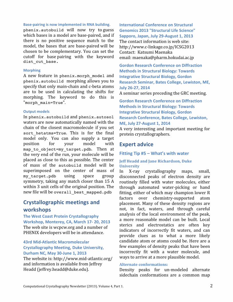
feature that may be erroneously filled with water molecules. In Fig. 1 (left panel), Asp 9 of 1EB6 is fit as a t70 rotamer. The two nearby waters are reasonable fits to their respective density peaks, but both have significant steric clashes with the hydrophobic C-‐beta hydrogen. Rather than two waters, an alternate conformation for Asp A 9 in an m-‐20 rotamer fits the two density peaks very well (right panel), and is sterically viable. Note that the backbone must be altered slightly to accommodate the m-‐20 alternate through a

6

“backrub” motion (Davis 2006), as discussed in Fitting Tip #4 in CCN, July, 2012.

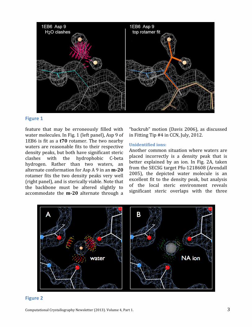
Unidentified ions: Another common situation where waters are placed incorrectly is a density peak that is better explained by an ion. In Fig. 2A, taken from the SECSG target Pfu-‐1218608 (Arendall 2005), the depicted water molecule is an excellent fit to the density peak, but analysis of the local steric environment reveals significant steric overlaps with the three

Figure 1

Figure 2


7

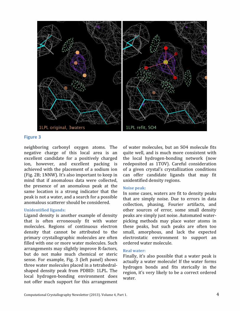
neighboring carbonyl oxygen atoms. The negative charge of this local area is an excellent candidate for a positively charged ion, however, and excellent packing is achieved with the placement of a sodium ion (Fig. 2B; 1NNW). It’s also important to keep in mind that if anomalous data were collected, the presence of an anomalous peak at the same location is a strong indicator that the peak is not a water, and a search for a possible anomalous scatterer should be considered. Unidentified ligands: Ligand density is another example of density that is often erroneously fit with water molecules. Regions of continuous electron density that cannot be attributed to the primary crystallographic molecules are often filled with one or more water molecules. Such arrangements may slightly improve R-‐factors, but do not make much chemical or steric sense. For example, Fig. 3 (left panel) shows three water molecules placed in a tetrahedral-‐shaped density peak from PDBID: 1LPL. The local hydrogen-‐bonding environment does not offer much support for this arrangement

Figure 3

8

of water molecules, but an SO4 molecule fits quite well, and is much more consistent with the local hydrogen-‐bonding network (now redeposited as 1TOV). Careful consideration of a given crystal’s crystallization conditions can offer candidate ligands that may fit unidentified density regions. Noise peak: In some cases, waters are fit to density peaks that are simply noise. Due to errors in data collection, phasing, Fourier artifacts, and other sources of error, some small density peaks are simply just noise. Automated water-‐picking methods may place water atoms in these peaks, but such peaks are often too small, amorphous, and lack the expected electrostatic environment to support an ordered water molecule. Real water: Finally, it’s also possible that a water peak is actually a water molecule! If the water forms hydrogen bonds and fits sterically in the region, it’s very likely to be a correct ordered water.


9

Future development: To supplement the water picking method in phenix.refine, automatic identification and building of other structural features (alternate conformations, ligands, etc.) is an active focus of Phenix development. Ion placement will be available in the near future. References: Davis IW, Arendall WB III, Richardson JS, Richardson DC (2006). "The backrub motion: How protein backbone shrugs when a sidechain dances" Structure 14:265-‐274.

Arendall WB III, Tempel W, Richardson JS, Zhou W, Wang S, Davis IW, Liu Z-‐J, Rose JP, Carson WM, Luo M, Richardson DC, Wang B-‐C (2005). "A test of enhancing model accuracy in high-‐throughput crystallography." Journal of Structural and Functional Genomics 6:1-‐11.

10

Contributors P. D. Adams, H. M. Berman, G. Bunkóczi, V. B. Chen, L. N. Deis, N. Echols, M. J. Gabanyi, L. K. Gifford, R. J. Gildea, R. W. Grosse-‐Kunstleve, J. J. Headd, N. W. Moriarty, M. H. Prisant, D. C. Richardson, J. S. Richardson, J. Snoevink, T. C. Terwilliger, V. Verma, L. L. Videau

FAQ This issue’s FAQ grow to such an extent that it merits its own section. See next page.

6

frequently Asked Questions

Computational Crystallography Newsletter (2013). 4, 6–8

1

I'm seeing a lot of CIF files. Are they all restraints? Richard J. Gildeaa, Nigel W. Moriartya and Paul D. Adamsa,b

aLawrence Berkeley National Laboratory, Berkeley, CA 94720 bDepartment of Bioengineering, University of California at Berkeley, Berkeley, CA 94720

Correspondence email: [email protected]

2

Introduction The acronym CIF is used both to refer to the Crystallographic Information File1, and the Crystallographic Information Framework. CIF is designed to be a human and machine-‐readable text format consisting of pairs of data names and data items (with a looping facility that allows repeated items). The IUCr maintains a central repository of application-‐specific machine-‐readable CIF dictionaries, containing a collection of standard data names along with definitions and permissible values. The formal specification of the CIF format and data name dictionaries can be found at the IUCr website2. The macromolecular CIF dictionary (mmCIF) contains those data names that are necessary to describe the results of a macromolecular crystallographic experiment.

As a flexible and extensible format, CIF is used to record a variety of information in different contexts. Phenix3 programs are capable of reading and writing several different types of CIF files. Here we present a summary of the various types of CIF file that the typical user of a macromolecular refinement program may encounter.

Restraint files Restraint CIF files contain the minimum information necessary for a refinement program to restrain the internal coordinates of a given monomer to chemically meaningful values. The CCP4 monomer library4 and the GeoStd5 contain a complete description of the internal chemical structure for the most common monomers, including ideal target values for bonds, angles and torsion angles, and also definitions of planarity and chirality if required.

3

Both libraries also contain other pieces of useful information including common residue synonyms and common links such as the bonds for inter-‐residue restraints. In addition, the GeoStd contains the rotamer information for the common amino acids.

Generation of restraint files in Phenix is handled by eLBOW6, which is called by a number of other programs including ReadySet! and the ligand pipeline.

Chemical components files The PDB chemical components dictionary7 describes all monomers and small molecule components found in PDB entries. Each chemical component entry is referenced by the 3-‐character alphanumeric code assigned to it by the PDB, and contains detailed chemical information and idealized coordinates. Chemical components files can be used as input to phenix.elbow in order to generate restraints (in CIF format) for refinement. A chemical components file may look superficially similar to a restraints file, however it lacks the necessary information on target values for restraints that is needed by the refinement program.

Coordinate files Currently, the PDB format8 is the most widely used file format for storing the atom site coordinates of macromolecular structures. Alternatively, it is possible to record the atom site coordinates (and much more) in CIF format files, with both formats accepted for PDB deposition. The atomic coordinates in both PDB and CIF files can be obtained from the PDB database using the command

phenix.fetch_pdb 1xxx --all

7 Computational Crystallography Newsletter (2013). 4, 6–8

Frequently asked questions

4

This will download the following files:

Coordinate CIF files can be identified by the presence of the atom_site loop containing information about the atom sites, similar to that stored in the PDB ATOM record: element type, Cartesian or fractional site coordinates, atomic B-‐factor, occupancy, atom name, residue name, alternate location identifier, residue sequence number, insertion code, chain ID, etc. Look for the presence of a section that looks something like this (the order and exact data items present may vary depending on the source of the file):

loop_ _atom_site.group_PDB _atom_site.id _atom_site.label_atom_id _atom_site.label_alt_id _atom_site.label_comp_id _atom_site.auth_asym_id _atom_site.auth_seq_id _atom_site.pdbx_PDB_ins_code _atom_site.Cartn_x _atom_site.Cartn_y _atom_site.Cartn_z _atom_site.occupancy _atom_site.B_iso_or_equiv _atom_site.type_symbol _atom_site.pdbx_formal_charge _atom_site.label_asym_id _atom_site.label_entity_id _atom_site.label_seq_id _atom_site.pdbx_PDB_model_num Coordinate CIF files typically also contain a description of the unit cell and crystallographic symmetry. Frequently, they also describe experimental details, similar to those present in the PDB REMARK records, but presented in a much more computer-‐readable format. Coordinate mmCIF files can now be used in place of PDB-‐format coordinate files in most Phenix programs (e.g. phenix.refine9, phenix.model_vs_data10), and phenix.refine will output the coordinates in CIF format given the option write_model_cif_file=True.

5

Reflection data files Users of reflection data from the PDB will be familiar with the mmCIF format reflection files, most probably as an additional step where they need to first convert the reflection data to MTZ format, e.g. using phenix.cif_as_mtz, before being able to use the reflection data with their favorite programs. For some time, Phenix has supported the direct use of mmCIF format reflection files in place of MTZ files in many programs, although it may still be preferable to use an MTZ file for normal workflow, as the binary MTZ file format is inherently faster for file reading, particularly for large datasets. phenix.refine will output the reflections in CIF format given the option write_reflection_cif_file=True. An mmCIF format reflection file will contain a section similar to this:

loop_ _refln.index_h _refln.index_k _refln.index_l _refln.F_meas_au _refln.F_meas_sigma_au _refln.pdbx_FWT _refln.pdbx_PHWT _refln.pdbx_DELFWT _refln.pdbx_DELPHWT _refln.status Depending on the source of the file and the type of reflection data contained, the order and exact items present may vary, however the columns containing the miller indices, _refln.index_h, etc., must be present.

Small molecule CIF files Coordinate and reflection data files obtained from the Cambridge Structural Database (CSD) or the Crystallography Open Database (COD) may look similar to the files described above, however these files use a slightly different set of data names based on an older version of the dictionary definition language (DDL) that describes the relationships between data names. Small molecule CIF files are not currently utilized by any Phenix program.

1xxx.pdb (atomic coordinates in PDB format) 1xxx.cif (atomic coordinates in CIF format) 1xxx-sf.cif (reflection data in CIF format) 1xxx.fa (sequence file in FASTA format)


Frequently asked questions

6

References 1S. R. Hall, F. H. Allen and I. D. Brown, Acta Cryst. (1991). A47, 655-‐685 2http://www.iucr.org/resources/cif 3P. D. Adams, P. V. Afonine, G. Bunkóczi, V. B. Chen, I. W. Davis, N. Echols, J. J. Headd, L.-‐W. Hung, G. J. Kapral, R. W. Grosse-‐Kunstleve, A. J. McCoy, N. W. Moriarty, R. Oeffner, R. J. Read, D. C. Richardson, J. S. Richardson, T. C. Terwilliger and P. H. Zwart (2010). Acta Cryst. D66, 213-‐221. 4A. A. Vagin, R. A. Steiner, A. A. Lebedev, L. Potterton, S. McNicholas, F. Long and G. N. Murshudov, (2004). Acta Cryst. D60, 2184-‐2195. 5http://geostd.sourceforge.net/ 6N. W. Moriarty, R. W. Grosse-‐Kunstleve and P. D. Adams, Acta Cryst. (2009). D65, 1074-‐1080. 7http://www.wwpdb.org/ccd.html 8http://www.wwpdb.org/documentation/format33/v3.3.html 9P. V. Afonine, R. W. Grosse-‐Kunstleve, N. Echols, J. J. Headd, N. W. Moriarty, M. Mustyakimov, T. C. Terwilliger, A. Urzhumtsev, P. H. Zwart and P. D. Adams. Acta Cryst. 2012,D68:352-‐367 10P. V. Afonine, R. W. Grosse-‐Kunstleve, V. B. Chen, J. J. Headd, N. W. Moriarty, J. S. Richardson, D. C. Richardson, A. Urzhumtsev, P. H. Zwart and P. D. Adams. J. Appl. Cryst. (2010). 43, 669-‐676.

9

9

SHORT COMMUNICATIONS


1

Phenix / MolProbity Hydrogen Parameter Update Lindsay N. Deisa, Vishal Vermab, Lizbeth L. Videaua, Michael G. Prisanta, Nigel W. Moriartyc, Jeffrey J. Headda, Vincent B. Chena, Paul D. Adamsc,d, Jack Snoeyinkb, Jane S. Richardsona, and David C. Richardsona

aDuke University, Durham, NC bUniversity of North Carolina, Durham, NC cLawrence Berkeley National Laboratory, Berkeley, CA dBioengineering Department, University of California Berkeley, Berkeley, CA


2

The new distribution of PHENIX incorporates major updates in the parameters and procedures for hydrogen atoms, providing consistency between phenix.refine and MOLPROBITY and more correct treatment in each system across the range of usage needs.

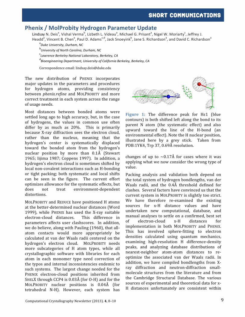
Most distances between bonded atoms were settled long ago to high accuracy, but, in the case of hydrogens, the values in common use often differ by as much as 20%. This is primarily because X-‐ray diffraction sees the electron cloud, rather than the nucleus, meaning that the hydrogen’s center is systematically displaced toward the bonded atom from the hydrogen’s nuclear position by more than 0.1Å (Stewart 1965; Iijima 1987; Coppens 1997). In addition, a hydrogen's electron cloud is sometimes shifted by local non-‐covalent interactions such as H-‐bonding or tight packing; both systematic and local shifts can be seen in the figure. The current effort optimizes allowance for the systematic effects, but does not treat environment-‐dependent distortions.

MOLPROBITY and REDUCE have positioned H atoms at the better-‐determined nuclear distances (Word 1999), while PHENIX has used the X-‐ray suitable electron-‐cloud distances. This difference in parameters affects user clashscores. In addition, we do believe, along with Pauling (1960), that all-‐atom contacts would more appropriately be calculated at van der Waals radii centered on the hydrogen's electron cloud. MOLPROBITY needs more subcategories of H atom types, while all crystallographic software with libraries for each atom in each monomer type need correction of the typos and internal inconsistencies endemic to such systems. The largest change needed for the PHENIX electron-‐cloud positions inherited from SHELX through CCP4 is 0.03Å (for O-‐H) and for the MOLPROBITY nuclear positions is 0.04Å (for tetrahedral N-‐H). However, each system has

3

changes of up to ~0.17Å for cases where it was applying what we now consider the wrong type of value.

Packing analysis and validation both depend on the total system of hydrogen bondlengths, van der Waals radii, and the 0.4Å threshold defined for clashes. Several factors have convinced us that the current system in MOLPROBITY is slightly too strict. We have therefore re-‐examined the existing sources for x-‐H distance values and have undertaken new computational, database, and manual analyses to settle on a confirmed, best set of electron-‐cloud x-‐H distances for implementation in both MOLPROBITY and PHENIX. This has involved sphere-‐fitting to electron densities calculated using quantum mechanics, examining high-‐resolution H difference-‐density peaks, and analyzing database distributions of nearest-‐neighbor atom-‐atom distances to re-‐optimize the associated van der Waals radii. In addition, we have compiled bondlengths from X-‐ray diffraction and neutron-‐diffraction small-‐molecule structures from the literature and from the Cambridge Structural Database. The various sources of experimental and theoretical data for x-‐H distances unfortunately are consistent within

Figure 1: The difference peak for Hε1 (blue contours) is both shifted left along the bond to its parent N atom (the systematic effect) and also upward toward the line of the H-‐bond (an environmental effect). Note the H nuclear position, illustrated here by a grey stick. Taken from PDB:1YK4, Trp 37, 0.69Å resolution.


SHORT Communications

4

0.01Å only for the nuclear aliphatic C-‐H case, so that future research would still be desirable. However, we judge that the values presented here are correct within 0.02-‐0.03Å, nearly an order of magnitude better than the previous situation. Happily, we find that the new parameters produce clashscores that have a better trend towards zero for the best structures at mid to high resolutions and do a slightly better job determining sidechain NQH flips.

We are currently implementing this change in both MOLPROBITY and PHENIX so that the two

5

services will add hydrogens identically and in an appropriately application-‐specific fashion. The electron-‐cloud values will be the default in both systems due to the predominant use for X-‐ray crystallography. However, each will also include an option to use updated nuclear positions for neutron-‐diffraction refinement, for NMR structures, or by user choice, and MOLPROBITY will use van der Waals radii tuned for each case when calculating all-‐atom contacts.

6

References Coppens P (1997) X-‐ray Charge Densities and Chemical Bonding, Oxford University Press, NY, ISBN 0-‐19-‐

509823-‐4. Iijima H, Dunbar JBJ, Marshall GR (1987) Calibration of effective van der Waals atomic contact radii for

proteins and peptides. Proteins: Struct. Funct. Genet. 2: 330-‐339. Pauling L (1960) The Nature of the Chemical Bond, 3rd ed, Cornell University Press, Ithaca, ISBN 0-‐8014-‐

0333-‐2. Stewart RF, Davidson ER, Simpson WT (1965) Coherent x-‐ray scattering for the hydrogen atom in the

hydrogen molecule, J. Chem. Phys. 42: 3175-‐87. Word JM, Lovell SC, LaBean TH, et al. (1999) Visualizing and quantifying molecular goodness-‐of-‐fit:

Small-‐probe contact dots with explicit hydrogen atoms, J. Mol. Biol. 285: 1711-‐33.



1

PSI SBKB Technology Portal: A Web Resource for Structural Biologists Lida K. Gifforda, Margaret J. Gabanyib, Helen M. Bermanb, and Paul D. Adamsa

aPhysical Biosciences Division, Lawrence Berkeley National Laboratory, Berkeley, CA 94720. bDepartment of Chemistry & Chemical Biology, Rutgers – The State University of New Jersey, Piscataway, NJ 08854.


2

Introduction The Protein Structure Initiative (PSI) was first funded in 2000 and remains committed to facilitating the process of solving three-‐dimensional atomic-‐level protein structures [1]. In 2008, a web-‐based resource, now the Structural Biology Knowledgebase (SBKB, sbkb.org), was established to capture and disseminate structural data and results from PSI research [2]. The Knowledgebase has a modular architecture providing access to individual websites for experimental data tracking, protocols, materials, protein annotations, modeling, technologies, and publications. It also makes connections to related data found in GO [3], PDB [4], UniProt [5], and 100+ other publicly available gene and protein resources.

The Technology Portal is one module of the SBKB and is designed to present methods and technologies catalyzed by the PSI high-‐throughput protein production and structure determination efforts [6]. In addition, it functions as a repository for tools developed by the wider scientific community for structural biologists to take and use in their research. An overarching goal of the Technology Portal is to encourage collaboration among scientists, not only within the PSI, but also between PSI researchers and the broader biological community.

This web resource is comprised of 350 tools and technology summaries representing each step of the protein structure determination pipeline, the majority of which have been developed by the PSI and are in use at PSI Centers. The Technology Portal home page presents all items in one easy-‐to-‐navigate page. While several components of the Portal have been described in-‐depth elsewhere [6], an overview of the search functionality and accessible tools will be presented, with particular emphasis placed on new features.

3

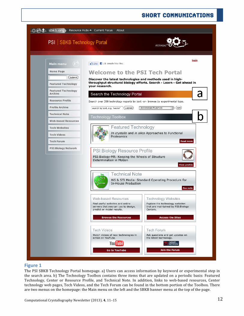
The Technology Portal Website The Technology Portal can be reached directly (technology.sbkb.org/portal/) or via the Methods Hub of the SBKB (sbkb.org/kb/methodshub.html). In addition, performing a keyword search on the SBKB can access Technology Portal information. Once at the Portal homepage, users can access all of its technology pages and online resources. The Technology Portal is hosted using Apache HTTP software [7] and constructed using the Django 1.2 web framework [8], which accesses data from a SQLite 3 database [9] and presents them as technology pages. A screen shot of the current homepage shows all of the content and functionalities (Figure 1).

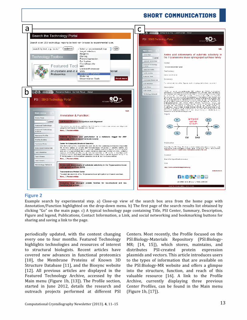
Searching the Technology Portal There are two ways to search technologies from the Technology Portal homepage: plain text and by experimental stage (Figure 2a). A text search box will return a list of technology pages with the most recently edited pages shown first, prioritizing technology pages containing the newest information. Each technology is indexed by step in the structure determination process, so a more general search can be performed by choosing one of the following topics from a drop-‐down menu: Target Selection, Reagents, Cloning, Protein Expression, Purification, Crystallography, NMR, Electron Microscopy, SAXS, Annotation/Function, Modeling, or Dissemination Tools. Users can browse search results, which are presented in an alphabetical listing of all records tagged for that particular process (Figure 2b). Technology pages contain all pertinent information, such as a description of the technology, figures, and information regarding publication, whom to contact, web links, and availability, if applicable (Figure 2c).

Technology Toolbox The first items listed in the Technology Toolbox are the Featured Technology article, Profile, and Technical Note (Figure 1a). All of these features are



Figure 1 The PSI SBKB Technology Portal homepage. a) Users can access information by keyword or experimental step in the search area. b) The Technology Toolbox contains three items that are updated on a periodic basis: Featured Technology, Center or Resource Profile, and Technical Note. In addition, links to web-‐based resources, Center technology web pages, Tech Videos, and the Tech Forum can be found in the bottom portion of the Toolbox. There are two menus on the homepage: the Main menu on the left and the SBKB banner menu at the top of the page.



4

periodically updated, with the content changing every one to four months. Featured Technology highlights technologies and resources of interest to structural biologists. Recent articles have covered new advances in functional proteomics [10], the Membrane Proteins of Known 3D Structure Database [11], and the Biosync website [12]. All previous articles are displayed in the Featured Technology Archive, accessed by the Main menu (Figure 1b, [13]). The Profile section, started in June 2012, details the research and outreach projects performed at different PSI

5

Centers. Most recently, the Profile focused on the PSI:Biology-‐Materials Repository (PSI:Biology-‐MR; [14, 15]), which stores, maintains, and distributes PSI-‐created protein expression plasmids and vectors. This article introduces users to the types of information that are available on the PSI:Biology-‐MR website and offers a glimpse into the structure, function, and reach of this valuable resource [16]. A link to the Profile Archive, currently displaying three previous Center Profiles, can be found in the Main menu (Figure 1b, [17]).

Figure 2 Example search by experimental step. a) Close-‐up view of the search box area from the home page with Annotation/Function highlighted on the drop-‐down menu. b) The first page of the search results list obtained by clicking “Go” on the main page. c) A typical technology page containing Title, PSI Center, Summary, Description, Figure and legend, Publications, Contact Information, a Link, and social networking and bookmarking buttons for sharing and saving a link to the page.



6

The most recent addition to the Technology Toolbox is the Technical Note. This feature was established in December 2012 and the inaugural entry describes the standard operating procedure for making insect cell media in-‐house [18], contributed by James D. Love, PhD, Head of Technology, New York Structural Genomics Research Consortium (nysgrc.org). This Note will change periodically and be used to disseminate detailed protocols that would be beneficial to a wide audience of structural biologists.

The bottom portion of the Technology Toolbox contains links to Web-‐based Resources, Tech Websites, Tech Videos, and the Tech Forum. The Web-‐Related Resources section contains a list of over 70 technology pages describing web servers or web-‐based tools that can be employed by structural biologists to design, predict, and model results (technology.sbkb.org/portal/useful_servers). Clicking on Tech Websites takes users to a page listing the technology websites maintained by PSI Centers. All four of the PSI:Biology High-‐Throughput Centers for Protein Structure Determination, over half of the Centers for Membrane Protein Structure Determination, and the Mitochondrial Protein Partnership, a PSI:Biology Consortium for High-‐Throughput Enabled Structural Biology Partnership, maintain web pages describing the software, tools, and other technologies they have developed to relieve bottlenecks in protein structure determination (technology.sbkb.org/portal/technology_links). The Tech Videos page displays sbkbtech YouTube channel videos (www.youtube.com/user/sbkbtech). Currently, there are eight technologies in action (technology.sbkb.org/portal/video). Tech Forum is a direct conduit to the Technology Portal Forum group (network.nature.com/groups/psikb_tech/) hosted on the Nature Network. This forum provides a virtual place for scientists to connect on a professional level and exchange information about structural biology technology.

Outreach The Technology Portal maintains a Facebook page at facebook.com/techportal. Posting of new content is announced on Facebook, as well as interesting items from the SBKB [19] and PSI:Biology-‐MR [20] Facebook pages, meeting announcements, and notifications from sources such as Nature [21], the Protein Data Bank [4], and NCBI [22].

7

The Technology Portal works closely with two other PSI:Biology web resources by using link-‐outs to connect useful information between sites. For example, the PSI Publications Portal (olenka.med.virginia.edu/psi/) contains all publication information and statistics for the more than 1800 peer-‐reviewed articles that have been published by the PSI over the past 12 years. Users can find links to article summaries on most technology pages. In addition, if a publication is referenced on a technology page, the Publications Portal entry contains a link to the appropriate page on the Technology Portal.

Crosslinks have also been established with the PSI:Biology-‐Materials Repository (psimr.asu.edu/; [14, 15]). All technology pages describing a vector designed and used by PSI Centers contain availability information and a link to the PSI:Biology-‐MR. Reciprocally, on appropriate vector pages, the PSI:Biology-‐MR refers users to the Technology Portal for more information.

Conclusion The Technology Portal is dedicated to capturing and highlighting technological advances that are instrumental to enabling structural biological research. This is accomplished by collaborating with PSI Centers and members of the wider scientific community to gather methods and tools that have been developed that would be widely beneficial to scientists. Tech Portal feature articles and technology pages are updated frequently so that scientists can take and use the knowledge and tools provided in their research. We welcome feedback from the community at psi-‐[email protected].

Acknowledgements The authors would like to thank the Protein Structure Initiative PIs, researchers, and Structural Biology Knowledgebase members for their collaboration and support of the Technology Portal. We thank Nicholas Sauter for server maintenance and technical support. The Technology Portal is a resource center within the Protein Structure Initiative and is supported by grant U01GM093324 from the National Institute of General Medical Sciences. This work was supported in part by the US Department of Energy under Contract No. DE-‐AC02-‐05CH11231.



8

References 1. Gabanyi MJ, et al. (2011) The Structural Biology Knowledgebase: a portal to protein structures,

sequences, functions, and methods. J Struct Funct Genomics 12(2):45-‐54. 2. Berman HM, et al. (2009) The Protein Structure Initiative Structural Genomics Knowledgebase.

Nucleic Acids Res 37(Database issue):D365-‐368. 3. The Gene Ontology Consortium. (2000) Gene Ontology: tool for the unification of biology. Nature

Genet. 25:25-‐29. 4. Berman HM, et al. (2000) The Protein Data Bank. Nucleic Acids Res 28:235-‐242. 5. The UniProt Consortium. (2012) Reorganizing the protein space at the Universal Protein Resource

(UniProt). Nucleic Acids Res 40:D71-‐D75. 6. Gifford LK, Carter LG, Gabanyi MJ, Berman HM, & Adams PD. (2012) The Protein Structure Initiative

Structural Biology Knowledgebase Technology Portal: a structural biology web resource. J Struct Funct Genomics 13(2):57-‐62.

7. Apache HTTP Server Project. (2011) Available from: http://httpd.apache.org/ 8. Django: A Python Web Framework. (2005) Available from: http://www.djangoproject.com 9. SQLite 3: SQL database engine. (2004) Available from: http://www.sqlite.org/ 10. PSI SBKB Technology Portal. (2012) In crystallo and in silico Approaches to Functional Proteomics.

Available from: http://technology.sbkb.org/portal/fall_2012_feat_tech 11. White, S. (1998) Membrane Proteins of Known 3D Structure Database. Available from:

http://blanco.biomol.uci.edu/mpstruc/ 12. Kuller A, et al. (2002) A biologist's guide to synchrotron facilities: the BioSync web resource. Trends

Biochem Sci 27(4):213-‐215. 13. PSI SBKB Technology Portal. (2011) PSI Tech Portal Featured Technology Archive. Available from:

http://technology.sbkb.org/portal/archive 14. Cormier CY, et al. (2010) Protein Structure Initiative Material Repository: an open shared public

resource of structural genomics plasmids for the biological community. Nucleic Acids Res 38(Database issue):D743-‐749.

15. Cormier CY, et al. (2011) PSI:Biology-‐materials repository: a biologist's resource for protein expression plasmids. J Struct Funct Genomics 12(2):55-‐62.

16. PSI SBKB Technology Portal. (2012) PSI:Biology-‐Materials Repository: Keeping the Wheels of Structure Determination in Motion. Available from: http://technology.sbkb.org/portal/PSIMR_profile

17. PSI SBKB Technology Portal. (2012) PSI Tech Portal Profile Archive. Available from: http://technology.sbkb.org/portal/profile_archive

18. PSI SBKB Technology Portal. (2012) Hi5 & Sf9 Media: Standard Operating Procedure for In-‐House Production. Available from: http://technology.sbkb.org/portal/insect_tech_note

19. PSI Structural Biology Knowledgebase. (2010) PSI Structural Biology Knowledgebase Facebook Page. Available from: https://www.facebook.com/psisbkb

20. PSI:Biology-‐Materials Repository. (2010) PSI:Biology-‐Materials Repository (PSI:Biology-‐MR) Facebook Page. Available from: https://www.facebook.com/pages/PSIBiology-‐Materials-‐Repository-‐PSIBiology-‐MR/108495809177357

21. Nature Publishing Group. (2007) Nature Facebook Page. Available from: https://www.facebook.com/nature

22. National Center for Biotechnology Information. (2010) NCBI -‐ National Center for Biotechnology Information Facebook Page. Available from: https://www.facebook.com/ncbi.nlm

16

ARTICLES


1

cctbx tools for transparent parallel job execution in Python. I. Foundations Gábor Bunkóczia and Nathaniel Echolsb

aDepartment of Haematology, University of Cambridge, Cambridge, UK bLawrence Berkeley National Laboratory, Berkeley, CA


2

Introduction Parallelization can distribute independent calculations over multiple processing units and can decrease the run time of a series of slow calculations. Unfortunately, parallel code is also more complicated, therefore error-‐prone and difficult to maintain. While there are several reasons for increased complexity, notably the need for synchronization between parallel processes, maintenance of parallel-‐enabled program sections is also a (perhaps underrated) problem that deserves attention.

While most languages do not provide direct support for parallelization and rely on low-‐level operating system support, there are successful initiatives for enabling parallel processing either by compiler technology (e.g. OpenMP, http://openmp.org) or an external library component (e.g. Intel Threading Building Blocks, http://threadingbuldingblocks.org). Similarly, the Python-‐specific scheduling module (Bunkóczi & Echols, 2012) provides high-‐level constructs for transparent parallel execution that aim to be minimally intrusive on code layout. It is available with the libtbx module of the Computational Crystallography Toolbox (cctbx, http://cctbx.sourceforge.net; Grosse-‐Kunstleve et al., 2002), the open-‐source component of the PHENIX project (http://www.phenix-‐online.org; Adams et al., 2010).

Problem setting For the purposes of this article, parallelization is defined as multiple simultaneous job execution managed at Python code level. This includes the Python standard library modules threading and multiprocessing, as well as any module that supports job execution on batch queue systems (e.g. libtbx.queuing_system_utils.processing), as long as they provide a factory function that conforms to a standard interface defined by threading.Thread or multiprocessing.Process. Parallelization technologies that affect code at lower levels (e.g. an

3

OpenMP-‐parallelized function exported to Python) are excluded from the discussion.

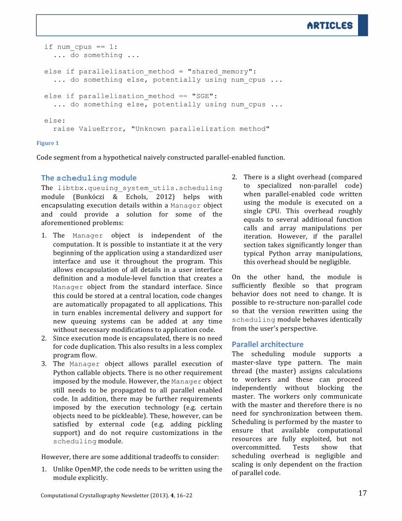
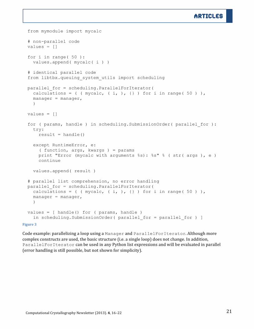
A typical maintenance problem is illustrated with the (slightly exaggerated) code example on Figure 1. Apart from not being aesthetically pleasing, there are several serious problems with this pattern:

1. It is not feasible to come up with a (sufficiently) comprehensive list of all possible parallelization techniques, especially batch queue managers. New systems may appear in the future, or may become non-‐backwards compatible after a major release. In this case, the existing codebase has to be searched and amended as necessary.

2. There exist almost certainly instances of severe code duplication among the branches of the conditional expression. If the algorithm changes, all branches need to be updated. Moreover, the algorithm logic is potentially interleaved with calculation details and it is more difficult to follow the program flow.

3. The program will typically contain several parallel sections and parameters of parallel execution to be propagated to all of these. In addition to distributing knowledge throughout the program (discussed in 1), this makes it very difficult or impossible to reuse existing parts, because parallelization normally lies outside the computational domain of a given calculation. This requires the introduction of numerous thin wrappers and further code duplication, because details of parallelization are not mandated to be universal among different programs and are therefore potentially incompatible.


ARTICLES

4

The scheduling module The libtbx.queuing_system_utils.scheduling module (Bunkóczi & Echols, 2012) helps with encapsulating execution details within a Manager object and could provide a solution for some of the aforementioned problems:

1. The Manager object is independent of the computation. It is possible to instantiate it at the very beginning of the application using a standardized user interface and use it throughout the program. This allows encapsulation of all details in a user interface definition and a module-‐level function that creates a Manager object from the standard interface. Since this could be stored at a central location, code changes are automatically propagated to all applications. This in turn enables incremental delivery and support for new queuing systems can be added at any time without necessary modifications to application code.

2. Since execution mode is encapsulated, there is no need for code duplication. This also results in a less complex program flow.

3. The Manager object allows parallel execution of Python callable objects. There is no other requirement imposed by the module. However, the Manager object still needs to be propagated to all parallel enabled code. In addition, there may be further requirements imposed by the execution technology (e.g. certain objects need to be pickleable). These, however, can be satisfied by external code (e.g. adding pickling support) and do not require customizations in the scheduling module.

However, there are some additional tradeoffs to consider:

1. Unlike OpenMP, the code needs to be written using the module explicitly.

5

2. There is a slight overhead (compared to specialized non-‐parallel code) when parallel-‐enabled code written using the module is executed on a single CPU. This overhead roughly equals to several additional function calls and array manipulations per iteration. However, if the parallel section takes significantly longer than typical Python array manipulations, this overhead should be negligible.

On the other hand, the module is sufficiently flexible so that program behavior does not need to change. It is possible to re-‐structure non-‐parallel code so that the version rewritten using the scheduling module behaves identically from the user's perspective.

Parallel architecture The scheduling module supports a master-‐slave type pattern. The main thread (the master) assigns calculations to workers and these can proceed independently without blocking the master. The workers only communicate with the master and therefore there is no need for synchronization between them. Scheduling is performed by the master to ensure that available computational resources are fully exploited, but not overcommitted. Tests show that scheduling overhead is negligible and scaling is only dependent on the fraction of parallel code.

if num_cpus == 1: ... do something ...

else if parallelisation_method = "shared_memory":

... do something else, potentially using num_cpus ... else if parallelisation_method == "SGE":

... do something else, potentially using num_cpus ... else: raise ValueError, "Unknown parallelization method"

Figure 1

Code segment from a hypothetical naively constructed parallel-‐enabled function.


ARTICLES

6

The scheduler component is provided by implementations of the Manager interface. Calculations that can be delegated to workers take the form of Python function calls, with a callable (either function or method) and (positional and keyword) arguments. These are stored inside the Manager object and the calculation is started when a worker becomes idle. Calculation status queries and access to results are made available through method calls.

Manager models The Manager interface is an abstraction for controlling program behavior from the users' perspective. It is defined in the scheduling module and allows multiple implementations with varying properties so that a good match for the program's requirements could either be found or implemented. There are currently three basic implementations available:

• Manager. This has possibly the most widespread applicability. It manages not only the execution of calculations (which is pre-‐configured, but allowed to be a mixture of modes), but also a job queue. It assumes, however, that executing a calculation does not block the main thread of control.

• MainthreadManager. This is a dummy Manager that executes calculations on the main thread. Execution is delayed so that output can keep scrolling as calculations complete. In addition, this has the lowest job startup overhead equivalent to about a single function call and is therefore the right choice if there is only one processing unit available.

• Adapter. This allows sharing of a single Manager instance in order to provide scalable computing power to multiple parts of the same application. It behaves as a Manager with a variable number of processing units, since depending on resource utilization of other components, computational resources available to a given component can vary.

There are additional classes that may be necessary for certain tasks and whose implementations are pending:

• QueueManager. This implements access to a batch queuing system and delegates queue management to the same. Only a single

7

execution mode is allowed, but the number of concurrent processes is unlimited.

• PoolManager. Instead of creating a new thread of control for each calculation, this re-‐uses a pre-‐created pool of workers. If running through a batch queue system, this could lower job startup overhead considerably as it would effectively bypass the job queue. An efficient implementation could also provide for automatic resource allocation/de-‐allocation according to the load.

Calculation results and error handling The Manager is unaware of any backwards communication between the actual workers and their proxies (ExecutionUnits) held by the Manager. This responsibility is handled by the individual ExecutionUnits. After termination of the underlying calculation, the Manager provides an opportunity for the ExecutionUnit to "post-‐process" the results and become ready for accepting the next calculation. In this time window it is possible to obtain results from the worker through a suitable data queue. In case a data queue becomes stuck (e.g. through an NFS latency), the Manager temporarily suspends the ExecutionUnit to avoid stalling the job queue and then periodically retries. Eventually, after a preset timeout, the ExecutionUnit is reset and the calculation is handled as failed.

Signaling error conditions is delayed until the calculation result is accessed. This is to ensure that in case an error occurs the internal state of the Manager is not corrupted, so that processing can be resumed (in case it is allowed by the nature of the computation, e.g. a suitable default value can be substituted for the missing result). The returned job handle is a type with a polymorphic __call__ method that yields the value returned by the call if the job terminated normally or raises a RuntimeError exception if failed. The module currently takes the view that any exception handling code for exceptions that are expected should be included within the call. When executing a call on a batch queue, it is the exit status of the process that is monitored and an error is raised if a process terminates with a non-‐zero exit status. Since execution occurs independently, errors that would normally cause the parent process to terminate if executed on a


ARTICLES

8

separate thread or process (e.g. segmentation fault) can be handled more gracefully, either by logging the error and resuming execution, or by terminating gracefully. A typical error-‐handling scenario is shown in Figure 2.

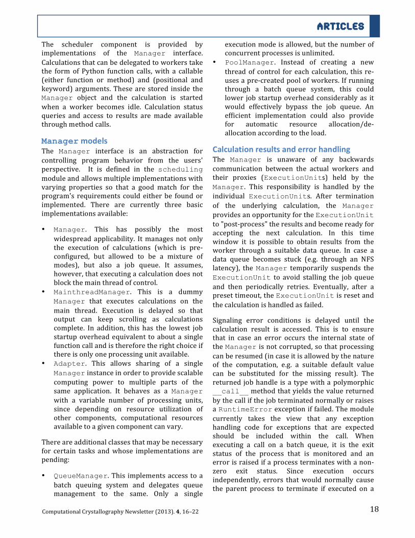
Parallel constructs Using a Manager object directly allows full flexibility. This may be necessary if each job is a different type of calculation or if subsequent jobs are dependent on previously returned results (e.g. from molecular replacement, parallel translation functions for rotation function peaks). The Manager provides an API similar to that of a queuing system. When calls are submitted, the Manager returns a job identifier that can later be used to check whether the job has finished. The Manager also provides various methods to access results of finished calculations. A very simple example is shown in Figure 2.

from mymodule import mycalc identifier1 = manager.submit( target = mycalc, args = ( 1, ) ) identifier2 = manager.submit( target = mycalc, args = ( 2, ) ) # fetch result for designated job handle2 = manager.result_for( identifier = identifier2 ) try:

result2 = handle2() except RuntimeError, e:

print "Second calculation failed" # fetch result for next job handle1 = manager.results.next() try:

result1 = handle1() except RuntimeError, e:

print "First calculation failed"

Figure 2

Code example: using methods of a Manager to submit jobs and wait for results. Manager can return result handles for requested calculations or for the one that finishes next. The __call__ method of a result handle returns immediately and only necessary to signal an error condition. mymodule is a hypothetical module containing the function mycalc. See Bunkóczi & Echols (2012) on how to instantiate a Manager.

9

While having full flexibility is sometimes advantageous, it is not always necessary. In the majority of cases, parallelization is employed to execute a loop in parallel (cf. #pragma omp parallel for). While this can be emulated by an initial for loop that submits all calculations to the Manager, and a subsequent for loop that fetches results for each identifier, this solution suffers from several drawbacks. First, the number of loop iterations is normally larger than the number of available processing units. Input arguments for all calculations have to be generated upfront, unnecessarily filling up memory. Second, there may be a long delay while calculations are being submitted before the result for the first calculation is accessed. This can cause not only user inconvenience, but also accumulation of results that may also lead to out-‐of-‐memory errors. Third, if the sequence of calculations is infinite, the program will never reach the second loop (this may sound rather


ARTICLES

10

esoteric, but it is in fact a valid technique to use an infinite sequence and is employed by several widely used programs in crystallography).

The scheduling module provides the ParallelForIterator class for these situations. This requires a Manager instance and an iterable returning a tuple (target, args, kwargs) that defines each calculation. The ParallelForIterator maps these calculations onto the Manager in a dynamic fashion. Since the iterable can be a generator, the arguments are generated as needed and not upfront. The delay is also much less, because only as many calculations are submitted as there are idle processing units. In addition, processing infinite sequences is possible with finite memory, since calculations are submitted and results are accessed continuously, and at any given time point there is a finite number of active calculations.

In contrast to what is suggested by its name, ParallelForIterator is not a Python iterable. However, an iterable can be constructed by passing the object to the ordering classes FinishingOrder and SubmissionOrder. These control the order in which results are returned. If there is no particular need, FinishingOrder should always be preferred, because it does not incur any memory overhead. SubmissionOrder returns results in the order they appear in the iterable that defines the calculations. However, it can lead to accumulation of results if a calculation finishes much slower then subsequent ones, and may result in an out-‐of-‐memory error (it should be noted that this overhead is unavoidable and not an implementation artifact of SubmissionOrder). On the other hand, a very slow calculation does not represent a bottleneck for execution because

11

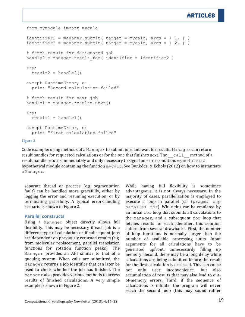
subsequent calculations will be started as soon as ExecutionUnits become idle. Further ordering classes may be developed as needed. A typical example is shown on Figure 3.

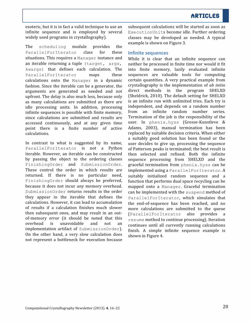
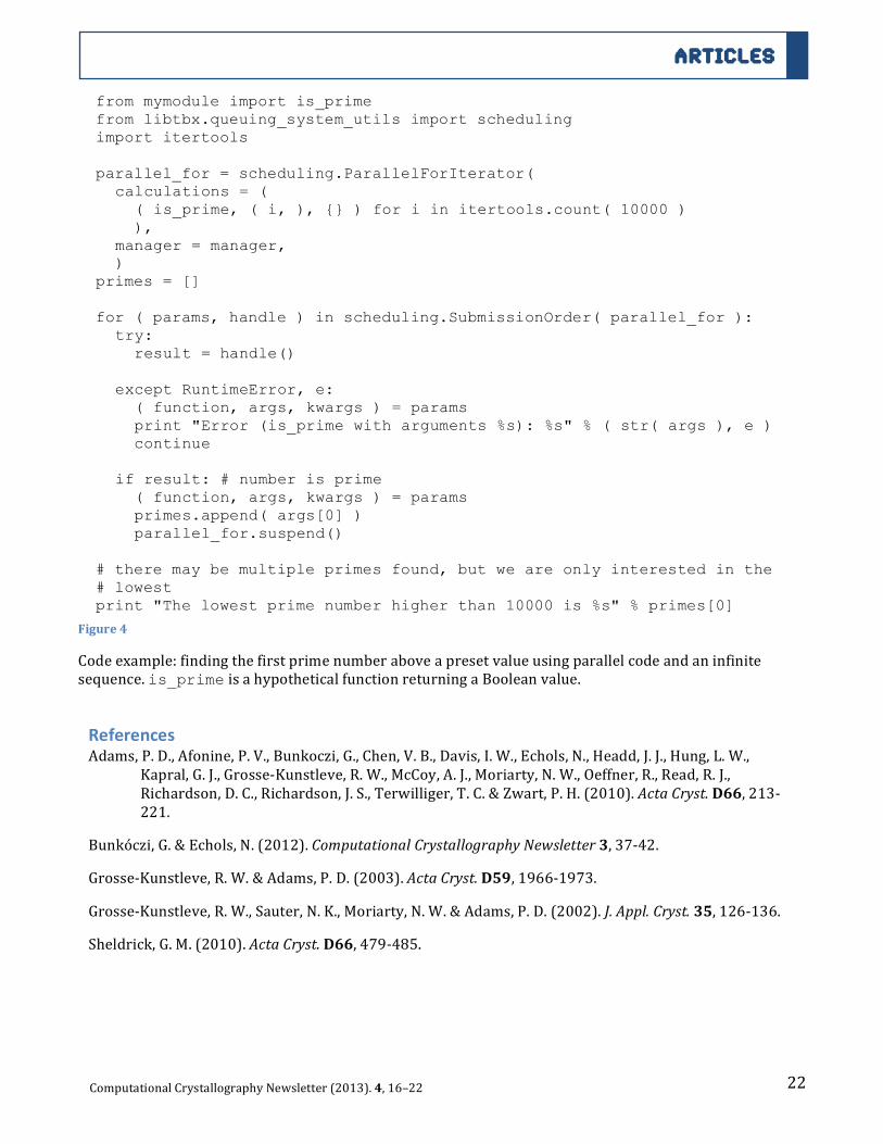
Infinite sequences While it is clear that an infinite sequence can neither be processed in finite time nor would it fit into finite memory, lazily evaluated infinite sequences are valuable tools for computing certain quantities. A very practical example from crystallography is the implementation of ab initio direct methods in the program SHELXD (Sheldrick, 2010). The default setting for SHELXD is an infinite run with unlimited tries. Each try is independent, and depends on a random number from an infinite random number series. Termination of the job is the responsibility of the user. In phenix.hyss (Grosse-‐Kunstleve & Adams, 2003), manual termination has been replaced by suitable decision criteria. When either a suitably good solution has been found or the user decides to give up, processing the sequence of Patterson peaks is terminated; the best result is then selected and refined. Both the infinite sequence processing from SHELXD and the graceful termination from phenix.hyss can be implemented using a ParallelForIterator. A suitably initialized random sequence and a function that performs dual space recycling can be mapped onto a Manager. Graceful termination can be implemented with the suspend method of ParallelForIterator, which simulates that the end-‐of-‐sequence has been reached, and no more calculations are submitted to the queue (ParallelForIterator also provides a resume method to continue processing). Iteration continues until all currently running calculations finish. A simple infinite sequence example is shown in Figure 4.


ARTICLES

from mymodule import mycalc # non-parallel code values = [] for i in range( 50 ): values.append( mycalc( i ) ) # identical parallel code from libtbx.queuing_system_utils import scheduling parallel_for = scheduling.ParallelForIterator(

calculations = ( ( mycalc, ( i, ), {} ) for i in range( 50 ) ), manager = manager, )

values = [] for ( params, handle ) in scheduling.SubmissionOrder( parallel_for ):

try: result = handle() except RuntimeError, e: ( function, args, kwargs ) = params print "Error (mycalc with arguments %s): %s" % ( str( args ), e ) continue values.append( result )

# parallel list comprehension, no error handling parallel_for = scheduling.ParallelForIterator(

calculations = ( ( mycalc, ( i, ), {} ) for i in range( 50 ) ), manager = manager, )

values = [ handle() for ( params, handle ) in scheduling.SubmissionOrder( parallel_for = parallel_for ) ]

Figure 3

Code example: parallelizing a loop using a Manager and ParallelForIterator. Although more complex constructs are used, the basic structure (i.e. a single loop) does not change. In addition, ParallelForIterator can be used in any Python list expressions and will be evaluated in parallel (error handling is still possible, but not shown for simplicity).


ARTICLES

from mymodule import is_prime from libtbx.queuing_system_utils import scheduling import itertools parallel_for = scheduling.ParallelForIterator(

calculations = ( ( is_prime, ( i, ), {} ) for i in itertools.count( 10000 ) ), manager = manager, )

primes = [] for ( params, handle ) in scheduling.SubmissionOrder( parallel_for ):

try: result = handle() except RuntimeError, e: ( function, args, kwargs ) = params print "Error (is_prime with arguments %s): %s" % ( str( args ), e ) continue

if result: # number is prime ( function, args, kwargs ) = params primes.append( args[0] ) parallel_for.suspend()

# there may be multiple primes found, but we are only interested in the # lowest print "The lowest prime number higher than 10000 is %s" % primes[0] Figure 4

Code example: finding the first prime number above a preset value using parallel code and an infinite sequence. is_prime is a hypothetical function returning a Boolean value.

12

References Adams, P. D., Afonine, P. V., Bunkoczi, G., Chen, V. B., Davis, I. W., Echols, N., Headd, J. J., Hung, L. W.,

Kapral, G. J., Grosse-‐Kunstleve, R. W., McCoy, A. J., Moriarty, N. W., Oeffner, R., Read, R. J., Richardson, D. C., Richardson, J. S., Terwilliger, T. C. & Zwart, P. H. (2010). Acta Cryst. D66, 213-‐221.

Bunkóczi, G. & Echols, N. (2012). Computational Crystallography Newsletter 3, 37-‐42.

Grosse-‐Kunstleve, R. W. & Adams, P. D. (2003). Acta Cryst. D59, 1966-‐1973.

Grosse-‐Kunstleve, R. W., Sauter, N. K., Moriarty, N. W. & Adams, P. D. (2002). J. Appl. Cryst. 35, 126-‐136.

Sheldrick, G. M. (2010). Acta Cryst. D66, 479-‐485.


ARTICLES

1

cctbx tools for transparent parallel job execution in Python. II. Convenience functions for the impatient.

Nathaniel Echolsa, Gábor Bunkóczib, and Ralf W. Grosse-‐Kunstlevea,c aLawrence Berkeley National Laboratory, Berkeley, CA bDepartment of Haematology, University of Cambridge, Cambridge, UK cPresent address: Google Inc. (San Bruno, CA)


2

Introduction We have described (Bunkóczi & Echols, 2012, 2013) a set of Python classes for handling parallel execution of tasks on a multiprocessor system or managed cluster. This API has the advantage of being suitable for any situation where parallelism is desired, and is not necessary limited either to “embarrassingly parallel” methods where the same single function is called repeatedly. However, this latter case occurs frequently enough in large applications that it merits its own treatment, and specialized parallelization functions that minimize the programming overhead.

Examples of embarrassingly parallel methods currently used in Phenix (Adams et al., 2010) include:

• Multiple MR searches (phaser.MRage), which were the original motivation for the tools described in the accompanying article

• Multiple Rosetta rebuilding jobs in MR-‐Rosetta (DiMaio et al., 2011)

• Exploration of alternate model-‐building strategies (Terwilliger et al., 2007; Terwilliger, Grosse-‐Kunstleve, Afonine, Moriarty, Zwart, et al., 2008)

• Ligand search trials with varying parameters (Terwilliger et al., 2006)

• Omit map calculation (Terwilliger, Grosse-‐Kunstleve, Afonine, Moriarty, Adams, et al., 2008)

• Optimization of the X-‐ray/restraint weights by grid search in phenix.refine (Afonine et al., 2011; Afonine et al., 2012)

• Validation of multiple models in an ensemble (mmtbx.validation_summary)

Many other crystallographic software packages and automation pipelines employ similar parallelism, including Mr-‐BUMP (Keegan & Winn, 2008), ARCIMBOLDO (Rodriguez et al., 2009; Rodriguez et al., 2012), qFit (van den Bedem et al.,

3

2009), MR-‐GRID (Schmidberger et al., 2010), WS-‐MR (Stokes-‐Rees & Sliz, 2010), Xsolve (van den Bedem et al., 2011), and weight optimization for DEN refinement (Schroder et al., 2010; O'Donovan et al., 2012). Targeted system resources range from multi-‐core laptop or desktop computers up to supercomputers or grid platforms comprising thousands of CPUs (which are beyond the scope of this article). Increasingly, a target goal of automation efforts is to obtain an initial structure solution at the synchrotron beamline while the experiment is ongoing (Panjikar et al., 2005), which also typically requires a high level of parallelism.

More generally, experienced crystallographers often operate parallel workflows like these manually, sometimes with the aid of shell scripts. In many of these situations, the majority of the input data remains the same for the individual jobs and the runtime of each job is expected to be similar. This essentially reduces the problem to calling map(function, iterable). For this purpose we have introduced two parallel map() implementations in the module libtbx.easy_mp, one based on the tools described in part I, and another extending the built-‐in multiprocessing module.

General-‐purpose, platform-‐independent parallelism Many of the examples listed above have runtimes for individual jobs in the range of minutes to hours; this makes them suitable for execution either on a queuing system or a shared-‐memory multiprocessor machine. For such applications, the parallel_map function provides access to both types of resource. Consider the following simplified example1:

1 This is essentially an abstraction of the code used in the experimental “Parallel Phaser” GUI, which simply provides a frontend for running MR searches on a large number of models in parallel.


ARTICLES

4

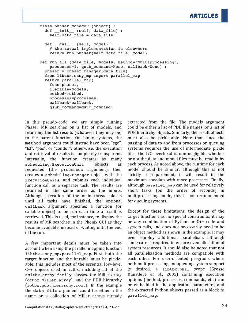
class phaser_manager (object) : def __init__ (self, data_file) : self.data_file = data_file def __call__ (self, model) : # the actual implementation is elsewhere return run_phaser(self.data_file, model) def run_all (data_file, models, method=”multiprocessing”, processes=1, qsub_command=None, callback=None) : phaser = phaser_manager(data_file) from libtbx.easy_mp import parallel_map return parallel_map( func=phaser, iterable=models, method=method, processes=processes, callback=callback, qsub_command=qsub_command)

5

In this pseudo-‐code, we are simply running Phaser MR searches on a list of models, and returning the list results (whatever they may be) to the parent function. On Linux systems, the method argument could instead have been “sge”, “lsf”, “pbs”, or “condor”; otherwise, the execution and retrieval of results is completely transparent. Internally, the function creates as many scheduling.ExecutionUnit objects as requested (the processes argument), then creates a scheduling.Manager object with the ExecutionUnits, and submits each individual function call as a separate task. The results are returned in the same order as the inputs. Although execution of the main thread blocks until all tasks have finished, the optional callback argument specifies a function (or callable object) to be run each time a result is retrieved. This is used, for instance, to display the results of MR searches in the Phenix GUI as they become available, instead of waiting until the end of the run. A few important details must be taken into account when using the parallel mapping function libtbx.easy_mp.parallel_map. First, both the target function and the iterable must be pickle-‐able: this includes most of the essential low-‐level C++ objects used in cctbx, including all of the scitbx.array_family classes, the Miller array (cctbx.miller.array), and the PDB hierarchy (iotbx.pdb.hierarchy.root). In the example the data_file argument could be either a file name or a collection of Miller arrays already

6

extracted from the file. The models argument could be either a list of PDB file names, or a list of PDB hierarchy objects. Similarly, the result objects must also be pickle-‐able. Note that since the passing of data to and from processes on queuing systems requires the use of intermediate pickle files, the I/O overhead is non-‐negligible whether or not the data and model files must be read in by each process. As noted above, the runtime for each model should be similar; although this is not strictly a requirement, it will result in the maximum speedup with more processes. Finally, although parallel_map can be used for relatively short tasks (on the order of seconds) in multiprocessing mode, this is not recommended for queuing systems. Except for these limitations, the design of the target function has no special constraints; it may be any combination of Python or C++ code and system calls, and does not necessarily need to be an object method as shown in the example. It may even employ additional parallelism, although some care is required to ensure even allocation of system resources. It should also be noted that not all parallelization methods are compatible with each other. For user-‐oriented programs where both multiprocessing and queuing system support is desired, a libtbx.phil scope (Grosse Kunstleve et al., 2005) containing execution options (method, processes, commands, etc.) can be embedded in the application parameters, and the extracted Python objects passed as a block to parallel_map.


ARTICLES

7

Extending multiprocessing.Pool for greater flexibility The parallel_map function is optimal for new applications where the data to be passed between the parent and the child processes are pickle-‐able. (It is also the only method fully supported on Windows, which has built-‐in limitations that make process-‐level Python parallelism more difficult.)

8

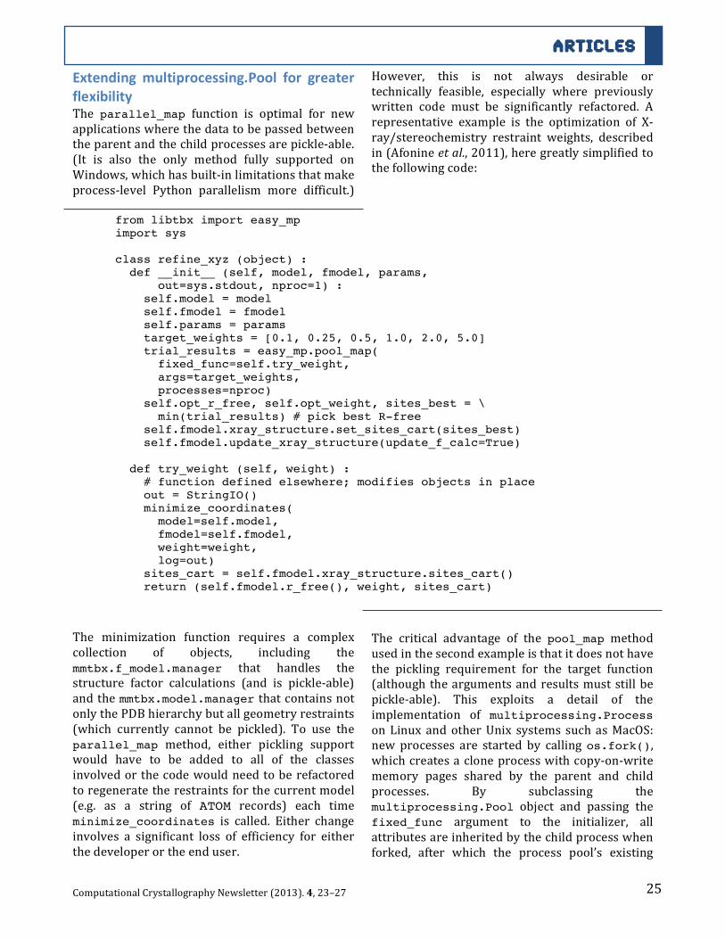
However, this is not always desirable or technically feasible, especially where previously written code must be significantly refactored. A representative example is the optimization of X-‐ray/stereochemistry restraint weights, described in (Afonine et al., 2011), here greatly simplified to the following code:

9

from libtbx import easy_mp import sys class refine_xyz (object) : def __init__ (self, model, fmodel, params, out=sys.stdout, nproc=1) : self.model = model self.fmodel = fmodel self.params = params target_weights = [0.1, 0.25, 0.5, 1.0, 2.0, 5.0] trial_results = easy_mp.pool_map( fixed_func=self.try_weight, args=target_weights, processes=nproc) self.opt_r_free, self.opt_weight, sites_best = \ min(trial_results) # pick best R-free self.fmodel.xray_structure.set_sites_cart(sites_best) self.fmodel.update_xray_structure(update_f_calc=True) def try_weight (self, weight) : # function defined elsewhere; modifies objects in place out = StringIO() minimize_coordinates( model=self.model, fmodel=self.fmodel, weight=weight, log=out) sites_cart = self.fmodel.xray_structure.sites_cart() return (self.fmodel.r_free(), weight, sites_cart)

10

The minimization function requires a complex collection of objects, including the mmtbx.f_model.manager that handles the structure factor calculations (and is pickle-‐able) and the mmtbx.model.manager that contains not only the PDB hierarchy but all geometry restraints (which currently cannot be pickled). To use the parallel_map method, either pickling support would have to be added to all of the classes involved or the code would need to be refactored to regenerate the restraints for the current model (e.g. as a string of ATOM records) each time minimize_coordinates is called. Either change involves a significant loss of efficiency for either the developer or the end user.

11

The critical advantage of the pool_map method used in the second example is that it does not have the pickling requirement for the target function (although the arguments and results must still be pickle-‐able). This exploits a detail of the implementation of multiprocessing.Process on Linux and other Unix systems such as MacOS: new processes are started by calling os.fork(), which creates a clone process with copy-‐on-‐write memory pages shared by the parent and child processes. By subclassing the multiprocessing.Pool object and passing the fixed_func argument to the initializer, all attributes are inherited by the child process when forked, after which the process pool’s existing


ARTICLES

12

map() method is called. In many practical situations the bulk of the memory pages are never modified by the child processes, and therefore never duplicated. Therefore fork’s copy-‐on-‐write approach not only avoids the pickling overhead for the target function, but also makes it possible to have many child processes even if the parent process already consumes a large fraction of the available memory. Using this method, any existing embarrassingly parallel for loop can be parallelized with the addition of a few lines of code. This is used in several places in phenix.refine and phenix.den_refine, where near-‐linear speedups are achieved for the parallelized loops. The copy-‐on-‐write memory management of the Unix fork() system call keeps the memory overhead to a minimum, and since all other objects are shared in memory, no file I/O is required. The overhead for forking a process is minimal, and if the function arguments (and return values) can be kept small and simple, pickling these will not have a significant impact on runtime. For these reasons, pool_map is also suitable for cases where the individual tasks have runtimes on the order of seconds (e.g. for the validation of ensemble models).

Practical considerations Because libtbx.easy_mp is intended to make parallelization of existing code as easy and non-‐invasive as possible, neither of the methods described here place many restrictions on the implementation of the mapped function. However, following several general guidelines should make the transition easier: • Keep file I/O to a minimum -‐ in particular, avoid any writes to paths or filehandles that may be in use by other processes. Use local “scratch” disks whenever possible if running on a queuing system.

• It is also helpful to keep printed log output to a minimum; any important information that the user needs to see should be saved for display until the result is retrieved in the main process.

• Avoid uncaught exceptions, except where programmer error is likely to be at fault. Errors such as an inappropriate input or a failed calculation should be included in the return value and handled in the main process.

• If the runtime of the target function on each of

13

the arguments is expected to vary and can be guessed or approximated, the arguments that are expected to take the longest should be first in the list.

• For maximum convenience and compatibility, both methods will simply execute a serial for loop over all arguments if number of processes equals 1 or the parallelization method is not supported (such as easy_mp under Windows). This means that no special application-‐level code is required to decide whether or not to use parallelism.

An additional limitation is that unlike the ParallelForIterator described previously (Bunkóczi & Echols, 2013), the parallel map() implementations do not have the option of exiting early if an acceptable result is found. Therefore they are only suitable for tasks where all results need to be collected and analyzed at once. Finally, we emphasize that these libraries are designed for end-‐user applications such as Phenix that must be as portable as possible. They target the computing resources available to the typical crystallographer, i.e. multi-‐core personal computers and workstations ranging from 2 to 64 CPU cores, up to lab-‐ or department-‐scale shared clusters, where the maximum available resources are expected to be, at most, several hundred processor cores. Deployment of the application is intended to require no additional setup or dedicated resources beyond the optional availability of one of the supported queuing systems. It therefore makes several compromises that limit the scalability, in particular the use of the file system for execution on a cluster, and it is not fault-‐tolerant with regards to outright crashes or hardware failures. For applications intended to run on a specific system, or where scalability, stability, and efficiency across thousands of processors are essential, a more specialized (but less portable) platform or API such as MPI or MapReduce1 (Dean & Ghemawat, 2008) should provide significantly better performance.

Availability and platform support Any CCTBX version released after January 2013 has the described functions (this is also included

1 A popular open-‐source implementation, Apache Hadoop (http://hadoop.apache.org), includes Python support, and there does not appear to be any obstacle to using Hadoop as an additional backend in the framework we describe.


ARTICLES

14

in Phenix build 1282 or newer). Support for queuing systems is effectively limited to Linux; the pool_map function is limited to Linux and MacOS

15

(it may still be used on Windows, but will run serially). Additional examples of usage are available by request from the authors.

16

References Adams, P. D., Afonine, P. V., Bunkoczi, G., Chen, V. B., Davis, I. W., Echols, N., Headd, J. J., Hung, L. W.,

Kapral, G. J., Grosse-‐Kunstleve, R. W., McCoy, A. J., Moriarty, N. W., Oeffner, R., Read, R. J., Richardson, D. C., Richardson, J. S., Terwilliger, T. C. & Zwart, P. H. (2010). Acta Crystallogr D 66, 213-‐221.

Afonine, P. V., Echols, N., Grosse Kunstleve, R. W., Moriarty, N. W. & Adams, P. D. (2011). Computational Crystallography Newsletter 2, 99-‐103.

Afonine, P. V., Grosse-‐Kunstleve, R. W., Echols, N., Headd, J. J., Moriarty, N. W., Mustyakimov, M. W., Terwilliger, T. C., Urzhumtsev, A., Zwart, P. H. & Adams, P. D. (2012). Acta Crystallogr D 68, in press.

Bunkóczi, G. & Echols, N. (2012). Computational Crystallography Newsletter 3, 37-‐42. Bunkóczi, G. & Echols, N. (2013). Computational Crystallography Newsletter 4, (in press). Dean, J. & Ghemawat, S. (2008). Communications of the ACM 51, 107-‐113. DiMaio, F., Terwilliger, T. C., Read, R. J., Wlodawer, A., Oberdorfer, G., Wagner, U., Valkov, E., Alon, A.,

Fass, D., Axelrod, H. L., Das, D., Vorobiev, S. M., Iwai, H., Pokkuluri, P. R. & Baker, D. (2011). Nature 473, 540-‐543.

Grosse Kunstleve, R. W., Afonine, P. V., Sauter, N. K. & Adams, P. D. (2005). Newsletter of the IUCr Commission on Crystallographic Computing 5, 69-‐91.

Keegan, R. M. & Winn, M. D. (2008). Acta Crystallogr D Biol Crystallogr 64, 119-‐124. O'Donovan, D. J., Stokes-‐Rees, I., Nam, Y., Blacklow, S. C., Schroder, G. F., Brunger, A. T. & Sliz, P. (2012).

Acta Crystallogr D Biol Crystallogr 68, 261-‐267. Panjikar, S., Parthasarathy, V., Lamzin, V. S., Weiss, M. S. & Tucker, P. A. (2005). Acta Crystallogr D Biol

Crystallogr 61, 449-‐457. Rodriguez, D., Sammito, M., Meindl, K., de Ilarduya, I. M., Potratz, M., Sheldrick, G. M. & Uson, I. (2012).

Acta Crystallogr D Biol Crystallogr 68, 336-‐343. Rodriguez, D. D., Grosse, C., Himmel, S., Gonzalez, C., de Ilarduya, I. M., Becker, S., Sheldrick, G. M. & Uson,

I. (2009). Nat Methods 6, 651-‐653. Schmidberger, J. W., Bate, M. A., Reboul, C. F., Androulakis, S. G., Phan, J. M., Whisstock, J. C., Goscinski, W.

J., Abramson, D. & Buckle, A. M. (2010). Plos One 5, e10049. Schroder, G. F., Levitt, M. & Brunger, A. T. (2010). Nature 464, 1218-‐U1146. Stokes-‐Rees, I. & Sliz, P. (2010). Proc Natl Acad Sci U S A 107, 21476-‐21481. Terwilliger, T. C., Grosse-‐Kunstleve, R. W., Afonine, P. V., Adams, P. D., Moriarty, N. W., Zwart, P., Read, R.

J., Turk, D. & Hung, L. W. (2007). Acta Crystallogr D 63, 597-‐610. Terwilliger, T. C., Grosse-‐Kunstleve, R. W., Afonine, P. V., Moriarty, N. W., Adams, P. D., Read, R. J., Zwart,

P. H. & Hung, L. W. (2008). Acta Crystallogr D 64, 515-‐524. Terwilliger, T. C., Grosse-‐Kunstleve, R. W., Afonine, P. V., Moriarty, N. W., Zwart, P. H., Hung, L. W., Read,

R. J. & Adams, P. D. (2008). Acta Crystallogr D 64, 61-‐69. Terwilliger, T. C., Klei, H., Adams, P. D., Moriarty, N. W. & Cohn, J. D. (2006). Acta Crystallogr D Biol

Crystallogr 62, 915-‐922. van den Bedem, H., Dhanik, A., Latombe, J. C. & Deacon, A. M. (2009). Acta Crystallogr D Biol Crystallogr

65, 1107-‐1117. van den Bedem, H., Wolf, G., Xu, Q. & Deacon, A. M. (2011). Acta Crystallogr D Biol Crystallogr 67, 368-‐

375.

Documents

CCN 2013 01 v06 - Phenixphenix-online.org/newsletter/CCN_2013_01.pdf · 2013-04-09 · Computational!Crystallography!Newsletter!(2013).!Volume!4,!Part!1.! 3! 5 feature! that! may!