cchdo.ucsd.edu · Web viewThe ship's position was measured by navigation system made by FURUNO ELECTRIC CO., LTD. JAPAN. The system has two 3-channels GPS receivers (GP-80, GP-150)

B. Underway measurements1. Navigation and Bathymetry

(1) Personnel

Takahiro SEGAWA (GEMD/JMA)

Tetsuya NAKAMURA (GEMD/JMA)

Keizo SHUTTA (GEMD/JMA)

Yoshikazu HIGASHI (GEMD/JMA)

Tomoyuki KITAMURA (GEMD/JMA)

Yasuaki BUNGI (GEMD/JMA)

(2) Navigation

(2.1) Overview of the equipment

The ship's position was measured by navigation system made by FURUNO ELECTRIC CO.,

LTD. JAPAN. The system has two 3-channels GPS receivers (GP-80, GP-150). GPS antennas

was installed at Compass deck. We switched the receivers to choose better receiving state if

the number of GPS satellites decreased or HDOP increased. GPS data, gyro heading and log

speed were integrated and delivered to two workstations. One workstation works as primary

NTP (Network Time Protocol) server and the other works secondary server.

The navigation data were obtained approximately every one second and one minute data were

extract from one second data. These one minute data were recorded as "LOG data".

(2.2) Data Period

05:00, 06 Jul. 2010 to 00:00, 1 Sep. 2010(UTC)

(3) Bathymetry

(3.1) Overview of the equipment

R/V Ryofu Maru equipped a single beam echo sounder, Kongsberg EA 600 (SIMRAD

Fisheries Research, Norway). The main objective of the survey is collecting continuous

bathymetry data along ship's track. At first we set up system choosing 1500 m/s for sound

speed. During the cruise, we used averaged sound velocity data obtained from the nearest

CTD cast to get accurate depth data. Data interval was about 8 seconds at 6000m.

(3.2) System Configuration and Performance

System: Kongsberg EA 600

Frequency: 12kHz

Transmit power: 2kW

Transmit pulse interval: Within 20seconds

Depth range: 5 to 15,000m

Depth resolution: 1cm

Depth accuracy: Within 20cm

(3.3) Data Period

The collecting bathymetry data was carried out during the cruise except for port of Palau and

Saipan.

05:00, 06 Jul. 2010 to 00:00, 1 Sep. 2010(UTC)

(3.4) Data Processing

The bathymetry data are obtained using a mean sound velocity calculated from the data of

nearest CTD cast. The formula of the sound velocity calculated in SEASAVE, CTD data

acquisition software, is Chen and Millero (1977). The system combines bathymetry data with

navigation data, so the data file consists of date, time, location, depth and flag of bathymetry

data.

If the erroneous data were obtained, the bathymetry data flag was set to '9' and the data was

set to '0' automatically.

Reference

Chen, C.-T. and F. J. Millero (1977): Speed of sound in seawater at high pressures. J. Acoust.

Soc. Am. 62(5), 1129-1135.

2. Maritime Meteorological Observations

(1) Personnel







(2) Data Period

09:00, 6 Jul. 2010 to 23:00, 31 Aug. 2010(UTC)

(3) Methods

The maritime meteorological observation system on R/V Ryofu Maru is Ryofu Maru maritime

meteorological measurement station (RMET). Instruments of RMET are listed in Table B.2.1.

All RMET data were collected and processed by KOAC-7800 weather data processor made

by Koshin Denki Kogyo CO., Ltd. Japan.

Figure B.2.1 and B.2.2 show maritime meteorological observation data.

Table B.2.1. Instruments and locations of RMET.

Sensor Parameter Manufacture Location

(Type) (Height from maximum

load line)

Thermometer Air Temperature Koshin Denki Kogyo

(Electric type)

Compass deck

(13.3m)

Hygrometer Relative humidity Koshin Denki Kogyo

(Electrostatic type)

Compass deck

(13.3 m)

Thermometer Sea Temperature Koshin Denki Kogyo Engine Room

(Electric type) (–4.7 m)

Aerovane Wind Speed Koshin Denki Kogyo Mast top

Wind Direction (Propellar type) (19.8 m)

Wave gauge Wave Height Tsurumi-Seiki Ship front

Wave period (Micro wave type) (6.5 m)

Barometer Pressure Koshin Denki Kogyo Observation room

(Electrostatic type) (2.8 m)

Note that there are two set of thermometer and hygrometer at starboard and port sides.

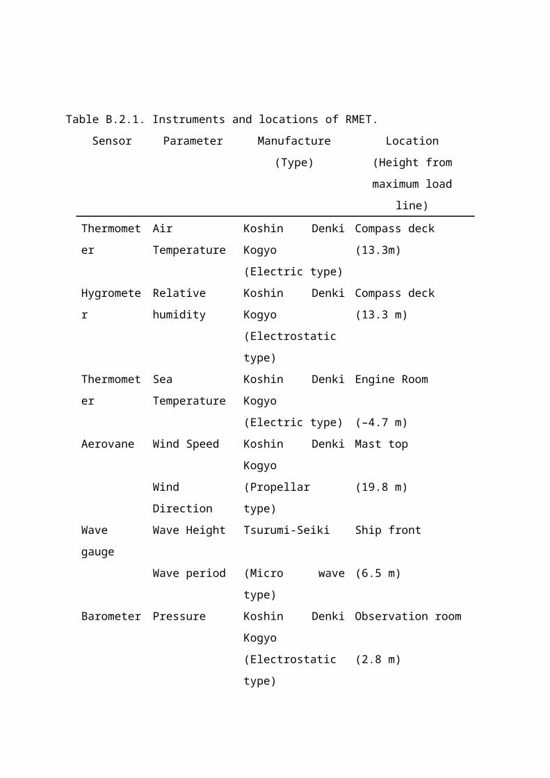
Figure B.2.1. Time series of (a) air and sea surface temperature, (b) relative humidity, (c)

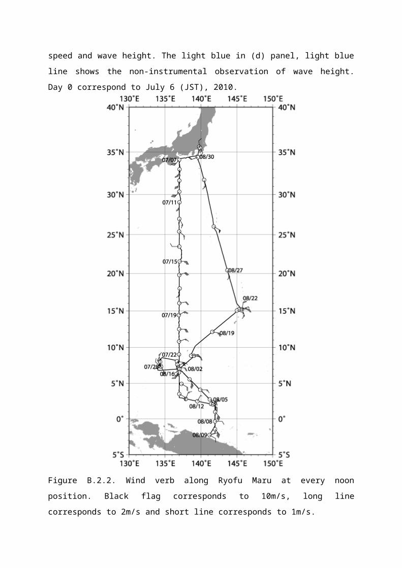
pressure, (d) wind speed and wave height. The light blue in (d) panel, light blue line shows

the non-instrumental observation of wave height. Day 0 correspond to July 6 (JST), 2010.

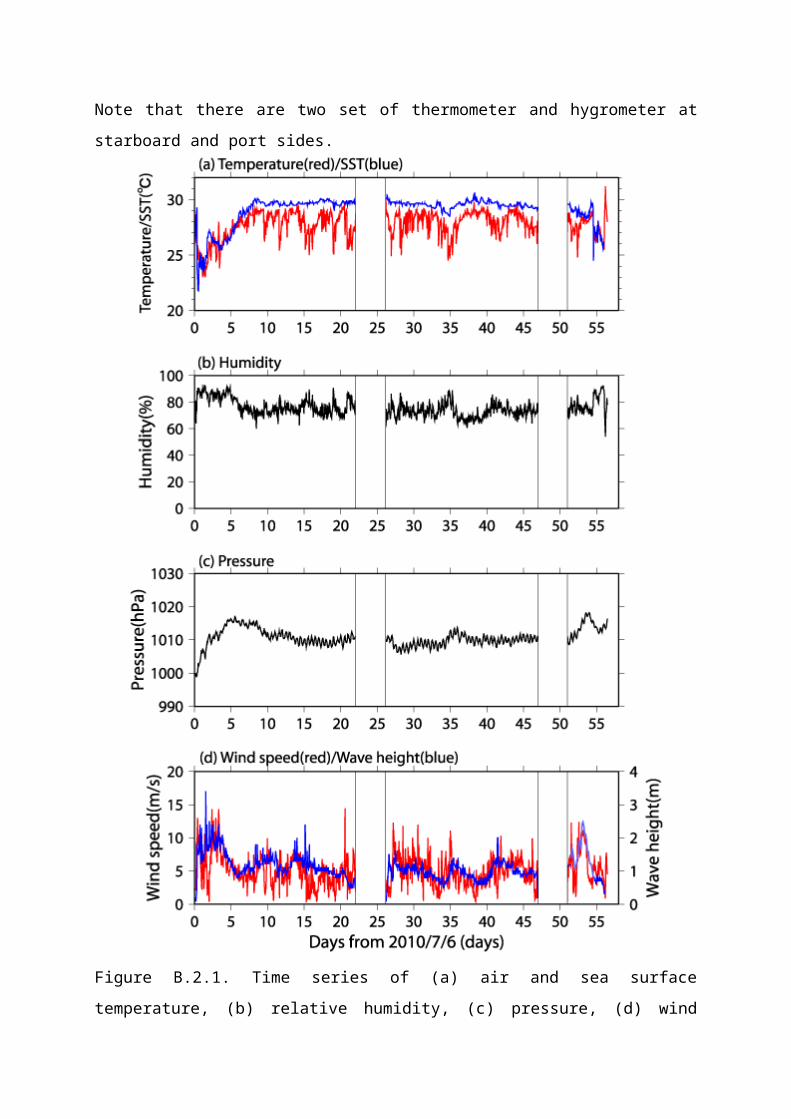
Figure B.2.2. Wind verb along Ryofu Maru at every noon position. Black flag corresponds to

10m/s, long line corresponds to 2m/s and short line corresponds to 1m/s.

(4) Data processing and Data format

All raw data were recorded every 6-seconds. 1-minute and 10-minute values are averaged

from 6-seconds values. 10-minute value of every three hours is available at JMA web site

(http://www.data.kishou.go.jp/kaiyou/db/vessel_obs/data-report/html/ship/cruisedata_e.php?

id=RF1005).

Since the thermometers and hygrometers are equipped on both starboard/port sides on the

Compass deck, we used air temperature/relative humidity data taken at upwind side. Dew

point temperature was calculated from relative humidity and air temperature data.

No adjustment to sea level values is applied except for pressure data. During the cruise, fixed

value +0.5hPa is used for sea level correction. Data are stored in ASCII format and

representative parameters are as follows. Time in UTC, longitude (E), latitude (N), ship speed

(knot), ship direction (degrees), sea surface pressure (hPa), air temperature (degrees Celsius),

dew point temperature (degrees Celsius), relative humidity (%), sea surface temperature

(degrees Celsius), wind direction (degree) and wind speed (m/sec).

Wave height and period are observed twice an hour. The sampling duration is 20 minutes and

each sampling starts at 5 minutes and 35 minutes after the hour. In addition to those data,

ship’s position and observation time are recorded in ASCII format.

(5) Data quality

To ensure the data quality, each sensor was checked as follows.

Temperature/Relative humidity sensor:

Temperature and relative humidity (T/RH) sensors were checked by manufacturer and, they

were also checked by using calibrated Asman psychrometer before the cruise and arrival at

the port. The discrepancy between T/RH sensors and Asman psychrometer were within ±0.4

degrees Celsius and ±4 % respectively at both sides.

Thermometer (Sea Temperature):

Sea temperature sensor was calibrated once per year by the manufacturer. Certificated

accuracy of sea temperature sensor is better than ±0.4 degrees Celsius. The values are also

compared with bucket samples after the departure.

Pressure sensor:

Using calibrated portable barometer (Vaisala 765-16B, certificated accuracy is better than ±

0.1 hPa), pressure sensor was checked before the cruise. Mean difference of RMET pressure

sensor and portable sensor is less than 0.7 hPa.

Aerovane:

Aerovane was checked once per year by the manufacturer and, once per five years by the

Meteorological Instrument Center, JMA.

(6) Ship’s weather observation

Non-instrumental observations such as weather, cloud, visibility, wave direction and wave

height were made by the ship crews every three hours. We sent those data together with

RMET data to the Global Collecting Centre for Marine Climatological Data in IMMT

(International Maritime Meteorological Tape) -III format. The RMET data is available at JMA

web site.

(http://www.data.kishou.go.jp/kaiyou/db/vessel_obs/data-report/html/ship/cruisedata_e.php?

id=RF1005).

3. CO2　and Thermo-Salinograph

(1) Personnel

　　　Shinji Masuda (JMA)

　　　Kazutaka Enyo (JMA)

Kazuki Ishimaru (JMA)

Etsuro Ono (JMA)

Naohiro Kosugi (MRI)

(2) Instrument and sampling

Partial pressure of CO2 (pCO2) in atmosphere and in surface seawater were measured with the

CO2 measuring system manufactured by Nippon ANS, Inc. based on the method described by

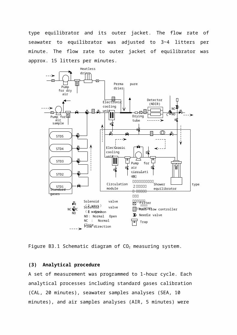
Inoue et al. (1999) and Dickson et al. (2007). The system comprises of a non-dispersive

infrared gas analyzer (NDIR) (LI-COR LI7000), an air-circulation module and a showerhead-

type equilibrator (Figure B3.1). The thermo-salinograph (TSG) (Sea–Bird Electronics, Inc.

SBE 38 and SBE 45) was used for measuring temperature and salinity of surface seawater

sample; both temperature and salinity were used for calculation of CO2 concentration of

seawater. The measurement system was automatically controlled by using a personal

computer equipped with A/D conversion board.

Air sample was taken from the air intake at the bow of the ship, about 8-meters height above

the water level. The air sample was transferred to the measurement apparatus through a 3/8-

inch diameter fluorinated ethylene-perfluoroalkoxyethylene copolymer (Teflon® PFA) tube.

Surface seawater was pumped from the water intake at about 4-meters depth below the water

level and was supplied to shower-type equilibrator and its outer jacket. The flow rate of

seawater to equilibrator was adjusted to 3~4 litters per minute. The flow rate to outer jacket of

equilibrator was approx. 15 litters per minutes.

Figure B3.1 Schematic diagram of CO2 measuring system.

(3) Analytical procedure

A set of measurement was programmed to 1-hour cycle. Each analytical processes including

standard gases calibration (CAL, 20 minutes), seawater samples analyses (SEA, 10 minutes),

and air samples analyses (AIR, 5 minutes) were combined as CAL-SEA-AIR-SEA-AIR-SEA.

Air samples and standard gas analyses were made using following procedure;

1) The air sample was dried using electronic cooling unit (dew point of 2ºC) followed by

passing through drying tube (magnesium perchlorate desiccant) prior to transfer into the

NDIR.

2) NDIR cell was flushed with the air sample for 250 seconds. The flow rate was regulated

Detector (NDIR)

Heatless drier

Drying tube

Perma pure drierPump for

dry air

Standard gases

STD1

Pump for air sample

Circulation moduleShower type equilibrator

Electronic cooling unit

ポンプ

付属バルブ刻印アウトレットキャップ２次圧ゲージ１次圧ゲージ調圧弁保護キャップ

循環空気用ポンプ (cH16)

Pump for air circulation

STD5

STD4

STD3

STD2

Electronic cooling unit

Filter

Mass flow controller

Needle valve

Trap

CNO

NC

Solenoid valve （ 2 ways）Solenoid valve （ 3 ways）

Flow direction

C： Common NO： Normal　 OpenNC： Normal　 Close

NO

NC

C

to 500 cm3/min using mass flow controller.

3) The NDIR inner pressure was let loose by atmospheric pressure for 15 seconds.

4) The outputs of NDIR, temperature of NDIR cell and air pressure at NDIR were recorded

for 30 seconds with 1 second interval.

Seawater samples analyses were made using following procedure;

5) The air inside the equilibrator was circulated through the air-circulation module that

includes equilibrator for 550 seconds to reach equilibrium with respect to CO2 exchange

between seawater and the air in the circulation module.

6) The air in the circulation module was dried, transferred to NDIR and analysed in the

same way described above 2) – 4).

(4) Calibration

The NDIR analyzer was calibrated at interval of 1 hour using a set of CO2 standard gas

cylinders. The concentrations of CO2 standard gases are listed in Table B3.1, which were pre-

calibrated and post-calibrated with the WMO mole-fraction scale.

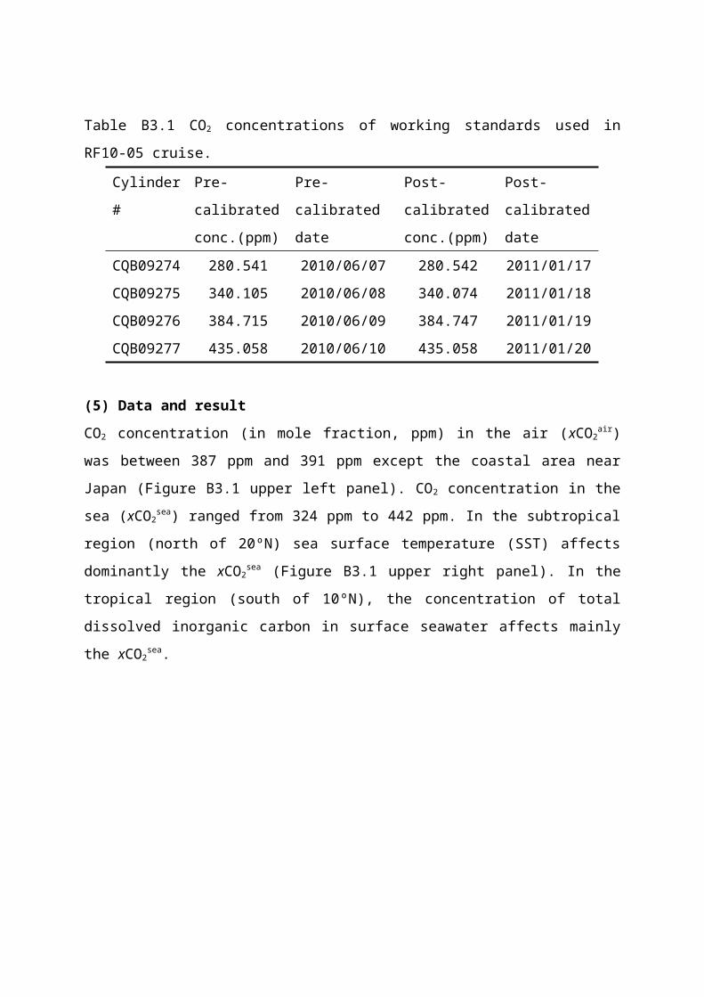
Table B3.1 CO2 concentrations of working standards used in RF10-05 cruise.

Cylinder # Pre-calibrated

conc.(ppm)

Pre-calibrated

date

Post-calibrated

conc.(ppm)

Post-calibrated

date

CQB09274 280.541 2010/06/07 280.542 2011/01/17

CQB09275 340.105 2010/06/08 340.074 2011/01/18

CQB09276 384.715 2010/06/09 384.747 2011/01/19

CQB09277 435.058 2010/06/10 435.058 2011/01/20

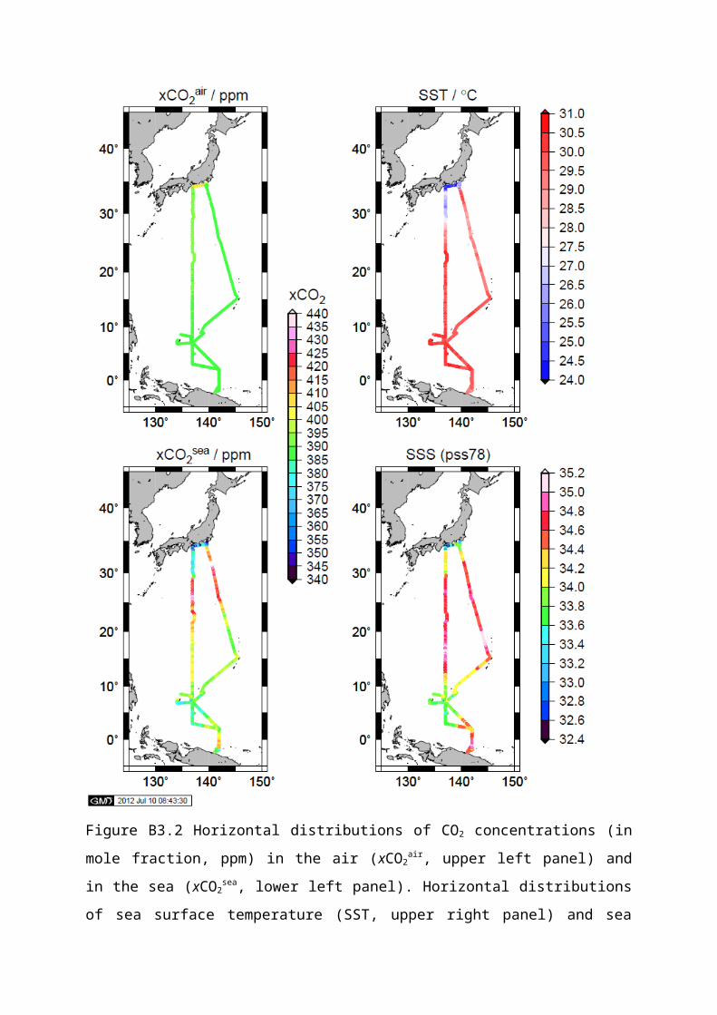
(5) Data and result

CO2 concentration (in mole fraction, ppm) in the air (xCO2air) was between 387 ppm and 391

ppm except the coastal area near Japan (Figure B3.1 upper left panel). CO2 concentration in

the sea (xCO2sea) ranged from 324 ppm to 442 ppm. In the subtropical region (north of 20ºN)

sea surface temperature (SST) affects dominantly the xCO2sea (Figure B3.1 upper right panel).

In the tropical region (south of 10ºN), the concentration of total dissolved inorganic carbon in

surface seawater affects mainly the xCO2sea.

Figure B3.2 Horizontal distributions of CO2 concentrations (in mole fraction, ppm) in the air

(xCO2air, upper left panel) and in the sea (xCO2

sea, lower left panel). Horizontal distributions of

sea surface temperature (SST, upper right panel) and sea surface salinity (SSS, lower right

panel).

References

Dickson, A.G., Sabine, C.L. and Christian, J.R. (Eds.) (2007): Guide to best practices for

ocean CO2 measurements. PICES Special Publication 3, 191 pp.

Inoue, Y. H., M. Ishii, H. Matsueda, S. Saito T. Midorikawa and K. Nemoto (1999): MRI

measurements of　 partial　 pressure　 of　CO2　 in　 surface　waters　 of　 the

Pacific　during　1968　 to　1970:　 re-evaluation　and　comparison of data with

those of the 1980s and 1990s, Tellus, 51B, 830-848.

4. Chlorophyll-a

(1) Personnel

　　　Yusuke TAKATANI (GEMD/JMA)

　　　Shinichiro UMEDA (GEMD/JMA)

(2) Method

The Continuous Sea Surface Water Monitoring System of fluorescence (Nippon Kaiyo Co.

Ltd.) automatically had been continuously measured seawater which is pumped from a depth

of about 4.5 m below the maximum load line to the laboratory. The flow rate of the surface

seawater was controlled by several valves and adjusted to about 0.6 L/min. The sensor in this

system is a fluorometer (10-AU, S/N:7063) manufactured by Turner Designs. The system

measured every one minute.

(3) Measurement

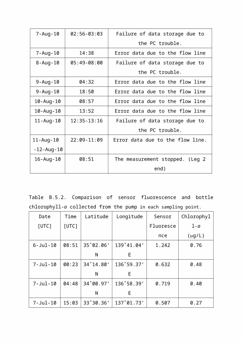
Periods of measurement and problems are listed in Table B.5.1.

(4) Calibration

In order to calibrate the fluorescence sensor, we collected 200 ml of surface seawater from

outlet of water line of the system for measuring chlorophyll-a. The seawater samples were

collected at nominally 60 N. miles intervals. The seawater sample was gently filtrated by low

vacuum pressure through Whatman GF/F filter (diameter 25mm). The filter was immediately

transferred into 9 ml of N, N-dimethylformamide (DMF) and then stored at –30ºC to extract

chlorophyll-a for more than 24 hours. Concentrations of chlorophyll-a were measured by a

fluorometer (10-AU, S/N: 6718, TURNER DESIGNS) that was previously calibrated against

a pure chlorophyll-a (Lot.:BCBB4166, Sigma chemical Co.) by the method described in

UNESCO (1994). In order to calibrate the fluorometer, fluorometric measurement of

chlorophyll-a was performed by the method of Holm-Hansen et al. (1965) and Holm-Hansen

and Riemann (1978). The results of the measurements are shown in Table B.5.2. The

fluorescence sensor may be contaminated while measuring. Therefore,　we calibrated the

fluorescence value of the sensor to 0 (deionized water) and 10 (0.1 ppm Rhodamine solution)

at the start of a leg, and measured a solution of the same concentration at the end of a leg. The

results are shown in Table B.5.3.

The data is calculated by the following procedure;

- The fluorescence value of the sensor is calibrated by deionized water and a Rhodamine

solution at the starting and the ending.

- The ratio between a calibrated fluorescence value and a chlorophyll-a concentration of a

seawater sample is interpolated by distance.

- The chlorophyll-a concentration is calculated by multiplying a calibrated fluorescence value

by an interpolated ratio.

(5) Data and Result

Quality controlled data, those file name is “20120202_p09_in-vivo.txt”, is distributed by JMA

format. The record structure of JMA format is shown below.

Column1: observed date [UTC]

Column2: observed time [UTC]

Column3: observed latitude

Column4: observed longitude

Column5: fluorescence value

Column6: fluorescence value calibrated by deionized water and a Rhodamine solution

Column7: ratio between a calibrated fluorescence value and a chlorophyll-a concentration

of a seawater sample interpolated by distance

Column8: calculated chlorophyll-a concentration (g/L)

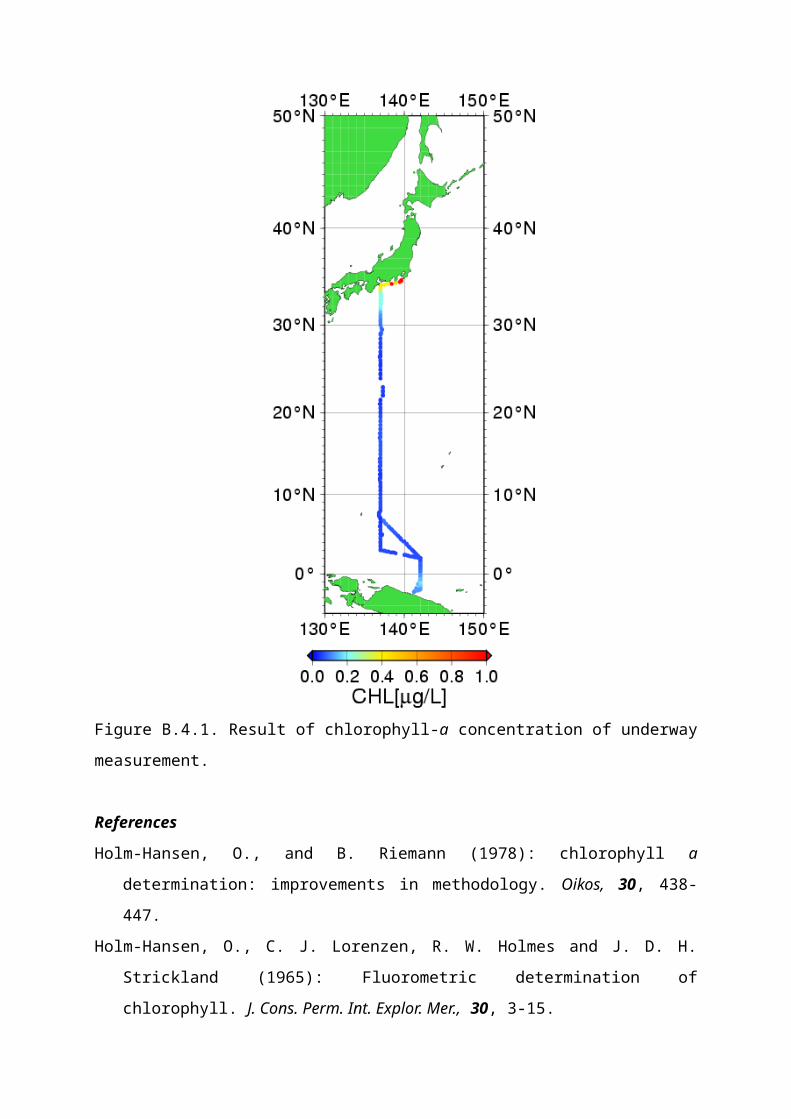
Result of chlorophyll-a concentration of underway measurement in shown in Figure B.4.1.

Chlorophyll-a data on Figure B.4.1 is averaged over 2-hours.

Figure B.4.1. Result of chlorophyll-a concentration of underway measurement.

References

Holm-Hansen, O., and B. Riemann (1978): chlorophyll a determination: improvements in

methodology. Oikos, 30, 438-447.

Holm-Hansen, O., C. J. Lorenzen, R. W. Holmes and J. D. H. Strickland (1965): Fluorometric

determination of chlorophyll. J. Cons. Perm. Int. Explor. Mer., 30, 3-15.

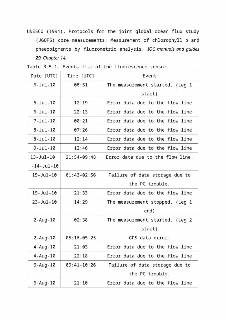
UNESCO (1994), Protocols for the joint global ocean flux study (JGOFS) core

measurements: Measurement of chlorophyll a and phaeopigments by fluorometric

analysis, IOC manuals and guides 29, Chapter 14.

Table B.5.1. Events list of the fluorescence sensor.

Date [UTC] Time [UTC] Event

6-Jul-10 08:51 The measurement started. (Leg 1 start)

6-Jul-10 12:19 Error data due to the flow line






13-Jul-10

-14-Jul-10

21:54-09:48 Error data due to the flow line.

15-Jul-10 01:43-02:56 Failure of data storage due to the PC trouble.


23-Jul-10 14:29 The measurement stopped. (Leg 1 end)

2-Aug-10 02:38 The measurement started. (Leg 2 start)

2-Aug-10 05:16-05:25 GPS data error.

4-Aug-10 21:03 Error data due to the flow line


6-Aug-10 09:41-10:26 Failure of data storage due to the PC trouble.










11-Aug-10 22:09-11:09 Error data due to the flow line.

-12-Aug-10

16-Aug-10 08:51 The measurement stopped. (Leg 2 end)

Table B.5.2. Comparison of sensor fluorescence and bottle chlorophyll-a collected from the

pump in each sampling point.

Date

[UTC]

Time

[UTC]

Latitude Longitude Sensor

Fluorescence

Chlorophyll-a

(g/L)

6-Jul-10 08:51 35˚02.06’N 139˚41.04’E 1.242 0.76

7-Jul-10 00:23 34˚14.80’N 136˚59.37’E 0.632 0.48

7-Jul-10 04:48 34˚00.97’N 136˚58.39’E 0.719 0.40

7-Jul-10 15:03 33˚30.36’N 137˚01.73’E 0.507 0.27

8-Jul-10 04:05 33˚03.12’N 137˚03.42’E 0.240 0.21

8-Jul-10 17:38 32˚21.66’N 137˚04.83’E 0.261 0.18

9-Jul-10 05:14 31˚43.51’N 136˚58.28’E 0.453 0.27

9-Jul-10 17:49 30˚58.89’N 137˚02.15’E 0.157 0.09

10-Jul-10 10:38 30˚00.04’N 137˚02.44’E 0.098 0.08

11-Jul-10 03:01 29˚03.78’N 137˚00.31’E 0.056 0.08

11-Jul-10 16:00 27˚59.81’N 136˚58.89’E 0.050 0.04

12-Jul-10 04:43 27˚00.72’N 136˚59.28’E 0.070 0.04

12-Jul-10 19:01 25˚59.15’N 136˚58.26’E 0.049 0.04

13-Jul-10 08:27 25˚01.70’N 137˚00.67’E 0.038 0.04

13-Jul-10 21:52 24˚01.35’N 136˚59.80’E 0.043 0.05

14-Jul-10 12:37 23˚01.36’N 137˚17.09’E 0.009 0.04

15-Jul-10 00:14 21˚59.46’N 137˚16.84’E -0.004 0.05

15-Jul-10 13:39 21˚00.03’N 136˚55.59’E 0.025 0.03

16-Jul-10 01:15 19˚57.38’N 136˚59.99’E 0.029 0.05

16-Jul-10 13:25 18˚59.38’N 136˚58.47’E 0.086 0.07

17-Jul-10 03:10 18˚00.68’N 137˚02.40’E 0.050 0.07

17-Jul-10 17:16 17˚00.64’N 136˚55.61’E 0.127 0.07

18-Jul-10 06:56 16˚00.56’N 136˚57.81’E 0.129 0.08

18-Jul-10 18:48 14˚58.61’N 136˚58.13’E 0.183 0.07

19-Jul-10 08:19 13˚59.99’N 136˚57.16’E 0.145 0.06

19-Jul-10 21:45 12˚59.91’N 136˚57.25’E 0.193 0.06

20-Jul-10 11:13 12˚00.11’N 136˚56.43’E 0.151 0.03

21-Jul-10 01:28 11˚00.56’N 136˚56.68’E 0.212 0.06

21-Jul-10 14:50 10˚00.13’N 136˚58.09’E 0.242 0.04

22-Jul-10 02:57 9˚00.78’N 136˚57.52’E 0.229 0.06

22-Jul-10 17:19 7˚59.83’N 136˚58.61’E 0.339 0.06

23-Jul-10 14:29 7˚00.36’N 136˚58.13’E 0.510 0.05

2-Aug-10 02:38 7˚01.80’N 136˚59.66’E 0.105 0.10

4-Aug-10 11:23 3˚45.89’N 140˚14.74’E -0.111 0.04

5-Aug-10 00:09 3˚00.95’N 140˚57.80’E -0.104 0.06

5-Aug-10 17:49 1˚59.73’N 141˚58.66’E -0.099 0.05

7-Aug-10 03:43 0˚59.99’N 141˚58.33’E -0.024 0.09

7-Aug-10 12:11 0˚29.74’N 141˚57.93’E -0.060 0.06

7-Aug-10 14:37 0˚14.75’N 141˚59.47’E 0.633 0.13

7-Aug-10 21:35 0˚00.34’N 141˚57.14’E 0.288 0.14

8-Aug-10 14:29 0˚59.78’S 141˚57.93’E 0.147 0.13

9-Aug-10 16:39 2˚00.22’S 141˚57.71’E -0.033 0.14

10-Aug-10 22:56 1˚58.91’N 141˚59.16’E -0.124 0.05

11-Aug-10 09:50 2˚11.62’N 140˚57.94’E -0.101 0.05

11-Aug-10 22:08 2˚24.47’N 139˚58.34’E -0.064 0.06

12-Aug-10 11:12 2˚35.48’N 138˚59.16’E -0.071 0.05

13-Aug-10 01:37 2˚47.76’N 137˚59.88’E -0.068 0.05

13-Aug-10 17:37 2˚59.39’N 136˚59.57’E -0.009 0.07

14-Aug-10 09:46 4˚00.91’N 136˚57.92’E -0.050 0.04

15-Aug-10 00:09 4˚59.68’N 136˚59.26’E -0.014 0.06

15-Aug-10 18:15 5˚58.61’N 136˚56.93’E -0.004 0.05

16-Aug-10 08:51 6˚59.93’N 136˚58.48’E -0.009 0.04

Table B.5.3. Results of the fluorescence value of the sensor at the start and end of each leg(0 :

deionized water, 10 : 0.1ppm Rhodamine solution).

Start End

Date [UTC] 0 10 Date [UTC] 0 10

1 Leg 6-Jul-10 08:30 0 10.000 27-Jul-10 05:00 0 8.296

2 Leg 1-Aug-10 04:30 0 10.000 20-Aug-10 01:32 0 8.438

5. Acoustic Doppler Current Profiler

(1) Personnel







(2) Instruments and Methods

The instrument used was the hull-mounted 38kHz Ocean Surveyor ADCP (Teledyne RD

Instruments, Inc., USA; hereafter TRDI). The transducer of the system was installed in a

dome at 3 m left of center and 13 m aft of the bow at the water line. The firmware version was

23.17 and the data acquisition software was TRDI/VMDAS Version. 1.46. The instrument

was used in water-tracking mode during the operations, and was recording each ping raw data

in 20 m × 60 bin from about 36 m to 1200 m in depth. Sampling interval was variable as short

as possible and typically 6.4 seconds. GPS navigation data and ship’s gyrocompass data were

recorded with the ADCP data. In addition to the raw data, 60 seconds and 300 seconds

averaged data were stored as short time average (STA) and long time average (LTA) data,

respectively. Current field based on the gyrocompass was used to check the operation and the

performance on board.

(3) Performance and quick view of the ADCP data on board

The performance of the ADCP instrument was almost good throughout the cruise, and current

profiles were usually reached about 1000m. We monitored the profiles and currents based on

LTA data in this cruise on board. The ADCP had been installed on the R/V Ryofu Maru just

before the cruise, so the scale factor and misalignment angle (Joyce, 1989) to ADCP firmware

for Leg 1 were set 1.0 and 0.0, respectively. The scale factor and misalignment for Leg 2 and

Leg 3 were set 1.0012 and –1.0627, respectively, based on the calibration constants evaluated

by the Leg 1 data.

(4) Data Processing

LTA data were processed by using CODAS (Common Oceanographic Data Access System)

software, developed at the University of Hawaii

(http://currents.soest.hawaii.edu/docs/doc/index.html). We use a standard CODAS processing

including a PC time correction, a sound-speed correction based on the thermistor temperature

at the transducers, and an amplitude and phase calibration constant applied to the measured

velocities.

Calibration constants to be applied were evaluated for each leg using the water track data. For

Leg 1, the amplitude and phase were 1.0012 and –1.0627, respectively, and for Leg 2 and Leg

3, those were 1.0005 and –0.5528, respectively. Figure B.6.1 shows surface current at the

depth of 36 m during the cruise.

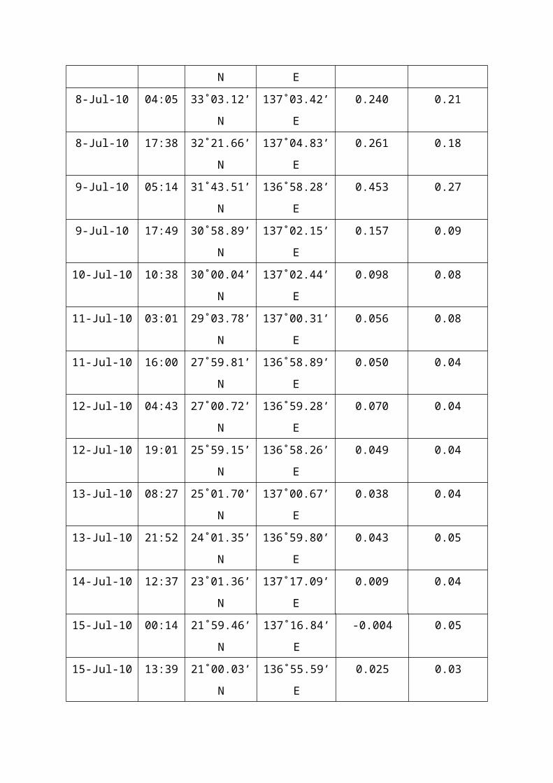
Figure B.6.1. Surface current at the depth of 36 m.

Reference

Joyce, T. M. (1988): On in-situ “calibration” of shipboard ADCPs. J. Atmos. Oceanic

Technol., 6, 169-172.

Documents

cchdo.ucsd.edu · Web viewThe ship's position was measured by navigation system made by FURUNO ELECTRIC CO., LTD. JAPAN. The system has two 3-channels GPS receivers (GP-80, GP-150)