Embed Size (px)
Citation preview
CCACommon Component Architecture
CCA Forum Tutorial Working Grouphttp://www.cca-forum.org/tutorials/
A Look at More Complex Component-Based Applications
Complex Applications CCACommon Component Architecture
2
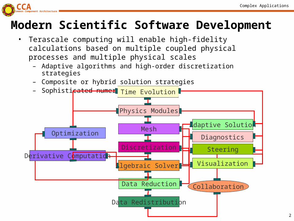
Modern Scientific Software Development• Terascale computing will enable high-fidelity calculations based on
multiple coupled physical processes and multiple physical scales – Adaptive algorithms and high-order discretization strategies– Composite or hybrid solution strategies– Sophisticated numerical tools
Discretization
Algebraic Solvers
Data Redistribution
Mesh
Data Reduction
Physics Modules
Optimization
Derivative Computation
Collaboration
Diagnostics
Steering
Visualization
Adaptive Solution
Time Evolution
Complex Applications CCACommon Component Architecture
3
Overview
• Using components in high performance simulation codes– Examples of increasing complexity– Performance
• Single processor
• Scalability
• Developing components for high performance simulation codes– Strategies for thinking about your own application– Developing interoperable and interchangeable components
Complex Applications CCACommon Component Architecture
4
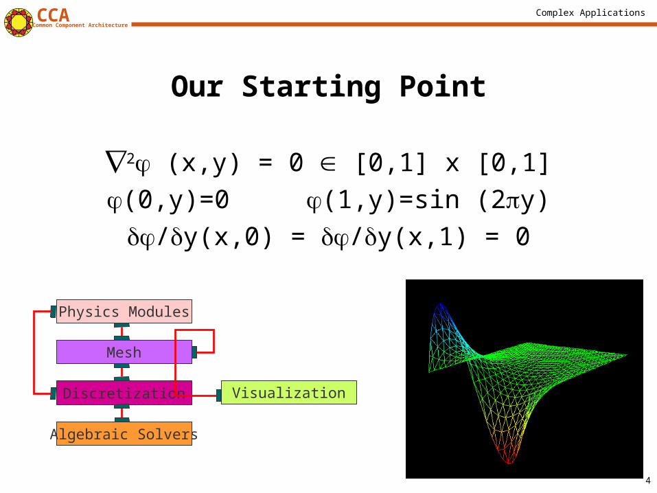
Our Starting Point
2 (x,y) = 0 [0,1] x [0,1]
(0,y)=0 (1,y)=sin (2y)
/y(x,0) = /y(x,1) = 0
Discretization
Algebraic Solvers
Mesh
Physics Modules
Visualization
Complex Applications CCACommon Component Architecture
5
Numerical Solution of Example 1
• Physics: Poisson’s equation• Grid: Unstructured triangular mesh • Discretization: Finite element method• Algebraic Solvers: PETSc (Portable
Extensible Toolkit for Scientific Computation)• Visualization: VTK tool• Original Language: C
Complex Applications CCACommon Component Architecture
6
Creating Components: Step 1
• Separate the application code into well-defined pieces that encapsulate functionalities– Decouple code along numerical functionality
• Mesh, discretization, solver, visualization
• Physics is kept separate
– Determine what questions each component can ask of and answer for other components (this determines the ports)
• Mesh provides geometry and topology (needed by discretization and visualization)
• Mesh allows user defined data to be attached to its entities (needed by physics and discretization)
• Mesh does not provide access to its data structures
– If this is not part of the original code design, this is by far the hardest, most time-consuming aspect of componentization
Complex Applications CCACommon Component Architecture
7
Creating the Components: Step 2
• Writing C++ Components– Create an abstract base class for each port– Create C++ objects that inherit from the abstract base port
class and the CCA component class– Wrap the existing code as a C++ object– Implement the setServices method
• This process was significantly less time consuming (with an expert present) than the decoupling process– Lessons learned
• Definitely look at an existing, working example for the targeted framework
• Experts are very handy people to have around ;-)
Complex Applications CCACommon Component Architecture
8
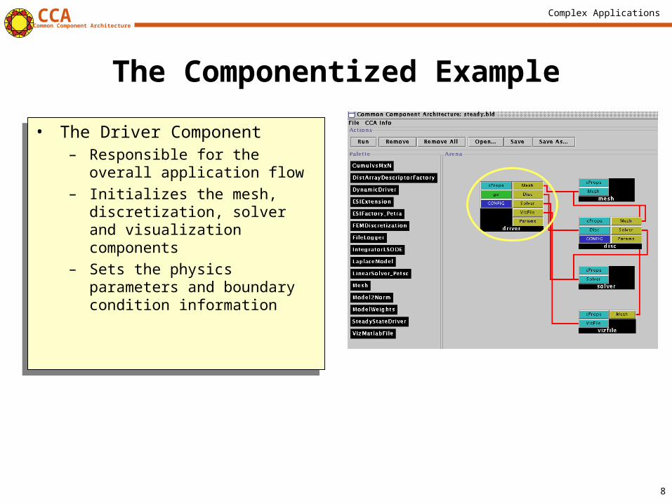
The Componentized Example
• The Driver Component – Responsible for the overall
application flow– Initializes the mesh, discretization,
solver and visualization components
– Sets the physics parameters and boundary condition information
• The Driver Component – Responsible for the overall
application flow– Initializes the mesh, discretization,
solver and visualization components
– Sets the physics parameters and boundary condition information
Complex Applications CCACommon Component Architecture
9
The Componentized Example
• The Driver Component – Responsible for the overall
application flow– Initializes the mesh, discretization,
solver and visualization components
– Sets the physics parameters and boundary condition information
• The Driver Component – Responsible for the overall
application flow– Initializes the mesh, discretization,
solver and visualization components
– Sets the physics parameters and boundary condition information
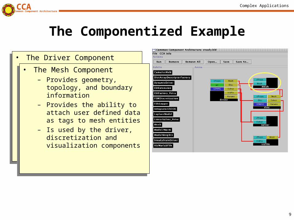
• The Mesh Component– Provides geometry, topology, and
boundary information– Provides the ability to attach user
defined data as tags to mesh entities
– Is used by the driver, discretization and visualization components
• The Mesh Component– Provides geometry, topology, and
boundary information– Provides the ability to attach user
defined data as tags to mesh entities
– Is used by the driver, discretization and visualization components
Complex Applications CCACommon Component Architecture
10
The Componentized Example
• The Driver Component – Responsible for the overall
application flow– Initializes the mesh, discretization,
solver and visualization components
– Sets the physics parameters and boundary condition information
• The Driver Component – Responsible for the overall
application flow– Initializes the mesh, discretization,
solver and visualization components
– Sets the physics parameters and boundary condition information
• The Mesh Component– Provides geometry and topology
information– Provides the ability to attach user
defined data to mesh entities– Is used by the driver,
discretization and visualization components
• The Mesh Component– Provides geometry and topology
information– Provides the ability to attach user
defined data to mesh entities– Is used by the driver,
discretization and visualization components
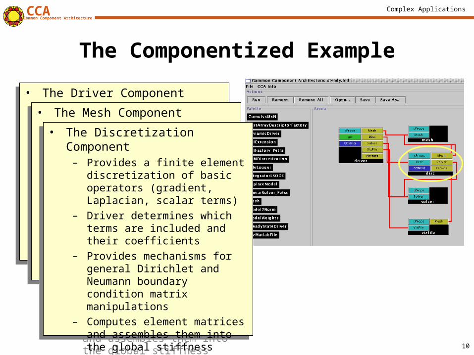
• The Discretization Component– Provides a finite element
discretization of basic operators (gradient, Laplacian, scalar terms)
– Driver determines which terms are included and their coefficients
– Provides mechanisms for general Dirichlet and Neumann boundary condition matrix manipulations
– Computes element matrices and assembles them into the global stiffness matrix via set methods on the solver
– Gathers and scatters vectors to the mesh (in this case )
Complex Applications CCACommon Component Architecture
11
The Componentized Example
• The Driver Component – Responsible for the overall
application flow– Initializes the mesh, discretization,
solver and visualization components
– Sets the physics parameters and boundary condition information
• The Driver Component – Responsible for the overall
application flow– Initializes the mesh, discretization,
solver and visualization components
– Sets the physics parameters and boundary condition information
• The Mesh Component– Provides geometry and topology
information– Provides the ability to attach user
defined data to mesh entities– Is used by the driver,
discretization and visualization components
• The Mesh Component– Provides geometry and topology
information– Provides the ability to attach user
defined data to mesh entities– Is used by the driver,
discretization and visualization components
• The Discretization Component– Provides a finite element
discretization of basic operators (gradient, laplacian, scalar terms)
– Provides mechanisms for general Dirichlet and Neumann boundary condition manipulations
– Computes element matrices and assembles them into the global stiffness matrix via set methods on the solver
– Gathers and scatters vectors to the mesh (in this case )
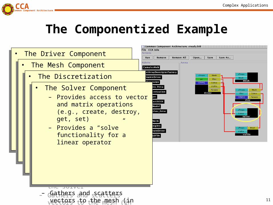
• The Solver Component– Provides access to vector and
matrix operations (e.g., create, destroy, get, set)
– Provides a “solve” functionality for a linear operator
• The Solver Component– Provides access to vector and
matrix operations (e.g., create, destroy, get, set)
– Provides a “solve” functionality for a linear operator
Complex Applications CCACommon Component Architecture
12
The Componentized Example
• The Driver Component – Responsible for the overall
application flow– Initializes the mesh, discretization,
solver and visualization components
– Sets the physics parameters and boundary condition information
• The Driver Component – Responsible for the overall
application flow– Initializes the mesh, discretization,
solver and visualization components
– Sets the physics parameters and boundary condition information
• The Mesh Component– Provides geometry and topology
information– Provides the ability to attach user
defined data to mesh entities– Is used by the driver,
discretization and visualization components
• The Mesh Component– Provides geometry and topology
information– Provides the ability to attach user
defined data to mesh entities– Is used by the driver,
discretization and visualization components
• The Discretization Component– Provides a finite element
discretization of basic operators (gradient, laplacian, scalar terms)
– Provides mechanisms for general Dirichlet and Neumann boundary condition manipulations
– Computes element matrices and assembles them into the global stiffness matrix via set methods on the solver
– Gathers and scatters vectors to the mesh (in this case )
• The Discretization Component– Provides a finite element
discretization of basic operators (gradient, laplacian, scalar terms)
– Provides mechanisms for general Dirichlet and Neumann boundary condition manipulations
– Computes element matrices and assembles them into the global stiffness matrix via set methods on the solver
– Gathers and scatters vectors to the mesh (in this case )
• The Solver Component– Provides access to vector and
matrix operations (e.g., create, destroy, get, set)
– Provides a “solve” functionality for a linear operator
• The Solver Component– Provides access to vector and
matrix operations (e.g., create, destroy, get, set)
– Provides a “solve” functionality for a linear operator
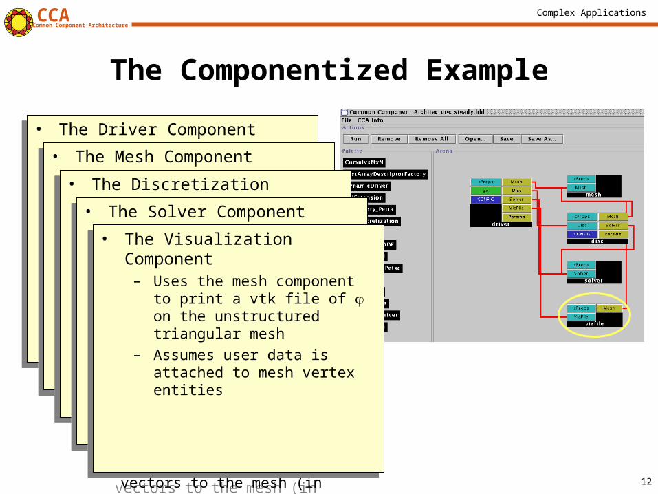
• The Visualization Component– Uses the mesh component to print
a vtk file of on the unstructured triangular mesh
– Assumes user data is attached to mesh vertex entities
• The Visualization Component– Uses the mesh component to print
a vtk file of on the unstructured triangular mesh
– Assumes user data is attached to mesh vertex entities
Complex Applications CCACommon Component Architecture
13
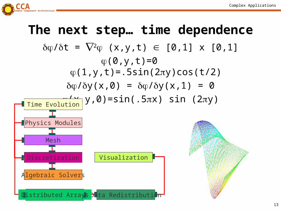
The next step… time dependence/t = 2 (x,y,t) [0,1] x [0,1]
(0,y,t)=0 (1,y,t)=.5sin(2y)cos(t/2)
/y(x,0) = /y(x,1) = 0
(x,y,0)=sin(.5x) sin (2y)
Time Evolution
Discretization
Algebraic Solvers
Mesh
Physics Modules
Visualization
Data RedistributionDistributed Arrays
Complex Applications CCACommon Component Architecture
14
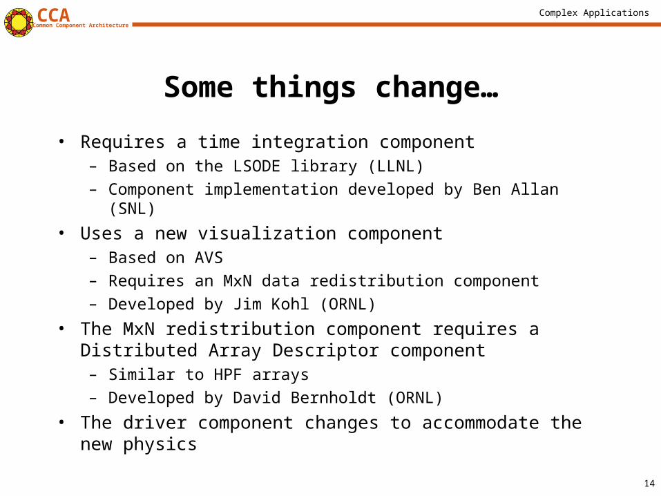
Some things change…
• Requires a time integration component– Based on the LSODE library (LLNL)
– Component implementation developed by Ben Allan (SNL)
• Uses a new visualization component– Based on AVS
– Requires an MxN data redistribution component
– Developed by Jim Kohl (ORNL)
• The MxN redistribution component requires a Distributed Array Descriptor component– Similar to HPF arrays
– Developed by David Bernholdt (ORNL)
• The driver component changes to accommodate the new physics
Complex Applications CCACommon Component Architecture
15
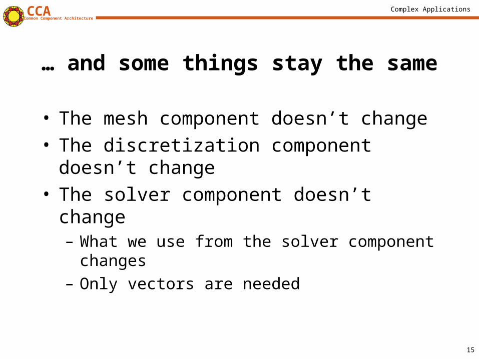
… and some things stay the same
• The mesh component doesn’t change• The discretization component doesn’t change• The solver component doesn’t change
– What we use from the solver component changes– Only vectors are needed
Complex Applications CCACommon Component Architecture
16
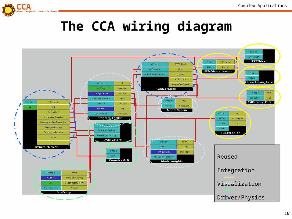
The CCA wiring diagram
Reused Integration Visualization Driver/Physics
Complex Applications CCACommon Component Architecture
17
What did this exercise teach us?
• It was easy to incorporate the functionalities of components developed at other labs and institutions given a well-defined interface and header file.– In fact, some components (one uses and one provides) were
developed simultaneously across the country from each other after the definition of a header file.
– Amazingly enough, they usually “just worked” when linked together (and debugged individually).
• In this case, the complexity of the component-based approach was higher than the original code complexity.– Partially due to the simplicity of this example– Partially due to the limitations of the some of the current
implementations of components
Complex Applications CCACommon Component Architecture
18
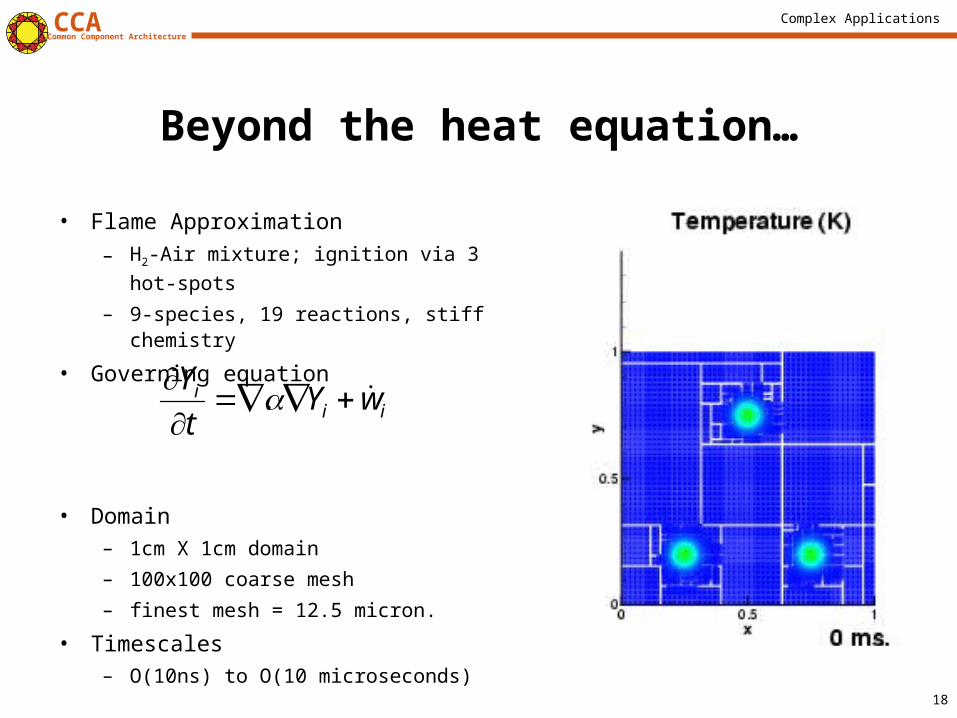
Beyond the heat equation…
• Flame Approximation
– H2-Air mixture; ignition via 3 hot-spots
– 9-species, 19 reactions, stiff chemistry
• Governing equation
• Domain– 1cm X 1cm domain
– 100x100 coarse mesh
– finest mesh = 12.5 micron.
• Timescales – O(10ns) to O(10 microseconds)
iii wYt
Y .
Complex Applications CCACommon Component Architecture
19
Numerical Solution
• Adaptive Mesh Refinement: GrACE• Stiff integrator: CVODE (LLNL)• Diffusive integrator: 2nd Order Runge Kutta• Chemical Rates: legacy f77 code (SNL)• Diffusion Coefficients: legacy f77 code (SNL) • New code less than 10%
Complex Applications CCACommon Component Architecture
20
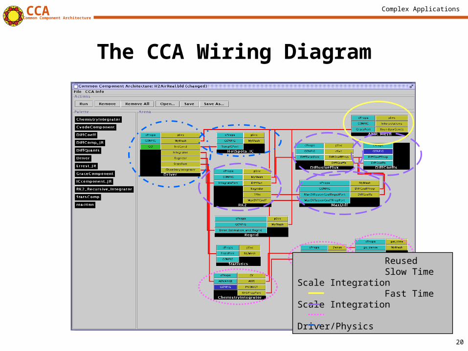
The CCA Wiring Diagram
Reused Slow Time Scale Integration Fast Time Scale Integration Driver/Physics
Complex Applications CCACommon Component Architecture
21
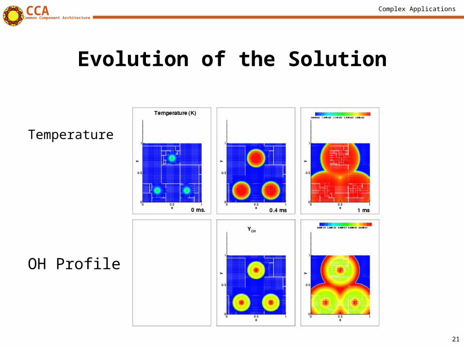
Evolution of the Solution
Temperature
OH Profile
Complex Applications CCACommon Component Architecture
22
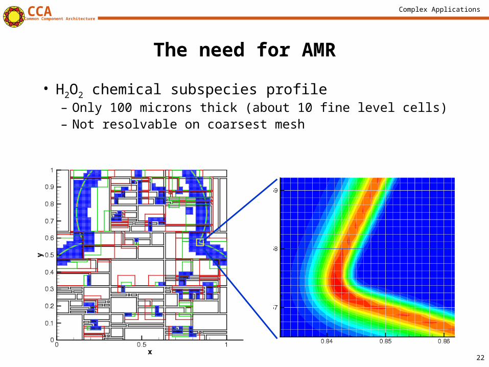
The need for AMR
• H2O2 chemical subspecies profile– Only 100 microns thick (about 10 fine level cells)– Not resolvable on coarsest mesh
Complex Applications CCACommon Component Architecture
23
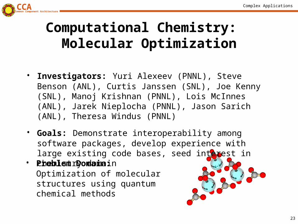
Computational Chemistry: Molecular Optimization
• Problem Domain: Optimization of molecular structures using quantum chemical methods
• Investigators: Yuri Alexeev (PNNL), Steve Benson (ANL), Curtis Janssen (SNL), Joe Kenny (SNL), Manoj Krishnan (PNNL), Lois McInnes (ANL), Jarek Nieplocha (PNNL), Jason Sarich (ANL), Theresa Windus (PNNL)
• Goals: Demonstrate interoperability among software packages, develop experience with large existing code bases, seed interest in chemistry domain
Complex Applications CCACommon Component Architecture
24
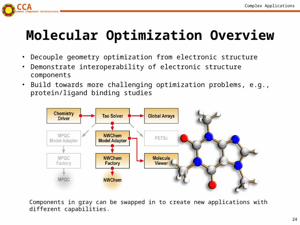
Molecular Optimization Overview
• Decouple geometry optimization from electronic structure• Demonstrate interoperability of electronic structure components• Build towards more challenging optimization problems, e.g.,
protein/ligand binding studies
Components in gray can be swapped in to create new applications with different capabilities.
Complex Applications CCACommon Component Architecture
25
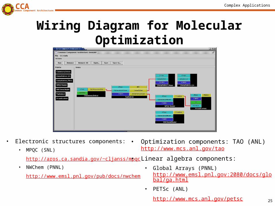
Wiring Diagram for Molecular Optimization
• Electronic structures components:
• MPQC (SNL)
http://aros.ca.sandia.gov/~cljanss/mpqc
• NWChem (PNNL)
http://www.emsl.pnl.gov/pub/docs/nwchem
• Optimization components: TAO (ANL) http://www.mcs.anl.gov/tao
• Linear algebra components:
• Global Arrays (PNNL) http://www.emsl.pnl.gov:2080/docs/global/ga.html
• PETSc (ANL)
http://www.mcs.anl.gov/petsc
Complex Applications CCACommon Component Architecture
26
Molecular Optimization Summary
• CCA Impact– Demonstrated unprecedented interoperability in a
domain not known for it– Demonstrated value of collaboration through
components– Gained experience with several very different
styles of “legacy” code
• Future Plans– Extend to more complex optimization problems– Extend to deeper levels of interoperability
Complex Applications CCACommon Component Architecture
27
Componentized Climate Simulations
• NASA’s ESMF project has a component-based design for Earth system simulations– ESMF components can be assembled and run in CCA compliant
frameworks such as Ccaffeine.
• Zhou et al (NASA Goddard) has integrated a simple coupled Atmosphere-Ocean model into Ccaffeine and is working on the Cane-Zebiak model, well-known for predicting El Nino events.
• Different PDEs for ocean and atmosphere, different grids and time-stepped at different rates.– Synchronization at ocean-atmosphere interface; essentially,
interpolations between meshes– Ocean & atmosphere advanced in sequence
• Intuitively : Ocean, Atmosphere and 2 coupler components– 2 couplers : atm-ocean coupler and ocean-atm coupler.– Also a Driver / orchestrator component.
Complex Applications CCACommon Component Architecture
28
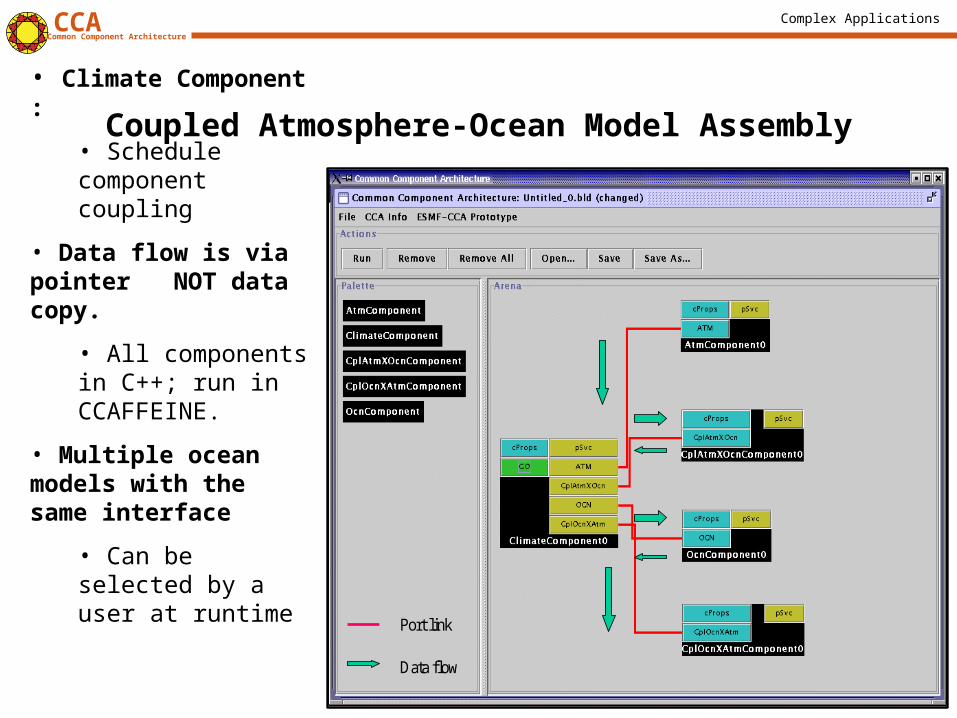
Coupled Atmosphere-Ocean Model Assembly
Data flow
Port link
• Climate Component :
• Schedule component coupling
• Data flow is via pointer NOT data copy.
• All components in C++; run in CCAFFEINE.
• Multiple ocean models with the same interface
• Can be selected by a user at runtime
Complex Applications CCACommon Component Architecture
29
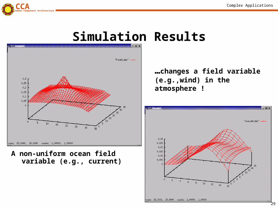
Simulation Results
A non-uniform ocean field variable (e.g., current)
…changes a field variable (e.g.,wind) in the atmosphere !
Complex Applications CCACommon Component Architecture
30
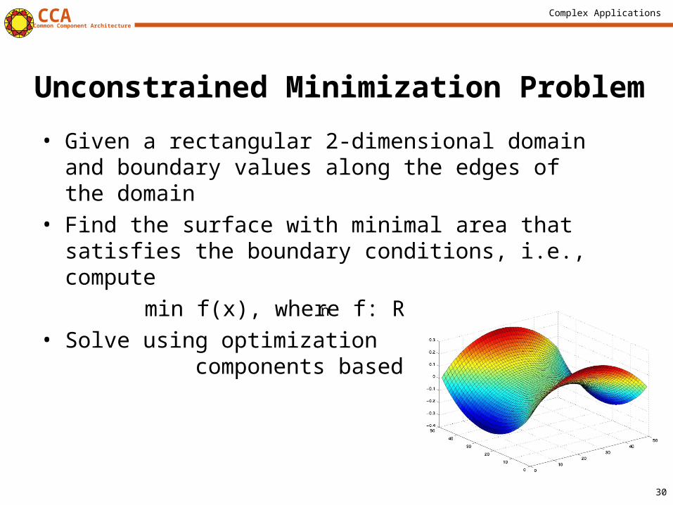
• Given a rectangular 2-dimensional domain and boundary values along the edges of the domain
• Find the surface with minimal area that satisfies the boundary conditions, i.e., compute
min f(x), where f: R R• Solve using optimization
components based on TAO (ANL)
Unconstrained Minimization Problem
n
Complex Applications CCACommon Component Architecture
31
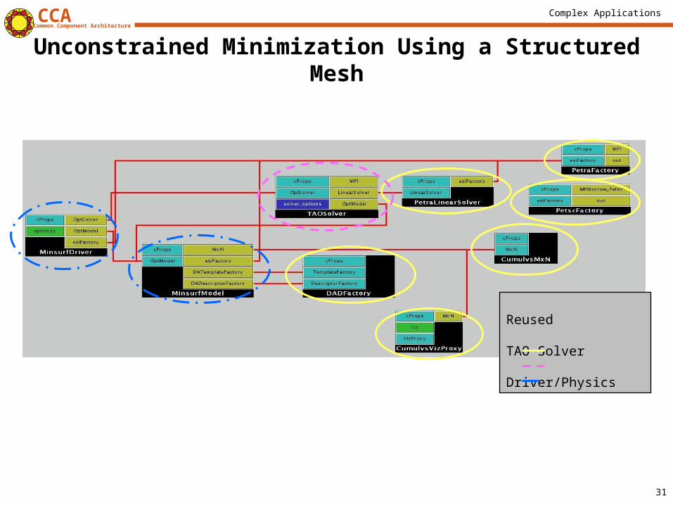
Unconstrained Minimization Using a Structured Mesh
Reused TAO Solver Driver/Physics
Complex Applications CCACommon Component Architecture
32
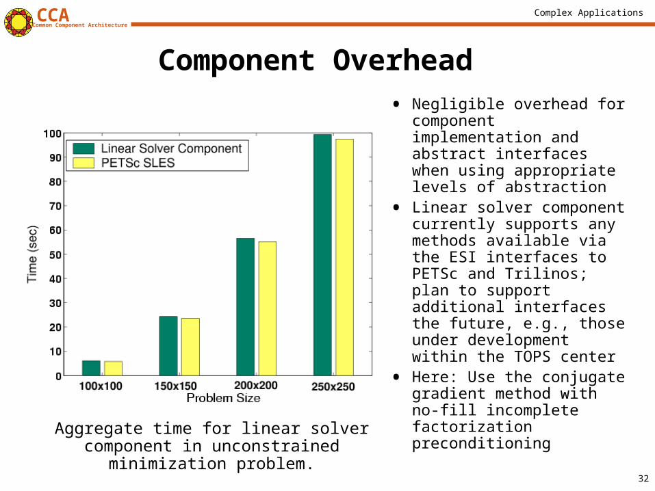
Component Overhead
• Negligible overhead for component implementation and abstract interfaces when using appropriate levels of abstraction
• Linear solver component currently supports any methods available via the ESI interfaces to PETSc and Trilinos; plan to support additional interfaces the future, e.g., those under development within the TOPS center
• Here: Use the conjugate gradient method with no-fill incomplete factorization preconditioning
Aggregate time for linear solver component in unconstrained minimization problem.
Complex Applications CCACommon Component Architecture
33
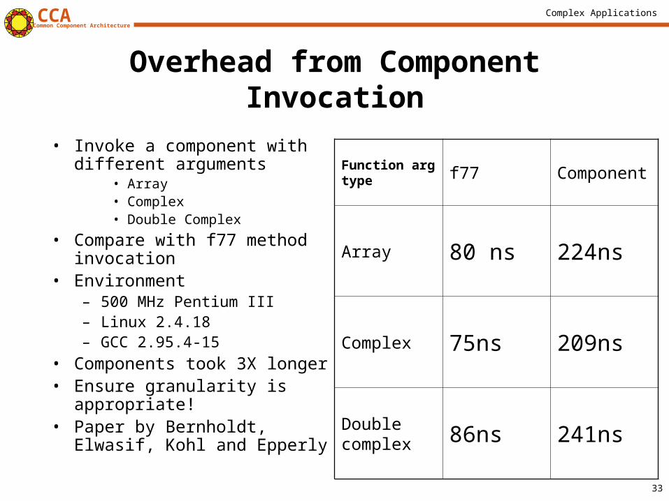
Overhead from Component Invocation
• Invoke a component with different arguments
• Array• Complex• Double Complex
• Compare with f77 method invocation
• Environment– 500 MHz Pentium III– Linux 2.4.18– GCC 2.95.4-15
• Components took 3X longer• Ensure granularity is
appropriate!• Paper by Bernholdt, Elwasif,
Kohl and Epperly
Function arg type f77 Component
Array 80 ns 224ns
Complex 75ns 209ns
Double complex 86ns 241ns
Complex Applications CCACommon Component Architecture
34
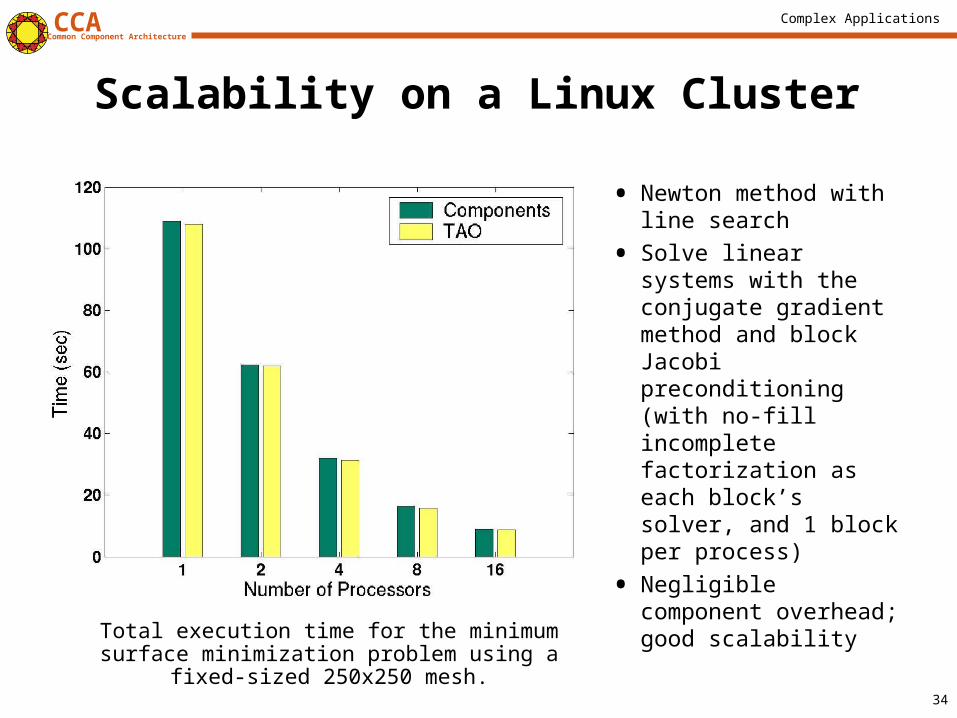
Scalability on a Linux Cluster
• Newton method with line search
• Solve linear systems with the conjugate gradient method and block Jacobi preconditioning (with no-fill incomplete factorization as each block’s solver, and 1 block per process)
• Negligible component overhead; good scalabilityTotal execution time for the minimum surface minimization
problem using a fixed-sized 250x250 mesh.
Complex Applications CCACommon Component Architecture
35
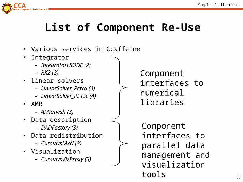
List of Component Re-Use
• Various services in Ccaffeine• Integrator
– IntegratorLSODE (2)– RK2 (2)
• Linear solvers– LinearSolver_Petra (4)– LinearSolver_PETSc (4)
• AMR– AMRmesh (3)
• Data description– DADFactory (3)
• Data redistribution– CumulvsMxN (3)
• Visualization– CumulvsVizProxy (3)
Component interfaces to parallel data management and visualization tools
Component interfaces to numerical libraries
Complex Applications CCACommon Component Architecture
36
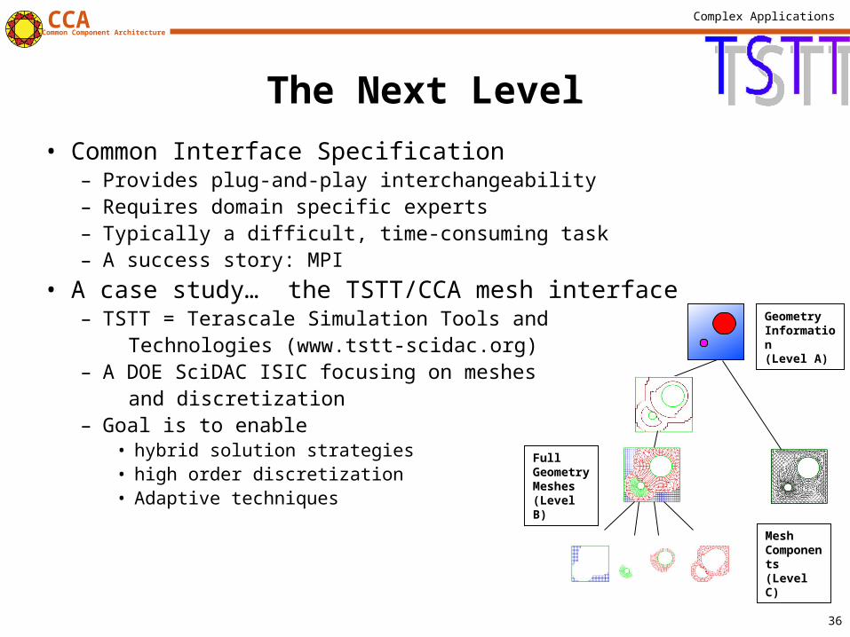
The Next Level
• Common Interface Specification– Provides plug-and-play interchangeability– Requires domain specific experts– Typically a difficult, time-consuming task– A success story: MPI
• A case study… the TSTT/CCA mesh interface– TSTT = Terascale Simulation Tools and Technologies (www.tstt-scidac.org)– A DOE SciDAC ISIC focusing on meshes and discretization– Goal is to enable
• hybrid solution strategies• high order discretization• Adaptive techniques
GeometryInformation(Level A)
Full GeometryMeshes(Level B)
MeshComponents(Level C)
Complex Applications CCACommon Component Architecture
37
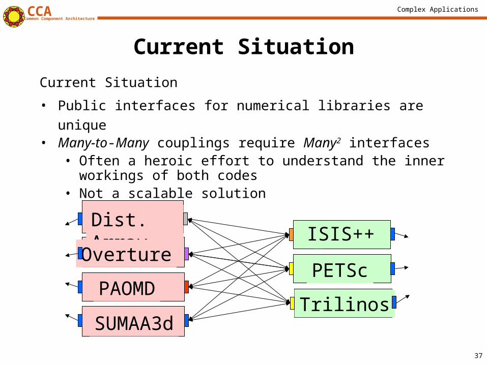
Current Situation
Current Situation
• Public interfaces for numerical libraries are unique• Many-to-Many couplings require Many2 interfaces
• Often a heroic effort to understand the inner workings of both codes
• Not a scalable solution
Dist. Array
Overture
PAOMD
SUMAA3d
PETSc
ISIS++
Trilinos
Complex Applications CCACommon Component Architecture
38
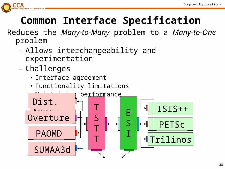
Common Interface SpecificationReduces the Many-to-Many problem to a Many-to-One problem
– Allows interchangeability and experimentation– Challenges
• Interface agreement• Functionality limitations• Maintaining performance
Dist. Array
Overture
PAOMD
SUMAA3d
ISIS++
PETSc
Trilinos
TSTT
ESI
Complex Applications CCACommon Component Architecture
39
TSTT Philosophy
Create a small set of interfaces that existing packages can support
AOMD, CUBIT, Overture, GrACE, …Enable both interchangeability and interoperability
Balance performance and flexibilityWork with a large tool provider and application community to ensure applicability
Tool providers: TSTT and CCA SciDAC centersApplication community: SciDAC and other DOE applications
Complex Applications CCACommon Component Architecture
40
Basic Interface
• Enumerated types– Entity Type: VERTEX, EDGE, FACE, REGION
– Entity Topology: POINT, LINE, POLYGON, TRIANGLE, QUADRILATERAL, POLYHEDRON, TETRAHEDRON, HEXAHEDRON, PRISM, PYRAMID, SEPTAHEDRON
• Opaque Types– Mesh, Entity, Workset, Tag
• Required interfaces– Entity queries (geometry, adjacencies), Entity iterators,
Array-based query, Workset iterators, Mesh/Entity Tags, Mesh Services
Complex Applications CCACommon Component Architecture
41
Issues that have arisen• Nomenclature is harder than we first thought• Cannot achieve the 100 percent solution, so...
– What level of functionality should be supported?• Minimal interfaces only?• Interfaces for convenience and performance?
– What about support of existing packages? • Are there atomic operations that all support?• What additional functionalities from existing packages should be required?
– What about additional functionalities such as locking?
• Language interoperability is a problem– Most TSTT tools are in C++, most target applications are in Fortran– How can we avoid the “least common denominator” solution?– Exploring the SIDL/Babel language interoperability tool
Complex Applications CCACommon Component Architecture
42
Summary
• Complex applications that use components are possible– Combustion– Chemistry applications– Optimization problems– Climate simulations
• Component reuse is significant– Adaptive Meshes– Linear Solvers (PETSc, Trilinos)– Distributed Arrays and MxN Redistribution– Time Integrators– Visualization
• Examples shown here leverage and extend parallel software and interfaces developed at different institutions
– Including CUMULVS, ESI, GrACE, LSODE, MPICH, PAWS, PETSc, PVM, TAO, Trilinos, TSTT.
• Performance is not significantly affected by component use• Definition of domain-specific common interfaces is key
Complex Applications CCACommon Component Architecture
43
Componentizing your own application
• The key step: think about the decomposition strategy– By physics module?– Along numerical solver functionality?– Are there tools that already exist for certain pieces? (solvers,
integrators, meshes?)– Are there common interfaces that already exist for certain pieces? – Be mindful of the level of granularity
• Decouple the application into pieces– Can be a painful, time-consuming process
• Incorporate CCA-compliance• Compose your new component application• Enjoy!