arX

iv:h

ep-p

h/04

0809

8v1

6 A

ug 2

004

Z ′ Gauge Bosons at the Tevatron

Marcela Carena1, Alejandro Daleo1,2 Bogdan A. Dobrescu1, Tim M.P. Tait1

1 Theoretical Physics Department, Fermilab, Batavia, IL 60510, USA

2 Departamento de Fısica, Universidad Nacional de La Plata,

C.C. 67-1900 La Plata, Argentina.

August 5, 2004

FERMILAB-Pub-04/129-T

hep-ph/0408098

Abstract

We study the discovery potential of the Tevatron for a Z ′ gauge boson. Weintroduce a parametrization of the Z ′ signal which provides a convenient bridgebetween collider searches and specific Z ′ models. The cross section for pp → Z ′X →ℓ+ℓ−X depends primarily on the Z ′ mass and the Z ′ decay branching fraction intoleptons times the average square coupling to up and down quarks. If the quark andlepton masses are generated as in the standard model, then the Z ′ bosons accessibleat the Tevatron must couple to fermions proportionally to a linear combination ofbaryon and lepton numbers in order to avoid the limits on Z − Z ′ mixing. Moregenerally, we present several families of U(1) extensions of the standard model thatinclude as special cases many of the Z ′ models discussed in the literature. Typically,the CDF and D0 experiments are expected to probe Z ′-fermion couplings downto 0.1 for Z ′ masses in the 500–800 GeV range, which in various models wouldsubstantially improve the limits set by the LEP experiments.

1 Introduction

An important question in particle physics today is whether there are any new gauge

bosons beyond the ones associated with the SU(3)C × SU(2)W × U(1)Y gauge group.

This question is interesting by itself, given that the selection of the gauge bosons observed

so far remains mysterious. Furthermore, new gauge bosons are predicted within many

theories beyond the Standard Model (SM) which have been developed to provide answers

to its many open questions.

The simplest way of extending the SM gauge structure is to include a second U(1)

group. The associated gauge boson, usually labeled Z ′, is an electrically-neutral spin-1

particle. If the new gauge coupling is not much smaller than unity, then the U(1) group

must be spontaneously broken at a scale larger than the electroweak scale in order to

account for the nonobservation of the Z ′ boson at LEP and run I of the Tevatron. In

this article, we study the Z ′ discovery potential of the run II of the Tevatron, the highest

energy hadron machine operating for the next few years.

The theoretical framework for studying Z ′ production at hadron colliders has been

developed more than two decades ago [1]. Nevertheless, various pieces of information

collected recently have an impact on our attempt of addressing a number of specific

questions: What Z ′ parameters are relevant for Tevatron searches? What regions of the

parameter space are not ruled out by the LEP experiments, and would allow a Z ′ discovery

at the Tevatron? In case of a discovery, how can one differentiate between the models

that may accommodate a Z ′ boson?

It is often assumed that the Z ′ couplings have certain values motivated by some

narrow theoretical assumptions, allowing for the derivation of a Z ′ mass bound [2, 3].

The opposite approach of leaving the couplings arbitrary [4] suffers from the existence of

too many free parameters. However, a few theoretical constraints are sufficiently generic

so that it is reasonable to focus on the region of the parameter space that satisfies them.

This observation, used to define the so-called nonexotic Z ′ bosons [5], underscores the

importance of the Z ′ couplings to the SM fermions for collider phenomenology [6], while

reducing the set of Z ′ parameters.

In this article, we address Z ′ models both from a theoretical perspective and with

respect to their potential observation at hadron colliders. In Section 2 we present the

theoretical framework needed to describe a new neutral gauge boson. We analyze the

constraints due to gauge anomaly cancellation and the gauge invariance of the quark

1

and lepton Yukawa couplings, and discuss what new physics would soften these con-

straints. We identify several interesting families of Z ′ models, and then derive the LEP

limits. Section 3 is concerned with Z ′ production at hadron colliders, including a survey

of theoretical tools to describe Z ′ events, and a convenient parameterization of limits

from searches that simplifies comparison of experimental results with theoretical models.

Section 4 summarizes our conclusions.

2 Parameters Describing New Neutral Gauge Bosons

Any new gauge boson is characterized by a mass and a number of coupling constants. All

these parameters appear in the Lagrangian, which is constrained by gauge and Lorentz

invariance. In this section we present a theoretical framework that is sufficiently general

to account for the parameters that are relevant for Z ′ searches at the Tevatron. We

discuss the theoretical constraints within realistic extensions of the SM, and then discuss

the LEP limits.

2.1 Z ′ mass and Z − Z ′ mixing

Consider the SM gauge symmetry extended by one Abelian gauge group, SU(3)C ×SU(2)W × U(1)Y × U(1)z. The scalar sector responsible for the spontaneous breaking

of the gauge symmetry down to SU(3)C×U(1)em

includes at least one Higgs doublet and

an SU(2)W singlet, φ, with VEV vφ. As we will explicitly show below, the constraints

on the interactions of the U(1)z gauge boson with quarks and leptons are relaxed in the

presence of two Higgs doublets, H1 and H2, with aligned VEVs vH1and vH2

. To be gen-

eral, we will concentrate on this case in what follows. The hypercharges of H1, H2, and

φ are given by +1, +1 and 0, respectively, so that electric charge is conserved.

In a basis where the three electrically neutral gauge bosons, W 3µ, BµY and Bµ

Z , have

diagonal kinetic terms, their mass terms are given by:

v2H1

8

(

gW 3µ − gYBµY − zH1

gzBµz

)2+v2H2

8

(

gW 3µ − gYBµY − zH2

gzBµz

)2+v2φ

8(zφgzB

µz )

2 ,

(2.1)

where g, gY , gz are the SU(2)W × U(1)Y × U(1)z gauge couplings, and the weak mixing

angle is given as usual by tan θw = gY /g. The diagonalization of these mass terms yields

the three physical states, the photon (labeled by Aµ), the observed Z boson, and the

2

hypothetical Z ′ boson:

Aµ = W 3µ sin θw +BµY cos θw ,

Zµ = W 3µ cos θw −BµY sin θw + ǫBµ

z ,

Z ′µ = Bµ

z − ǫ(

W 3µ cos θw −BµY sin θw

)

. (2.2)

To obtain this result we have ignored terms of order ǫ2, where ǫ is the mixing angle

between the SM Z boson and Bµz ,

ǫ =δM2

ZZ′

M2Z′ −M2

Z

. (2.3)

The mass-squared parameters introduced here are related to the VEVs by

M2Z =

g2

4 cos2 θw

(

v2H1

+ v2H2

) [

1 +O(

ǫ2)]

,

M2Z′ =

g2z

4

(

z2H1v2H1

+ z2H2v2H2

+ z2φv

2φ

) [

1 +O(

ǫ2)]

,

δM2ZZ′ = − ggz

4 cos θw

(

zH1v2H1

+ zH2v2H2

)

. (2.4)

MZ and MZ′ are the physical masses of the neutral gauge bosons up to corrections of

order ǫ2.

A Z ′ boson which mixes with the SM Z distorts its properties, such as couplings to

fermions and mass relative to electroweak inputs. Precision measurements of observables,

mostly on the Z pole at LEP I and SLC, have verified the SM Z properties at or below

the per mil level1 [7], imposing a severe upper bound [8] on the mixing angle between the

Z and Z ′: |ǫ| ∼< 10−3. Therefore, it is justified to treat the mixing as a perturbation as

was done above.

From Eqs. (2.3) and (2.4) it follows that the mixing angle is given by

|ǫ| ≈ gzg

(

cos θwM2

Z′/M2Z − 1

) |zH1+ zH2

tan2β|1 + tan2β

(2.5)

where tan β = vH2/vH1

. At least one of vH1or vH2

has to be of the order of the electroweak

scale (to generate MW , MZ and mt appropriately), so without loss of generality we can

1The notable exception is sin2 θW from hadronic Z decays, which deviates at the few σ level [7], andplays an interesting role in the fit to the SM Higgs mass [9]. These deviations have been argued asevidence for the existence of a Z ′ with non-universal interactions [10]; we shall not pursue this line ofreasoning here.

3

set vH2∼ O(246) GeV. Therefore, tan β ∼> O(1). Normalizing the largest quark U(1)z

charges to be of order unity, the Z ′ production at the Tevatron is sizable only if the gauge

coupling gz is not much smaller than unity. The mass range typically interesting at the

Tevatron is roughly 0.2 TeV < MZ′ < 0.7 TeV. Based on these considerations we find

that the order of magnitude of the mixing angle is given by ǫ ∼ (zH1cot2β+zH2

)M2Z/M

2Z′.

The constraint |ǫ| ∼< 10−3 implies zH1cot2β + zH2

≪ 1. Although tan2 β could be close

to −zH1/zH2

, this would be a fine tuning, because the value of tan β is set by the Higgs

masses and self-interactions, and has no reason to be related to the ratio of Higgs charges.

Therefore, in the absence of fine-tuning, a Z ′ accessible at the Tevatron requires |zH2| ≪ 1

and either |zH1| ≪ 1 or tanβ ≫ 1. It is usually expected that the charges of various fields

are either all of the same order or vanish. Although exceptions exist, such as extra

dimensional models with brane kinetic terms [11] on the Higgs brane, which motivate

much a smaller effective charge for the Higgs than for the (bulk) fermions, we restrict

attention here to the following two cases:

zH2= 0 and zH1

= 0 (2.6)

or

zH2= 0 and tan β ∼> 10 . (2.7)

2.2 Couplings to fermions

The renormalizable interactions of the Z ′ boson with the SM fermions are described by

the following terms in the Lagrangian density:

∑

f

zfgzZ′µfγ

µf , (2.8)

where f = ejR, ljL, u

jR, d

jR, q

jL are the usual lepton and quark fields in the weak eigenstate

basis; ljL = (νjL, ejL) and qjL = (ujL, d

jL) are the SU(2)W doublet fermions. The index j

labels the three fermion generations. Altogether there are 15 fermion charges, zf .

The observed quark and lepton masses and mixings restrict these fermion charges, so

that certain gauge and Lorentz invariant terms can appear in the Lagrangian. In the SM,

the terms responsible for the charged fermion masses are

λdjk qjLd

kRH + λujk q

jLu

kRiσ2H

† + λejk lj

LekRH + h.c. , (2.9)

4

where j, k = 1, 2, 3 label the fermion generations, and λdjk, λujk, λ

ejk are Yukawa couplings.

In the two Higgs-doublet model described above, the Higgs doublet H is replaced by linear

combinations of H1 and H2.

As discussed in section 2.1, the Z ′ bosons relevant for Tevatron searches have small

mixing with the Z boson, which effectively implies that any Higgs doublet with a VEV

of order the electroweak scale is neutral under the U(1)z symmetry. In particular, if only

one Higgs doublet is present, then its U(1)z charge would have to vanish. Given that

the total charge of the quark mass terms shown in Eq. (2.9) has to be zero, the quark

masses and CKM elements may then be accommodated only if the quarks have generation

independent U(1)z charges, and zu = zd = zq, where zu and zd are the right-handed up-

and down-type quark charges, and zq is the left-handed quark doublet charge. One may

relax this condition in the two Higgs-doublet model if, for example, H2 couples to the

up-type quarks, while H1 couples to the down-type quarks, has nonzero charge, and tanβ

is large. In that case zd may be different from zu and zq, but one still needs to impose

zu = zq , (2.10)

so that the large top-quark mass may be generated.

We emphasize that we have derived this strong conclusion based on reasonable but not

infallible arguments. One loophole is that some of the terms in Eq. (2.9) may be replaced

by higher-dimensional operators such as qjLdkRH(φ/Mheavy)

p, where p is an integer and

Mheavy is the mass scale where this dimension-(4 + p) operator is generated. Since the

weak-singlet scalar φ has a nonzero charge under U(1)z, the relations between the various

quark charges may be changed. The higher-dimensional operators may be induced in a

renormalizable quantum field theory by the exchange of heavy fermions that have Yukawa

couplings to both the Higgs doublets and φ. Another loophole is that both Higgs doublets

may be charged under U(1)z if there is a fine-tuning as discussed in section 2.1, so that the

restrictions on quark charges would be again modified. Based on these considerations,

we will study in some detail the implications of Eq. (2.10), but we will also consider

departures from it.

We point out that generation dependent quark charges lead to flavor-changing cou-

plings of the Z ′ in the mass eigenstate basis, where the fermion mass matrices are diagonal.

Various experimental constraints from flavor-changing neutral current processes impose

severe constraints on such flavor-changing Z ′ couplings, unless MZ′ is so large that the

effects of such a Z ′ would be beyond the reach of even the LHC. To avoid these com-

5

plications we will avoid generation dependent quark charges in this paper. In practice

this does not restrict significantly the generality of our results because the Tevatron is

typically not very sensitive to Z ′ decaying into quarks, and the production cross section

depends only on an average quark charge. Therefore, altogether there are three quark

charges relevant in what follows: zu, zd, zq.

The masses of the electrically-charged leptons can be induced by the last term shown

in Eq. (2.9) even if the lepton z-charges are generation dependent. Moreover, no flavor-

changing neutral currents are induced in the lepton sector by Z ′ exchange. The lepton

mass terms impose, though, a relation between the left- and right-handed lepton z-charges:

zlj = zej, j = 1, 2, 3, or zlj − zej

= zH1in the two-Higgs doublet model with large tanβ.

As in the case of the quarks, we allow for deviations from these equalities motivated by

lepton mass generation via higher-dimensional operators. Thus, all six lepton charges,

zlj , zej, j = 1, 2, 3 could be relevant for Tevatron studies.

Additional constraints arise due to the requirement of generating neutrino masses and

mixings. The terms in the Lagrangian responsible for these are given by

cjkMν

lcj

LlkLH

⊤iσ2H + λνjk′ lj

Liσ2νk′

RH† +mν

j′k′νcj

′

Rνk′

R + h.c. , (2.11)

where we have included right-handed neutrinos, νj′

R , which are singlets under the SM

gauge group. If these are not present, then the last two terms in the above equation

vanish. If there are n right-handed neutrino flavors, then j′, k′ = 1, ..., n. For n ≥ 2 all

dimensionless coefficients cjk of the above lepton-number-violating terms may vanish. The

other parameters appearing in Eq. (2.11) are as follows: Mν is the mass scale where the

lepton-number-violating terms are generated, mνj′k′ are right-handed neutrino Majorana

masses, λνjk′ are some Yukawa couplings.

The requirement that the three active neutrinos mix, so that the observed neutrino

oscillations can be accommodated, implies that the lepton charges are generation inde-

pendent. However, as in the case of quarks, the terms in Eq. (2.11) may be replaced

by higher-dimensional operators involving powers of φ/Mheavy. Furthermore, the tiny

neutrino masses make the existence of such higher-dimensional operators an attractive

possibility [5]. If several φ scalars carry different U(1)z charges, one could avoid almost

entirely the constraints from neutrino mixing on lepton charges.

The six lepton charges determine the leading decay width of the Z ′ into the corre-

6

sponding leptons:

Γ(Z ′ → e+j e−j ) ≈ (z2

lj+ z2

ej)g2z

24πMZ′ ,

Γ(Z ′ → νLνL) ≈(

z2l1 + z2

l2 + z2l3

) g2z

24πMZ′ , (2.12)

where ej = {e, µ, τ} for j = 1, 2, 3. Similarly, the quarks charges determine the following

decay widths of the Z ′:

Γ(Z ′ → jets) ≈ (2z2q + z2

u + z2d)g2z

4πMZ′

(

1 +αsπ

)

,

Γ(Z ′ → bb) ≈ (z2q + z2

d)g2z

8πMZ′

(

1 +αsπ

)

,

Γ(Z ′ → tt) ≈ (z2q + z2

u)g2z

8πMZ′

(

1 − m2t

M2Z′

)(

1 − 4m2t

M2Z′

)1/2

×[

1 +αsπ

+O(

αsm2t/M

2Z′

)

]

θ (MZ′ − 2mt) . (2.13)

where “jets” refers to hadrons not containing bottom or top quarks and we have included

the leading QCD corrections, but we have ignored electroweak corrections and all fermion

masses with the exception of the top-quark mass, mt. Additional decay modes, into pairs

of Higgs bosons (if zH16= 0 or zH2

6= 0), CP-even components of the φ scalar, right-handed

neutrinos, or other new particles might be kinematically accessible and large. Therefore,

the total decay width, ΓZ′, is larger than or equal to the sum of the seven decay widths

shown in Eqs. (2.12) and (2.13).

Assuming that the decays into particles other than the SM fermions are either invisible

or have negligible branching ratios, the Z ′ properties depend primarily on eleven param-

eters: mass (MZ′), total width (ΓZ′), and nine fermion couplings (zej, zlj , zq, zu, zd)×gz.

2.3 Realistic models

So far we have imposed SU(3)C × SU(2)W × U(1)Y × U(1)z gauge invariance on the La-

grangian. Additional restrictions need to be imposed in order to preserve gauge invariance

in the full quantum field theory: the fermion content of the theory has to be such that

all gauge anomalies cancel. In our case, we need to make sure that there are no gauge

anomalies due to triangle diagrams with gauge bosons as external lines.

7

Triangle diagrams involving two gluons or two SU(2)W gauge bosons, and one U(1)z

gauge bosons give rise to the [SU(3)C ]2U(1)z and [SU(2)W ]2U(1)z anomalies:

A33z = 3 (2zq − zu − zd) ,

A22z = 9zq +3∑

j=1

zlj . (2.14)

Triangle diagrams involving U(1)Y × U(1)z gauge bosons give rise to the [U(1)Y ]2U(1)z,

U(1)Y [U(1)z]2 and [U(1)z]

3 anomalies:

A11z = 2zq − 16zu − 4zd + 2

3∑

j=1

(

zlj − 2zej

)

,

A1zz = 6(

z2q − 2z2

u + z2d

)

− 2

3∑

j=1

(

z2lj− z2

ej

)

,

Azzz = 9(

2z3q − z3

u − z3d

)

+

3∑

j=1

(

2z3lj− z3

ej

)

−n∑

i=1

z3νi, (2.15)

where we have included n right-handed neutrinos of charges zνiunder U(1)z. Finally,

triangle diagrams involving two gravitons and one U(1)z gauge boson contribute to the

mixed gravitational-U(1)z anomaly, which makes general coordinate invariance incompat-

ible with U(1)z gauge invariance:

AGGz = 9 (2zq − zu − zd) +

3∑

j=1

(

2zlj − zej

)

−n∑

i=1

zνi(2.16)

Gauge invariance at quantum level requires that all the anomalies listed in Eqs. (2.14)-

(2.16) vanish, or are exactly canceled by anomalies associated with some new fermions

charged under both the SM gauge group and U(1)z. The impact of the new fermions on the

Z ′ properties described here can be ignored if they are heavier than the Z ′. Altogether,

there are six equations that restrict the nine z-charges of the SM fermions. Finding

solutions to this set of equations is a nontrivial task, especially if one imposes that the

charges are rational numbers, as suggested by grand unified theories.

The case where the top-quark mass is generated by a Yukawa coupling to a Higgs

doublet, as in the SM or the Minimal Supersymmetric Standard Model (MSSM), leads to

8

Eq. (2.10), in which case the A33z , A22z and A11z anomalies vanish only if

zq = zu = zd = −1

9

3∑

j=1

zlj , (2.17)

3∑

j=1

(

zlj − zej

)

= 0 . (2.18)

The remaining anomaly cancellation conditions, in the absence of exotic fermions, take

the following form:

3∑

j=1

(

z2lj− z2

ej

)

= 0 ,

3∑

j=1

(

2z3lj− z3

ej

)

=n∑

i=1

z3νi

n∑

i=1

zνi= −9zq (2.19)

It is hard to find general solutions to this set of equations. A well known nontrivial

solution is n = 3 and zlj = zej= zνj

= zl, j = 1, 2, 3, which corresponds to the U(1)B−L

gauge group. The associated gauge boson, ZB−L, is an interesting case of a “non-exotic”

Z ′ [5] relevant for Tevatron searches. We have found a generalization of this solution

which preserves the zlj = zej= zνj

equalities within each generation, but have different

lepton charges for different generations. In particular, the case of zl1 = 0 is worth special

attention because the Z ′ does not couple to electrons, so there are no tight limits from

LEP. In this case there are only two independent charges: zq which sets all quark charges,

and zl2 which sets the charges of the muon and second-generation neutrinos. Normalizing

the gauge coupling such that zq = 1/3, the τ and third-generation neutrinos have charge

zl3 = −3 − zl2 . (2.20)

If new fermions are included, the anomaly cancellation conditions have more solutions.

We have found that including within each generation two fermions, ψl and ψe, which under

the SM gauge group are vector-like and have the same charges as lL and eR, respectively,

allows z charges proportional to B − xL with x arbitrary. The U(1)B−xL charges are

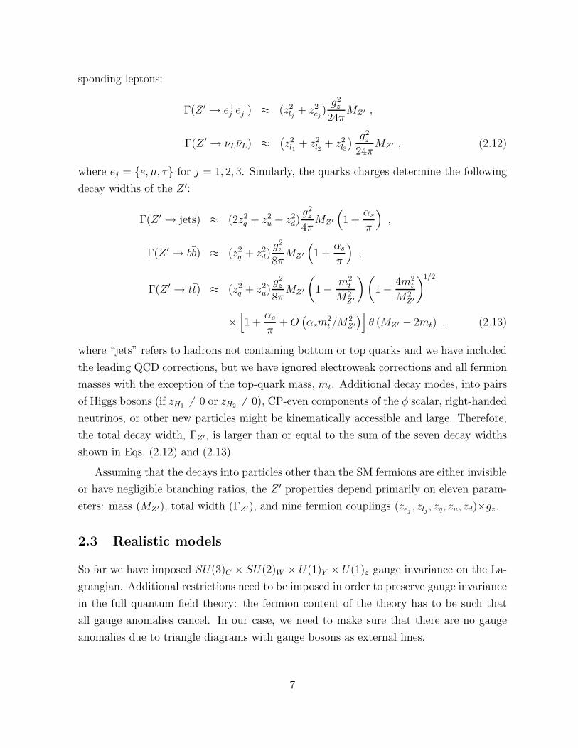
shown in Table 1. This is the most general generation-independent charge assignment

9

SU(3)C SU(2)W U(1)Y U(1)B−xL U(1)q+xu U(1)10+x5 U(1)d−xu

qL 3 2 1/3 1/3 1/3 1/3 0

uR 3 1 4/3 1/3 x/3 −1/3 −x/3dR 3 1 −2/3 1/3 (2 − x)/3 −x/3 1/3

lL 1 2 −1 −x −1 x/3 (−1 + x)/3

eR 1 1 −2 −x −(2 + x)/3 −1/3 x/3

νR −1 (−4 + x)/3 (−2 + x)/3 −x/31 1 0

ν ′R · · −1 − x/3 ·ψlL −1 · −(1 + x)/3 −2x/5

1 2 −1ψlR −x · 2/3 (−1 + x/5)/3

ψeL −1 · · ·1 1 −2

ψeR −x · · ·ψdL · · −2/3 (1 − 4x/5)/3

3 1 −2/3ψdR · · (1 + x)/3 x/15

Table 1: Fermion gauge charges.

for the SM fermions that allows quark and lepton masses from Yukawa couplings, and is

relevant for Z ′ searches at the Tevatron.

All other generation-independent U(1)z charge assignments require the restrictions

on fermion charges from fermion mass generation to be lifted, for example by replacing

the Yukawa couplings with higher-dimensional operators. The six anomalies given in

Eqs. (2.14)-(2.16) vanish only for the nonexotic family of U(1)z charges that depends on

two parameters [5]. Assuming that zq 6= 0, and normalizing the gz gauge coupling such

that zq = 1/3, determines all other charges as a linear function of a single free parameter,

x, as shown in Table 1. We label this charge assignment by U(1)q+xu. Particular cases

of Z ′ “models” include U(1)B−L for x = 1, the U(1)χ from SO(10) grand unification for

x = −1, and the [U(1)R × U(1)B−L]/U(1)Y group from left-right symmetric models for

x = 4 − 3g2R/g

2Y where gR is the U(1)R gauge coupling.

Many popular Z ′ models are accessible at the Tevatron provided both the restrictions

from fermion mass generation are lifted and new fermions charged under the SM gauge

group are present. We have found a couple of generation-independent charge assignments

10

that depend on a free parameter x, which include the E6-inspired Z ′ models that have been

frequently analyzed by experimental collaborations. Both require within each generation

two fermions, ψl and ψd, which under the SM gauge group are vector-like and have the

same charges as lL and dR, respectively. One assignment, labeled by U(1)d−xu, has zq = 0,

zd = 1/3 and zu = −x/3. For x = 0 the E6-inspired U(1)I is recovered, while x = 1

gives the “right-handed” U(1)R group. The other assignment is such that all fermions

belonging to the 10 representation of the SU(5) grand unified group have the same U(1)z

charge, assumed to be nonzero and normalized to 1/3, while the fermions belonging to

the 5 representation have charge x/3. We label this assignment by U(1)10+x5. Anomaly

cancellation requires two right-handed neutrinos per generation. Particular E6-inspired

cases include U(1)ψ for x = 1, U(1)χ for x = −3, and U(1)η for x = −1/2. Note that when

the LEP and Tevatron experimental collaborations refer to these particular models, the

gauge coupling is usually assumed to be determined by a unification relation: g2z = g2

Y ξ,

with ξ = 5/8 for U(1)ψ, ξ = 3/8 for U(1)χ, ξ = 1 for U(1)η, ξ = 5/3 for U(1)I . Thus, our

families of models completely describe the physics of the GUT-inspired U(1)’s, but also

allow one to relax their assumptions and explore more general Z ′ physics.

There is an interesting class of Z ′ models in which the Higgs is a pseudo-Goldstone

boson of a spontaneously broken global symmetry. These “Little Higgs” models always

include at least one Z ′ to cancel the leading quadratic divergence in the Higgs mass from

loops of the ordinary W and Z. A proto-typical model of this type is the “Littlest Higgs”

[12]. This already reveals a key feature of the little Higgs Z ′: it always couples to the

Higgs, and thus generically has strong constraints from Z-Z ′ mixing, requiring the Z ′

mass to be larger than several hundred GeV [13]. Thus, it is usually not very interesting

for Tevatron searches.

2.4 LEP II limits on Z ′ models

The constraints from e+e− colliders on the Z ′ properties fall into two categories: precision

measurements at the Z pole, through the Z-Z ′ mixing discussed previously, and measure-

ments of e+e− → f f above the Z-pole at LEP-II, where f are various SM fermions. In

practice, the agreement with the SM requires that either the Z ′ gauge coupling is smaller

than or of order 10−2 [5], or else MZ′ is larger than the largest collider energy of LEP-II,

of about 209 GeV. In the latter case, of interest at the Tevatron, one can perform an

expansion in s/M2Z′, where s is the square of the center-of-mass energy. This leads to

effective contact interactions which have been bounded by LEP-II for all possible chiral

11

structures and for various combinations of fermions. These interactions are parameterized

by the LEP electroweak working group [14] as,

±4π

(1 + δef)(Λf±AB)2

(eγµPAe)(

fγµPBf)

(2.21)

where PA is a projector for right- (A = R) or left-handed (A = L) chiral fields, and

δef = 1, 0 for f = e, f 6= e, respectively. These contact interactions provide a model-

independent framework in which LEP-II data can confront high mass effects beyond the

SM, up to corrections of order s/M2Z′.

In the absence of flavor violation in the Z ′ couplings, the Z ′ contributions to e+e− →f f for f 6= e proceed through an s-channel Z ′ exchange, with tree level matrix element,

g2z

M2Z′ − s

[eγµ(zlPL + zePR)e][

fγµ(zfLPL + zfR

PR)f]

(2.22)

where tiny terms of order mfme/M2Z′ have been dropped. In the case of f = e, there is

also a t-channel exchange, which in fact motivates the factor of (1 + δef) in Eq. (2.21),

which allows one to treat all f equivalently at the level of matrix elements.

One should compare the LEP ΛLL, ΛRR, ΛLR, and ΛRL limits to the operators of each

structure in the Z ′ theory in order to find a limit on a given Z ′ model. This procedure

finds the best single bound from each operator on a given Z ′ model, but it ignores the

potentially stronger bound that comes from the combined effect of more than one operator.

In the absence of a dedicated reanalysis of the data, this is the best one may do. However,

we reiterate that it does not always represent the best potential bound from the data,

due to correlated effects on observables which cannot be taken into account correctly in

this way. Typically the strongest bound comes from a single choice of chiral interaction

combination and f .

Matching the Z ′ matrix elements, Eq. (2.22), to the LEP-II formalism, Eq. (2.21), one

derives bounds such as,

M2Z′ − s ≥ g2

z

4π|zeA

zfB| (Λf±

AB)2 , (2.23)

and one must choose Λ+ for zeAzfB

> 0 or Λ− for zeAzfB

< 0. Typically, the LEP-II

bounds on the Λ’s are on the order of 10 TeV, schematically translating into bounds on

the Z ′ mass on the order of MZ′ ∼> |z|gz × (a few TeV). More precise bounds in the

case of certain models are discussed below. The Tevatron can effectively improve our

knowledge of Z ′ models only when the couplings zgz are appropriately small such that

12

0

2

4

6

8

10

12

14

16

18

20

-10 -8 -6 -4 -2 0 2 4 6 8 10

U(1)q+xu

LEP Bounds

U(1)10+x5

U(1)d-xu

U(1)B-xL

x

M /

g z (T

eV)

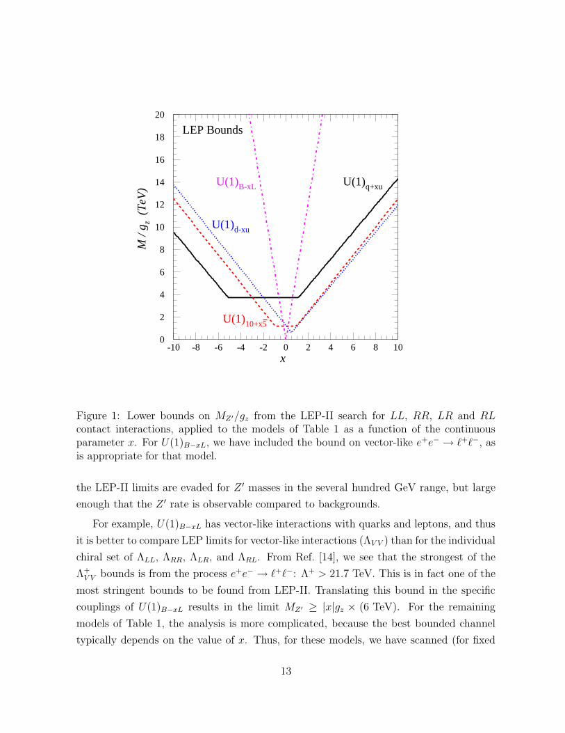
Figure 1: Lower bounds on MZ′/gz from the LEP-II search for LL, RR, LR and RLcontact interactions, applied to the models of Table 1 as a function of the continuousparameter x. For U(1)B−xL, we have included the bound on vector-like e+e− → ℓ+ℓ−, asis appropriate for that model.

the LEP-II limits are evaded for Z ′ masses in the several hundred GeV range, but large

enough that the Z ′ rate is observable compared to backgrounds.

For example, U(1)B−xL has vector-like interactions with quarks and leptons, and thus

it is better to compare LEP limits for vector-like interactions (ΛV V ) than for the individual

chiral set of ΛLL, ΛRR, ΛLR, and ΛRL. From Ref. [14], we see that the strongest of the

Λ+V V bounds is from the process e+e− → ℓ+ℓ−: Λ+ > 21.7 TeV. This is in fact one of the

most stringent bounds to be found from LEP-II. Translating this bound in the specific

couplings of U(1)B−xL results in the limit MZ′ ≥ |x|gz × (6 TeV). For the remaining

models of Table 1, the analysis is more complicated, because the best bounded channel

typically depends on the value of x. Thus, for these models, we have scanned (for fixed

13

−10 ≤ x ≤ 10) through all channels of ΛLL, ΛRR, ΛLR, ΛRL and chosen the best bound.

The results are shown in Figure 1. It is interesting to note that for |x| ∼> 1, U(1)B−xL is

very strongly constrained by LEP II data, whereas for x → 0 the coupling to electrons

becomes small and the bounds disappear.

We have compared our results for general x with the E6-inspired models studied in

detail at LEP-II [14]. As explained above, these correspond to specific points in x for a

given model family. We find that our results agree with the LEP bounds for the dedicated

analysis at or better than the 25% level (depending on the model), thus indicating that

our procedure does a good job in comparison with the dedicated analysis for the points in

which the two may be compared. For most of the parameter space there is no dedicated

LEP analysis, and we present for the first time the LEP bounds on the general class of

Z ′ models.

Generically, the fact that LEP II was an e+e− collider implies that these strong bounds

can be evaded by a Z ′ which couples only very weakly to electrons2. Also, different chiral

structures than the vector-like interactions of U(1)B−xL can have weaker bounds. From

Ref. [14] one observes that a Z ′ which couples only to left-handed or right-handed electrons

is bounded only by Λ+ ≥ 7.1, 7.0 TeV (for ΛLL and ΛRR, respectively). This implies a

bound of MZ′ ≥ gzz × (1.9 TeV), approximately three times weaker than the bound on

U(1)B−xL.

3 Z ′ Searches at the Tevatron

At the Tevatron, searches for additional neutral gauge bosons can be performed in a

variety of processes. If such bosons couple to the SM quarks, they may be directly

observed through their production and subsequent decay into high energy lepton pairs or

jets. The case of the decay into leptons is particularly attractive due to low backgrounds

and good momentum resolution. Bounds on several models containing extra neutral gauge

bosons, have been set by both the CDF [18, 19, 20] and D0 [21, 22, 23] experiments by

measuring high energy lepton pair production cross sections. Searches have been made in

the e+e− channel, which has the best acceptance, and thus best systematics, as well as in

the µ+µ− channel. More recently, the challenging τ+τ− channel has also been analyzed

[24]. The µ+µ− and τ+τ− final states, along with the Z ′ decay into jets which suffers from

2For example, theories such as Top-color assisted Technicolor [15], Top-flavor [16], or SupersymmetricTop-flavor [17], have small couplings to the first generation.

14

huge QCD backgrounds, can probe Z ′ bosons with suppressed couplings to the electrons,

which are not constrained by the LEP searches.

In what follows, we will restrict ourselves to the study of the leptonic decay modes,

proposing a simple, model-independent, parameterization for the Z ′ production cross

section and analyzing its theoretical and experimental feasibilities and limitations.

3.1 Z ′ Hadro-production

The additional terms, beyond those coming from SM particles, in the differential cross

section for production of a pair of charged leptons due to the presence of an extra neutral

gauge boson can be written as [25]

d

dQ2σ(

pp→ Z ′X → l+l−X)

=1

sσ(Z ′ → l+l−)WZ′

(

s,Q2)

+dσintdQ2

, (3.1)

where Q is the invariant mass of the lepton pair, and√s is the energy of the pp collision

in the center-of-momentum frame. The first term accounts for the contributions from

the Z ′ itself and has been explicitly factorized into a hadronic structure function, WZ′,

containing all the QCD dependence and the couplings of quarks to the Z ′, and

σ(Z ′ → l+l−) =g2z

4π

(

z2lj

+ z2ej

288

)

Q2

(Q2 −M2Z′)2 +M2

Z′ Γ2Z′

. (3.2)

Up to NLO in QCD, only the partonic processes qq → Z ′X (non-singlet) and qg → Z ′X

contribute to the hadronic structure function. If the Z ′ couplings to quarks are generation

independent, both processes give contributions which are proportional to (z2q + z2

u) or

(z2q + z2

d) for up and down type quarks, respectively. Therefore, the hadronic structure

function can be written as

WZ′

(

s,M2Z′

)

= g2z

[

(z2q + z2

u)wu(

s,M2Z′

)

+ (z2q + z2

d)wd(

s,M2Z′

)

]

. (3.3)

The functions wu and wd do not depend on any coupling and are exactly the same for

any model containing neutral gauge bosons coupled in a generation independent way to

quarks. In the MS scheme, they are given by

wu(d) =∑

q=u,c(d,s,b)

∫ 1

0

dx1

∫ 1

0

dx2

∫ 1

0

dz{

fq/P (x1,M2Z′) fq/P (x2,M

2Z′) ∆qq(z,M

2Z′)

+ fg/P (x1,M2Z′)[

fq/P (x2,M2Z′) + fq/P (x2,M

2Z′)]

∆gq(z,M2Z′)

+ (x1 ↔ x2, P ↔ P )}

δ

(

M2Z′

s− z x1 x2

)

, (3.4)

15

where fi/P (x,M2) and fi/P (x,M2) are the PDFs for the proton and antiproton, respec-

tively, and

∆qq(z,M2Z′) = δ(1 − z) +

αs(M2Z′)

πCF

[

δ(1 − z)

(

π2

3− 4

)

+ 4

(

ln(1 − z)

1 − z

)

+z[0,1]

− 2 (1 + z) ln(1 − z) − 1 + z2

1 − zln z

]

, (3.5)

∆gq(z,M2Z′) =

αs(M2Z′)

2πTF

[

(

1 − 2z + 2z2)

ln(1 − z)2

z+

1

2+ 3z − 7

2z2

]

. (3.6)

The color factors are CF = 4/3 and TF = 1/2, and we have set the renormalization and

factorization scales to MZ′ .

The second term in Eq. (3.1), dσint/dQ2, corresponds to the interference of the Z ′

with the Z and the photon. If the Z ′ resonance is narrow enough, the interference of the

Z ′ with the Z and photons can be neglected (see the Appendix).

In the narrow width approximation, the expression for the total cross section is simply

obtained from the differential cross section, explicitly

σ(

pp→ Z ′X → l+l−X)

=π

48 sWZ′

(

s,M2Z′

)

Br(Z ′ → l+l−) , (3.7)

where Br(Z ′ → l+l−) is the branching ratio for the decay of Z ′ into the corresponding

pair of leptons. Using the expression of the hadronic structure function, Eq. (3.3), one

obtains

σ(

pp→ Z ′X → l+l−X)

=π

48 s

[

cuwu(

s,M2Z′

)

+ cdwd(

s,M2Z′

)]

. (3.8)

The coefficients cu and cd, given by

cu,d = g2z (z2

q + z2u,d) Br(Z ′ → l+l−) , (3.9)

contain all the dependence on the couplings of quarks and leptons to the Z ′, while wu and

wd only depend on the mass of the gauge boson and can be calculated in a completely

model-independent way.

The parameterization given in Eq. (3.8) permits a direct extraction of a bound in

the cu − cd plane from the experimental limit for the cross section, which can be later

compared to the predictions of particular models. This fact is particularly useful for

models admitting free parameters like the ones discussed in the preceding sections. In

16

10-4

10-3

10-2

10-4

10-3

10-2

10-1

cd

c u

MZ'=600 GeV

MZ'=700 GeV

MZ'=800 GeV B-xL

Figure 2: Excluded regions in the cd − cu plane from the current 95% C.L. limit forσ · Br(Z ′ → l+l−) given in [28], for different values of the Z ′ mass. The thick straightline corresponds to values of cu and cd in the B − xL model, in which cu = cd. The areabetween the two thin straight lines is the region where the q + xu model lies.

particular, these quantities are simply computed for a given Z ′ model, without need to

compute the hadro-production cross section, and thus are a common ground between

theory and experiment.

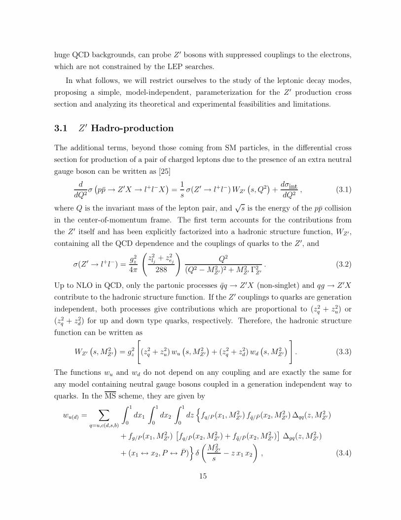
The D0 and CDF Collaborations have set preliminary 95% C.L. limits for σ ·Br(Z ′ →l+l−) in Run II with 200 fb−1 [27, 28]. In Figure 2 we show the excluded regions in the

cd − cu plane for different values of the mass of the Z ′ boson as obtained from the limit

on σ ·Br(Z ′ → l+l−) given by the CDF Collaboration [28] in Run II with 200 fb−1. Very

similar results are obtained using the results by the D0 Collaboration [27]. The wu and

wd coefficients in Eq. (3.8) for this plot were calculated at NLO with MRST02 PDFs [29].

From the current generation of CTEQ [30] PDFs, one obtains very similar results.

It is instructive to compare these limits with the predictions of the four families of

models presented in Section 2. The values of cu and cd as functions of the gauge coupling

gz and the x parameter are given in Table 2 In Figure 2 displays the values of (cd, cu)

corresponding to the B − xL and q + xu models. In the B − xL case, these points are

17

U(1)B−xL U(1)q+xu U(1)10+x5 U(1)d−xu

cu/g2z

4x2

9(4+9x2)

(1+x2)(13+4x+x2)27(40−8x+7x2)

2(1+x2)135(2+x2)

x2(1−2x+2x2)27(5−4x+6x2)

cd/cu 1 1 + 4 1−x1+x2

1+x2

21x2

Table 2: Predictions for cd and cu in four families of models defined in Table 1. Thebranching fractions are computed at tree level for M ′

Z > 2mt and assuming decaysonly into SM particles.

constrained to satisfy cu = cd, corresponding to the thick straight line. For the q + xu

model, the allowed region is

(3 − 2√

2) cd ≤ cu ≤ (3 + 2√

2) cd , (3.10)

which corresponds to the area between the two thin straight lines in Figure 2. The 10+x 5

model, in turn, is constrained to the region cu ≤ 2 cd, whereas there are no constraints for

the possible values of cd and cu in the d− xu model.

3.2 Higher-order corrections

At NNLO in QCD, the general expression in Eq. (3.3) is no longer valid. This is due to

the contributions from the partonic processes qq → Z ′X (singlet) and qq → Z ′X, which

depend upon a variety of coupling combinations in addition to (z2q + z2

u) and (z2q + z2

d).

Thus, one should worry whether cu and cd are a sufficient description of the model. The

actual size of these corrections can be estimated by looking at a particular model. In

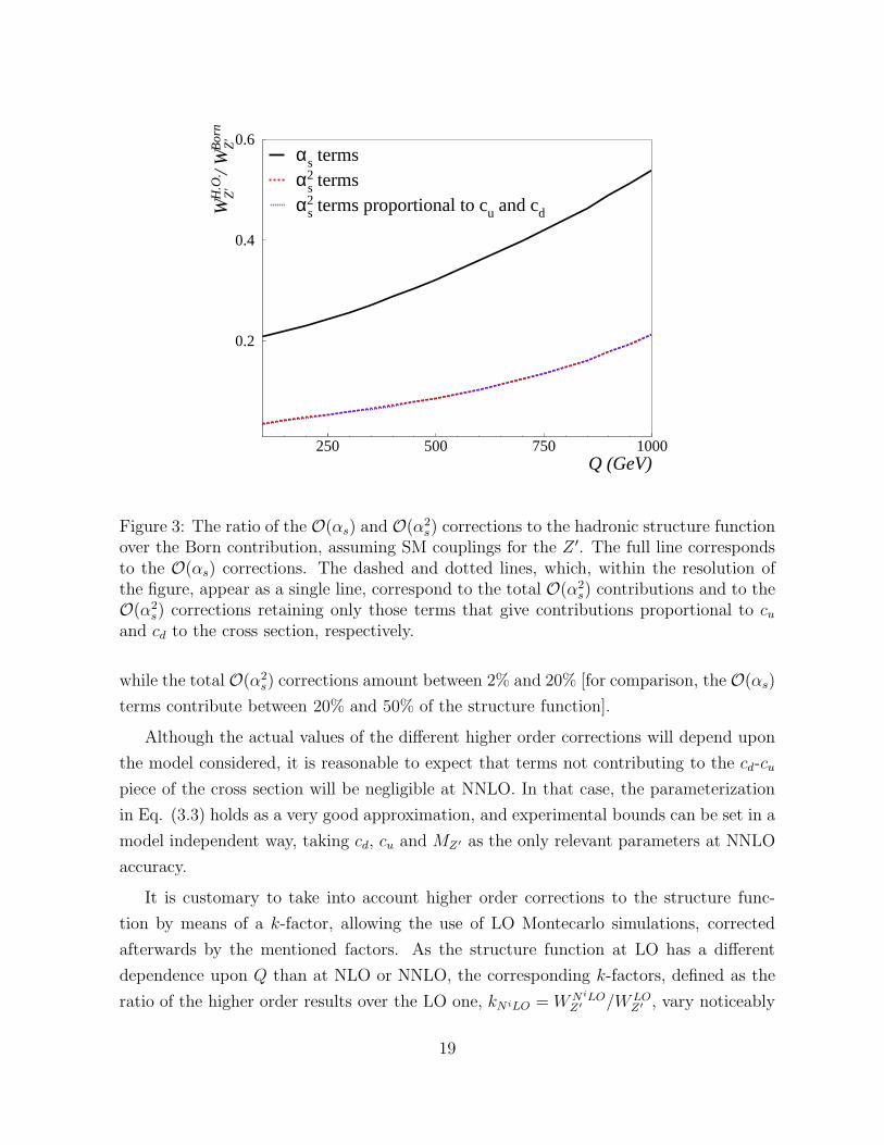
Figure 3 we plot the sizes of the O(αs) and O(α2s) terms to the structure function at

NNLO relative to the Born contribution for the case of SM-like couplings of the Z ′ boson.

The NNLO corrections were calculated with the program ZPROD [25, 26, 31] and the

MRST02 NNLO set of PDFs [29]. We have split the O(α2s) corrections in two parts,

one proportional to cd and cu, and the other depending upon other combinations of the

couplings. Contributions proportional to cd and cu, coming from O(α2s) corrections to

processes already present at lower orders, are clearly the dominant ones, overcoming the

remaining pieces by more than an order of magnitude in the whole Q range. Typically

the terms with mixed couplings contribute less than one per mil to the structure function,

18

Q (GeV)

WZ

' H

.O.

/ W

Z'

Bor

n

αs termsαs

2 termsαs

2 terms proportional to cu and cd

0.2

0.4

0.6

250 500 750 1000

Figure 3: The ratio of the O(αs) and O(α2s) corrections to the hadronic structure function

over the Born contribution, assuming SM couplings for the Z ′. The full line correspondsto the O(αs) corrections. The dashed and dotted lines, which, within the resolution ofthe figure, appear as a single line, correspond to the total O(α2

s) contributions and to theO(α2

s) corrections retaining only those terms that give contributions proportional to cuand cd to the cross section, respectively.

while the total O(α2s) corrections amount between 2% and 20% [for comparison, the O(αs)

terms contribute between 20% and 50% of the structure function].

Although the actual values of the different higher order corrections will depend upon

the model considered, it is reasonable to expect that terms not contributing to the cd-cu

piece of the cross section will be negligible at NNLO. In that case, the parameterization

in Eq. (3.3) holds as a very good approximation, and experimental bounds can be set in a

model independent way, taking cd, cu and MZ′ as the only relevant parameters at NNLO

accuracy.

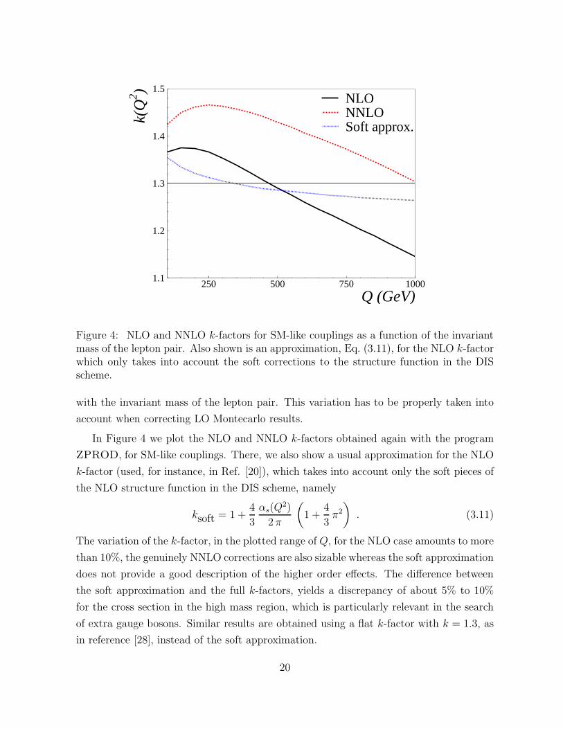
It is customary to take into account higher order corrections to the structure func-

tion by means of a k-factor, allowing the use of LO Montecarlo simulations, corrected

afterwards by the mentioned factors. As the structure function at LO has a different

dependence upon Q than at NLO or NNLO, the corresponding k-factors, defined as the

ratio of the higher order results over the LO one, kN iLO = WN iLOZ′ /WLO

Z′ , vary noticeably

19

Q (GeV)

k(Q

2 )

NLONNLOSoft approx.

1.1

1.2

1.3

1.4

1.5

250 500 750 1000

Figure 4: NLO and NNLO k-factors for SM-like couplings as a function of the invariantmass of the lepton pair. Also shown is an approximation, Eq. (3.11), for the NLO k-factorwhich only takes into account the soft corrections to the structure function in the DISscheme.

with the invariant mass of the lepton pair. This variation has to be properly taken into

account when correcting LO Montecarlo results.

In Figure 4 we plot the NLO and NNLO k-factors obtained again with the program

ZPROD, for SM-like couplings. There, we also show a usual approximation for the NLO

k-factor (used, for instance, in Ref. [20]), which takes into account only the soft pieces of

the NLO structure function in the DIS scheme, namely

ksoft = 1 +4

3

αs(Q2)

2 π

(

1 +4

3π2

)

. (3.11)

The variation of the k-factor, in the plotted range of Q, for the NLO case amounts to more

than 10%, the genuinely NNLO corrections are also sizable whereas the soft approximation

does not provide a good description of the higher order effects. The difference between

the soft approximation and the full k-factors, yields a discrepancy of about 5% to 10%

for the cross section in the high mass region, which is particularly relevant in the search

of extra gauge bosons. Similar results are obtained using a flat k-factor with k = 1.3, as

in reference [28], instead of the soft approximation.

20

So far we only discussed QCD corrections to the Z ′ cross section, which are of the

order of 30% as can be seen from the k-factors in Figure 4. There are also corrections from

the electroweak sector, which we will address briefly. The complete O(α) corrections to

the SM contributions to neutral current Drell-Yan process were calculated in [32]. There,

it was found that these corrections are large, particularly in the high invariant mass

region, being of the order of 12% at Tevatron energies for mll ≃ 700 GeV in the electron

channel. Besides affecting the background for the search of additional neutral gauge

bosons, electroweak radiative corrections also modify the signal cross section. However,

as we will see, these effects are substantially smaller for the Z ′ terms.

As shown in [32], the main contributions to the electroweak corrections come from the

box diagrams and cannot be factorized into effective couplings and masses. In particular,

box diagrams with two charged bosons give rise to large double logarithms which are

the origin of the large corrections in the high mass region. On the other hand, box

diagrams that include neutral bosons (γ, Z0 and Z ′) always appear in combination with

their crossed versions and that leads to a cancellation of the double logs [33]. Then, the

non-factorizable contributions that affect exclusively the signal cross section only include

subleading simple logs and thus the corrections are expected to be smaller than for the

SM background.

The remaining contributions come from QED and factorizable purely weak corrections.

The later can always be absorbed into effective couplings and masses, thus, they do not

affect the signal cross section where these quantities are treated as free parameters. The

main electromagnetic contributions come from large logarithms due to collinear photon

emission in the initial and final states, and affect both the signal and background cross

sections. The large contributions coming from initial state radiation can be factorized

into the PDFs, modifying the DGLAP evolution equations for the partonic densities.

After factorization, the remaining terms are typically at the per mil level, reaching 1% in

the high momentum fraction region [32] whereas the QED modifications to the evolution

equations are small and neglected in comparison to the uncertainties in the PDFs [34].

However, collinear emission in the final state gives corrections of the order of 5% for the

electron channel in the high mass region, and a careful analysis should probably take

them into account.

21

3.3 Model dependence in experimental bounds

As we have shown in the previous section, the parametrization given in Eq. (3.8) allows to

extract model independent constraints on the coefficients cd and cu from the experimental

results for the lepton pair production cross section. A key assumption for this analysis is

that the bounds for the cross section can be extracted from data in a model independent

manner. In particular, the experimental analyses involve corrections for the finite accep-

tance of the detectors to extract the total cross section. As the acceptance is obtained

from detailed Monte Carlo simulations, which need to assume particular values of the

couplings, it is far from trivial that this procedure does not introduce model dependence

into the experimental bounds.

In Ref. [18], the changes in the acceptance with variations in the couplings of up and

down quarks were studied. There, it was found that the acceptance changes very little

when considering the limiting cases of either decoupling up or down quarks. However,

this study was limited to SM-like couplings for electrons, a feature that, a priori, might be

too restrictive. To study the actual model dependence of the experimental acceptance, in

this section, we will consider the angular distribution of the lepton pair and apply simple

cuts on this distribution. For simplicity we will restrict to the LO approximation.

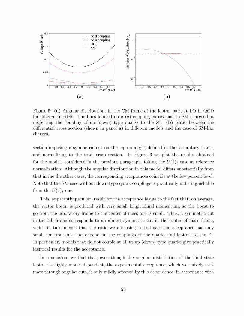
In the left panel of Figure 5 we plot the LO cross section differential with respect to the

azimuthal angle, in the center of mass frame of the lepton pair, with different assumptions

for the couplings, setting MZ′ = 600 GeV. We considered SM-like couplings, SM-like

couplings with up or down couplings neglected and the E6 inspired model U(1)I mentioned

in Section 2. The right panel shows the ratios between the cross section in the last three

cases to the cross section with SM couplings. Except for the overall normalization, the

cases where the Z ′ does not couple to either up or down type quarks differ very little from

the SM case. This feature can be traced back to the peculiar fact that, in the SM, the

left and right handed couplings of charged leptons, satisfy z2l − z2

e = sin2 θW −1/4 ≃ 0.02.

Then, the terms odd under θ → −θ are suppressed relative to the even ones in the LO

differential cross section, which turns out to be nearly symmetric. This characteristic

feature is in sharp contrast with the behavior in the U(1)I case, where the asymmetry

is almost maximal. This is related to the vanishing of the couplings of the right-handed

electrons and left-handed down-type quarks to the Z ′ in this last model.

To get a handle on how the noticeable differences in the angular distribution affect

the experimental acceptance, we crudely estimated it by integrating the differential cross

22

cos θ* (CM)

dσ/d

cos

θ* (pb

)

no d couplingno u couplingU(1)ΙSM

0

0.05

0.1

0.15

0.2

-1 -0.8 -0.6 -0.4 -0.2 0 0.2 0.4 0.6 0.8 1

(a)

cos θ* (CM)

(dσ/

dcos

θ* )/

(dσ/

dcos

θ* ) SM

10-2

10-1

1

-1 -0.8 -0.6 -0.4 -0.2 0 0.2 0.4 0.6 0.8 1

(b)

Figure 5: (a) Angular distribution, in the CM frame of the lepton pair, at LO in QCDfor different models. The lines labeled no u (d) coupling correspond to SM charges butneglecting the coupling of up (down) type quarks to the Z ′. (b) Ratio between thedifferential cross section (shown in panel a) in different models and the case of SM-likecharges.

section imposing a symmetric cut on the lepton angle, defined in the laboratory frame,

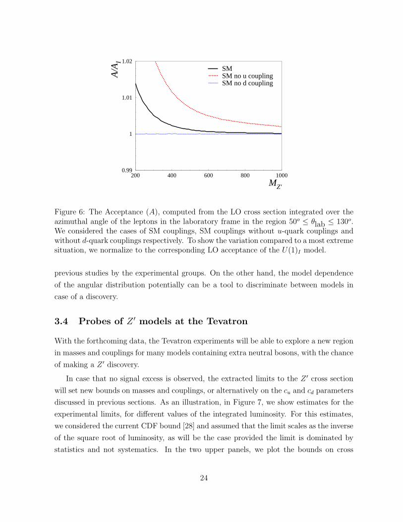
and normalizing to the total cross section. In Figure 6 we plot the results obtained

for the models considered in the previous paragraph, taking the U(1)I case as reference

normalization. Although the angular distribution in this model differs substantially from

that in the the other cases, the corresponding acceptances coincide at the few percent level.

Note that the SM case without down-type quark couplings is practically indistinguishable

from the U(1)I one.

This, apparently peculiar, result for the acceptance is due to the fact that, on average,

the vector boson is produced with very small longitudinal momentum, so the boost to

go from the laboratory frame to the center of mass one is small. Thus, a symmetric cut

in the lab frame corresponds to an almost symmetric cut in the center of mass frame,

which in turn means that the ratio we are using to estimate the acceptance has only

small contributions that depend on the couplings of the quarks and leptons to the Z ′.

In particular, models that do not couple at all to up (down) type quarks give practically

identical results for the acceptance.

In conclusion, we find that, even though the angular distribution of the final state

leptons is highly model dependent, the experimental acceptance, which we naively esti-

mate through angular cuts, is only mildly affected by this dependence, in accordance with

23

MZ'

A/A

I

SMSM no u couplingSM no d coupling

0.99

1

1.01

1.02

200 400 600 800 1000

Figure 6: The Acceptance (A), computed from the LO cross section integrated over theazimuthal angle of the leptons in the laboratory frame in the region 50o ≤ θlab ≤ 130o.We considered the cases of SM couplings, SM couplings without u-quark couplings andwithout d-quark couplings respectively. To show the variation compared to a most extremesituation, we normalize to the corresponding LO acceptance of the U(1)I model.

previous studies by the experimental groups. On the other hand, the model dependence

of the angular distribution potentially can be a tool to discriminate between models in

case of a discovery.

3.4 Probes of Z ′ models at the Tevatron

With the forthcoming data, the Tevatron experiments will be able to explore a new region

in masses and couplings for many models containing extra neutral bosons, with the chance

of making a Z ′ discovery.

In case that no signal excess is observed, the extracted limits to the Z ′ cross section

will set new bounds on masses and couplings, or alternatively on the cu and cd parameters

discussed in previous sections. As an illustration, in Figure 7, we show estimates for the

experimental limits, for different values of the integrated luminosity. For this estimates,

we considered the current CDF bound [28] and assumed that the limit scales as the inverse

of the square root of luminosity, as will be the case provided the limit is dominated by

statistics and not systematics. In the two upper panels, we plot the bounds on cross

24

gZ’=0.1

Z’ mass (GeV)

σ B

r(Z

’→ee

) (p

b) B-xL

x=1/3

x=1

x=3

200 pb-1

2 fb-1

10 fb-1

10-3

10-2

10-1

1

200 400 600 800

gZ’=0.1

Z’ mass (GeV)

σ B

r(Z

’→ee

) (p

b) 10+x5−

x=0

x=3

x=6

200 pb-1

2 fb-1

10 fb-1

10-3

10-2

10-1

1

200 400 600 800

10-4

10-3

10-2

10-4

10-3

10-2

10-1

cd

c u

MZ'=600 GeV MZ'=700 GeV MZ'=800 GeV

2 fb-1

B-xL

a

b

c

Figure 7: Projected bounds for the B − xL (left upper panel) and 10 + x5 (right upperpanel) models and projected excluded regions in the cd−cu plane (lower panel). In the twoupper panels, the vertical marks show the current LEP bounds for the Z ′ mass obtained asdescribed in Section 2.3. In the B−xL case, for x = 3 this last bound is MZ′ ≥ 1800 GeV;for the 10 + x5, the bound for x = 0 is MZ′ ≥ 119 GeV, beyond the scope of the figure.The projected bounds at luminosities L = 2 fb−1 , 10 fb−1 are obtained from Fig. 2 byscaling with a factor 1/

√L. The lower panel also shows the regions in the cd − cu plane

corresponding to the B − xL and q + xu models, as in Figure 2, showing the projectedincrease in reach with 2 fb−1. The dots labeled a, b and c correspond to the B−L modelwith gz = 0.1, gz = 0.3 and gz = 0.5, respectively.

section times branching ratio, as a function of MZ′ , together with the predictions for

different values of x in the B− xL (left) and in the 10 + x5 (right) models. We also show

25

the mass bounds, for the different cases, set by the LEP contact interaction constraints

discussed before. The lower panel shows the excluded regions in the cd − cu plane for

different values of the Z ′ mass, assuming an integrated luminosity of 2 fb−1.

The results in Figure 7 show that, both in the cases of the B−xL and 10+x5 models,

there is a sizable unexplored region in parameter space that the Tevatron will certainly

be able to probe. For the B − xL models, LEP bounds are stronger for larger values of

|x|, while the Tevatron can do much better for |x| ∼< 1. For the 10+x5 models, the LEP

bounds are slightly weaker than in the previous case and the unbounded region in x space

is larger.

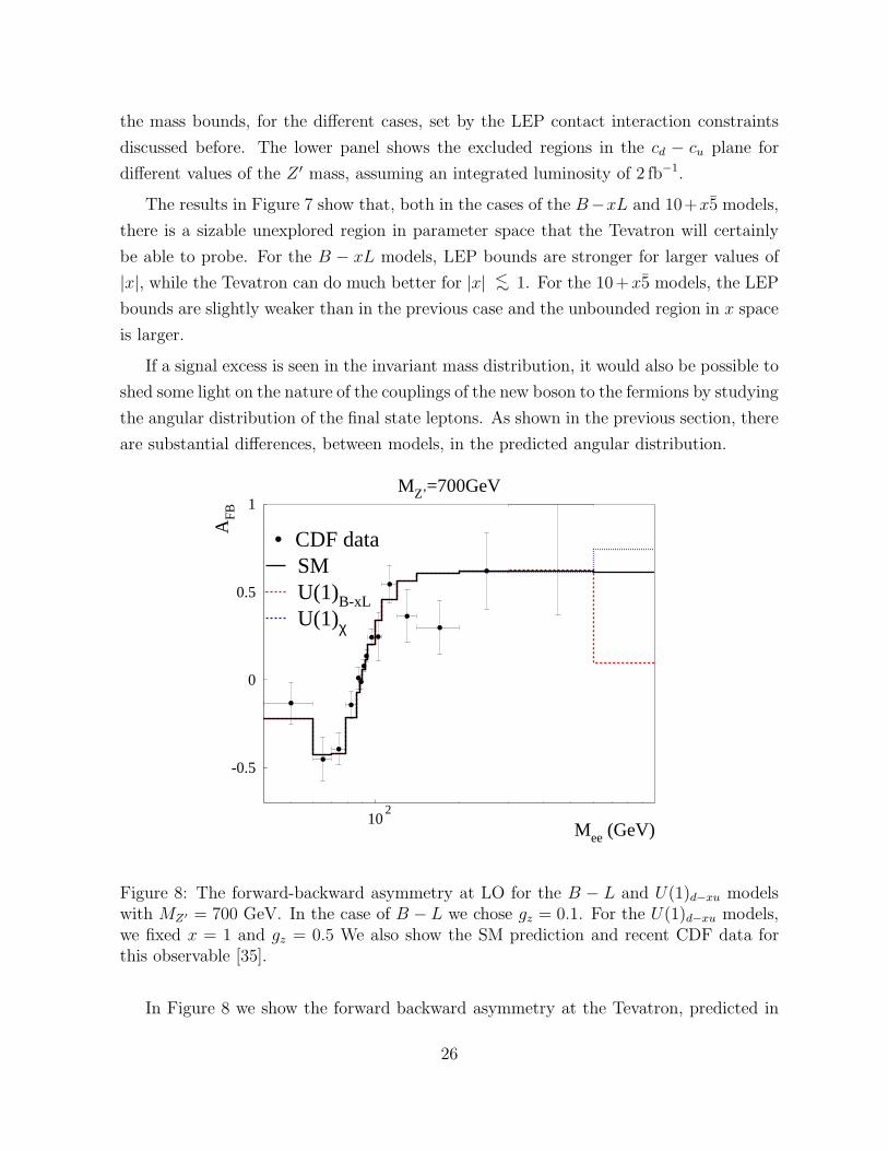
If a signal excess is seen in the invariant mass distribution, it would also be possible to

shed some light on the nature of the couplings of the new boson to the fermions by studying

the angular distribution of the final state leptons. As shown in the previous section, there

are substantial differences, between models, in the predicted angular distribution.

-0.5

0

0.5

1

102

MZ’=700GeV

Mee (GeV)

AFB

CDF dataSMU(1)B-xLU(1)χ

Figure 8: The forward-backward asymmetry at LO for the B − L and U(1)d−xu modelswith MZ′ = 700 GeV. In the case of B − L we chose gz = 0.1. For the U(1)d−xu models,we fixed x = 1 and gz = 0.5 We also show the SM prediction and recent CDF data forthis observable [35].

In Figure 8 we show the forward backward asymmetry at the Tevatron, predicted in

26

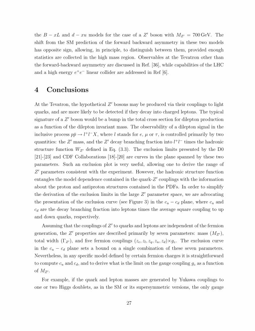
the B − xL and d − xu models for the case of a Z ′ boson with MZ′ = 700 GeV. The

shift from the SM prediction of the forward backward asymmetry in these two models

has opposite sign, allowing, in principle, to distinguish between them, provided enough

statistics are collected in the high mass region. Observables at the Tevatron other than

the forward-backward asymmetry are discussed in Ref. [36], while capabilities of the LHC

and a high energy e+e− linear collider are addressed in Ref [6].

4 Conclusions

At the Tevatron, the hypothetical Z ′ bosons may be produced via their couplings to light

quarks, and are more likely to be detected if they decay into charged leptons. The typical

signature of a Z ′ boson would be a bump in the total cross section for dilepton production

as a function of the dilepton invariant mass. The observability of a dilepton signal in the

inclusive process pp→ l+l−X, where l stands for e, µ or τ , is controlled primarily by two

quantities: the Z ′ mass, and the Z ′ decay branching fraction into l+l− times the hadronic

structure function WZ′ defined in Eq. (3.3). The exclusion limits presented by the D0

[21]-[23] and CDF Collaborations [18]-[20] are curves in the plane spanned by these two

parameters. Such an exclusion plot is very useful, allowing one to derive the range of

Z ′ parameters consistent with the experiment. However, the hadronic structure function

entangles the model dependence contained in the quark-Z ′ couplings with the information

about the proton and antiproton structures contained in the PDFs. In order to simplify

the derivation of the exclusion limits in the large Z ′ parameter space, we are advocating

the presentation of the exclusion curve (see Figure 3) in the cu − cd plane, where cu and

cd are the decay branching fraction into leptons times the average square coupling to up

and down quarks, respectively.

Assuming that the couplings of Z ′ to quarks and leptons are independent of the fermion

generation, the Z ′ properties are described primarily by seven parameters: mass (MZ′),

total width (ΓZ′), and five fermion couplings (ze, zl, zq, zu, zd)×gz. The exclusion curve

in the cu − cd plane sets a bound on a single combination of these seven parameters.

Nevertheless, in any specific model defined by certain fermion charges it is straightforward

to compute cu and cd, and to derive what is the limit on the gauge coupling gz as a function

of MZ′.

For example, if the quark and lepton masses are generated by Yukawa couplings to

one or two Higgs doublets, as in the SM or its supersymmetric versions, the only gauge

27

groups that may provide a Z ′ gauge boson accessible at the Tevatron are of the type

U(1)B−xL. This means that all fermion charges are determined by a single parameter, x.

Within this family of gauge groups, cu and cd have a simple dependence on x and gz; for

a given x and MZ′ , the limit on gz can be immediately derived.

If the quark and lepton masses are generated by a more general mechanism, Z ′ gauge

bosons associated with gauge groups other than U(1)B−xL may be accessible at the Teva-

tron. We have presented three other examples of one-parameter families of U(1) gauge

groups, chosen to include (for particular values of the parameter x) many of the Z ′ models

discussed in the literature. For these families of models, the Tevatron reach goes signif-

icantly beyond the LEP II bounds for large regions of the three dimensional parameter

space spanned by MZ′, gz and x.

Relaxing the assumption that the couplings of Z ′ to leptons are generation inde-

pendent, for each of the e+e−, µ+µ− and τ+τ− final states there is a different cu and

cd. Interestingly, U(1) gauge groups that lead to a Z ′ of this type exist even when the

anomalies cancel without need for new fermions charged under the SM group, and the

quark and lepton masses are generated by Yukawa couplings to a single Higgs doublet.

Such Z ′ bosons may have very small couplings to electrons, evading altogether the LEP

bounds, and could be discovered in the µ+µ− or τ+τ− channels at the Tevatron.

Although generation-independent Z ′ couplings to quarks are tightly constrained by

measurements of various flavor-changing neutral currents, a Z ′ with different couplings to

the d and s quarks (or to the u and c quarks) in the mass range accessible at the Tevatron

cannot be completely ruled out. In that case, the cu and cd parameterization would have

to be supplemented by cs (or cc, cb) quantities. Even in this case, the fact that current-

and next-generation hadron colliders collide nucleons (and anti-nucleons) implies that cu

and cd typically remain the most important, because of their large valence distribution

functions (particularly at large parton x) for nucleons.

Observables other than the total cross section for dilepton production can also be

measured at the Tevatron. We have discussed the additional information provided by

the forward-backward asymmetry. In most cases however, a Z ′ discovery is more likely

to occur first as a bump in the dilepton total cross section. If that happens, MZ′ can

be determined by the invariant mass of the lepton pair, and a curve (actually a band of

experimental error bars) in the cu − cd plane can be derived. For each Z ′ model (fixed

x within the one-parameter families), the curve would determine the gauge coupling.

However, pinning down the model would be difficult, requiring additional observables at

28

the Tevatron and future colliders.

Acknowledgements:

The authors have benefitted from discussions with Ayres Freitas and Beate Heine-

mann. A.D. thanks the Theory Department at Fermilab for their warm hospitality and

financial support, and CONICET, Argentina, for financial support. Fermilab is operated

by Universities Research Association Inc. under contract no. DE-AC02-76CH02000 with

the DOE.

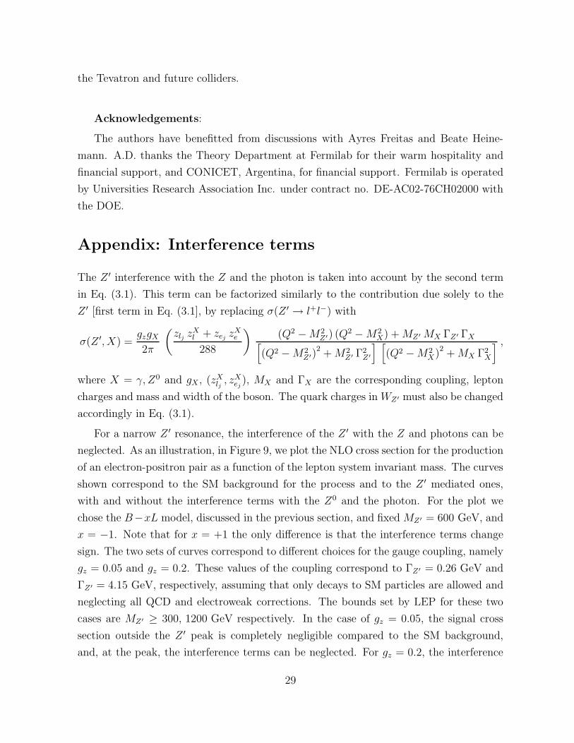
Appendix: Interference terms

The Z ′ interference with the Z and the photon is taken into account by the second term

in Eq. (3.1). This term can be factorized similarly to the contribution due solely to the

Z ′ [first term in Eq. (3.1], by replacing σ(Z ′ → l+l−) with

σ(Z ′, X) =gzgX2π

(

zlj zXl + zej

zXe288

)

(Q2 −M2Z′) (Q2 −M2

X) +MZ′ MX ΓZ′ ΓX[

(Q2 −M2Z′)

2+M2

Z′ Γ2Z′

] [

(Q2 −M2X)

2+MX Γ2

X

] ,

where X = γ, Z0 and gX , (zXlj , zXej

), MX and ΓX are the corresponding coupling, lepton

charges and mass and width of the boson. The quark charges in WZ′ must also be changed

accordingly in Eq. (3.1).

For a narrow Z ′ resonance, the interference of the Z ′ with the Z and photons can be

neglected. As an illustration, in Figure 9, we plot the NLO cross section for the production

of an electron-positron pair as a function of the lepton system invariant mass. The curves

shown correspond to the SM background for the process and to the Z ′ mediated ones,

with and without the interference terms with the Z0 and the photon. For the plot we

chose the B−xL model, discussed in the previous section, and fixed MZ′ = 600 GeV, and

x = −1. Note that for x = +1 the only difference is that the interference terms change

sign. The two sets of curves correspond to different choices for the gauge coupling, namely

gz = 0.05 and gz = 0.2. These values of the coupling correspond to ΓZ′ = 0.26 GeV and

ΓZ′ = 4.15 GeV, respectively, assuming that only decays to SM particles are allowed and

neglecting all QCD and electroweak corrections. The bounds set by LEP for these two

cases are MZ′ ≥ 300, 1200 GeV respectively. In the case of gz = 0.05, the signal cross

section outside the Z ′ peak is completely negligible compared to the SM background,

and, at the peak, the interference terms can be neglected. For gz = 0.2, the interference

29

Z'→ e+e- (MZ'=600GeV, gz=0.05)

Mll (GeV)

dσ/d

M (

pb/G

eV)

Total cross sectionNo interferenceSM background

10-6

10-5

10-4

10-3

10-2

400 500 600 700 800

(a)

Z'→ e+e- (MZ'=600GeV, gz=0.2)

Mll (GeV)

dσ/d

M (

pb/G

eV)

10-6

10-5

10-4

10-3

10-2

400 500 600 700 800

(b)

Figure 9: NLO differential cross sections for the production of electron-positron pairs asa function of the invariant mass of the pair, in the U(1)B+L model. The solid curvescorrespond to the total cross sections for the signal, including interference terms, for thegauge coupling fixed to gz = 0.05 and gz = 0.2 respectively. Dashed lines are the samecross sections neglecting interference terms and the dotted lines correspond to the SMbackground.

terms are more important and contribute to the tails at low and high mass. However, the

experimental errors would not allow one to disentangle the signal from the background

outside the peak, where again, the signal cross section is dominated by terms containing

only Z ′ propagators.

References

[1] E. Eichten, I. Hinchliffe, K. D. Lane and C. Quigg, “Super Collider Physics,” Rev.

Mod. Phys. 56, 579 (1984) [Addendum-ibid. 58, 1065 (1986)].

[2] For a review, see J. L. Hewett and T. G. Rizzo, “Low-Energy Phenomenology Of

Superstring Inspired E(6) Models,” Phys. Rept. 183, 193 (1989);

[3] See, e.g., M. Cvetic and P. Langacker, “Implications of Abelian Extended

Gauge Structures From String Models,” Phys. Rev. D 54, 3570 (1996)

[arXiv:hep-ph/9511378].

30

[4] For a review, see A. Leike, “The phenomenology of extra neutral gauge bosons,”

Phys. Rept. 317, 143 (1999) [arXiv:hep-ph/9805494].

[5] T. Appelquist, B. A. Dobrescu and A. R. Hopper, “Nonexotic neutral gauge bosons,”

Phys. Rev. D 68, 035012 (2003) [arXiv:hep-ph/0212073].

[6] A. Freitas, “Weakly coupled neutral gauge bosons at future linear colliders,”

arXiv:hep-ph/0403288.

[7] For a recent review, see, G. Altarelli and M. W. Grunewald, “Precision electroweak

tests of the standard model,” arXiv:hep-ph/0404165.

[8] P. Abreu et al. [DELPHI Collaboration], Z. Phys. C 65, 603 (1995).

[9] M. S. Chanowitz, “The Z → anti-b b decay asymmetry: Lose-lose for the

standard model,” Phys. Rev. Lett. 87, 231802 (2001) [arXiv:hep-ph/0104024];

M. S. Chanowitz, “Electroweak data and the Higgs boson mass: A case for new

physics,” Phys. Rev. D 66, 073002 (2002) [arXiv:hep-ph/0207123]; D. Choudhury,

T. M. P. Tait and C. E. M. Wagner, “Beautiful mirrors and precision electroweak

data,” Phys. Rev. D 65, 053002 (2002) [arXiv:hep-ph/0109097].

[10] J. Erler and P. Langacker, “Indications for an extra neutral gauge boson in elec-

troweak precision data,” Phys. Rev. Lett. 84, 212 (2000) [arXiv:hep-ph/9910315];

P. Langacker and M. Plumacher, “Flavor changing effects in theories with a heavy

Z’ boson with family non-universal couplings,” Phys. Rev. D 62, 013006 (2000)

[arXiv:hep-ph/0001204].

[11] M. Carena, T. M. P. Tait and C. E. M. Wagner, “Branes and orbifolds are opaque,”

Acta Phys. Polon. B 33, 2355 (2002) [arXiv:hep-ph/0207056].

[12] For example, N. Arkani-Hamed, A. G. Cohen, E. Katz and A. E. Nelson, “The littlest

Higgs,” JHEP 0207, 034 (2002) [arXiv:hep-ph/0206021].

[13] C. Csaki, J. Hubisz, G. D. Kribs, P. Meade and J. Terning, “Big corrections from a

little Higgs,” Phys. Rev. D 67, 115002 (2003) [arXiv:hep-ph/0211124]; J. L. Hewett,

F. J. Petriello and T. G. Rizzo, “Constraining the littlest Higgs. ((U)),” JHEP 0310,

062 (2003) [arXiv:hep-ph/0211218].

[14] [LEP Collaboration], “A combination of preliminary electroweak measurements and

constraints on the standard model,” arXiv:hep-ex/0312023.

31

[15] C. T. Hill, “Topcolor assisted technicolor,” Phys. Lett. B 345, 483 (1995)

[arXiv:hep-ph/9411426]; R. S. Chivukula and E. H. Simmons, “Electroweak limits on

non-universal Z’ bosons,” Phys. Rev. D 66, 015006 (2002) [arXiv:hep-ph/0205064].

[16] R. S. Chivukula, E. H. Simmons and J. Terning, “Limits on noncommuting extended

technicolor,” Phys. Rev. D 53, 5258 (1996) [arXiv:hep-ph/9506427]; D. J. Muller

and S. Nandi, “Topflavor: A Separate SU(2) for the Third Family,” Phys. Lett. B

383, 345 (1996) [arXiv:hep-ph/9602390]; E. Malkawi, T. Tait and C. P. Yuan, “A

Model of Strong Flavor Dynamics for the Top Quark,” Phys. Lett. B 385, 304 (1996)

[arXiv:hep-ph/9603349]; H. J. He, T. Tait and C. P. Yuan, “New topflavor models

with seesaw mechanism,” Phys. Rev. D 62, 011702 (2000) [arXiv:hep-ph/9911266].

[17] P. Batra, A. Delgado, D. E. Kaplan and T. M. P. Tait, “The Higgs mass bound in

gauge extensions of the minimal supersymmetric standard model,” JHEP 0402, 043

(2004) [arXiv:hep-ph/0309149]; P. Batra, A. Delgado, D. E. Kaplan and T. M. P. Tait,

“Running into new territory in SUSY parameter space,” arXiv:hep-ph/0404251.

[18] F. Abe et al. [CDF Collaboration], “A Search for new gauge bosons in anti-p p

collisions at S**(1/2) = 1.8-TeV,” Phys. Rev. Lett. 68, 1463 (1992).

[19] F. Abe et al. [CDF Collaboration], “Search for new gauge bosons decaying into

dielectrons in anti-p p collisions at s**(1/2) 1.8-TeV,” Phys. Rev. D 51, 949 (1995).

[20] F. Abe et al. [CDF Collaboration], “Search for new gauge bosons decaying into

dileptons in anti-p p collisions at s**(1/2) = 1.8-TeV,” Phys. Rev. Lett. 79, 2192

(1997).

[21] S. Abachi et al. [D0 Collaboration], “Search for additional neutral gauge bosons,”

Phys. Lett. B 385, 471 (1996).

[22] B. Abbott et al. [D0 Collaboration], “Measurement of the high-mass Drell-Yan cross

section and limits on quark-electron compositeness scales,” Phys. Rev. Lett. 82, 4769

(1999) [arXiv:hep-ex/9812010].

[23] V. M. Abazov et al. [D0 Collaboration], “Search for heavy particles decaying into

electron positron pairs in p anti-p collisions,” Phys. Rev. Lett. 87, 061802 (2001)

[arXiv:hep-ex/0102048].

32

[24] Talk at Fermilab by Anton Anastassov, July 23, 2004,

http://theory.fnal.gov/jetp/previous.html.

[25] R. Hamberg, W. L. van Neerven and T. Matsuura, “A Complete Calculation Of The

Order Alpha-S**2 Correction To The Drell-Yan K Factor,” Nucl. Phys. B 359, 343

(1991) [Erratum-ibid. B 644, 403 (2002)].

[26] R. V. Harlander and W. B. Kilgore, “Next-to-next-to-leading order Higgs production

at hadron colliders,” Phys. Rev. Lett. 88, 201801 (2002) [arXiv:hep-ph/0201206].

[27] D0 Collaboration, note 4375-Conf, “Search for heavy Z’ Bosons in the Dielectron

Channel with 200 pb−1 of Data.”

[28] Tracey Pratt (for the CDF Collaboration), talk at the SUSY 2004 Conference, June

2004.

[29] A. D. Martin, R. G. Roberts, W. J. Stirling and R. S. Thorne, “NNLO global parton

analysis,” Phys. Lett. B 531, 216 (2002) [arXiv:hep-ph/0201127].

[30] J. Pumplin, D. R. Stump, J. Huston, H. L. Lai, P. Nadolsky and W. K. Tung, JHEP

0207, 012 (2002) [arXiv:hep-ph/0201195].

[31] http://www.lorentz.leidenuniv.nl∼neerven/

[32] U. Baur, O. Brein, W. Hollik, C. Schappacher and D. Wackeroth, “Electroweak ra-

diative corrections to neutral-current Drell-Yan processes at hadron colliders,” Phys.

Rev. D 65, 033007 (2002) [arXiv:hep-ph/0108274].

[33] P. Ciafaloni and D. Comelli, “Sudakov effects in electroweak corrections,” Phys. Lett.

B 446, 278 (1999) [arXiv:hep-ph/9809321].

[34] U. Baur, S. Keller and W. K. Sakumoto, “QED radiative corrections to Z

boson production and the forward backward Phys. Rev. D 57, 199 (1998)

[arXiv:hep-ph/9707301].

[35] Data extracted from the plots in http://www-cdf.fnal.gov/physics/ewk/2004/afb/

[36] S. Ambrosanio et al. [MSSM Working Group Collaboration], “Report of the Beyond

the MSSM subgroup for the Tevatron Run II SUSY / Higgs workshop,” Sec. XV

arXiv:hep-ph/0006162.

33