Embed Size (px)
Citation preview

C.B. Wang
Application of Integrable Systems to Phase Transitions

Application of Integrable Systems to PhaseTransitions

C.B. Wang
Application ofIntegrable Systemsto Phase Transitions

C.B. WangInstitute of AnalysisTroy, USA
ISBN 978-3-642-38564-3 ISBN 978-3-642-38565-0 (eBook)DOI 10.1007/978-3-642-38565-0Springer Heidelberg New York Dordrecht London
Library of Congress Control Number: 2013945531
Mathematics Subject Classification: 82B26, 82B27, 81V22, 81V05, 81V15, 34M03, 33C45, 34M55,35Q15, 34E05, 34F10, 91B80
© Springer-Verlag Berlin Heidelberg 2013This work is subject to copyright. All rights are reserved by the Publisher, whether the whole or part ofthe material is concerned, specifically the rights of translation, reprinting, reuse of illustrations, recitation,broadcasting, reproduction on microfilms or in any other physical way, and transmission or informationstorage and retrieval, electronic adaptation, computer software, or by similar or dissimilar methodologynow known or hereafter developed. Exempted from this legal reservation are brief excerpts in connectionwith reviews or scholarly analysis or material supplied specifically for the purpose of being enteredand executed on a computer system, for exclusive use by the purchaser of the work. Duplication ofthis publication or parts thereof is permitted only under the provisions of the Copyright Law of thePublisher’s location, in its current version, and permission for use must always be obtained from Springer.Permissions for use may be obtained through RightsLink at the Copyright Clearance Center. Violationsare liable to prosecution under the respective Copyright Law.The use of general descriptive names, registered names, trademarks, service marks, etc. in this publicationdoes not imply, even in the absence of a specific statement, that such names are exempt from the relevantprotective laws and regulations and therefore free for general use.While the advice and information in this book are believed to be true and accurate at the date of pub-lication, neither the authors nor the editors nor the publisher can accept any legal responsibility for anyerrors or omissions that may be made. The publisher makes no warranty, express or implied, with respectto the material contained herein.
Printed on acid-free paper
Springer is part of Springer Science+Business Media (www.springer.com)

This book is dedicated to my parents, my wifeLing Shen and my lovely children Shela andHenry.

Preface
This book is aimed at providing a unified eigenvalue density formulation of matrixmodels and discussing the corresponding phase transitions and critical phenomena.The purpose of this book is to systematically classify the transition models based onthe potential functions that define the consequent integrable systems, string equa-tions, eigenvalue densities, free energies and critical points considered in the transi-tions.
The unification of different couplings or interactions is one of the important re-search topics in quantum chromodynamics (QCD) theory that can help to studythe dominance of confinement or asymptotic freedom in low or high energy scale.Hilbert space theory and Fourier analysis are the necessary mathematical tools towork on the physical problems. As a foundation of the Hilbert space theory, orthog-onal polynomials can provide a new mathematical background for further investi-gating the fundamental concepts such as position and momentum described in theHeisenberg uncertainty principle that is tightly related to matrix models which areimportant in QCD.
In quantum physics the probability amplitude for a particle to travel from onepoint to another in a given time is characterized by propagator. By the Fourier trans-form, the propagator becomes a singular function in the momentum space, where thesingularity is related to the uncertainty. Correlation function in the matrix modelscan avoid such singularity in large-N asymptotics that leads the eigenvalue densityto represent the momentum so that free energy function can be properly formulated.String equation is a tool in the momentum aspect to construct the eigenvalue densi-ties and give parameter relations in the models for finding the phase transitions. Theassociated integrable systems imply a unified formula for the different densities inthe matrix models by using the Lax pair structures obtained from the correspondingorthogonal polynomials.
Analytic results derived from the integrable systems will reduce the mathematicalcomplexity in discussing the phase transition problems of the matrix models. Thedifferent density phases can be generated from the scalings of the string equationand associated discrete differential equations in the Lax pair with proper periodicreductions implemented by using an index folding technique in large-N scaling.
vii

viii Preface
The different scalings can have a common case which is the critical point separatingtwo phases with different conditions. The string equation properly establishes thenonlinear relations between the parameters in the model such that behaviors of thefree energy around the critical point can be easily obtained, either analytically or bythe expansions according to the parameter relations. The first-, second- and third–order transition models can be created by using the string equation, Toda latticeand corresponding integrable systems. Expansions for the coupling parameters inassociation with the double scalings present a new strategy to find the divergencetransitions or critical phenomena with a fractional power-law.
Phase transition models discussed by using the string equations differ from thetransitions in traditional models such as the Ising models, but there is a similaritybetween the periodic reduction that reorganizes wave functions in the momentumaspect using the index folding and the idea of renormalization in statistical mechan-ics that reorganizes the particles in the position aspect. Typically, the critical pointin the bifurcation transition is when the center or radius parameter is bifurcated,while the critical point in the renormalization method is a fixed point in an iterationprocess. The power-law at the critical point in the momentum aspect is derived fromthe algebraic equation reduced from the string equation that is the parameter con-dition(s) different from the renormalization groups considered in the Ising models.In addition, eigenvalue density on multiple disjoint intervals and corresponding freeenergy can be referred to study Seiberg-Witten differential and prepotential in theSeiberg-Witten theory which is developed to solve the mass gap problem in quantumYang-Mills theory.
The organization of this book is as follows. Chapter 1 is about the physical back-ground of the matrix models. The unified model proposed in this book is fundamen-tal for the phase transitions. Chapter 2 is for the reduction of eigenvalue densitiesfrom the integrable systems. In Chaps. 3 and 4, various transitions will be discussedfor the Hermitian matrix models. In Chaps. 5 and 6, we will talk about the transitionsand critical phenomena in the unitary matrix models, including the Gross-Wittenthird-order phase transition. Chapter 7 deals with the Marcenko-Pastur distribution,McKay’s law and their generalizations in association with the Laguerre and Jacobipolynomials.
This book is about how to find the phase transitions, which can be used as a refer-ence book for researchers and students in the fields of phase transitions and criticalphenomena in quantum physics. I thank Professor J. Bryce McLeod for his direc-tions and help on both the related works in this book and previous works. I thankCraig A. Tracy for introducing the random matrix theory, and thank Gunduz Cagi-nalp, Xinfu Chen, Palle Jorgensen, Juan Manfredi and William Troy for the usefuldiscussions or suggestions. And I thank Xing-biao Hu, Zaijiu Shang and LianwenZhang for the helpful discussions and encouragement.
Chie Bing WangTroy, USAApril 2012

Contents
1 Introduction . . . . . . . . . . . . . . . . . . . . . . . . . . . . . . . . 11.1 Unified Model for the Eigenvalue Densities . . . . . . . . . . . . . 11.2 String Equation and Matrix Models . . . . . . . . . . . . . . . . . 51.3 Critical Point in Gross-Witten Model . . . . . . . . . . . . . . . . 101.4 Phase Transitions in the Momentum Aspect . . . . . . . . . . . . . 13References . . . . . . . . . . . . . . . . . . . . . . . . . . . . . . . . . 18
2 Densities in Hermitian Matrix Models . . . . . . . . . . . . . . . . . 212.1 Generalized Hermite Polynomials . . . . . . . . . . . . . . . . . . 212.2 Integrable System and String Equation . . . . . . . . . . . . . . . 252.3 Factorization and Asymptotics . . . . . . . . . . . . . . . . . . . 302.4 Density Models . . . . . . . . . . . . . . . . . . . . . . . . . . . 372.5 Special Densities . . . . . . . . . . . . . . . . . . . . . . . . . . . 42References . . . . . . . . . . . . . . . . . . . . . . . . . . . . . . . . . 44
3 Bifurcation Transitions and Expansions . . . . . . . . . . . . . . . . 453.1 Free Energy for the One-Interval Case . . . . . . . . . . . . . . . 453.2 Partition Function and Toda Lattice . . . . . . . . . . . . . . . . . 523.3 Merged and Split Densities . . . . . . . . . . . . . . . . . . . . . 553.4 Third-Order Phase Transition by the ε-Expansion . . . . . . . . . 593.5 Symmetric Cases . . . . . . . . . . . . . . . . . . . . . . . . . . . 68References . . . . . . . . . . . . . . . . . . . . . . . . . . . . . . . . . 73
4 Large-N Transitions and Critical Phenomena . . . . . . . . . . . . . 754.1 Cubic Potential . . . . . . . . . . . . . . . . . . . . . . . . . . . . 75
4.1.1 Models in Large-N Asymptotics . . . . . . . . . . . . . . 754.1.2 First-Order Discontinuity . . . . . . . . . . . . . . . . . . 784.1.3 Fifth-Order Phase Transition . . . . . . . . . . . . . . . . 83
4.2 Quartic Potential . . . . . . . . . . . . . . . . . . . . . . . . . . . 864.2.1 Second-Order Transition . . . . . . . . . . . . . . . . . . . 874.2.2 Critical Phenomenon . . . . . . . . . . . . . . . . . . . . 88
4.3 General Quartic Potential . . . . . . . . . . . . . . . . . . . . . . 91
ix
x Contents
4.3.1 Density Model with Discrete Parameter . . . . . . . . . . . 914.3.2 Expansion for the Generalized Model . . . . . . . . . . . . 944.3.3 Double Scaling at the Critical Point . . . . . . . . . . . . . 98
4.4 Searching for Fourth-Order Discontinuity . . . . . . . . . . . . . . 101References . . . . . . . . . . . . . . . . . . . . . . . . . . . . . . . . . 105
5 Densities in Unitary Matrix Models . . . . . . . . . . . . . . . . . . . 1075.1 Variational Equation . . . . . . . . . . . . . . . . . . . . . . . . . 1075.2 Recursion and Discrete AKNS-ZS System . . . . . . . . . . . . . 1105.3 Lax Pair and String Equation . . . . . . . . . . . . . . . . . . . . 113
5.3.1 Special Potential . . . . . . . . . . . . . . . . . . . . . . . 1135.3.2 General Potential . . . . . . . . . . . . . . . . . . . . . . 120
5.4 Densities Reduced from the Lax Pair . . . . . . . . . . . . . . . . 1245.4.1 Strong Couplings: General Case . . . . . . . . . . . . . . . 1265.4.2 Weak Couplings: One-Cut Cases . . . . . . . . . . . . . . 1265.4.3 Weak Coupling: Two-Cut Case . . . . . . . . . . . . . . . 1275.4.4 Weak Coupling: Three-Cut Case . . . . . . . . . . . . . . 129
References . . . . . . . . . . . . . . . . . . . . . . . . . . . . . . . . . 130
6 Transitions in the Unitary Matrix Models . . . . . . . . . . . . . . . 1316.1 Large-N Models and Partition Function . . . . . . . . . . . . . . . 1316.2 First-Order Discontinuity with Two Cuts . . . . . . . . . . . . . . 1356.3 Double Scaling Associated with Gross-Witten Transition . . . . . 1406.4 Third-Order Transitions for the Multi-cut Cases . . . . . . . . . . 1486.5 Divergences for the One-Cut Cases . . . . . . . . . . . . . . . . . 154References . . . . . . . . . . . . . . . . . . . . . . . . . . . . . . . . . 158
7 Marcenko-Pastur Distribution and McKay’s Law . . . . . . . . . . . 1617.1 Laguerre Polynomials and Densities . . . . . . . . . . . . . . . . 1617.2 Divergences Related to Marcenko-Pastur Distribution . . . . . . . 1677.3 Jacobi Polynomials and Logarithmic Divergences . . . . . . . . . 1767.4 Integral Transforms for the Density Functions . . . . . . . . . . . 183References . . . . . . . . . . . . . . . . . . . . . . . . . . . . . . . . . 187
Appendix A Some Integral Formulas . . . . . . . . . . . . . . . . . . . . 191
Appendix B Properties of the Elliptic Integrals . . . . . . . . . . . . . . 195B.1 Asymptotics of the Elliptic Integrals . . . . . . . . . . . . . . . . 195B.2 Elliptic Integrals Associated with Legendre’s Relation . . . . . . . 197
Appendix C Lax Pairs Based on the Potentials . . . . . . . . . . . . . . 203C.1 Cubic Potential . . . . . . . . . . . . . . . . . . . . . . . . . . . . 203C.2 Quartic Potential . . . . . . . . . . . . . . . . . . . . . . . . . . . 205C.3 Potential in the Unitary Model . . . . . . . . . . . . . . . . . . . . 206
Appendix D Hypergeometric-Type Differential Equations . . . . . . . . 211D.1 Singular Points in the Hermitian Model . . . . . . . . . . . . . . . 211D.2 Singular Points in the Unitary Model . . . . . . . . . . . . . . . . 213
Index . . . . . . . . . . . . . . . . . . . . . . . . . . . . . . . . . . . . . . 217

Chapter 1Introduction
Phase transition problems in the one-matrix models in QCD are discussed in thisbook by using string equations. The phase transition models are formulated by usingeigenvalue density which represents the momentum operator described in quantummechanics. By using orthogonal polynomials, the eigenvalue densities in variousmatrix models can be unified. The string equation establishes a connection betweenthe position and momentum aspects described in the Heisenberg uncertainty prin-ciple, which is important and usually hard to find in other methods. The recursionformula of the orthogonal polynomials can be applied to introduce an index foldingtechnique to reorganize the wave functions in order to achieve a renormalization inthe momentum aspect. It will be discussed that the critical phenomenon associatedwith the Gross-Witten model can be found by using Toda lattice and double scaling.The hypergeometric-type differential equations improve on some shortages of inte-grable systems to work on physical problems, such as the fact that a soliton systemdoes not have a differential equation along the spectrum direction, and illustrate anew background to study the singularities of physical quantities, such as mass.
1.1 Unified Model for the Eigenvalue Densities
The well known Wigner semicircle [59, 60] was found in 1955 to represent theenergy spectrum distributed on the real line, and now it has been applied as a fun-damental eigenvalue density model in many scientific areas. Distribution shapes ofthe eigenvalues reflect a scientific character of the natural phenomena that have mo-tivated scientists to find further density models to reveal new sciences. And manynew discoveries have been made, including the Marcenko-Pastur distribution [36]and McKay’s law [37] found in the research of random matrices and random graphsin 1967 and 1981, respectively. These models have been widely applied in quantumphysics and complexity research in recent years in order to find the natural rules be-hind the random phenomena. In this book, we are going to discuss that orthogonalpolynomials can be applied to derive these important models and introduce a uni-fied model for these different density models that further confirms the significance
C.B. Wang, Application of Integrable Systems to Phase Transitions,DOI 10.1007/978-3-642-38565-0_1, © Springer-Verlag Berlin Heidelberg 2013
1
2 1 Introduction
of eigenvalue densities in the quantum models and complexity sciences. The methodcan be generalized to get various density models, including the phase models in thephase transition problems. Let us first use some samples to see how these modelsare related to orthogonal polynomials.
Consider the Hermite polynomials Hn(z) satisfying∫∞−∞Hm(z)Hn(z)e
−V (z)dz= 2nn!√πδm,n, where V (z) = z2. In some literatures, V (x) is called external po-tential. In this book, we will simply call it potential or potential function. Letpn(z) = Hn(z)/2n = zn + · · · , and Φn(z) = e−V (z)/2(pn(z),pn−1(z))
T . By thederivative formula of the Hermite polynomials from the textbook, it can be veri-fied that Φn(z) satisfies an equation d
dzΦn =An(z)Φn, where
An(z)=(−z n
−2 z
)
, (1.1)
and trAn(z)= 0. Let z= √nη. Then
1
nπ
√detAn(z)dz= 1
π
√2 − η2dη, (1.2)
with |η| ≤ √2, which gives the Wigner semicircle density [59, 60] for the rescaled
potential W(η) = η2. It should be noted that the semicircle is introduced here justfor the basic density concept. The Wigner semicircle model that has been widelyconsidered in the random researches such as random matrix theory, does not have aphase transition. The phase transitions or critical phenomena discussed in this bookare all for the generalized models from the basic models presented in this section.
If the potential is changed to V (z)= tz2, then
An(z)=(−tz 2tvn
−2t tz
)
, (1.3)
where vn satisfies
2tvn = n. (1.4)
This trivial algebraic equation is a simple string equation. Complicated string equa-tions will appear when the potential V (x) is changed to a higher degree polynomial.In the following samples, there will be similar string equations if the potential ischanged by adding some parameter(s) like the t above. Now, let us just show howorthogonal polynomials can be applied to provide a unified structure to constructdifferent fundamental density models.
The next sample is the Marcenko-Pastur distribution. Consider the Laguerrepolynomials L(α)n (z) satisfying
∫∞0 L
(α)m (z)L
(α)n (z)zαe−zdz= Γ (α + 1)
(n+αn
)δm,n,
where α > −1, and Γ (·) is the Gamma function. For the Laguerre polynomials,choose Φn(z) = zα/2e−z/2(L
(α)n (z),L
(α)n−1(z))
T . By using the differential equation
for the Laguerre polynomials, we have that Φn(z) satisfies an equation ddzΦn =

1.1 Unified Model for the Eigenvalue Densities 3
An(z)Φn, where
An(z)= 1
z
(− z−α2 + n −n− α
n z−α2 − n
)
, (1.5)
and trAn(z)= 0. Let z= nη, q = nn+α , η+ = (1 + 1√
q)2 and η− = (1 − 1√
q)2. Then
there is [39]
1
(n+ α)π
√detAn(z)dz= q
2πη
√(η+ − η)(η− η−)dη, (1.6)
with η− ≤ η ≤ η+, which gives the Marcenko-Pastur distribution [36]. This densityfunction is also discussed in [51], and it has been popularly applied in econophysicsto study the distribution of the positive eigenvalues.
Another fundamental model, McKay’s law [37], is associated with the Jacobipolynomials P (α,β)
n (z) satisfying∫ 1−1P
(α,β)m (z)P
(α,β)n (z)w(z)dz = hnδmn, defined
on the interval [−1,1] with the weight w(z)= (1 − z)α(1 + z)β , where α >−1 andβ > −1. Let Φn(z) = w(z)1/2(P
(α,β)n (z),P
(α,β)
n−1 (z))T . If we choose β = α, then
Φn(z) satisfies an equation ddzΦn =An(z)Φn, where
An(z)= 1
1 − z2
(−(n+ α)z n+ α
−n(n+2α)n+α (n+ α)z
)
, (1.7)
obtained by using the differential equation of the Jacobi polynomials. Let z = η/c
and α/n= c/2 − 1, then we get
1
nπ
√detAn(z)dz= c
2π(c2 − η2)
√4(c− 1)− η2dη, (1.8)
with |η| ≤ 2√c− 1 and c > 1, where the density function on the right hand side
above is called McKay’s law, see [37].Now, let us consider the simple orthogonal polynomials pn(z) = zn on the unit
circle z= eiθ in the complex plane, satisfying∮pm(z)pn(z)
dz2πiz = δm,n, where the
integral is over the unit circle |z| = 1, and pn(z)= z−n is the complex conjugate ofpn(z). It can be shown that Φn(z)= (z−n/2pn(z), z
n/2pn(z))T satisfies an equation
ddzΦn =An(z)Φn, where
An(z)=( n
2z 00 − n
2z
)
. (1.9)
The weight is equal to 1, the potential is U(z)= 0, and pn(0)= 0. It is easy to seethat
1
nπ
√detAn(z)dz= 1
2πdθ, −π ≤ θ ≤ π. (1.10)
The right hand side is a uniform distribution, which is a degenerate case of theGross-Witten strong coupling density model in the unitary matrix model [22] when

4 1 Introduction
the temperature is equal to infinity. The Gross-Witten weak and strong couplingdensity models can be obtained by changing the potential to U(z)= s(z+ z−1), andthe weight for the orthogonality is then changed to exp(s(z + z−1)) implying thefollowing generalized coefficient matrix [39]
An(z)=(
s2 + s
2z2 + n−2sxnxn+12z s(xn+1 − xn
z)z−1
s(xn − xn+1z) − s
2 − s
2z2 − n−2sxnxn+12z
)
, (1.11)
where xn = pn(0) ∈ [0,1] satisfying another string equation,
s(1 − x2
n
)xn+1 + xn−1
−xn = n. (1.12)
The phase transitions considered in QCD are about the change from one densitymodel to another one. So the density models in the matrix model theory in QCDare no longer as simple as we have seen above, but multiple reductions from thecoefficient matrix An. It will be discussed in detail in Chaps. 5 and 6 that if xn+1 ∼−xn ∼ xn−1, then T = n/s = 2(1 − x2
n)(≤ 2), and
1
nπ
√detAn(z)dz∼ 2
πTcos
θ
2
√T
2− sin2 θ
2dθ, (1.13)
where z= eiθ . If T > 2, then xn → 0, and
1
nπ
√detAn(z)dz∼ 1
2π
(
1 + 2
Tcos θ
)
dθ. (1.14)
These are the weak and strong coupling eigenvalue densities in the Gross-Wittenthird-order phase transition model [22], which is the fundamental reference for thetransition models discussed in this book.
We have seen that the eigenvalue densities, which will be denoted by ρ in laterdiscussions, can always be obtained from the unified model
1
nπ
√detAn(z), (1.15)
where the matrix An is derived from the orthogonal polynomials. The idea of theabove unified density model was first introduced in [39]. We use the terminology“unified model” here as a guidance for the readers to see how the densities will beconstructed in this book. By this unified model of the eigenvalue densities, we canstudy relations between the different states or couplings of the physical model. Phasetransition is one of the theories to find the critical point with discontinuous propertyof the free energy in order to separate different states. This book is planned to studya type of phase transition models based on the unified model and string equations. InChap. 2, we will use generalized Hermite polynomials to get many density modelsto extend the Wigner semicircle that will be applied to study transition problems inChaps. 3 and 4 for the Hermitian matrix models.

1.2 String Equation and Matrix Models 5
The orthogonality is a typical case of consistency considered in integrable sys-tems. Orthogonal polynomials provide an easy method to find integrable systemfor string equations or Toda lattice, which is then a generalization of orthogonalpolynomial system. In an integrable system, the parameters are allowed to vary ina wider space than in orthogonal polynomial system. For example, for the potentialV (x)= tx2 discussed above, the parameter t needs to be positive in the orthogonalpolynomials. While in integrable system, t can be negative. Such extensions alsoapply to other potentials. In phase transition models, the parameters can be any-where in the space with complicated nonlinear relations that are generally very hardto figure out in other methods. The analysis based on string equations naturally fol-lows the orthogonality or consistency structure to get nonlinear relations and avoidssolving complicated equations that traditional methods often depend on.
When the eigenvalue density problems are solved, elliptic integrals in the freeenergy function are the next consideration for the phase transition problems, whichare generally not easy. We will use contour integrals, asymptotics, initial valueproblems, recursive relations, hypergeometric differential equations and Legendre’srelation to discuss the elliptic integrals. However, these methods are not enoughto always solve behaviors of the free energy function at the critical point. Theε-expansion method for the parameter equations obtained from the string equationsand associated large-N double scaling method are necessary techniques to derive thediscontinuity or divergence in transition, and it works for all the transition problemsto be discussed in this book.
1.2 String Equation and Matrix Models
Now let us generalize the weight function e−z2of the Hermite polynomials to a new
weight function e−V (z) where V (z)= tz2 + z4, and consider orthogonal polynomi-als pn(z) = zn + · · · satisfying
∫∞−∞ pm(z)pn(z)e
−(tz2+z4)dz = hnδmn. The quan-tity Zn,
Zn = n!h0h1 · · ·hn−1, (1.16)
called partition function, is a function of t and n. This formula holds when V (z) ischanged to a general potential, and it will be used to define free energy in the tran-sition problem. The orthogonal polynomials can be applied to get the derivative(s)of the logarithm of the partition function, lnZn. It will be discussed in Sect. 3.2 thatthe derivatives of hn and vn = hn/hn−1 have simple formulations, and the partitionfunction will be proved to satisfy the following relation,
d2
dt2lnZn = vn(vn−1 + vn+1), (1.17)
for n≥ 2. The first-order derivative has a complicated formula than the second orderderivative (1.17), that will be explained in Sect. 3.2. These formulas are based onderivative formula of the vn, called Toda lattice.

6 1 Introduction
The parameters or functions in the orthogonal polynomials need to be rescaledto study the physical problems in the matrix models. Specially, lnZn needs to berescaled to get the free energy function, and then all the corresponding relationsneed to be rescaled consequently. The questions include which equations need to beinvolved and how to implement the rescaling. For the phase transition problems inour consideration, we need a string equation in the Hermitian matrix model,
2tvn + 4(vn+1 + vn + vn−1)vn = n, (1.18)
(called discrete Painlevé I equation in [16]) obtained by Fokas, Its and Kitaev [16] in1991 by using the orthogonality and recursion formula zpn = pn+1 + vnpn−1 [56],which is a three-term recursion formula by counting how many different indexesin the formula. This discrete equation will be related to the parameter condition inthe planar diagram model, which is important for studying the free energy function.The string equation can be reduced to continuum integrable equation in large-Nasymptotics to study the 2D quantum gravity problems, for example, see [6, 11,12, 16, 20]. The phase transition problems discussed in this book will only involvediscrete or continuum equations, not the solutions, to solve the nonlinear relationsof parameters, that are part of the mathematical difficulties in the matrix models. Itis believed that the survey of QCD usually does not start from perturbation analysisor analytical methods, but more likely from lattice gauge theories or matrix modelsas explained in the following.
In 1978, Brezin, Itzykson, Parisi and Zuber [7] introduced the planar diagramtheory to approximate the field theory in order to ultimately provide a mean ofperforming reliable computation in the large coupling phase of non-Abelian gaugefields in four dimensions. The theory is based on the work of ’t Hooft that the onlydiagrams which survive the large-N limit of an SU(N) gauge theory are planar. Theplanar ideas work for Yang-Mills field and other more general fields. The method isto introduce a N × N matrix M = (Mij ) such that the Lagrangian is represented interms of M . Hermitian matrix model is the case when M is a Hermitian matrix asstudied in the planar diagram theory. Free energy E is led to the following relation,
e−n2E(g) = limn→∞
∫exp
{
−1
2trM2 − g
ntrM4
}
dM, (1.19)
where g is the coupling parameter, and
dM =∏
i
dMii
∏
i<j
d(ReMij )d(ImMij ). (1.20)
Because of the complexity of the formulations as seen above, it is developed to studythe partition function
Zn =∫ ∞
−∞· · ·∫ ∞
−∞e−Σn
i=1V (zi )Δ2ndz1 · · ·dzn, (1.21)
1.2 String Equation and Matrix Models 7
where V (z) = t2z2 + t4z
4 and Δn =∏j<k(zj − zk), which is in the scope of non-perturbative theory. The polynomial pn(z) has a representation [56]
pn(z)= Z−1n
∫ ∞
−∞· · ·∫ ∞
−∞e−Σn
i=1V (zi )Δ2n
n∏
j=1
(z− zj )dz1 · · ·dzn, (1.22)
and the orthogonality tells that hn = ∫∞−∞ p2
n(z)e−V (z)dz = ∫∞
−∞ pn(z)zne−V (z)dz.
For Zn+1, we have n+ 1 opportunities to select one of z1, . . . , zn+1 to do the fol-lowing, and each one is equivalent to the operation for zn+1 = z,
Zn+1
n+ 1=∫ ∞−∞
(∫ ∞−∞
· · ·∫ ∞−∞
e−Σni=1V (zi )Δ2
n
n∏
i=1
(z− zi)dz1 · · ·dzn(zn + · · · )
)
e−V (z)dz
=∫ ∞−∞
Znpn(z)(zn + · · · )e−V (z)dz=Znhn,
where “· · · ” in “zn + · · · ” means lower order terms, and Z1 = h0. This has shownthe equation (1.16) for the partition function, which is a basic property in this re-search field. The steepest descent method is used in [7] to study the free energyE = − limn→∞ 1
n2 lnZn in the following way,
E = limn→∞
1
n2
{∑
j
(1
2z2j + g
nz4j
)
−∑
j =kln |zj − zk|
}
, (1.23)
where t2/n = 1/2 and t4 = g, with the stationary condition 12zj + 2 g
nz3j =
∑k =j 1
zj−zk , which can be further scaled to a variational equation
1
2η+ 2gη3 = (P)
∫ 2b
−2b
ρ(λ)
η− λdλ, (1.24)
where ρ(η) = dxdη
is the density of eigenvalues satisfying∫ 2b−2b ρ(η)dη = 1, x is
introduced in η(x) during the scaling zj = √nη(j/n), [−2b,2b] is the interval
where eigenvalues are distributed in, and (P) stands for the principle value of theintegral. The free energy then becomes
E =∫ 2b
−2b
(1
2η2 + gη4
)
ρ(η)dη−∫ 2b
−2b
∫ 2b
−2bln |λ− η|ρ(η)ρ(λ)dλdη. (1.25)
The density ρ(η) above is called planar diagram eigenvalue density model with thefollowing explicit formula [7]
ρ(η)= 1
π
(1
2+ 4gb2 + 2gη2
)√4b2 − η2, (1.26)

8 1 Introduction
for η ∈ [−2b,2b], where
b2 + 12gb4 = 1. (1.27)
The free energy function then has the following explicit formula
E(g)=E(0)+ 1
24
(b2 − 1
)(9 − b2)− 1
2lnb2. (1.28)
It can be calculated that E(0) = 3/4. And E has a singular point at g = gc wheregc = −1/48. In next chapter, we will discuss that the eigenvalue density ρ abovecan be obtained from the unified model 1
nπ
√detA(z) for a generalized matrix An(z)
from (1.3).Since the free energy is obtained in large-N scaling from lnZn, there should be
some relations between the formulas before the scaling and after. If we compare thestring equation (1.18) with (1.27), it can be found that these two algebraic equa-tions have the same nonlinear structure except the coefficients t and g, that can bechanged to be consistent if we consider the general potential V (z) = t2z
2 + t4z4,
and the parameter n can be removed by scaling. This idea inspires us to find a con-nection between the conditions of the parameters in the eigenvalue density and thestring equations. It is found [39] that the string equation properly matches with therestriction conditions for the parameters to solve the stationary condition or varia-tional equation in the Hermitian matrix models, that will be discussed in detail innext chapter.
The method here using string equations to get parameter conditions for the den-sity of eigenvalues differs from the double scaling method in the matrix modelsdeveloped in early 90’s in last century. The early double scaling mainly deals thelimit at a singular point about how a discrete equation can be scaled to a continuumintegrable equation. The previous scaling is in some sense to transform to anotheraspect by the double scaling, whereas the string equation method discussed in thisbook keeps the problem in the same aspect. Interested readers can refer or com-pare the discussions, for example, in [6, 12, 20] for the Hermitian matrix modelsabout the double scaling limit by using the orthogonal polynomials on the real line,as well as in [46–48] for the unitary matrix models which will be discussed in thenext section. The planar diagram model has been generalized to study the regular-ization [31] and phase transition [52] problems. Bleher and Eynard [4] studied athird-order transition model in the Hermitian matrix model in association with theorthogonal polynomials. The double scaling limit of eigenvalue correlations at thecritical points studied in [4] is related to Painlevé II equation, universal kernel and anonlinear hierarchy of ordinary differential equations. The Lax pair method [39] forthe eigenvalue densities in the Hermitian matrix models is to find the mathematicalformulation of the density models and the associated parameter relations by usingstring equation. The string equation provides an much easier method to formulatethe eigenvalue densities than other methods such as loop equations discussed insome literatures. The parameter relations so obtained are the necessary formulas tostudy the phase transition problems that can be seen in later discussions.

1.2 String Equation and Matrix Models 9
The planar diagram model discussed above is a typical Hermitian one-matrixmodel, and there are also multiple matrix models, such as two-matrix model [27, 41]by considering the integral over two matrices,
Zn =∫
exp
{
− tr(M2
1 +M22
)− g
ntr(M4
1 +M42
)+2c tr(M1M2)
}
dM1dM2. (1.29)
The two-matrix model is believed to describe all of (p, q) conformal minimal mod-els in quantum physics, whereas the one-matrix model is for (p,2) minimal models.The partition function given above can be simplified to Zn = const · n!Πn−1
j=0hj by
using the orthogonal polynomials pj (x)= xj +· · · defined by the bi-orthogonality,
∫ ∞
−∞
∫ ∞
−∞pj (x)pk(y) exp
{
−(x2 + y2)− g
n
(x4 + y4)+ 2cxy
}
dxdy = hj δjk.
(1.30)The orthogonal polynomials now satisfy a four-term recursion formula xpj (x) =pj+1 + Rjpj−1(x) + Tjpj−3(x), in which there are four different indexes j + 1,j , j − 1 and j − 3. Discussions for the eigenvalue distribution problems for thetwo-matrix models can be found, for example, in [19, 27, 32, 43], including thedistribution with a gap for constructing the coupling models. The four-term re-cursion formula for the bi-orthogonal polynomials is important in the two-matrixmodels for creating density model with gap(s) according to the literatures. Thedifferential equations [41] and τ -function theory have been applied to study par-tition function in two-matrix model. Bertola [2] computed second- and third-orderderivatives of the free energy in planar limit for arbitrary genus spectral curves us-ing τ -function theory and Bergman kernel which is a bi-differential form, and themethod in principle allows to compute the derivatives of any order. In 2009, Bertolaand Marchal [3] proved that the partition function in the Itzykson-Zuber-Eynard-Mehta two-matrix model is an isomonodromic τ -function as a generalization of theJimbo-Miwa-Ueno’s τ -function [28]. Correlation function and large-N expansionare also researched for the two-matrix models in association with the Yang-Baxterequation [14, 15]. Bethe ansatz for the correlation functions discussed in [15] aboutthe cyclic property is interesting. We will explain later that the cyclic or periodicbehaviors are important for the transition problems.
Split densities with gap(s) in the one-matrix models discussed in this book areobtained by three-term recursion formula of orthogonal polynomials using the indexfolding technique. The three-term recursion formula can be applied to itself to derivesufficient terms for constructing the eigenvalue density on multiple disjoint intervalsto be explained in Sect. 1.4 with concrete recursion formula. Different recursiverelations can be derived depending how to apply the recursion to itself, and thendifferent phases in the transition problems can be constructed, including the densitymodels with gap(s). In this sense, the three-term recursion formula can achieve asimilar role as expected on the four-term recursion formula. Three-term recursionhas a wide application background. The three-term recursion formula is a discreteversion of the Schrödinger equation, which is fundamental in the soliton integrable
10 1 Introduction
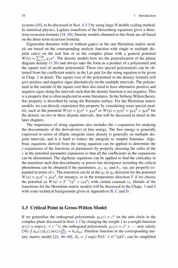
systems [45], to be discussed in Sect. 4.3.3 by using large-N double scaling method.In statistical physics, Laplace transform of the Heisenberg equations gives a three-term recursion formula [34, 50]. Density models obtained in this book are all basedon the three-term recursion formula.
Eigenvalue densities with or without gap(s) in the one Hermitian matrix mod-els are based on the corresponding analytic function with single or multiple dis-joint cut(s) on the real line or in the complex plane with a general potentialW(η) =∑2m
j=1 gjηj . The density models here are the generalization of the planar
diagram density (1.26) and always take the form as a product of a polynomial andthe square root of another polynomial. These two special polynomials can be ob-tained from the coefficient matrix in the Lax pair for the string equation to be givenin Chap. 2 in detail. The square root of the polynomial in the density formula willgive positive and negative signs alternatively on the multiple intervals. The polyno-mial in the outside of the square root then also need to have alternative positive andnegative signs along the intervals such that the density function is not negative. Thisis a property that is often neglected in some literatures. In the Seiberg-Witten theory,this property is described by using the Riemann surface. For the Hermitian matrixmodels, we can directly experience this property by considering some special mod-els, such as the potential W(η)= g2η
2 + g4η4 or W(η)= g2η
2 + g4η4 + g6η
6 forthe density on two or three disjoint intervals, that will be discussed in detail in thelater chapters.
The importance of string equations also includes the ε-expansion for studyingthe discontinuity of the derivative(s) of free energy. The free energy is generallyexpressed in terms of elliptic integrals since density is generally on multiple dis-joint intervals, and it is hard to reduce the integrals to simpler formulas. Alge-braic equations derived from the string equation can be applied to determine theε-expansions of the functions or parameters by properly choosing the order of theε in the potential parameter expansion so that all the coefficients in the expansionscan be determined. The algebraic equations can be applied to find the criticality inthe transition such that discontinuity or power-law divergence including the criticalphenomena can be obtained if the parameters, gj , aj and bj , say, are properly ex-panded in terms of ε. The transition can be in the g2 or g4 direction for the potentialW(η) = g2η
2 + g4η4, for instance, or in the temperature direction T if we choose
the potential as W(η) = T −1(η2 + c0η4) with certain constant c0. Details of the
transitions for the Hermitian matrix models will be discussed in the Chaps. 3 and 4with some technical backgrounds given in Appendices B, C and D.
1.3 Critical Point in Gross-Witten Model
If we generalize the orthogonal polynomials pn(z) = zn on the unit circle in thecomplex plane discussed in Sect. 1.1 by changing the weight 1 to a weight functionw(z)= exp(s(z+ z−1)), the orthogonal polynomials pn(z)= zn + · · · now satisfy[56]
∮pm(z)pn(z)w(z)
dz2πiz = hnδmn. Partition function in the corresponding uni-
tary matrix model [22, 46–48], Zn = ∫ exp{s Tr(U + U†)}dU , can be simplified

1.3 Critical Point in Gross-Witten Model 11
to
Zn = n!h0h1 · · ·hn−1,
similar to the Hermitian matrix model discussed in last section, where U is aN × N unitary matrix and dU is similar to the dM discussed in last section, see[22]. Recursion formula for the polynomials now becomes [38] z(pn + vnpn−1)=pn+1 +unpn, derived from the Szegö’s equation [56]. By orthogonality of the poly-nomials, xn = pn(0, s) satisfy a different string equation [38, 46, 47, 58]
n
sxn = −(1 − x2
n
)(xn+1 + xn−1). (1.31)
Similar to the Hermitian matrix model, the partition function now satisfies the fol-lowing relation
d2
ds2lnZn = 2
(1 − x2
n
)(1 − xn−1xn+1), (1.32)
for n≥ 2, which can be applied to study continuity or discontinuity of the derivativesof free energy function. In this book, we will use the notation s instead of t todenote the potential parameter in the unitary matrix model(s) to distinguish from theHermitian matrix models when discussing the partition functions. And in the unitarymatrix models, the eigenvalue densities will be defined on complement of the cut(s)in the unit circle to be discussed in detail in Chap. 5, that is an important differencefrom the Hermitian matrix models in which the eigenvalues are distributed on thecut(s) in the real line.
It has been obtained by Gross and Witten [22] in 1980 by using steepest descentmethod that the free energy E = limn→∞ −1
n2 lnZn can be reduced to the followingintegral formula
E = − 2
T
∫cos θρ(θ)dθ −
∫∫ln
∣∣∣∣sin
θ − θ ′
2
∣∣∣∣ρ(θ)ρ
(θ ′)dθdθ ′ − ln 2, (1.33)
where T = n/s. The eigenvalue density ρ has different formulas for T > 2 andT < 2, called strong and weak coupling densities respectively. The strong couplingdensity is
ρ(η)= 1
2π
(
1 + 2
Tcos θ
)
dθ, θ ∈ [−π,π], T ≥ 2, (1.34)
and the weak coupling density is
ρ(η)= 2
πTcos
θ
2
√T
2− sin2 θ
2dθ, | sin θ/2| ≤√T/2, T ≤ 2. (1.35)
Based on these densities, the free energy function can be explicitly solved and theresults are E = − 1
T 2 for T ≥ 2, and E = − 2T
− 12 ln T
2 + 34 for T ≤ 2. The free en-
ergy has continuous first- and second-order derivatives, but the third-order derivative

12 1 Introduction
is discontinuous at the critical point T = 2. This is a brief introduction of the wellknown Gross-Witten third-order phase transition model [22].
It is interesting that the transition models based on the densities are associatedwith the critical phenomena (second-order divergence). It is seen that the formulas(1.17) and (1.32) for the second-order derivative of lnZn do not involve the poten-tial parameters. If we consider the scaling only in the n direction, the second-orderderivative of free energy does not have singularity. If the potential parameter is in-volved in the formula, then singularity will appear. It is shown in [38] based on Todalattice that the xn−1xn+1 term in (1.32) can be expressed in terms of (dxn/ds)2,xn−1xn+1 = ((nxn)
2/s2 − (dxn/ds)2)/(4(1 − x2
n)2). Then (1.32) can be changed to
d2
ds2logZn = 2
(1 − x2
n
)− (nxn)2/s2 − (dxn/ds)
2
2(1 − x2n)
. (1.36)
This formula is identical to formula (1.32) in the integrable systems. But in large-Nasymptotics, these two formulas will go to different ways that will not be consistent.The non-consistency is because of the non-simultaneous reductions in the large-Nasymptotics. The discrete integrable system for the string equation is reduced to theintegrable system for a continuum integrable equation at the critical point by large-N double scaling, whereas the integrable system for the Toda lattice can not joinwith the double scaling to become a new integrable system. Then there must be asingularity in the model, that is how we search for critical phenomenon. Briefly, ifwe take xn−1 ∼ −xn ∼ xn+1, then string equation (1.31) is reduced to 1−x2
n ∼ n2s as
s → n2 +0, which implies dxn/ds ∼ ± 1√
2n(s− n
2 )−1/2. In this case, (1.36) becomes
d2
ds2lnZn =O
(1
s − n2
)
, (1.37)
as s approaches to n/2 from the right side, that gives a critical phenomenon, apower-law divergence of the second-order derivative of lnZn. Note that the criti-cal point s = n/2 is remarkably like the critical point T c = limn,s→∞ n/s = 2 in theGross-Witten third-order phase transition model. The physical background behindthis unusual property is still the uncertainty. At the critical point, the original entireintegrable system is broken into several pieces. Some are in the position space, andothers are in the momentum space. The transition in the s direction is local and in theposition space. The temperature variable T is macroscopic and the correspondingdensity models neglect the local properties. The critical phenomenon for the Her-mitian matrix model will be discussed in Sect. 4.2.2 in association with the planardiagram model.
Critical phenomenon is an important subject researched in physics due to the uni-versality represented by the power-law divergence, |T − T c|−ν , say, that is mostlyfor the correlation function which is related to the second-order derivative of the freeenergy [61]. In the matrix models, the second-order derivatives of the free energyare usually continuous based on the derivatives of the partition function obtained inthe integrable system as shown above. The third-order discontinuity or the absence

1.4 Phase Transitions in the Momentum Aspect 13
of the second-order phase transition implies that quantum chromodynamics is bothasymptotically free at short distance (weak coupling) and confining at large distance(strong coupling) [22], that are related to many complicated physical theories. Theintegrable systems can be applied to introduce some new mathematical propertiesand connections, such as the “tiny” difference between the s and T variables, forfurther researches in physics.
In some sense, string equations play a role as the equation of state in statisticalmechanics. Mathematically, we can compare the string equations (1.4) and (1.18)with the equation of state pV = NRT for the ideal gas. And the string equation(1.31) can be written as (1 + 1/(unun−1))vn = n/s which can be further changed to
(
1 + 1
un−1un
)
(un + xnxn+1)= n
s, (1.38)
with un = −xn+1/xn and vn = un + xnxn+1, where xnxn+1 is negative in our dis-cussions. We can mathematically compare this equation with the formula of the Vander Waals equation [61] (p + a/V 2)(V − b) = NRT . The string equation seemsto play a role of the Van der Waals equation in the momentum aspect. The indexchange from n− 1 to n is likely to perform a “pressure” role, that in some sense in-dicates the importance of the index change in the integrable systems. The equationsof state are the physical rules in the thermodynamics with the thermodynamic lawsthat characterize the dynamics of the model in terms of the differentials of energy,entropy, magnetic field, magnetization and volume, and the free energy is studiedbased on the fundamental laws [61]. Also see [33, 55] for the general backgrounds.In the matrix models, the free energy will be discussed based on the integrable sys-tems for the string equation and Toda lattice that characterize the changes of thewave functions in the directions of n, eigenvalue and potential parameters, and thedetails will be discussed in the later chapters.
The string equation and the associated orthogonal polynomials on the unit circleas well as the related theories have been studied in many literatures, specially fordiscussing the unitary matrix models. Interested readers can find the discussions on,for example, the orthogonal polynomials in [53, 54, 56], unitary matrix models in[5, 17, 21, 22, 25, 26, 38, 44, 46–48] and string theory in [9, 11, 57]. There are toomany publications in this field to list all of them here. The difference this book isgoing to discuss is to use the string equations to solve the algebraic relations of theparameters and finally derive the transition models.
1.4 Phase Transitions in the Momentum Aspect
For Φn(z)= e− 12V (z)(pn(z),pn−1(z))
T considered in the matrix models where thepn’s are the orthogonal polynomials, there is ( d
dz−An)Φn = 0, which indicates that
the quantity �
2π
√detAn(z) stands for the momentum represented by the operator
�
2πiddz
as known in quantum mechanics, where trAn = 0. See the explanations in

14 1 Introduction
[42] (Appendix A.9). When this idea is applied to the orthogonal polynomials witha general potential, the eigenvalue densities discussed in Sect. 1.1 can be widelygeneralized. Consequently, the phase transitions based on the eigenvalue densitiescan be formulated in the momentum aspect, in a different way if we compare withthe transition models in statistical mechanics.
To construct the An, the recursion formula of the orthogonal polynomials is fun-damental. The number of the terms in the recursion tells how many layers the eigen-values are coupled to form. In some sense, the index range in the recursion is a indi-cation for the space size that the random variables exist in. The construction of spliteigenvalue densities is one of the main concerns in the phase transitions in the matrixmodels, which require multiple layers of couplings. The three-term recursion for-mula structure has limitation to spread the eigenvalues separately in order to split thedistribution since three indexes do not fill a sufficiently large range for the randomperformance. The method here is to apply the recursion formula to itself to get widerrange of indexes. For example, for the recursion formula zpn = pn+1 + vnpn−1, wecan change it to the following form,
(pn+1pn
)
=(z −vn1 0
)(z −vn−11 0
)(pn−1pn−2
)
, (1.39)
which can achieve the formulation of the density model on two disjoint intervals.As n→ ∞, if vn and vn−1 are accumulated to different spots by choosing n= 2n1,say, the gap in the density can be generated. On the other hand, if we just use thethree-term recursion formula to get one spot accumulation, then the density has nogap. The common situation for these two cases is the critical point, which can befound from the bifurcation of the reduced parameter(s), and the transition is thenobtained by studying the corresponding string equation.
For the model with the potential W(η)= g2η2 + g4η
4, for instance, we will use
J (1) =(
0 1−b2 η
)
and J (2) =(
0 1−b2
1 η
)(0 1
−b22 η
)
(1.40)
to write W(η) in the following two different forms,
g2(trJ (1)
)2 +g4(trJ (1)
)4 and(g2 +2g4
(b2
1 +b22
))trJ (2)+g4
(trJ (2)
)2, (1.41)
under separate conditions. By changing the representation of the potential function,the eigenvalue density, the parameter conditions and the critical point can be directlyderived by using the string equation and the associated Lax pair structure. The de-tails will be discussed in Chaps. 2 and 3. The bifurcation transitions based on J (1)
and J (2), for instance, are due to the phase change from√(
trJ (1))2 − 4 detJ (1) to
√(trJ (2)
)2 − 4 detJ (2), (1.42)
that will cause a third-order discontinuity. For the unitary matrix models, the eigen-values are distributed on the arcs of the unit circle, and the corresponding problemscan be solved by discussing the orthogonality on the unit circle.

1.4 Phase Transitions in the Momentum Aspect 15
When the vn−1 and vn are scaled to b1 and b2, we need to refer the uncertaintyprinciple. For example, for the recursion formula zpn = pn+1 + unpn + vnpn−1 forthe generalized Hermite polynomials, un satisfies
∫ ∞
−∞z
(pn(z)√hn
)2
e−V (z)dz= un, with∫ ∞
−∞
(pn(z)√hn
)2
e−V (z)dz= 1, (1.43)
that means un represents the position, while the density represents the momentumas discussed in Appendix A.9 in [42] and above, where the un will be roughly scaledas n1/2ma that is certainly not accurate. If the position is accurate, then the momen-tum is not accurate according the Heisenberg uncertainty inequality Δp ≥ �/(2Δx),which is based on the fundamental property [ d
dz, z] = 1 where [·, ·] is the Lie bracket
in mathematics. For the vn, the discussion will be more complex since generallythe position and momentum are studied by using more complicated operators withfractional powers of operators [10] based on [P,Q] = 1 and the generalized KdVhierarchies for the multiple matrix models, for instance.
The density models in the multiple matrix models [19, 27, 32, 43] are possiblyrelated to the corresponding orthogonal polynomials, that satisfy a four- or moreterm recursion formula. The coefficient matrices in the Lax pair for the two-matrixmodels are 4 × 4 matrices, for instance, and the discussions will be much compli-cated. In this book, we focus on the one-matrix models with the three-term recursionformulas. The index folding technique provides a new method to achieve the multi-ple recursive goal to get the densities. The method based on the string equations canat least solve a class of the density problems in the one-matrix models by using theunified model of the eigenvalue densities.
Besides the bifurcation transitions, other phase transitions can also be generated,for example, by changing the X variable in the phase
√η4 − gη2 − 2η−X, (1.44)
for the potential W(η) = −gη2 + 23η
3. Like before, this density model is still ob-tained from the general structure
√detAn by a new organization of the terms and
the large-N asymptotics. The consequent transitions, of first, second or higher order,are called large-N transitions to distinguish from the bifurcation cases, that will bediscussed in Chap. 4. The hypergeometric-type differential equation (Sect. D.1)
C(X)dMdX
= C0M, (1.45)
will be applied to study the large-N transitions, where M is a vector of the ellip-tic integrals defined as the moment quantities of (1.44), and C(X) and C0 are thecoefficient matrices. See [1, 24] for the elliptic integral theories. The zeros of theequation detC(X)= 0, X =X(a), say, which are the singular points (curves) of thehypergeometric-type differential equation, will give different phases for the model(1.44). As the singular curves meet together, the common point(s) of these X curveswill be the critical point(s) of the transition(s).
16 1 Introduction
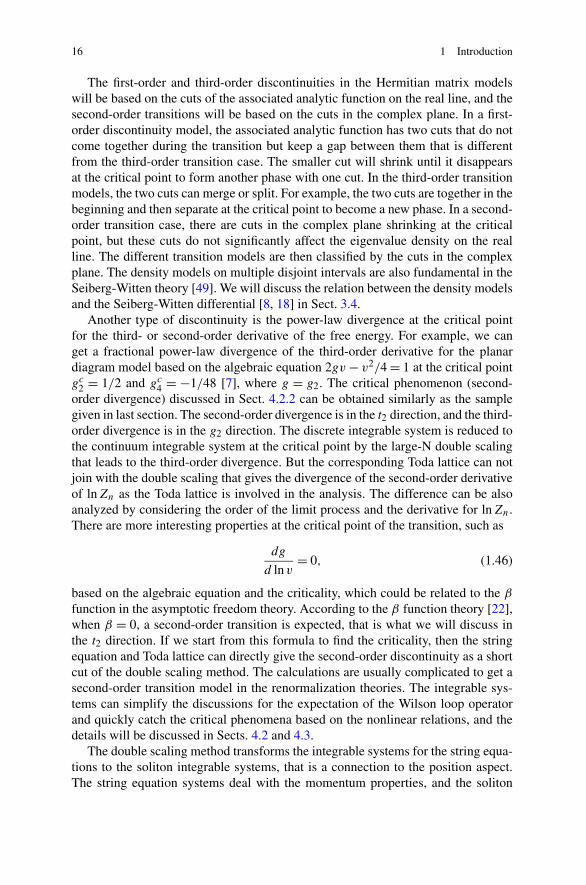
The first-order and third-order discontinuities in the Hermitian matrix modelswill be based on the cuts of the associated analytic function on the real line, and thesecond-order transitions will be based on the cuts in the complex plane. In a first-order discontinuity model, the associated analytic function has two cuts that do notcome together during the transition but keep a gap between them that is differentfrom the third-order transition case. The smaller cut will shrink until it disappearsat the critical point to form another phase with one cut. In the third-order transitionmodels, the two cuts can merge or split. For example, the two cuts are together in thebeginning and then separate at the critical point to become a new phase. In a second-order transition case, there are cuts in the complex plane shrinking at the criticalpoint, but these cuts do not significantly affect the eigenvalue density on the realline. The different transition models are then classified by the cuts in the complexplane. The density models on multiple disjoint intervals are also fundamental in theSeiberg-Witten theory [49]. We will discuss the relation between the density modelsand the Seiberg-Witten differential [8, 18] in Sect. 3.4.
Another type of discontinuity is the power-law divergence at the critical pointfor the third- or second-order derivative of the free energy. For example, we canget a fractional power-law divergence of the third-order derivative for the planardiagram model based on the algebraic equation 2gv − v2/4 = 1 at the critical pointgc2 = 1/2 and gc4 = −1/48 [7], where g = g2. The critical phenomenon (second-order divergence) discussed in Sect. 4.2.2 can be obtained similarly as the samplegiven in last section. The second-order divergence is in the t2 direction, and the third-order divergence is in the g2 direction. The discrete integrable system is reduced tothe continuum integrable system at the critical point by the large-N double scalingthat leads to the third-order divergence. But the corresponding Toda lattice can notjoin with the double scaling that gives the divergence of the second-order derivativeof lnZn as the Toda lattice is involved in the analysis. The difference can be alsoanalyzed by considering the order of the limit process and the derivative for lnZn.There are more interesting properties at the critical point of the transition, such as
dg
d lnv= 0, (1.46)
based on the algebraic equation and the criticality, which could be related to the βfunction in the asymptotic freedom theory. According to the β function theory [22],when β = 0, a second-order transition is expected, that is what we will discuss inthe t2 direction. If we start from this formula to find the criticality, then the stringequation and Toda lattice can directly give the second-order discontinuity as a shortcut of the double scaling method. The calculations are usually complicated to get asecond-order transition model in the renormalization theories. The integrable sys-tems can simplify the discussions for the expectation of the Wilson loop operatorand quickly catch the critical phenomena based on the nonlinear relations, and thedetails will be discussed in Sects. 4.2 and 4.3.
The double scaling method transforms the integrable systems for the string equa-tions to the soliton integrable systems, that is a connection to the position aspect.The string equation systems deal with the momentum properties, and the soliton

1.4 Phase Transitions in the Momentum Aspect 17
systems describe the dynamics in the position aspect. If the steepest descent methodfor the matrix model is considered as a role of an integral transform changing the lat-tice model with many zj variables in scaling to the eigenvalue density model whichis in the scope of Lax pair system, then the double scaling method performs a roleas an inverse transformation to transform the Lax pair system with one z variablefor the string equation to the soliton or equivalent system with another eigenvaluevariable obtained from the z variable in the double scaling. And there are differentdouble scalings to achieve such process depending on the type of the correspondingdensity models with cut(s) on the real line or in the complex plane.
The partition function Zn and the τ function which is a different version of thepartition are in some sense the common part of the two aspects—position and mo-mentum, and they are in the scope of the integrable systems with infinitely manyfreedoms. To reduce to a physical model of finite freedoms using large-N method,the strategy is sensitive because sometimes a method works for this type modelbut not for another model. We need to pay attention, as least, to the limit processfor lnZn, the index range in the formulas, and the stationary point z in the scal-ing. These are often neglected parts. For example, a derivative of lnZn expressedin terms of vn or vn+1 will have different results. The integrable systems provide agood structure to organize the different elements in the system.
The partition function also takes a determinant representation [23, 27] besidesthe integral representations discussed in the previous sections. The τ -function withsuch determinant representation has been studied to describe the integrability in thesoliton theories by using the infinite dimensional Lie algebra [28]. In recent years, itis found that the soliton systems can be applied to derive the phase transition models.The second-order phase transition can be obtained by using the periodic inductionof the parameters in the τ -function in association with the renormalization theoryfor the Ising models, for example, see [35]. The similarity between the periodic in-duction in the soliton systems and the periodic reduction in the recursion formulasof the string equation systems indicates that sometimes the reorganizations of theparticles considered in the renormalization theory can be achieved alternatively byreorganizing the wave functions in the string equation systems under certain condi-tions. Some problems are easy in the position aspect, while others are relatively easyin the momentum aspect, that is a role of the Fourier or integral transform theorywhich connects the position and momentum aspects.
The Fourier transform and Heisenberg uncertainty principle are also fundamen-tal in many other subjects such as the wavelet and signal theories as shown by theuncertainty inequality Δt · Δω ≥ 1/2 of the signal processing for the time t andfrequency ω, for example, see the graduate textbook in mathematics [29] and re-lated literatures. There are many interesting papers in this field, such as [30] for thecomparison between the neighboring fields, and [13] for a connection to the dynam-ical renormalization [40]. According to Palle Jorgensen [29], the visual situation inHeisenberg’s theory was much the same as the one which comes out from the muchlater wavelet constructions. And Heisenberg’s aim for the early quantum theory wasquite different from the later wavelet theories. For reader’s convenience to see howthe uncertainty principle works in the different fields, let us compare the partition

18 1 Introduction
function (generating function) in the matrix model with the mother wavelet func-tion in the wavelet theory. Both of them play a role to handle the two sides of theuncertainty. The mother wavelet is used to define the wavelet transform acting on afunction to change forward and backward like the Fourier transform. The partitionfunction, however, does not act on functions, but accumulates in different ways inlarge scalings to go to the different aspects. The two sides of the uncertainty in thematrix model are handled by the partition in a nonlinear way that is different fromthe direct Fourier transform. The partition model is to formulate the basic physicalsystem for analyzing the states. The Heisenberg uncertainty principle is a commonguidance for many subjects that would motivate researchers in various fields to makenew discoveries.
The integrable systems can be applied to introduce a unified structure to solvethe variational equations for the bifurcation transitions, large-N transitions and di-vergence transitions in the matrix models as explained above, and then the analysison the free energy functions become easier in studying the discontinuity, criticality,order of transition and divergences. In this book we focus on the application of thestring equations and Toda lattices to the discontinuities in the phase transition prob-lems. One should associate the transition models with other physical theories, suchas string theory, unified theory, renormalization group, lattice models, 2D quantumgravity and quantum chromodynamics, for instance, for a better understanding ofthe physical backgrounds.
References
1. Akhiezer, N.I.: Elements of the Theory of Elliptic Functions. Translations of Math. Mono-graphs, vol. 79. AMS, Providence (1990)
2. Bertola, M.: Free energy of the two-matrix model/dToda tau-function. Nucl. Phys. B 669,435–461 (2003)
3. Bertola, M., Marchal, O.: The partition of the two-matrix models as an isomonodromic τ
function. J. Math. Phys. 50, 013529 (2009)4. Bleher, P., Eynard, B.: Double scaling limit in random matrix models and a nonlinear hierarchy
of differential equations. J. Phys. A 36, 3085–3106 (2003)5. Brézin, E., Hikami, S.: Intersection theory from duality and replica. Commun. Math. Phys.
283, 507–521 (2008)6. Brézin, E., Kazakov, V.A.: Exactly solvable field theories of closed strings. Phys. Lett. B 236,
144–150 (1990)7. Brézin, E., Itzykson, C., Parisi, G., Zuber, J.B.: Planar diagrams. Commun. Math. Phys. 59,
35–51 (1978)8. Chekhov, L., Mironov, A.: Matrix models vs. Seiberg–Witten/Whitham theories. Phys. Lett.
B 552, 293–302 (2003)9. Dijkgraaf, R., Moore, G.W., Plesser, R.: The partition function of 2-D string theory. Nucl.
Phys. B 394, 356–382 (1993)10. Douglas, M.R.: Strings in less than one dimension and the generalized KdV hierarchies. Phys.
Lett. B 238, 176–180 (1990)11. Douglas, M.R., Kazakov, V.A.: Large N phase transition in continuum QCD in two-
dimensions. Phys. Lett. B 319, 219–230 (1993)12. Douglas, M.R., Shenker, S.H.: Strings in less than one dimension. Nucl. Phys. B 335, 635–654
(1990)
References 19
13. Dutkay, D.E., Jorgensen, P.E.T.: Hilbert spaces built on a similarity and on dynamical renor-malization. J. Math. Phys. 47(5), 053504 (2006)
14. Eynard, B.: Large-N expansion of the 2 matrix model. J. High Energy Phys. 1, 051 (2003)15. Eynard, B., Orantin, N.: Mixed correlation functions in the 2-matrix model, and the Bethe
ansatz. J. High Energy Phys. 08, 028 (2005)16. Fokas, A.S., Its, A.R., Kitaev, A.V.: Discrete Painlevé equations and their appearance in quan-
tum gravity. Commun. Math. Phys. 142, 313–344 (1991)17. Fuji, H., Mizoguchi, S.: Remarks on phase transitions in matrix models and N = 1 supersym-
metric gauge theory. Phys. Lett. B 578, 432–442 (2004)18. Gorsky, A., Krichever, I., Marshakov, A., Mironov, A., Morozov, A.: Integrability and
Seiberg-Witten exact solution. Phys. Lett. B 355, 466–477 (1995)19. Gross, D.J.: Some remarks about induced QCD. Phys. Lett. B 293, 181–186 (1992)20. Gross, D.J., Migdal, A.A.: Nonperturbative two-dimensional quantum gravity. Phys. Rev. Lett.
64, 127–130 (1990)21. Gross, D.J., Newman, M.J.: Unitary and Hermitian matrices in an external field II: the Kont-
sevich model and continuum Virasoro constraints. Nucl. Phys. B 380, 168–180 (1992)22. Gross, D.J., Witten, E.: Possible third-order phase transition in the large-N lattice gauge the-
ory. Phys. Rev. D 21, 446–453 (1980)23. Harish-Chandra: Differential operators on a semisimple Lie algebra. Am. J. Math. 79, 87–120
(1957)24. Hille, E.: Analytic Function Theory, vols. 1, 2. Chelsea, New York (1974)25. Hisakado, M.: Unitary matrix model and the Painlevé III. Mod. Phys. Lett. A 11, 3001–3010
(1996)26. Hisakado, M., Wadati, M.: Matrix models of two-dimensional gravity and discrete Toda the-
ory. Mod. Phys. Lett. A 11, 1797–1806 (1996)27. Itzykson, C., Zuber, J.B.: The planar approximation II. J. Math. Phys. 21, 411–421 (1980)28. Jimbo, M., Miwa, T., Ueno, K.: Monodromy preserving deformation of linear ordinary differ-
ential equations with rational coefficients. I. Physica D 2, 306–352 (1981)29. Jorgensen, P.E.T.: Analysis and Probability: Wavelets, Signals, Fractals. Graduate Texts in
Mathematics, vol. 234. Springer, New York (2006)30. Jorgensen, P.E.T., Song, M.-S.: Comparison of Discrete and Continuous Wavelet Transforms.
Springer Encyclopedia of Complexity and Systems Science. Springer, Berlin (2008)31. Jurkiewicz, J.: Regularization of one-matrix models. Phys. Lett. B 235, 178–184 (1990)32. Kazakov, V.A., Migdal, A.A.: Induced QCD at large N. Nucl. Phys. B 397, 214–238 (1993)33. Landau, L.D., Lifshitz, E.M.: Statistical Physics, Part 1. Course of Theoretical Physics, vol. 5,
3rd edn. Butterworth–Heinemann, Oxford (1980)34. Lee, M.H.: Solutions of the generalized Langevin equation by a method of recurrence rela-
tions. Phys. Rev. B 26, 2547–2551 (1982)35. Loutsenko, I.M., Spiridonov, V.P.: A critical phenomenon in solitonic Ising chains. SIGMA 3,
059 (2007)36. Marcenko, V.A., Pastur, L.A.: Distribution of eigenvalues for some sets of random matrices.
Mat. Sb. 72(114)(4), 507–536 (1967)37. McKay, B.D.: The expected eigenvalue distribution of a large regular graph. Linear Algebra
Appl. 40, 203–216 (1981)38. McLeod, J.B., Wang, C.B.: Discrete integrable systems associated with the unitary matrix
model. Anal. Appl. 2, 101–127 (2004)39. McLeod, J.B., Wang, C.B.: Eigenvalue density in Hermitian matrix models by the Lax pair
method. J. Phys. A, Math. Theor. 42, 205205 (2009)40. McMullen, C.T.: Complex Dynamics and Renormalization. Annals of Mathematics Studies,
vol. 135. Princeton University Press, Princeton (1994)41. Mehta, M.L.: A method of integration over matrix variables. Commun. Math. Phys. 79, 327–
340 (1981)42. Mehta, M.L.: Random Matrices, 3rd edn. Academic Press, New York (2004)43. Migdal, A.A.: Phase transitions in induced QCD. Mod. Phys. Lett. A 8, 153–166 (1993)

20 1 Introduction
44. Mironov, A., Morozov, A., Semeno, G.W.: Unitary matrix integrals in the framework of gener-alized Kontsevich model. 1. Brézin-Gross-Witten model. Int. J. Mod. Phys. A 11, 5031–5080(1996)
45. Newell, A.C.: Solitons in Mathematics and Physics. SIAM, Philadelphia (1985)46. Periwal, V., Shevitz, D.: Unitary-matrix models as exactly solvable string theories. Phys. Rev.
Lett. 64, 1326–1329 (1990)47. Periwal, V., Shevitz, D.: Exactly solvable unitary matrix models: multicritical potentials and
correlations. Nucl. Phys. B 344, 731–746 (1990)48. Rossi, P., Campostrini, M., Vicari, E.: The large-N expansion of unitary-matrix models. Phys.
Rep. 302, 143–209 (1998)49. Seiberg, N., Witten, E.: Electric-magnetic duality, monopole condensation, and confinement
in N = 2 supersymmetric Yang-Mills theory. Nucl. Phys. B 426, 19–52 (1994). Erratum, ibid.B 430, 485–486 (1994)
50. Sen, S.: Exact solution of the Heisenberg equation of motion for the surface spin in a semi-infinite S = 1
2XY chain at infinite temperatures. Phys. Rev. B 44, 7444–7450 (1991)51. Sengupta, A.M., Mitra, P.P.: Distributions of singular values for some random matrices. Phys.
Rev. E 60, 3389–3392 (1991)52. Shimamune, Y.: On the phase structure of large N matrix models and gauge models. Phys.
Lett. B 108, 407–410 (1982)53. Simon, B.: Orthogonal Polynomials on the Unit Circle, vol. 1: Classical Theory. AMS Collo-
quium Series. AMS, Providence (2005)54. Simon, B.: Orthogonal Polynomials on the Unit Circle, vol. 2: Spectral Theory. AMS Collo-
quium Series. AMS, Providence (2005)55. Stanley, H.E.: Introduction to Phase Transitions and Critical Phenomena. Oxford University
Press, Oxford (1971)56. Szegö, G.: Orthogonal Polynomials, 4th edn. American Mathematical Society Colloquium
Publications, vol. 23. AMS, Providence (1975)57. Vafa, C.: Geometry of grand unification arXiv:0911.3008 (2009)58. Wang, C.B.: Orthonormal polynomials on the unit circle and spatially discrete Painlevé II
equation. J. Phys. A 32, 7207–7217 (1999)59. Wigner, E.P.: Characteristic vectors of bordered matrices with infinite dimensions. Ann. Math.
62, 548–564 (1955)60. Wigner, E.P.: On the distribution of the roots of certain symmetric matrices. Ann. Math. 67,
325–328 (1958)61. Yeomans, J.M.: Statistical Mechanics of Phase Transitions. Oxford University Press, London
(1994)

Chapter 2Densities in Hermitian Matrix Models
Orthogonal polynomials are traditionally studied as special functions in mathemat-ical theories such as in the Hilbert space theory, differential equations and asymp-totics. In this chapter, a new purpose of the generalized Hermite polynomials willbe discussed in detail. The Lax pair obtained from the generalized Hermite polyno-mials can be applied to formulate the eigenvalue densities in the Hermitian matrixmodels with a general potential. The Lax pair method then solves the eigenvaluedensity problems on multiple disjoint intervals, which are associated with scalarRiemann-Hilbert problems for multi-cuts. The string equation can be applied to de-rive the nonlinear algebraic relations between the parameters in the density modelsby reformulating the potential function in terms of the trace function of the coef-ficient matrix obtained from the Lax pair and using the Cayley-Hamilton theoremin linear algebra. The Lax pair method improves the traditional methods for solv-ing the eigenvalue densities by reducing the complexities in finding the nonlinearrelations, and the parameters are then well organized for further analyzing the freeenergy function to discuss the phase transition problems.
2.1 Generalized Hermite Polynomials
Let us consider the Hermitian matrix model with a general potential
V (z)=2m∑
j=0
tj zj , (2.1)
where z is a real or complex variable, tj are real, and t2m > 0 such that the partitionfunction
Zn =∫ ∞
−∞· · ·∫ ∞
−∞e−Σn
i=1V (zi )∏
j<k
(zj − zk)2dz1 · · ·dzn (2.2)
is well defined. The free energy function is defined as [1] E = − limn→∞ 1n2 lnZn.
By the scaling transformation z = n1
2m η and tj = n1− j2m gj , the potential V (z) be-
C.B. Wang, Application of Integrable Systems to Phase Transitions,DOI 10.1007/978-3-642-38565-0_2, © Springer-Verlag Berlin Heidelberg 2013
21

22 2 Densities in Hermitian Matrix Models
comes a new potential W(η) =∑2mj=0 gjη
j . The eigenvalue density ρ(η) on l1 in-
terval(s) Ω =⋃l1j=1[η(j)− , η
(j)+ ] is defined to minimize the free energy function
E =∫
Ω
W(η)ρ(η)dη−∫
Ω
∫
Ω
ln |λ− η|ρ(λ)ρ(η)dλdη. (2.3)
The density ρ(η) is required to satisfy the following conditions [1, 7]:
(i) ρ is non-negative when η ∈Ω ,
ρ(η)≥ 0; (2.4)
(ii) ρ is normalized,∫
Ω
ρ(η)dη = 1; (2.5)
(iii) ρ satisfies the following variational equation for an inner point η of Ω ,
(P)∫
Ω
ρ(λ)
η− λdλ= 1
2W ′(η), (2.6)
where (P) stands for the principal value of the integral, for example,
(P)∫ η+
η−
ρ(λ)
η− λdλ
.= limε→0
(∫ η−ε
η−
ρ(λ)
η− λdλ+
∫ η+
η+ερ(λ)
η− λdλ
)
.
The generalized Hermite polynomials will be applied to find the eigenvalue densityρ(η). The last two conditions will be satisfied based on the asymptotic of an analyticfunction ω(η) as η → ∞, and the first condition needs separate discussions. Thedensity generally takes a form as the product of a polynomial in η and the squareroot of another polynomial in η of degree l ≥ l1, and the parameters in the densityare generally restricted by complicated nonlinear relations that can be obtained byusing the string equation associated with the Hermitian matrix models.
Now, let us use the planar diagram model [1] to briefly explain how the abovebasic concepts are connected each other. For the planar diagram eigenvalue densityshown in Sect. 1.2 for W(η)= 1
2η2 + gη4, if we define
ω(η)=(
1
2+ 4gb2 + 2gη2
)√η2 − 4b2, (2.7)
for η ∈C�Ω where Ω = [−2b,2b] and C stands for the complex plane, then thereis the following asymptotics
ω(η)= 1
2
(η+ 4gη3)− (b2 + 12gb4)1
η+O
(1
η2
)
, (2.8)
as η → ∞. Let Ω∗ =Ω− ∪Ω+ be a closed counterclockwise contour, where Ω−and Ω+ are the lower and upper edges of Ω respectively. By Cauchy theorem,there is
∫Ω∗ ω(η)dη= −(b2 +12gb4)
∫|η|=R
dηη
= −2πi(b2 +12gb4). The analytic
function ω(η) has opposite signs on Ω− and Ω+. If we define ρ(η)= 1πiω(η)|Ω+ ,
then ρ(η) satisfies the normalized condition above if the parameters satisfy
b2 + 12gb4 = 1. (2.9)

2.1 Generalized Hermite Polynomials 23
Further, if Ω∗ is changed to Ω∗ε by just changing the straight lines of the Ω∗ at the
neighborhood of a inner point η of Ω to the small semicircles of ε radius, then wehave
limε→0
∫
Ω∗ε�γε
ω(λ)
λ− ηdλ= lim
ε→0
∫
Ω∗ε
ω(λ)
λ− ηdλ− lim
ε→0
∫
γε
ω(λ)
λ− ηdλ, (2.10)
where γε is the circle of ε radius with center η. Since ω(η) has opposite signs onthe upper and lower edges, the second limit on the right hand side above is zero. Bythe asymptotics above, there is
limε→0
∫
Ω∗ε
ω(λ)
λ− ηdλ= lim
ε→0
∫
Ω∗ε
ω(λ)− 12W
′(λ)λ− η
dλ+ limε→0
∫
Ω∗ε
12W
′(λ)λ− η
dλ
= πiW ′(η). (2.11)
Therefore, ρ(η) satisfies the variational equation given above for the eigenvaluedensity by noting that limε→0
∫Ω∗ε�γε
ω(λ)λ−η dλ= 2πi(P)
∫Ω
ρ(η)η−λ dη. We have shown
the idea to use the ω(η) with the asymptotics to satisfy the conditions for the ρ(η).The question then becomes how to get the ω(η) defined in the complex plane ex-cept the cut(s) with the corresponding asymptotics. The orthogonal polynomials andstring equation can just provide such formulations to construct the ω(η).
In 1991, Fokas, Its and Kitaev [4] obtained that for the potential V (z) = t2z2 +
t4z4, the coefficients vn’s in the recursion formula zpn = pn+1 + vnpn−1 satisfy the
string equation(2t2 + 4t4(vn−1 + vn + vn+1)
)vn = n. (2.12)
If all the vn’s are replaced by n1/2b2 and tj ’s are replaced by n1− j4 gj , and if we
choose g2 = 1/2 and denote g4 = g, then the string equation (2.12) is reduced tothe condition (2.9), which is corresponding to (2.5). The relation between (2.12)and (2.9) indicates that the eigenvalue density problem and the string equation havesome connections. We will see that these relations are so close not only for theiralgebraic formulas but also the roles they play in the corresponding models. Thecondition (2.9) for the eigenvalue density is a property for the exponent of the parti-tion function. The string equation is a property for the exponent n of the orthogonalpolynomials pn(z) = zn + · · ·, that is about the wave function. We will experiencemore about the connections between these equations in the later discussions.
The main question is how to find the formula of the density ρ. It is discussedin [6] by McLeod and Wang in 2009 that the eigenvalue density can be formulatedbased on the square root of the determinant of matrix An(z),
√detAn(z), where
An(z) is the coefficient matrix in the Lax pair
Φn+1 = LnΦn, (2.13)∂
∂zΦn =An(z)Φn. (2.14)
Here Φn(z)= e− 12V (z)(pn(z),pn−1(z))
T , the orthogonal polynomials pn = zn+· · ·are defined on the real line with the weight exp(−V (z)) : 〈pn,pn′ 〉 = hnδn,n′ , and

24 2 Densities in Hermitian Matrix Models
Ln can be obtained from the recursion formula [8] zpn(z)= pn+1(z)+ unpn(z)+vnpn−1(z). The consistency condition for the Lax pair is the string equation whichis a set of two discrete equations for un and vn: 〈pn(z),V ′(z)pn−1(z)〉 = nhn−1 and〈pn(z),V ′(z)pn(z)〉 = 0, where hn/hn−1 = vn. These two relations will be used toderive the conditions (2.5) and (2.6). For the planar diagram model, there is no theequation (2.6) since the potential is an even function.
The coefficient matrix An(z) above is generally a complicated 2 × 2 matrix. Ifwe replace all the un−k−1 and vn−k in the Lax pair by xn and yn respectively, thenAn(z) can be reduced to
An(z)=DnFn(z)D−1n − 1
2V ′(z)I, (2.15)
where the matrix Fn(z) is a linear combination of positive powers of a matrix Jnderived from Ln,
Jn =(
0 1−yn z− xn
)
.
Here Dn = diag(hn,hn−1), and I is the identity matrix. By the Cayley-Hamiltontheorem for Jn as known in the textbooks of linear algebra, we have
(z− xn)I = Jn + ynJ−1n . (2.16)
Applying this relation to V ′(z)I in (2.15), it is found that D−1n An(z)Dn can be
factorized as a product of a polynomial and a simple matrix
D−1n An(z)Dn = f2m−2(z)
(Jn(z)− ynJ
−1n (z)
), (2.17)
where the polynomial f2m−2(z) will be given in the following sections. There is animportant asymptotics
√−det An(z)= 1
2V ′(z)− n
z+O
(1
z2
)
, (2.18)
as z→ ∞ in the complex plane, obtained by using the string equation. This propertywill be applied to satisfy the conditions (2.5) and (2.6). Replacing the variable z and
the parameters tj , xn and yn by n1
2m η, n1− jm gj , n
12m a and n
1m b2 respectively, the
formula of the eigenvalue density ρ(η) on the interval [η−, η+] = [a − 2b, a + 2b]can be obtained by
1
nπ
√det An(z)dz= ρ(η)dη, (2.19)
which follows the unified model discussed in Sect. 1.1. The eigenvalue density prob-lem is then solved when condition (2.4) is satisfied.
The An(z) can be generalized to a new matrix A(l)n (z) to find the eigenvalue den-
sities on multiple disjoint intervals. It should be noted that in some literatures theLax pair is applied to study the asymptotics of un or vn or the related functions,while the method here is to derive the density formula by referring the matrix An(z)
because√−detAn(z) itself also has the same asymptotics (2.18) as z → ∞. The
details of the formulations and the relations to An(z) will be discussed in the fol-lowing sections.

2.2 Integrable System and String Equation 25
2.2 Integrable System and String Equation
For the Hermitian matrix model with potential W(η) =∑mj=1 gjη
2j , we have dis-cussed in last section that the eigenvalue density ρ(η) needs to satisfy the conditions(2.5) and (2.6). In this section, we discuss how to get an analytic function ω(η) withthe asymptotics 1
2W′(η)− 1
ηas η → ∞ in the complex plane, where ′ = ∂/∂η.
Consider the orthogonal polynomials pn(z)= zn + · · · on (−∞,∞) defined by
〈pn,pn′ 〉 ≡∫ ∞
−∞pn(z)pn′(z)e−V (z)dz= hnδn,n′ , (2.20)
where V (z) =∑2mj=0 tj z
j , t2m > 0. We have the following asymptotics e−V (z)/2 ×pn(z)∼ e− 1
2V (z)+n ln z as z→ ∞. This asymptotics gives a hint that the differentialequation for the orthogonal polynomials may help us to find the ω(η). In the fol-lowing, we introduce the basic Lax pair theory to construct the coefficient matrixAn(z).
The orthogonal polynomials satisfy a recursion formula [8],
pn+1(z)+ unpn(z)+ vnpn−1(z)= zpn(z). (2.21)
By multiplying pn−1(z)e−V (z) on both sides of this recursion formula and taking
integral, we get vn = hn/hn−1. This recursion formula will give the first equationin the Lax pair.
For the second equation in the pair, let us consider the differential equation in thez direction. When n ≥ 2m − 1, express the derivative of pn with respect to z as alinear combination of pj ’s,
∂
∂zpn = an,n−1pn−1 + an,n−2pn−2 + · · · + an,0p0, (2.22)
where an,j are independent of z. By integration by parts, there are
an,j hj =∫ ∞
−∞V ′(z)pj (z)pn(z)e−V (z)dz,
(′= ∂/∂z)
for j = 0,1, . . . , n − 1, and an,j = 0 when j < n − 2m + 1 by the orthogonality.Then, by using the recursion formula, ∂
∂zpn can be changed to a linear combination
of pn and pn−1, but the new coefficients are dependent on z.
Denote Φn(z)= e− 12V (z)(pn(z),pn−1(z))
T . By the discussions above, there are
Φn+1 = LnΦn, (2.23)
where
Ln =(z− un −vn
1 0
)
;
and
∂
∂zΦn =An(z)Φn, (2.24)

26 2 Densities in Hermitian Matrix Models
for a matrix An(z). Equations (2.23) and (2.24) are called the Lax pair for the stringequation. This Lax pair structure was given in [4], as well as in [3] (Part 2, Chap. 1).
The Lax pair method for the eigenvalue density starts from the construction ofthe matrix An. For m≥ 1 and n≥ 2m, consider
∂
∂zpn = an,n−1pn−1 + an,n−2pn−2 + · · · + an,n−2m+1pn−2m+1,
∂
∂zpn−1 = an−1,n−2pn−2 + an−1,n−3pn−3 + · · · + an−1,n−2mpn−2m,
where
an′,n′−khn′−k =∫ ∞
−∞V ′(z)pn′−kpn′e−V (z)dz, (2.25)
for n′ = n or n−1, and k = 1,2, . . . ,2m−1, with V ′(z)=∑2mj=1 j tj z
j−1. It followsthat
∂
∂z
(pnpn−1
)
=2m−1∑
k=1
Cn−k(
Pn−kPn−k−1
)
, (2.26)
where
Cn−k =(an,n−khn−k 0
0 an−1,n−k+1hn−k+1
)
, (2.27)
for k = 1, . . . ,2m− 1. And Pj = pj/hj satisfy(
PjPj−1
)
= Jj+1
(Pj+1Pj
)
, Jj+1 =(
0 1−vj+1 z− uj
)
, (2.28)
by using (2.23) and vj+1 = hj+1/hj . Denote Dn = diag(hn,hn−1). The above dis-cussion gives
∂
∂z
(pnpn−1
)
=DnFnD−1n
(pnpn−1
)
, (2.29)
where the matrix Fn is defined by
DnFn = Cn−1Jn +Cn−2Jn−1Jn + · · · +Cn−2m+1Jn−2m+2Jn−2m+3 · · ·Jn. (2.30)
Let I be the 2 × 2 identity matrix. Then, there is
An =DnFnD−1n − 1
2V ′(z)I, n≥ 2m. (2.31)
Let Δ be the operator for the index change acting only on the polynomialsΔkpn = pn+k , where k is an integer. This is the basic idea for the index foldingtechnique for constructing the eigenvalue density on one interval. The recursion for-mula (2.21) becomes (z− un)pn = (Δ+ vnΔ
−1)pn. In the reduced model, we willconsider xn and yn, and (z− xn)
qpn′−k will be associated to
(Δ+ ynΔ
−1)qpn′−k =q∑
r=0
(q
r
)
yrnΔq−2rpn′−k =
q∑
r=0
(q
r
)
yrnpn′−k+q−2r ,

2.2 Integrable System and String Equation 27
for n′ = n or n − 1, k = 1,2, . . . ,2m − 1, and q = 0,1, . . . ,2m − 1. Then by or-thogonality and
V ′(z)=2m∑
j=1
j tj(xn + (z− xn)
)j−1 =2m∑
j=1
j tj
j−1∑
q=0
(j − 1q
)
xj−q−1n (z− xn)
q,
we have that an′,n′−khn′−k is reduced to the following according to (2.25),
2m∑
j=1
j tj
j−1∑
q=0
(j − 1q
)
xj−q−1n
2[q/2]−μq+1∑
r=0
(q
r
)
yrn
∫ ∞
−∞pn′−k+q−2rpn′e−V (z)dz
=2m∑
j=1
j tj
j−1∑
q=0
(j − 1q
)
xj−q−1n
[q/2]−μq∑
r=0
(q
r
)
yrnhn′δq−k−2r,0, (2.32)
for n′ = n or n− 1, where [·] denotes the integer part,
μq = 1 + (−1)q
2={
1, q is even,0, q is odd,
(2.33)
q = 2[q/2] −μq + 1, (2.34)
and for k > 0,
q − k − 2r = 2([q/2] −μq − r
)+ 1 +μq − k < 0, if r > [q/2] −μq,
which implies that δq−k−2r,0 = 0 when r > [q/2]−μq , that is why the upper boundof the index r for the last summation above is changed to [q/2]−μq . Consequently,the DnFn, defined by (2.30) is reduced to
2m−1∑
k=1
2m∑
j=1
j tj
j−1∑
q=0
(j − 1q
)
xj−q−1n
[q/2]−μq∑
r=0
(q
r
)
yrnδq−k−2r,0DnJkn
=2m∑
j=1
j tj
j−1∑
q=0
(j − 1q
)
xj−q−1n
[q/2]−μq∑
r=0
(q
r
)
yrnDnJq−2rn ,
and then Fn is reduced to
Fn =2m∑
j=1
j tj
j−1∑
q=0
(j − 1q
)
xj−q−1n
[q/2]−μq∑
r=0
(q
r
)
yrnJq−2rn , (2.35)
where
Jn =(
0 1−yn z− xn
)
. (2.36)
Let
An(z)=DnFnD−1n − 1
2V ′(z)I, (2.37)

28 2 Densities in Hermitian Matrix Models
which is the matrix we need for the eigenvalue density on one interval. We use thehat symbol such as Jn and An for the reduced models, to distinguish from the Jnand An in the integrable system. Based on the factorization and asymptotics for thismatrix, we will discuss how to find the formula for the eigenvalue density in thelater sections. In the following, we discuss the condition for the parameters that arereduced from the string equation.
By the orthogonality of the polynomials pn(z) = zn + · · · and integration byparts, we have the following string equation,
⟨pn(z),V
′(z)pn−1(z)⟩= nhn−1, (2.38)
⟨pn(z),V
′(z)pn(z)⟩= 0, (2.39)
including two recursion formulas for the un’s and vn’s. The set of (2.38) and (2.39)is called string equation. The string equation is the consistency condition for the Laxpair (2.23) and (2.24). The consistency can be discussed, for example, by referringthe methods in [4, 5]. For the density problems, we only need the equations forrestricting the parameters.
If the differential equation is written in the form
∂
∂zpn = an,npn + an,n−1pn−1 + · · · + an,n−2m+1pn−2m+1,
where an,n = 0, then the formula (2.25) is still true for k = 0. Let us write (2.38)and (2.39) as
an,n−1hn−1 = nhn−1, (2.40)
an,nhn = 0. (2.41)
Based on the reduction (2.32) with n′ = n for k = 1 and k = 0 respectively, in ourmethod for the eigenvalue density on one interval, we need xn and yn to satisfy thefollowing equations
2m∑
j=1
j tj
j−1∑
q=0
(j − 1q
)
xj−q−1n
[q/2]−μq∑
r=0
(q
r
)
yr+1n δq,2r+1 = n, (2.42)
2m∑
j=1
j tj
j−1∑
q=0
(j − 1q
)
xj−q−1n
[q/2]−μq∑
r=0
(q
r
)
yrnδq,2r = 0. (2.43)
Note that δq,2r+1 = 0 when q is even, and δq,2r = 0 when q is odd. Take q = 2p+1,r = p in (2.42), and q = 2p, r = p in (2.43), we get
2m∑
j=2
j tj
[ j2 ]−1∑
p=0
(j − 1
2p+ 1
)(2p+ 1p
)
xj−2p−2n y
p+1n = n, (2.44)
2m∑
j=1
j tj
[ j−12 ]∑
p=0
(j − 1
2p
)(2pp
)
xj−2p−1n y
pn = 0. (2.45)
These two equations will be rescaled to satisfy (2.5) and (2.6).
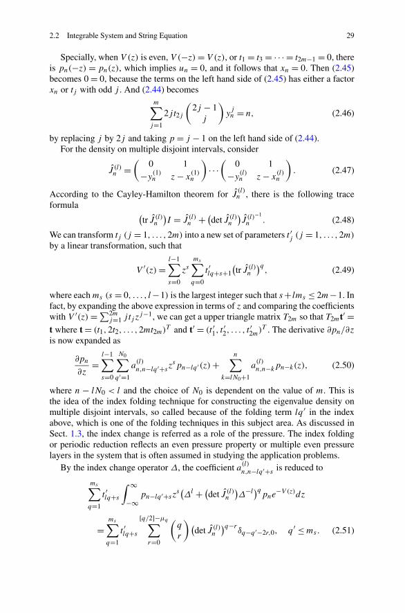
2.2 Integrable System and String Equation 29
Specially, when V (z) is even, V (−z)= V (z), or t1 = t3 = · · · = t2m−1 = 0, thereis pn(−z) = pn(z), which implies un = 0, and it follows that xn = 0. Then (2.45)becomes 0 = 0, because the terms on the left hand side of (2.45) has either a factorxn or tj with odd j . And (2.44) becomes
m∑
j=1
2j t2j
(2j − 1j
)
yjn = n, (2.46)
by replacing j by 2j and taking p = j − 1 on the left hand side of (2.44).For the density on multiple disjoint intervals, consider
J (l)n =(
0 1−y(1)n z− x
(1)n
)
· · ·(
0 1−y(l)n z− x
(l)n
)
. (2.47)
According to the Cayley-Hamilton theorem for J (l)n , there is the following traceformula
(tr J (l)n
)I = J (l)n + (det J (l)n
)J (l)
−1
n . (2.48)
We can transform tj (j = 1, . . . ,2m) into a new set of parameters t ′j (j = 1, . . . ,2m)by a linear transformation, such that
V ′(z)=l−1∑
s=0
zsms∑
q=0
t ′lq+s+1
(tr J (l)n
)q, (2.49)
where each ms (s = 0, . . . , l−1) is the largest integer such that s+ lms ≤ 2m−1. Infact, by expanding the above expression in terms of z and comparing the coefficientswith V ′(z)=∑2m
j=1 j tj zj−1, we can get a upper triangle matrix T2m so that T2mt′ =
t where t = (t1,2t2, . . . ,2mt2m)T and t′ = (t ′1, t ′2, . . . , t ′2m)T . The derivative ∂pn/∂zis now expanded as
∂pn
∂z=
l−1∑
s=0
N0∑
q ′=1
a(l)
n,n−lq ′+szspn−lq ′(z)+
n∑
k=lN0+1
a(l)n,n−kpn−k(z), (2.50)
where n − lN0 < l and the choice of N0 is dependent on the value of m. This isthe idea of the index folding technique for constructing the eigenvalue density onmultiple disjoint intervals, so called because of the folding term lq ′ in the indexabove, which is one of the folding techniques in this subject area. As discussed inSect. 1.3, the index change is referred as a role of the pressure. The index foldingor periodic reduction reflects an even pressure property or multiple even pressurelayers in the system that is often assumed in studying the application problems.
By the index change operator Δ, the coefficient a(l)n,n−lq ′+s is reduced to
ms∑
q=1
t ′lq+s∫ ∞
−∞pn−lq ′+szs
(Δl + (det J (l)n
)Δ−l)qpne−V (z)dz
=ms∑
q=1
t ′lq+s[q/2]−μq∑
r=0
(q
r
)(det J (l)n
)q−rδq−q ′−2r,0, q ′ ≤ms. (2.51)

30 2 Densities in Hermitian Matrix Models
Also, a(l)n,n−lq ′+s for q ′ > ms and a
(l)n,n−k for k = lN0 + 1, . . . , n are reduced to 0
according to the term δq−q ′−2r,0 above. Then we get another reduced matrix
A(l)n (z)=DnF
(l)n D−1
n − 1
2V ′(z)I, (2.52)
where
F (l)n =
l−1∑
s=0
zsms∑
q=1
t ′lq+s+1
[q/2]−μq∑
r=0
(q
r
)(det J (l)n
)r(J (l)n
)q−2r, (2.53)
by referring that (pn−lq ′ ,pn−lq ′−1)T is connected to
Dn
(det J (l)n
)−q ′(J (l)n
)q ′D−1n (pn,pn−1)
T .
The matrix A(l)n (z) will be applied to derive the formula of the density on multi-
ple disjoint intervals to be discussed in Sect. 2.4. The restriction conditions for theparameters are similar to the one-interval case and will be given in Sect. 2.4.
The matrix A(l)n (z) is obtained from An by replacing the un−lq+s−1 and vn−lq+s
by x(s)n and y
(s)n respectively. One may ask whether the uN and vN functions must
have such periodic behaviors. The explanation is that the string equations are appliedto reorganize the wave functions, not the particles. In the momentum aspect, theparameters and the corresponding functions such as uN and vN control the wavefunctions of the random variables, so that the asymptotics of these functions are notdirectly related to the behaviors of the particles. If there is an asymptotic relation,it should be a “relative” asymptotics. These functions are closely connected to themoments of the eigenvalues. Each reduction from the integrable system is not anecessity, but a case of the probability. And the occurrence of each possible case isnot based on certainty principle, but the uncertainty principle. The accumulations ofthe sequences and the distribution of the possibilities would give better explanationsfor the reduction method.
2.3 Factorization and Asymptotics
We have obtained in last section that D−1n AnDn = Fn − 1
2V′(z)I , where Dn =
diag(hn,hn−1). In this section, we are going to show that the matrix Fn − 12V
′(z)Ican be factorized as a product of a polynomial in z of degree 2m− 2 and the matrixJn − ynJ
−1n . The equation det(Jn − ynJ
−1n ) = 0 has only two simply zeros which
will be used as the bounds of the eigenvalue domain. In the following, we will de-note (J−1
n )k by J−kn where k is an integer.
Lemma 2.1 If xn, yn and tj (j = 1, . . . ,2m) satisfy (2.45), then for An(z) definedby (2.37) and μq = (1 + (−1)q)/2, there is

2.3 Factorization and Asymptotics 31
D−1n AnDn = 1
2
2m∑
j=1
j tj
j−1∑
q=0
(j − 1q
)
xj−q−1n
×[q/2]−μq∑
r=0
(q
r
)
yrn(Jq−2rn − (ynJ−1
n
)q−2r). (2.54)
Proof Recall the matrix Jn defined by (2.36),
Jn =(
0 1−yn z− xn
)
.
Applying the Cayley-Hamilton theorem for Jn, there is J 2n − (z− xn)Jn + ynI = 0,
which implies
(z− xn)I = Jn + ynJ−1n . (2.55)
Then by binomial expansion and q = 2[q/2] −μq + 1, we have
(z− xn)qI
=([q/2]−μq∑
r=0
+μq[q/2]∑
r=[q/2]+
2[q/2]−μq+1∑
r=[q/2]+1
)(q
r
)
yrnJq−2rn
=[q/2]−μq∑
r=0
(q
r
)
yrnJq−2rn +μq
(q
[q/2])
y[q/2]n J
q−2[q/2]n
+[q/2]−μq∑
s=0
(q
s
)
yq−sn J
−q+2sn
=[q/2]−μq∑
r=0
(q
r
)
yrn(Jq−2rn + (ynJ−1
n
)q−2r)+μq
(q
[q/2])
y[q/2]n J
q−2[q/2]n ,
where s comes out by the substitution s = q − r , and then replaced by r in the laststep. Since
V ′(z)=2m∑
j=1
j tj
j−1∑
q=0
(j − 1q
)
xj−q−1n (z− xn)
q,
V ′(z)I can be expressed as a linear combination of the positive and negative powersof Jn.
By D−1n AnDn = Fn − 1
2V′(z)I given by (2.37) and (2.35), we then have
D−1n AnDn = 1
2
2m∑
j=1
j tj
j−1∑
q=0
(j − 1q
)
xj−q−1n

32 2 Densities in Hermitian Matrix Models
×[q/2]−μq∑
r=0
(q
r
)
yrn(Jq−2rn − (ynJ−1
n
)q−2r)
= −1
2
2m∑
j=1
j tj
j−1∑
q=0
(j − 1q
)
xj−q−1n μq
(q
[q/2])
y[q/2]n .
Since μq = 1 when q is even, and μq = 0 when q is odd, the last part in the abovevanishes by taking q = 2p and applying (2.45). So we get the result in this lemma. �
Let
αn = z− xn +√(z− xn)2 − 4yn2
, (2.56)
which satisfies
αn + ynα−1n = z− xn, (2.57)
αn − ynα−1n =
√(z− xn)2 − 4yn. (2.58)
And it is easy to check that
ynJ−1n =
(z− xn −1yn 0
)
.
We will need
Jn − ynJ−1n =
(−z+ xn 2−2yn z− xn
)
,
which satisfies√
−det(Jn − ynJ
−1n
)=√(z− xn)2 − 4yn = αn − ynα
−1n . (2.59)
Lemma 2.2 For the Jn defined by (2.36) and k = 1,2, . . . , there are
J kn + yknJ−kn = (αkn + yknα
−kn
)I, (2.60)
and
J kn − yknJ−kn = αkn − yknα
−kn
αn − ynα−1n
(Jn − ynJ
−1n
). (2.61)
Proof By the relations Jn + ynJ−1n = (z− xn)I , and αn + ynα
−1n = z− xn, we have
Jn + ynJ−1n = (αn + ynα
−1n
)I, (2.62)
which is (2.60) for k = 1. Taking square on both sides of (2.62), we get
J 2n + y2
nJ−2n = (α2
n + y2nα
−2n
)I,
which is (2.60) for k = 2.

2.3 Factorization and Asymptotics 33
Now, by mathematical induction, suppose (2.60) is true for k − 1 and k, let usshow it is also true for k + 1. Multiplying (2.60) with (2.62), we get
J k+1n + yk+1
n J−k−1n + yn
(J k−1n + yk−1
n J−k+1n
)
= (αk+1n + yk+1
n α−k−1n
)I + yn
(αk−1n + yk−1
n α−k+1n
)I.
By the assumption, we see that (2.60) is true for k + 1.Equation (2.61) can also be proved by using mathematical induction. It is easy to
check that
J 2n − y2
nJ−2n = (Jn + ynJ
−1n
)(Jn − ynJ
−1n
)= (z− xn)(Jn − ynJ
−1n
),
and then (2.61) is true for k = 1 and 2. Suppose (2.61) is true for k − 1 and k. Weshow it is true for k + 1. Multiplying (2.61) with (2.62), we have
J k+1n − yk+1
n J−k−1n + yn
(J k−1n − yk−1
n J−k+1n
)
= αk+1n − yk+1
n α−k−1n
αn − ynα−1n
(Jn − ynJ
−1n
)+ ynαk−1n − yk−1
n α−k+1n
αn − ynα−1n
(Jn − ynJ
−1n
).
By the assumption, we have that (2.61) is true for k + 1. �
Lemma 2.3 For the αn defined by (2.56) and k = 1,2, . . . , there are
αkn + yknα−kn = 1
2k−1
[ k2 ]∑
s=0
(k
2s
)
(z− xn)k−2s((z− xn)
2 − 4yn)s, (2.63)
and
αkn − yknα−kn
αn − ynα−1n
= 1
2k−1
[ k−12 ]∑
s=0
(k
2s + 1
)
(z− xn)k−2s−1((z− xn)
2 − 4yn)s. (2.64)
Proof By (2.57) and (2.58), we have
αn = 1
2
(z− xn + ((z− xn)
2 − 4yn)1/2)
,
ynα−1n = 1
2
(z− xn − ((z− xn)
2 − 4yn)1/2)
.
Then the binomial formula implies
αkn + yknα−kn
= 1
2k
k∑
j=0
(k
j
)
(z− xn)k−j (((z− xn)
2 − 4yn) j
2 + (−1)j((z− xn)
2 − 4yn) j
2)
= 1
2k−1
[ k2 ]∑
s=0
(k
2s
)
(z− xn)k−2s((z− xn)
2 − 4yn)s,

34 2 Densities in Hermitian Matrix Models
where the terms with odd j are canceled, and the terms with even j are combinedby taking j = 2s. So (2.63) is obtained.
Similarly, there is
αkn − yknα−kn
= 1
2k
k∑
j=0
(k
j
)
(z− xn)k−j (((z− xn)
2 − 4yn) j
2 − (−1)j((z− xn)
2 − 4yn) j
2)
= 1
2k−1
[ k−12 ]∑
s=0
(k
2s + 1
)
(z− xn)k−2s−1((z− xn)
2 − 4yn)s+ 1
2 ,
where the terms with even j are canceled, and the terms with odd j are combinedby taking j = 2s + 1. So the lemma is proved. �
Now, let
f2m−2(z)= 1
2
2m∑
j=1
j tj
j−1∑
q=0
(j − 1q
)
xj−q−1n
[q/2]−μq∑
r=0
(q
r
)yrn
2q−2r−1f (q,r)(z),
(2.65)
where
f (q,r)(z)=[ q−2r−1
2 ]∑
s=0
(q − 2r2s + 1
)
(z− xn)q−2r−2s−1((z− xn)
2 − 4yn)s. (2.66)
Theorem 2.1 If the xn, yn and tj (j = 1, . . . ,2m) satisfy (2.45), then for any z ∈C,there is
D−1n An(z)Dn = f2m−2(z)
(Jn(z)− ynJ
−1n (z)
), (2.67)
where An(z) is defined by (2.37), f2m−2(z) is a polynomial of degree 2m− 2 givenby (2.65), and Jn(z) is given by (2.36).
Proof By Lemma 2.1 and (2.61) in Lemma 2.2, D−1n AnDn is equal to
1
2
2m∑
j=1
j tj
j−1∑
q=0
(j − 1q
)
xj−q−1n
×[q/2]−μq∑
r=0
(q
r
)
yrnαq−2rn − (ynα
−1n )q−2r
αn − ynα−1n
(Jn − ynJ
−1n
).
Applying (2.54) for k = q − 2r in Lemma 2.3 to the above, we then have the re-sult. �
The next goal is to study the asymptotics of (−det(An))1/2 as z → ∞ in the
complex plane. The asymptotics comes out based on (2.44) and (2.45) which arereduced from the string equation.

2.3 Factorization and Asymptotics 35
Theorem 2.2 If the xn, yn and tj (j = 1, . . . ,2m) satisfy (2.44) and (2.45), then asz→ ∞ in the complex plane, there is the asymptotics
√−det An(z)= 1
2V ′(z)− n
z+O
(1
z2
)
, (2.68)
where V (z)=∑2mj=0 tj z
j , t2m > 0 and ′ = ∂/∂z.
Proof By (2.35), (2.36) and (2.37), there is D−1n An(z)Dn ∼ mt2m diag(−z2m−1,
z2m−1) as z → ∞. Since t2m > 0, the branch of the square root is determined by(−det An(z))
1/2 ∼mt2mz2m−1 as z→ +∞ on the real line.
If we take k = q − 2r in (2.61), then
Jq−2rn − (ynJ−1
n
)q−2r = αq−2rn − (ynα
−1n )q−2r
αn − ynα−1n
(Jn − ynJ
−1n
).
Since√
−det(Jn − ynJ−1n )= αn − ynα
−1n , the formula (2.61) implies
√−det
(Jq−2rn − (ynJ−1
n
)q−2r)= αq−2rn − (ynα−1
n
)q−2r.
By (2.54), it follows that
√−det An = 1
2
2m∑
j=1
j tj
j−1∑
q=0
(j − 1q
)
xj−q−1n
×[q/2]−μq∑
r=0
(q
r
)
yrn(αq−2rn − (ynα−1
n
)q−2r). (2.69)
Here, when q = 0, we denote∑−1
r=0 · = 0 for convenience in the discussions. Lets = q − r = ([q/2] − μq − r) + [q/2] + 1 for the terms (ynα−1
n )q−2r above. Wearrive
√−det An = 1
2
2m∑
j=1
j tj
j−1∑
q=0
(j − 1q
)
xj−q−1n
[ [q/2]−μq∑
r=0
(q
r
)
αq−rn
(ynα
−1n
)r
−q∑
s=[q/2]+1
(q
s
)
αq−sn
(ynα
−1n
)s]
.
Furthermore, by the binomial formula we have
√−det An = 1
2
2m∑
j=1
j tj
j−1∑
q=0
(j − 1q
)
xj−q−1n
[(αn + ynα
−1n
)q
−μq
(q
[q/2])
αq−[q/2]n
(ynα
−1n
)[q/2]
− 2q∑
s=[q/2]+1
(q
s
)
ysnα−(2s−q)n
]
.

36 2 Densities in Hermitian Matrix Models
For the first part in the bracket, since αn + ynα−1n = z− xn, it is easy to check that
1
2
2m∑
j=1
j tj
j−1∑
q=0
(j − 1q
)
xj−q−1n
(αn + ynα
−1n
)q = 1
2
2m∑
j=1
j tj zj−1 = 1
2V ′(z).
The second part in the bracket can be dropped off by considering the outside sum-mations and using (2.45). For s = [q/2] + 1 in the third part in the bracket, we havethe following by separating the odd q and even q terms and noticing that q startsfrom q = 1,
2m∑
j=1
j tj
j−1∑
q=1
(j − 1q
)
xj−q−1n
(q
[q/2] + 1
)
y[q/2]+1n α
q−2[q/2]−2n
= α−1n
2m∑
j=1
j tj
[ j2 ]−1∑
p=0
(j − 1
2p+ 1
)(2p+ 1p
)
xj−2p−2n y
p+1n
+ α−2n
2m∑
j=1
j tj
[ j−12 ]∑
p=1
(j − 1
2p
)(2p
p+ 1
)
xj−2p−1n y
p+1n ,
where q = 2p+ 1 when q is odd, and q = 2p when q is even. As z→ ∞, by (2.57)and (2.58), we have
α−1n =
z− xn − (z− xn)(1 − 4yn(z−xn)2 )
1/2
2yn= 1
z− xn+O
(1
(z− xn)2
)
.
Then, combining the discussions above, we obtain√
−det(An)= 1
2
2m∑
j=1
j tj zj−1 − n
z+O
(1
z2
)
,
by using (2.44), and the theorem is proved. �
In the following, we show that (−detAn(z))1/2 has similar asymptotics as dis-
cussed for (−det An(z))1/2 as z → ∞ [6]. Since the restriction conditions for An
and An are different in the asymptotics, separate proofs are needed. The Cauchykernel discussed in [4] is applied in the following proof.
Theorem 2.3 For An defined by (2.31) with n≥ 2m, as z→ ∞, there is√−detAn(z)= 1
2V ′(z)− n
z+O
(1
z2
)
, (2.70)
when the parameters satisfy (2.40).
Proof Denote
pn(z)=∫ ∞
−∞pn(ζ )
e−V (ζ )
ζ − zdζ, and Ψn =
(pn pnpn−1 pn−1
)
e− 12σ3V (z), (2.71)
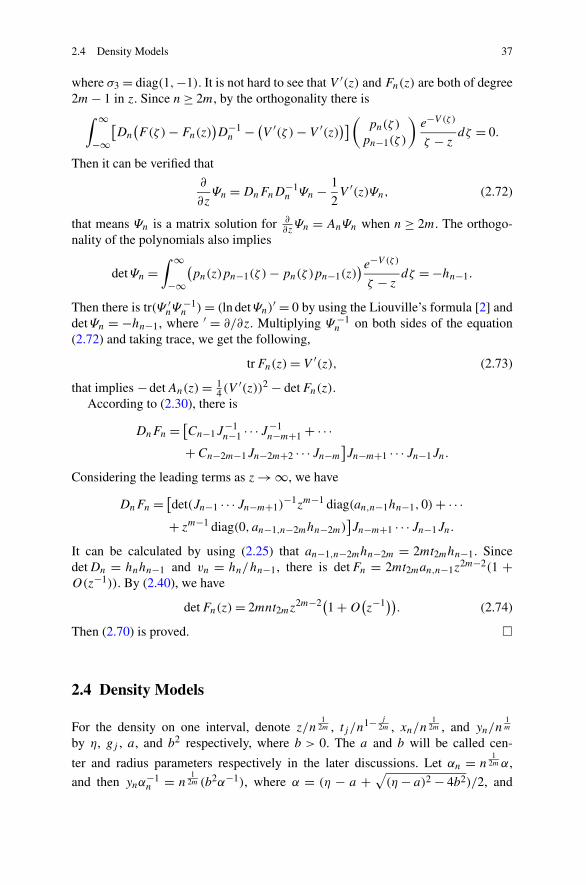
2.4 Density Models 37
where σ3 = diag(1,−1). It is not hard to see that V ′(z) and Fn(z) are both of degree2m− 1 in z. Since n≥ 2m, by the orthogonality there is∫ ∞
−∞[Dn
(F(ζ )− Fn(z)
)D−1n − (V ′(ζ )− V ′(z)
)](
pn(ζ )
pn−1(ζ )
)e−V (ζ )
ζ − zdζ = 0.
Then it can be verified that
∂
∂zΨn =DnFnD
−1n Ψn − 1
2V ′(z)Ψn, (2.72)
that means Ψn is a matrix solution for ∂∂zΨn = AnΨn when n ≥ 2m. The orthogo-
nality of the polynomials also implies
detΨn =∫ ∞
−∞(pn(z)pn−1(ζ )− pn(ζ )pn−1(z)
)e−V (ζ )
ζ − zdζ = −hn−1.
Then there is tr(Ψ ′nΨ
−1n )= (ln detΨn)′ = 0 by using the Liouville’s formula [2] and
detΨn = −hn−1, where ′ = ∂/∂z. Multiplying Ψ−1n on both sides of the equation
(2.72) and taking trace, we get the following,
trFn(z)= V ′(z), (2.73)
that implies −detAn(z)= 14 (V
′(z))2 − detFn(z).According to (2.30), there is
DnFn = [Cn−1J−1n−1 · · ·J−1
n−m+1 + · · ·+Cn−2m−1Jn−2m+2 · · ·Jn−m
]Jn−m+1 · · ·Jn−1Jn.
Considering the leading terms as z→ ∞, we have
DnFn = [det(Jn−1 · · ·Jn−m+1)−1zm−1 diag(an,n−1hn−1,0)+ · · ·
+ zm−1 diag(0, an−1,n−2mhn−2m)]Jn−m+1 · · ·Jn−1Jn.
It can be calculated by using (2.25) that an−1,n−2mhn−2m = 2mt2mhn−1. SincedetDn = hnhn−1 and vn = hn/hn−1, there is detFn = 2mt2man,n−1z
2m−2(1 +O(z−1)). By (2.40), we have
detFn(z)= 2mnt2mz2m−2(1 +O
(z−1)). (2.74)
Then (2.70) is proved. �
2.4 Density Models
For the density on one interval, denote z/n1
2m , tj /n1− j2m , xn/n
12m , and yn/n
1m
by η, gj , a, and b2 respectively, where b > 0. The a and b will be called cen-
ter and radius parameters respectively in the later discussions. Let αn = n1
2m α,
and then ynα−1n = n
12m (b2α−1), where α = (η − a + √
(η− a)2 − 4b2)/2, and

38 2 Densities in Hermitian Matrix Models
b2α−1 = (η − a − √(η− a)2 − 4b2)/2. By Theorem 2.1, it follows that for z ∈C�[xn − 2
√yn, xn + 2
√yn ],
√−det An(z)= n1− 1
2m k2m−2(η)
√(η− a)2 − 4b2, η ∈C�[a − 2b, a + 2b],
(2.75)
where
k2m−2(η)=2m∑
j=1
jgj
j−1∑
q=0
(j − 1q
)
aj−q−1[ q2 ]−μq∑
r=0
(q
r
)b2r
2q−2rk(q,r)(η), (2.76)
and
k(q,r)(η)=[ q−2r−1
2 ]∑
s=0
(q − 2r2s + 1
)
(η− a)q−2r−2s−1((η− a)2 − 4b2)s , (2.77)
where(mn
)= m!/(n!(m− n)!), μq = (1 + (−1)q)/2, and [·] stands for the integerpart.
Define an analytic function [6]
ω(η)= k2m−2(η)
√(η− a)2 − 4b2, η ∈C�[a − 2b, a + 2b]. (2.78)
The parameters a, b and gj (j = 1, . . . ,2m) are required to satisfy the conditions:
(i) When η ∈ [η−, η+],k2m−2(η)≥ 0; (2.79)
(ii)2m∑
j=2
jgj
[ j2 ]−1∑
p=0
(j − 1
2p+ 1
)(2p+ 1p
)
aj−2p−2b2p+2 = 1; (2.80)
(iii)2m∑
j=1
jgj
[ j−12 ]∑
p=0
(j − 1
2p
)(2pp
)
aj−2p−1b2p = 0. (2.81)
By Theorem 2.2, if a, b, and gj (j = 1, . . . ,2m) satisfy (2.80) and (2.81), thenfor η ∈ C�[a − 2b, a + 2b] there is
ω(η)= 1
2
2m∑
j=1
jgj
j−1∑
q=0
(j − 1q
)
aj−q−1[q/2]−μq∑
r=0
(q
r
)
b2r(αq−2r − (b2α−1)q−2r).
(2.82)
As η → ∞, there is
ω(η)= 1
2W ′(η)− 1
η+O
(1
η2
)
. (2.83)

2.4 Density Models 39
In (2.82), the index j actually starts from j = 2, and index q starts from 1. We keepthis form just for convenience in the later discussion for free energy when we use(2.81) where j is from j = 1 and p is from p = 0. Let
ρ(η)= 1
πk2m−2(η)
√(η+ − η)(η− η−), η ∈ [η−, η+], (2.84)
where η− = a− 2b,η+ = a+ 2b, b > 0, and k2m−2(η) is given by (2.76). By (2.78)and (2.84), there is
ω(η)|[η−,η+]± = ±πiρ(η)|[η−,η+], (2.85)
where [η−, η+]+ and [η−, η+]− stand for the upper and lower edges of the interval[η−, η+] respectively. Since ρ(η) is non-negative, we also need
k2m−2(η)≥ 0, (2.86)
for η ∈ [η−, η+].For the density on multiple disjoint intervals, consider
J (l) =(
0 1−b2
1 η− a1
)
· · ·(
0 1−b2
l η− al
)
, (2.87)
where l ≥ 1. According to the Cayley-Hamilton theorem for J (l), choose α(l) =(Λ+
√Λ2 − 4b(l)2)/2, where Λ=Λ(η)= trJ (l), b(l)
2 = detJ (l) and b(l) > 0. Wecan transform gj (j = 1, . . . ,2m) into a new set of parameters g′
j (j = 1, . . . ,2m)
by a linear transformation so that W ′(η) =∑l−1s=0 η
s∑ms
q=0 g′lq+s+1Λ
q , where eachms (s = 0, . . . , l − 1) is the largest integer such that s + lms ≤ 2m− 1.
Define another analytic function [6]
ωl(η)= 1
2
l−1∑
s=0
ηsms∑
q=1
g′lq+s+1
[q/2]−μq∑
r=0
(q
r
)
b(l)2r(
α(l)q−2r − (b(l)2α(l)−1)q−2r)
,
(2.88)
for η in the outside of the cuts to be discussed in the following. Then there is ωl(η)=12W
′(η)+ y(η), where −y(η) is equal to
l−1∑
s=0
ηsms∑
q=0
g′lq+s+1
[μq
2
(q
[q/2])
b(l)2[q/2]
α(l)q−2[q/2]
+q∑
r=[q/2]+1
(q
r
)
b(l)2rα(l)
q−2r
]
. (2.89)
It is the same argument as discussed for ω(η) that if the parameters satisfy theconditions
[ml−1−12 ]∑
p=0
g′2lp+2l
(2p+ 1p
)
b(l)2p+2 = 1, (2.90)

40 2 Densities in Hermitian Matrix Models
Fig. 2.1 Multiple cuts andtheir upper and lower edges
[ms2 ]∑
p=0
g′2lp+s+1
(2pp
)
b(l)2p = 0, (2.91)
for s = 0,1, . . . , l − 1, then
ωl(η)= 1
2W ′(η)− 1
η+O
(1
η2
)
, (2.92)
as η → ∞.
Now, consider the cuts for ωl(η), determined by α(l)−b(l)2α(l)
−1which is equal
to√Λ2 − 4b(l)2. Equation Λ2 − 4b(l)
2 = 0 has 2l roots, real or complex. If thereis a complex root, its complex conjugate is also a root. If there is repeated root, thefactor can be moved out from the inside of the square root in the expression of ωl(η).
Therefore, without loss of generality, we consider the equation Λ2 − 4b(l)2 = 0 has
2l1 simple real roots η(s)− , η(s)+ , s = 1, . . . , l1, and 2l2 simple complex roots ηs, ηs ,
s = 1, . . . , l2, where ηs is the complex conjugate of ηs , Imηs > 0, and l = l1 + l2.Suppose the real roots are so ordered that [η(s)− , η
(s)+ ], s = 1, . . . , l1, form a set of
disjoint intervals, Ω =⋃l1s=1[η(s)− , η
(s)+ ], see Fig. 2.1. Define
ρl(η)= Re1
πiωl(η)
∣∣∣∣Ω+
, (2.93)
for η ∈ Ω as the general eigenvalue density on multiple disjoint intervals in theHermitian matrix models. It can be seen that when l = l1 = 1, ω1 = ω, ρ1(η) =ρ(η), and the conditions (2.90) and (2.91) become (2.80) and (2.81) respectively.
Choose l2 points η(0)s on the real line outside Ω , such that the straight lines Γs ’s,each one connecting ηs and η(0)s for s = 1, . . . , l2, do not intersect each other. Now,ωl(η) is well defined and analytic in the outside of Ω ∪⋃l2
s=1(Γs ∪ Γs), where Γsis the straight line connecting ηs and η
(0)s . Let Γ ∗
s be the closed counterclockwisecontour along the edges of Γs ∪ Γs , and define
Is =∫
Γ ∗s
ωl(η)dη, and Is (η)=∫
Γ ∗s
ωl(λ)
λ− ηdλ, η ∈Ω,
for s = 1, . . . , l2. According to the definition of Γ ∗s , Is and Is (η) are real.
Theorem 2.4 If the parameters as, bs(s = 1, . . . , l), and gj (j = 1, . . . ,2m) satisfythe conditions (2.90) and (2.91), then ρl(η) defined by (2.93) on Ω satisfies (2.5)and (2.6).

2.4 Density Models 41
Proof Let Γ be a large counterclockwise circle of radius R, and Ω∗ be the unionof closed counterclockwise contours around the upper and lower edges of all theintervals in Ω . Then by Cauchy theorem and (2.92),
∫
Ω∗
(
ωl(η)− 1
2W ′(η)
)
dη+l2∑
s=1
Is =∫
Γ
(
ωl(η)− 1
2W ′(η)
)
dη→ −2πi,
as R → ∞, which implies∫Ωρ(η)dη = 1 by (2.85),
∫Ω∗ W ′(η)dη = 0, and Is are
real. So ρ(η) satisfies the condition (2.5).Change the Ω− and Ω+ discussed above just at η ∈Ω as semicircles of ε radius.
By (2.92) and∫Γ ∗s
W ′(λ)λ−η dλ= 0, there is
1
2πi
∫
Ω∗
ωl(λ)− 12W
′(λ)λ− η
dλ+ 1
2πi
l2∑
s=1
Is = 1
2πi
∫
Γ
ωl(λ)− 12W
′(λ)λ− η
dλ→ 0,
as R → ∞. Then taking the real parts of both sides, we get
1
2W ′(η)= 1
2π
∫
Ω∗
Re 1iωl(λ)
λ− ηdλ→ (P)
∫
Ω
ρ(λ)
η− λdλ,
as ε → 0 by using (2.93). �
By the discussions above, it can be seen that when l2 = 0, as, bs (s = 1, . . . , l),and gj (j = 1, . . . ,2m) satisfy the relations (2.90) and (2.91), then y(η) =ωl(η)− 1
2W′(η) satisfies the following relations: y(η) is analytic when η ∈ C�Ω;
y(η)|Ω+ + y(η)|Ω− = −W ′(η);y(η) → 0, as η → ∞. These relations are impor-tant in complex analysis, called scalar Riemann-Hilbert problem. If the parametersas and bs can be chosen such that
(trJ (l)
)2 − 4 detJ (l) =l∏
j=1
(η− η
(j)−)(η− η
(j)+), (2.94)
then the density models and the corresponding scalar Riemann-Hilbert problems canbe well solved. Note that the left hand side of (2.94) is also equal to −det(J (l) −(detJ (l))J (l)
−1) by considering (J (l)−√
detJ (l))(J (l)+√detJ (l)) and calculating
the determinants.By Theorem 2.3, when n ≥ 2m and the parameters satisfy (2.40), the σn(z) de-
fined by
σn(z)= 1
πRe√
detAn(z), −∞< z <∞, (2.95)
satisfies∫∞−∞ σn(z)dz = n and (P)
∫∞−∞
σn(z′)
z−z′ dz′ = 1
2V′(z), as the level density [7],
that is consistent with the unified model discussed in Sect. 1.1. When the densityinvolves the parameter n, the string equation and the initial conditions when n isless than 2m need to be considered to calculate the functions un and vn.

42 2 Densities in Hermitian Matrix Models
2.5 Special Densities
When m= 1 and W(η)= η2, there is
ρ(η)= 1
π
√2 − η2, (2.96)
for η ∈ [−√2,
√2], which is the well known Wigner semicircle.
When m= 2 and W(η)= g2η2 + g4η
4, by the discussions before we have
ρ(η)= 1
π
(g2 + 2g4
(η2 + 2b2))
√4b2 − η2, (2.97)
for η ∈ [−2b,2b], with the restriction conditions
g2 + 2g4(η2 + 2b2)≥ 0, η ∈ [−2b,2b], (2.98)
2g2b2 + 12g4b
4 = 1. (2.99)
The results are consistent with the case W(η) = 12η
2 + gη4 obtained by Brezin,Itzykson, Parisi and Zuber [1] that
ρ(η)= 1
π
(1
2+ 4gb2 + 2gη2
)√4b2 − η2, (2.100)
for η ∈ [−2b,2b], where
b2 + 12gb4 = 1. (2.101)
When W(η) = g0 + g1η + g2η2 + g3η
3 + g4η4, by Theorem 2.4, we have the
following general density formula
ρ(η)= 1
2π
(2g2 + 3g3(η+ a)+ 4g4
(η2 + aη+ a2 + 2b2))
√4b2 − (η− a)2,
(2.102)
where the parameters satisfy the following conditions
2g2 + 3g3(η+ a)+ 4g4(η2 + aη+ a2 + 2b2)≥ 0, η ∈ [η−, η+], (2.103)
2g2b2 + 6g3ab
2 + 12g4(a2 + b2)b2 = 1, (2.104)
g1 + 2g2a + 3g3(a2 + 2b2)+ 4g4a
(a2 + 6b2)= 0, (2.105)
obtained from (2.4), (2.5) and (2.6), where η− = a − 2b, η+ = a + 2b. The densityformula and the conditions coincide with the results (45) and (46) in [1] for the caseW(η)= 1
2η2 + g3η
3.When g1 = g2 = 0, i.e., W(η)= g0 + g3η
3 + g4η4, the conditions become
3g3(η+ a)+ 4g4(η2 + aη+ a2 + 2b2)≥ 0, η ∈ [η−, η+], (2.106)
g3 = − 8a(a2 + 6b2)
3b2(5a4 + 3(a2 − 4b2)2), (2.107)
g4 = 2(a2 + 2b2)
b2(5a4 + 3(a2 − 4b2)2). (2.108)

2.5 Special Densities 43
The first condition (2.106) is satisfied if and only if τ = 4b2
a2 is restricted in the
interval 0 < τ ≤ τ− or τ+ ≤ τ , where τ+ = 1 + √5, and τ− is uniquely determined
by the conditions: 0 < τ− < 1/2 and 1 − 2τ 1/2− + 3
4τ2− = 0. Approximately we have
τ− ≈ 0.28 and τ+ ≈ 3.24. The density function in this case can be further rescaledinto the following forms. Let η = ax and τ = c2 (c > 0). Then
ρ(η)dη = 16
π
(xc
− c2 )
2 + x2−12
5 + 3(1 − c2)2
√c2 − (x − 1)2dx, (2.109)
for x ∈ [1 − c,1 + c], where c ∈ (0, c−] ∪ [c+,∞), c− = √τ− and c+ = √
τ+. Onthe other hand, if η = −ax and τ = c2 (c > 0), then
ρ(η)dη = 16
π
(xc
+ c2 )
2 + x2−12
5 + 3(1 − c2)2
√c2 − (x + 1)2dx, (2.110)
for x ∈ [−1 − c,−1 + c], where c ∈ (0, c−] ∪ [c+,∞), c− = √τ− and c+ = √
τ+.The density on two disjoint intervals can also be obtained by using the method
discussed before. Briefly, we have
ρ(η)= 1
2π
(3g3 + 4g4(a1 + a2 + η)
)Re√
4b21b
22 − ((η− a1)(η− a2)− b2
1 − b22
)2,
(2.111)
where −∞< η <∞, and
4g4b21b
22 = 1, (2.112)
2g2 + (3g3 + 4g4(a1 + a2))(a1 + a2)− 4g4
(a1a2 − b2
1 − b22
)= 0, (2.113)
g1 − (3g3 + 4g4(a1 + a2))(a1a2 − b2
1 − b22
)= 0. (2.114)
It can be checked that if we take a1 = a2 = a and b1 = b2 = b in the above, thena and b satisfy (2.104) and (2.105). In addition, the non-negative condition for thisρ(η) will be discussed in next chapter.
When m= 3, by Theorem 2.4, there is
ρ(η)= 1
π
(g2 + 2g4
(η2 + 2b2)+ 3g6
(η4 + 2b2η2 + 6b4))
√4b2 − η2, (2.115)
for η ∈ [−2b,2b], and (2.103) and (2.104) become
g2 + 2g4(η2 + 2b2)+ 3g6
(η4 + 2b2η2 + 6b4)≥ 0, η ∈ [−2b,2b], (2.116)
2g2b2 + 12g4b
4 + 60g6b6 = 1. (2.117)
Generally, for the symmetric density with the potential W(η)=∑mj=1 gjη
2j , wehave the following by Theorem 2.4
ρ(η)= 1
πk2m−2(η)
√4b2 − η2, η ∈ [−2b,2b], (2.118)
where
k2m−2(η)=m∑
j=1
jg2j
j∑
p=1
(2j − 1j − p
)b2(j−p)
4p−1
p−1∑
s=0
(2p− 12s + 1
)
η2(p−s−1)(η2 − 4b2)s ,
(2.119)
44 2 Densities in Hermitian Matrix Models
and
k2m−2(η)≥ 0, η ∈ [−2b,2b], (2.120)m∑
j=1
2jg2j
(2j − 1j
)
b2j = 1. (2.121)
Here, the formula (2.119) is obtained from (2.76) and (2.77) by choosing g1 = g3 =· · · = g2m−1 = 0 and a = 0 first, then replacing j by 2j and taking the substitutionsq = 2j − 1 and r = j − p. By the asymptotics (2.83), we also have that for largeR > 0, there is
k2m−2(η)= 1
2πi
∮
|λ|=Rω(λ)√λ2 − 4b2
dλ
λ− η= 1
2πi
∮
|λ|=R
12W
′(λ)√λ2 − 4b2
dλ
λ− η.
(2.122)
References
1. Brézin, E., Itzykson, C., Parisi, G., Zuber, J.B.: Planar diagrams. Commun. Math. Phys. 59,35–51 (1978)
2. Coddington, E.A., Levinson, N.: Theory of Ordinary Differential Equations. McGraw-Hill,New York (1955)
3. Faddeev, L., Takhtajan, L.: Hamiltonian Methods in the Theory of Solitons. Springer, Berlin(1986)
4. Fokas, A.S., Its, A.R., Kitaev, A.V.: Discrete Painlevé equations and their appearance in quan-tum gravity. Commun. Math. Phys. 142, 313–344 (1991)
5. Jimbo, M., Miwa, T.: Monodromy preserving deformation of linear ordinary differential equa-tions with rational coefficients. II. Physica D 2, 407–448 (1981)
6. McLeod, J.B., Wang, C.B.: Eigenvalue density in Hermitian matrix models by the Lax pairmethod. J. Phys. A, Math. Theor. 42, 205205 (2009)
7. Mehta, M.L.: Random Matrices, 3rd edn. Academic Press, New York (2004)8. Szegö, G.: Orthogonal Polynomials, 4th edn. American Mathematical Society Colloquium Pub-
lications, vol. 23. AMS, Providence (1975)

Chapter 3Bifurcation Transitions and Expansions
It is believed in matrix model theory that when the eigenvalue density on one in-terval is split to a new density on two disjoint intervals, a phase transition occurs.The complexity for the mathematical details of this physical phenomenon comesnot only from the elliptic integral calculations, but also from the organization ofthe parameters in the model. Generally, the elliptic integrals do not have simpleanalytic formulations for discussing the transition. The string equations can be ap-plied to find the critical point for the transition from the parameter bifurcation, andthe bifurcation clearly separates the different phases for analyzing the free energy.Based on the expansion method for elliptic integrals, the third-order bifurcationtransition for the Hermitian matrix model with a general quartic potential is dis-cussed in this chapter by applying the nonlinear relations obtained from the stringequations. The density on multiple disjoint intervals for higher degree potentialand the corresponding free energy are discussed in association with the Seiberg-Witten differential. In the symmetric cases for the quartic potential, the third-orderphase transitions are explained with explicit formulations of the free energy func-tion.
3.1 Free Energy for the One-Interval Case
In this section, we discuss the free energy [16]
E =∫
Ω
W(η)ρ(η)dη−∫
Ω
∫
Ω
ln |λ− η|ρ(λ)ρ(η)dλdη, (3.1)
for the density
ρ(η)= 1
πk2m−2(η)
√(η+ − η)(η− η−), η ∈Ω = [η−, η+], (3.2)
C.B. Wang, Application of Integrable Systems to Phase Transitions,DOI 10.1007/978-3-642-38565-0_3, © Springer-Verlag Berlin Heidelberg 2013
45

46 3 Bifurcation Transitions and Expansions
obtained in Sect. 2.4 with the parameter conditions
2m∑
j=2
jgj
[ j2 ]−1∑
p=0
(j − 1
2p+ 1
)(2p+ 1p
)
aj−2p−2b2p+2 = 1, (3.3)
2m∑
j=1
jgj
[ j−12 ]∑
p=0
(j − 1
2p
)(2pp
)
aj−2p−1b2p = 0. (3.4)
The following discussions are based on the results in [15]. As always, we assumeρ(η) is non-negative in the discussions.
Lemma 3.1 For ρ(η) defined by (3.2) on [η−, η+] with the parameters a, b andgj (j = 1, . . . ,2m) satisfying the conditions (3.3) and (3.4), there is
∫ η+
η−ηkρ(η)dη =
2m∑
j=2
jgj
j−1∑
q=1
(j − 1q
)
aj−q−1bq+1
×[q/2]−μq∑
r=0
(q
[q/2] + r + 1
)
R2r+μq+1,k (3.5)
where
Rl,k = i
π
∫ π
−π(a + 2b cos θ)ke−ilθ sin θdθ, (3.6)
with l = 2r +μq + 1 and μq = (1 + (−1)q)/2.
Proof Let Ω∗ be the closed counterclockwise contour around lower and upperedges of [η−, η+], and Γ be a large counterclockwise circle. Since Ω∗ is coun-terclockwise, by the relation ω(η)|[η−,η+]± = ±πiρ(η)|[η−,η+] and the Cauchy the-orem we have
∫ η+
η−ηkρ(η)dη = − 1
2πi
∫
Ω∗ηkω(η)dη = − 1
2πi
∫
Γ
ηkω(η)dη.
So the problem becomes the calculation of the integral∫Γηkω(η)dη.
By using the binomial formula and∫Γηk(α+ b2α−1)qdη= ∫
Γηk(η− a)qdη=
0, we can obtain∫ η+
η−ηkρ(η)dη = 1
2πi
2m∑
j=2
jgj
j−1∑
q=1
(j − 1q
)
aj−q−1
×q∑
s=[q/2]+1
(q
s
)
b2s∫
Γ
ηkα−(2s−q)dη. (3.7)
Notice that the index q is changed to start from 1, and j is changed to start from 2.

3.1 Free Energy for the One-Interval Case 47
On Ω∗, there is η = a + 2b cos θ,−π ≤ θ ≤ π , where a = (η+ + η−)/2 and2b = (η+ − η−)/2 > 0. Then α−1 = b−1e−iθ , where the square root takes positiveand negative imaginary value on upper and lower edge of [η−, η+] respectively. ByCauchy theorem, the integral along Γ can be changed to along Ω∗, that implies
∫
Γ
ηkα−(2s−q)dη = −2bq−2s+1∫ π
−π(a + 2b cos θ)ke−i(2s−q)θ sin θdθ.
Let r = s−[q/2]−1 in (3.7). Because the range of s is from [q/2]+1 to q , and q =2[q/2]−μq +1, the range of r is from 0 to [q/2]−μq . Since 2s−q = 2r+μq +1,this lemma is proved. �
Lemma 3.2 For ρ(η) defined by (3.2) on [η−, η+] with the parameters a, b andgj (j = 1, . . . ,2m) satisfying the conditions (3.3) and (3.4), there is
∫ η+
η−ln |η− a|ρ(η)dη
= ln(2b)−2m∑
j=2
jgj
j−1∑
q=1
(j − 1q
)
aj−q−1bq+1
×[q/2]−μq∑
r=0
(q
[q/2] + r + 1
)
Θ2r+μq+1 (3.8)
where
Θl = Rei
π
∫ π
0θeiθ
[(eiθ +
√e2iθ − 1
)l − (eiθ −√e2iθ − 1
)l]dθ, (3.9)
with l = 2r +μq + 1 and μq = (1 + (−1)q)/2.
Proof Let γ = γ1 ∪ γ2 ∪ γ3 be a closed counterclockwise contour, where γ1 is theupper edges of [η−, a], γ2 is the upper edges of [a,η+], and γ3 is the semi-circle ofradius 2b with center a. Applying Cauchy theorem for ln(η− a)ω(η), we have∫
γ1
(ln |η− a| + πi)ω(η)dη+∫
γ2
ln |η− a|ω(η)dη+∫
γ3
ln(2beiθ
)ω(η)dη = 0.
When η ∈ γ1 ∪ γ2, ω(η)= πiρ(η). Then taking imaginary part for the above equa-tion, we get
∫ η+
η−ln |η− a|ρ(η)dη− ln(2b)+ 1
πRe∫
γ3
θω(η)dη= 0, (3.10)
where we have used∫γ3ω(η)dη = − ∫
γ1∪γ2ω(η)dη = −πi ∫
γ1∪γ2ρ(η)dη = −πi.
So the problem becomes the calculation of the integral∫γ3θω(η)dη.
Rewrite the formula of ω(η) given in Sect. 2.4 for the one-interval case as
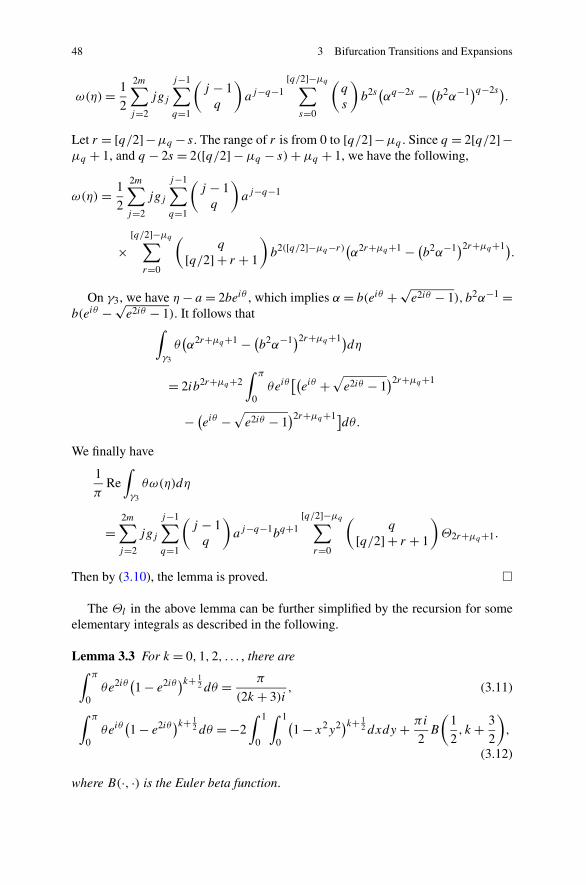
48 3 Bifurcation Transitions and Expansions
ω(η)= 1
2
2m∑
j=2
jgj
j−1∑
q=1
(j − 1q
)
aj−q−1[q/2]−μq∑
s=0
(q
s
)
b2s(αq−2s − (b2α−1)q−2s).
Let r = [q/2]−μq − s. The range of r is from 0 to [q/2]−μq . Since q = 2[q/2]−μq + 1, and q − 2s = 2([q/2] −μq − s)+μq + 1, we have the following,
ω(η) = 1
2
2m∑
j=2
jgj
j−1∑
q=1
(j − 1q
)
aj−q−1
×[q/2]−μq∑
r=0
(q
[q/2] + r + 1
)
b2([q/2]−μq−r)(α2r+μq+1 − (b2α−1)2r+μq+1).
On γ3, we have η− a = 2beiθ , which implies α = b(eiθ + √e2iθ − 1), b2α−1 =
b(eiθ − √e2iθ − 1). It follows that
∫
γ3
θ(α2r+μq+1 − (b2α−1)2r+μq+1)
dη
= 2ib2r+μq+2∫ π
0θeiθ
[(eiθ +
√e2iθ − 1
)2r+μq+1
− (eiθ −√e2iθ − 1
)2r+μq+1]dθ.
We finally have
1
πRe∫
γ3
θω(η)dη
=2m∑
j=2
jgj
j−1∑
q=1
(j − 1q
)
aj−q−1bq+1[q/2]−μq∑
r=0
(q
[q/2] + r + 1
)
Θ2r+μq+1.
Then by (3.10), the lemma is proved. �
The Θl in the above lemma can be further simplified by the recursion for someelementary integrals as described in the following.
Lemma 3.3 For k = 0,1,2, . . . , there are∫ π
0θe2iθ (1 − e2iθ )k+ 1
2 dθ = π
(2k + 3)i, (3.11)
∫ π
0θeiθ
(1 − e2iθ )k+ 1
2 dθ = −2∫ 1
0
∫ 1
0
(1 − x2y2)k+ 1
2 dxdy + πi
2B
(1
2, k + 3
2
)
,
(3.12)
where B(·, ·) is the Euler beta function.

3.1 Free Energy for the One-Interval Case 49
Proof The first equation in this lemma can be easily verified by using integrationby parts,
∫ π
0θe2iθ (1 − e2iθ )k+ 1
2 dθ = 1
(2k + 3)i
∫ π
0
(1 − e2iθ )k+ 3
2 dθ = π
(2k + 3)i.
To prove the second equation, consider the initial value problems for J (γ ) andI (γ ) defined by
J (γ )=∫ π
0eiθ(1 − γ e2iθ )k+ 1
2 dθ, I (γ )=∫ π
0θeiθ
(1 − γ e2iθ )k+ 1
2 dθ,
for 0 ≤ γ ≤ 1. It can be calculated that (γ12 J (γ ))′ = iγ− 1
2 (1 − γ )k+ 12 , where ′ =
d/dγ . Then γ12 J (γ )= i
∫ γ0 t− 1
2 (1 − t)k+ 12 dt , which implies
J (γ )= 2i∫ 1
0
(1 − γ x2)k+ 1
2 dx, (3.13)
by taking t = γ x2.
It can be calculated that (γ12 I (γ ))′ = πi
2 γ− 1
2 (1−γ )k+ 12 − 1
2i γ− 1
2 J (γ ). Then by(3.13) and taking integral from 0 to 1, we have
I (1)= πi
2
∫ 1
0γ− 1
2 (1 − γ )k+12 dγ −
∫ 1
0γ− 1
2
(∫ 1
0
(1 − γ x2)k+ 1
2 dx
)
dγ,
which gives the second equation in this lemma by taking γ = y2. �
To further calculate the real part of the right hand side of (3.12), consider thefollowing line and double integrals for k = 0,1,2, . . . ,
lk =∫ 1
0
(1 − x2)k+ 1
2 dx, dk =∫ 1
0
∫ 1
0
(1 − x2y2)k+ 1
2 dxdy.
First, l0 = π4 , and
d0 = 1
2
∫ 1
0
(√1 − y2 + 1
ysin−1 y
)
dy = π
8+ π
4ln 2. (3.14)
When k ≥ 1, by integration by parts, we can verify that lk satisfy a recursive relationlk = lk−1 − 1
2k+1 lk , which gives lk = (2k+1)!!(2k+2)!!
π2 . Also by integration by parts, we have
dk = dk−1 + 12k+1 (lk − dk), which implies
dk = 2k + 1
2k + 2dk−1 + (2k + 1)!!
(2k + 2)!!π
4(k + 1). (3.15)
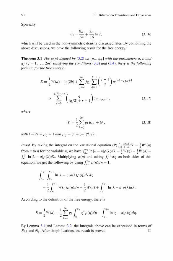
50 3 Bifurcation Transitions and Expansions
Specially
d1 = 9π
64+ 3π
16ln 2, (3.16)
which will be used in the non-symmetric density discussed later. By combining theabove discussions, we have the following result for the free energy.
Theorem 3.1 For ρ(η) defined by (3.2) on [η−, η+] with the parameters a, b andgj (j = 1, . . . ,2m) satisfying the conditions (3.3) and (3.4), there is the followingformula for the free energy:
E = 1
2W(a)− ln(2b)+
2m∑
j=2
jgj
j−1∑
q=1
(j − 1q
)
aj−1−qbq+1
×[q/2]−μq∑
r=0
(q
[q/2] + r + 1
)
Y2r+μq+1, (3.17)
where
Yl = 1
2
2m∑
k=0
gkRl,k +Θl, (3.18)
with l = 2r +μq + 1 and μq = (1 + (−1)q)/2.
Proof By taking the integral on the variational equation (P)∫Ω
ρ(λ)η−λ dλ = 1
2W′(η)
from a to η for the variable η, we have∫ η+η− ln |λ− η|ρ(λ)dλ= 1
2W(η)− 12W(a)+
∫ η+η− ln |λ − a|ρ(λ)dλ. Multiplying ρ(η) and taking
∫ η+η− dη on both sides of this
equation, we get the following by using∫ η+η− ρ(η)dη = 1,
∫ η+
η−
∫ η+
η−ln |λ− η|ρ(λ)ρ(η)dλdη
= 1
2
∫ η+
η−W(η)ρ(η)dη− 1
2W(a)+
∫ η+
η−ln |λ− a|ρ(λ)dλ.
According to the definition of the free energy, there is
E = 1
2W(a)+ 1
2
2m∑
k=0
gk
∫ η+
η−ηkρ(η)dη−
∫ η+
η−ln |η− a|ρ(η)dη.
By Lemma 3.1 and Lemma 3.2, the integrals above can be expressed in terms ofRl,k and Θl . After simplifications, the result is proved. �
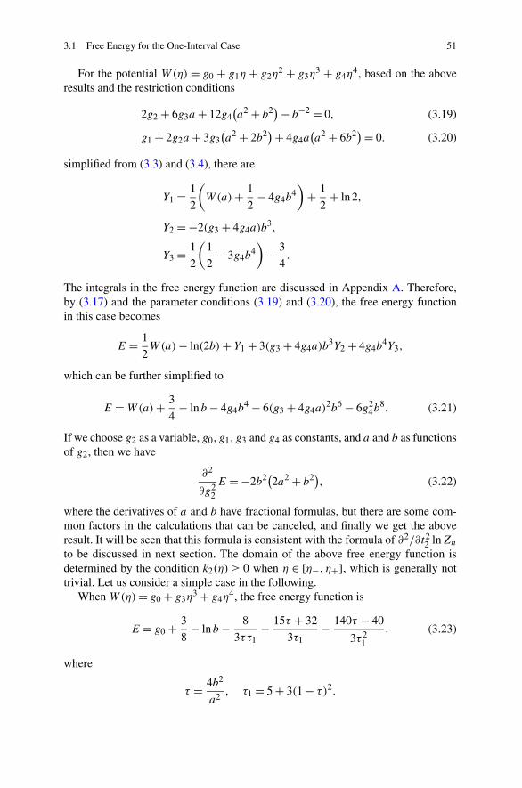
3.1 Free Energy for the One-Interval Case 51
For the potential W(η) = g0 + g1η + g2η2 + g3η
3 + g4η4, based on the above
results and the restriction conditions
2g2 + 6g3a + 12g4(a2 + b2)− b−2 = 0, (3.19)
g1 + 2g2a + 3g3(a2 + 2b2)+ 4g4a
(a2 + 6b2)= 0. (3.20)
simplified from (3.3) and (3.4), there are
Y1 = 1
2
(
W(a)+ 1
2− 4g4b
4)
+ 1
2+ ln 2,
Y2 = −2(g3 + 4g4a)b3,
Y3 = 1
2
(1
2− 3g4b
4)
− 3
4.
The integrals in the free energy function are discussed in Appendix A. Therefore,by (3.17) and the parameter conditions (3.19) and (3.20), the free energy functionin this case becomes
E = 1
2W(a)− ln(2b)+ Y1 + 3(g3 + 4g4a)b
3Y2 + 4g4b4Y3,
which can be further simplified to
E =W(a)+ 3
4− lnb− 4g4b
4 − 6(g3 + 4g4a)2b6 − 6g2
4b8. (3.21)
If we choose g2 as a variable, g0, g1, g3 and g4 as constants, and a and b as functionsof g2, then we have
∂2
∂g22
E = −2b2(2a2 + b2), (3.22)
where the derivatives of a and b have fractional formulas, but there are some com-mon factors in the calculations that can be canceled, and finally we get the aboveresult. It will be seen that this formula is consistent with the formula of ∂2/∂t22 lnZn
to be discussed in next section. The domain of the above free energy function isdetermined by the condition k2(η) ≥ 0 when η ∈ [η−, η+], which is generally nottrivial. Let us consider a simple case in the following.
When W(η)= g0 + g3η3 + g4η
4, the free energy function is
E = g0 + 3
8− lnb− 8
3ττ1− 15τ + 32
3τ1− 140τ − 40
3τ 21
, (3.23)
where
τ = 4b2
a2, τ1 = 5 + 3(1 − τ)2.

52 3 Bifurcation Transitions and Expansions
As discussed in Sect. 2.5, the parameter τ is restricted in the intervals (0, τ−] and[τ+,∞), where τ− ≈ 0.28 and τ+ ≈ 3.24.
When W(η)= g2η2 + g4η
4, the free energy becomes
E = g0 + 3
4− lnb+ 1
24
(2g2b
2 − 1)(
9 − 2g2b2), (3.24)
which agrees with the result
E(g)=E(0)+ 1
24
(b2 − 1
)(9 − b2)− 1
2lnb2. (3.25)
obtained in [3] for W(η)= 12η
2 + gη4. If we think E as a function of 2g2b2, it can
be seen that E has an extreme minimum point at 2g2b2 = 2, or at g4 = gc4, where
gc4 = − g22
12 , which is always not positive. For the non-symmetric density discussedabove, g4 is positive at such point.
If W(η) = g3η3 + g4η
4 is degenerated to W(η) = g4η4 by taking a → 0, the
free energy becomes E = 3/8 − lnb. It is the same result as W(η) = g2η2 + g4η
4
is degenerated to W(η)= g4η4. So the results obtained above are consistent. In this
chapter, we talk about the third-order phase transitions for the potential
W(η)= g1η+ g2η2 + g3η
3 + g4η4, (3.26)
caused by the bifurcation of the parameter(s) in the density models, or when thedensity on one-interval is split to a two-interval case, that will be discussed in thefollowing sections.
3.2 Partition Function and Toda Lattice
We have seen in last section that the free energy in the one-interval case can beexplicitly derived. For the multiple-interval cases, the free energy is expressed interms of elliptic integrals that are generally hard to be simplified. However, thederivatives of lnZn, which is how the free energy is defined, have some generalproperties that are useful to discuss the multiple-interval cases. In this section, weare going to discuss the derivatives of lnZn by using the equations obtained fromthe orthogonal polynomials for the potential
V (z)=4∑
j=0
tj zj , t4 > 0. (3.27)
Let us first consider the derivatives ∂uk/∂t1 for k = 0,1, . . . , n−1, where u0h0 =∫∞−∞ e−V (z)dz, and ∂vk/∂t1 for k = 1,2, . . . , n−1. Since h0 = ∫∞
−∞ e−V (z)dz, there

3.2 Partition Function and Toda Lattice 53
is ∂h0∂t1
= − ∫∞−∞ ze−V (z)dz = −u0h0, which implies ∂
∂t1lnh0 = −u0. When k ≥ 1,
hk = ∫∞−∞ p2
ke−V (z)dz, and
∂hk
∂t1= −
∫ ∞
−∞zp2
ke−V (z)dz= −ukhk.
Therefore, we have
∂
∂t1lnhk = −uk, (3.28)
for k ≥ 0. Since p0 = 1, zp0 = p1 + u0p0, p1 = z− u0, and p1,t1 = v1p0 obtainedfrom the orthogonality
∫∞−∞ p1,t1p0e
−V (z)dz= ∫∞−∞ p1,t1p0Vt1(z)e
−V (z)dz= v1h0,we have
∂u0
∂t1= −v1. (3.29)
When k ≥ 1, taking ∂/∂t1 on both sides of the recursion formula zpk = pk+1 +ukpk + vkpk−1 and applying the relation pk,t1 = vkpk−1, there is
∂uk
∂t1= vk − vk+1. (3.30)
In addition, since vk = hk/hk−1 for k ≥ 1, there is
∂vk
∂t1= vk
(∂ lnhk∂t1
− ∂ lnhk−1
∂t1
)
= vk(uk−1 − uk). (3.31)
The differential equations above and in the following for the uk and vk are generallycalled Toda lattice in the Hermitian matrix models. In the t1 direction, these equa-tions can be changed to the original Toda lattice for a chain of particles with nearestneighbor interaction by using the Flaschka’s variables. Since the partition function
Zn =∫ ∞
−∞· · ·∫ ∞
−∞e−Σn
i=1V (zi )∏
j<k
(zj − zk)2dz1 · · ·dzn
can be expressed as
Zn = n!h0h1 · · ·hn−1, (3.32)
we then get
∂
∂t1lnZn = −(u0 + · · · + un−1), (3.33)
and
∂2
∂t21
lnZn = vn. (3.34)

54 3 Bifurcation Transitions and Expansions
Next, let us consider the derivatives with respect to t2. According to (3.32), wefirst need ∂hk/∂t2 for k = 0,1, . . . , n− 1. Since h0 = − ∫∞
−∞ e−V (z)dz, there is
∂h0
∂t2= −
∫z2e−V (z)dz= −
∫(p1 − u0)
2e−V (z)dz= −(u20 + v1
)h0,
which implies
∂
∂t2lnh0 = −(u2
0 + v1). (3.35)
When k ≥ 1, there is
∂
∂t2lnhk = −(u2
k + vk + vk+1), (3.36)
by applying the recursion formula twice to ∂hk/∂t2 = − ∫ z2p2ke
−V (z)dz. Hence,we get
∂
∂t2lnZn = −(u2
0 + v1)−
n−1∑
k=1
(u2k + vk + vk+1
). (3.37)
To get the second-order derivative of lnZn, we need to consider the derivatives ofuk and vk . Since u0h0 = ∫ ze−V (z)dz, we can get ∂u0/∂t2 = −(u0 + u1)v1, andsimilarly
∂v1
∂t2= v1
(∂ lnh1
∂t2− ∂ lnh0
∂t2
)
= −v1(u2
1 − u20 + v2
).
Then, there is
∂
∂t2
(u2
0 + v1)= −v1
((u0 + u1)
2 + v2). (3.38)
When k ≥ 1, by ukhk = ∫ zp2ke
−V (z)dz we can get
∂uk
∂t2= −(uk+1 + uk)vk+1 + (uk + uk−1)vk. (3.39)
Similar to ∂v1/∂t2, there is
∂vk
∂t2= vk
(∂ lnhk∂t2
− ∂ lnhk−1
∂t2
)
= −vk(u2k − u2
k−1 + vk+1 − vk−1). (3.40)
When all the uk’s vanish in the even potential case, this equation becomes the equa-tion discussed by Fokas, Its and Kitaev in 1991. The following result is true fork ≥ 1,
∂
∂t2
(u2k +vk +vk+1
)= −vk+2vk+1 +vkvk−1 −vk+1(uk+1 +uk)2 +vk(uk +uk−1)
2.
(3.41)

3.3 Merged and Split Densities 55
By taking derivative with respect to t2 on both sides of (3.37), and applying theformulas (3.38) and (3.41) above, we get the following identity after canceling thelike terms,
∂2
∂t22
lnZn = vn((un + un−1)
2 + vn−1 + vn+1). (3.42)
We can also study the second-order derivatives in the t3 or t4 direction. It canbe found that the second-order derivatives have simple formulations in terms ofun’s and vn’s. As we have experienced and to be discussed later that the un and vnformulation for the second-order derivatives of lnZn always leads to the continuityof the second-order derivatives of the free energy. If the second-order derivative ofthe free energy has a singularity, then the center or radius parameter reduced fromun or vn also has singularity, and vice versa. These observations partially explain thecause of the third-order transitions we will discuss next by using the string equationand Toda lattice.
3.3 Merged and Split Densities
In this section, we discuss the properties of the densities on one or two intervalsto get ready for the analysis for the phase transition problems. In some literatures,the densities are classified as weak or strong densities. For a convenience of thegeometrical imagination, the densities discussed here are just called merged or splitdensity depending the parameters in the density is in the merged or split state. Also,we will explain that it is generally hard to have a explicit or simple formula for thefree energy function or the derivative the free energy to analyze the discontinuity atthe critical point since for the split density the free energy is generally expressed interms of the elliptic integrals, even in some special cases, like the symmetric caseto be discussed in Sect. 3.5, the free energy has a simple formula as the one-intervalcase given in Sect. 3.1. Therefore, the ε-expansion method discussed in Sect. 3.4would be generally applicable.
Let us consider the potential W(η) =∑4j=1 gjη
j and the densities discussed in
Chap. 1 on Ω1 = [η−, η+] and Ω2 = [η(1)− , η(1)+ ] ∪ [η(2)− , η
(2)+ ] on the real line. For
the purpose in this section, let us write the density on Ω1 in the following form,
ρ1(η)= 1
2π
(2g2 + 3g3(η+ a)+ 4g4
(η2 + aη+ a2 + 2b2))
√4b2 − (η− a)2,
(3.43)where η ∈ Ω1 = [a − 2b, a + 2b] and the parameters are restricted to satisfy thefollowing relations
2g2 + 6g3w1 + 12g4(w2
1 +w2)−w−1
2 = 0, (3.44)
g1 + 2g2w1 + 3g3(w2
1 + 2w2)+ 4g4w1
(w2
1 + 6w2)= 0, (3.45)

56 3 Bifurcation Transitions and Expansions
and
w1 = a, w2 = b2. (3.46)
For the density on Ω2, let us first write it in the following form,
ρ2(η) = 1
2π
(3g3 + 4g4(η+ a1 + a2)
)
× Re√e−πi[((η− a1)(η− a2)− b2
1 − b22
)2 − 4b21b
22
], (3.47)
subject to the following conditions
4g4w22 − 1 = 0, (3.48)
2g2 + (3g3 + 4g4w1)w1 − 4g4w3 = 0, (3.49)
g1 − (3g3 + 4g4w1)w3 = 0, (3.50)
where
w1 = (a1 + a2)/2, w2 = b1b2, w3 = a1a2 − b21 − b2
2. (3.51)
The wj parameters are introduced in an attempt to have a unified density formulafor the merged and split phases. The parameters of the polynomial in the square rootin (3.47) can be written in terms of the wj ’s according to the following factorization,
((η− a1)(η− a2)− b2
1 − b22
)2 − 4b21b
22
=[(
η− a1 + a2
2
)2
− 1
4(a1 − a2)
2 − (b1 − b2)2]
×[(
η− a1 + a2
2
)2
− 1
4(a1 − a2)
2 − (b1 + b2)2]
= [(η−w1)2 −w2
1 + 2w2 +w3][(η−w1)
2 −w21 − 2w2 +w3
]
= (η− η(1)−)(η− η
(1)+)(η− η
(2)−)(η− η
(2)+), η
(1)− < η
(1)+ < η
(2)− < η
(2)+ .
(3.52)
The real part of the square root in (3.47) takes a negative sign when η ∈ [η(1)− , η(1)+ ],
and it takes a positive sign when η ∈ [η(2)− , η(2)+ ]. In fact, if we denote Q(η)= (η−
η(1)− )(η− η
(1)+ )(η− η
(2)− )(η− η
(2)− ), then
√e−πiQ(η)=
{|√Q(η)|eπi, η
(1)− < η < η
(1)+ ,
|√Q(η)|, η(2)− < η < η
(2)+ ,
(3.53)
obtained according to the following argument values that if η ∈ (η(1)− , η
(1)+ ), then
arg(η−η(1)− )= 0, and arg(η−η′)= π for η′ = η
(1)+ , η
(2)− , η
(2)+ ; and if η ∈ (η
(2)− , η
(2)+ ),

3.3 Merged and Split Densities 57
there are arg(η− η′)= 0 for η′ = η(1)− , η
(1)+ , η
(2)− , and arg(η− η
(2)+ )= π . Therefore,
we also need 3g3 + 4g4(η+ a1 + a2)≤ 0 when η ∈ [η(1)− , η(1)+ ], and 3g3 + 4g4(η+
a1 + a2)≥ 0 when η ∈ [η(2)− , η(2)+ ] such that ρ2 keeps non-negative on Ω2.
When a1 = a2 = a = ac and b1 = b2 = b = bc for the fixed constants ac andbc > 0, both of the density functions above are degenerated to
ρc(η)= 1
π2gc4(η− ac)
2√
4b2c − (η− ac)2, η ∈ [ac − 2bc, ac + 2bc], (3.54)
at the critical point, and the parameters should take the values satisfying the follow-ing relations
4gc4b4c = 1, (3.55)
gc3 + 4gc4ac = 0, (3.56)
gc2 + 3gc3ac + 2gc4(3a2
c + 2b2c
)= 0, (3.57)
gc1 − (3gc3 + 8gc4ac)(a2c − 2b2
c
)= 0, (3.58)
or equivalently
gc1 = ac(2b2
c − a2c
)b−4c , 2gc2 = (3a2
c − 2b2c
)b−4,
3gc3 = −3acb−4c , 4gc4 = b−4
c .(3.59)
Here, the relation (3.56) is obtained based on the non-negative requirement for ρ1and ρ2 as discussed above.
One can image that it is hard to get the explicit formulas of the free energy func-tion for the density ρ2. If we consider the difference of the derivatives of the freeenergy for ρ1 and ρ2 at the critical point, the computations may be easier sincethe densities have a unified structure that many common terms could be canceledto simplify the calculations. In the following, let us discuss whether this strategyworks.
Recall that the density ρ1 on Ω1 = [η−, η+] = [a− 2b, a+ 2b] can be written asρ1 = 1
π
√detA(1) as shown in Chap. 1, where
A(1) = c1J(1) + c2
(J (1)
)2 + c3(J (1)
)3 − 1
2W ′(η)I, (3.60)
with c1 = 2g2 +6g3a+12g4(a2 +b2), c2 = 3g3 +12g4a, c3 = 4g4, I is the identity
matrix, and
J (1) =(
0 1−b2 η− a
)
. (3.61)
The density ρ2 can be changed to ρ2 = 1π
√detA(2), where
A(2) = (3g3 + 4g4(η+ a1 + a2))J (2) − 1
2W ′(η)I, (3.62)

58 3 Bifurcation Transitions and Expansions
with
J (2) =(
0 1−b2
1 η− a1
)(0 1
−b22 η− a2
)
. (3.63)
Further, we have
A(1) = B(1)(J (1))2 − 1
2W ′(η)I, and A(2) = B(2)J (2) − 1
2W ′(η)I, (3.64)
where
B(1) = (3g3 + 4g4(η+ 2a))I + (b−4 − 4g4
)(η− a −1b2 0
)
,
and
B(2) = (3g3 + 4g4(η+ a1 + a2))I.
If we define
Q(η)= 1
4
(W ′)2 −w2
2
(3g3 + 4g4(η+ 2w1)
)2
− (3g3 + 4g4(η+ 2w1))(
1 − 4g4w22
)(η−w1)−w−1
2
(1 − 4g4w
22
)2,
(3.65)
for η ∈ C, then
−detA(1) =Q|ρ1 and − detA(2) =Q|ρ2 , (3.66)
since 1 − 4g4w22 = 0 for ρ2, where Q|ρj means the parameters in Q are restricted
by the parameter conditions for ρj , j = 1,2.Let us consider the continuity or discontinuity of the derivatives of the free energy
function as the density is changed from ρ1 to ρ2. First, there is
∂√Q
∂g
∣∣∣∣ρj
= 〈Qw,w′〉 + 〈Qg,g′〉2√Q
∣∣∣∣ρj
, j = 1,2,
where w = (w1,w2,w3), g = (g1, g2, g3, g4), Qw and Qg are the gradients, ′ =∂/∂g and g is one of the gj ’s. It follows that
∂√Q
∂g
∣∣∣∣ρ1,g=gc
− ∂√Q
∂g
∣∣∣∣ρ2,g=gc
= 〈Qw,w′〉2√Q
∣∣∣∣ρ1,g=gc
− 〈Qw,w′〉2√Q
∣∣∣∣ρ2,g=gc
,
that implies the first-order derivative of the free energy is continuous at g = gc by thedirect calculations from the free energy formula. For the second-order derivatives,we can get
∂2
∂g2E(ρ1)
∣∣∣∣g=gc
− ∂2
∂g2E(ρ2)
∣∣∣∣g=gc
= −1
2πi
∮∂W(η)
∂g
〈Qcw,w(1) − w(2)〉
2√Qc
dη,

3.4 Third-Order Phase Transition by the ε-Expansion 59
where Qc = Q|g=gc , and w(1) and w(2) are the corresponding vectors followingthe discussion above. It can be obtained that the second-order derivative is alsocontinuous at the critical point.
However, for the higher order derivatives this method will lead to complicatedcalculations. So the analysis for the phase transition will not be easy if one hopes touse the explicit formulas in such a way to get the discontinuity. Similar complexitieshave been experienced in other researches, for example, see [1, 12, 20]. In the nextsection, we discuss a different method to simplify the calculations for analyzing thenonlinear properties in the transitions.
3.4 Third-Order Phase Transition by the ε-Expansion
After we have experienced the different strategies or properties in the previous sec-tions, let us talk about the ε-expansion method. We will see that the ε-expansionsfor the parameters based on the algebraic equations reduced from the string equationcan quickly give the phase transition properties including the critical phenomena tobe discussed in the later chapters.
Consider the Hermitian matrix model with the potential W(η) = ∑4j=1 gjη
j .The phase transition problem is to discuss whether a derivative of the free energyfunction
E =∫
Ω
W(η)ρ(η)dη−∫
Ω
∫
Ω
ln |λ− η|ρ(λ)ρ(η)dλdη (3.67)
becomes discontinuous as the density ρ is changed from one to another, for example,from ρ1 to ρ2. In the following, we will discuss that the discontinuity is mainlycaused by the change of the parameter conditions.
Rewrite (3.47) as
ρ2(η)= 1
2π
(3g3 + 4g4(η+ 2u)
)Re√e−πi[(η− u)2 − x2
1
][(η− u)2 − x2
2
],
(3.68)for η ∈Ω2 = [u− x2, u− x1] ∪ [u+ x1, u+ x2], where
x21 = u2 −w− 2v = 1
4(a1 − a2)
2 + (b1 − b2)2, (3.69)
x22 = u2 −w+ 2v = 1
4(a1 − a2)
2 + (b1 + b2)2 (3.70)
and
u= (a1 + a2)/2, v = b1b2, w = a1a2 − b21 − b2
2. (3.71)
Denote
ω2(η)= 1
2
(3g3 + 4g4(η+ 2u)
)√[(η− u)2 − x2
1
][(η− u)2 − x2
2
], (3.72)
for η in the complex plane outside Ω2.

60 3 Bifurcation Transitions and Expansions
Fig. 3.1 Contours for thesecond formula in (3.73)
For the models considered in this book, we can discuss the first-order derivativeas follows. Consider the following formulas for the density ρ2,
{(P)∫Ω2
ρ2(λ)η−λ dλ= 1
2W′(η), η ∈ (η
(1)− , η
(1)+ )∪ (η
(2)− , η
(2)+ ),
∫Ω2
ρ2(λ)η−λ dλ= 1
2W′(η)−ω2(η), η ∈ (η
(1)+ , η
(2)− ).
(3.73)
The first formula above is the variational equation for the eigenvalue density. Thesecond formula is, in fact, true for any η outside the cuts. For the discussion ofthe free energy, we specially pay attention to η ∈ (η
(1)+ , η
(2)− ). To prove the second
formula, consider the counterclockwise contours Ω∗2 around the cuts Ω2 and the
counterclockwise circle γ ∗η around a point η in the complex plane, see Fig. 3.1.
By Cauchy theorem, there is
1
2πi
∫
Ω∗2 ∪γ ∗
η
ω2(λ)
λ− ηdλ= 1
2πi
∫
|λ|=Rω2(λ)
λ− ηdλ,
where R is a large number, and the right hand side is equal to 12W
′(η) as we havediscussed before. For the left hand side, there is
1
2πi
∫
Ω∗2
ω2(λ)
λ− ηdλ+ 1
2πi
∫
γ ∗η
ω2(λ)
λ− ηdλ=
∫
Ω2
ρ2(λ)
η− λdλ+ω2(η),
which shows the second formula above. Note that the point η can be large in thecomplex plane. The formula ω2(η)= 1
2W′(η)+∫
Ω2
ρ2(λ)λ−η dλ can be connected to the
asymptotics ω2(η) = 12W
′(η)− η−1 +O(η−2) as η → ∞. In fact, when η → ∞,∫Ω2
ρ2(λ)λ−η dλ collects all the rest terms in the expansion of ω2 after the leading term
12W
′(η).Now, by the free energy formula (3.67) there is
∂
∂gE(ρ2) =
∫
Ω2
∂W(η)
∂gρ2(η)dη
− 2
(∫ η(1)+
η(1)−
+∫ η
(2)+
η(2)−
)(∫
Ω2
ln |η− λ|ρ2(λ)dλ− 1
2W(η)
)∂ρ2(η)
∂gdη,
(3.74)

3.4 Third-Order Phase Transition by the ε-Expansion 61
where g represents any one of the gj ’s. We can get that for η ∈ (η(1)− , η
(1)+ ), there is
∫
Ω2
ln |η− λ|ρ2(λ)dλ− 1
2W(η)=
∫
Ω2
ln |η(1)− − λ|ρ2(λ)dλ− 1
2W(η(1)−), (3.75)
and for η ∈ (η(2)− , η
(2)+ ), there is
∫
Ω2
ln |η− λ|ρ2(λ)dλ− 1
2W(η)
=∫
Ω2
ln |η(1)− − λ|ρ2(λ)dλ− 1
2W(η(1)−)−∫ η
(2)−
η(1)+
ω2(η)dη. (3.76)
Consequently, by using∫Ω2
∂∂gρ2(η)dη = ∂
∂g
∫Ω2
ρ2(η)dη = 0 there is the followingresult since ρ2 is equal to 0 at the end points of Ω2.
Theorem 3.2 For the free energy function (3.67), we have
∂
∂gE(ρ)=
⎧⎨
⎩
∫Ω1
∂W(η)∂g
ρ1(η)dη, ρ = ρ1,
∫Ω2
∂W(η)∂g
ρ2(η)dη+ 2∫ η(2)−η(1)+
ω2(η)dη∂∂g
∫ η(2)+η(2)−
ρ2(η)dη, ρ = ρ2,
(3.77)where g is one of the gj ’s.
However, the higher order derivatives of the free energy will involve the ellipticintegral calculations. It is experienced [1, 9, 12, 20] that the elliptic integral calcu-lations are complicated. We have also discussed in last section that the algebraicmethod does not help too much to get a simple result for the free energy on theentire domain of the parameters. For the transition problems, it would be easier tojust work on the behaviors around the critical point. The algebraic equations for theparameters obtained from the string equation can give the behaviors on both sidesof the critical point by the ε-expansions. Also, when the degree of the potentialis higher, the elliptic integrals will become more complicated, but the expansionmethod still works for the models of higher degree potentials to get at least thebehaviors at the critical point(s) for analyzing the continuity or discontinuity.
Let us first consider the parameters in ρ2. Applying the notations u = (a1 +a2)/2, v = b1b2 and w = a1a2 − b2
1 − b22 into (3.48), (3.49) and (3.50). we see that
(3.49) and (3.50) become
2g2 + 6g3u+ 12g4(4u2 −w
)= 0, (3.78)
g1 − (3g3 + 8g4u)w = 0. (3.79)
Since the above equations do not involve v, let us expand u and w in terms ofε1 = g2 − gc2,
u= uc(1 + α1ε1 + α2ε
21 + α3ε
31 + · · · ), (3.80)
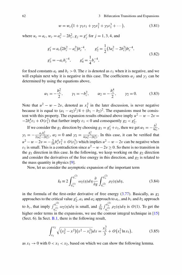
62 3 Bifurcation Transitions and Expansions
w =wc
(1 + γ1ε1 + γ2ε
21 + γ3ε
31 + · · · ), (3.81)
where uc = ac , wc = a2c − 2b2
c , gj = gcj for j = 1,3,4, and
gc1 = ac(2b2
c − a2c
)b−4c , gc2 = 1
2
(3a2
c − 2b2c
)b−4c ,
gc3 = −acb−4c , gc4 = 1
4b−4c ,
(3.82)
for fixed constants ac and bc > 0. The ε is denoted as ε1 when it is negative, and wewill explain next why it is negative in this case. The coefficients αj and γj can bedetermined by using the equations above,
α1 = −b2c
2, γ1 = −b2
c , α2 = −b4c
2, γ2 = 0. (3.83)
Note that u2 − w − 2v, denoted as x21 in the later discussion, is never negative
because it is equal to (a1 − a2)2/4 + (b1 − b2)
2. The expansions must be consis-tent with this property. The expansion results obtained above imply u2 −w− 2v =−2b4
cε1 +O(ε21) that further imply ε1 < 0 and consequently g2 < gc2.
If we consider the g1 direction by choosing g1 = gc1 +ε1, then we get α1 = − b2c
4ac,
γ1 = − acb2c
2(a2c−2b2
c ), α2 = 0 and γ2 = b3
c
4(a2c−2b2
c ). In this case, it can be verified that
u2 −w− 2v = − 316b
4cε
21 +O(ε3
1) which implies u2 −w− 2v can be negative whenε1 is small. This is a contradiction since u2 −w−2v ≥ 0. So there is no transition inthe g1 direction in this case. In the following, we keep working on the g2 directionand consider the derivatives of the free energy in this direction, and g2 is related tothe mass quantity in physics [9].
Now, let us consider the asymptotic expansion of the important term
I0 ≡ 2∫ η
(2)−
η(1)+
ω2(η)dη∂
∂g
∫ η(2)+
η(2)−
ρ2(η)dη, (3.84)
in the formula of the first-order derivative of free energy (3.77). Basically, as g2
approaches to the critical value gc2, a1 and a2 approach to ac , and b1 and b2 approach
to bc, that imply∫ η(2)−η(1)+
ω2(η)dη is small, and ∂∂g
∫ η(2)+η(2)−
ρ2(η)dη is O(1). To get the
higher order terms in the expansions, we use the contour integral technique in [15](Sect. 6). In Sect. B.1, there is the following result,
∫ x2
x1
√(x2
2 − x2)(x2 − x2
1
)dx = x3
2
3+O
(x2
1 lnx1), (3.85)
as x1 → 0 with 0 < x1 < x2, based on which we can show the following lemma.

3.4 Third-Order Phase Transition by the ε-Expansion 63
Lemma 3.4 For ρ2 defined by (3.47), there is
∫ η(2)+
η(2)−
ρ2(η)dη = 1
2− 2
πacbcε1 +O
(ε2
1 ln |ε1|), (3.86)
as ε1 → 0, where g2 = gc2 + ε1 and ε1 < 0.
Proof First, we have
∫ η(2)+
η(2)−
ρ2(η)dη = 1
2π
∫ η(2)+
η(2)−
(3g3 + 4g4(η+ a1 + a2)
)√(2v −Λ)(Λ+ 2v)dη,
where v = b1b2 and Λ= (η− a1)(η− a2)− b21 − b2
2. Then,∫ η(2)+η(2)−
ρ2(η)dη is equal
to
g4
π
∫ x22
x21
√(x2
2 − ζ)(ζ − x2
1
)dζ + 1
2π(3g3 + 12g4u)
∫ x2
x1
√(x2
2 − x2)(x2 − x2
1
)dx,
where ζ = (η − u)2, x = η − u and u = (a1 + a2)/2 given above. We then obtain
the following since∫ x2
2
x21
√(x2
2 − ζ )(ζ − x21)dζ = 2πv2,
∫ η(2)+
η(2)−
ρ2(η)dη = 2g4v2 + 1
2π(3g3 + 12g4u)
∫ x2
x1
√(x2
2 − x2)(x2 − x2
1
)dx.
By the formula (3.85), we further have
∫ η(2)+
η(2)−
ρ2(η)dη = 2g4b4c + 1
2π(3g3 + 12g4u)
x32
3+O
((3g3 + 12g4u)x
21 lnx1
).
Since 4g4b4c = 1, 3g3 + 12g4u= 12g4acα1ε1 +O(ε2
1), x21 =O(ε1) and x2 = 2bc +
O(ε1), the above expansion becomes
∫ η(2)+
η(2)−
ρ2(η)dη = 1
2− 2
πacbcε1 +O
(ε2
1 ln |ε1|).
Then the lemma is proved. �
Lemma 3.5∫ η
(2)−
η(1)+
ω2(η)dη = 3π
2acb
3cε
21 +O
(ε3
1
), (3.87)
as ε1 → 0, where ε1 = g2 − gc2 < 0.

64 3 Bifurcation Transitions and Expansions
Proof The formula
∫ η(2)−
η(1)+
ω2(η)dη = 1
2
∫ η(2)−
η(1)+
(3g3 + 4g4(η+ a1 + a2)
)√(Λ− 2v)(Λ+ 2v)dη,
can be changed to
∫ η(2)−
η(1)+
ω2(η)dη = 2g4
∫ u+x1
u−x1
(η− u)
√(x2
2 − (η− u)2)(x2
1 − (η− u)2)dη
+ 1
2(3g3 + 12g4u)
∫ x1
−x1
√(x2
2 − x2)(x2 − x2
1
)dx,
where x21 = u2 − w − 2v, x2
2 = u2 − w + 2v, and x = η − u. It is easy to see
that∫ x1−x1
t
√(x2
2 − t2)(x21 − t2)dt = 0 by the symmetry, that implies the first integral
on the right hand side is equal to 0. Note that the integral here is from −x1 tox1, that is different from the integral in the normalization of the density. For thesecond integral, we first have the expansion 3g3 + 12g4u= 12g4acα2ε1 +O(ε2
1)=− 3
2acb−2c ε1 +O(ε2
1). Then it follows that
∫ η(2)−
η(1)+
ω2(η)dη = −3
4acb
−2c ε1
∫ x1
−x1
√(x2
2 − x2)(x2 − x2
1
)dx +O
(ε3
1
).
Since x2 = 2bc +O(ε1) and x21 = −2b4
cε1 +O(ε21), where ε1 < 0, we have
∫ x1
−x1
√(x2
2 − x2)(x2 − x2
1
)dx = π
2x2x
21 +O
(ε2
1
)= −2b5cε1 +O
(ε2
1
).
Therefore, we finally get
∫ η(2)−
η(1)+
ω2(η)dη = 3π
2acb
3cε
21 +O
(ε3
1
),
and the lemma is proved. �
By the lemmas above and (3.84), we have the following.
Lemma 3.6
I0 = −6a2c b
4cε
21 +O
(ε3
1 ln |ε1|), (3.88)
as ε1 → 0, where ε1 = g2 − gc2 < 0.
The remaining work to find the expansion for
∂E(ρ2)
∂g2=∫
Ω2
η2ρ2dη+ I0

3.4 Third-Order Phase Transition by the ε-Expansion 65
is the ε-expansion for∫Ω2
η2ρ2dη. By the asymptotic expansion of ω2 = 12 (3g3 +
4g4(η+ 2u))(Λ2 − 4v2)1/2 as η → ∞, we can get that the coefficient of the η−3 is−[6g3u+ 4g4(8u2 −w)]v2, which implies
∫
Ω2
η2ρ2dη= −1
2πi
∫
|η|=Rη2ω2dη= [6g3u+ 4g4
(8u2 −w
)]v2.
Since we discuss the changes in the g2 direction by keeping other gj ’s to theircritical values and 4g4v
2 = 1, we have that v is constant when g2 < gc2 for the ρ2phase. Then, the ε1 expansions for u and w obtained above imply∫
Ω2
η2ρ2dη = a2c + 2b2
c − (4a2c + 2b2
c
)b2cε1 − 3a2
c b4cε
21 +O
(ε3
1 ln |ε1|). (3.89)
Combining the discussions above, we finally get the following result for the freeenergy for the ρ2 as g2 approaches to gc2 from the left.
Theorem 3.3 For the ρ2 defined by (3.47), there is
∂E(ρ2)
∂g2= a2
c + 2b2c − (4a2
c + 2b2c
)b2cε1 − 9a2
c b4cε
21 +O
(ε3
1 ln |ε1|), (3.90)
as ε1 → 0, where ε1 = g2 − gc2 < 0.
Now, let us consider the free energy for the density ρ1. By the asymptotic expan-sion of ω1(η) defined by
ω1(η)= 1
2
(2g2 + 3g3(η+ a)+ 4g4
(η2 + aη+ a2 + 2b2))((η− a)2 − 4b2)1/2
,
(3.91)as η → ∞ for η /∈Ω1 = [a − 2b, a + 2b], we can obtain that
∂E(ρ1)
∂g2=∫
Ω1
η2ρ1dη= −1
2πi
∫
|η|=Rη2ω1dη
= u2 + v + 6g3uv2 + 4g4
(6u2v2 + v3),
where u= a and v = b2. According to (3.19) and (3.20), the parameters satisfy
2g2 + 6g3u+ 12g4(u2 + v
)− v−1 = 0,
g1 + 2g2u+ 3g3(u2 + 2v
)+ 4g4u(u2 + 6v
)= 0.
To get the concrete value of the derivative at the critical point, consider the expan-sions
u= ac(1 + α1ε+ α2ε
2 + · · · ), (3.92)
v = b2c
(1 + β1ε+ β2ε
2 + · · · ), (3.93)
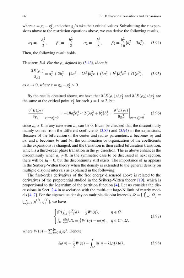
66 3 Bifurcation Transitions and Expansions
where ε = g2 −gc2, and other gj ’s take their critical values. Substituting the ε expan-sions above to the restriction equations above, we can derive the following results,
α1 = −b2c
2, β1 = −b2
c
2, α2 = −b4
c
8, β2 = b2
c
16
(b2c − 3a2
c
). (3.94)
Then, the following result holds.
Theorem 3.4 For the ρ1 defined by (3.43), there is
∂E(ρ1)
∂g2= a2
c + 2b2c − (4a2
c + 2b2c
)b2cε+ (3a2
c + b2c
)b4cε
2 +O(ε3), (3.95)
as ε → 0, where ε = g2 − gc2 > 0.
By the results obtained above, we have that ∂jE(ρ1)/∂gj
2 and ∂jE(ρ2)/∂gj
2 arethe same at the critical point gc2 for each j = 1 or 2, but
∂3E(ρ2)
∂g32
∣∣∣∣g2→gc2−0
= −18a2c b
4c < 2
(3a2
c + b2c
)b4c = ∂3E(ρ1)
∂g32
∣∣∣∣g2→gc2+0
, (3.96)
since bc > 0 in any case even ac can be 0. It can be checked that the discontinuitymainly comes from the different coefficients (3.83) and (3.94) in the expansions.Because of the bifurcation of the center and radius parameters, a becomes a1 anda2, and b becomes b1 and b2, the combination or organization of the coefficientsin the expansions is changed, and the transition is then called bifurcation transition,which is a third-order phase transition in the g2 direction. The I0 above enhances thediscontinuity when ac = 0. In the symmetric case to be discussed in next section,there will be I0 = 0, but the discontinuity still exists. The importance of I0 appearsin the Seiberg-Witten theory when the density is extended to the general density onmultiple disjoint intervals as explained in the following.
The first-order derivatives of the free energy discussed above is related to thederivatives of the prepotential studied in the Seiberg-Witten theory [19], which isproportional to the logarithm of the partition function [4]. Let us consider the dis-cussions in Sect. 2.4 in association with the multi-cut large-N limit of matrix mod-els [4, 7]. For the eigenvalue density on multiple disjoint intervals Ω =⋃l
j=1Ωj ≡⋃l
j=1[η(j)− , η(j)+ ], we have
⎧⎨
⎩
(P)∫Ω
ρ(λ)η−λ dλ= 1
2W′(η), η ∈Ω,
∫Ω
ρ(λ)η−λ dλ= 1
2W′(η)−ω(η), η ∈C�Ω,
(3.97)
where W(η)=∑2mj=0 gjη
j . Denote
S0(η)= 1
2W(η)−
∫
Ω
ln |η− λ|ρ(λ)dλ, (3.98)

3.4 Third-Order Phase Transition by the ε-Expansion 67
for η in the complex plane. By (3.97), for a point η in (η(j)− , η(j)+ ), there is S0(η)=
S0(η(1)− ) +∑j−1
k=1
∫Ωk
ω(η)dη, where Ω =⋃l−1k=1 Ωk ≡⋃l−1
k=1(η(k)+ , η
(k+1)− ). And if
η ∈ (η(j)+ , η
(j+1)− ), then there is S0(η) = S0(η
(1)− ) + Re
∫ ηη(1)−ω(λ)dλ. Since ω(η) is
real on Ω and imaginary on Ω , there is the following general formula
S0(η)= S0(η(1)−)+ Re
∫ η
η(1)−ω(λ)dλ, (3.99)
or dS0(η)= Reω(η)dη in the differential form. It can be seen that if η ∈Ω , then
∂S0(η)
∂η= 0, (3.100)
since Reω(η) = 0 on the cuts Ω . The function S0(η) is then a step function onΩ ∪ Ω , as discussed in the Seiberg-Witten theory, for example, see [4, 10]. Thedifferential dS(η)= ω(η)dη for η ∈ C�Ω is corresponding to the Seiberg-Wittendifferential or the extended differentials defined on the Riemann surface, and freeenergy E is proportional to the prepotential.
Since the derivative of the free energy with respect to a potential direction g canbe represented as
∂
∂gE =
∫
Ω
∂W(η)
∂gρ(η)dη+ 2
∫
Ω
S0(η)∂ρ(η)
∂gdη, (3.101)
as shown before, it is then equal to∫
Ω
∂W(η)
∂gρ(η)dη+ 2S0
(η(1)−)∫
Ω
∂ρ(η)
∂gdη+ 2 Re
∫
Ω
(∫ η
η(1)−ω(λ)
∂ρ(η)
∂gdλ
)
dη.
(3.102)After simplifications, there is
∂
∂gE =
∫
Ω
∂W(η)
∂gρ(η)dη+ 2
l∑
j=2
j−1∑
k=1
∫
Ωk
ω(λ)dλ∂
∂g
∫
Ωj
ρ(η)dη, (3.103)
which is consistent to the result (3.77) for the two-cut case (l = 2).The Seiberg-Witten theory is developed to study the mass gap problem in the
quantum Yang-Mills theory [11]. The linear combination of a and aD [4, 10, 19],which are the integrals of the Seiberg-Witten differential over different intervals, isused to define the mass quantity according to the physical literatures. The connec-tion between the Seiberg-Witten differential and the eigenvalue density in matrixmodels is important, that involves complicated mathematical and physical prob-lems. A simple linear combination example of the integrals of the ρ and ω overdifferent intervals is discussed in Sect. B.2 in order to experience the mathematicalproperties, and it is seen that the integrals are related to the Legendre’s relation inthe elliptic integral theory.

68 3 Bifurcation Transitions and Expansions
The relevant researches, such as instanton, integrable systems, string theory, su-persymmetric Yang-Mills theory and Whitham equations can be found, for example,in [2, 5–7, 14, 17, 18] and the references therein. There are also other methods toinvestigate the mass gap problem, including, for example, Euler-Lagrange equation,energy-momentum operator, renormalization, propagator and much more that canbe found in the publications and the archive journals. There are many challengingproblems in this field, and one important problem related to our discussion is tobalance the finite freedoms and the integrability. In the position models such as thesoliton integrable systems with infinitely many constants, it is usually complicatedto reduce the infinite dimensional space by using the periodic conditions as studiedin the quantum inverse scattering method [13]. In the momentum aspect, the inte-grable system characterized by the infinitely many functions such as the un and vncan be reduced to the physical model with finite number of parameters such as theaj and bj satisfying certain conditions, and the degree of the potential polynomialdetermines the degree of the freedoms.
The string equations are related to the density problems in the Seiberg-Wittentheory as explained above. But the entire story would be complicated. As MichaelR. Douglas mentioned in 2004 [8], it remains a fertile ground for mathematicaldiscovery. There is a large field behind this fundamental problem that will connectmany different researches and motivate the developments of sciences. Uncertaintyand Fourier transform are fundamental in this research area, that have been typicallyemphasized in [11], and are associated with diverse problems.
3.5 Symmetric Cases
On the real line, denote Ω1 = [−η1, η1] and Ω2 = [−η2,−η0] ∪ [η0, η2], and con-sider the potential W(η)= g2η
2 + g4η4, where g4 > 0. The densities on Ω1 and Ω2
are all symmetric now.According to the discussion in last section, the density on Ω1 now becomes
ρ1(η)= 1
π
(g2 + g4
(2η2 + η2
1
))√η2
1 − η2, η ∈Ω1, (3.104)
where η1 = 2b, and the parameters satisfy the following conditions
g2 + 4g4b2 ≥ 0, (3.105)
2g2b2 + 12g4b
4 = 1. (3.106)
It is easy to see that (3.105) implies ρ1(η) ≥ 0 for η ∈ Ω1. The conditions (3.105)and (3.106) imply g2b
2 + 1 = 3(g2 + 4g4b2)b2 ≥ 0, or −g2 ≤ 1/b2. When g2 is
negative, there is (−g2)2 ≤ (1/b2)(4g4b
2)= 4g4, or
g2 ≥ −2√g4. (3.107)

3.5 Symmetric Cases 69
When g2 is positive, (3.107) is also true. So (3.107) defines the region of the pa-rameters for ρ1, and the parameters for ρ2 will stay in the region g2 ≤ −2
√g4.
As a remark, the ρ1 is an extension of the planar diagram density [3] ρ(η) =1π( 1
2 + 4gb2 + 2gη2)√
4b2 − η2 for potential W(η)= 12η
2 + g4η4 since the g2 con-
sidered here is negative around the critical point. The parameter g4 in [3] is negativeas they discuss the singular point for the free energy. Here, we consider positive g4.The critical point g2/
√g4 = −2 was found early in 1982 by Shimamune [20], and
the relevant discussions about the phase transition can also be found in [1, 9, 12],for instance.
The densities given above satisfy the normalization and the variational equationas shown before. It has been discussed in Sect. 3.1 that the free energy can be cal-culated by using the analytic function
ω1(η)= (g2 + g4(2η2 + η2
1
))√η2 − η2
1, η ∈ C�Ω1, (3.108)
which has the following asymptotics
ω1(η)= 1
2
(2g2η
2 + 4g4η3)− (g2 + 6g4b
2)2b2
η− (g2 + 8g4b
2)2b4
η3+O
(1
η5
)
,
(3.109)as η → ∞ in the complex plane.
Now, let us consider
ρ2(η)= 2g4
πηRe
√e−πi(η2 − η2
0
)(η2 − η2
2
), η ∈Ω2 = [−η2,−η0] ∪ [η0, η2],
(3.110)where η0 = b2 − b1, η2 = b1 + b2, and the parameters satisfy
4g4b21b
22 = 1, (3.111)
g2 + 2g4(b2
1 + b22
)= 0, (3.112)
which imply
g2 = −2g4(b2
1 + b22
)≤ −4g4b1b2 = −2√g4. (3.113)
Therefore, the regions of the parameters in densities (3.104) and (3.110) are sepa-rated by the curve
g2 = −2√g4, (3.114)
in the (g2, g4) plane. The ρ1 is defined when g2 ≥ −2√g4, and ρ2 is defined when
g2 ≤ −2√g4. In addition, since
√(η2 − η2
0
)(η2 − η2
2
)=⎧⎨
⎩
|√(η2 − η2
0)(η2 − η2
2)|e3πi/2, −η2 < η <−η0,
|√(η2 − η2
0)(η2 − η2
2)|eπi/2, η0 < η < η2,
(3.115)

70 3 Bifurcation Transitions and Expansions
there is ρ2(η) > 0 when η ∈ (−η2,−η0) ∪ (η0, η2). In fact, if η ∈ (−η2,−η0).there are arg(η − (−η2)) = 0, and arg(η − η′) = π for η′ = −η0, η0, η2; and ifη ∈ (η0, η2), there are arg(η− η′)= 0 for η′ = −η2,−η0, η0, and arg(η− η2)= π .
Define another analytic function
ω2(η)= 2g4η
√(η2 − η2
0
)(η2 − η2
2
), η ∈ C�Ω2, (3.116)
which has the asymptotics
ω2(η)= 1
2
(2η+ 4g4η
3)− 4g4b21b
22
η+O
(η−3), (3.117)
as η → ∞ in the complex plane. It can be checked that if b1 = b2 = b, then η0 = 0and η1 = η2, and the conditions (3.111) and (3.112) become 4g4b
4 = 1 and g2 +4g4b
2 = 0 respectively, which imply (3.106). In other words, (3.111) and (3.112)can be thought as (3.106) is split to two equations as b is bifurcated to the twoparameters b1 and b2. In the symmetric cases, we can experience the third-orderphase transitions with the explicit formulations of the free energy function.
To calculate the free energy function, let us make a change for ρ2 by the following
ρ2(η)dη = 1
2ρ2(ζ )dζ, (3.118)
where
ρ2(ζ )= 2g4
π
√(ζ+ − ζ )(ζ − ζ−), (3.119)
ζ− = η20, ζ+ = η2
2, ζ = η2, and W(η) = 12W (ζ ) with W (ζ ) = 2g2ζ + 2g4ζ
2 such
that η−1∂W(η)/∂η = ∂W (ζ )/∂ζ . The coefficients 1/2 and 2 above will make thefollowing calculations easy. Since ρ2(η) satisfies
∫ −η0−η2
ρ2(η)dη+ ∫ η2η0ρ2(η)dη = 1,
and
(P)∫ −η0
−η2
ρ2(λ′)
η− λ′ dλ′ + (P)
∫ η2
η0
ρ2(λ)
η− λdλ= 1
2W ′(η),
where ′ for W(η) means ∂/∂η, we can get∫ ζ+ζ− ρ2(ζ )dζ = 1, and
(P)∫ ζ+
ζ−
ρ2(ξ)
ζ − ξdξ = 1
2W ′(ζ ), (3.120)
by taking λ′ = −λ, ξ = λ2 and ζ = η2, where ′ for W (ζ ) means ∂/∂ζ . Then, thefree energy becomes
E = 1
2
(
W (a)+ 3
4− ln b
)
, (3.121)
by using the free energy for the one-interval case discussed in Sect. 3.1 for m= 1,where a = 1
2 (ζ− + ζ+)= − g22g4
and b = 14 (ζ+ − ζ−)= 1
2√g4
. One can get the same

3.5 Symmetric Cases 71
result by using the method in Sect. 3.1 and the asymptotics (3.117). The details areleft to interested readers as an exercise.
The general formulas of the free energy for the potential W(η) = g2η2 + g4η
4
can be summarized in the following with the parameters restricted in the differentregions,
E =⎧⎨
⎩
124 (2g2v − 1)(9 − 2g2v)− 1
2 lnv + 34 , g2 ≥ −2
√g4,
38 − g2
24g4
+ 14 ln(4g4), g2 ≤ −2
√g4,
(3.122)
where
2g2v + 12g4v2 = 1. (3.123)
The free energy function and its first- and second-order derivatives are always con-tinuous. but its third-order derivatives are discontinuous as the parameters passthrough the Shimamune’s critical curve g2 = −2
√g4 [20], which is different from
the critical point g22 +12g4 = 0 in the planar diagram model [3]. In the following, we
discuss the third-order discontinuities by choosing different forms of the potentialW(η).
When W(η)= −gη2 + η4, we have from (3.122) that
E ={− 1
24 (1 + 2gv)(9 + 2gv)− 12 lnv + 3
4 , g ≤ 2,
38 − g2
4 + 12 ln 2, g ≥ 2,
(3.124)
where −2gv + 12v2 = 1. At the critical point g = 2, there are v = 1/2 and v′ =−1/8 where ′ = d/dg. The free energy E is a continuous function of g, and at thecritical point g = 2 there is E|g→2− = −5/8 + ln
√2 = E|g→2+ . The derivative of
E with respect to g can be obtained by direct calculations
dE
dg={
−v − 4v3, g ≤ 2;− g
2 , g ≥ 2.(3.125)
Therefore, we have dEdg
|g→2− = −1 = dEdg
|g→2+ , which implies the first-orderderivative is continuous. The second-order derivative can be obtained as
d2E
dg2={
−2v2, g ≤ 2,
− 12 , g ≥ 2.
(3.126)
And then
d3E
dg3={
− 4v3
1+gv , g ≤ 2,
0, g ≥ 2.(3.127)
Obviously, the third-order derivative is not continuous at the critical point g = 2.

72 3 Bifurcation Transitions and Expansions
When W(η)= −2η2 + gη4, we have
E ={− 1
24 (1 + v)(9 + v)− 12 lnv + 3
4 , g ≥ 1,38 − 1
g+ 1
4 ln(4g), 0 < g ≤ 1,(3.128)
where −4v + 12gv2 = 1. At the critical point g = 1, there are v = 1/2 and v′ =−3/8 where ′ = d/dg. We have
dE
dg={(3 + 2v)v2, g ≥ 1,1g2 + 1
4g , 0 < g ≤ 1,(3.129)
and
d2E
dg2={
−36v4, g ≥ 1,
− 2g3 − 1
4g2 , 0 < g ≤ 1.(3.130)
Then it can be seen that the first- and second-order derivatives are all continuous,and the third-order derivative is discontinuous at g = 1.
When W(η)= T −1(−2η2 + η4), we have
E ={− v
3T 2 (2v + 5T )− 12 lnv + 3
8 , T ≥ 1,
38 − 1
T− 1
4 ln T4 , T ≤ 1,
(3.131)
for a positive parameter T (temperature) with −4v + 12v2 = T such that v = 1/2when T = 1. It can be get that E|T→1+ = −5/8 + ln
√2 = E|T→1− . Then, as a
function of T , the derivative of the free energy takes the following form
dE
dT=⎧⎨
⎩
v2(4v+5T )T 3(6v−1)
− 18v(6v−1) , T ≥ 1,
1T 2 − 1
4T , T ≤ 1.(3.132)
At the critical point T = 1, dE/dT is continuous, and explicitly dEdT
|T→1+ = 34 =
dEdT
|T→1− . It is just direct calculations to check that the second-order derivative iscontinuous and the third-order derivative is discontinuous at T = 1. As a remark,there is no difference if we consider a more general potential W(η)= T −1(−c2η2 +η4) for analyzing the discontinuous property. For simplicity, here we just show theresults for c = 1.
The criticality discussed above has negative gc2 and positive gc4. For potential
W(η) = ∑4j=1 gjη
j , the critical point g2 = gc2 can be positive if 3a2c > 2b2
c ac-
cording to (3.59). One can experience that for the potential g2η2 + g4η
4 + g6η6, the
critical point gc2 will be positive. The parameter g2 is important because in physics itis related to the mass quantity as discussed in some literatures, for example, see [9].In the planar diagram model [3], g4 is negative to let the parabola cover the semicir-cle forming a Gaussian kind distribution. By the relation (3.123), if we take g4 as a

References 73
constant and g2 as a function of lnv, then
dg2
d lnv= g2 − v−1. (3.133)
So dg2/d lnv = 0 implies g2 = v−1 and g4 = − 112v
−2 (negative) satisfyingg2
2/g4 = −12. This is the critical case for the planar diagram model different fromthe critical point g2/
√g4 = −2 above. The transition problem for the planar dia-
gram model will be discussed in Sect. 4.2.2.The parameter bifurcation introduces a preliminary knowledge about the cause
of the transition. The double zero point at the critical point, which is formed intwo ways as explained in the following, is a main factor for the transition. For thepotential W(η)= g2η
2 + g4η4 with the density ρc = 2g4
πη2√
4b2 − η2 at the criticalpoint, we have experienced that the double zero η = 0 is from the parabola pushingthe semicircle to give a gap in the density when we consider the density on oneinterval. For the density on two intervals, one zero is from the outside of the squareroot in the density model, and another zero is from the inside of the square rootmeeting with the outside zero to form a double zero. The density functions havebehaviors O(|η − η0|2) at the bifurcation point η0 = 0 at the critical point, whilenormally at the end points the behaviors are of square root order. It is the samebehaviors for the higher degree potentials except more double zero points. Thiswould indicate that a matter is transferred during the transitions with the splitting ormerging deformations at the middle points of the densities based on the bifurcations.The transition can be also caused by the deformation of the density at the largest (orsmallest) end point of the eigenvalues in the distribution, in which case there willbe a small system released or added at the largest eigenvalue point, that will bediscussed in Sect. 4.3.3 by using double scaling method.
References
1. Bleher, P., Eynard, B.: Double scaling limit in random matrix models and a nonlinear hierarchyof differential equations. J. Phys. A 36, 3085–3106 (2003)
2. Braden, H.W., Krichever, I.M. (eds.): Integrability: The Seiberg-Witten and Whitham Equa-tions. Gordon & Breach, Amsterdam (2000)
3. Brézin, E., Itzykson, C., Parisi, G., Zuber, J.B.: Planar diagrams. Commun. Math. Phys. 59,35–51 (1978)
4. Chekhov, L., Mironov, A.: Matrix models vs. Seiberg–Witten/Whitham theories. Phys. Lett.B 552, 293–302 (2003)
5. Chekhov, L., Marshakov, A., Mironov, A., Vasiliev, D.: Complex geometry of matrix models.Proc. Steklov Inst. Math. 251, 254–292 (2005)
6. Dijkgraaf, R., Vafa, C.: Matrix models, topological strings, and supersymmetric gauge theo-ries. Nucl. Phys. B 644, 3–20 (2002)
7. Dijkgraaf, R., Moore, G.W., Plesser, R.: The partition function of 2-D string theory. Nucl.Phys. B 394, 356–382 (1993)
8. Douglas, M.R.: Report on the status of the Yang-Mills millenium prize problem (2004).http://www.claymath.org/millennium

74 3 Bifurcation Transitions and Expansions
9. Fuji, H., Mizoguchi, S.: Remarks on phase transitions in matrix models and N = 1 supersym-metric gauge theory. Phys. Lett. B 578, 432–442 (2004)
10. Gorsky, A., Krichever, I., Marshakov, A., Mironov, A., Morozov, A.: Integrability andSeiberg-Witten exact solution. Phys. Lett. B 355, 466–477 (1995)
11. Jaffe, A., Witten, E.: Quantum Yang-Mills theory. In: Carlson, J., Jaffe, A., Wiles, A. (eds.)The Millennium Prize Problems, pp. 129–152. AMS, Providence (2006)
12. Jurkiewicz, J.: Regularization of one-matrix models. Phys. Lett. B 235, 178–184 (1990)13. Korepin, V.E., Bogoliubov, N.M., Izergin, A.G.: Quantum Inverse Scattering Method and Cor-
relation Functions. Cambridge University Press, Cambridge (1993)14. Marshakov, A., Nekrasov, N.: Extended Seiberg-Witten theory and integrable hierarchy.
J. High Energy Phys. 0701, 104 (2007)15. McLeod, J.B., Wang, C.B.: Eigenvalue density in Hermitian matrix models by the Lax pair
method. J. Phys. A, Math. Theor. 42, 205205 (2009)16. Mehta, M.L.: Random Matrices, 3rd edn. Academic Press, New York (2004)17. Nakatsu, T., Takasaki, K.: Whitham-Toda hierarchy and N = 2 supersymmetric Yang-Mills
theory. Mod. Phys. Lett. A 11, 157–168 (1996)18. Nekrasov, N.: Seiberg-Witten prepotential from instanton counting. Adv. Theor. Math. Phys.
7, 831–864 (2004)19. Seiberg, N., Witten, E.: Electric-magnetic duality, monopole condensation, and confinement
in N = 2 supersymmetric Yang-Mills theory. Nucl. Phys. B 426, 19–52 (1994). Erratum, ibid.B 430, 485–486 (1994)
20. Shimamune, Y.: On the phase structure of large N matrix models and gauge models. Phys.Lett. B 108, 407–410 (1982)

Chapter 4Large-N Transitions and Critical Phenomena
The bifurcation transition models discussed in the last chapter can be extended tolarge-N transitions, which will be explained in this chapter based on hypergeometric-type differential equations and the double scaling method. The singular values ofthe hypergeometric-type differential equation are related to the elliptic functions thatare the fundamental mathematical tools for studying the vertex models in statisticalphysics. The double scaling method can connect the string system to the solitonsystem. Different transitions, or discontinuities, will be discussed in this chapter,especially the odd-order transitions, such as first-, third- and fifth-order transitions,which can be formulated by using the density models. The second-order divergences(critical phenomena) that are usually discussed in physics by using renormalizationmethods can be obtained by considering the derivatives of the logarithm of thepartition function in the original potential parameter direction and using the Todalattice. The third-order divergence for the planar diagram model is investigated inassociation with the critical phenomenon and double scaling. The fourth-order dis-continuity is studied by using the analytic properties of the integrable system.
4.1 Cubic Potential
4.1.1 Models in Large-N Asymptotics
In last chapter, we have discussed the transition models based on the asymptotics√−det An = V ′(z)/2 − n/z + O(z−2) as z → ∞ for the matrix An which is ob-
tained from An. It is known that√−detAn itself also has such an asymptotics.
Then it is natural to ask whether there is a transition directly from the density model1nπ
√detAn. In this chapter, we are going to discuss such transitions and some new
transitions such as the first- and fifth-order transitions different from the third-ordertransitions discussed in last chapter. First, in this subsection, we introduce somepreliminary formulas for the later discussions.
C.B. Wang, Application of Integrable Systems to Phase Transitions,DOI 10.1007/978-3-642-38565-0_4, © Springer-Verlag Berlin Heidelberg 2013
75

76 4 Large-N Transitions and Critical Phenomena
We have obtained before that the orthogonal polynomials pn’s satisfy
pn,z = −vn[3t3 + 4t4(un + un−1 + z)
]pn
+ vn[2t2 + 3t3un + 4t4
(u2n + vn + vn+1
)+ (3t3 + 4t4un)z+ 4t4z2]pn−1,
(4.1)
for the potential V (z) =∑4j=1 tj z
j . If we take the limit case t2 → 0 and t4 → 0,then the equation above becomes
pn,z = −3t3vnpn + 3t3vn(z+ un)pn−1, (4.2)
in which case the polynomials are not orthogonal any more since the weight functionis not finite at infinity that leads the integral for the orthogonality of the polynomi-als to be divergent. But the Lax pair structure still exists, that can be applied toobtain the continuum differential equation and the singularity of the second-orderderivative of the free energy in large-N asymptotics.
Let us consider the potential
V (z)= tz+ 2
3z3. (4.3)
The string equation now becomes the following set of two equations,
2(un + un−1)vn = n, (4.4)
t + 2(u2n + vn + vn+1
)= 0. (4.5)
Denote Φn = e− 12V (z)(pn,pn−1)
T . By using the recursion formula, (4.2) can bechanged to the following equation,
Φn,z =AnΦn, (4.6)
where
An =(−z2 − t
2 − 2vn 2vn(z+ un)
−2(z+ un−1) z2 + t2 + 2vn
)
. (4.7)
It follows that
−detAn = z4 + tz2 − 2nz+(
2vn + t
2
)2
− n2
4vn+ (v′
n)2
vn, (4.8)
where ′ = d/dt . If we make the following scalings for large n,
t
n2/3= −g + ξ
n, z= n1/3η, vn = n2/3v, (4.9)
then
−detAn = n4/3(η4 − gη2 − 2η−X+O(n−1)), (4.10)

4.1 Cubic Potential 77
Fig. 4.1 Three X curves inthe Hermitian model
and
X = 1
4v−(
2v − g
2
)2
− v2ξ
v, (4.11)
with vξ = dv/dξ . The transitions obtained from the densities reduced from theabove large-N asymptotics will be called large-N transitions.
It is discussed in Sect. D.1 that if we make a change of variable for the g param-eter
g = 2a2 + a−1, (4.12)
based on the relation between t and un given by (4.4) and (4.5) above in order tofactorize the determinant of the coefficient matrix of the hypergeometric-type differ-ential equation, detC, discussed in Sect. D.1, then the X variable is found to havefour different singular values. These four singular cases can be expressed as fourfunctions X(a) in terms of a, that can be reorganized according to the intersectionsof the function curves to formulate new X function curves to achieve the transitionprocesses with the intersection as critical point. One may try all the possible combi-nations for the X functions based on the roots of the determinant of the coefficientmatrix talked in Sect. D.1. Here, we choose the following cases,
X =X(a)=
⎧⎪⎨
⎪⎩
A(a), 0 < a ≤ 2−2/3,
a − a4, 2−2/3 ≤ a ≤ 1,
0, a ≥ 1,
(4.13)
where A=A(a) is given in Sect. D.1,
2A(a)= (a2 + 2a−1)√a4 + 2a −
(
a4 + 3a + 1
2a−2)
, (4.14)
shown in Fig. 4.1. It can be checked that at a = 2−2/3, both dA/da and d(a −a4)/da are equal to 0.

78 4 Large-N Transitions and Critical Phenomena
In the next section, we will discuss the transitions among the following threephases,
ρ(η)=
⎧⎪⎪⎨
⎪⎪⎩
1π
√A+ 2η+ (2a2 + a−1)η2 − η4, 0 < a ≤ 2−2/3,
1π(η+ a)
√a−1 − (η− a)2, 2−2/3 ≤ a ≤ 1,
1π
√2η+ (2a2 + a−1)η2 − η4, a ≥ 1.
(4.15)
The second density above is consistent with the one-interval density for the potentialW(η)=∑4
j=1 gjηj discussed before when the potential is degenerated to the cur-
rent case, andX(a)= a−a4 is corresponding to v = 1/(4a) in (4.11) with vξ = 0. Itis then seen that the method to derive the eigenvalue density by the hypergeometric-type differential equation has extended the index folding technique discussed in theprevious chapters. The index folding assumes an even kind pressure in the systemas explained Sect. 2.2, while the X variable in the hypergeometric-type differentialequation is related to many other parameters or functions in the model that char-acterize the correlations between the different factors in the system. The large-Ntransitions include the uneven pressure cases that extend the model obtained fromthe index folding.
4.1.2 First-Order Discontinuity
The density models for a ≥ 2−2/3 can be changed to be in term of g with g ≥ 3/21/3
since g = 2a2 + a−1 is monotonically increasing when a ≥ 2−2/3 and we want todiscuss the transition in the g direction.
Lemma 4.1 If g > 3, the algebraic equation (η3 − gη− 2)η = 0 has four roots
η(1)− ≤ η
(1)+ < η
(2)− < η
(2)+ , (4.16)
where η(2)− = 0. As g → 3+, there are the following expansions
g = 3 + 3ε2, a = 1 + ε2 + · · · , (4.17)
η(1)− = −1 − ε+ · · · , (4.18)
η(1)+ = −1 + ε+ · · · , (4.19)
η(2)+ = 2 + ε2 + · · · . (4.20)
Proof Letμ(η)= η3 −(2a2 +a−1)η−2, where g = 2a2 +a−1 with a > 1. It is easyto see that μ(−∞)= −∞, μ(−a)= a3 − 1 > 0, μ(0)= −2 < 0 and μ(∞)= ∞.Then, the equation μ(η)= 0 has three roots η(1)− , η
(1)+ and η(2)+ satisfying
η(1)− <−a < η
(1)+ < 0 < η
(2)+ .

4.1 Cubic Potential 79
The expansions can be obtained by using the equations μ(η(1)− ) = 0, μ(η(1)+ ) = 0
and μ(η(2)+ )= 0. �
Now, we define ρ as
ρ(η)=
⎧⎪⎪⎪⎪⎨
⎪⎪⎪⎪⎩
1π(η+ a)
√a−1 − (η− a)2, η ∈ [a − a−1/2, a + a−1/2],
3/21/3 ≤ g ≤ 3,1π
√2η+ gη2 − η4, η ∈Ω,
g ≥ 3,
(4.21)
where Ω = [η(1)− , η(1)+ ]∪ [η(2)− , η
(2)+ ], and the parameter a is related to g by the equa-
tion g = 2a2 + a−1. At the critical point g = 3, there is ρc = 1π(η + 1)
√η(2 − η).
Define
ω(η)=
⎧⎪⎨
⎪⎩
(η+ a)√(η− a)2 − a−1, η ∈C�[a − a−1/2, a + a−1/2],
3/21/3 ≤ g ≤ 3,√η4 − gη2 − 2η, η ∈C�Ω, g ≥ 3.
(4.22)
When g = 3, we have a = 1 and η(1)− = η(1)+ = −1, that means as g decreases to the
critical point g = 3, the left interval of Ω does not approach to the right interval, butkeep a distance away from the right interval until it shrinks to a point. The relationbetween ρ and ω is
ρ(η)={
1πiω(η)|[a−a−1/2,a+a−1/2]+, 3/21/3 ≤ g ≤ 3,
1πiω(η)|Ω+, g ≥ 3.
(4.23)
As before, we have
{(P)∫Ω
ρ(λ)η−λ dλ= 1
2W′(η), η ∈ (η
(1)− , η
(1)+ )∪ (η
(2)− , η
(2)+ ),
∫Ω
ρ(λ)η−λ dλ= 1
2W′(η)−ω(η), η ∈ (η
(1)+ , η
(2)− ).
(4.24)
When 3/21/3 ≤ g ≤ 3, by using the asymptotics ω(η)= 12W
′(η)−η−1 +O(η−2)
as η → ∞, we can get∫Ωρ(η)dη = 1 and
(P)∫
Ω
ρ(λ)
η− λdλ= 1
2W ′(η), η ∈ (a − a−1/2, a + a−1/2), (4.25)
where Ω stands for [a − a−1/2, a + a−1/2].Based on the above results,
E =∫
Ω
W(η)ρ(η)dη−∫
Ω
∫
Ω
ln |λ− η|ρ(λ)ρ(η)dλdη (4.26)

80 4 Large-N Transitions and Critical Phenomena
has the following first-order derivative formulas,
∂
∂gE(ρ)=
⎧⎨
⎩
− ∫ a+a−1/2
a−a−1/2 ηρ(η)dη, 3/21/3 ≤ g ≤ 3,
− ∫Ωηρ(η)dη− 2
∫ η(2)−η(1)+
ω(η)dη ddg
∫ η(1)+η(1)−
ρ(η)dη, g ≥ 3,
(4.27)
where∫ η(1)+η(1)−
ρ + ∫ η(2)+
η(2)−
ρ = 1, that implies ddg
∫ η(2)+η(2)−
ρ = − ddg
∫ η(1)+η(1)−
ρ.
Lemma 4.2 As g → 3+, there is
∫ η(1)+
η(1)−
√2η+ gη2 − η4dη=
√3
2πε2 +O
(ε3), (4.28)
where g = 3 + 3ε2.
Proof If we make a change of variable η = −1 + ζε for η ∈ [η(1)− , η(1)+ ], then
2η+ gη2 − η4 = 3(1 − ζ 2)ε2 +O
(ε3).
According to the asymptotic expansions discussed in Lemma 4.1, we have
∫ η(1)+
η(1)−
√2η+ gη2 − η4dη= √
3ε2∫ 1
−1
√1 − ζ 2dζ +O
(ε3)=
√3
2πε2 +O
(ε3).
Then this lemma is proved. �
Lemma 4.3 As g → 3+, there is
∫ η(2)−
η(1)+
√η4 − gη2 − 2ηdη = √
3 + ln(2 − √3)+O(ε). (4.29)
Proof It can be checked that when g = 3 there is
∫ η(2)−
η(1)+
√η4 − gη2 − 2ηdη =
∫ 0
−1(η+ 1)
√η(η− 2)dη.
Then the rest of this lemma can be verified by the integral calculations. �
Theorem 4.1 As g → 3, the first-order derivative of E with respect to g is discon-tinuous at g = 3,
E′(3 − 0)−E′(3 + 0)= 1 + 1√3
ln(2 − √3), (4.30)
where ′ = d/dg.

4.1 Cubic Potential 81
Proof By Lemma 4.2, we have that
d
dg
∫ η(1)+
η(1)−
ρ(η)dη = 1
2√
3+ o(1),
where g = 3 + 3ε2. Then, Lemma 4.3 implies
2∫ η
(2)−
η(1)+
ω(η)dηd
dg
∫ η(1)+
η(1)−
ρ(η)dη= 1 + 1√3
ln(2 − √3)+ o(1).
It is not hard to see that as g → 3−,∫ a+a−1/2
a−a−1/2 ηρ(η)dη approaches to∫Ωηρ(η)dη
same as g → 3+. So we conclude the first-order derivative is discontinuous atg = 3. �
The first-order discontinuity is caused by the term I0 shown above. In the third-order transition models discussed in last chapter, there is a similar term I0 whichis O(|g − gc|2) at the critical point. In the first-order discontinuity model above,the two intervals where ρ is defined on do not merge together, that implies thecorresponding I0 is O(1) and the first-order derivative is then not continuous.
It can be seen that when a > 1 the algebraic equation g = 2a2 + a−1 and thedifferential equation v2
ξ = 14 − v(2v− g
2 )2 where v = 1/(4a) imply v2
ξ = 14 (1 − a3),
which indicates that ξ should be imaginary. When 2−2/3 < a < 1 with X = a − a4,there is v2
ξ = 0, that means v is independent of ξ . The eigenvalue scale parameter
v = 1/(4a) satisfies v ≥ 14 when 0 < a < 1. If a > 1, the eigenvalue scale becomes
a wave in the ξ direction. As a remark, it is given in Sect. 3.2 that d2
dt2lnZn = vn.
By the scalings t = −n2/3g + n−1/3ξ and vn = n2/3v, it becomes d2
dξ2 ln τ0(ξ) =v, where the partition function is replaced by a new function τ0. Such a formulaoften appears in the soliton theories and the correlation function theories. By the
differential equation for v above, we can get w2x = 4w3 − g2
12w + g3
63 − 14 , where
w = v − g/6 and ξ = ix, that implies w is the Weierstrass elliptic ℘-function, andthen v has infinitely many poles. The calculations of the elliptic functions wouldgive a result involving the logarithmic function as studied in the physical theoriessuch as lattice models or correlation function theories.
It must be noted that when g > 3 (X = 0), the ρ defined on the two intervalstakes negative values on the left interval and positive values on the right interval. Butthe summation of the integrals of ρ over these two parts satisfies the normalizationcondition. This can be checked by using the numerical computations or the complexnumber arguments discussed in Sect. 3.3. Therefore in this case the ρ is not a directphysical model. But this negative-positive density function defined on two intervalscan be changed to a non-negative density defined on two edges of the cut by referringthe idea of two coupled strings in physics.
If we make a change of variable η = √ζ with the positive real line R+ as the
cut for this square root, then on the upper edge R++ there is ρ(η)dη = ρ(√ζ )
dζ
2√ζ
≡
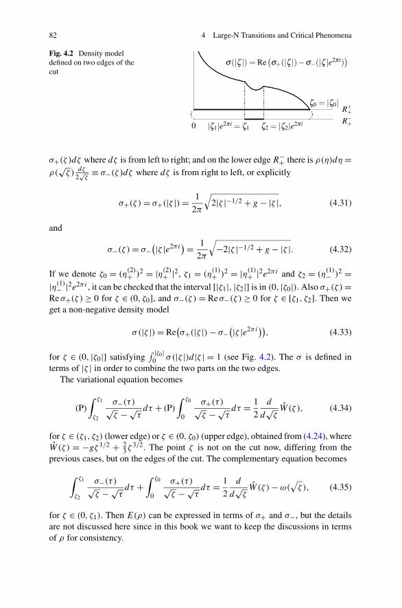
82 4 Large-N Transitions and Critical Phenomena
Fig. 4.2 Density modeldefined on two edges of thecut
σ+(ζ )dζ where dζ is from left to right; and on the lower edge R−+ there is ρ(η)dη=ρ(
√ζ )
dζ
2√ζ
≡ σ−(ζ )dζ where dζ is from right to left, or explicitly
σ+(ζ )= σ+(|ζ |)= 1
2π
√2|ζ |−1/2 + g − |ζ |, (4.31)
and
σ−(ζ )= σ−(|ζ |e2πi)= 1
2π
√−2|ζ |−1/2 + g − |ζ |. (4.32)
If we denote ζ0 = (η(2)+ )2 = |η(2)+ |2, ζ1 = (η
(1)+ )2 = |η(1)+ |2e2πi and ζ2 = (η
(1)− )2 =
|η(1)− |2e2πi , it can be checked that the interval [|ζ1|, |ζ2|] is in (0, |ζ0|). Also σ+(ζ )=Reσ+(ζ ) ≥ 0 for ζ ∈ (0, ζ0], and σ−(ζ ) = Reσ−(ζ ) ≥ 0 for ζ ∈ [ζ1, ζ2]. Then weget a non-negative density model
σ(|ζ |)= Re(σ+(|ζ |)− σ−
(|ζ |e2πi)), (4.33)
for ζ ∈ (0, |ζ0|] satisfying∫ |ζ0|
0 σ(|ζ |)d|ζ | = 1 (see Fig. 4.2). The σ is defined interms of |ζ | in order to combine the two parts on the two edges.
The variational equation becomes
(P)∫ ζ1
ζ2
σ−(τ )√ζ − √
τdτ + (P)
∫ ζ0
0
σ+(τ )√ζ − √
τdτ = 1
2
d
d√ζW (ζ ), (4.34)
for ζ ∈ (ζ1, ζ2) (lower edge) or ζ ∈ (0, ζ0) (upper edge), obtained from (4.24), whereW (ζ ) = −gζ 1/2 + 2
3ζ3/2. The point ζ is not on the cut now, differing from the
previous cases, but on the edges of the cut. The complementary equation becomes
∫ ζ1
ζ2
σ−(τ )√ζ − √
τdτ +
∫ ζ0
0
σ+(τ )√ζ − √
τdτ = 1
2
d
d√ζW (ζ )−ω(
√ζ ), (4.35)
for ζ ∈ (0, ζ1). Then E(ρ) can be expressed in terms of σ+ and σ−, but the detailsare not discussed here since in this book we want to keep the discussions in termsof ρ for consistency.

4.1 Cubic Potential 83
4.1.3 Fifth-Order Phase Transition
For the fifth-order discontinuity discussed in the following, it is convenient to usethe parameter a as the transition variable since g = 2a2 + a−1 is not monotonic ona ∈ (0,1). The potential is now written as W(η)= −(2a2 + a−1)η+ 2
3η3.
Consider the densities in terms of the parameter a,
ρ(η)={
1π
√A+ 2η+ (2a2 + a−1)η2 − η4, 0 < a ≤ 2−2/3,
1π(η+ a)
√a−1 − (η− a)2, 2−2/3 ≤ a ≤ 1,
(4.36)
where the first density is defined for η on Ω to be given next, and A is given by(4.14).
Lemma 4.4 The density defined by (4.36) satisfies
ρ(η)={
1π(η+ η0)
√2a2 + 2aη0 − (η− η0)2, 0 < a ≤ 2−2/3,
1π(η+ a)
√a−1 − (η− a)2, 2−2/3 ≤ a < 1,
(4.37)
for η ∈Ω , where Ω = [η0 −√2a2 + 2aη0, η0 +√2a2 + 2aη0] when 0 < a ≤ 2−2/3
with
η0 = (√a2 + 2a−1 − a
)/2 → 22/3,
(as a → 2−2/3) (4.38)
satisfying 2aη20 + 2a2η0 − 1 = 0, η4
0 − η0 + A = 0 and −η0 ≤ −a ≤ η0 −√2a2 + 2aη0; and Ω = [a − a−1/2, a + a−1/2] when 2−2/3 ≤ a < 1 with the pa-
rameter a satisfying −a ≤ a − a−1/2.
Proof It can be checked that when 0 < a ≤ 2−2/3 there is
η4 − (2a2 + a−1)η2 − 2η−A= (η+ η0)2((η− η0)
2 − 2a2 − 2aη0).
Here, −η0 is on the left side of the interval where the eigenvalue density ρ is definedon. The rest of the lemma can be verified by the elementary calculations. �
Define
ω(η)={(η+ η0)
√(η− η0)2 − 2a2 − 2aη0, 0 < a ≤ 2−2/3,
(η+ a)√(η− a)2 − a−1, 2−2/3 ≤ a ≤ 1,
(4.39)
in the complex plane outside the cut Ω . We see that ω(η) satisfies
ω(η)= 1
2W ′(η)− η−1 +O
(η−2), (4.40)
as η → ∞, and then
(P)∫
Ω
ρ(λ)
η− λdλ= 1
2W ′(η), η ∈Ω, (4.41)

84 4 Large-N Transitions and Critical Phenomena
where W(η)= −(2a2 + a−1)η+ 23η
3 and ′ = ∂/∂η. Now, consider
E(a)=∫
Ω
(2
3η3 − (2a2 + a−1)η
)
ρ(η)dη−∫
Ω
∫
Ω
ln |λ− η|ρ(λ)ρ(η)dλdη.(4.42)
Since ρ is defined on one interval in both a ≤ 2−2/3 and a ≥ 2−2/3 cases, the first-order derivatives in these two cases have the following formulation,
d
daE(a)= −(4a − a−2)
∫
Ω
ηρ(η)dη, (4.43)
that implies
d
daE(a)=
{−a5 + 5
4a2 − 1
4a−1 − (a5 − 1
4a2)(1 + 2a−3)3/2, 0 < a ≤ 2−2/3,
−4a2 + 12a
−1 + 18a
−4, 2−2/3 ≤ a < 1.(4.44)
By direct calculations, one can find that the E function has continuous derivativesup to the fourth order with the values 0, −9×21/3, 36 and −252×22/3 of djE/daj
for j = 1,2,3,4 respectively at a = 2−2/3. But the fifth-order derivative is not con-tinuous. Then we get a fifth-order transition model summarized in the following.
Theorem 4.2 When 0 < a < 1, the E function (4.42) has continuous derivativesdjE/daj for j = 1,2,3,4, but the fifth-order derivative is discontinuous at thecritical point a = 2−2/3.
However, when a > 2−2/3 if we consider the transition in the g direction,
g = 2a2 + a−1, (4.45)
a power-law divergence occurs at the third-order derivative at the critical point gc =3 × 2−1/3 which is corresponding to a = 2−2/3. By (4.44) for a > 2−2/3, it is nothard to get that
dE(g)
dg= −a − 1
8a−2, (4.46)
andd2E(g)
dg2= −1
4a−1. (4.47)
Since (4.45) permits the following expansions
g = gc + ε2, a = 2−2/3 + 6−1/2ε+ · · · , (4.48)
we then have the power-law divergence for the third-order derivative in the g direc-tion
d3E(g)
dg3=O
(1
|g − gc|1/2
)
, (4.49)
as g → gc + 0.

4.1 Cubic Potential 85
The above discussion has changed the fifth-order discontinuity to the third-orderpower-law divergence. Can we further change the third-order divergence to a first-order divergence? If we make the following change of variable
x = 2
3a3 − 3 × 2−1/3a + lna, a > 2−2/3, (4.50)
which is an monotonic increasing function for a > 2−2/3, then since
dx
da= 2(1 + 21/3a−1)(a − 2−2/3)2, (4.51)
the formula (4.44) for a > 2−2/3 can be changed to
dE(x)
dx= (8a3 + 1)(a2 + 2−2/3a + 2−4/3)
4a3(a + 21/3)(a − 2−2/3). (4.52)
It can be checked that as a → 2−2/3 + 0, there is
x − xc = 2(a − 2−2/3)3 +O
((a − 2−2/3)4), (4.53)
where xc = − 43 − 2
3 ln 2. Therefore, we have
dE(x)
dx=O
(1
|x − xc|1/3
)
, (4.54)
as x → xc + 0. So we get a first-order divergence.Also, the critical point can be determined by considering the vanishing case of
dg
da= 4a − a−2, (4.55)
based on the relation g = 2a2 + a−1 given above that also implies
g = 2(a − 2−2/3)2 + (22/3 − a−1/2)2 + 3 × 2−1/3 ≥ 3 × 2−1/3, (4.56)
for a > 0.The above examples give a indication that in some cases the high order transition
models can be reduced to low order transitions by properly changing the transitionvariable. In this situation, the string equations can play an important role to inves-tigate the first-order transition problems. We have seen that the nonlinear relationsobtained from the string equations can give the fractional power-law divergencefor the first-order transition which is generally believed in statistical mechanics tobe harder than the second-order transition problems. The above discussions are allabout the odd order transitions. We will discuss in the next section that the second-order divergence of the free energy (critical phenomenon) can be obtained by usingboth string equation and Toda lattice.

86 4 Large-N Transitions and Critical Phenomena
4.2 Quartic Potential
Now, let us consider the model with the potential V (z)= t2z2 + t4z
4. By the orthog-onality, we have
pn,z = −vnzpn + vn[2t2 + 4t4
(vn + vn+1 + z2)]pn−1, (4.57)
and the vn’s satisfy the string equation,(2t2 + 4t4(vn + vn−1 + vn+1)
)vn = n. (4.58)
Denote Φn = e− 12V (z)(pn,pn−1)
T . Equation (4.57) is then changed to [11]
Φn,z =AnΦn, (4.59)
where
An =( −2t4z3 − t2z− 4t4vnz vn(4t4z2 + 2t2 + 4t4(vn + vn+1))
−4t4z2 − 2t2 − 4t4(vn + vn−1) 2t4z3 + t2z+ 4t4vnz
)
.
(4.60)Consequently, there is
−detAn = 4t24 z6 + 4t4t2z
4 + (t22 − 4t4n)z2 − vn
(
t + 2t4vn + n
2vn
)2
+ 4t24(v′n)
2
vn.
(4.61)If we make the following scalings
t
n1/2= g2 + ξ
n, z= n1/4η, vn = n1/2v, (4.62)
then
−detAn = n3/2(
1
4η6 + g2η
4 + (g22 − 1
)η2 −X+O
(n−1)
)
, (4.63)
where
X = 4v(g2 + 4g4v)2 − 4g2
4
v2ξ
v, (4.64)
where
2g2v + 12g4v2 = 1. (4.65)
One may use the method discussed in Appendix D to find the singular valuesfor X. The corresponding coefficient matrix C would be a 6 × 6 matrix. Here, wejust consider three possible singular cases
X =X(g2)=
⎧⎪⎨
⎪⎩
4g2(9g22 − 1),
4v(g2 + 4g4v)2,
0,
(4.66)

4.2 Quartic Potential 87
in order to give some second-order transition examples. The formula X =4g2(9g2
2 − 1) is obtained such that the right hand side of (4.63) can be so fac-torized as shown next when n goes to infinity. Without loss of generality in thecase g4 > 0, we are going to discuss the transition between X = 4g2(9g2
2 − 1) andX = 4v(g2 + 4g4v)
2 next by taking g4 = 1/4 for convenience in discussion. Thetransition between X = 4v(g2 + 4g4v)
2 with g4 > 0 and X = 0 has been studied inSect. 3.5.
4.2.1 Second-Order Transition
Consider
ρ(η)={
1π
√(4g2 − η2)(( 1
2η2 + 2g2)2 + 5g2
2 − 1), 1/3 < g2 ≤ 1/√
5,1π(g2 + v + 1
2η2)√
4v − η2, g2 ≥ 1/√
5,(4.67)
where the equation ( 12η
2 + 2g2)2 + 5g2
2 − 1 = 0 has four pure imaginary roots±iη1 and ±iη2 because 1 − 5g2
2 < (2g2)2, and they become to ±i2/51/4 as
g2 → 1/√
5 − 0. When g2 ≥ 1/√
5, g2 and v are related by 2g2v + 3v2 = 1 asgiven before.
When g2 ≥ 1/√
5, the derivative of the free energy has the following formula
dE
dg2=∫ 2
√g2
−2√g2
η2ρ(η)dη. (4.68)
When g2 ≤ 1/√
5, the eigenvalues are still distributed on one interval on the realline, but the phase includes two cuts in the complex plane, that is a case l1 = 1 andl2 = 2 discussed in Sect. 2.4. Since the variational equation only involves one inter-val on the real line, the calculation for the first-order derivative of the free energy isstill like the g2 ≥ 1/
√5 case. So the above formula is true for the two cases. By the
asymptotics√
1
4η6 + g2η4 + (g2
2 − 1)η2 −X
= 1
2η3 + g2η− η−1 − 12g2
(6g2
2 − 1)η−3 +O
(η−5), (4.69)
as η → ∞, where X = 4g2(9g22 − 1), we then get
dE
dg2= 6g2
(6g2
2 − 1), 1/3 < g2 ≤ 1/
√5. (4.70)
Note that in the contour integral calculations, the cuts in the complex plane areinvolves, but these parts are canceled when we take the real or imaginary parts due

88 4 Large-N Transitions and Critical Phenomena
to the complex conjugates. Hence, there is
d2E
dg22
= 6(18g2
2 − 1), 1/3 < g2 ≤ 1/
√5. (4.71)
It has been obtained in Sect. 3.5 that
dE
dg2= v(v2 + 1
), g2 ≥ 1/
√5, (4.72)
and
d2E
dg22
= 2v2, g2 ≥ 1/√
5, (4.73)
where 2g2v+ 3v2 = 1. Therefore dE/dg2 is continuous and d2E/dg22 is discontin-
uous at the critical point g2 = 1/√
5 with v = 1/√
5,
E′(1/√
5 − 0)= 6
5√
5=E′(1/
√5 + 0),
E′′(1/√
5 − 0)= 78
5>
2
5=E′′(1/
√5 + 0).
(4.74)
This example shows that the string equations can also create second-order transi-tion models while the discussions before are all about first- or third-order transitionmodels. The difference between this model and others is the four complex rootstalked above. In the first-order discontinuity model in Sect. 4.1, there is no complexroot.
4.2.2 Critical Phenomenon
The planar diagram model [3] is the case X = 4v(g2 + 4g4v)2 with g4 < 0, and
the density has been discussed in Sect. 2.5. We want to study whether the planardiagram model has a transition or divergence at the critical point g2
2 + 12g4 = 0,which was originally given as g2 = 1/2 and g4 = −1/48 in [3]. One can try to usethe hypergeometric-type equation to find a transition for the planar diagram model.As talked above, the coefficient matrix for the hypergeometric-type equation wouldbe a 6 × 6 matrix, and the calculations will be complicated. The discussion in thefollowing based on the double scaling will involve the parameter n in the transition,which is not directly included in the X variable talked before. The method is thendifferent from the hypergeometric-type differential equation. We will first discussthe divergence of the third-order derivative of the free energy at g2 = gc2, that canbe obtained based on the algebraic equation derived from the string equation by us-ing the ε-expansion method. Then in the t2 direction, the second-order derivative is

4.2 Quartic Potential 89
divergent at the critical point t2 = √ngc2, that is a critical phenomenon. This subsec-
tion is planned to discuss the main steps in deriving the divergences for the planardiagram model. The details will be given in next section for the generalized planardiagram model.
Based on (4.65), denote
Rc = 2gc2 + 12gc4v − v−1, (4.75)
where gc2 = v−1c and gc4 = − 1
12v−2c with a constant number vc > 0. Let
v = vc(1 + αε+ · · · ). (4.76)
We have
Rc = −α2v−1c ε2 + · · · . (4.77)
According to the restriction condition 2g2 + 12g4v − v−1 = 0 and (4.77), if g4 isa constant g4 = gc4, then we need to choose g2 = gc2 + ε2 to have the coefficientof ε2 in the restriction condition equal to 0. Then we get α2 = 2vc that impliesdv/dg2 =O(ε−1). Since d2E/dg2
2 = −2v as discussed in last chapter, there is
d3E(g2)
dg32
= −2dv
dg2=O
(|g2 − gc2|−1/2), (4.78)
as g2 → gc2 + 0. If we consider g2 = gc2 and g4 = gc4 + ε2, there is α2 = 12vc. Sinced2E/dg2
4 = −36v4, there is a corresponding power-law divergence d3E(g4)/dg34 =
O(|g4 − gc4|−1/2) as g4 → gc4 + 0. The critical point in the above third-order diver-gence can be directly obtained from the relation 2g2 + 12g4v− v−1 = 0. If we takeg4 as a negative constant and consider the vanishing point of
dg2
dv= −6g4 − 1
2v2, (4.79)
then the critical point is obtained as gc2 = 2√−3g4 when v = 1/
√−12g4. And gc2is the lower bound of g2 since g2 = 1
2 (v−1 + 12(−g4)v) ≥ 2
√−3g4 = gc2, thatindicates we need to use different method to discuss the case g2 < gc2. We caninvestigate the density model when g2 < gc2 based on the general density model
1nπ
√detAn(z)dz, in which case the gj parameters need to be changed to the tj pa-
rameters. It will be discussed in Sect. 4.3.1 that the second-order derivative of thefree energy function is consistent with the formula ∂2 lnZn/∂t
22 = vn(vn+1 + vn−1)
when the density above is on one interval with some cuts in the complex plane.Then the first- and second-order derivatives of the free energy function are contin-uous at the critical point for the planar diagram model, even the models on the twosides of the critical point look quite different. This discussion at least brings theinformation that the planar diagram model is like the Gross-Witten model that theyboth have third-order discontinuity or divergence. The interesting thing is that these

90 4 Large-N Transitions and Critical Phenomena
models and their generalizations, to be discussed in next section, have second-orderdivergences if we slightly change the direction of the transition as explain in thefollowing.
The formula above can be changed to a new expression
∂2
∂t22
lnZn = 2vnvn−1 − dvn
dt2, (4.80)
by using the relation vnvn+1 = vnvn−1 − dvn/dt2 in order to eliminate the indexn+1 in the formula and get a closed system since in the formula of Zn there are justn random variables zj (1 ≤ j ≤ n). This change more clearly shows the dynamics ofthe model in the t2 direction, and we can study what can happen in the t2 directionin large-N asymptotics. It will be discussed in Sect. 4.3.3 by using double scalingthat the string equation (2t2 + 12t4(vn−1 + vn + vn+1))vn = n can be reduced to anonlinear differential equation in the t2 direction with the asymptotics t2 = tc2 (1 +O(n−4/5)) and vn = vcn(1 +O(n−2/5)). So we have dvn/dt2 =O(|t2 − tc2 |−1/2) ast2 → tc2 − 0, that implies the critical phenomenon (second-order divergence)
∂2 lnZn
∂t22
=O
(1
|t2 − tc2 |1/2
)
, (4.81)
as t2 → tc2 − 0, where tc2 = √ngc2 to be discussed later in the double scaling. When
the parameter passes the critical point, the vn and vn+1 will be scaled in the sameway to get back to the planar diagram model in the region g2 > gc2, where the diver-gence occurs at the third-order derivatives of the free energy function as discussedabove.
The third-order and second-order divergences are mutually related each other,that show the singularities in the different directions, g2 or t2. The t2 direction seemslocal since the tc2 involves parameter n, while in the g2 direction, the parameter ncompletely disappears. If we compare the divergences with the discontinuities, itmay be found that the divergence comes from the slight change of the integrablesystem, and the discontinuities are due to relatively heavy changes, although all thereductions are just tiny deformations from the integrable systems. The third-ordertransition models discussed in last chapter are based on the periodic reduction onthe Lax pair by replacing un−lq+s−1 and vn−lq+s by x(s)n and y(s)n respectively. Theabove divergences are obtained by considering the singularities of the X variable inlarge-N asymptotics.
The density models for the second-order transitions in the discussion for the t2direction above and Sect. 4.2.1 have cuts in complex plane that are different fromother density models we have talked before. This would indicate that the second-order transition models do not completely stay in the momentum aspect. In fact, theToda lattice involved in the discussion is a dynamic model that is researched to findthe position properties. And the large-N asymptotics to be discussed in Sect. 4.3.3transforms the string system to a differential equation system which is equivalentto the KdV system [11], indicating a relation to the position aspect at the critical

4.3 General Quartic Potential 91
point. In the second-order transition model considered in Sect. 4.2.1, there are com-plex roots in the first density in (4.67), which become ±i2/51/4 as g2 → 1/
√5. The
large-N reduction of the discrete integrable system to the KdV system discussed in[11] is at a complex point z= iy0, say, for the 2D quantum gravity model. The cor-responding density problems with cuts in the complex plane might be related to thedifferent types of large-N asymptotics with complex coefficients. These propertiesraise new problems such as the correspondences between the complex numbers inthe different methods, and introduce a possibility to understand the singularities inthe second-order transition problems.
Furthermore, it is known that the KdV system can be reduced to a second-ordertransition model by the q-periodicity constraints kj+M = qkj and θ
(0)j+M = θ
(0)j for
the parameters in the τ -function of the KdV equation discussed in [16–18] by Lout-senko and Spiridonov. It is unknown whether there is a relation between the periodicconstraint and the periodic reduction in the string equation discussed above. Also,the string system can give the critical phenomenon as discussed in this section, thatis usually studied in the renormalization group theory. The integrable systems pro-vide a structure to balance the invariance and the renormalization by properly work-ing on the reduction in the discrete or continuum direction(s). Interested readers canfind more discussions in the literatures, for example, [1, 2, 4, 7–10, 12, 13, 15, 22](matrix models and phase transitions), [5, 14] (phase transition in quantum chromo-dynamics), [6, 19, 21] (Wilson loops) and much more. In the next section, we willdiscuss the general quartic potential to extend the planar diagram model and analyzewhat a difference it will make.
4.3 General Quartic Potential
4.3.1 Density Model with Discrete Parameter
Now, we are going to discuss the transition for a generalized planar diagram modelfor the potential
V (z)= t1z+ t2z2 + t3z
3 + t4z4, (4.82)
with the technical details that have been omitted in Sect. 4.2.2. The following resultsare based on the Lax pair discussed in Chap. 2.
Consider the orthogonal polynomials pn(z) = zn + · · · defined by 〈pn,pn′ 〉 ≡∫∞−∞ pn(z)pn′(z)e−V (z)dz= hnδnn′ . The recursion formula
pn+1(z)+ unpn(z)+ vnpn−1(z)= zpn(z), (4.83)
where vn = hn/hn−1 > 0 can be written as
Φn+1 = Ln(z)Φn, (4.84)

92 4 Large-N Transitions and Critical Phenomena
where
Ln(z)=(z− un −vn
1 0
)
. (4.85)
And Φn(z)= e− 12V (z)(pn(z),pn−1(z))
T also satisfies
∂
∂zΦn =An(z)Φn, n≥ 2, (4.86)
where
An(z)=(
γn vnδn−δn−1 −γn
)
,
γn = −vn(3t3 + 4t4(un + un−1 + z)
)− 1
2V ′(z),
δn = 2t2 + 3t3un + 4t4(u2n + vn + vn+1
)+ (3t3 + 4t4un)z+ 4t4z2.
(4.87)
The coefficients un and vn are functions of the potential parameters tj , j =1,2,3,4. Initially, u0 = 〈z,1〉/h0 and v0 = 0 corresponding to p1 + u0p0 = zp0,where p0 = 1. Also, u1 = 〈zp1,p1〉/h1 and v1 = 〈zp1,1〉/h0. When n≥ 2, un andvn can be obtained from the recursion relations
[2t2 + 3t3(un + un−1)+ 4t4
(u2n + u2
n−1 + unun−1 + vn+1 + vn + vn−1)]vn = n,
(4.88)
t1 + 2t2un + 3t3(u2n + vn+1 + vn
)+ 4t4(u3n + (un+1 + 2un)vn+1
+ (2un + un−1)vn)= 0, (4.89)
which are derived from the following relations based on the orthogonality of thepolynomials
⟨pn(z),V
′(z)pn−1(z)⟩= nhn−1,
⟨pn(z),V
′(z)pn(z)⟩= 0,
where n ≥ 1. The set of the two discrete equations (4.88) and (4.89) for un and vnis called string equation. The consistency condition for (4.86) and (4.84) is of theform ∂Ln/∂z = An+1Ln − LnAn. It can be verified by direct calculations that thisconsistency condition is equivalent to (4.88) and (4.89). So (4.86) and (4.84) arecalled the Lax pair for the string equation, and then we get a discrete integrable sys-tem. In Sect. 4.3.3, we will discuss in what situation the discrete integrable systemcan be reduced to a continuum integrable system by double scaling in order to findwhat causes the discontinuity of the free energy. But first, let us work on the basicproperties to get ready for discussing the transition problem.
Since the roots of detAn = 0 may be distributed on the real line or in the complexplane as the parameter n changes, it is uncertain to conclude what a density model

4.3 General Quartic Potential 93
√detAn can create. If detAn = 0 has four or six real roots, that are the cases like
the model discussed in Sect. 4.1.2. In the following, let us consider a case of tworeal roots z1 and z2 with four complex roots z3, z4 and their complex conjugates z3and z4, where z3 and z4 are in the upper half plane, say. Then the density is like acase discussed in Sect. 2.4 with l = l1 + l2 where l1 = 1 and l2 = 2 with the formula
ρ(z,n)= 1
nπRe√
detAn(z), −∞< z <∞, (4.90)
or ρ(z,n)= 1nπ
√detAn(z) for z1 ≤ z≤ z2, satisfying
∫ z2
z1
ρ(z,n)dz= 1, (4.91)
and
(P)∫ z2
z1
ρ(ζ,n)
z− ζdζ = 1
2nV ′(z), (4.92)
according to the discussions in Sects. 2.3 and 2.4, where ′ = ∂/∂z and z is an innerpoint in [z1, z2], that implies∫ z2
z1
ln |z− ζ |ρ(ζ,n)dζ − 1
2nV ′(z)=
∫ z2
z1
ln |z1 − ζ |ρ(ζ,n)dζ − 1
2nV ′(z1).
If the free energy function is defined as
E = 1
n
∫ z2
z1
V (z)ρ(z,n)dz−∫ z2
z1
∫ z2
z1
ln |z− ζ |ρ(z,n)ρ(ζ, n)dzdζ,
then the first-order derivative in the t2 direction is
∂E
∂t2= 1
n2πRe∫ z2
z1
z2√
detAndz, (4.93)
by the similar discussion as in Sect. 3.4. To further compute the derivative of thisintegral, we need the consistency condition
An,t2 =Mn,z +MnAn −AnMn, (4.94)
where ∂Φn/∂t2 =MnΦn, which together with (4.84) form the Lax pair for the Todalattice in the t2 direction, to reduce the complexity by the coefficient matrix Mn forthe linear equation in the t2 direction, where
Mn =(− 1
2z2 − vn vn(z+ un)
−z− un−112z
2 − u2n−1 − vn−1
)
. (4.95)
Since A2n − (trAn)An + (detAn)I = 0 where trAn = 0, we have detAn = − 1
2 trA2n,
that implies

94 4 Large-N Transitions and Critical Phenomena
(detAn)t2 = − tr(AnAn,t2)
= − tr(An(Mn,z +MnAn −AnMn)
)
= − tr(AnMn,z)
= n+ vn(2t2 + 4t4
(vn − unun−1 − (un + un−1)z
))− zV ′(z),
by using the string equation. Since
∂2E
∂t22
= 1
4n2πRe
1
i
∫
Ω∗z2 (detAn)t2√−detAn(z)
dz, (4.96)
where Ω∗ is the contour around [z1, z2], and√−detAn = 1
2V′(z)−nz−1 +O(z−2)
as z→ ∞, there is
∂2E
∂t22
= − 1
n2vn(vn+1 + vn−1 + (un + un−1)
2), (4.97)
by noting that the contour integrals around the cuts between z3 and z4 and betweenz3 and z4 are canceled by taking the real part because all the parameters are real.We see that the result above is consistent with the formula ∂2 lnZn/∂t
22 = vn(vn+1 +
vn−1 + (un + un−1)2) obtained in Sect. 3.2.
4.3.2 Expansion for the Generalized Model
We are going to discuss the transition between the ρ(z,n) given above and thegeneralized planar diagram density
ρ(η)= 1
2π
(2g2 +3g3(η+a)+4g4
(η2 +aη+a2 +2b2))
√4b2 − (η− a)2, (4.98)
given in Sect. 2.5, with the parameters satisfying the following conditions
2g2 + 3g3(η+ a)+ 4g4(η2 + aη+ a2 + 2b2)≥ 0, η ∈ [η−, η+], (4.99)
2g2b2 + 6g3ab
2 + 12g4(a2 + b2)b2 = 1, (4.100)
g1 + 2g2a + 3g3(a2 + 2b2)+ 4g4a
(a2 + 6b2)= 0, (4.101)
where η± = a± 2b. It has been discussed that this one-interval density model satis-fies the following properties
∫ η+
η−ρ(η)dη = 1, (4.102)

4.3 General Quartic Potential 95
and
(P)∫ η+
η−
ρ(λ)
η− λdλ= 1
2W ′(η), (4.103)
where W(η) =∑4j=0 gjη
j and ′ = ∂/∂η. These equations do not have parametern, while the equations (4.91) and (4.92) for ρ(z,n) involve the parameter n. Theparameter n can provide the large-N asymptotics to meet with the singularity fromthe ρ(η) model as explained in the following.
Differing from the bifurcation transition discussed in Chap. 3, the transition dis-cussed in this section is a case that at the critical point the parameters satisfy thecondition
2g2 + 3g3(η+ a)+ 4g4(η2 + aη+ a2 + 2b2)= 4g4
((η− a)2 − 4b2). (4.104)
That means the factor outside the square root in the formula of the ρ(η) approachesto the phase in the square root at the critical point. By comparing the coefficients onboth sides of the equation above, it is not hard to see that the parameter values at thecritical point satisfy
gc1 = − 5
3bc, 2gc2 = 1
b2c
, 3gc3 = 1
b3c
, 4gc4 = − 1
3b4c
, ac = bc.
(4.105)And the density ρ(η) becomes 1
6πb4c(4b2
c − (η − bc)2)3/2. Consider (4.100) and
(4.101). If we take a and b as functions of g2 and all other parameters are constantswith the critical values, then it can be checked that the condition in the implicitfunction theorem is not satisfied at the critical point. That leads us to investigate thedivergence or critical phenomenon around the critical point.
Let us start from the free energy for the density ρ(η). It has been obtained inSect. 3.1 that the free energy function for the density ρ(η) has the following explicitformula
E =W(a)+ 3
4− lnb− 4g4b
4 − 6(g3 + 4g4a)2b6 − 6g2
4b8. (4.106)
We are going to use the ε-expansion method to investigate whether a derivative ofthe free energy has a discontinuity or divergence.
For convenience in discussion, denote
Rc1 ≡ 2gc2 + 6gc3a + 12gc4
(a2 + v
)− v−1, (4.107)
Rc2 ≡ gc1 + 2gc2a + 3gc3
(a2 + 2v
)+ 4gc4a(a2 + 6v
), (4.108)
where v = b2. Now, let us expand a and v in terms of a small parameter ε,
a = bc(1 + α1ε+ α2ε
2 + · · · ), (4.109)
v = b2c
(1 + β1ε+ β2ε
2 + · · · ). (4.110)

96 4 Large-N Transitions and Critical Phenomena
Substituting the expansions (4.109) and (4.110) into (4.107) and (4.108) and com-paring the coefficients of the ε terms, we first have the vanishing O(1) terms,
2gc2 + 6gc3bc + 24gc4b2c − v−1
c = 0,
gc1 + 2gc2bc + 3gc3b2c + 4gc4b
3c + 2
(3gc3 + 12gc4bc
)b2c = 0,
according to the critical values given above. For the O(ε) terms, the coefficients ofε for both R1 and R2 also vanish,
(6gc3bc + 24gc4b
2c
)α1 + (12gc4b
2c + b−2
c
)β1 = 0,
(2gc2bc + 6gc3b
2c + 36gc4b
3c
)α1 + (6gc3b2
c + 24gc4b3c
)β1 = 0,
without any condition for α1 or β1. This has indicated a different style if we com-pare with the expansions in Sect. 3.4. For the O(ε2) terms, the coefficients can becombined and simplified as the following,
(6gc3bc + 24gc4b
2c
)α2 + (12gc4b
2c + b−2
c
)β2 + 12gc4b
2cα
21 − b−2
c β21 = − 1
b2c
(α2
1 + β21
),
(2gc2bc + 6gc3b
2c + 36gc4b
3c
)bcα2 + (3gc3b2
c + 12gc4b3c
)α2
1 + (6gc3b2c + 24gc4b
3c
)β2
+ 24gc4b3cα1β1 = − 2
bcα1β1.
We will use these terms to find the expansion of g2.Since a and v are restricted by the conditions
R1 ≡ 2g2 + 6g3a + 12g4(a2 + v
)− v−1 = 0, (4.111)
R2 ≡ g1 + 2g2a + 3g3(a2 + 2v
)+ 4g4a(a2 + 6v
)= 0, (4.112)
we can use gj = gcj + εμ to create new terms to match with the O(ε2) terms dis-
cussed above so that the O(ε2) terms all disappear. If we consider g1 = gc1 + εμ, itcan be found that it does not add any thing to the R1 equation to vanish the O(ε2)
term. So the simplest case is the g2 direction. This is one of the reasons that in ourdiscussions we always consider the g2 direction. Let
g2 = gc2 + ε2, gj = gcj , j = 2. (4.113)
The above discussions yield
R1 =Rc1 + 2ε2 =
[
2 − 1
b2c
(α2
1 + β21
)]
ε2 +O(ε3), (4.114)
R2 =Rc2 + 2aε2 =
[
2bc − 2
bcα1β1
]
ε2 +O(ε3). (4.115)

4.3 General Quartic Potential 97
Since R1 =R2 = 0, we have
α21 + β2
1 = 2b2c , (4.116)
α1β1 = b2c . (4.117)
The solution is α1 = bc and β1 = bc. Then we get the ε-expansions for a and v,
a = bc(1 + bcε+ · · · ), (4.118)
v = b2c (1 + bcε+ · · · ). (4.119)
Now, come back to the free energy (4.106). By the above expansions, we have
E = 1
8− lnbc +O
(ε2), (4.120)
that means the first-order derivative with respect to g2 does not have singularity atthe critical point. Interested readers can experience the higher order terms in theexpansions. The result should be E = 1
8 − lnbc +O(ε2)+O(ε4)+O(ε5), that isdifferent from the expansion discussed in Sect. 3.4 for g4 > 0. The expansion resultsabove are enough to discuss the transition problem as explained in the following.The continuity of the first-order derivative can be seen from the integral formulas.The second-order derivative has the following formula
∂2E
∂g22
= −2v(2a2 + v
), (4.121)
as discussed before, where the singularity is canceled if we use the free energyformula and the parameter conditions. We then have
∂2E
∂g22
= −4b4c − 10b5
cε+O(ε2), (4.122)
where g2 − gc2 = ε2, which implies
∂3E
∂g32
= ± 5b5c
|g2 − gc2|1/2
(1 + o(1)
), (4.123)
where the sign depends we choose ε = −|g2 − gc2|1/2 or ε = |g2 − gc2|1/2, or simply∂3E/∂g3
2 =O(|g2 − gc2|−1/2) as g → gc2 + 0.The continuity of the second-order derivative of the free energy in the g2 direc-
tion can be seen as we connect (4.121) with (4.97). The details should be discussedby using the double scaling as explained next to see how the two sets of parametersare transferred at the critical point. Locally, the divergence singularity is already hid-den in the t2 direction with the parameter n, that can be seen from the second-order

98 4 Large-N Transitions and Critical Phenomena
derivative formula
∂2
∂t22
lnZn = vn(vn+1 + vn−1 + (un + un−1)
2), (4.124)
when the vn+1 is changed to dvn/dt2 as discussed in Sect. 4.2.2. The discontinu-ity does not appear in the g2 direction for the second-order derivative because thelarge-N factor removed such singularity in a global scale. Generally, there would be
various critical phenomena ∂2 lnZn∂t2j
= O(|tj − tcj |−γj ) in the different tj directions.
That could be discussed by using the string equations and Toda lattice, and left forfurther investigations.
4.3.3 Double Scaling at the Critical Point
The nonlinear differential equation
yxx = 6y2 + x, (4.125)
has a Lax pair of the form [11]
ψxx = 2(y + λ)ψ, (4.126)
ψλ = 2yxψ + 4(2λ− y)ψx, (4.127)
that is obtained from the Lax pair of the KdV equation as discussed in [11] where(4.126) is the Schrödinger equation [11]. As a remark, the nonlinear differentialequation (4.125) is called Painlevé I equation in [11]. It is discussed in [11] thatwhen V (z)= t2z
2 + t4z4, the equation (4.88) for vn with the vanishing un’s can be
reduced to (4.125) by using a double scaling. Since their double scaling involvesthe complex coefficients that could be related to the nonlinear Schrödinger equationaccording to some literatures for a purpose different from here and we expect a dou-ble scaling with real coefficients for discussing the density and free energy function,we need to search a different double scaling with real coefficients. In the follow-ing discussions, vn is coupled with un−1, instead of un, because the Jn matrix inSect. 2.2 is defined by un−1 and vn. When the coefficients in the un−1’s expansionare equal to 0 in the following discussions, the double scaling is for the potentialV (z)= t2z
2 + t4z4.
We want to find real parameters ck and the exponents rk in the following doublescaling in large-N asymptotics,
t2 = n12
(
gc2 + c1
nr1x
)
, tj = n1− j4 gcj , j = 1,3,4, (4.128)
un−1 = n14
(
uc + c2
nr2y(x)
)
, vn = n12
(
vc + c3
nr2y(x)
)
, (4.129)

4.3 General Quartic Potential 99
z= n14(zc + c0λh
2), (4.130)
ψn(z)=ψ(x,λ)(1 + o(1)
), (4.131)
with
un = u(n−1)+1 = n14
(
uc + c2
nr2
(
y + yxh+ 1
2yxxh
2 + · · ·))
, (4.132)
vn±1 = n12
(
vc + c3
nr2
(
y ± yxh+ 1
2yxxh
2 + · · ·))
, (4.133)
ψn±1 =ψ ±ψxh+ 1
2ψxxh
2 +O(h3), (4.134)
to reduce the discrete system to the continuum system given above, where ψn =e− 1
2V (z)pn(z)/h1/2n , and h and other parameter values will be given below.
To get (4.126), rewrite (4.83) as
ψn+1 +ψn−1 − 2ψn +(
un
v1/2n+1
+ 2
)
ψn +(v
1/2n
v1/2n+1
− 1
)
ψn−1 = z
v1/2n+1
ψn,
and substitute the double scaling formulas above into it. After some asymptoticcalculations for the leading terms, there is
ψxxh2 +
[1√vc
(
uc + c2y
nr2− c3ucy
2vcnr2
)
+ 2
]
ψ = 1√vc
[
zc + c0λh2 − c3zcy
2vcnr2
]
ψ.
If we choose
zc = uc + 2√vc, (4.135)
c0 = 2√vc, (4.136)
c2√vc + c3 = −2γ 2vc, γ = hnr2/2, (4.137)
then the above equation becomes (4.126), where γ is a constant, that means h =O(n−r2/2).
To get (4.127), write the first equation in (4.86) as
∂
∂zψn = −
[1
2V ′(z)+ vn
(3t3 + 4t4(un + un−1 + z)
)]
ψn
+ [2t2 + 3t3un + 4t4(u2n + vn + vn+1
)+ (3t3 + 4t4un)z
+ 4t4z2]v1/2
n ψn−1.
By the asymptotic calculations, it can be verified that if the parameters additionallysatisfy
r2 = 2
5, γ 5 = 3
2, (4.138)

100 4 Large-N Transitions and Critical Phenomena
gc3 + 4gc4uc = 0, 12gc4v2c = −1, (4.139)
and
2gc2 + 3gc3uc + 4gc4(u2c + 2vc
)+ (3gc3 + 4gc4uc)zc + 4gc4z
2c = 0, (4.140)
gc1 + 2gc2zc + 3gc3z2c + 4gc4z
3c + 2vc
(3gc3 + 4gc4(2uc + zc)
)= 0, (4.141)
then the above equation is reduced to (4.127).If we substitute the double scaling formulas above with
r1 = 2r2, (4.142)
into (4.88) and (4.89), then we get
γ 2yxx = c23 + vcc
22
4gc4c3v3c
y2 − c1
2gc4c3x, (4.143)
c2γ2yxx = −6c2c3
vcy2 − c1uc
2gc4vcx. (4.144)
In the case uc = 0 and c2 = 0, if the parameters satisfy
c1 = − γ 4
6vc, c2 = −ucγ 2, c3 = −vcγ 2, uc = √
vc, (4.145)
then the above two equations (4.143) and (4.144) both become to (4.125). If uc =c2 = 0 and
c1 = − γ 4
3vc, c3 = −2vcγ
2, vc > 0, (4.146)
then (4.144) becomes 0 = 0, and (4.143) becomes (4.125). In the first case, we havethe critical point
gc1 = − 5
3√vc, 2gc2 = 1
vc, 3gc3 = 1
vc√vc, 4gc4 = − 1
3v2c
, (4.147)
which is consistent to (4.105). In the second case, the critical point is
2gc2 = 2
vc, 4gc4 = − 1
3v2c
, (4.148)
with gc1 = gc3 = 0, which is the critical point for the planar diagram model.If we work on the higher degree potential, then the recursion formula still be-
comes the Schrödinger equation, and the z equation Ψn,z =AnΨn becomes a linearequation coupled with the Schrödinger equation to form a Lax pair for the higherorder equation in the continuum hierarchy which is corresponding to the KdV hier-archy. However, the tj equations Ψn,tj =M
(j)n Ψn can not join with the double scal-
ing because the hierarchy does not have the corresponding equations. This property

4.4 Searching for Fourth-Order Discontinuity 101
affects the whole system, and the critical phenomena are researched based on thissingular property. The critical exponent in the critical phenomenon can be studiedbased on the expansions including the important relation r1 = 2r2 discussed above.
The double scaling reveals that a small system at the point z= zc is separated atthe critical point to reduce the discrete integrable system to a physical model suchas the planar diagram model. The release of the small system from the integrablesystem would help us to think about the cause of the transition. The double scalingmethod can also reduce the Hermitian matrix model to another continuum integrablesystem as researched in [2] for the corresponding critical points. In the two-matrixmodels [8–10], the large-N scaling method is applied to study the correlation func-tion by using the loop equation or Schwinger-Dyson equation, which plays a role asthe string equation, in order to get the Yang-Baxter equation. The scalings for thewhole system as discussed in [2, 8–11, 20] and this section, for instance, providea new interpretation for the discontinuity of the transition phenomena, so that wehave more tools to study these challenging problems.
4.4 Searching for Fourth-Order Discontinuity
We have discussed the discontinuities of the first-, second-, third- and fifth-orderderivatives of the free energy before. In this section, we are going to search a fourth-order discontinuity by considering the potential
W(η)= g1η+ g2η2 + g3η
3. (4.149)
We will choose g3 > 0 in the following discussion. The discussion for g3 < 0 issimilar to the g3 > 0 case. By choosing g4 = 0 in (4.98) and the correspondingconditions, we have
ρ2(η)= 1
2π
(2g2 + 3g3(η+ u)
)√4v − (η− u)2, (4.150)
and
R1 ≡ 2g2 + 6g3u− v−1 = 0, (4.151)
R2 ≡ g1 + 2g2u+ 3g3(u2 + 2v
)= 0. (4.152)
The critical point of the fourth-order transition is when the parameters satisfy thecondition
2g2 + 3g3(η+ u)= 3g3(η− u+ 2√v). (4.153)
Combining this condition with (4.151) and (4.152), we get the values or the relationsof the parameters for the critical point,
g1 = −3/(2uc), gc2 = 0, 6gc3ucvc = 1, uc = bc = √vc. (4.154)

102 4 Large-N Transitions and Critical Phenomena
If one wants to discuss the case uc = −√vc, the straight line should be put to the
right side of the semicircle for the density. It can be seen that for the model (4.150),the parameter g2 is positive (g2 ≥ gc2).
Denote
Rc1 ≡ 2gc2 + 6gc3u− v−1, (4.155)
Rc2 ≡ gc1 + 2gc2u+ 3gc3
(u2 + 2v
), (4.156)
with the expansions
u= bc(1 + α1ε+ α2ε
2 + α3ε3 + · · · ), (4.157)
v = vc(1 + β1ε+ β2ε
2 + β3ε3 + · · · ), (4.158)
where ε = g2 − gc2. We have for the O(1) terms,
O(1): 2gc2 + 6gc3bc − v−1c = 0,
gc1 + 2gc2bc + 3gc3(b2c + 2vc
)= 0,
by the relations (4.154). For the O(ε) terms, there are
O(ε): 6gc3bcα1 + v−1c β1,
(2gc2bc + 6gc3b
2c
)α1 + 6gc3vcβ1.
One can experience that if we do not choose β1 = 0, then there will be a contra-diction in the O(ε2) terms. Therefore, we get α = β1 = 0, consequently implyingeasier calculation in the rest analysis. For the O(ε2) terms, we have
O(ε2): 2 + 6gc2bcα2 + v−1
c β2,
2bc + 2gc2bcα2 + 3g3(2b2
cα2 + 2vcβ2).
By choosing g2 = gc2 + ε in order to finally have R1 = Rc1 + 2ε =O(ε3) and R2 =
Rc2 + 2bcα1ε
2 =O(ε3), we get the following equations for the coefficients,
α1 + β1 = −2b2c ,
α2 + β2 = β21 ,
α2 + β2 = −1
2α2
1 − 2b2cα1.
It can be solved that
α1 =(
−2 ± 2√3
)
b2c , β1 = ∓ 2√
3b2c , α2 + β2 = 3
4b4c . (4.159)

4.4 Searching for Fourth-Order Discontinuity 103
Since ∂2E/∂g22 = −2v(v + 2u2), it can be derived by the expansions above that
∂2
∂g22
E = −2b2c
(3b2
c − 8b4cε+ 12b6
cε2 + · · · ), (4.160)
which implies that
∂3
∂g32
E(0+)= 16b6c ,
∂4
∂g42
E(0+)= −48b8c . (4.161)
Now, consider
An(z)=(
αn vnβn−βn−1 −αn
)
, (4.162)
with
αn = −3t3vn − 1
2
(t1 + 2t2z+ 3t3z
2),
βn = 2t2 + 3t3(un + z),
followed by√
detAn(z)=√vnβnβn−1 − α2
n, (4.163)
and1
nπRe√
detAn(z)dz= ρ(η)dη, (4.164)
with the scaling t1n−2/3, t2n−1/3, t3, unn−1/3, un−1n
−1/3, vnn−2/3 and zn−1/3 re-placed by g1, g2, g3, u, u, v and η respectively. Since
1
n5/3π
∫z2 Re
√detAn(z)dz=
∫η2ρ(η)dη, (4.165)
if detAn = 0 has two real roots and two complex roots as n → ∞, then the first-order derivative ∂E/∂g2 is continuous according to the discussion for the one-interval density models. If it is not the case, then it is a first-order discontinuity.
We have obtained in Sect. 3.2 that the second-order derivative of lnZn has thefollowing formula
∂2
∂t22
lnZn = vn(vn+1 + vn−1 + (un + un−1)
2), (4.166)
where Zn is the partition function. To investigate the continuity of the higher orderderivatives, the derivatives of the un and vn are needed since the expansion methoddoes not work when the model keeps the n parameter. It is not hard to get
2t2 + 3t3(un + un−1)= n
vn, (4.167)

104 4 Large-N Transitions and Critical Phenomena
t1 + 2t2un + 3t3(u2n + vn + vn+1
)= 0, (4.168)
and
∂un
∂t2= −(un+1 + un)vn+1 + (un + un−1)vn, (4.169)
∂vn
∂t2= −vn
(vn+1 − vn−1 + u2
n − u2n−1
). (4.170)
The parameters at the critical point satisfy
t2 = 0, 3t3(un + un−1)vn = n. (4.171)
By these relations, it can be derived that
∂un
∂t2= − 1
3t3+ 2t2
3t3(vn+1 − vn), (4.172)
∂vn
∂t2= 2t2
3t3vn(un − un−1), (4.173)
which imply at the critical point,
∂un
∂t2= − 1
3t3,
∂vn
∂t2= 0. (4.174)
Denote
Sn = vn(vn+1 + vn−1), Tn = vn(un + un−1)2,
for the right hand side of (4.166), and change them to the following by using (4.167)and (4.168),
Sn = −2t23t3
vn − 2t2(3t3)2
(n− 2t2vn)− (u2n + u2
n−1
)vn − 2v2
n,
Tn = vn
(3t3)2
(n
vn− 2t2
)2
.
The derivatives of Sn and Tn with respect to t2 have complicated formulas. But atthe critical point t2 = 0 with un ∼ un−1, vn+1 ∼ vn and un ∼ √
vn, there are thefollowing based on the results obtained above,
∂
∂t2Sn = 0,
∂2
∂t22
Sn = 0, (4.175)
and
∂
∂t2Tn = − 4n
(3t3)2,
∂2
∂t22
Tn = 8vn(3t3)2
. (4.176)

References 105
Then, at the critical point there are
∂3
∂t32
lnZn = − 4n
(3t3)2,
∂4
∂t42
lnZn = 8vn(3t3)2
, (4.177)
which imply that E = limn→∞ −1n2 lnZn satisfies
∂3
∂g32
E(0−)= 16b6c ,
∂4
∂g42
E(0−)= −32b8c . (4.178)
Summarizing the discussions above, we have that if bc = 0 then in the g = g2direction there are
∂j
∂gj
2
E(0−)= ∂j
∂gj
2
E(0+), j = 2,3, (4.179)
∂4
∂g42
E(0−)= −32b8c >−48b8
c = ∂4
∂g42
E(0+). (4.180)
If the first-order derivative is continuous as explained above, then this is a fourth-order discontinuity model with a O(1) discontinuity at the critical point g2 = 0.
References
1. Bertola, M., Marchal, O.: The partition of the two-matrix models as an isomonodromic τ
function. J. Math. Phys. 50, 013529 (2009)2. Bleher, P., Eynard, B.: Double scaling limit in random matrix models and a nonlinear hierarchy
of differential equations. J. Phys. A 36, 3085–3106 (2003)3. Brézin, E., Itzykson, C., Parisi, G., Zuber, J.B.: Planar diagrams. Commun. Math. Phys. 59,
35–51 (1978)4. Chekhov, L., Mironov, A.: Matrix models vs. Seiberg–Witten/Whitham theories. Phys. Lett.
B 552, 293–302 (2003)5. Douglas, M.R., Kazakov, V.A.: Large N phase transition in continuum QCD in two-
dimensions. Phys. Lett. B 319, 219–230 (1993)6. Douglas, M.R., Shenker, S.H.: Strings in less than one dimension. Rutgers preprint RU-89-34
(1989)7. Eynard, B.: Topological expansion for the 1-Hermitian matrix model correlation functions.
J. High Energy Phys. 0411, 031 (2004)8. Eynard, B., Orantin, N.: Topological expansion of the 2-matrix model correlation functions:
diagrammatic rules for a residue formula. J. High Energy Phys. 12, 034 (2005)9. Eynard, B., Orantin, N.: Mixed correlation functions in the 2-matrix model, and the Bethe
ansatz. J. High Energy Phys. 08, 028 (2005)10. Eynard, B., Orantin, N.: Invariants of algebraic curves and topological expansion. Commun.
Number Theory Phys. 1, 347–452 (2007)11. Fokas, A.S., Its, A.R., Kitaev, A.V.: Discrete Painlevé equations and their appearance in quan-
tum gravity. Commun. Math. Phys. 142, 313–344 (1991)12. Gerasimov, A., Marshakov, A., Mironov, A., Morozov, A., Orlov, A.: Matrix models of 2D
gravity and Toda theory. Nucl. Phys. B 357, 565–618 (1991)

106 4 Large-N Transitions and Critical Phenomena
13. Gorsky, A., Krichever, I., Marshakov, A., Mironov, A., Morozov, A.: Integrability andSeiberg-Witten exact solution. Phys. Lett. B 355, 466–477 (1995)
14. Gross, D.J., Matytsin, A.: Instanton induced large-N phase transitions in two-dimensional andfour-dimensional QCD. Nucl. Phys. B 429, 50–74 (1994)
15. Jurkiewicz, J.: Regularization of one-matrix models. Phys. Lett. B 235, 178–184 (1990)16. Loutsenko, I.M., Spiridonov, V.P.: Self-similar potentials and Ising models. JETP Lett. 66,
747–753 (1997)17. Loutsenko, I.M., Spiridonov, V.P.: Spectral self-similarity, one-dimensional Ising chains and
random matrixes. Nucl. Phys. B 538, 731–758 (1999)18. Loutsenko, I.M., Spiridonov, V.P.: A critical phenomenon in solitonic Ising chains. SIGMA 3,
059 (2007)19. Passerini, F., Zarembo, K.: Wilson loops in N = 2 super-Yang-Mills from matrix model.
J. High Energy Phys. 1109, 102 (2011)20. Pastur, L., Figotin, A.: Spectra of Random and Almost Periodic Operators. Springer, Berlin
(1992)21. Rey, S.-J., Suyama, T.: Exact results and holography of Wilson loops in N = 2 superconformal
(quiver) gauge theories. J. High Energy Phys. 1101, 136 (2011)22. Shimamune, Y.: On the phase structure of large N matrix models and gauge models. Phys.
Lett. B 108, 407–410 (1982)

Chapter 5Densities in Unitary Matrix Models
The unitary matrix model is another important topic in quantum chromodynamics(QCD) and lattice gauge theory. The Gross-Witten weak and strong coupling densi-ties are the most popular density models in QCD for studying the third-order phasetransition problems, which are related to asymptotic freedom and confinement. Forthe Gross-Witten weak and strong coupling densities and the generalizations to bediscussed in this chapter, it should be noted that the densities are defined on the com-plement of the cuts in the unit circle, and there are two essential singularities, whichare different from the Hermitian models. The orthogonal polynomials on the unitcircle are applied to study these problems by using the string equation. The recur-sion formula now becomes the discrete AKNS-ZS system, and the reduction of theeigenvalue density is now based on new linear systems of equations satisfied by theorthogonal polynomials on the unit circle. The integrable systems and string equa-tion discussed in this chapter provide a structure for finding the generalized densitymodels and parameter relations that will be used as the mathematical foundation toinvestigate the transition problems discussed in next chapter.
5.1 Variational Equation
According to the discussion in [4], an eigenvalue density ρ(θ) on an interval ormultiple disjoint intervals Ωθ in [−π,π] for the potential 2
∑mj=1 gj cos(jθ) should
be defined to satisfy ρ(θ)≥ 0,∫Ωθ
ρ(θ)dθ = 1 and the variational equation
(P)∫
Ωθ
cotθ − θ ′
2ρ(θ ′)dθ ′ = 2
m∑
j=1
jgj sin(jθ). (5.1)
Convert the interval [−π,π] to the unit circle by z = eiθ , then Ωθ becomes Ω tobe as an arc or multiple disjoint arcs on the unit circle, and ρ(θ) is changed to σ(z)by ρ(θ)dθ = σ(z)dz. For the potential U(z) =∑m
j=1 gj (zj + z−j ), σ(z) needs to
C.B. Wang, Application of Integrable Systems to Phase Transitions,DOI 10.1007/978-3-642-38565-0_5, © Springer-Verlag Berlin Heidelberg 2013
107

108 5 Densities in Unitary Matrix Models
satisfies∫Ωσ(z)dz= 1 and the variational equation
(P)∫
Ω
ζσ(ζ )
ζ − zdζ = 1
2zU ′(z)+ 1
2, (5.2)
where z is an inner point of Ω , ′ = d/dz, zU ′(z) = z(U ′0(z) + U ′
0(z−1)) =
∑mj=1 jgj (z
j − z−j ) and U0(z) =∑mj=1 gj z
j . Note that σ(z) is not positive, orit is even not a real function. This transformation will make the discussions mucheasier to apply the properties of the analytic functions. If U(z) = T −1(z + z−1),then the variational equation becomes
(P)∫
Ωθ
cotθ − θ ′
2ρ(θ ′)dθ ′ = 2
Tsin θ, (5.3)
or
(P)∫
Ω
ζσ(ζ )
ζ − zdζ = 1
2T
(z− z−1)+ 1
2, (5.4)
where z = eiθ ∈ Ω , θ ∈ Ωθ , Ωθ is corresponding to Ω , and σ(ζ )dζ = ρ(θ ′)dθ ′with ζ = eiθ
′. Equation (5.3) is the original variational equation for the unitary ma-
trix model [4], and (5.4) or the general form (5.2) is derived from it in order to usethe asymptotics in the complex plane to study the density problems.
We have seen in the Hermitian matrix models that the eigenvalue density can beobtained from the coefficient matrix in the Lax pair by discussing the associatedorthogonal polynomials. For the unitary matrix models, it is the same idea, but theprocess is much complicated because now there are two essential singular pointsz= 0 and z= ∞. The details will be discussed in the following sections. Let us stilluse the Gross-Witten density models to explain how to change an eigenvalue densityproblem to an asymptotics problem for an analytic function ω(z). The zω(z) needsto have an asymptotics 1
2z(U′0(z) − U ′
0(z−1)) + 1
2 as z → 0 or z → ∞. Note that12z(U
′0(z)−U ′
0(z−1))+ 1
2 is not 12zU
′(z)+ 12 , that is an important difference from
the Hermitian matrix models. Consider
σ(z)dz={(1 + 1
T(z+ z−1)) dz
2πiz , T ≥ 21T(z1/2 + z−1/2)
√(z1/2 + z−1/2)2 + 2(T − 2) dz
2πiz , T ≤ 2,(5.5)
where σ(z) is defined on Ω = {z||z| = 1} when T ≥ 2, and defined on Ω = {z||z| =1}�Ω when T ≤ 2, where
Ω = {z= eiθ∣∣∣∣cos(θ/2)
∣∣≤√1 − (T /2), |θ | ≤ π
}. (5.6)
Note that Ω is a cut around z = −1, and Ω is the complement of Ω in the unitcircle. Define ω(z) by
zω(z)={
12 (1 + 1
T(z+ z−1)), z ∈C, T ≥ 2
12T (z
1/2 + z−1/2)√(z1/2 + z−1/2)2 + 2(T − 2), z ∈ C�Ω, T ≤ 2.
(5.7)

5.1 Variational Equation 109
It can be checked that σ(z)dz= 12π (1 + 2
Tcos θ)dθ for T ≥ 2, and
σ(z)dz= 2
πTcos
θ
2
√T
2− sin2 θ
2dθ
for T ≤ 2. So the σ(z) is the complex variable form of the Gross-Witten densitymodels [4]. In both cases, there is ω(z) = πiσ (z) for z ∈ Ω . This property is alsodifferent from the Hermitian matrix models since Ω is now in the domain whereω(z) is defined. There is
zω(z)= 1
2T
(z+ z−1)+ 1
2+O
((z1/2 + z−1/2)−1)
, (5.8)
as |z1/2 + z−1/2| → ∞ for both T ≤ 2 and T ≥ 2. Note that if z1/2 + z−1/2 = 0,then z = −1 which is a point in the cut Ω , excluded from the domain of the ω(z).Therefore, we have obtained an analytic function with the expected asymptotics at0 and ∞ as mentioned above.
To see why the σ(z) satisfies the variational equation, let us consider a sim-ple case: T ≥ 2. For a small ε > 0, make a small circle of radius ε with centerz (|z| = 1). Denote the “semicircle” inside the unit circle as γ−
ε , and the outside“semicircle” as γ+
ε . Remove the small arc on the unit circle around z enclosed bythe ε circle above from the unit circle, and the remaining arc is denoted as Ω(ε).As ε → 0, Ω(ε) tends to Ω , so that
∫Ω(ε)
→ (P)∫Ω
, that will simplify the discus-sions. Denote Ω− =Ω(ε)∪ γ−
ε and Ω+ =Ω(ε)∪ γ+ε . All the closed contours are
oriented counterclockwise. Then, we have
1
2πi
∫
Ω(ε)
1
ζ − z
(1 + T −1(ζ + ζ−1))dζ
= 1
2πi
∫
Ω−1
ζ − zdζ + 1
2T πi
∫
Ω−1
ζ − zζdζ + 1
2T πi
∫
Ω+1
ζ − zζ−1dζ
− 1
2πi
∫
γ−ε
1
ζ − zdζ − 1
2T πi
∫
γ−ε
1
ζ − zζdζ − 1
2T πi
∫
γ+ε
1
ζ − zζ−1dζ
→ 1
2+ 1
2T
(z− z−1),
as ε → 0, where all the three integrals along Ω+ or Ω− vanish. And then the vari-ational equation for T ≥ 2 is satisfied. The variational equation for T ≤ 2 can beobtained by using the asymptotics (5.8), that will be discussed with other compli-cated densities in the later sections based on the asymptotics.
The free energy function in the unitary matrix model [4]
E = − 2
T
∫
Ωθ
cos θρ(θ)dθ −∫
Ωθ
∫
Ωθ
ln
∣∣∣∣sin
θ − θ ′
2
∣∣∣∣ρ(θ)ρ
(θ ′)dθdθ ′ − ln 2, (5.9)

110 5 Densities in Unitary Matrix Models
can be changed or generalized to
E =∫
Ω
(−U(z))σ(z)dz−∫
Ω
∫
Ω
ln |z− ζ |σ(z)σ (ζ )dzdζ, (5.10)
where Ω is the arc(s) in the z plane corresponding to Ωθ . For the general potentialU(z), the free energy will have similar results as the Gross-Witten model [4], andthe phase transition problems will be discussed in detail in the next chapter. In thenext section, we first consider the orthogonal polynomials in order to get an analyticfunction with the expected asymptotics 1
2z(U′0(z)−U ′
0(z−1))+ 1
2 .
5.2 Recursion and Discrete AKNS-ZS System
The orthogonal polynomials on the unit circle |z| = 1 in the complex plane, spe-cially for the weight exp{s(z+ z−1)}, have been studied many years ago to extendthe orthogonal polynomials on the real line such as the Hermite polynomials, see[11]. Many literatures have been published about the orthogonal polynomials on theunit circle in association with the unitary matrix models or the circular ensemblesin the random matrix theory. Interested readers can also find the recent develop-ments in this field in [9, 10]. In this book, we consider the orthogonal polynomialson the unit circle in association with the string equation and the phase transitionproblems in the unitary matrix models. In this chapter, we consider the orthogo-nal polynomials pn(z)= zn + · · · on the unit circle with a general weight functionexpV (z)= exp{∑m
j=1 sj (zj + z−j )}, satisfying
⟨pn(z),pm(z)
⟩≡∮pn(z)pm(z)e
V (z) dz
2πiz= hnδnm, (5.11)
where sj are real parameters, pm(z) is the complex conjugate of pm(z), and the inte-gral is along the unit circle |z| = 1 counterclockwise. For convenience in discussion,denote V (z)= V0(z)+ V0(z
−1), where
V0(z)=m∑
j=1
sj zj . (5.12)
There are many interesting properties for the orthogonal polynomials on the unitcircle, that will be explained in the later discussions. In this section, we talk aboutthe recursion formula
z(pn + vnpn−1)= pn+1 + unpn, (5.13)
obtained from the Szegö’s equation [12]. The recursion formula is fundamental inour discussions as we have seen in the previous chapters.
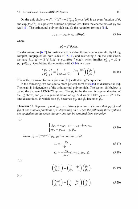
5.2 Recursion and Discrete AKNS-ZS System 111
On the unit circle z = eiθ , V (eiθ )=∑mj=1 2sj cos(jθ) is an even function of θ ,
and exp{V (eiθ )} is a positive function of period 2π . Then the coefficients of pn arereal [11]. The orthogonal polynomials satisfy the recursion formula [11],
pn+1 = zpn + pn+1(0)p∗n, (5.14)
where
p∗n = znpn(z).
The discussions in [6, 7], for instance, are based on this recursion formula. By takingcomplex conjugates on both sides of (5.14), and restricting z on the unit circle,we have pn+1(z) = (1/z)pn(z) + pn+1(0)z−npn(z), which implies p∗
n+1 = p∗n +
pn+1(0)zpn. Combining this equation with (5.14), we have(pn+1p∗n+1
)
=(
z pn+1(0)zpn+1(0) 1
)(pnp∗n
)
. (5.15)
This is the recursion formula given in [11], called Szegö’s equation.In the following, we consider a more general form of (5.15) as discussed in [5].
The result is independent of the orthonormal polynomials. The system (iii) below iscalled the discrete AKNS-ZS system. The pn in the theorem is a generalization ofthe p∗
n above, and pn is a generalization of pn. And we will take γ0 = −1/2 in thelater discussions, in which case pn becomes p∗
n, and pn becomes pn.
Theorem 5.1 Suppose rn and qn are arbitrary functions of n, and that pn(z) andpn(z) are complex functions of z, depending on n. Then the following three systemsare equivalent in the sense that any one can be obtained from any other.
(i){z(pn + vnpn−1)= pn+1 + unpn,
zpn = pn+1 − qnpn,(5.16)
where pn = zn+γ0+1/2pn, γ0 is a constant, and
un = − qn
qn−1, (5.17)
vn = − qn
qn−1(1 − rn−1qn−1). (5.18)
(ii)(pn+1pn+1
)
=(
z qnzrn 1
)(pnpn
)
. (5.19)
(iii)(χn+1χn+1
)
=(η qnrn η−1
)(χnχn
)
. (5.20)

112 5 Densities in Unitary Matrix Models
where η = z1/2, and{χn(η)= z−
n+γ02 pn(z),
χn(η)= zn+γ0
2 pn(z)(5.21)
Proof To derive the system (i) from (ii), we just need to substitute pn = (pn+1 −zpn)/qn (the first equation of (ii)) into the second equation of (ii). After simplifica-tions, the first equation of (i) is obtained. Conversely, the first equation of (i) can beconverted to the second equation of (ii) by using the second equation of (i). So (i)and (ii) are equivalent.
To get (ii) from (iii), we substitute (5.21) into (5.20). Then we have
(pn+1pn+1
)
=(zn+γ0+1
2 0
0 z−n+γ0+1
2
)(z1/2 qnrn z−1/2
)(z−
n+γ02 0
0 zn+γ0
2
)(pnpn
)
,
or(
1 0
0 z(n+γ0+1)+ 12
)(pn+1pn+1
)
=(
z zn+γ0+ 12 qn
zrn zn+γ0+ 12
)(pnpn
)
.
Thus (ii) is obtained. And obviously (iii) can also be derived from (ii). Then thetheorem is proved. �
In the orthonormal case, the original Szegö’s equation is the following recursionformulas
zκn−1Pn−1(z)= κnPn(z)− Pn(0)P∗n (z), (5.22)
κnPn+1(z)= zκn+1Pn(z)+ Pn+1(0)P∗n (z), (5.23)
where Pn(z)= κnpn(z) and κ2n = 1/hn. By eliminating P ∗
n (z), we have
z
(
pn(z)− pn+1(0)
pn(0)
κ2n−1
κ2n
pn−1(z)
)
= pn+1 − pn+1(0)
pn(0)pn(z). (5.24)
Therefore, we have the following relation [12]
hn
hn−1= vn
un= 1 − x2
n. (5.25)
The later discussions will be based on the orthogonal polynomials, in which casethe un and vn are real. But the results in the above theorem is independent of theorthogonal polynomials, that means the un and vn (or rn and qn) can be complexfunctions, in which case the integrable system and the string equation will playan important role because the integrability is not limited to the orthogonal system.The complex function cases can appear in the transition problems as we will see inSect. 6.4 when discussing the power-law divergence. Here, let us give the following

5.3 Lax Pair and String Equation 113
remarks about the more general forms of the string equation, so that as we furtherinvestigate the application problems there is a background to extend the basic mod-els.
The un and vn will be discussed to satisfy the coupled discrete equations (5.35)and (5.36). The set of these coupled equations is the string equation in the unitarymatrix model in terms of the two functions un and vn. By (5.17) and (5.18), thesecoupled equations can be changed to
n
s= −qn + qn−2
qn−1(1 − rn−1qn−1), (5.26)
n
s= − rn + rn−2
rn−1(1 − rn−1qn−1). (5.27)
In particular, if we choose rn−1 = qn−1 = xn (real), then both (5.26) and (5.27)become the string equation in terms of xn,
n
sxn = −(1 − x2
n
)(xn+1 + xn−1). (5.28)
If we choose rn−1 = qn−1(complex conjugate of qn−1), then (5.26) and (5.27) be-come
n
sqn−1 = −(1 − |qn−1|2
)(qn + qn−2). (5.29)
It should be noted that the orthogonality is an important case of the consistencyof the integrable system, but does not cover the general consistency. When the ap-plication problems are not in the scope of the orthogonality, the integrable systemscan extend the model to discuss a wider range of problems.
5.3 Lax Pair and String Equation
5.3.1 Special Potential
By using the orthogonality of the polynomials with the special potential V (z) =s(z+ z−1) (m= 1 case), we will show in this section that the orthogonal polynomi-als pn = pn(z, s) satisfy the following equations:
z(pn + vnpn−1)= pn+1 + unpn, (5.30)
∂pn
∂z=Enpn−1 + Fnpn−2, (5.31)
where
un = −xn+1
xn, (5.32)

114 5 Densities in Unitary Matrix Models
vn = −xn+1
xn
(1 − x2
n
), (5.33)
with xn = pn(0, s), and
En = n, Fn = svnvn−1
unun−1. (5.34)
We are going to show that the consistency condition for (5.30) and (5.30) is thefollowing string equation in terms of un and vn (coupled discrete equations),
n
s= vn + vn
unun−1, (5.35)
n
s= vn
un−1 − vn−1
un − vn+ vn
unun+1
un+1 − vn+1
un − vn. (5.36)
In the following, we first discuss how to derive these equations and explain what theconsistency condition means for the discrete model.
The recursion formula (5.30) is obtained from the Szegö’s equation derived fromthe Christoffel-Darboux formula [11] (Theorem 11.4.2) as discussed in last section,and simplified into the current form [5, 12]. To derive (5.31), write ∂pn/∂z as alinear combination of pn−1,pn−2, . . . , p0:
∂pn
∂z=
n−1∑
k=0
akpk.
Then akhk = 〈 ∂pn∂z,pk〉. It is not hard to see that an−1hn−1 = nhn−1. For k < n− 1,
since on the unit circle (|z| = 1) there is 1/z= z, we have
akhk =∮
∂
∂zpnpke
s(z+1/z) dz
2πiz
= −∮pn
(
− 1
z2
∂
∂zpk − 1
zpk + s
(
1 − 1
z2
)
pk
)
es(z+1/z) dz
2πiz
= shnδn−2,k,
which implies ak = 0 when k < n− 2, and an−2 = shn/hn−2 = Fn, where we haveused the relation hn/hn−1 = vn/un given by (5.25). This gives (5.31).
In the following, we derive the string equation in terms of un and vn by consid-ering the leading coefficient and the second coefficient of pn,z. Equation (5.35) isderived from
〈zpn,z,pn−1〉 = 〈Enzpn−1 + Fnzpn−2,pn−1〉, (5.37)
and (5.36) is obtained from
〈pn+1,z,pn−1〉 = 〈En+1pn + Fn+1pn−1,pn−1〉. (5.38)

5.3 Lax Pair and String Equation 115
It can be seen that, by the recursion formula (5.30), the right hand side of (5.37) isequal to En(un−1 − vn−1)hn−1 +Fnhn−1. For the left hand side of (5.37), considerpn = zn + βnz
n−1 + · · · . Then
z∂pn
∂z= nzn + (n− 1)βnz
n−1 + · · ·= npn − βnpn−1 + · · · .
Equation (5.37) then becomes
−βn = n(un−1 − vn−1)+ svnvn−1
unun−1.
By using the Lemma 5 in [12], we have
vn(un−1 − vn−1)+ vn
un= n
s(un−1 − vn−1)+ vnvn−1
unun−1,
which is (5.35).To compute the left hand side of (5.38), consider pn+1 = zn+1 + βn+1z
n + · · · ,and then
∂pn+1
∂z= (n+ 1)
[
zn + βnzn−1 +
(n
n+ 1βn+1 − βn
)
zn−1 + · · ·]
= (n+ 1)pn + (nβn+1 − (n+ 1)βn)pn−1 + · · · .
Equation (5.38) then becomes
(nβn+1 − (n+ 1)βn
)= svnvn+1
unun+1.
By Lemma 5 in [12] again, we get
−n(un − vn)+ s
(
vn(un−1 − vn−1)+ vn
un
)
= svnvn+1
unun+1.
Thus (5.36) is obtained.The string equation (5.28) in terms of xn can be obtained as follows. Since pn
satisfy the recursion formula, 〈pn,z,pn−1〉 can be calculated by using the recursionformula. We have that by integration by parts
nhn−1 =∮
∂
∂zpnpn−1e
s(z+1/z) dz
2πiz
= −∮pn
[−1
z2
∂pn−1
∂z− 1
zpn−1 + s
(
1 − 1
z2
)
pn−1
]
es(z+1/z) dz
2πiz
= nhn + s(un − vn + un−1 − vn−1)hn.

116 5 Densities in Unitary Matrix Models
Using hn−1/hn = un/vn, we obtain the string equation (5.28). These equations canalso be derived from the Szegö’s equation. Relevant discussions can be found, forexample, in [6, 8]. To avoid the ∗ polynomial p∗
n in the Szegö’s equation, we use therecursion formula (5.30) here.
In the following, we show that (5.30) and (5.31) form a Lax pair for the coupleddiscrete equations (5.35) and (5.36). The results obtained in this section are inde-pendent of the orthonormal polynomials. We only assume that pn(z), as a functionof z, satisfies (5.30) and (5.31), and the functions un and vn satisfy (5.35) and (5.36).
Lemma 5.1 If (5.31) holds, then the recursion formula (5.30) can be changed to
z(Enpn−1 +Xnpn−2)=Enpn + Ynpn−1, (5.39)
where
Xn = Fn + vnEn−1 − un
un−2Fn, (5.40)
Yn = Fn+1 + unEn − vn − un
un−2Fn. (5.41)
Proof Taking ∂/∂z on both sides of (5.30) and applying (5.31), we get
pn + vnpn−1 + z(Enpn−1 + (Fn + vnEn−1)pn−2
)+ zvnFn−1pn−3
=En+1pn + (Fn+1 + unEn)pn−1 + unFnpn−2.
This equation represents a recursion relation for the polynomials pn, which shouldbe consistent with (5.30). To see that, we express vnFn−1zpn−3 − unFnpn−2 interms of pn−1 and zpn−2, such that the equation above comes back to the format of(5.30). In fact, it is not hard to see that
vn
vn−2Fn−1 = un
un−2Fn,
by (5.34). Then we have
vnFn−1zpn−3 − unFnpn−2 = un
un−2Fn(vn−2zpn−3 − un−2pn−2)
= un
un−2Fn(pn−1 − zpn−2).
The recursion formula above then becomes
zEnpn−1 + z(Fn + vnEn−1)pn−2 − zun
un−2Fnpn−2
=Enpn + (Fn+1 + unEn − vn)pn−1 − un
un−2Fnpn−1.
Then this lemma is proved. �

5.3 Lax Pair and String Equation 117
Lemma 5.2 If un and vn satisfy the discrete equations (5.35) and (5.36), then theEn and Fn defined by (5.34) satisfy the relation
Fn+1 + (un − vn)En = Fn + (un−1 − vn−1)En. (5.42)
Proof Since un, vn satisfy (5.35), by multiplying both sides of (5.35) by s(un−1 −vn−1), we have
(un−1 − vn−1)En = s(un−1 − vn−1)vn + svn
un− Fn.
By (5.36), we have
(un − vn)En = s(un−1 − vn−1)vn + svn
un− Fn+1.
Eliminating s(un−1 − vn−1)vn in these two equations, we get (5.42). �
Lemma 5.3 If un and vn satisfy the discrete equations (5.35) and (5.36), then Xn
and Yn defined by (5.40) and (5.41) respectively satisfy
Xn = vn−1En, (5.43)
Yn = un−1En. (5.44)
Proof Write (5.35) in the form
svn
unun−1=En − svn,
and apply it to Fn = svnvn−1unun−1
in (5.40). We then obtain
Xn = vn−1(En − svn)+ vnEn−1 − vn(En−1 − svn−1).
Simplification of this equation yields (5.43).By eliminating Xn in (5.40) and (5.43), we get
un
un−2Fn = Fn + vnEn−1 − vn−1En.
Then by applying this formula to the last term in (5.41), we obtain
Yn = Fn+1 − Fn − vnEn−1 + vn−1En + unEn − vn.
Since En−1 + 1 =En, the last lemma implies (5.44). �
Combining these three lemmas, we have proved the following result.

118 5 Densities in Unitary Matrix Models
Theorem 5.2 The equations
z(pn + vnpn−1)= pn+1 + unpn, (5.45)
∂pn
∂z= npn−1 + s
vn
un
vn−1
un−1pn−2, (5.46)
form a Lax pair for the coupled discrete equations (5.35) and (5.36).
On the unit circle |z| = 1, we can write the above equations of the Lax pair intothe following matrix forms,
Φn+1 = Ln(z)Φn, (5.47)
∂
∂zΦn =An(z)Φn, (5.48)
where Φn(z)= es2 (z+1/z)(z−n/2pn(z), z
n/2pn(z))T ,
Ln =(
z1/2 xn+1z−1/2
xn+1z1/2 z−1/2
)
, (5.49)
An(z)=(
s2 + s
2z2 + n−2sxnxn+12z s(xn+1 − xn
z)z−1
s(xn − xn+1z) − s
2 − s
2z2 − n−2sxnxn+12z
)
, (5.50)
and xn satisfies the string equation
n
sxn = −(1 − x2
n
)(xn+1 + xn−1), (5.51)
with xn ∈ [−1,1]. Note that (5.47) is equivalent to the Szegö’s equation, and it is anequation for Φn(z) here.
Because of the z1/2 term in the Lax pair above, in some literatures, the Laxpair for the string equation is also discussed by using the variable η = z1/2. Basedon Theorem 5.1 and Theorem 5.2, we can get a more general result for the Laxpair for (5.26) and (5.27), which consists of the following two linear systems ofequations [5]
(ψn+1
ψn+1
)
= Ln
(ψn
ψn
)
, (5.52)
∂
∂η
(ψn
ψn
)
= An
(ψn
ψn
)
, (5.53)
where (ψn, ψn)T = e
s2 (η
2+η−2)(χn, χn)T with the (χn, χn) given in last section
(Theorem 5.1),
Ln =(η qnrn η−1
)
, (5.54)

5.3 Lax Pair and String Equation 119
An =(an bncn dn
)
, (5.55)
and
an = sη+ s
η3+ n− γ0 − 2sqnrn−1
η,
bn = 2s
(
qn − qn−1
η2
)
,
cn = 2s
(
rn−1 − rn
η2
)
,
dn = −sη− s
η3− n+ γ0 + 1 − 2sqn−1rn
η.
One can directly check that the consistency condition ∂Ln/∂η = An+1Ln− LnAn isequivalent to (5.26) and (5.27). When rn−1 = qn−1 = xn and γ0 = −1/2, the aboveLax pair (5.52) and (5.53) becomes the Lax pair (5.47) and (5.48). Also, the Laxpairs shown above are consistent with the results obtained in [1, 2], for instance.For the Lax pair of the discrete Painlevé II equation discussed in [2], if we replacen by n + 1, and let ν = 1/2 and κ = s, then their Lax pair becomes the discreteAKNS-ZS system (5.52) and (5.53) with rn−1 = qn−1 = xn and γ0 = −1/2.
As a remark, the coupled equations (5.35) and (5.36) can be converted into thealternate discrete Painlevé II equation [3]. Write (5.35) and (5.36) as follows,
n+ 1
svn = vnvn+1 + vnvn+1
unun+1,
n
s(un − vn) = vn(un−1 − vn−1)+ vn
un− vnvn+1
unun+1.
Adding these two equations, we have
n
sun + vn
s= vn(un−1 − vn−1)+ vn
un+ vnvn+1.
Since nsun = vnun + vn/un−1, the equation above then becomes
(
vn+1 + vn − un + 1
un
)
−(
vn + vn−1 − un−1 + 1
un−1
)
= 1
s,
or
vn+1 + vn − un + 1
un= c0 + n
s,
where c0 = v1 + v0 − u0 + 1/u0. This equation together with (5.35) is the alter-nate string equation in [3]. So the set of the coupled equations (5.35) and (5.36) isequivalent to the alternate string equation.
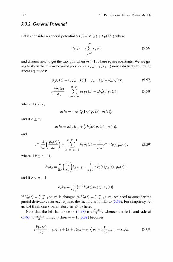
120 5 Densities in Unitary Matrix Models
5.3.2 General Potential
Let us consider a general potential V (z)= V0(z)+ V0(1/z) where
V0(z)= s
m∑
j=1
cj zj , (5.56)
and discuss how to get the Lax pair when m≥ 1, where cj are constants. We are go-ing to show that the orthogonal polynomials pn = pn(z, s) now satisfy the followinglinear equations:
z(pn(z)+ vnpn−1(z)
)= pn+1(z)+ unpn(z); (5.57)
z∂pn(z)
∂z=
n+m∑
k=n−makpk(z)− zV ′
0(z)pn(z), (5.58)
where if k < n,
akhk = −⟨zV ′0(1/z)pn(z),pk(z)
⟩,
and if k ≥ n,
akhk = nhnδk,n + ⟨zV ′0(z)pn(z),pk(z)
⟩;and
z−1 ∂
∂s
(pn(z)
xn
)
=n+m−1∑
k=n−m−1
bkpk(z)− 1
sxnz−1V0(z)pn(z), (5.59)
where if k ≤ n− 1,
bkhk = ∂
∂s
(hn
xn
)
δk,n−1 − 1
sxn
⟨zV0(z)pk(z),pn(z)
⟩,
and if k > n− 1,
bkhk = 1
sxn
⟨z−1V0(z)pn(z),pk(z)
⟩.
If V0(z) =∑mj=1 scj z
j is changed to V0(z) =∑mj=1 sj z
j , we need to consider thepartial derivatives for each sj , and the method is similar to (5.59). For simplicity, letus just think one s parameter s in V0(z) here.
Note that the left hand side of (5.58) is z ∂pn(z)∂z
, whereas the left hand side of
(5.46) is ∂pn(z)∂z
. In fact, when m= 1, (5.58) becomes
z∂pn(z)
∂z= spn+1 + (n+ s(un − vn)
)pn + s
vn
unpn−1 − szpn, (5.60)

5.3 Lax Pair and String Equation 121
with c1 = 1 and s1 = s, which can be changed to (5.46) by using the recursion for-mula and string equation. However, the above equation is obviously not convenientfor discussing the consistency condition. Equation (5.46) can directly and easily pro-vide an example about the consistency condition. The form of (5.58) is so chosen forthe general potential that the matrix form of the Lax pair can be easily formulatedin order to study the eigenvalue density problems. It is left to interested readers toexperience that the equation in the form of (5.46) is not easy to derive the matrixequation. Also, the different forms of the Lax pair are presented here to connect thedifferent results of the Lax pair theory obtained other literatures for a wider impact.
The recursion formula z(pn + vnpn−1) = pn+1 + unpn is still satisfied as dis-cussed before. The z equation (5.58) can be derived by considering
z∂pn(z)
∂z=
n+m∑
k=0
akpk(z)− zV ′0(z)pn(z),
where the term zV ′0(z)pn(z) on the right hand side is so chosen based on the follow-
ing calculations. Using integration by parts and orthogonality for k < n, we have
akhk =∮
∂
∂zpn(z)pk(z)e
V (z) dz
2πi+ ⟨zV ′
0(z)pn,pk⟩
= −∮pn
[
− 1
z2
∂pk(z)
∂z+ (V ′
0(z)+ V ′0(1/z)
)pk(z)
]
zdμ
+ ⟨zV ′0(z)pn(z),pk(z)
⟩
= −⟨zV ′0(1/z)pn(z),pk(z)
⟩,
where dμ = eV (z) dz2πiz . It is not hard to see that ak = 0 when k < n − m since
deg(zV ′0(1/z)pk) < n, where zV ′
0(1/z)pk(z) is a polynomial in z of degree k +m
since |z| = 1. When k ≥ n, ak can be easily found by taking 〈·,pk〉 on both sides ofthe equation.
The s equation can be obtained by considering
z−1 ∂
∂s
(pn
xn
)
=n+m−1∑
k=0
bkpk − 1
sxnz−1V0(z)pn(z).
The left side of the equation is a polynomial in z of degree n − 1, and the factor1sxn
z−1 on the right hand side is chosen based on the following calculations. Whenk > n− 1, taking 〈·,pk〉 on both sides of this equation, we get the formula for bk .When k ≤ n− 1, bj can be found by using the product rule and orthogonality of thepolynomials. Still taking 〈·,pk〉 on both sides of this equation, we have
bkhk =∮z−1 ∂
∂s
(pn
xn
)
pkdμ+ 1
sxn
⟨z−1V0(z)pn(z),pk(z)
⟩

122 5 Densities in Unitary Matrix Models
= ∂
∂s
∮z−1pn
xnpkdμ−
∮z−1pn
xn
∂pk
∂sdμ
−∮z−1pn
xnpk
1
sV (z)dμ+ 1
sxn
⟨z−1V0(z)pn(z),pk(z)
⟩
= ∂
∂s
(hn
xn
)
δk,n−1 − 1
sxn
∮pnz
−1V0(1/z)pkdμ
= ∂
∂s
(hn
xn
)
δk,n−1 − 1
sxn
⟨zV0(z)pk(z),pn(z)
⟩.
It can be seen that when k < n−m− 1 there are bk = 0.We have shown that the orthogonal polynomials pn satisfy the three linear equa-
tions simultaneously. We are interested in finding the consistency conditions forthese linear equations. If we choose xn as the function variable, the consistencycondition for (5.57) and (5.58) is the string equation hierarchy, and the consistencycondition for (5.57) and (5.59) is the Toda lattice for the unitary matrix models. Theconsistency condition for (5.58) and (5.59) is the continuum Painlevé III or V hier-archy, which is a more complicated case, and we will discuss the special cases inSect. C.3.
First, the string equation hierarchy has the following general formula [6, 7]
n(hn − hn−1)= ⟨V ′(z)pn(z),pn−1(z)⟩. (5.61)
In fact, by integration by parts, we have
nhn−1 =∮pn,zpn−1e
V (z) dz
2πiz
= −∮pn
(−1
z2
∂pn−1
∂z− 1
zpn−1 + V ′(z)pn−1
)
dμ
= nhn − ⟨V ′(z)pn(z),pn−1(z)⟩.
When m= 1, V ′(z)= s1(1 − z−2), (5.61) is (5.28).When m= 2, V ′(z)= s1(1 − z−2)+ 2s2(z− z−3) with sj = scj , (5.61) becomes
n(hn−1 − hn)
= s1⟨z2pn−1(z),pn(z)
⟩− 2s2⟨zpn(z),pn−1(z)
⟩+ 2s2⟨z3pn−1(z),pn(z)
⟩.
By repeatedly using the recursion formula, we can find
zpn = pn+1 + unpn − vn(pn + un−1pn−1 − vn−1zpn−2),
z2pn−1 = pn+1 + unpn + (un−1 − vn−1 − vn)(pn + un−1pn−1 − vn−1zpn−2)
− vn−1z(un−2pn−2 − vn−2zpn−3),
z3pn−1 = pn+2 + un+1pn+1
+ (un − vn + un−1 − vn−1 − vn+1)(pn+1 + unpn − vnzpn−1)

5.3 Lax Pair and String Equation 123
+ (un−1 − vn−1 − vn)z(un−1pn−1 − vn−1zpn−2)
− vn−1z2(un−2pn−2 − vn−2zpn−3).
The equation can be written as
n(hn−1 − hn) = s1(un − vn + un−1 − vn−1)hn + 2s2vn(un−1 − vn−1)hn−1
+ 2s2[(un − vn + un−1 − vn−1 − vn+1)(un − vn)
+ (un−1 − vn−1 − vn)(un−1 − vn−1)− vn−1(un−2 − vn−2)]hn.
And it can be further simplified to
nxn
1 − x2n
= −s1(xn+1 + xn−1)+ 2s2xn(xn+1 + xn−1)2
− 2s2xn+2(1 − x2
n+1
)− 2s2xn−2(1 − x2
n−1
), (5.62)
by using (5.32) and (5.33). This is (3.7) in [1].The consistency conditions can be also formulated in terms of the un and
vn functions. As in the m = 1 case, we need to consider 〈pn,z(z),pn−2(z)〉 and〈zpn,z(z),pn−1(z)〉. Let pn = zn + βnz
n−1 + · · · . Then we have⟨pn,z(z),pn−2(z)
⟩ = [n(βn − βn−1)− βn]hn−2, (5.63)
⟨zpn,z(z),pn−1(z)
⟩ = −βnhn−1. (5.64)
The βn satisfy the following relations
βn − βn−1 = −(un−1 − vn−1),
βnhn−1 = −⟨zV ′(z)pn(z),pn−1(z)⟩.
The first relation holds because pn− zpn−1 = (βn −βn−1)zn−1 +· · · = −un−1pn−1
+ vn−1zpn−2. For the second relation, consider J = 〈zpn(z),pn−1(z)〉. By integra-tion by parts, we have
J = 1
s
∮pnpn−1e
V (z)−sz desz
2πi
= −1
s
∮ [∂pn
∂zpn−1 + pn
−1
z2
∂pn−1
∂z+ pnpn−1
(V ′(z)− s
)]
eV (z)dz
2πi
= −1
s− βnhn−1 − 1
s
⟨zV ′(z)pn(z),pn−1(z)
⟩+ ⟨zpn(z),pn−1(z)⟩.
Thus we get βnhn−1 = −〈zV ′(z)pn(z),pn−1(z)〉.By the s equation (5.59), we can get the following Toda lattice,
x′n(hn − hn−1)= xn
s
⟨V (z)
(pn(z)− zpn−1(z)
),pn(z)
⟩. (5.65)

124 5 Densities in Unitary Matrix Models
In fact, the left hand side of (5.59) is a polynomial in z of degree n− 1. If we takethe inner product 〈·,pn−1(z)〉 on both sides of (5.59), then after some simplificationsthere is
x′n(hn − hn−1)= xnh
′n − xn
s
⟨zV (z)pn−1(z),pn(z)
⟩.
By the definition of hn, we have
h′n = 1
s
⟨V (z)pn(z),pn(z)
⟩.
By eliminating h′n in these two equations above, we get (5.65).
5.4 Densities Reduced from the Lax Pair
Now, let us come back to the general potential V (z) = V0(z) + V0(z−1), where
V0(z) =∑mj=1 sj z
j . We want to obtained the expected analytic function ω(z) forsolving the eigenvalue density problem by using the coefficient matrix An in theLax pair based on the discussions in the last two sections using the similar methodwe have done in Chap. 2.
Based on (5.58) obtained in last section
z∂pn(z)
∂z=
m∑
j=−man+jpn+j (z)− zV ′
0(z)pn(z), (5.66)
we have the following matrix equation on the unit circle
z∂
∂z
(pnpn
)
=m∑
j=−man+j σ3
(pn+jpn+j
)
−(zV ′
0(z) 00 zV ′
0(z−1)
)(pnpn
)
, (5.67)
where σ3 =diag(1,−1) and V0′ = ∂
∂zV0. The recursion formula (5.47) with rn−1 =
qn−1 = xn and γ0 = −1/2 or the Szegö’s equation implies
(pn+1
zn+1pn+1
)
= Tn+1LnT−1n
(pnznpn
)
, (5.68)
where
Ln =(z− un+1 zvn+1
1 0
)
, Tn =(
0 11
xn+1
−zxn+1
)
. (5.69)
Let Φn(z)= e12 (V0(z)+V0(1/z))(z−n/2pn(z), z
n/2pn(z))T . Then there is
∂
∂zΦn(z)=An(z)Φn(z), (5.70)

5.4 Densities Reduced from the Lax Pair 125
where
zσ3An(z) =m∑
j=1
an+j(
1 00 z−j
)
Tn+j Ln+j−1 · · · LnT −1n
+m∑
j=1
an−j(
1 00 zj
)
Tn−j Ln−j · · · Ln−1T−1n
+(
an − n
2
)
I − 1
2z(V ′
0(z)− V ′0
(z−1))I. (5.71)
The eigenvalue density ρ(θ) will be obtained from the Lax pair in the unitarymatrix models following a process, roughly expressed as
1
nπ
√detAn(z)dz∼ σ(z)dz= ρ(θ)dθ, (5.72)
for z= eiθ on the complement of the arc cuts in the unit circle. We also need
1
n
√−detAn(z)∼ ω(z), (5.73)
where z = 0, z = ∞ and z is outside the cuts, to analyze the asymptotics as z → 0or z→ ∞. Note that the eigenvalues are now on the complement of the cuts, and itis easy to see that
σ(z)= 1
πiω(z), (5.74)
for z on the complement of the cuts. The details are much more complicated than theHermitian matrix models. In order to get similar results as in the Hermitian modelsdiscussed in Chap. 2, we need to apply the different forms of the recursion formuladiscussed in Sect. 5.2 such that the determinant of the matrix in the correspondingCayley-Hamilton theorem is independent of z, and the factor (−1)n or the similarfactors will play an important role in the matrix transformations. The factor (−1)n isfundamental in the reduction of the density models for the unitary matrix models. Inthe Hermitian matrix models, a fundamental consideration is about the index changefrom n to n + 1, say, and the eigenvalues are distributed on the cut(s) on the realline. In the unitary matrix models, we typically need to consider the factor (−1)n
for constructing the eigenvalue densities which are defined on the complement ofthe cut(s) in the unit circle. Interested readers can first try the case m = 2 or 3.To reduce the pages of the book and pay more attention to the phase transitionproblems, the details for the reduction and factorization processes are omitted here.In the following, we introduce some simple examples for readers to see the key stepsto obtain the density formulas. The general formulations are not discussed here sincethis book focus on the application problems by considering the special models. Theterminologies, strong and weak couplings, are used in the following discussions justfor reader’s convenience to associating with the strong and weak couplings in theGross-Witten model. Here, we only talk about the mathematical formulations.

126 5 Densities in Unitary Matrix Models
5.4.1 Strong Couplings: General Case
The strong coupling densities are derived by assuming un and vn both approach tov as n→ ∞, so that (tr Ln)2 − 4 det Ln becomes a complete square and the formulaof the density finally does not have square root. In this case, xn will approach to0, Ln±k will be replaced by Ln, and Tn±j will be replaced by diag(1, (−v)∓j )Tn.Also by the orthogonality of the polynomials, there are an±j = jsj and an = n.The
√−detAn can be rescaled and reduced to ω(z) as we worked before for theHermitian matrix models. The details can be discussed based on the Lax pair. Theexplicit formula for ω(z) is
zω(z)= 1
2
m∑
j=1
jgj(1 − (−vz)−j )(zj − (−v)j ), (5.75)
which can be further simplified to
zω(z)= 1
2
m∑
j=1
jgj(zj + z−j
)+ 1
2, (5.76)
if the parameters satisfy the conditions
m∑
j=1
jgj((−v)j + (−v)−j )+ 1 = 0. (5.77)
Then, using the equivalent relation, ρ(θ)dθ = σ(z)dz, where σ(z) = ω(z)/(πi),the density formula can be obtained either in the z space or θ space.
5.4.2 Weak Couplings: One-Cut Cases
The weak coupling densities on one interval can be derived by assuming un ap-proach to 1 and vn approach to v as n → ∞ by referring the Gross-Witten weakcoupling density model. The square root factor in the density can be formulated bythe matrix
L(1) =(z− 1 zv
1 0
)
, (5.78)
which gives (tr L(1))2 − 4 det L(1) = (z − 1)2 + 4vz. In this case, Ln±k will be re-placed by the L(1), and Tn±j will be replaced by Tn in the reduction to get ω(z).Here, let us just talk about some special cases.
When U(z)= g1(z+ z−1), there is
zω(z)= 1
2g1(1 + z−1)
√(z− 1)2 + 4vz, (5.79)

5.4 Densities Reduced from the Lax Pair 127
subject to the condition 2g1v = 1 with g1 ≥ 1/2, which is corresponding to theGross-Witten weak coupling density discussed before.
When U(z)=∑mj=1 gj (z
j + z−j ) for m= 2 or 3, there is
zω(z)= 1
2f (z)
(1 + z−1)
√(z− 1)2 + 4vz, (5.80)
where
f (z)= g1 − 4g2v+ 3g3(1 − 4v+ 6v2)+ [2g2 − 6g3v]
(z+ z−1)+ 3g3
(z2 + z−2),
(5.81)subject to the condition
g1v + 2g2(2v − 3v2)+ 3g3
(3v(1 − v)(1 − 3v)+ v3)= 1
2. (5.82)
The ω(z) function so defined has the following asymptotics
zω(z)= 1
2z(U ′
0(z)−U ′0
(z−1))+ 1
2+O
((z1/2 + z−1/2)−2)
, (5.83)
as |z1/2 + z−1/2| → ∞, where U0(z)=∑3j=1 gj z
j . These results can be applied tostudy the transition problems to be discussed in the next chapter. The density func-tion also needs to be non-negative when the variable is transformed into the θ space,while in the z space the “density” could be complex function. The z space is usedfor the mathematical calculation such as the asymptotics for an easier computationusing the complex integrals.
The ω(z) functions obtained above are defined in the outside of the cut Ω = {z=eiθ | cos(θ/2)≤ √
1 − v, θ ∈ [−π,π]} in the complex plane. The eigenvalue densityρ(θ) is defined by ρ(θ)dθ = σ(z)dz, where σ(z)= ω(z)/πi is defined on the Ω ={|z| = 1}�Ω on the unit circle, where Ω is the complement of Ω in the unit circle,which will be discussed in detail in next chapter. As a remark, the function y(z)=zω(z)− 1
2z(U′0(z)−U ′
0(z−1))− 1
2 , satisfies the following relations, y(z) is analytic
when z ∈ C�{Ω ∪ {0} ∪ {∞}}; y(z)|Ω+ + y(z)|
Ω− = −z(U ′0(z) − U ′
0(z−1)) − 1;
y(z) → 0 as z → 0 or ∞. These properties are needed in discussing the densitymodels.
5.4.3 Weak Coupling: Two-Cut Case
Consider the potential
U(z)= g1(z+ z−1)+ g2
(z2 + z−2), (5.84)

128 5 Densities in Unitary Matrix Models
or U(z)=U0(z)+U0(z−1) where U0(z)= g1z+ g2z
2. The density formula can beobtained by using the matrix
L(2) =(z− u(1) zv(1)
1 0
)(z− u(2) zv(2)
1 0
)
. (5.85)
Let us first consider the case when u(1) = u(2) = 1, g1 = 0 and v(1) + v(2) = 2.Also there is a relation v(1)v(2) = 1 − 1
4g2coming from the expansion of ω to
meet with the potential, which is different from the m = 1 or 3 cases becausewhen the degree of the potential polynomial is different, the number of the termsin the expansion changes. In this case, the ω function is given by zω(z) = g2(1 +z−2)
√Λ2 − 4 det L(2), where Λ= tr L(2) = z2 + 1 and det L(2) = z2v(1)v(2), or
zω(z)= g2(z+ z−1)
√(z− z−1
)2 + g−12 , g2 ≥ 1
4. (5.86)
The ω(z) satisfies
zω(z)= 1
2z(U ′
0(z)−U ′0
(z−1))+ 1
2+O
((z+ z−1)−2)
, (5.87)
as |z+ z−1| → ∞ including z → ∞ and z → 0, where U0(z)= g2z2. Note that in
the expansion, we need first to change the term z− z−1 in the square root to z+ z−1
before the expansion calculations since we consider large z+ z−1. This is importantfor all of the weak coupling models considered in Chaps. 5 and 6.
The critical point g2 = 1/4 is not corresponding to the parameter bifurcation likewe did before, because when g2 = 1/4 there is v(1)v(2) = 0, but v(1) + v(2) = 2.That means at the critical point we can not have v(1) = v(2) as we worked beforeif we want to reduce L(2) to (L(1))2. If we consider u(1) = u(2) = i and v(1) +v(2) = 2i. The relation between v(1)v(2) and g2 becomes v(1)v(2) = −1 − 1
4g2. The
critical point becomes g2 = −1/4 which still leads to v(1)v(2) = 0. If we considerthe general case with g1 = 0, the condition v(1)v(2) = 0 at the critical point is stillthere. So the transition model for the second degree potential is different from theGross-Witten transition model. The physical background for this phenomenon is notclear yet. Mathematically, the odd terms and even terms in the potential functionusually lead to different properties. We will see in Sect. 6.4 that everything worksfine except that it is not a parameter bifurcation case at the critical point.
For the ω(z) defined by (5.86), the analytic function y(z)= zω(z)− 12z(U
′0(z)−
U ′0(z
−1))− 12 , defined in the outside of the cut Ω = {z = eiθ || cos θ | ≤
√1 − 1
4g2},
has the properties that y(z) is analytic when z ∈ C�{Ω ∪ {0} ∪ {∞}}, y(z)|Ω+ +
y(z)|Ω− = −z(U ′
0(z)−U ′0(z
−1))− 1, and y(z)→ 0 as z→ 0 or ∞.

5.4 Densities Reduced from the Lax Pair 129
5.4.4 Weak Coupling: Three-Cut Case
Consider the potential
U(z)= g3(z3 + z−3), (5.88)
or U(z) = U0(z) + U0(z−1) where U0(z) = g3z
3. The interesting result in thismodel is the critical point Tc = 1/gc3 = 6, which is discussed in [22] for the four-dimensional quantum chromodynamics to create the string model.
Denote
L(3) =(z− 1 zv(1)
1 0
)(z− 1 zv(2)
1 0
)(z− 1 zv(3)
1 0
)
, (5.89)
and define
zω(z)= 3
2g3(1 + z−3)
√
Λ2 − 4 det L(3), (5.90)
with v(1) + v(2) + v(3) = 3. Then Λ = tr L(3) = z3 − 1, and det L(3) =−z3v(1)v(2)v(3). If 6g3v
(1)v(2)v(3) = 1, then
zω(z)= 3
2g3(z3/2 + z−3/2)
√(z3/2 − z−3/2
)2 + 2
3g−1
3 , g3 ≥ 1
6, (5.91)
which implies the asymptotics
zω(z)= 1
2z(U ′
0(z)−U ′0
(z−1))+ 1
2+O
((z3/2 + z−3/2)−2)
, (5.92)
as |z3/2 + z−3/2| → ∞.If g3 = 1/6, then zω(z) = 1
4 (z3/2 + z−3/2)2. In this case, we can choose v(1) =
v(2) = v(3) = 1, and then L(3) = (L(1))3, that means this is a parameter bifurcationcase. For the strong density with this potential discussed before in this section, wecan choose v = 1 at the critical point to have g3 = 1/6, and the zω(z) meets withthe critical case obtained for the weak coupling. It is seen that the transition modelin this case is caused by the parameter bifurcation in the sense that v becomes v(1),v(2) and v(3), which extends the Gross-Witten transition model.
Also, the function y(z) = zω(z) − 12z(U
′0(z) − U ′
0(z−1)) − 1
2 , satisfies the fol-
lowing properties. The y(z) is analytic when z ∈ C�{Ω ∪ {0} ∪ {∞}}; y(z)|Ω+ +
y(z)|Ω− = −z(U ′
0(z) − U ′0(z
−1)) − 1; y(z) → 0 as z → 0 or ∞, where Ω is the
union of the three cuts | cos(3θ/2)| ≤√
1 − 16g3
for z= eiθ on the unit circle at the
points z= −1, z= eiπ/3 and z= e−iπ/3.

130 5 Densities in Unitary Matrix Models
References
1. Cresswell, C., Joshi, N.: The discrete first, second and thirty-fourth Painlevé hierarchies.J. Phys. A 32, 655–669 (1999)
2. Grammaticos, B., Nijhoff, F.W., Papageorgiou, V., Ramani, A., Satsuma, J.: Linearization andsolutions of the discrete Painlevé III equation. Phys. Lett. A 185, 446–452 (1994)
3. Grammaticos, B., Ohta, Y., Ramani, A., Sakai, H.: Degenerate through coalescence of theq-Painlevé VI equation. J. Phys. A 31, 3545–3558 (1998)
4. Gross, D.J., Witten, E.: Possible third-order phase transition in the large-N lattice gauge the-ory. Phys. Rev. D 21, 446–453 (1980)
5. McLeod, J.B., Wang, C.B.: Discrete integrable systems associated with the unitary matrixmodel. Anal. Appl. 2, 101–127 (2004)
6. Periwal, V., Shevitz, D.: Unitary-matrix models as exactly solvable string theories. Phys. Rev.Lett. 64, 1326–1329 (1990)
7. Periwal, V., Shevitz, D.: Exactly solvable unitary matrix models: multicritical potentials andcorrelations. Nucl. Phys. B 344, 731–746 (1990)
8. Rossi, P., Campostrini, M., Vicari, E.: The large-N expansion of unitary-matrix models. Phys.Rep. 302, 143–209 (1998)
9. Simon, B.: Orthogonal Polynomials on the Unit Circle, Vol. 1: Classical Theory. AMS Collo-quium Series. AMS, Providence (2005)
10. Simon, B.: Orthogonal Polynomials on the Unit Circle, Vol. 2: Spectral Theory. AMS Collo-quium Series. AMS, Providence (2005)
11. Szegö, G.: Orthogonal Polynomials, 4th edn. American Mathematical Society ColloquiumPublications, vol. 23. AMS, Providence (1975)
12. Wang, C.B.: Orthonormal polynomials on the unit circle and spatially discrete Painlevé IIequation. J. Phys. A 32, 7207–7217 (1999)

Chapter 6Transitions in the Unitary Matrix Models
The first-, second- and third-order phase transitions, or discontinuities, in the unitarymatrix models will be discussed in this chapter. The Gross-Witten third-order phasetransition is described in association with the string equation in the unitary ma-trix model, and it will be generalized by considering the higher degree potentials.The critical phenomena (second-order divergences) and third-order divergences arediscussed similarly to the critical phenomenon in the planar diagram model, but adifferent Toda lattice and string equation will be applied here by using the doublescaling method. The discontinuous property in the first-order transition model ofthe Hermitian matrix model discussed before will recur in the first-order transitionmodel of the unitary matrix model, indicating a common mathematical backgroundbehind the first-order discontinuities. The purpose of this chapter is to further con-firm that the string equation method can be widely applied to study phase transi-tion problems in matrix models, and that the expansion method based on the stringequations can work efficiently to find the power-law divergences considered in thetransition problems.
6.1 Large-N Models and Partition Function
For the potential V (z) = s(z + z−1), we have discussed the linear equations sat-isfied by the orthogonal polynomials pn = pn(z, s) on the unit circle in the n andz directions in last chapter. In the z direction, we have obtained in Sect. 5.3 that∂∂zΦn =An(z)Φn, where
An(z)=(
s2 + s
2z2 + n−2sxnxn+12z s(xn+1 − xn
z)z−1
s(xn − xn+1z) − s
2 − s
2z2 − n−2sxnxn+12z
)
, (6.1)
and xn satisfies the string equation
n
sxn = −(1 − x2
n
)(xn+1 + xn−1), (6.2)
C.B. Wang, Application of Integrable Systems to Phase Transitions,DOI 10.1007/978-3-642-38565-0_6, © Springer-Verlag Berlin Heidelberg 2013
131

132 6 Transitions in the Unitary Matrix Models
Fig. 6.1 Three X curves inthe unitary model
with xn ∈ [−1,1]. Then, we have that
−z2
s2detAn = 1
4
(z+ z−1 + T
)2 − X
4, (6.3)
where T = n/s, and
X = (x′n)
2 − T 2x2n
1 − x2n
+ 4x2n, (6.4)
with ′ = d/ds.In Sect. D.2, it is discussed that the following values of X (see Fig. 6.1) are
the singular points of the hypergeometric-type differential equation satisfied by theelliptic integrals,
X =
⎧⎪⎨
⎪⎩
T 2 + 2, 0 < T ≤ 1/2,
(T − 2)2, 1/2 ≤ T ≤ 2,
0, T ≥ 2.
(6.5)
Here, the T values are divided in the three regions for studying the transition prob-lems. Based on the reduction formulation 1
nπ
√detAndz= σ(z)dz, we will consider
the transition problems for the following phases in the next two sections,
σ(z)=
⎧⎪⎪⎨
⎪⎪⎩
12T πiz
√(z+ z−1 + T )2 − T 2 − 2, 0 < T ≤ 1/2,
12T πiz
√(z+ z−1 + 2)(z+ z−1 + 2T − 2), 1/2 ≤ T ≤ 2,
12T πiz (z+ z−1 + T ), T ≥ 2.
(6.6)
The derivatives of the partition function Zn = n!h0h1 · · ·hn−1 [13, 14] in the sdirection are important for discussing the phase transitions, which are similar to theresults obtained in the Hermitian matrix models. For the hn’s, by the discussions inSect. 5.3, there are
h′0 = −2x1h0, h′
n = −2xnxn+1hn, n≥ 1, (6.7)
where ′ = d/ds. Then, there is
d
dslnZn = −2x1 − 2
n−1∑
j=1
xjxj+1. (6.8)

6.1 Large-N Models and Partition Function 133
We will discuss later that the xn’s satisfy the following Toda lattice,
x′1 = (1 − x2
1
)(x2 − 1), x′
n = (1 − x2n
)(xn+1 − xn−1), n≥ 2. (6.9)
Therefore, we have
d2
ds2lnZn = 2
(1 − x2
n
)(1 − xn−1xn+1), (6.10)
for n≥ 2. Equation (6.10) implies that the second-order derivative of the free energywill be continuous if we study the reduced models using the bifurcation transitionmethod as discussed in the Hermitian matrix models. But the term xn−1xn+1 in(6.10) will cause a second-order divergence in the s direction to be explained inSect. 6.3.
Since the s direction is so important for the transition problems, we need to gothrough the details of the system in this direction in order to show how the second-order divergence is caused. We will see that this divergence is because the contin-uum Painlevé III equation is involved. The discussions for the equations satisfied bythe xn or the un and vn in the s direction can be found, for example, in [4, 5, 10]. Aswe have experienced in Chap. 4, the Lax pairs are the basic models for investigatingthe divergent behaviors. Here, we want to setup the Lax pairs for the Toda latticeand the continuum Painlevé III or V equation. Let us consider the linear equation inthe s direction in order to get the Lax pair for the Toda lattice or continuum Painlevéequation. It has been discussed in Sect. 5.3 that for the potential V (z)= s(z+ z−1),the orthogonal polynomials pn(z) satisfy the following equation in the s equation,
z−1 ∂
∂s
pn
xn=
n−1∑
k=n−2
bkpk, (6.11)
where
bkhk = ∂
∂s
(hn
xn
)
δk,n−1 − 1
xn
∮z2pkpne
s(z+1/z) dz
2πiz, (6.12)
for k = n− 2 and n− 1. Therefore, we have obtained
∂
∂s
pn
xn= bn−1zpn−1 + bn−2zpn−2, (6.13)
where
bn−1 = 1
hn−1
∂
∂s
(hn
xn
)
− hn
hn−1xn(un − vn + un−1 − vn−1), (6.14)
bn−2 = − hn
hn−2xn. (6.15)
One of the consistency conditions for (6.13) and the recursion formula can befound by comparing the leading coefficients on both sides of (6.13). Since the for-mula for bn−1 above involves ∂hn/∂s, we also need the formula of ∂hn/∂s given
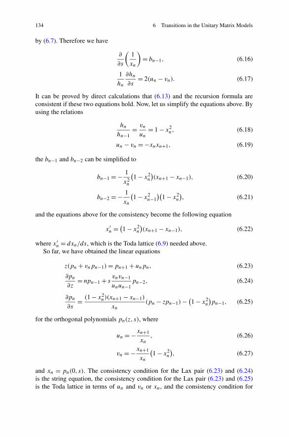
134 6 Transitions in the Unitary Matrix Models
by (6.7). Therefore we have
∂
∂s
(1
xn
)
= bn−1, (6.16)
1
hn
∂hn
∂s= 2(un − vn). (6.17)
It can be proved by direct calculations that (6.13) and the recursion formula areconsistent if these two equations hold. Now, let us simplify the equations above. Byusing the relations
hn
hn−1= vn
un= 1 − x2
n, (6.18)
un − vn = −xnxn+1, (6.19)
the bn−1 and bn−2 can be simplified to
bn−1 = − 1
x2n
(1 − x2
n
)(xn+1 − xn−1), (6.20)
bn−2 = − 1
xn
(1 − x2
n−1
)(1 − x2
n
), (6.21)
and the equations above for the consistency become the following equation
x′n = (1 − x2
n
)(xn+1 − xn−1), (6.22)
where x′n = dxn/ds, which is the Toda lattice (6.9) needed above.
So far, we have obtained the linear equations
z(pn + vnpn−1)= pn+1 + unpn, (6.23)
∂pn
∂z= npn−1 + s
vnvn−1
unun−1pn−2, (6.24)
∂pn
∂s= (1 − x2
n)(xn+1 − xn−1)
xn(pn − zpn−1)− (1 − x2
n
)pn−1, (6.25)
for the orthogonal polynomials pn(z, s), where
un = −xn+1
xn, (6.26)
vn = −xn+1
xn
(1 − x2
n
), (6.27)
and xn = pn(0, s). The consistency condition for the Lax pair (6.23) and (6.24)is the string equation, the consistency condition for the Lax pair (6.23) and (6.25)is the Toda lattice in terms of un and vn or xn, and the consistency condition for
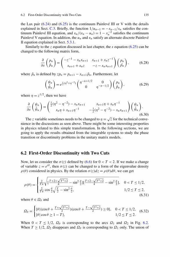
6.2 First-Order Discontinuity with Two Cuts 135
the Lax pair (6.24) and (6.25) is the continuum Painlevé III or V with the detailsexplained in Sect. C.3. Briefly, the function 1/un−1 = −xn−1/xn satisfies the con-tinuum Painlevé III equation, and vn/(vn − un) = 1 − x−2
n satisfies the continuumPainlevé V equation. In addition, the un and vn satisfy an alternate discrete PainlevéII equation explained in Sect. 5.3.1.
Similarly to the z equation discussed in last chapter, the s equation (6.25) can bechanged to the following matrix form,
∂
∂s
(pnpn
)
=(
−z−1 − xnxn+1 xn+1 + xnz−1
xn+1 + xnz −z− xnxn+1
)(pnpn
)
, (6.28)
where pn is defined by zpn = pn+1 − xn+1pn. Furthermore, let(ψn
ψn
)
= es2 (η
2+η−2)
(η−n+1/2 0
0 η−n−1/2
)(pnpn
)
, (6.29)
where η = z1/2, then we have
∂
∂s
(ψn
ψn
)
=(
12 (η
2 − η−2)− xnxn+1 xn+1η+ xnη−1
xnη+ xn+1η−1 − 1
2 (η2 − η−2)− xnxn+1
)(ψn
ψn
)
.
(6.30)The z variable sometimes needs to be changed to η = √
z for the technical conve-nience in the discussions as seen above. There might be some interesting propertiesin physics related to this simple transformation. In the following sections, we aregoing to apply the results obtained from the integrable systems to study the phasetransition or discontinuity problems in the unitary matrix models.
6.2 First-Order Discontinuity with Two Cuts
Now, let us consider the σ(z) defined by (6.6) for 0 < T < 2. If we make a changeof variable z = eiθ , then σ(z) can be changed to a form of the eigenvalue densityρ(θ) considered in physics. By the relation σ(z)dz= ρ(θ)dθ , we can get
ρ(θ)=
⎧⎪⎨
⎪⎩
2T π
√
[T+2+√T 2+2
4 − sin2 θ2 ][T+2−
√T 2+2
4 − sin2 θ2 ], 0 < T ≤ 1/2,
2T π
cos θ2
√T2 − sin2 θ
2 , 1/2 ≤ T ≤ 2,(6.31)
where θ ∈Ωθ and
Ωθ ={
{θ |(cos θ + T+√T 2+2
2 )(cos θ + T−√T 2+2
2 )≥ 0}, 0 < T ≤ 1/2,
{θ | cos θ ≥ 1 − T }, 1/2 ≤ T ≤ 2.(6.32)
When 0 < T ≤ 1/2, Ωθ is corresponding to the arcs Ω1 and Ω2 in Fig. 6.2.When T ≥ 1/2, Ω2 disappears and Ωθ is corresponding to Ω1 only. The union of

136 6 Transitions in the Unitary Matrix Models
Fig. 6.2 Cuts (thick arcs) andeigenvalue range (thin arcs)
Ω =Ω1 ∪Ω2 and Ω = Ω1 ∪ Ω2 is the unit circle, so Ω is the compliment of Ω inthe unit circle. When 0 < T < 1/2, the ρ function does not satisfy the non-negativitycondition since the density function on the arc across z = −1 (see Fig. 6.2) is neg-ative. This is a case like the model discussed in Sect. 4.1.2. This negative-positivemodel can be changed to a non-negative model by constructing the density on twocoupled arcs passing the point z = 1, similar to the discussion in Sect. 4.1.2. Weare not going to discuss the details here since we want to keep the discussions interms of ρ for consistency. As T is increased to 1/2, the two cuts on the unit circlemerge together at the point z = −1, that will cause a first-order discontinuity to bediscussed in the following.
Define the ω function as
ω(z)={
12T z
√(z+ z−1 + T )2 − T 2 − 2, 0 < T ≤ 1/2,
12T z
√(z+ z−1 + 2)(z+ z−1 + 2T − 2), 1/2 ≤ T ≤ 2,
(6.33)
for z in the complex plane outside the cut(s) Ω and the points z = 0 and ∞, withthe following asymptotics
zω(z)={
12T (z+ z−1)+ 1
2 +O((z+ z−1 + T )−1), 0 < T ≤ 1/2,1
2T (z+ z−1)+ 12 +O((z+ z−1 + 2)−1), 1/2 ≤ T ≤ 2,
(6.34)
as z→ 0 or z→ ∞, where U(z)= T −1(z+ z−1). Note that for this special poten-tial, there is U(z) = z(U ′
0(z)− U ′0(1/z)) where U0(z) = T −1z. This could cause a
confusion that one may still search the analytic function zω(z) with the asymptotics12U(z) for the higher degree potentials. But the analytic function zω(z) generallyneed to have an asymptotics with the leading term 1
2z(U′0(z)−U ′
0(1/z)) in order tosatisfy the variational equation discussed in Sect. 5.1 because of the two essentialsingular points z = 0 and ∞. Also, the two O terms in the above expansions aredifferent.
Lemma 6.1 The σ(z) defined by (6.6) for 0 < T < 2 satisfies
(P)∫
Ω
σ(ζ )
z− ζdζ = −1
2U ′(z)+ 1
2z, (6.35)
for an inner point z in Ω , where∫Ωσ(z)dz= 1.

6.2 First-Order Discontinuity with Two Cuts 137
Proof Let C+ and C− be the closed counterclockwise outside and inside edges ofthe unit circle respectively, and C∗ = C+ ∪C−. By Cauchy theorem, there is
{∫
C∗−∫
|z|=δ−∫
|z|=R
}(
ω(z)− 1
2zU(z)
)
dz= 0,
which implies the following by the asymptotics at 0 and ∞,∫
C∗
(
ω(z)− 1
2zU(z)
)
dz→∫
|z|=Rdz
2z+∫
|z|=δdz
2z= 2πi,
as δ → 0 and R → ∞. Since∫C∗ U(z)dz/z = 0 and ω(z)|
Ω+ + ω(z)|Ω− = 0, we
have∫Ω
1πiω(z)|Ωdz= 1. Therefore
∫Ωσ(z)dσ = ∫
Ω1πiω(z)|Ωdz= 1.
Consider a point z in Ω . Choose a small ε > 0 and make a small circle of radiusε with center z. Let the “semicircle” inside of the unit circle |z| = 1 be γ−
ε , and the“semicircle” outside the unit circle be γ+
ε . Remove the small arc around z (|z| =1) enclosed by the ε circle from the unit circle. The remaining arc is denoted asC(ε). As ε → 0, C(ε) becomes the unit circle. All the closed contours are orientedcounterclockwise. Then by Cauchy theorem, there is
(∫
C+(ε)∪γ+ε
+∫
C−(ε)∪γ−ε
)(
ζω(ζ )− 1
2T
(ζ + ζ−1)− 1
2
)dζ
ζ − z= 0,
where γ±ε are given in the above discussion. Since the small semicircles γ+
ε and γ−ε
have opposite directions around the point z, there is(∫
γ+ε
+∫
γ−ε
)(
ζω(ζ )− 1
2T
(ζ + ζ−1)− 1
2
)dζ
ζ − z→ 0,
as ε → 0. Because the integrals of ζω(ζ ) along the inside and outside edges of thecuts are canceled, there is(∫
C+(ε)+∫
C−(ε)
)
ζω(ζ )dζ
ζ − z= 2
∫
Ω(ε)
ζω(ζ )dζ
ζ − z→ 2(P)
∫
Ω
ζω(ζ )dζ
ζ − z,
as ε → 0, where Ω(ε) is the Ω without the small arc at the point z. Also, we have
1
πi
∫
C(ε)
(1
2T
(ζ + ζ−1)+ 1
2
)dζ
ζ − z
= 1
2πi
∫
C(ε)∪γ−ε
1
ζ − zdζ + 1
2T πi
∫
C(ε)∪γ−ε
ζ
ζ − zdζ
+ 1
2T πi
∫
C(ε)∪γ+ε
ζ−1
ζ − zdζ
− 1
2πi
∫
γ−ε
1
ζ − zdζ − 1
2T πi
∫
γ−ε
ζ
ζ − zdζ − 1
2T πi
∫
γ+ε
ζ−1
ζ − zdζ
→ 1
2+ 1
2T
(z− z−1)= 1
2zU ′(z)+ 1
2,

138 6 Transitions in the Unitary Matrix Models
as ε → 0, where the three integrals alongC(ε)∪γ−ε or C(ε)∪γ+
ε vanish. Therefore,we get
(P)∫
Ω
ζσ(ζ )
ζ − zdζ = 1
2zU ′(z)+ 1
2,
and then (6.35) is proved. �
Lemma 6.2 For an inner point z of Ω , there is∫
Ω
σ(ζ )
z− ζdζ = −1
2U ′(z)+ 1
2z+ω(z), (6.36)
for 0 < T < 2.
Proof If we keep using the notations in the proof of last lemma, then for z in Ω
there is(∫
C+(ε)∪γ+ε
+∫
C−(ε)∪γ−ε
)ζω(ζ )− 1
2U(ζ )− 12
ζ − zdζ = 0,
based on the asymptotics at ζ = 0 and ζ = ∞. Further, since ω has opposite signson the two edges of the cut(s), there are∫
C+(ε)∪C−(ε)
ζω(ζ )
ζ − zdζ +
∫
γ+ε ∪γ−
ε
ζω(ζ )
ζ − zdζ → 2
∫
Ω
ζω(ζ )
ζ − zdζ + 2πizω(z),
and{
2∫
C(ε)
+∫
γ+ε ∪γ−
ε
} 12U(ζ )+ 1
2
ζ − zdζ
= 2∫
C(ε)
12T (ζ + ζ−1)+ 1
2
ζ − zdζ
= −2∫
γ−ε
12T ζ + 1
2
ζ − zdζ − 2
∫
γ+ε
12T ζ
−1
ζ − zdζ → 2πi
(1
2T
(z− z−1)+ 1
2
)
,
as ε → 0. Then, we get the following∫
Ω
ζσ(ζ )
ζ − zdζ = 1
2zU ′(z)− zω(z)+ 1
2, (6.37)
and this lemma is proved. �
Now, consider
E = −∫
Ω
U(z)σ (z)dz−∫
Ω
∫
Ω
ln |z− ζ |σ(z)σ (ζ )dzdζ. (6.38)
We will see a first-order discontinuity at the critical point T = 1/2.

6.2 First-Order Discontinuity with Two Cuts 139
Lemma 6.3
dE
dT={
1T 2
∫Ω(z+ z−1)σ (z)dz− 2
∫Ω1
ω(η)dη ddT
∫Ω2
σ(z)dz, 0 < T ≤ 1/2,1T 2
∫Ω(z+ z−1)σ (z)dz, 1/2 ≤ T < 2,
(6.39)where Ω =Ω1 ∪Ω2 with 1 ∈Ω1 and −1 ∈Ω2, and Ω1 is the cut between Ω1 andΩ2, where all arcs are oriented counterclockwise.
Proof When 0 < T ≤ 1/2, we have
dE
dT= −
∫
Ω
dU(z)
dTσ(z)dz
− 2
(∫
Ω1
+∫
Ω2
)(∫
Ω
ln |z− ζ |σ(ζ )dζ + 1
2U(z)
)dσ(z)
dTdz.
By the lemmas above, for z ∈Ω1 there is∫
Ω
ln |z− ζ |σ(ζ )dζ + 1
2U(z)=
∫
Ω
ln |z0 − ζ |σ(ζ )dζ + 1
2U(z0),
where z0 is the start point of Ω1 (Fig. 6.2), and for z ∈Ω2 there is∫
Ω
ln |z− ζ |σ(ζ )dζ + 1
2U(z)=
∫
Ω
ln |z0 − ζ |σ(ζ )dζ + 1
2U(z0)+
∫
Ω1
ω(z)dz.
Then the result is true by using ddT
∫Ω1∪Ω2
σ(z)dz= ddT
1 = 0. When 1/2 ≤ T < 2,
the (· · · ) part in the second term on the right hand side of the formula dEdT
above isconstant because Ω is now a connected arc, which can be moved to the outside ofthe integral leading the entire integral to vanish. �
Lemma 6.4 As T → 1/2 − 0, there are the following expansions,
T = 1
2− 3
4ε2, (6.40)
z± = −1 ± iε+ · · · , (6.41)
where z± are the end points of Ω2 defined by z± + z−1± + T + √T 2 + 2 = 0.
Proof Substituting the expansions z = −1 + c1ε + c2ε2 + · · · and T = 1
2 + T1ε +T2ε
2 into the equation z + z−1 + T + √T 2 + 2 = 0, we can get the expansion re-
sults. �
Theorem 6.1 The E function given by (6.38) has discontinuous first-order deriva-tive at T = 1/2,
E′(1/2 + 0)−E′(1/2 − 0)= 2 + 1√3
ln(2 − √3), (6.42)
where ′ = d/dT .

140 6 Transitions in the Unitary Matrix Models
Proof According to (6.38), we only need to consider
I0 ≡ 2∫
Ω1
ω(z)dzd
dT
∫
Ω2
σ(z)dz. (6.43)
By Lemma 6.4, if we make a transformation z = −eiεφ around z = −1, then as Tapproaches to 1/2, there is
σ(z)dz∼√
3
πε2√
1 − φ2dφ,
where φ is from −1 to 1, that implies
d
dT
∫
Ω2
σ(z)dz→ − 2√3.
Also, as T → 1/2 − 0, we have∫
Ω1
ω(z)dz→ 2i∫ π
π/3cos
θ
2
√
1 − 1
4sin2 θ
2dθ = −
√3
2− 1
4ln(2 − √
3),
which implies E′(1/2 + 0)−E′(1/2 − 0)= limε→0 I0 = 2 + 1√3
ln(2 − √3), since
∫Ω(z+ z−1)σ (z)dz is continuous. �
We have seen the exact same term 1√3
ln(2 − √3) in the model discussed in
Sect. 4.1.2, which could be related to an interesting physical problem.
6.3 Double Scaling Associated with Gross-Witten Transition
Consider the σ(z) defined by (6.6) for T > 1/2. By the transformation σ(z)dz =ρ(θ)dθ with z= eiθ , there are the following weak and strong coupling densities [3]
ρ(θ)=⎧⎨
⎩
2T π
cos θ2
√T2 − sin2 θ
2 , 1/2 ≤ T ≤ 2,1
2π (1 + 2T
cos θ), T ≥ 2,(6.44)
where θ ∈Ωθ and
Ωθ ={
{θ || sin θ2 | ≤ √
T/2, |θ | ≤ π}, 1/2 ≤ T ≤ 2,
{θ ||θ | ≤ π}, T ≥ 2.(6.45)
Then the free energy
E = − 2
T
∫
Ωθ
cos(θ)ρ(θ)dθ −∫
Ωθ
∫
Ωθ
ln
∣∣∣∣sin
θ − θ ′
2
∣∣∣∣ρ(θ)ρ
(θ ′)dθdθ ′
+ 1
2π
∫ π
−πln
∣∣∣∣sin
θ
2
∣∣∣∣dθ (6.46)

6.3 Double Scaling Associated with Gross-Witten Transition 141
has the following explicit formulas [3],
E ={− 2
T− 1
2 ln T2 + 3
4 , T ≤ 2,
− 1T 2 , T ≥ 2.
(6.47)
It can be checked that the free energy has continuous first- and second-order deriva-tives, and its third-order derivative is discontinuous at T = 2. This is a brief descrip-tion of the well known Gross-Witten third-order phase transition found in 1980,see [3].
In the following, we are going to discuss the reduction of the eigenvalue densitiesρ from the coefficient matrix An given by (6.1) in the Lax pair. The determinant ofAn can be written as [11]
√detAn(z)
= 1
i
√(s
2+ s
2z2+ n− 2sxnxn+1
2z
)2
+ s2
z
(
xn − xn+1
z
)(
xn+1 − xn
z
)
.
(6.48)
Consider n/s = T and un = −xn+1/xn. Then the string equation (6.2) becomesT/(1 − x2
n)= un + 1/un−1, or asymptotically as n and s → ∞,
un ∼[
T
2(1 − x2n)
+√(
T
2(1 − x2n)
)2
− 1
]−1
.
If T = 2(1 − x2n)(≤ 2), then un ∼ 1, or xn+1 ∼ −xn ∼ xn−1, that implies
1
nπ
√detAn(z)dz∼ 2
πTcos
θ
2
√T
2− sin2 θ
2dθ, (6.49)
where z= eiθ . If T > 2, then un < 1, or xn → 0, that implies
1
nπ
√detAn(z)dz∼ 1
2π
(
1 + 2
Tcos θ
)
dθ. (6.50)
These results are corresponding to the weak and strong coupling densities (6.44)obtained in [3].
Now, let us consider a critical phenomenon, a second-order discontinuity relatedbut differing from the third-order discontinuity talked above. The string equation(6.2) can be reduced to
gv = 1
2, (6.51)
by taking xn−1 ∼ −xn ∼ xn+1 according to the above reduction, where g = s/n =T −1 and 1 − x2
n ∼ v. Consider the ε expansions
g = 1
2+ ε, (6.52)

142 6 Transitions in the Unitary Matrix Models
and
v = 1
1 + 2ε= 1 − 2ε+O
(ε2). (6.53)
Then, there is x2n ∼ 2ε. In the s direction, as s → n/2+0 we have xn =O(
√s − n
2 ),
and then
dxn/ds =O(|s − n/2|−1/2). (6.54)
Come back to the formula d2
ds2 logZn = 2(1 − x2n)(1 − xn−1xn+1) obtained in
Sect. 6.3. By the discussion in Sect. C.3, we have
xn−1xn+1 = (nxn)2/s2 − (x′
n)2
4(1 − x2n)
2, (6.55)
where ′ = d/ds, that implies
d2
ds2logZn = 2
(1 − x2
n
)− (nxn)2/s2 − (x′
n)2
2(1 − x2n)
. (6.56)
According to the discussion above, we then have the critical phenomenon
d2Fn
ds2=O
((dxn/ds)
2)=O(|s − n/2|−1), (6.57)
with the critical point s = n/2, where Fn = − logZn which is different from thefree energy E = − lim 1
n2 logZn discussed above. The formula of Fn is close tothe free energy in statistical mechanics [18]. Also, the original physical model [3]in the unitary matrix model involves the parameter n in the discussion of the freeenergy, which means the Fn considered here has a physical background. Since xn =O(
√ε) and g = 1/2 + ε > 1/2, the transition in the above critical phenomenon
is between the strong coupling phase in the Gross-Witten transition model and thephase 1
nπ
√detAn(z)dz which is on the same side T = g−1 < 2 of the weak coupling
phase in the Gross-Witten transition model, with a weaker coupling structure sincethere are four roots for detAn(z)= 0 in the complex plane. One can use the methoddiscussed in Sect. 4.3.1 to get (6.56) by the free energy formula in terms of thedensity based on the linear equations in the s direction discussed in Sect. 6.1. Thedetails are omitted here since the discussion in Sect. 6.1 to derive (6.10) is sufficient.
The above discussions can be summarized as follows. If we consider the localvariable s, then the second-order derivative of logZn is divergent, d2Fn
ds2 = O(|s −n/2|−1) as s → n/2 + 0. If we consider the temperature variable T = n/s with thereduction xn−1 ∼ −xn ∼ xn+1 then we get a third-order discontinuity with
d3E
dg3= −4v1
dε
dg
(1 +O(ε)
)→ 8, (6.58)

6.3 Double Scaling Associated with Gross-Witten Transition 143
as g → 1/2 + 0 and d3E/dg3 = 0 as g → 1/2 − 0. The method can be extended tohigher degree potentials to get other critical phenomena to be discussed in the latersections. These results are all based on the string equations to create the relationsbetween the parameters in the model so that the critical phenomena can be derivedby using the ε-expansions.
The model for this critical phenomenon has a closer structure to the originaldiscrete integrable system since we only supply the condition (6.51) to the integrablemodel (6.56). Note that this critical phenomenon model is not included in the phasesdiscussed in Sect. 6.1 where the singular values of X are from the hypergeometric-type differential equation. It is interesting to investigate what has happened at thecritical point T = 2, such as where the consistency or the integrability has beentransited to. In the following, we use the double scaling method to discuss that thediscrete integrable system can be reduced to the continuum integrable system toexplain the transition of the integrability.
Let us first consider the string equation in terms of un and vn
n
s= vn + vn
unun−1, (6.59)
n
s= vn
un−1 − vn−1
un − vn+ vn
unun+1
un+1 − vn+1
un − vn. (6.60)
discussed in Sect. 5.3. It is given in last chapter that (6.59) and (6.60) are the con-sistency conditions for the Lax pair
z(pn + vnpn−1)= pn+1 + unpn, (6.61)
∂pn
∂z= npn−1 + s
vnvn−1
unun−1pn−2. (6.62)
We are going to apply the double scalings to the un and vn functions to show thescaling properties around n/s = 2 based on the discussions in [10, 13, 14, 17]. Thedouble scaling is also used in other literatures for different problems. Here, we applythe double scaling method to discuss the phase transition problem.
Denote dn = vn − un. Equations (6.59) and (6.60) then become
n
s= (un + dn)
(
1 + 1
unun−1
)
, (6.63)
n
s= (un + dn)
(dn−1
dn+ 1
unun+1
dn+1
dn
)
. (6.64)
In this section, we show that as n and s → ∞, if we make the following doublescaling in large-N asymptotics,
2s
n= 1 + c0x/n
β, (6.65)
un = 1 + c1
nα
ux
u+ · · · , (6.66)
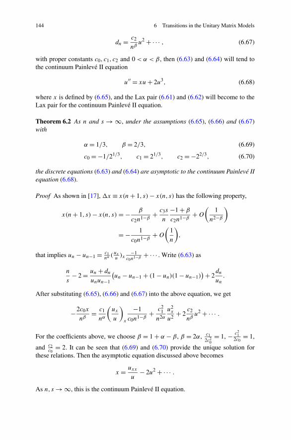
144 6 Transitions in the Unitary Matrix Models
dn = c2
nβu2 + · · · , (6.67)
with proper constants c0, c1, c2 and 0 < α < β , then (6.63) and (6.64) will tend tothe continuum Painlevé II equation
u′′ = xu+ 2u3, (6.68)
where x is defined by (6.65), and the Lax pair (6.61) and (6.62) will become to theLax pair for the continuum Painlevé II equation.
Theorem 6.2 As n and s → ∞, under the assumptions (6.65), (6.66) and (6.67)with
α = 1/3, β = 2/3, (6.69)
c0 = −1/21/3, c1 = 21/3, c2 = −22/3, (6.70)
the discrete equations (6.63) and (6.64) are asymptotic to the continuum Painlevé IIequation (6.68).
Proof As shown in [17], !x ≡ x(n+ 1, s)− x(n, s) has the following property,
x(n+ 1, s)− x(n, s) = − β
c2n1−β + c3s
n
−1 + β
c2n1−β +O
(1
n2−β
)
= − 1
c0n1−β +O
(1
n
)
,
that implies un − un−1 = c1nα(uxu)x
−1c0n
1−β + · · · . Write (6.63) as
n
s− 2 = un + dn
unun−1
(un − un−1 + (1 − un)(1 − un−1)
)+ 2dn
un.
After substituting (6.65), (6.66) and (6.67) into the above equation, we get
−2c0x
nβ= c1
nα
(ux
u
)
x
−1
c0n1−β + c21
n2α
u2x
u2+ 2
c2
nβu2 + · · · .
For the coefficients above, we choose β = 1 + α − β , β = 2α, c12c2
0= 1, − c2
12c0
= 1,
and c2c0
= 2. It can be seen that (6.69) and (6.70) provide the unique solution forthese relations. Then the asymptotic equation discussed above becomes
x = uxx
u− 2u2 + · · · .
As n, s → ∞, this is the continuum Painlevé II equation.

6.3 Double Scaling Associated with Gross-Witten Transition 145
Also, (6.64) can be written as
n
s− 2 = un + dn
unun−1
dn−1
dn
(un − un−1 + (1 − un)(1 − un−1)
)
+ 2dn
un+ un + dn
unun−1
(dn+1
dn− dn−1
dn
)
,
which also approaches the continuum Painlevé II equation by noting that dn+1 −dn−1 =O( 1
n1+β ) given by (6.67). �
The above discussions imply that
x2n = 1 − (1 − x2
n
)= un − vn
un=O
(2s
n− 1
)
, (6.71)
as n and s are large. This asymptotics is consistent with the result discussed before.To complete the discussion for the cause of the transition at the critical point interms of double scaling, we also need to consider the double scaling limit of the Laxpair. It is known that the continuum Painlevé II equation u′′ = xu+ 2u3 has the Laxpair [6]
Ψx =(−iλ iu
−iu iλ
)
Ψ,
Ψλ =(−4iλ2 − 2iu2 − ix 4iλu− 2ux
−4iλu− 2ux 4iλ2 + 2iu2 + ix
)
Ψ,
where Ψ = (ψ1,ψ2)T . Eliminating ψ2 we get
ψxx = ux
uψx +
(iλux
u− λ2
)
ψ + u2ψ,
ψλ =(
−ix − 2iu2 − 2λuxu
)
ψ +(
4λ+ 2iux
u
)
ψx,
where ψ =ψ1. Let ψ = eixλ+ 4i3 λ
3φ. We then have
φxx =(
u2 + 2iλuxu
)
φ +(
−2iλ+ ux
u
)
φx, (6.72)
φλ = 2i
(
−x − u2 + 2iλuxu
)
φ + 2i
(
−2iλ+ ux
u
)
φx, (6.73)
where the first equation is a different version of the Schrödinger equation. This isthe Lax pair in scalar form for the continuum Painlevé II equation. We are goingto show in the following that the Lax pair of the coupled discrete equation can beasymptotically reduced to these two equations.

146 6 Transitions in the Unitary Matrix Models
To discuss the asymptotics of the Lax pair (6.61) and (6.62), let
pn(z)= (−1)nφn(z). (6.74)
This trivial transformation is important. It will be seen that the function that tendsto φ is φn, not pn. In fact, φnesz → φ. Therefore (6.61), in terms of φn, becomes
−z(φn − (un + dn)φn−1)= φn+1 − unφn. (6.75)
Also it is not hard to see that (6.62) becomes
φn,z = −nφn−1 + s
(
1 + dn
un
)(
1 + dn−1
un−1
)
φn−2.
To derive (6.73), we need to express φn,z in terms of φn and φn+1. Notice thatvn = un + dn, and
vn−1φn−2 = 1
zφn + φn−1 − un−1
zφn−1,
n= s
(
vn + vn
unun−1
)
,
so that from the equation for φn,z above we have
φn,z = −nφn−1 + svn
unun−1
(1
zφn + φn−1 − un−1
zφn−1
)
= −svnφn−1 + svn
unun−1zφn − svn
unzφn−1.
Apply the recursion formula
vnφn−1 = φn + 1
zφn+1 − un
zφn
to the above equation. After some simplifications, we obtain
1
sφn,z + φn = −
(
z+ 1
un
)1
z2(φn+1 − φn)+ (un − 1)
(
z+ 1
un
)1
z2φn
+ vn − un
unun−1zφn + un − un−1
unun−1zφn. (6.76)
Now we are ready to prove the following theorem.
Theorem 6.3 With the assumptions (6.65), (6.66) and (6.67) as n, s → ∞, and
z= −1 + 24/3i
n1/3λ, (6.77)

6.3 Double Scaling Associated with Gross-Witten Transition 147
φnesz = φ(λ, x)+ o(1), (6.78)
the equations (6.75) and (6.76) are asymptotic to (6.72) and (6.73) respectively.
Proof In order to get (6.72), write (6.75) as
φn+1 + φn−1 − 2φn = (un + dn − 1)(φn − φn−1)− (1 + z)(φn − (un + dn)φn−1
)
− dnφn.
Since
(φn − φn−1)esz = φx!x + · · · ,
(φn+1 + φn−1 − 2φn)esz = φxx!x
2 + · · · ,the equation above becomes
φxx1
c20n
2/3= c1
n1/3
ux
uφx
−1
c0n1/3+ 2iλ
c0n1/3
(
φx−1
c0n1/3− c1
n1/3
ux
uφ
)
− c2
n2/3u2φ
+ o(n−2/3),
or
φxx = −c0c1ux
uφx − 2iλφx − c0c12iλ
ux
uφ − c2
0c2u2φ + o(1),
where o(1) represents the remaining terms which tend to zero as n, s → ∞. There-fore, if we take n, s → ∞, (6.72) is obtained.
Substituting the asymptotic formulas into (6.76), we have
2
n2/3
1
24/3iφλ = −21/3
n2/3
(
24/3iλ− 21/3 ux
u
)
φx + 21/3
n2/3
ux
u
(
24/3iλ− 21/3 ux
u
)
φ
+ 22/3
n2/3u2φ − 22/3
n2/3
(ux
u
)
x
φ.
After some simplifications, we obtain
φλ = 2i
[
u2 −(ux
u
)
x
+ 2iλux
u−(ux
u
)2]
φ − 2i
(
2iλ− ux
u
)
φx + o(1).
As n, s → ∞, it is reduced to (6.73). �
If we refer Fig. 6.2 to study this scaling deformation, the point z in (6.77) iscorresponding to the point z0 in Fig. 6.2, but not the points z±, and there is noΩ2 in this case. This means the integrability is transited at z = −1 as the arc Ω =Ω1 is becoming large until to the unit circle. The vertical direction in z = −1 +24/3i
n1/3 λ is consistent with the transition process shown in the Gross-Witten model.

148 6 Transitions in the Unitary Matrix Models
One can experience that the s equation can not join with the double scaling aboveto become an equation in the new integrable system. This property indicates thatthe parameters or variable n, s and z in the system perform different roles in thereduction of the transition models, and the models can be distinguished accordingto which parameter direction(s) the integrable system is deformed along to form atransition model.
If the integrable system is reduced in the n direction, then at the critical pointT = 2, there is a third-order transition, which is the Gross-Witten transition model.If the integrable system is reduced in the s direction, then the parameter n is keptin the density and free energy, and the transition is of second-order, in which casethere is
dg
d lnv= 0, (6.79)
at the critical point g = 1/2, according to the strong coupling condition given inSect. 5.4.2. If the integrable system is reduced in both n and s directions with the nparameter controlling the free energy and the s parameter controlling the X variablein the density model, then we get a first-order discontinuity. Note that the weakand strong coupling densities in the Gross-Witten transition model can be obtainedseparately from the string equation and the Toda lattice. The first case is associatedwith the n and z equations, and the second case is related to the z and s equationsas shown by (6.4) and (6.5) in association with the discussions in Sect. D.2. Thereduction conditions in these two cases can not be applied together. For example, ifwe apply 1 − x2
n = T/2 to the equation X = (T − 2)2, then we get x′n = 0, which is
a contradiction. In the first case, the xn’s are more like “particles” as the reductionxn+1 ∼ −xn ∼ xn−1 has shown. In the second case, the xn’s perform as “waves”since the xn satisfies a differential equation for the elliptic function in the s direction.These two performances indicate a duality of the xn in the Gross-Witten model,which is a new property derived from the integrable system and deserves furtherinvestigations in physics.
6.4 Third-Order Transitions for the Multi-cut Cases
In this section, we discuss the transition model with the potential
U(z)= 1
T
(zm + z−m
), (6.80)
where m is an positive integer. Define the ω function by
zω(z)= m
2T
(zm + z−m
)+ 1
2, (6.81)
for T ≥ 2m where z is in the complex plane. And define the ω function by
zω(z)= m
2T
(zm/2 + z−m/2)
√(zm/2 + z−m/2
)2 + 2
m(T − 2m), (6.82)

6.4 Third-Order Transitions for the Multi-cut Cases 149
Fig. 6.3 Cuts (thick arcs)and eigenvalue range (thinarcs) for m= 3
for T ≤ 2m with z ∈C�Ω where Ω is the union of cuts on the unit circle,
Ω = {z= eiθ || cos(mθ/2)| ≤√1 − (T /2m), |θ | ≤ π}. (6.83)
Figure 6.3 shows the three cuts Ω and the complement of Ω in the unit circle (threearcs Ω) for m = 3. In this case, we will see that critical point is T = 6 which ispossibly another expected transition remarked by Gross and Witten in [3] (Sect. IV)when they discuss an approximation for the four-dimensional QCD U(N) gaugetheory. According to [3], the physical model is expected to be constructed basedon the analysis of the critical value [2, 15] and the bounded properties of the one-plaquette Wilson loop. As a remark, when m= 1 there is only one cut (arc) passingthrough the point z = −1. When m = 2, there are two cuts (arcs) passing throughz= i and z= −i respectively.
In both cases discussed above (T ≤ 2m and T ≥ 2m), we have
zω(z)= m
2T
(zm + z−m
)+ 1
2+O
((zm/2 + z−m/2)−2)
, (6.84)
as |zm/2 + z−m/2| → ∞. Define σ(z) by
σ(z)= 1
πiω(z), (6.85)
on Ω = {|z| = 1} for T ≥ 2m and on Ω = {z||z| = 1}�Ω for T ≤ 2m. It is not hard
to get∫Ωσ(z)dz= 1. Since σ(zei
2πm )d(zei
2πm )= σ(z)dz, we have
∫
Ωj
σ (z)dz= 1
m, (6.86)
where Ωj ’s are the disjoint arcs of Ω such that Ω =⋃mj=1Ωj . This property will
be applied to simplify the calculation of the free energy. As before, σ(z) can bechanged to ρ(θ) by
ρ(θ)dθ = σ(z)dz, (6.87)
where z= eiθ . The square root in (6.82) takes alternative positive and negative signson the cuts such that ρ(θ) is non-negative for z ∈ Ω . The polynomial outside thesquare root can balance the negative sign from the square root. In fact, if we make

150 6 Transitions in the Unitary Matrix Models
the change of variables zm/2 + z−m/2 = 2 cosφ = 2x, then these density models arelike the densities in the Hermitian matrix models. More discussions will be given atthe end of this section.
Let us now first consider the variational equation satisfied by the eigenvalue den-sities for T ≥ 2m which is a case similar to the strong coupling model discussed inSect. 5.1 for T ≥ 2 when m = 1. We will see that these unitary matrix models canbe discussed similarly. Choose a point z on the unit circle and a small ε > 0, thenmake a circle of radius ε with center z. Denote the “semicircle” inside the unit circle|z| = 1 as γ−
ε , and the “semicircle” outside the unit circle as γ+ε . Remove the small
arc around z enclosed by the ε circle from the unit circle. The remaining big arc isdenoted as Ω(ε). As ε → 0, Ω(ε) becomes the unit circle, and
∫Ω(ε)
→ (P)∫Ω
to beused in the following discussions. Denote Ω− =Ω(ε)∪ γ−
ε and Ω+ =Ω(ε)∪ γ+ε .
All the closed contours are oriented counterclockwise. Then, we have for T ≥ 2m,
1
πi
∫
Ω(ε)
ζω(ζ )
ζ − zdζ
= 1
2πi
∫
Ω−1
ζ − zdζ + m
2T πi
∫
Ω−ζm
ζ − zdζ + m
2T πi
∫
Ω+ζ−m
ζ − zdζ
− 1
2πi
∫
γ−ε
1
ζ − zdζ − m
2T πi
∫
γ−ε
ζm
ζ − zdζ − m
2T πi
∫
γ+ε
ζ−m
ζ − zdζ
→ 1
2+ m
2T
(zm − z−m
)= 1
2zU ′(z)+ 1
2,
as ε → 0, where the three integrals along Ω+ or Ω− vanish. Based on this result,we have the following lemma.
Lemma 6.5 The σ(z) defined by (6.85) satisfies
(P)∫
Ω
ζσ(ζ )
ζ − zdζ = 1
2zU ′(z)+ 1
2, (6.88)
where |z| = 1 for T ≥ 2m, and z is an inner point of Ω for T ≤ 2m.
Proof We have proved the T ≥ 2m case above. When T ≤ 2m, since z is an innerpoint of Ω , we can choose a small ε > 0 and make a small circle of radius ε withcenter z to remove a small arc from Ω . Let Ω±
0 (ε) be reduced from the unit circle|ζ | = 1 by removing the small arc at z and changing the portions at the cuts tothe inside and outside edges respectively, both oriented counterclockwise. Then byCauchy theorem, there is
(∫
Ω+0 (ε)∪γ+
ε
+∫
Ω−0 (ε)∪γ−
ε
)(
ζω(ζ )− m
2T
(ζm + ζ−m)− 1
2
)dζ
ζ − z= 0,

6.4 Third-Order Transitions for the Multi-cut Cases 151
where γ±ε are given in the above discussion. Since the small semicircles γ+
ε and γ−ε
have opposite directions around the point z, there is(∫
γ+ε
+∫
γ−ε
)(
ζω(ζ )− m
2T
(ζm + ζ−m)− 1
2
)dζ
ζ − z→ 0,
as ε → 0. Because the integrals of ζω(ζ ) along the inside and outside edges of thecuts Ω are canceled, there is(∫
Ω+0 (ε)
+∫
Ω−0 (ε)
)
ζω(ζ )dζ
ζ − z= 2
∫
Ω(ε)
ζω(ζ )dζ
ζ − z→ 2(P)
∫
Ω
ζω(ζ )dζ
ζ − z,
as ε → 0, where Ω(ε) is the Ω without the small arc at the point z. Also, we have
1
πi
(∫
Ω+0 (ε)
+∫
Ω−0 (ε)
)(m
2T
(ζm + ζ−m)+ 1
2
)dζ
ζ − z→ zU ′(z)+ 1,
as ε → 0. Then the lemma is proved. �
The γ±ε (ε) play different roles in the two cases, T ≥ 2m and T ≤ 2m discussed
above. When T ≤ 2m, we need to use Ω±0 (ε) so that the properties of the ω(z) at
the cuts can be applied. In the following, we first convert the formula in the abovelemma into a new form so that it can be applied to calculate the free energy function.
Theorem 6.4 The σ(z) defined by (6.85) satisfies
(P)∫
Ω
σ(ζ )
z− ζdζ = −1
2U ′(z)+ 1
2z, (6.89)
for both T ≤ 2m and T ≥ 2m where z is an inner point of Ω .
At the critical point T = 2m, both the weak and strong densities become ρc(θ)=1π
cos2 mθ2 , for θ ∈ [−π,π]. To discuss the transition at this critical point, consider
the free energy function
E =∫
Ω
(−U(z))σ(z)dz−∫
Ω
∫
Ω
ln |z− ζ |σ(z)σ (ζ )dzdζ. (6.90)
When T ≥ 2m, the theorem above implies that
E = − 1
2πT
∫ π
−πcos(mθ)
(
1 + 2m
Tcos(mθ)
)
dθ
− 1
2π
∫ π
−πln |2 sin θ/2|
(
1 + 2m
Tcos(mθ)
)
dθ − 1
T,
that gives
E = − m
T 2, T ≥ 2m. (6.91)

152 6 Transitions in the Unitary Matrix Models
When T ≤ 2m, the eigenvalues z are distributed on m arcs, and the integral overeach arc is equal to 1/m according to (6.86), so that d
dT
∫Ωj
σ (z)dz = 0 for each
arc Ωj . Then, we have dEdT
= − ∫Ω
dU(z)dT
σ (z)dz. In fact, if we denote the zj as thestart point of each arc Ωj , and take integral from zj to z for an inner point z in Ωj
on both sides of (6.89), then there is∫
Ω
ln |ζ − z|σ(ζ )dζ −∫
Ω
ln |ζ − zj |σ(ζ )dζ = −1
2
(U(z)−U(zj )
), z ∈Ωj,
for j = 1, . . . ,m. Multiplying dσ(z)dz
on both sides and taking integral from zj to z,
and using the result∫Ωj
ddTσ (z)dz= 0 obtained above, we get
∫
Ωj
(∫
Ω
ln |ζ − z|σ(ζ )dζ)dσ(z)
dTdz= −1
2
∫
Ωj
U(z)dσ (z)
dTdz,
which implies∫
Ω
(∫
Ω
ln |ζ − z|σ(ζ )dζ)dσ(z)
dTdz= −1
2
∫
Ω
U(z)dσ (z)
dTdz. (6.92)
Because
dE
dT= −
∫
Ω
dU(z)
dTσ(z)dz−
∫
Ω
U(z)dσ (z)
dTdz
− 2∫
Ω
∫
Ω
ln |ζ − z|σ(ζ )dσ (z)dT
dζdz,
we then get dEdT
= − ∫Ω
dU(z)dT
σ (z)dz for T < 2m, or
dE
dT= m
2T 3
∫
Ω+0 ∪Ω−
0
(zm + z−m
)(zm/2 + z−m/2)
×√(zm/2 + z−m/2
)2 + 2
m(T − 2m)
dz
2πiz, (6.93)
where Ω±0 are the outside and inside edges respectively of the unit circle according
to the cuts Ω . Both Ω−0 and Ω−
0 are oriented counterclockwise so that the integrals∫Ω+
0and
∫Ω−
0are canceled at the cuts resulting 1
2 (∫Ω+
0+ ∫
Ω−0)= ∫
Ω, that is why
∫Ω
is changed to 12
∫Ω+
0 ∪Ω−0
in the above. The integrand above is asymptotic to
z2m + z−2m + T
m
(zm + z−m
)− T
2m2(T − 4m)+ o(1),
as z→ ∞ or z→ 0. Then there is
dE
dT= 2
T 2− 1
2mT, T ≤ 2m, (6.94)

6.4 Third-Order Transitions for the Multi-cut Cases 153
by changing∫Ω+
0 (ε)to∫|z|=R , and
∫Ω−
0 (ε)to∫|z|=δ with R → ∞ and δ → 0. Since
E(2m)= − 14m , we have
E = − 2
T− 1
2mln
T
2m+ 3
4m, T ≤ 2m. (6.95)
Theorem 6.5 The free energy
E ={
− 2T
− 12m ln T
2m + 34m, T ≤ 2m,
− m
T 2 , T ≥ 2m,(6.96)
has continuous first- and second-order derivatives, and discontinuous third-orderderivative,
d3
dT 3E(2m−)= 10
(2m)4<
12
(2m)4= d3
dT 3E(2m+). (6.97)
The above result shows that the coefficient of ln T2m changes as m changes. If this
property can be related to other transition problems, it would be interesting. As stud-ied in the transition models in statistical mechanics, such as the Kosterlitz-Thoulesstransition for the two dimensional XY model, the coefficient of the logarithmic termin the free energy is always important.
The density models discussed above are created on the unit circle. We can changethese models to the real line, for example, for the m= 2 case. If we make a bilineartransformation
z= 1 + iη
η+ i, (6.98)
then the upper half plane Imη > 0 is transformed to the unit disk |z| < 1, and thelower half plane Imη < 0 is transformed to |z|> 1. Consequently, we have
ω(z)dz= 8η
T (η2 + 1)2
√
4
(η2 − 1
η2 + 1
)2
− T dη ≡ ω(η)dη, (6.99)
by substituting the bilinear transformation into the ω(z), where ω(η) is defined inthe η-plane except the cuts Ωη = [−η2,−η1] ∪ [η1, η2] with
η1 =√
2 − √T
2 + √T, η2 =
√2 + √
T
2 − √T, T ≤ 4. (6.100)
The ρ(θ) is transferred to a model in η space by the following relations,
ρ(θ)dθ = σ(z)dz= 1
πiω(z)dz= 1
πiω(η)
∣∣∣∣Ω−η
dη ≡ ρ(η)dη. (6.101)

154 6 Transitions in the Unitary Matrix Models
The potential is also transferred as follows,
U(z)= 2
T
4η2 − (η2 − 1)2
(η2 + 1)2≡ U (η). (6.102)
It can be seen that as η → ±i,
ω(η)= −1
2U ′(η)− 2η
η4 − 1+O
(η2 + 1
), (6.103)
where −2η/(η4 − 1)∼ η/(η2 + 1) as η → ±i. Then, the lower edge Ω−η of Ωη is
where the density is defined such that the integral of the density ρ(η) is equal to 1,that means ω(η) = πiρ(η) on Ω−
η as given above. One can also discuss the phasetransition between the following models in the η-plane. The strong coupling modelcan be obtained by 1
πiω(z)dz= 1
πiω(η)dη = ρ(η)dη, where
ρ(η)= 1
π(η2 + 1)
(
1 − 4
T
η4 − 6η2 + 1
(η2 + 1)2
)
, T ≥ 4, (6.104)
with −∞< η <∞. The weak coupling model can be obtained by 1πiω(η)|Ω−
ηdη=
ρ(η)dη, which gives
ρ(η)= 8η
πT (η2 + 1)2
√
e−πi(
4
(η2 − 1
η2 + 1
)2
− T
)
, T ≤ 4, (6.105)
for η ∈ Ωη. We see that ρ(η) meets with the non-negativity condition similarly asin the Hermitian matrix models since there is the factor η outside the square root toeliminate the negative sign of the square root on the left interval.
The Gross-Witten third-order phase transition model can be generalized by con-sidering higher degree potentials as seen above. For the readers who are interestedin the related problems, it should be noted that the Gross-Witten transition is alsoassociated with other important problems, such as the Chern-Simons matrix mod-els, two-dimensional Yang-Mills theory, and XY model as discussed in the liter-atures, for example, see [8, 12, 16]. The potential s1(z + z−1) + s2(z
2 + z−2) =2s1 cos θ + 2s2 cos 2θ has been considered in [7] for the Villain approximation ofthe XY model. Here, we focus on the discontinuities of the free energy based on theeigenvalue densities and string equations in the unitary matrix models.
6.5 Divergences for the One-Cut Cases
Let us first look at the parameter relation
g1(v + v−1)− 2g2
(v2 + v−2)+ 3g3
(v3 + v−3)= 1, (6.106)

6.5 Divergences for the One-Cut Cases 155
for the strong coupling phase, given by (5.77) for the potentialU(z)=∑mj=1 gj (z
j +z−j ), including the cases m= 1, 2, and 3. We are going to discuss the transitions tothe one-cut weak coupling cases given in Sect. 5.4.2.
When m= 1, the condition g1(v + v−1)= 1 implies that
dg1
dv= g1(1 − v2)
v(1 + v2), (6.107)
so that dg1dv
= 0 at the critical point v = 1 and g1 = 1/2. This is the case of strongcoupling phase with g1 < 1/2. The weak coupling phase with g1v = 1/2 and g1 >
1/2 given in Sect. 5.4.2, however, does not have the property dg1dv
= 0 at the criticalpoint g1 = 1/2 because g1 − gc1 = O(v − 1). At this critical point, the divergencefor d2 logZn/ds
2 has been discussed before. In the following, when we discuss thedivergences of the derivatives of the free energy we will also pay attention to theproperty of dg1
dvsince it is interesting in physics. We will show that for m = 2 or 3
there is always dg1dv
= 0 at the critical point, no matter g1 approaches to the criticalpoint from left or right of the critical point. When g1 approaches to gc1 from right(weak coupling case), there is g1 −gc1 =O(|v−1|m). For the strong coupling cases,there is g1 − gc1 =O(|v − 1|2m).
When m = 2, we have obtained in Sect. 5.4.2 for the weak coupling case thatthere is the following relation
g1v + 2g2(2v − 3v2)− 1
2= 0, (6.108)
based on the high order string equation by taking un ∼ 1 and vn ∼ v, whereg1 = s1/n and g2 = s2/n. As a remark, at the critical point both the weak andstrong density functions become ρc2(θ) = c2
πcos4 θ
2 , for a constant c2, that meansthis transition is different from the models discussed in last section.
For simplicity, let us consider the expansion in the g1 direction, and other gj ’sare chosen as constants gj = gcj . Consider the ε expansion of v,
v = 1 + v1ε+ v2ε2 + v3ε
3 + · · · . (6.109)
Then, the relation (6.108) becomes(g1 − gc1
)v + gc1 − 2gc2 − 1/2 + (gc1 − 8gc2
)v1ε
+ (gc1 − 8gc2)v2ε
2 − 6gc2v21ε
2 + (gc1 − 8gc2)v3ε
3 − 12gc2v1v2ε3 + · · · = 0,
where the first term (g1 − gc1)v is to decide the order of g1 − gc1. If we chooseg1 = gc1 + ε, the coefficients can not be determined. If we choose
g1 = gc1 + ε2, (6.110)
and
gc1 = 2/3, gc2 = 1/12, (6.111)
then all the coefficients can be determined, and specially v1 = √2.

156 6 Transitions in the Unitary Matrix Models
If we restrict g2 = 1/12, then (6.108) gives
g1 = 1
2
(v + v−1)− 1
3, (6.112)
which implies
g1 ≥ 2
3. (6.113)
And the critical case is given by the vanishing point of
dg1
dv= 1
2v
(v − v−1), (6.114)
which is v = 1. Also, if we substitute g2 = 1/12 and g3 = 0 into (6.106), then
g1(v + v−1)= 1
6
(v2 + v−2)+ 1, (6.115)
which implies dg1dv
= 0 at the critical point v = 1 and g1 = 2/3.
The formula ∂2
∂s21
logZn = 2(1 − x2n)(1 − xn−1xn+1) is still true since the formula
for ∂hn/∂s1 and the Toda lattice are the same as the m = 1 case, but the stringequation becomes (5.62) (see [1]). By the Toda lattice and (5.62), we can get
xn+1 − xn−1 = x′n
1 − x2n
,
3s2
2xn(xn+1 + xn−1)
2 − s1(xn+1 + xn−1)− s2x′′n + nxn
1 − x2n
− 3s2xn(x′n)
2
2(1 − x2n)
2= 0,
similarly as the discussion in Sect. C.3, where ′ = ∂/∂s1, that implies
∂2
∂s21
logZn =O((x′n
)2)+O(x′′n/xn
). (6.116)
Since v ∼ 1−x2n , we have x2
n ∼ −√2ε where we choose ε < 0. Then in the s1 direc-
tion, there is xn =O(|s1 − 2n3 |1/4), and we get the following critical phenomenon,
∂2Fn
∂s21
=O(x′′n/xn
)=O
(∣∣∣∣s1 − 2n
3
∣∣∣∣
−2)
, (6.117)
as s1 → 2n3 + 0, with the critical point s1 = 2n
3 , where Fn = − lnZn different fromE = − limn→∞ 1
n2 lnZn to be discussed next. As a remark, the g parameters in(6.108) need to be changed to the s parameters by using gj = sj /n when we discussthe problem in the s1 direction. Since we are interested in how to get the criticalexponent in the critical phenomenon, the details are omitted.

6.5 Divergences for the One-Cut Cases 157
According to the formula (6.10), the asymptotic assumption un ∼ 1 and vn ∼ v
as n→ ∞ gives ∂2
∂s21
logZn ∼ 2(1 − x2n)
2 ∼ 2v2. Then we can get the second-order
derivative of the free energy,
∂2
∂g21
E = −2v2. (6.118)
The assumptions un ∼ 1 and vn ∼ v imply that the above result is for the weakcoupling density as we have studied in last chapter. The third-order derivative of Ethen has the following power-law divergence behavior,
∂3
∂g31
E = −4v1dε
dg1
(1 +O(ε)
)=O(|g1 − gc1|−1/2), (6.119)
as g1 → gc1 + 0.Note that if ε > 0, then the xn in (6.116) is imaginary, which is different from
the case for the potential U(z)= g(z+ z−1) discussed in Sect. 6.3. The imaginaryxn brings a problem similar to the problem with the cuts in the complex plane con-sidered in Sect. 4.2.2 for the Hermitian matrix model with potential g2η
2 + g4η4.
We have discussed there that the double scaling method involves complex coeffi-cient. If one is interested in the double scaling for the current model to get a higherorder integrable system, the double scaling method could also involve complex co-efficients. It would be interesting to investigate whether this property is related tothe renormalization theory, and whether the parameter relations in terms of sj andn are related to the β function in quantum chromodynamics.
When m = 3, we have obtained in Sect. 5.4.2 for the weak coupling case thatthere is the following relation,
g1v + 2g2(2v − 3v2)+ 3g3
(3v(v − 1)(3v − 1)+ v3)− 1
2= 0, (6.120)
for the parameters gj and v, where gj = sj /n. This relation was obtained from thehigh order string equation by taking the reduction un ∼ 1 and vn ∼ v. As a remark, atthe critical point both weak and strong density functions become ρc3(θ)= c3
πcos6 θ
2for a constant c3.
As before, let us consider the expansion in the g1 direction, and choose other gjas constants gj = gcj . Consider the ε expansion of v,
v = 1 + v1ε+ v2ε2 + v3ε
3 + · · · . (6.121)
Then, (6.120) becomes
(g1 − gc1
)v
+ gc1 − 2gc2 + 3gc3 − 1/2
+ (gc1 − 8gc2 + 27gc3)v1ε

158 6 Transitions in the Unitary Matrix Models
+ (gc1 − 8gc2 + 27gc3)v2ε
2 + (−6gc2 + 54gc3)v2
1ε2
+ (gc1 − 8gc2 + 27gc3)v3ε
3 + (−12gc2 + 108gc3)v1v2ε
3 + 30gc3v31ε
3 + · · · = 0.
As in the m= 2 case, we need to choose
g1 = gc1 + ε3, (6.122)
in order to determine all the coefficients. By comparing the coefficients of the ε
powers in the above equation, we get
gc1 = 3/4, gc2 = 3/20, gc3 = 1/60, (6.123)
and v1 = −21/3. The third-order derivative of E has the following power-law diver-gence in the g1 direction,
∂3
∂g31
E = −4v1dε
dg1
(1 +O(ε)
)=O(|g1 − gc1|−2/3), (6.124)
as g1 → gc1 + 0. The critical phenomenon is left to interested readers.If we consider the s2 or a general direction sj and calculate the second-order
derivative of lnZn, it can be experienced that the computations are very compli-cated. Better methods are expected to find the formulation of the correlation func-tion, and the critical exponents in the second- and third-order divergences are pos-sibly related. The correlation function theory is an important subject, which is asso-ciated to the quantum inverse scattering and matrix Riemann-Hilbert problems [9].Here, we just introduce some basic properties to motivate interested researchers todevelop new methods to improve this investigation.
In the previous chapters, we have explained the basic techniques for creating thetransition models by using the string equations in the Hermitian and unitary matrixmodels. In the next chapter, we will introduce the density models derived from theLaguerre or Jacobi polynomials.
References
1. Cresswell, C., Joshi, N.: The discrete first, second and thirty-fourth Painlevé hierarchies.J. Phys. A 32, 655–669 (1999)
2. Foerster, D.: On condensation of extended structures. Phys. Lett. B 77, 211–213 (1978)3. Gross, D.J., Witten, E.: Possible third-order phase transition in the large-N lattice gauge the-
ory. Phys. Rev. D 21, 446–453 (1980)4. Hisakado, M.: Unitary matrix model and the Painlevé III. Mod. Phys. Lett. A 11, 3001–3010
(1996)5. Hisakado, M., Wadati, M.: Matrix models of two-dimensional gravity and discrete Toda the-
ory. Mod. Phys. Lett. A 11, 1797–1806 (1996)6. Its, A.R., Novokshenov, Yu.: The Isomonodromy Deformation Method in the Theory of
Painlevé Equations. Lecture Notes in Mathematics, vol. 1191. Springer, Berlin (1986)

References 159
7. Janke, W., Kleinert, H.: How good is the Villain approximation? Nucl. Phys. B 270, 135–153(1986)
8. Klebanov, I.R., Maldacena, J., Seiberg, N.: Unitary and complex matrix models as 1D type 0strings. Commun. Math. Phys. 252, 275–323 (2004)
9. Korepin, V.E., Bogoliubov, N.M., Izergin, A.G.: Quantum Inverse Scattering Method and Cor-relation Functions. Cambridge University Press, Cambridge (1993)
10. McLeod, J.B., Wang, C.B.: Discrete integrable systems associated with the unitary matrixmodel. Anal. Appl. 2, 101–127 (2004)
11. McLeod, J.B., Wang, C.B.: Eigenvalue density in Hermitian matrix models by the Lax pairmethod. J. Phys. A, Math. Theor. 42, 205205 (2009)
12. Morozov, A.Yu.: Unitary integrals and related matrix models. Theor. Math. Phys. 162, 1–33(2010)
13. Periwal, V., Shevitz, D.: Unitary-matrix models as exactly solvable string theories. Phys. Rev.Lett. 64, 1326–1329 (1990)
14. Periwal, V., Shevitz, D.: Exactly solvable unitary matrix models: multicritical potentials andcorrelations. Nucl. Phys. B 344, 731–746 (1990)
15. Polyakov, A.M.: String representations and hidden symmetries for gauge fields. Phys. Lett. B82, 247–250 (1979)
16. Szabo, R.J., Tierz, M.: Chern-Simons matrix models, two-dimensional Yang-Mills theory andthe Sutherland model. J. Phys. A 43, 265401 (2010)
17. Wang, C.B.: Orthonormal polynomials on the unit circle and spatially discrete Painlevé IIequation. J. Phys. A 32, 7207–7217 (1999)
18. Yeomans, J.M.: Statistical Mechanics of Phase Transitions. Oxford University Press, London(1994)

Chapter 7Marcenko-Pastur Distribution and McKay’sLaw
When the Lax pair method for the eigenvalue density is applied to the Laguerreand Jacobi polynomials, the Marcenko-Pastur distribution, McKay’s law and theirgeneralizations can be obtained. The logarithmic divergences based on these densitymodels will be discussed in this chapter by using the elliptic integrals and expansionmethod discussed before. Even though the associated matrix models and transitionshave not been widely studied so far, the density models provide an alternative inter-pretation for the state changes and two-phase models of the random systems that arenow important in applications typically in complexity subjects such as behavioralsciences and econophysics. The power-law distribution is also a very interestingresearch direction that has drawn the attention of many researchers to find the for-mulation of the power-law distributions. The Laplace transform is applied to discussthis problem in this chapter, showing that the power exponent in the power-law dis-tribution can be obtained from the power behavior of the density model at the endpoint(s) of the interval where the eigenvalues are distributed.
7.1 Laguerre Polynomials and Densities
Consider the Laguerre polynomials L(α)n (x) [35],∫ ∞
0L(α)m (x)L(α)n (x)xαe−xdx = Γ (α + 1)
(n+ α
n
)
δm,n, (7.1)
where α >−1, and Γ (·) is the Gamma function. The Laguerre polynomials satisfythe recursion formula
xL(α)n (x)= −(n+ 1)L(α)n+1(x)+ (2n+ 1 + α)L(α)n (x)− (n+ α)L(α)n−1(x), (7.2)
and the differential equation
xd
dxL(α)n (x)= nL(α)n (x)− (n+ α)L
(α)n−1(x). (7.3)
C.B. Wang, Application of Integrable Systems to Phase Transitions,DOI 10.1007/978-3-642-38565-0_7, © Springer-Verlag Berlin Heidelberg 2013
161

162 7 Marcenko-Pastur Distribution and McKay’s Law
Explicitly, there are
L(α)0 (x)= 1, L
(α)1 (x)= −x + 1 + α,
and
L(α)n (x)=n∑
k=0
(n+ k
n− k
)(−x)kk! , n≥ 2.
Now, choose Φn(x) = xα/2e−x/2(L(α)n (x),L
(α)n−1(x))
T . It can be verified thatΦn(x) satisfies the following equation [35]
∂
∂xΦn =An(x)Φn, (7.4)
where
An(x)= 1
x
(− x−α2 + n −n− α
n x−α2 − n
)
, (7.5)
with trAn(x)= 0. It can be calculated that
√detAn(x)= n
2x
√((
1 +√n+ α
n
)2
− x
n
)(x
n−(
1 −√n+ α
n
)2)
. (7.6)
Rescale the variable x = nη, and parameters q = nn+α , η+ = (1 + 1√
q)2 and η− =
(1− 1√q)2. Then we get the density model associated with the Laguerre polynomials
[25]
1
nπ
√detAn(x)dx = 1
2πη
√(η+ − η)(η− η−)dη, (7.7)
as discussed in Sect. 1.1 with the unified model. The density function on the righthand side is the Marcenko-Pastur distribution [23]. Also see [30]. Note that theoriginal Marcenko-Pastur distribution Q
2πλ
√(λ+ − λ)(λ− λ−) has a factor Q> 1.
If we consider q < 1 in (7.7), then by the changes of the parameter q = Q−1 andthe variable η =Qλ, there is
1
2πη
√(η+ − η)(η− η−)dη = Q
2πλ
√(λ+ − λ)(λ− λ−)dλ,
where λ+ = (1 + 1√Q)2 and λ− = (1 − 1√
Q)2. To be consistent with the previous
discussions for the variational equation, we consider the density in (7.7) with q < 1.The density is still the Marcenko-Pastur distribution.
The Lax pair method can generalize this density formula to provide more mod-els for researching the random phenomena associated with the densities. Let us firstconsider the variational equation that the Marcenko-Pastur density satisfies. Con-sider the potential
W(η)= η+ (1 − q−1) lnη. (7.8)

7.1 Laguerre Polynomials and Densities 163
Define
ω0(η)= 1
2η
√(η− 1 − q−1
)2 − 4q−1, (7.9)
which satisfies
ω0(η)= 1
2
(1 − (1 + q−1)η−1)+O
(η−2), (7.10)
as η → ∞, and
resη=0
ω0(η)= 1
2
(1 − q−1), (7.11)
by choosing the branch of ω0(η) such that√(1 − q−1)2 = 1 − q−1, which stands
for the square root of the product of 0 − (1 − q−1/2)2 and 0 − (1 + q−1/2)2, whereq < 1. Note that the leading term on the right hand side of (7.10) is not 1
2W′(η), but
12 (1 − (1 + q−1)η−1). This is a fundamental difference from the asymptotics in theHermitian matrix models in which the ω function is always asymptotic to 1
2W′(η).
This difference comes from the singular point η = 0 in the density model above.Also, the normalization of the density is not controlled by the asymptotics at theinfinity, but by both the properties at ∞ and 0 that we are going to explain in thefollowing.
Define
ρ0(η)= 1
πiω0(η)
∣∣∣∣Ω+
, η ∈Ω = [(1 − q−1/2)2,(1 + q−1/2)2], q < 1. (7.12)
Theorem 7.1 The ρ0(η) defined by (7.12) satisfies∫
Ω
ρ0(η)dη = 1, (7.13)
and
(P)∫
Ω
ρ0(η)
λ− ηdη = 1
2W ′(λ). (7.14)
Proof Let ΓR and Γε be counterclockwise circles of radii R and ε respectively withcenter 0, andΩ∗ be the closed counterclockwise contour around the upper and loweredges of Ω . See Fig. 7.1. Then according to Cauchy theorem, there is
{∫
Ω∗+∫
Γε
−∫
ΓR
}
ω0(η)dη = 0,
which implies
−∫
Ω
ρ0(η)dη+ 1
2
(1 − q−1)+ 1
2
(1 + q−1)= 0,
and then (7.13) is proved.

164 7 Marcenko-Pastur Distribution and McKay’s Law
Fig. 7.1 Contours forMarcenko-Pastur distribution
To prove the second formula, we need to change the Ω∗ = (−Ω−) ∪ Ω+ atthe singular point λ ∈ Ω , where the “−” sign before Ω− stands for the oppositeorientation. The Ω− and Ω+ around λ can be changed to semicircles of ε radius. Ifwe still use the previous notations, then
{∫
Ω∗+∫
Γε
−∫
ΓR
}ω0(η)
η− λdη = 0,
which implies
−(P)∫
Ω
ρ0(η)
η− λdη+
12 (1 − q−1)
−λ − 1
2= 0,
where we have used ηω0(η)|η=0 = 12
√(1 − q−1)2 = 1
2 (1 − q−1), and∫ 0−π ω0(λ+
εeiθ )dθ + ∫ π0 ω0(λ + εeiθ )dθ → 0 as ε → 0 since the integral path of the firstintegral is below the Ω and the integral path of the second integral is above Ω . Sothe theorem is proved. �
The variational equation for the Marcenko-Pastur distribution is also discussedin the Wishart ensembles, for example, see [5, 39]. The Marcenko-Pastur distribu-tion has been widely applied in econophysics and relevant random researches forstudying the distribution of the positive eigenvalues, for example, see [22, 28], typ-ically for analyzing the financial data. More literatures can be found in the journalssuch as Physica A and Physical Review E. In the following, we are going to applythe method discussed in the previous chapters to give a generalized model with thepotential
W(η)= g1η+ g2η2 + g3η
3 + (1 − q−1) lnη. (7.15)
For the convenience in discussion, denote
W0(η)= g1η+ g2η2 + g3η
3. (7.16)
We discuss this potential instead of the second degree potential g1η+ g2η2 because
we want the density model to satisfy the non-negativity condition for the two-cut

7.1 Laguerre Polynomials and Densities 165
case based on the experiences in the previous chapters. Similar to the ω function inthe Hermitian matrix model for m= 2 discussed in Chap. 3, the ω function for theone-cut model is now defined as
ω1(η)= 1
2η
(g1 +2g2(η+a)+3g3
(η2 +aη+a2 +2b2))
√(η− a)2 − 4b2, (7.17)
for η ∈ C�Ω1, where Ω1 = [a − 2b, a + 2b], and it satisfies
ω1(η)= 1
2W ′
0(η)− 1
2
(1 + q−1)η−1 +O
(η−2), (7.18)
as η → ∞, if the parameters satisfy the condition
g1a + 2g2(a2 + 2b2)+ 3g3
(a3 + 6ab2)= 1 + q−1. (7.19)
By the asymptotics of (7.17) as η → 0, it is not hard to derive that
resη=0
ω1(η)= 1
2
(1 − q−1), (7.20)
if the parameters satisfy another condition
(g1 + 2g2a + 3g3
(a2 + 2b2))
√a2 − 4b2 = 1 − q−1, a2 > 4b2. (7.21)
Note that arg(0 − (a − 2b))= π and arg(0 − (a + 2b))= π , that imply√a2 − 4b2
which stands for√(0 − (a − 2b))(0 − (a + 2b)) is negative. Since g1 + 2g2a +
3g3(a2 + 2b2) is positive to keep the density function non-negative, we see that
1 − q−1 needs to be negative. If we choose
a = 1 + b2, (7.22)
then√a2 − 4b2 = 1 − b2 if we choose b > 1. Equations (7.19) and (7.21) now
become
2g2 + 6g3a = q−1 − b2
b2(1 − b2), (7.23)
g1 − 3g3(1 + b4)= 2b2 + b4 − q−1(1 + 2b2)
b2(1 − b2), (7.24)
where b > 1 and q < 1. According to [37], the Laguerre polynomials are corre-sponding to the discrete Painlevé IV equation. Then the generalized models shouldbe linked to the high order discrete Painlevé IV equations.
Define
ρ1(η)= 1
πiω1(η)
∣∣∣∣Ω+
1
, η ∈Ω1 = [a − 2b, a + 2b]. (7.25)

166 7 Marcenko-Pastur Distribution and McKay’s Law
Theorem 7.2 If the parameters a, b and gj (j = 1,2,3) satisfy the conditions(7.19) and (7.21), then the ρ1(η) defined by (7.25) satisfies
∫
Ω1
ρ1(η)dη = 1, (7.26)
and
(P)∫
Ω1
ρ1(η)
λ− ηdη= 1
2W ′(λ). (7.27)
Proof Let ΓR be a large counterclockwise circle of radius R, |η| =R, Γε be a coun-terclockwise circle of radius ε with center 0, and Ω∗
1 be the closed counterclockwisecontour around the upper and lower edges of Ω1. The Cauchy theorem implies
{∫
Ω∗1
+∫
Γε
−∫
ΓR
}
ω1(η)dη = 0.
Then, we have
−∫
Ω1
ρ1(η)dη+ 1
2
(1 − q−1)+ 1
2
(1 + q−1)= 0,
and then (7.26) is proved.To prove the second formula, we need to change the small portions of the contour
Ω∗1 = (−Ω−
1 )∪Ω+1 at the singular point λ ∈Ω1 to be semicircles of ε radius. If we
still use the previous notations, then
{∫
Ω∗1
+∫
Γε
−∫
ΓR
}ω1(η)− 1
2W′0(η)
η− λdη = 0,
where as ε → 0, there are
∫
Ω∗1
ω1(η)
η− λdη→ −2πi(P)
∫
Ω1
ρ1(η)
η− λdη,
∫
Ω∗1
W ′0(η)
η− λdη = 2πiW ′
0(λ),
∫
Γε
ω1(η)
η− λdη→ −2πi
λresη=0
ω1(η),
∫
Γε
W ′0(η)
η− λdη = 0,
and∫
ΓR
ω1(η)− 12W
′0(η)
η− λdη= 0.
For the first formula above, we have used∫ 0−π ω1(λ + εeiθ )dθ + ∫ π
0 ω1(λ +εeiθ )dθ → 0 as ε → 0 for the calculations around the point λ, where the integral

7.2 Divergences Related to Marcenko-Pastur Distribution 167
path of the first integral is below the Ω and the integral path of the second integralis above Ω1. Then
(P)∫
Ω1
ρ1(η)
λ− ηdη = 1
2W ′
0(λ)+ (1 − q−1) 1
2λ.
So the theorem is proved. �
As a remark, y(η) = ω1(η) − 12W
′0(η) satisfies the following relations: y(η) is
analytic for η ∈ C�({0} ∪Ω) with a first-order pole η = 0; y(η)|Ω+ + y(η)|Ω− =−W ′
0(η); y(η) → 0 as η → ∞. If the cut Ω1 is split to two parts, there shouldbe a phase transition or discontinuity according to the discussions in the previouschapters, that is what we will discuss in the next section for the generalized model.The phase transitions or high-order phase transitions for the complex systems havebecome one of the important research directions in recent years, specially for therandom problems in econophysics and behavioral finance, for example, see [11, 17,41, 42]. There are also other methods to study the complex systems in applicationssuch as the quantum methods, for example, see [8, 12, 15]. The phase transitionformulations in the matrix models introduce a new idea to study the dynamic statesof the system and the criticality that are important for investigating the anomaliesand bound of rationality in the behavioral finance.
7.2 Divergences Related to Marcenko-Pastur Distribution
Referring the free energy functions in the Hermitian and unitary matrix models, weconsider the following quantity,
E =∫
Ω
(η+ (1 −q−1) ln(η)
)ρ0(η)dη−
∫
Ω
∫
Ω
ln |η−λ|ρ0(η)ρ0(λ)dηdλ, (7.28)
for the Marcenko-Pastur distribution with 0 < q < 1. When q = 1, the Marcenko-Pastur distribution becomes
ρc(η)= 1
2π
√4 − η
η, η ∈ [0,4]. (7.29)
We have the following ε-expansions around q = 1,
q−1 = 1 + ε, (7.30)
η− = (1 − q−1/2)2 = 1
4ε2 + · · · , (7.31)
η+ = (1 + q−1/2)2 = 4 + 2ε+ · · · , (7.32)

168 7 Marcenko-Pastur Distribution and McKay’s Law
Fig. 7.2 Contour forlogarithmic singularity
where ε > 0. Since ρ0(η) is defined on a single interval Ω = [η−, η+], Theorem 7.1implies
d
dqE = q−2
∫
Ω
ln(η)ρ0(η)dη. (7.33)
If we take the branch cut for lnη as arg(η)= 2π , then there is{∫
Ω++∫
Γ
−∫
Ω−+∫
γ
}
ln(η)ω0(η)dη = 0,
for the closed contour Ω+ ∪ Γ ∪ (−Ω−) ∪ γ with positive orientation, where the“−” sign before Ω− stands for the opposite orientation, Ω+ and Ω− are the upperand lower edges of Ω , Γ is the circle |η| = η+, and γ is the circle |η| = η−. SeeFig. 7.2.
Then, we have∫ η+
η−ln(η)ρ0(η)dη = −Re
1
2πi
(∫
Γ
+∫
γ
)
ln(η)ω0(η)dη.
It can be calculated that∫
Γ
ln(η)ω0(η)dη = 2πi +O(ε),
and∫
γ
ln(η)ω0(η)dη = −2πiε ln ε+O(ε),
as ε → 0, that imply
d
dqE = −1 + |q − 1| ln |q − 1| +O
(|q − 1|), (7.34)
as q → 1 with q < 1. Therefore, as q → 1 we have
d2
dq2E =O
(ln |q − 1|), (7.35)

7.2 Divergences Related to Marcenko-Pastur Distribution 169
that gives a logarithmic divergence. This property indicates that as the parameterq(< 1) in the Marcenko-Pastur distribution approaches to the critical point q = 1,the quantity E has a second-order logarithmic divergence.
When q > 1, the potential is changed to W(η)= qη+ (1 − q) lnη. Correspond-ingly, for the original Marcenko-Pastur distribution
ρ0 = q
2πη
√(η+ − η)(η− η−)dη, q > 1, (7.36)
where η± = (1 ± 1√q)2, there is
d
dqE =
∫ η+
η−(η− lnη)ρ0(η)dη = 2 − ε ln ε+O(ε), (7.37)
as ε → 0, where q = 1 + ε. Since the potential function is different in the q < 1 andq > 1 cases, the application background is unusual. But the second-order derivativesof E are of order O(ln |q − 1|) as q → 1. If we consider large q , then
d
dτE = − 1
τ 2
∫ η+
η−(η− lnη)ρ0(η)dη =O
(τ−2), (7.38)
as τ → 0, where q = 1/τ , and ρ0 becomes a delta function. One can experiencethat it is hard to integrate the function ln(η)ρ0(η) for the Marcenko-Pastur distribu-tion. But such quantities are important in physics. Interested readers may find somerelations to the mathematical discussions for the entropy problems such as von Neu-mann entropy studied in the entanglement theories, for example, see [20, 38].
For the potential W(η) = g1η + g2η2 + g3η
3 + (1 − q−1) lnη discussed in lastsection, let us consider the following quantities,
E(ρj )=∫
Ωj
W(η)ρj (η)dη−∫
Ωj
∫
Ωj
ln |η− λ|ρj (η)ρj (λ)dηdλ, (7.39)
for j = 1 and 2, where ρ1 is defined by (7.25) with Ω1 = [a − 2b, a + 2b], and ρ2is defined by
ρ2(η)= 1
2πη(3g3η− 1)Re
√e−πi[(η− u)2 − x2
1
][(η− u)2 − x2
2
], (7.40)
for η ∈Ω2 = [u− x2, u− x1] ∪ [u+ x1, u+ x2] ≡ [η(1)− , η(1)+ ] ∪ [η(2)− , η
(2)+ ], where
x21 = u2 −w− 2v, (7.41)
x22 = u2 −w+ 2v, (7.42)
and
u= (a1 + a2)/2 > x2 > x1 > 0, v = b1b2, w = a1a2 − b21 − b2
2, (7.43)

170 7 Marcenko-Pastur Distribution and McKay’s Law
as in the split density model discussed in Sect. 3.4, with the parameter conditionsgiven in the following.
We choose g3 > 0, and we need 3g3η − 1 ≤ 0 when η ∈ [η(1)− , η(1)+ ] and 3g3η−
1 ≥ 0 when η ∈ [η(2)− , η(2)+ ] such that ρ2 is non-negative since the square root is
negative on the left interval. Define the analytic function
ω2(η)= 1
2η(3g3η− 1)
√[(η− u)2 − x2
1
][(η− u)2 − x2
2
], (7.44)
for η in the complex plane outside the point η = 0 and the cuts Ω2. If the parameterssatisfy
2g2 + 6g3u= −1, (7.45)
g1 − 3g3w = 2u, (7.46)
w = 1 + q−1, (7.47)
v2 = q−1 > 1, (7.48)
then
ω2(η)= 1
2W ′
0(η)− 1
2
(1 + q−1)η−1 +O
(η−2), (7.49)
as η → ∞, and
resη=0
ω2(η)= 1
2
(1 − q−1), (7.50)
where W0(η) = g1η + g2η2 + g3η
3. Note that the residue at η = 0 is equal to− 1
2
√w2 − 4v2 = − 1
2
√(1 − q−1)2 = − 1
2 (q−1 − 1), which is negative because the
point η = 0 is at the left of two cuts Ω2 and the square root is positive at η = 0while it is negative between the two cuts, that is different from the one-cut case.The residue and the asymptotics at infinity need to have the above results so thatthe density is normalized and satisfies the variational equation as explained in lastsection. The split density ρ2 has the following properties,
{(P)∫Ω2
ρ2(λ)η−λ dλ= 1
2W′(η), η ∈ (η
(1)− , η
(1)+ )∪ (η
(2)− , η
(2)+ ),
∫Ω2
ρ2(λ)η−λ dλ= 1
2W′(η)−ω2(η), η ∈ (η
(1)+ , η
(2)− ),
(7.51)
where W(η)=W0(η)+ (1 − q−1) lnη and ′ = ∂/∂η. The first formula above is thevariational equation, and the proof is same as the ρ1 discussed in last section. Toprove the second formula, consider a small circle γ ∗
η around a point η ∈ (η(1)+ , η
(2)− )
of ε radius with another small circle γ ∗0 of ε radius with center 0, and the counter-
clockwise contours Ω∗2 around the edges of the two cuts Ω2. By Cauchy theorem,
there is
1
2πi
∫
Ω∗2 ∪γ ∗
η ∪γ ∗0
ω2(λ)
λ− ηdλ= 1
2πi
∫
|λ|=Rω2(λ)
λ− ηdλ,

7.2 Divergences Related to Marcenko-Pastur Distribution 171
where R is a large number. As R → ∞ and ε → 0, the above equation becomes
(P)∫
Ω2
ρ2(λ)
η− λdλ+ω2(η)− 1
2η
(1 − q−1)= 1
2W ′
0(λ),
that shows the second formula above since W ′(η)=W ′0(η)+ (1 − q−1)η−1.
If we consider the derivative in the q direction, there is
d
dqE(ρ2)=
∫
Ω2
dW(η)
dqρ2(η)dη
− 2
(∫ η(1)+
η(1)−
+∫ η
(2)+
η(2)−
)(∫
Ω2
ln |η− λ|ρ2(λ)dλ− 1
2W(η)
)dρ2(η)
dqdη.
(7.52)
All other parameters will be considered as functions of q . For η ∈ (η(1)− , η
(1)+ ), there
is∫
Ω2
ln |η− λ|ρ2(λ)dλ− 1
2W(η)=
∫
Ω2
ln∣∣η(1)− − λ
∣∣ρ2(λ)dλ− 1
2W(η(1)−), (7.53)
and for η ∈ (η(2)− , η
(2)+ ), there is
∫
Ω2
ln |η− λ|ρ2(λ)dλ− 1
2W(η)
=∫
Ω2
ln∣∣η(1)− − λ
∣∣ρ2(λ)dλ− 1
2W(η(1)−)−∫ η
(2)−
η(1)+
ω2(η)dη.
Consequently, there is the following result by using∫Ω2
ddqρ2(η)dη =
ddq
∫Ω2
ρ2(η)dη = 0 as before,
d
dqE(ρ)=
⎧⎨
⎩
∫Ω1
dW(η)dq
ρ1(η)dη, ρ = ρ1,
∫Ω2
dW(η)dq
ρ2(η)dη+ 2∫ η(2)−η(1)+
ω2(η)dηddq
∫ η(2)+η(2)−
ρ2(η)dη, ρ = ρ2.
(7.54)The critical point can be obtained when both ρ1 and ρ2 become
ρc(η)= 1
4π(η− 2)2
√4 − η
η, η ∈ [0,4], (7.55)
with the following parameter values,
ac = 2, bc = 1, gc1 = 5, 2gc2 = −3, 3gc3 = 1
2. (7.56)

172 7 Marcenko-Pastur Distribution and McKay’s Law
In the following discussions, we choose g3 = gc3 = 1/6 as a constant, and takeg1, g2, u, v and w as functions of q . Then, there are the following expansions,
q−1 = 1 + ε, ε > 0, (7.57)
g1 = 5 + c2ε, g2 = −3
2− 1
4
(
c2 − 1
2
)
ε, (7.58)
u= 2 + 1
2
(
c2 − 1
2
)
ε, v2 = 1 + ε, w = 2 + ε, (7.59)
x21 = (2c2 − 3)ε+ 1
4
((
c2 − 1
2
)2
+ 1
)
ε2 + · · · , (7.60)
x22 = 4 + (2c2 − 1)ε+ 1
4
((
c2 − 1
2
)2
− 1
)
ε2 + · · · , (7.61)
η(1)− = u− x2 = 1
16ε2 + · · · , η
(2)− = u+ x2 = 4 +
(
c2 − 1
2
)
ε+ · · · , (7.62)
with a constant c2, obtained from the parameter relations (7.45) to (7.48). We needto discuss the asymptotic expansion of the term
I0 ≡ 2∫ η
(2)−
η(1)+
ω2(η)dηd
dq
∫ η(2)+
η(2)−
ρ2(η)dη, (7.63)
in the formula (7.54) to check whether it affects the discontinuity. The expression
∫ η(2)+
η(2)−
ρ2(η)dη = 1
2π
∫ η(2)+
η(2)−
3g3η− 1
η
√[x2
2 − (η− u)2][(η− u)2 − x2
1
]dη
can be changed to
3g3
2π
∫ x2
x1
x
x + u
√(x2
2 − x2)(x2 − x2
1
)dx+ 3g3u− 1
2π
∫ x2
x1
√(x2
2 − x2)(x2 − x21)
x + udx,
where x = η− u. We have the asymptotics
∫ x2
x1
x
x + u
√(x2
2 − x2)(x2 − x2
1
)dx = 4π
(1
2− 4
3π
)
+O(ε), (7.64)
as x1 → 0+, obtained according to the result given in Sect. B.1 by noting that u2 −x2
2 =O(ε2) and x22 ∼ 4. The above asymptotics also implies
∫ x2
x1
√(x2
2 − x2)(x2 − x21)
x + udx = 4 − π +O
(x2
1 lnx1),
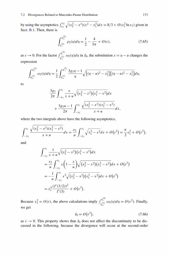
7.2 Divergences Related to Marcenko-Pastur Distribution 173
by using the asymptotics∫ x2x1
√(x2
2 − x2)(x2 − x21)dx = 8/3 +O(x2
1 lnx1) given inSect. B.1. Then, there is
∫ η(2)+
η(2)−
ρ2(η)dη = 1
2− 4
3π+O(ε), (7.65)
as ε → 0. For the factor∫ η(2)−η(1)+
ω2(η)dη in I0, the substitution x = η− u changes the
expression
∫ η(2)−
η(1)+
ω2(η)dη = 1
2
∫ η(2)−
η(1)+
3g3η− 1
η
√[(η− u)2 − x2
2
][(η− u)2 − x2
1
]dη,
to
3g3
2π
∫ x1
−x1
x
x + u
√(x2
2 − x2)(x2
1 − x2)dx
+ 3g3u− 1
2π
∫ x1
−x1
√(x2
2 − x2)(x21 − x2)
x + udx,
where the two integrals above have the following asymptotics,
∫ x1
−x1
√(x2
2 − x2)(x21 − x2)
x + udx = x2
u
∫ x1
−x1
√x2
1 − x2dx +O(ε2)= π
2x2
1 +O(ε2),
and∫ x1
−x1
x
x + u
√(x2
2 − x2)(x2
1 − x2)dx
= x2
u
∫ x1
−x1
x
(
1 − x
u
)√(x2
2 − x2)(x2
1 − x2)dx +O
(ε3)
= − 1
u
∫ x1
−x1
x2√(
x22 − x2
)(x2
1 − x2)dx +O
(ε3)
= x41(Γ (3/2))2
Γ (3)+O
(ε3).
Because x21 = O(ε), the above calculations imply
∫ η(2)−η(1)+
ω2(η)dη = O(ε2). Finally,
we get
I0 =O(ε2), (7.66)
as ε → 0. This property shows that I0 does not affect the discontinuity to be dis-cussed in the following, because the divergence will occur at the second-order
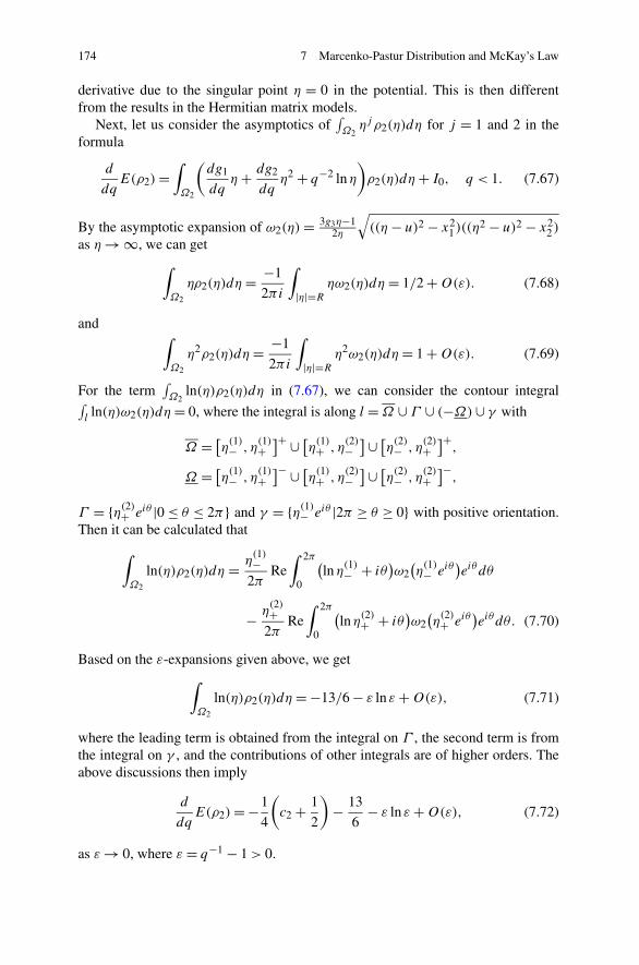
174 7 Marcenko-Pastur Distribution and McKay’s Law
derivative due to the singular point η = 0 in the potential. This is then differentfrom the results in the Hermitian matrix models.
Next, let us consider the asymptotics of∫Ω2
ηjρ2(η)dη for j = 1 and 2 in theformula
d
dqE(ρ2)=
∫
Ω2
(dg1
dqη+ dg2
dqη2 + q−2 lnη
)
ρ2(η)dη+ I0, q < 1. (7.67)
By the asymptotic expansion of ω2(η)= 3g3η−12η
√((η− u)2 − x2
1)((η2 − u)2 − x2
2)
as η → ∞, we can get∫
Ω2
ηρ2(η)dη = −1
2πi
∫
|η|=Rηω2(η)dη = 1/2 +O(ε). (7.68)
and∫
Ω2
η2ρ2(η)dη = −1
2πi
∫
|η|=Rη2ω2(η)dη = 1 +O(ε). (7.69)
For the term∫Ω2
ln(η)ρ2(η)dη in (7.67), we can consider the contour integral∫lln(η)ω2(η)dη = 0, where the integral is along l =Ω ∪ Γ ∪ (−Ω)∪ γ with
Ω = [η(1)− , η(1)+]+ ∪ [η(1)+ , η
(2)−]∪ [η(2)− , η
(2)+]+,
Ω = [η(1)− , η(1)+]− ∪ [η(1)+ , η
(2)−]∪ [η(2)− , η
(2)+]−,
Γ = {η(2)+ eiθ |0 ≤ θ ≤ 2π} and γ = {η(1)− eiθ |2π ≥ θ ≥ 0} with positive orientation.Then it can be calculated that
∫
Ω2
ln(η)ρ2(η)dη = η(1)−
2πRe∫ 2π
0
(lnη(1)− + iθ
)ω2(η(1)− eiθ
)eiθdθ
− η(2)+
2πRe∫ 2π
0
(lnη(2)+ + iθ
)ω2(η(2)+ eiθ
)eiθdθ. (7.70)
Based on the ε-expansions given above, we get∫
Ω2
ln(η)ρ2(η)dη = −13/6 − ε ln ε+O(ε), (7.71)
where the leading term is obtained from the integral on Γ , the second term is fromthe integral on γ , and the contributions of other integrals are of higher orders. Theabove discussions then imply
d
dqE(ρ2)= −1
4
(
c2 + 1
2
)
− 13
6− ε ln ε+O(ε), (7.72)
as ε → 0, where ε = q−1 − 1 > 0.

7.2 Divergences Related to Marcenko-Pastur Distribution 175
For ρ1, there are similar results, but the discussions are relatively easier. We firsthave
d
dqE(ρ1)=
∫
Ω1
(dg1
dqη+ dg2
dqη2 + q−2 lnη
)
ρ1(η)dη, q < 1. (7.73)
By the parameter relations (7.23) and (7.24), there are the following expansions,
q−1 = 1 + ε, ε > 0, b2 = 1 + 1
2ε− c1
12ε2 + · · · , (7.74)
g1 = 5 + c1ε+ · · · , g2 = −3
2− c1
6ε+ · · · , (7.75)
η− = a − 2b= 1
16ε2 + · · · , η+ = a + 2b = 4 + 3
2ε+ · · · , (7.76)
as ε → 0, with a constant c1. Then, we have∫Ω1
ηρ1(η)dη = 1/2 + O(ε) and∫Ω1
η2ρ1(η)dη = 1 + O(ε) similar to (7.68) and (7.69). And similar to (7.70), itcan be calculated that
∫Ω1
ln(η)ρ1(η)dη is equal to
η−2π
Re∫ 2π
0(lnη−+iθ)ω1
(η−eiθ
)eiθdθ− η+
2πRe∫ 2π
0(lnη++iθ)ω1
(η+eiθ
)eiθ dθ,
(7.77)which gives
∫
Ω1
ln(η)ρ1(η)dη = −13/6 − 2ε ln ε+O(ε). (7.78)
It should be noted that the coefficient of ε ln ε is changed to −2 if comparing withthe coefficient −1 in (7.71). So we have the following ε-expansion,
d
dqE(ρ1)= −c1
3− 13
6− 2ε ln ε+O(ε), (7.79)
as ε → 0, where ε = q−1 − 1 > 0.By comparing (7.72) with (7.79), it can be seen that if 4c1 − 3c2 = 3/2, then the
first-order derivative dE/dq is discontinuous. If c1 = c2 = 3/2, then 4c1 − 3c2 =3/2, and we have
d
dqE(ρ)=
{− 83 − 2|q − 1| ln |q − 1| +O(|q − 1|), ρ = ρ1,0 < q < 1,
− 83 − |q − 1| ln |q − 1| +O(|q − 1|), ρ = ρ2,0 < q < 1,
(7.80)
as q → 1. Finally we get the following second-order logarithmic divergence,
d2
dq2E =O
(ln |q − 1|), (7.81)

176 7 Marcenko-Pastur Distribution and McKay’s Law
as q → 1 − 0. It is interesting to note that in the case c1 = c2 = 3/2, for both ρ1and ρ2 phases the parameters g1, g2 and q stay on the same side of the critical pointwith the expansions
g1 = 5 + 3
2ε > 5, g2 = −3
2− 1
4ε <−3
2, q < 1. (7.82)
This property further indicates that the one-side transition would be specific forthe models reduced from the Laguerre polynomials or the generalizations since thepolynomials are defined on one side of the 0 point. The discontinuities of first orsecond order discussed above are to extend the Marcenko-Pastur distribution casefor studying a wider class of random behavioral problems. One can investigate morecomplicated models, but the divergences would always occur at the second-orderderivatives because of the singular point 0.
7.3 Jacobi Polynomials and Logarithmic Divergences
The Jacobi polynomials P (α,β)n (x) are defined on the interval [−1,1], and orthogo-
nal with the weight w(x)= (1 − x)α(1 + x)β ,
∫ 1
−1P (α,β)n (x)P
(α,β)
n′ (x)w(x)dx
= 2α+β+1
2n+ α + β + 1
Γ (n+ α + 1)Γ (n+ β + 1)
Γ (n+ +1)Γ (n+ α + β + 1)δnn′ , (7.83)
where α >−1, β >−1. Specially
P(α,β)
0 (x)= 1, P(α,β)
1 (x)= 1
2(α + β + 2)x + 1
2(α − β).
The Jacobi polynomials satisfy the following recursion formula and the differentialequation [35]:
2n(n+ α + β)(2n+ α + β − 2)P (α,β)n (x)
= (2n+ α + β − 1)[(2n+ α + β)(2n+ α + β − 2)x + α2 − β2]P (α,β)
n−1 (x)
− 2(n+ α − 1)(n+ β − 1)(2n+ α + β)P(α,β)
n−2 (x), n= 2,3, . . . , (7.84)
and
(2n+ α + β)(1 − x2) d
dxP (α,β)n (x)
= −n[(2n+ α + β)x + β − α]P (α,β)n (x)+ 2(n+ α)(n+ β)P
(α,β)
n−1 (x). (7.85)

7.3 Jacobi Polynomials and Logarithmic Divergences 177
Now, choose Φn(x) = w(x)1/2(P(α,β)n (x),P
(α,β)
n−1 (x))T . It can be verified thatΦn(x) satisfies the following equation [35]
∂
∂xΦn =An(x)Φn, (7.86)
where
An(x)= 1
1 − x2
(− α2−β2
2(2n+α+β) − (n+ α+β2 )x
2(n+α)(n+β)2n+α+β
− 2n(n+α+β)2n+α+β
α2−β2
2(2n+α+β) + (n+ α+β2 )x
)
.
(7.87)As a remark, the coefficients in the matrix An here do not have square roots for theparameters, that are different from the coefficients in the differential equations forthe Jacobi polynomials given in other literatures. Let p = α/n and q = β/n. Theabove formula implies
√detAn(x)
= n
1 − x2
√4(1 + p)(1 + q)(1 + p+ q)
(2 + p+ q)2−(
p2 − q2
2(2 + p+ q)+(
1 + p+ q
2
)
x
)2.
Specially, if p = q , there is the following result,
1
nπ
√detAn(x)dx = 1
π(1 − x2)
√1 + 2q − (q + 1)2x2dx. (7.88)
If we make change of the variable and parameter, x = η/c and q = c/2 − 1, thenthere is
1
π(1 − x2)
√1 + 2q − (q + 1)2x2dx = c
2π(c2 − η2)
√4(c− 1)− η2dη. (7.89)
The density function on the right hand side above is the McKay’s law [24]. Ifp = −q with −1 < q < 1, then
1
nπ
√detAn(x)dx = 1
π(1 − x2)
√1 − q2 − x2dx. (7.90)
It will discussed later that this density model does not have transition, which is thendifferent from the McKay’s law. A general eigenvalue density based on the Jacobipolynomials is discussed in the following.
When 1 + p > 0, 1 + q > 0, and 1 + p+ q > 0, denote
ω(η)= 1
1 − η2
√(p2 − q2
2(2 + p+ q)+(
1 + p+ q
2
)
η
)2− 4(1 + p)(1 + q)(1 + p+ q)
(2 + p+ q)2,
(7.91)

178 7 Marcenko-Pastur Distribution and McKay’s Law
which can be written as
ω(η)= 2 + p+ q
2(1 − η2)
√(η− η−)(η− η+), (7.92)
where
η− = q2 − p2 − 4√(1 + p)(1 + q)(1 + p+ q)
(2 + p+ q)2, (7.93)
η+ = q2 − p2 + 4√(1 + p)(1 + q)(1 + p+ q)
(2 + p+ q)2. (7.94)
We first have the following lemma by direct calculations, which will be appliedwhen computing the residue at η = −1 or η = 1.
Lemma 7.1
1
4
[p2 −q2 −(2+p+q)2
]2 −4(1+p)(1+q)(1+p+q)= q2(2+p+q)2. (7.95)
Lemma 7.2 For 1 + p > 0, 1 + q > 0, and 1 + p+ q > 0, there is
−1 ≤ η− ≤ η+ ≤ 1, (7.96)
where η− = −1 if q = 0, and η+ = 1 if p = 0.
Proof To prove −1 ≤ η−, consider 0 ≤ 4q2(2 + p+ q)2. By (7.95), this inequalitybecomes
16(1 + p)(1 + q)(1 + p+ q)≤ (q2 − p2 + (2 + p+ q)2)2.
Since q2 − p2 + (2 + p+ q)2 = 2((p+ q)(2 + q)+ 2) > 2((p+ q + 1)− q) > 0,we get
4√(1 + p)(1 + q)(1 + p+ q)≤ q2 − p2 + (2 + p+ q)2,
which implies −1 ≤ η−, where equality holds only if q = 0.For η+ ≤ 1, consider 0 ≤ 4p2(2 + p+ q)2. By (7.95), it becomes
16(1 + p)(1 + q)(1 + p+ q)≤ (p2 − q2 + (2 + p+ q)2)2.
Since p2 − q2 + (2 + p+ q)2 = 2((p+ q)(2 + p)+ 2) > 2((p+ q + 1)− p) > 0,we get
4√(1 + p)(1 + q)(1 + p+ q)≤ p2 − q2 + (2 + p+ q)2,
which gives η+ ≤ 1, where equality holds only if p = 0. �
The above lemme shows that η = 1 and η = −1 are in the domain C�Ω whereΩ = [η−, η+], and they are the poles of the analytic function ω. Then the ω function

7.3 Jacobi Polynomials and Logarithmic Divergences 179
is analytic in C�({−1} ∪Ω ∪ {1}). With these basic properties ready, we can nowdiscuss the variational equation.
Corresponding to the weight function w(x)= (1 − x)α(1 + x)β , we choose thepotential
W(η)= p ln(1 − η)+ q ln(1 + η), (7.97)
for the Jacobi model, and then W ′(η) = p/(η − 1) + q/(η + 1). In the Hermitianmodels, the ω function is usually asymptotic to W ′(η)/2 as η → ∞ as we have dis-cussed before. In the Laguerre models, W ′(η)/2 partially appears in the asymptoticsof the ω function. For the Jacobi models, there is no W ′(η)/2 in the asymptotics ofthe ω function. The following result shows that W ′(η)/2 will come out from theresidues of the ω function at the poles ±1.
Lemma 7.3 For the ω(η) defined by (7.91), there are
ω(η)= −(
1 + p+ q
2
)1
η+O
(1
η2
)
, (7.98)
as η → ∞, and
resη=1
ω(η)= −p
2, res
η=−1ω(η)= −q
2. (7.99)
Proof The asymptotics (7.98) directly follows from the definition (7.91) of the ω.For the residue at η = 1, we first note that (1 − η2)ω(η)|η=1 =√p2 = p by using(7.95) with a interchange between p and q , where
√p2 = p according to the branch
of the analytic function ω(η). Then,
resη=1
ω(η)= limη→1
(η− 1)ω(η)= − (1 − η2)ω(η)
1 + η
∣∣∣∣η=1
= −p
2.
At η = −1, there are (1 − η2)ω(η)|η=−1 = e2πi/2q = −q , and
resη=−1
ω(η)= limη→−1
(η+ 1)ω(η)= (1 − η2)ω(η)
1 − η
∣∣∣∣η=−1
= −q
2.
Then the lemma is proved. �
Now, define
ρ(η)= 1
πiω(η)
∣∣∣∣Ω+
, (7.100)
for η ∈Ω .
Theorem 7.3 The ρ(η) defined by (7.100) satisfies the normalization∫
Ω
ρ(η)dη= 1, (7.101)

180 7 Marcenko-Pastur Distribution and McKay’s Law
Fig. 7.3 Contours forMcKay’s law
and the variational equation
(P)∫
Ω
ρ(η)
η− λdη= 1
2W ′(λ), (7.102)
where λ is an inner point of Ω .
Proof Let Γ be a large counterclockwise circle of radius R with center 0, Γ ε−1 and
Γ ε1 be the counterclockwise circles of radius ε with centers −1 and 1 respectively,
and Ω∗ be the union of the closed counterclockwise contours around the upper andlower edges of Ω , or Ω∗ = Ω− ∪ (−Ω+). See Fig. 7.3. Then Cauchy theoremimplies
{∫
Ω∗+∫
Γ ε−1
+∫
Γ ε1
−∫
Γ
}
ω(η)dη= 0,
or
−∫
Ω
ρ(η)dη− p+ q
2+(
1 + p+ q
2
)
= 0,
and then (7.101) is proved.To prove (7.102), we need to change Ω∗ at the inner point λ ∈ Ω . The Ω−
and Ω+ around λ can be changed to the semicircles of ε radius. If we still use theprevious notations, then
{∫
Ω∗+∫
Γ ε−1
+∫
Γ ε1
−∫
Γ
}ω(η)
η− λdη = 0,
which implies
−2(P)∫
Ω
ρ(η)
η− λdη+ p
λ− 1+ q
λ+ 1= 0,
where the integral∫Γ
disappears, and∫Γ ε−1
and∫Γ ε
1give the last two terms above.
Here we have used∫ 0−π ω(λ+ εeiθ )dθ + ∫ π0 ω(λ+ εeiθ )dθ → 0 as ε → 0 due to

7.3 Jacobi Polynomials and Logarithmic Divergences 181
the opposite signs of the ω in these two integrals, where the integral path of the firstintegral is below Ω and the second integral is above Ω . �
If we consider the following quantity
E =∫ η+
η−W(η)ρ(η)dη−
∫ η+
η−
∫ η+
η−ln |η− λ|ρ(η)ρ(λ)dηdλ, (7.103)
for small p and q by choosing p = c1ε and q = c2ε, then we have
dE
dε= c1
∫ η+
η−ln(1 − η)ρ(η)dη+ c2
∫ η+
η−ln(1 + η)ρ(η)dη. (7.104)
Then by (7.93) and (7.94) there are
η− = −1 + c22
2ε2 + · · · , η+ = 1 − c2
1
2ε2 + · · · . (7.105)
To compute∫ η+η− ln(1 − η)ρ(η)dη, consider
{∫
Γ
+∫
Ω++∫
γ
−∫
Ω−
}
ln(η)ω(η)dη = 0,
for the closed contour Γ ∪Ω+ ∪ γ ∪ (−Ω−) with positive orientation, where the“−” sign before Ω− stands for the opposite orientation, Ω+ and Ω− are the upperand lower edges of Ω , γ is the small circle |η−1| = 1−η+ (or η−1 = (η+ −1)eiθ
with 2π ≥ θ ≥ 0), and Γ is the circle |η− 1| = 1 −η− (or η− 1 = (η− − 1)eiθ with0 ≤ θ ≤ 2π ). By the ε-expansions (7.105), we have
∫ η+
η−ln(1 − η)ρ(η)dη
= 1
2πRe
( |c1|2ε
∫ 2π
0
(ln(1 + η+)+ iθ
)√1 − eiθdθ
)
− 1
2πRe
(∫ 2π
0
(ln(1 − η−)+ iθ
)√(eiθ − 1)eiθ
1 − eiθdθ
)
+O(ε), (7.106)
as ε → 0. By the formulas given in Appendix A, we can get∫ η+
η−ln(1 − η)ρ(η)dη = − ln 2 + |c1|ε ln ε+O(ε). (7.107)
Similarly, as ε → 0, there is∫ η+
η−ln(1 + η)ρ(η)dη = − ln 2 + |c2|ε ln ε+O(ε). (7.108)

182 7 Marcenko-Pastur Distribution and McKay’s Law
Therefore, we have
dE
dε= −(c1 + c2) ln 2 + (c1|c1| + c2|c2|
)ε ln ε+O(ε), (7.109)
as ε → 0, that gives a logarithmic divergence for the second-order derivative of Eif c1|c1| + c2|c2| = 0.
If p = −q for |q|< 1 corresponding to c1 + c2 = 0, then
dE
dq=∫ η0
−η0
ln1 + η
1 − ηρ(η)dη, (7.110)
where ρ(η)=√
1−q2−η2
π(1−η2), given by (7.90), and η0 =√1 − q2 < 1. It follows that
dE
dq= 2
∞∑
n=1
1
2n− 1
∫ η0
−η0
η2n−1
√η2
0 − η2
1 − η2dη = 0, (7.111)
because of the odd symmetry of the functions, and thenE is a constant in this specialcase.
If p or q is large, we can consider p = c/τ and q = c2/τ with τ → 0. If c2 = 0and c1 > 0, then η− = 1 +O(τ) and η+ = 1 +O(τ) as τ → 0, that imply
dE
dτ=O(ln τ), (7.112)
as τ → 0. There is similar result if c1 = 0 and c2 > 0. If c1 > c2 > 0, then η± →(c2 − c1)/(c1 + c2) as τ → 0. Then we have
dE
dτ=O(1), (7.113)
as τ → 0. The case c2 > c1 > 0 is similar. If c1 = c2 > 0, then η± →O(τ 1/2), and
dE
dτ=O
(τ 1/2), (7.114)
as τ → 0.This type mathematical problems have drawn lot attentions in recent years,
specially in the researches for the entanglement problems. Many literatures havebeen published in the field about the entanglement or entropy with variousmethods including correlation functions, quantum disorder, quantum phase tran-sition, density matrix and matrix Riemann-Hilbert problems. Interested read-ers can find the discussions, for example, in [1, 7, 10, 14, 20, 38]. As a re-mark, the function ω(η) discussed above satisfies the following properties: ω(η)is analytic for η ∈ C�({−1} ∪ Ω ∪ {1}) with the first-order poles η = ±1;ω(η)|Ω+ +ω(η)|Ω− = 0; ω(η)→ 0 as η → ∞. We know that the scalar Riemann-Hilbert problem: ω(η)|Ω+ +ω(η)|Ω− = 0; ω(η) → 0 as η → ∞ has the unique

7.4 Integral Transforms for the Density Functions 183
trivial solution ω(η) = 0. When two poles ±1 are added in the problem, the so-lution is not trivial. There would be more interesting properties for the modifiedproblems if more poles are added, that are left for further investigations.
7.4 Integral Transforms for the Density Functions
We have obtained the power-law and logarithmic divergences of the derivatives ofthe free energy functions based on the integrals of the density functions in the pre-vious discussions. The exponent in the power-law divergence at the critical point iscalled critical exponent that can be used to classify the diverse transition systems.The systems with the same critical exponent belong to the same universality classaccording to the renormalization group theory because they have the same scalingbehavior and share the same fundamental dynamics. We have seen that the power-law divergence depends on the potential and the expansions of the parameters atthe critical point, and the logarithmic divergence is a limit case of the power-lawdivergence [3]. We have also seen that the power-law divergence is not directly con-nected to the power formula of the eigenvalue density. In this section, we are goingto show that the power formula of the eigenvalue density can be applied to get thepower-law distribution by using the integral transforms.
Let us use the Laplace transform to show that the eigenvalue densities in thematrix models can be transformed to the power-law distributions that are importantin the complexity researches. Consider the Wigner semicircle
ρ(η)= 1
2b2π
√4b2 − (η− a)2, (7.115)
which satisfies∫ a+2ba−2b ρ(η)dη = 1. For the convenience in the discussions below, we
consider the case 2b− a > 0. Let
p(x)= c0
∫ a+2b
a−2be−x(η−a+2b)μρ(η)dη, 0 <μ<
3
2, (7.116)
with a constant c0 > 0. We want to show that p(x) is a power-law distribution func-tion for x ≥ 0.
First, p(x) is well defined for the parameters given above with the correspondingrestrictions. It is easy to see that p(0)= c0 > 0, p(x) > 0 for x > 0, and p′(x) < 0for x > 0. To show
∫∞0 p(x)dx = 1, consider
I (t)=∫ ∞
0
∫ a+2b
a−2be−x(tη−a+2b)μ
√4b2 − (η− a)2dηdx, (7.117)
for 0 ≤ t ≤ 1. Taking derivative with respect to t on both sides of the equation above,after simplification by using
∫∞0 xe−x(tη−a+2b)μdx = (tη− a + 2b)−2μ, we have
I ′(t)= −μ∫ a+2b
a−2bη
√4b2 − (η− a)2(tη− a + 2b)−μ−1dη. (7.118)

184 7 Marcenko-Pastur Distribution and McKay’s Law
It follows that by taking integral for t from 0 to 1,
I (1)− I (0)=∫ a+2b
a−2b
√4b2 − (η− a)2
[(η− a + 2b)−μ − (2b− a)−μ
]dη,
where t = 1 means t → 1 − 0 to avoid the singularity when η = a − 2b. SinceI (0)= 2b2π/(2b− a)μ, we then get
I (1)=∫ 2b
−2b
√4b2 − ζ 2
(ζ + 2b)μdζ, (7.119)
where ζ = η − a. The integral is convergent since the integrand is of O((ζ +2b)1/2−μ) as ζ → −2b with 1/2−μ>−1. Then, I (1)= (4b)2−μB(3/2,3/2−μ),where B(·, ·) is the Euler beta function. Therefore, we finally obtain
∫ ∞
0p(x)dx = c0
2b2πI (1)= c0
2b2π(4b)2−μB(3/2,3/2 −μ), (7.120)
which implies that if
c0 = (4b)μπ
8B(3/2,3/2 −μ), (7.121)
then∫∞
0 p(x)dx = 1 and p(x) is a distribution function.Next, let us show p(x) has a power-law asymptotics as x → ∞. Consider the
following integral∫ δ
0e−xζμζ ν−1dη, (7.122)
where δ > 0 is a fixed number. Let t = xημ. It follows that [26]
∫ δ
0e−xζμην−1dη= 1
μxνμ
∫ xδμ
0e−t t
νμ
−1dt = Γ (ν/μ)
μxν/μ+ o(x−ν/μ),
as x → ∞. The asymptotics of p(x) as x → ∞ is dominated by the behavior ofρ(η) at η = a− 2b as known in the Laplace asymptotics method [26]. Since ρ(η)=O((ζ )1/2) as ζ → 0, where ζ = η− a+ 2b, the asymptotic behavior of p(x) can be
obtained by (7.122) for ν = 3/2. Then we get p(x)=O(x− 3
2μ ) as x → ∞.Sometimes, the ν can be a different number. For example, for the critical density
ρc(η)= 1
2b2π
(4b2 − (η− a)2
)3/2, (7.123)
we have ν = 5/2, that will give a distribution with the power-law O(x− 5
2μ ) asx → ∞. As known in the random matrix theory, the eigenvalue density is obtainedfrom the correlation function in large-N asymptotics. When N = 1, the correlation

7.4 Integral Transforms for the Density Functions 185
function is the Gaussian distribution. If we consider the Laplace transform of theGaussian distribution
p0(x)=∫ ∞
0e−xη2
e−η2dη, (7.124)
it can by seen that
p0(x)= ex2/4∫ ∞
x/2e−t2dt =O
(x−1), (7.125)
as x → ∞. The above discussions can be also applied to other eigenvalue densities,such as the Marcenko-Pastur distribution, McKay’s law and Gross-Witten densities.
If we consider the Laplace transform for the Marcenko-Pastur distribution (7.12),
∫ ∞
0e−ξη Re
1
πiω0(η)dη =
∫ η+
η−e−ξηρ0(η)dη, (7.126)
then by the asymptotics∫ δ
0 e−ξηην−1dη = Γ (ν)
ξν+ o(ξ−ν) as ξ → ∞, we can get
a power-law ξ−3/2, since ρ0(η) = O((η − η−)1/2) as η → η−. If we consider thecritical case q = 1 with η− = 0 and η+ = 4,
ρc0(η)= 1
2π
√4 − η
η, (7.127)
then we get a power-law ξ−1/2 as ξ → ∞, since ρc0(η) = O(η−1/2) as η → 0.The corresponding “distribution” function is then not integrable, that indicates asingularity in the case q = 1, consistent with the transition phenomenon discussedbefore. More complicated integral transforms can be studied similarly.
The power-law distribution is an important research topic in the complexity sub-jects such as econophysics, for example, see [4, 18, 19, 22, 28, 29, 33]. The asso-ciated researches include random matrices and phase transitions, that can be found,for example, in [2, 9, 11, 17, 21, 27, 29, 34, 40–42]. Another related field is about theoverreactions and herding behaviors in the behavioral sciences that have also drawnlot attentions in recent years, and many literatures in these subjects have been pub-lished, for example, see [6, 13, 16, 31, 32, 36]. Since this book is organized based onthe integrable systems, we are not going to discuss the details of these researches.These references are listed here in order to remind the interested readers to pay at-tentions to the related new researches. In the following, we are going to show moreproperties about the density models and the power-laws.
To discuss the power-law by using the Fourier transform, let us review a basicproperty discussed in the method of stationary phase [26]. Consider the integral∫ δ
0 eiξηην−1dη, where δ > 0 is a fixed number and 0 < ν < 1. As shown in [26],
the integration around the contour {η|ε ≤ Reη ≤ R, Imη = 0} ∪ {η|0 ≤ argη ≤π/2, |η| =R} ∪ {η|ε ≤ Imη ≤R,Reη = 0} ∪ {η|0 ≤ arg ≤ π/2, |η| = ε} yields

186 7 Marcenko-Pastur Distribution and McKay’s Law
∫ ∞
0eiξηην−1dη = eνπi/2Γ (ν)
ξν. (7.128)
Then∫ δ
0eiξηην−1dη=
{∫ ∞
0−∫ ∞
δ
}
eiξηην−1dη= eνπi/2Γ (ν)
ξν+ o(ξ−ν),
as ξ → ∞. Applying this asymptotic expansion to the densities discussed above, wecan get the power-law ξ−3/2 or ξ−5/2 as ξ → ∞.
Now, if we consider the moments∫ η+η− ηjρ(η)dη discussed in the free energy
function, it can be seen that they are in fact the Mellin transform∫∞
0 ηξ−1ρ(η)dη
when ξ is an integer, where ρ has a finite support. We are going to show the follow-ing relations for the moment quantities,
∫ ∞
0
xj
nπRe√
detAn(x)dx =∫ ∞
0xj+αe−xKn(x, x)dx, (7.129)
for j = 0,1,2, where Kn(x, y) is the Fredholm kernel for the Laguerre polynomials[35],
Kn(x, y)= 1
n
n−1∑
k=0
1
hkL(α)k (x)L
(α)k (y)= 1
hn−1
L(α)n (x)L
(α)n−1(y)−L
(α)n (y)L
(α)n−1(x)
x − y,
(7.130)with hk = Γ (α+ 1)( k+α
k). For j = 0, the right hand side of (7.129) is equal to 1 by
the definition. By Theorem 7.1, the left hand side is also equal to 1 when j = 0.To prove the relation for j = 1,2, we first note that
Kn(x, x)= 1
hn−1
(
L(α)n (x)d
dxL(α)n−1(x)−L
(α)n−1(x)
d
dxL(α)n (x)
)
.
By the recursion formula (7.2) and the differential equation (7.3), we can get
x
(
L(α)n (x)d
dxL(α)n−1(x)−L
(α)n−1(x)
d
dxL(α)n (x)
)
= −L(α)n (x)(L(α)n−1(x)+ (n− 1 + α)L
(α)n−2(x)
)+ (n+ α)L(α)n−1(x)L
(α)n−1(x),
and
x2(
L(α)n (x)d
dxL(α)n−1(x)−L
(α)n−1(x)
d
dxL(α)n (x)
)
= [(n+ 1)L(α)n+1(x)− (2n+ 1 + α + n(n+ α))L(α)n (x)
]L(α)n−1(x)
+ [(n+ α)(2n+ α)L(α)n−1(x)− (n+ α)(n− 1 + α)L
(α)n−2(x)
]L(α)n−1(x)
− (n− 1 + α)xL(α)n (x)L(α)n−2(x).

References 187
Then∫ ∞
0x1+αe−xKn(x, x)dx = n+ α, (7.131)
and∫ ∞
0x2+αe−xKn(x, x)dx = (n+ α)(2n+ α). (7.132)
For the left hand side of (7.129), we have the asymptotics
√−detAn(x) = 1
2−(
n+ α
2
)
x−1 − n(n+ α)x−2 − n(n+ α)(2n+ α)x−3
+O(x−4),
as x → ∞. Consequently, there are the following results
∫ ∞
0
x
nπRe√
detAn(x)dx = n+ α, (7.133)
and∫ ∞
0
x2
nπRe√
detAn(x)dx = (n+ α)(2n+ α). (7.134)
Therefore we have proved (7.129) for j = 1 and 2. It is left to interested readers toverify whether (7.129) is true when j > 2.
The integral transforms of the density models have been discussed to give differ-ent power-laws connected to the different phases in the density transition models.In some sense, the integral transforms change the problem to be viewed from adifferent point so that the mathematical properties in the different aspects can becompared and referred, for example, when the uncertainty is involved in the con-sideration. We have seen that the integrable systems can be applied to solve manytransition problems. And the importance of the integrable systems is not limitedto these problems. One can associate other theories with the integrable systems todevelop further methods and solve more application problems.
References
1. Ali, M., Rau, A.R.P., Alber, G.: Quantum discord for two-qubit X-states. Phys. Rev. A 81,042105 (2010), see also Erratum, Phys. Rev. A 82, 069902(E) (2010)
2. Andriani, P., McKelvey, B.: Beyond Gaussian averages: redirecting organization science to-ward extreme events and power laws. J. Int. Bus. Stud. 38, 1212–1230 (2007)
3. Binney, J.: The Theory of Critical Phenomena: an Introduction to the Renormalization Group.Oxford University Press, London (1992)
4. Biroli, G., Bouchaud, J.P., Potters, M.: On the top eigenvalue of heavy-tailed random matrices.Europhys. Lett. 78, 10001 (2007)

188 7 Marcenko-Pastur Distribution and McKay’s Law
5. Bouchaud, J.-P., Potters, M.: Theory of Financial Risks. Cambridge University Press, Cam-bridge (2001)
6. Caginalp, G., Porter, D., Smith, V.: Momentum and overreaction in experimental asset mar-kets. Int. J. Ind. Organ. 18, 187–204 (2000)
7. Dillenschneider, R.: Quantum discord and quantum phase transition in spin chains. Phys. Rev.B 78, 224413 (2008)
8. Emerson, J., Weinstein, Y.S., Saraceno, M., Lloyd, S., Cory, D.G.: Pseudo-random unitaryoperators for quantum information processing. Science 302, 2098 (2003)
9. Frahm, G., Jaekel, U.: Random matrix theory and robust covariance matrix estimation forfinancial data. arXiv:physics/0503007 (2005)
10. Gu, S.J., Tian, G.S., Lin, H.Q.: Local entanglement and quantum phase transition in spinmodels. New J. Phys. 8, 61 (2006)
11. Harré, M., Bossomaier, T.: Phase-transition-like behaviour of information measures in finan-cial markets. Europhys. Lett. 89, 18009 (2009)
12. Harrow, A.W., Low, R.A.: Random quantum circuits are approximate 2-designs. Commun.Math. Phys. 291, 257–302 (2009)
13. Hong, H., Stein, J.: A unified theory of underreaction, momentum, and overreaction in assetmarkets. J. Finance 54, 2143–2184 (1999)
14. Its, A.R., Jin, B.Q., Korepin, V.E.: Entanglement in XY spin chain. J. Phys. A, Math. Gen. 38,2975 (2005)
15. Johansen, A., Sornette, D., Ledoit, O.: Crashes as critical points. Int. J. Theor. Appl. Finance3, 219–255 (2000)
16. Kahneman, D., Tversky, A.: Prospect theory: an analysis of decision under risk. EconometricaXLVII, 263–291 (1979)
17. Kasprzak, A., Kutner, R., Perelló, J., Masoliver, J.: Higher-order phase transitions on financialmarkets. Eur. Phys. J. B 76, 513–527 (2010)
18. Kaulakys, B., Meskauskas, T.: Modeling 1/f noise. Phys. Rev. E 58, 7013–7019 (1998)19. Kaulakys, B., Ruseckas, J., Gontis, V., Alaburda, M.: Nonlinear stochastic models of 1/f noise
and power-law distributions. Physica A 365, 217–221 (2006)20. Kitaev, A., Preskill, J.: Topological entanglement entropy. Phys. Rev. Lett. 96, 110404 (2006)21. Majumdar, S.N., Vergassola, M.: Large deviations of the maximum eigenvalue for Wishart
and Gaussian random matrices. Phys. Rev. Lett. 102, 060601 (2009)22. Mantegna, R.N., Stanley, H.E.: An Introduction to Econophysics: Correlation and Complexity
in Finance. Cambridge University Press, Cambridge (2000)23. Marcenko, V.A., Pastur, L.A.: Distribution of eigenvalues for some sets of random matrices.
Mat. Sb. 72(114)(4), 507–536 (1967)24. McKay, B.D.: The expected eigenvalue distribution of a large regular graph. Linear Algebra
Appl. 40, 203–216 (1981)25. McLeod, J.B., Wang, C.B.: Eigenvalue density in Hermitian matrix models by the Lax pair
method. J. Phys. A, Math. Theor. 42, 205205 (2009)26. Olver, F.W.J.: Asymptotics and Special Functions. Academic Press, New York (1974)27. Ormerod, P., Mounfield, C.: Random matrix theory and the failure of macroeconomic fore-
casts. Physica A 280, 497–504 (2000)28. Plerou, V., Gopikrishnan, P., Rosenow, B., Amaral, L.A.N., Guhr, T., Stanley, H.E.: Random
matrix approach to cross correlations in financial data. Phys. Rev. E 65, 066126 (2002)29. Plerou, V., Gopikrishnan, P., Stanley, H.E.: Two-phase behaviour of financial market. Nature
421, 130 (2003)30. Sengupta, A.M., Mitra, P.P.: Distributions of singular values for some random matrices. Phys.
Rev. E 60, 3389–3392 (1991)31. Shefrin, H.: Beyond Greed and Fear: Understanding Behavioral Finance and the Psychology
of Investing. Oxford University Press, London (2002)32. Shefrin, H., Statman, M.: Behavioral portfolio theory. J. Financ. Quant. Anal. 35, 127–151
(2000)
References 189
33. Simon, S.H., Moustakas, A.L.: Eigenvalue density of correlated complex random Wishartmatrices. Phys. Rev. E 69, 065101(R) (2004)
34. Sornette, D.: Critical Phenomena in Natural Sciences: Chaos, Fractals, Self Organization andDisorder: Concepts and Tools, 2nd edn. Springer, Berlin (2004)
35. Szegö, G.: Orthogonal Polynomials, 4th edn. American Mathematical Society ColloquiumPublications, vol. 23. AMS, New York (1975)
36. Thaler, R.H.: Towards a positive theory of consumer choice. J. Econ. Behav. Organ. 1, 39–60(1980)
37. Van Assche, W.: Discrete Painlevé equations for recurrence coefficients of orthogonal poly-nomials. In: Proceedings of the International Conference on Difference Equations, SpecialFunctions and Orthogonal Polynomials, pp. 687–725. World Scientific, Hackensack (2007)
38. Vidal, G., Latorre, J.I., Rico, E., Kitaev, A.: Entanglement in quantum critical phenomena.Phys. Rev. Lett. 90, 227902 (2003)
39. Vivo, P., Majumdar, S.N., Bohigas, O.: Large deviations of the maximum eigenvalue inWishart random matrices. J. Phys. A, Math. Theor. 40, 4317 (2007)
40. Wishart, J.: The generalized product moment distribution in samples from a normal multivari-ate population. Biometrika 20A, 32–52 (1928)
41. Yalamova, R.: Correlations in Financial Time Series During Extreme Events—Spectral Clus-tering and Partition Decoupling Method. Proceedings of the World Congress on Engineering2009, vol. II. WCE, London (2009)
42. Yalamova, R., McKelvey, B.: Explaining what leads up to stock market crashes: a phase tran-sition model and scalability dynamics. In: 2nd International Financial Research Forum Paris(2009)

Appendix ASome Integral Formulas
In Sect. 3.1, it is discussed that the free energy in the Hermitian matrix model can becalculated based on the moments
∫ η+η− ηkρ(η)dη and
∫ η+η− ln |η − a|ρ(η)dη. These
integrals can be expressed in terms of
Rl,k = i
π
∫ π
−π(a + 2b cos θ)ke−ilθ sin θdθ, (A.1)
and
Θl = Rei
π
∫ π
0θeiθ
[(eiθ +
√e2iθ − 1
)l − (eiθ −√e2iθ − 1
)l]dθ, (A.2)
where l is integer. The term (a + 2b cos θ)k in (A.1) is from the potential, and theterm e−ilθ is from the eigenvalue density. It is seen that the integrals in (A.1) are theFourier transforms, that reflect an element of correlation function since the corre-lation functions are usually studied by using the Fourier transforms and are relatedto the partition function which is reduced to the free energy function now. The in-tegrals in (A.2) are modified transforms indicating that the discussion is not limitedto the traditional Fourier transform.
It has been given in Sect. 3.1 that we need to use
Yl = 1
2
4∑
k=0
gkRl,k +Θl, (A.3)
for l = 1,2 and 3 to calculate the free energy when m = 2. If we denote Y =(Y1, Y2, Y3)
T , g = (g0, g1, g2, g3, g4)T , Θ = (Θ1,Θ2,Θ3)
T , and R = (Rl,k)3×5,the above formula becomes
Y = 1
2Rg +Θ. (A.4)
C.B. Wang, Application of Integrable Systems to Phase Transitions,DOI 10.1007/978-3-642-38565-0, © Springer-Verlag Berlin Heidelberg 2013
191

192 A Some Integral Formulas
The Rl,k’s have the following results,
R1,0 = 1, R1,1 = a, R1,2 = a2 + b2, R1,3 = a(a2 + 3b2),
R1,4 = a4 + 2b4 + 6a2b2, R2,0 = 0, R2,1 = b, R2,2 = 2ab,
R2,3 = b(3a2 + 2b2), R2,4 = 4ab
(a2 + 2b2), R3,0 = 0, R3,1 = 0,
R3,2 = b2, R3,3 = 3ab2, R3,4 = 3b2(2a2 + b2).
Based on the discussions in Sect. 3.1, we have
Θ1 = − 2
πRe∫ π
0θeiθ
(1 − e2iθ ) 1
2 dθ = 4
πd0,
Θ2 = − 4
πRe∫ π
0θe2iθ (1 − e2iθ ) 1
2 dθ = 0,
Θ3 = 8
πRe∫ π
0θeiθ
(1 − e2iθ ) 3
2 dθ − 6
πRe∫ π
0θeiθ
(1 − e2iθ ) 1
2 dθ
= 4
π(3d0 − 4d1),
where
lk =∫ 1
0
(1 − x2)k+ 1
2 dx, (A.5)
dk =∫ 1
0
∫ 1
0
(1 − x2y2)k+ 1
2 dxdy (A.6)
for k = 0,1, . . . . Then, we finally get Θ1 = 12 + ln 2,Θ2 = 0,Θ3 = − 3
4 , based onthe following values
l0 = π
4, l1 = 3π
16, l2 = 15π
96, (A.7)
d0 = π
8+ π
4ln 2, d1 = 9π
64+ 3π
16ln 2, d2 = 55π
384+ 15π
96ln 2. (A.8)
In addition, we have the following basic formulas,
∫ 2π
0θ√
1 − eiθ dθ = 2π2 + 4π
i(ln 2 − 1), (A.9)
∫ 2π
0θ√
1 − e2iθ dθ = 2π2 + 2π
i(ln 2 − 1), (A.10)
∫ 2π
0θeiθ
√1 − e2iθ dθ = π2
2i, (A.11)

A Some Integral Formulas 193
∫ 2π
0θe2iθ
√1 − e2iθ dθ = 2π
3i, (A.12)
∫ π
0θeiθ
(1 − e2iθ )−1/2
dθ = −π ln 2 + π2
2i. (A.13)
To show (A.13), we need d−1 = ∫ 10
∫ 10 (1 − x2y2)−1/2dxdy = π
2 ln 2. These formu-las and the similar formulas given in Sect. 3.1 are often needed in the calculations.

Appendix BProperties of the Elliptic Integrals
B.1 Asymptotics of the Elliptic Integrals
Now, we want to show that for 0 < x1 < x2, there is
∫ x2
x1
√(x2
2 − x2)(x2 − x2
1
)dx = x3
2
3− x2
1x2
2
[
ln
(4x2
x1
)
− 1
2
]
+O(x4
1 lnx1), (B.1)
as x1 → 0.The expansion for the elliptic integral is achieved by using the contour integration
such that the different orders of the small terms can be separated. For this problem,
we consider the function f (z)= ln z√(x2
2 − z2)(z2 − x21), where the branch cut for
ln z is the upper edge of the negative real axis. The function f (z) is analytic in thedomain enclosed by the contour γ , where
γ = [x1, x2]+ ∪ {x2eiθ |0 ≤ θ ≤ π
}∪ [−x2,−x1]+ ∪ {x1eiθ |π ≥ θ ≥ 0
},
that implies∫γf (z)dz= 0, or
∫ −x1
−x2
f (z)dz+ x1
∫ 0
π
f(x1e
iθ)ieiθ dθ +
∫ x2
x1
f (z)dz+ x2
∫ π
0f(x2e
iθ)ieiθ dθ
= 0.
The contour integrals can separate the different orders of the small terms so that theanalysis become easier. By taking the imaginary parts on both sides and noting that√(x2
2 − z2)(z2 − x21) is negative on [−x2,−x1] as discussed in Sect. 3.3, we obtain
∫ x2
x1
√(x2
2 − x2)(x2 − x2
1
)dx = x2
2
πRe I2 − x2
1
πRe I1, (B.2)
C.B. Wang, Application of Integrable Systems to Phase Transitions,DOI 10.1007/978-3-642-38565-0, © Springer-Verlag Berlin Heidelberg 2013
195

196 B Properties of the Elliptic Integrals
where
I1 =∫ π
0(lnx1 + iθ)
√(x2
2 − x21e
2iθ)(e2iθ − 1
)eiθ dθ,
I2 =∫ π
0(lnx2 + iθ)
√(1 − e2iθ
)(x2
2e2iθ − x2
1
)eiθ dθ.
By using the integral formulas given in Appendix A, we can get
1
πRe I1 = −x2
2
[
ln(x1/2)− 1
2
]
+O(x2
1 lnx1),
1
πRe I2 = x2
2− x2
1
2x2
(ln(2x2)− 1
)+O(x4
1
),
and then the asymptotic expansion above can be obtained.The asymptotics above is applied to study the third-order transition in Sect. 3.4
for the Hermitian matrix model. The following asymptotics is applied to study thediscontinuity in the Laguerre model for the generalized Marcenko-Pastur distribu-tion discussed in Sect. 7.2.
For 0 < x1 < x2 < u, there is∫ x2
x1
x
x + u
√(x2
2 − x2)(x2 − x2
1
)dx = u
4
(2u2 − x2
2
)π + x3
2
3− x2u
2
+ iu2√u2 − x2
2 ln
(u+ x2 − i
√u2 − x2
2
u+ x2 + i
√u2 − x2
2
·x2 + i
√u2 − x2
2
x2 − i
√u2 − x2
2
)
+O(x2
1
), (B.3)
as x1 → 0. To show this asymptotics, consider f (z)= zz+u ln z
√(x2
2 − z2)(z2 − x21),
where the branch cut for ln z is the lower edge of the positive real axis. Then thereis∫γ1∪γ2
f (z)dz= 0, where
γ1 = [x1, x2]+ ∪ {x2eiθ |0 ≤ θ ≤ π
}∪ [−x2,−x1]+ ∪ {x1eiθ |π ≥ θ ≥ 0
},
and
γ2 = (−[−x2,−x1]−)∪{x2e
iθ |π ≤ θ ≤ 2π}∪(−[x1, x2]−
)∪{x1eiθ |2π ≥ θ ≥ π
}.
By taking the imaginary parts on both sides of∫γ1∪γ2
f (z)dz= 0, we can get
∫ x2
x1
x
x + u
√(x2
2 − x2)(x2 − x2
1
)dx = x3
2
2πRe I2 − x3
1
2πRe I1, (B.4)
where
I1 =∫ 2π
0
lnx1 + iθ
u+ x1eiθ
√(x2
2 − x21e
2iθ)(e2iθ − 1
)e2iθ dθ,

B.2 Elliptic Integrals Associated with Legendre’s Relation 197
I2 =∫ π
0
lnx2 + iθ
u+ x2eiθ
√(1 − e2iθ
)(x2
2e2iθ − x2
1
)e2iθ dθ.
Based on the integral formulas given in Appendix A and
∫ 2π
0θ
√1 − e2iθ
1 + r−1eiθdθ
= 2π
i
(
ln 2 − π
2r − i
√r2 − 1 ln
r + 1 − i√r2 − 1
r + 1 + i√r2 − 1
· 1 + i√r2 − 1
1 − i√r2 − 1
)
, (B.5)
where r = u/x2 and Re I1 =O(lnx1) as x1 → 0, we can get (B.3).
B.2 Elliptic Integrals Associated with Legendre’s Relation
Consider
ρ(x)= 1
2π
(3g3 + 4g4(x + 3u)
)√(x2
2 − x2)(x2 − x2
1
), (B.6)
for x ∈Ωρ = [−x2,−x1] ∪ [x1, x2], and
ω(x)= 1
2
(3g3 + 4g4(x + 3u)
)√(x2
1 − x2)(x2
2 − x2), (B.7)
for x ∈Ωω = [−x1, x1], where 0 ≤ x1 < x2 defined by
x21 = 1
4(a1 − a2)
2 + (b1 − b2)2, x2
2 = 1
4(a1 − a2)
2 + (b1 + b2)2, (B.8)
u= (a1 + a2)/2, and the parameters satisfy the conditions
3g3 + 4g4(x1 + 3u)≥ 0, 3g3 + 4g4(−x1 + 3u)≤ 0, (B.9)
where 4g4b21b
22 = 1 as discussed in Chap. 3, such that ρ(x) is non-negative on Ωρ .
We want to discuss the minimum value of the quantity
l0 = c1
∫ x1
−x1
ω(x)dx + c2
∫ x2
x1
ρ(x)dx, (B.10)
for the given constants c1 and c2 when the parameters change in the allowed re-gion(s). The above formula can be changed to
l0 − c2
2= 3
2(g3 + 4g4u)
(
c1I1 + c2
πI2
)
, (B.11)

198 B Properties of the Elliptic Integrals
where
I1 =∫ x1
−x1
√(x2
1 − x2)(x2
2 − x2)dx ≥ 0,
I2 =∫ x2
x1
√(x2
2 − x2)(x2 − x2
1
)dx ≥ 0,
(B.12)
since [−x1, x1] is between the two cuts [−x2,−x1] and [x1, x2]. Here, we have used
2g4
π
∫ x2
x1
x
√(x2
2 − x2)(x2 − x2
1
)dx = g4
8
(x2
2 − x21
)2 = 1
2. (B.13)
Both I1 and I2 are functions of X and Y , where
X = x21 + x2
2 , Y = x21x
22 . (B.14)
We consider l0 in the domain
D = {(X,Y )|X > 0, Y > 0,X2 − 4Y > 0}. (B.15)
If the parameters satisfy
0 ≤ g3 + 4g4u≤ 4
3g4x1, (B.16)
then the conditions given by (B.9) are satisfied. Further, if c1 > 0 and c2 > 0, thenl0 − c2/2 is non-negative. The minimum value of l0(X,Y ) in D, the closure of D, isc2/2, where the minimum is reached when g3 + 4g4u= 0 which includes differentcases. The critical point a1 = a2 and b1 = b2 (Y = x1 = 0) is a special case in theminimum state. In the following, let us discuss the behaviors of the function l0(X,Y )around the critical point.
First, we discuss the derivatives of l0(X,Y ) in the X and Y directions. In thefollowing, we use the second order derivatives to analyze the monotonicity and findthe minimum value of the linear combination of the elliptic integrals. Let us consider
I =∫ √
x4 −Xx2 + Ydx, J =∫x2√x4 −Xx2 + Ydx, (B.17)
in order to analyze the elliptic integral I1 or I2. By integration by parts as discussedin Appendix D, we can get
(2X2 − 4Y
)IX + 2XYIY =XI + 5J, (B.18)
2XIX + 4YIY = 3I, (B.19)
which imply that these integrals satisfy the hypergeometric (or this type) differentialequations
(X2 − 4Y
)IXX = 3
4I, (B.20)
Y(X2 − 4Y
)IYY = 3
4I. (B.21)

B.2 Elliptic Integrals Associated with Legendre’s Relation 199
Based on these properties, we see that the I1 and I2 as positive functions of X and Yin the domain D are convex in each of the X and Y directions. It is easy to see thatI1 is decreasing in X direction and increasing in Y direction, and I2 is decreasing inY direction and increasing in X direction by calculating their firs-order derivatives.Then, the monotonicity of a linear combination of I1 and I2 is a confusing problem.We want to see whether the function
l1 = l1(X,Y )= c1I1 + c2
πI2 (B.22)
has extreme point in the domain D.It can be calculated that
(∂l1/∂X
∂l1/∂Y
)
= 1
2
(ξ2Y
1/4 00 ζ−1
2 X−1/2
)(2(E(k)−K(k)) π−1E(k′)
2K(k) −π−1K(k′)
)(c1c2
)
,
(B.23)where the matrix on the left side of
( c1c2
)is denoted as B ,
K(k)=∫ 1
0
1√(1 − t2)(1 − k2t2)
dt, E(k)=∫ 1
0
√1 − k2t2
1 − t2dt (B.24)
are the complete elliptic integrals of the first and second kinds,
k = ξ1
ξ2= ζ1
ζ2, k′ =
√1 − k2, (B.25)
and
ξ1,2 =(τ ∓ √
τ 2 − 4
2
)1/2
, ζ1,2 =(
1 ∓ √1 − 4τ−2
2
)1/2
, (B.26)
with τ =X/√Y > 2. The coefficient matrix B above has non vanishing determinant
detB = − ξ2
2πζ2√τ
(K(k)E
(k′)+E(k)K
(k′)−K(k)K
(k′))= −1
4, (B.27)
by using the Legendre’s relation, where ξ2/ζ2 = √τ . That implies ∂l1/∂X and
∂l1/∂Y can not vanish simultaneously in the domain D, and then l1 does not haveextreme point in D. Since l1 is positive in D and l1(0,0)= 0, we see that the mini-mum of l1 in D is 0.
Also, the integral
y(τ)=∫ ξ1
0
√ξ4 − τξ2 + 1dξ, or y(τ)=
∫ ξ2
ξ1
√ξ4 − τξ2 + 1dξ (B.28)
satisfies

200 B Properties of the Elliptic Integrals
2τy′ − 4y′1 = −y, (B.29)
(4 + 2τ 2)τy′ − 2τy′
1 = −5y1, (B.30)
where y1 = ∫ ξ2√ξ4 − τξ2 + 1dξ and ′ = d/dτ . Then the function y(τ) satisfies a
second order differential equation
(4 + τ 2)y′′ + 4τy′ + 3
4y = 0. (B.31)
By changing the variable, it can be found that this is a hypergeometric differentialequation. The asymptotics of the hypergeometric function shows the behaviors of y.
In addition, if one is interested in the monotonicity of the integrals
fω(r)=∫ x1
−x1
ω(x)dx, fρ(r)=∫ x2
x1
ρ(x)dx, (B.32)
in the direction
r = |a1 − a2|, (B.33)
there are the following properties. First, if g3 + 4g4u = 0, then fω(r) = 0 andfρ(r) = 1/2. In the following we discuss the case when g3 + 4g4u > 0 such thatfω is not negative.
Since x21 = 1
4 r2 + (b1 − b2)
2 and x22 = 1
4 r2 + (b1 + b2)
2, there is
d
dr
√(x2
1 − x2)(x2
2 − x2)= r
4
(x2
1 + x22 − 2x2)[(x2
1 − x2)(x22 − x2)]−1/2
> 0,
(B.34)for x ∈Ωω. Based on that, it can be seen
f ′ω(r) = r
8
∫ x1
−x1
(3g3 + 4g4(x + 3u)
)(x2
1 + x22 − 2x2)
× [(x21 − x2)(x2
2 − x2)]−1/2dx > 0, (B.35)
for r > 0, where ′ = d/dr . Therefore, minr≥0 fω(r)= fω(0).For the fρ with x ∈ Ωρ , the corresponding derivative like (B.34) does not have
straight sign since x1 ≤ x ≤ x2. To analyze the sign of f ′ρ , let us choose a point x∗
between x1 and x2 defined by
x2∗ = 1
2
(x2
1 + x22
). (B.36)
Then it is not hard to get
f1 ≡∫ x2
x1
√x2 − x2
1
x22 − x2
dx =∫ x2
x∗
√x2
2 − t2
t2 − x21
tdt√x2
1 + x22 − t2
+∫ x2
x∗
√x2 − x2
1
x22 − x2
dx

B.2 Elliptic Integrals Associated with Legendre’s Relation 201
and
f2 ≡∫ x2
x1
√x2
2 − x2
x2 − x21
dx =∫ x2
x∗
√t2 − x2
1
x22 − t2
tdt√x2
1 + x22 − t2
+∫ x2
x∗
√x2
2 − x2
x2 − x21
dx,
by using the transformation x2 − x21 = x2
2 − t2 for x1 ≤ x ≤ x∗. Then we have
f1 − f2 =∫ x2
x∗
(√x2
2 − x2
x2 − x21
−√x2 − x2
1
x22 − x2
)(x
√x2
1 + x22 − x2
− 1
)
dx < 0.
Based on this property, we can get
f ′ρ(r)= r
8
∫ x2
x1
(3g3 +4g4(x+3u)
)(2x2 −x2
1 −x22
)[(x2
2 −x2)(x2 −x21
)]−1/2dx < 0,
(B.37)for r < 0. Hence we have that maxr≥0 fρ(r)= fρ(0).
For the density models in the first-order transition model discussed in Sect. 4.1.2,there are similar results for the problem like (B.10). The elliptic integrals in thelarge-N transition models have different properties comparing with the elliptic inte-grals in the bifurcation transition models. In Appendix D, we will discuss that thereis a constant Wronskian for the elliptic integrals associated with the large-N tran-sition models. For the bifurcation transition model, we have discussed above thatthere is a Legendre’s relation for the elliptic integrals.
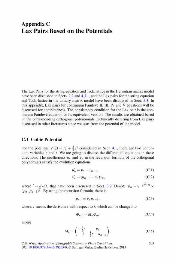
Appendix CLax Pairs Based on the Potentials
The Lax Pairs for the string equation and Toda lattice in the Hermitian matrix modelhave been discussed in Sects. 2.2 and 4.3.1, and the Lax pairs for the string equationand Toda lattice in the unitary matrix model have been discussed in Sect. 5.3. Inthis appendix, Lax pairs for continuum Painlevé II, III, IV and V equations will bediscussed for completeness. The consistency condition for the Lax pair is the con-tinuum Painlevé equation or its equivalent version. The results are obtained basedon the corresponding orthogonal polynomials, technically differing from Lax pairsdiscussed in other literatures since we start from the potential of the model.
C.1 Cubic Potential
For the potential V (z) = tz + 23z
3 considered in Sect. 4.1, there are two contin-uum variables z and t . We are going to discuss the differential equations in thesedirections. The coefficients un and vn in the recursion formula of the orthogonalpolynomials satisfy the evolution equations
u′n = vn − vn+1, (C.1)
v′n = (un−1 − un)vn, (C.2)
where ′ = d/dt , that have been discussed in Sect. 3.2. Denote Φn = e− 12V (z) ×
(pn,pn−1)T . By using the recursion formula, there is
pn,t = vnpn−1, (C.3)
where, t means the derivative with respect to t , which can be changed to
Φn,t =MnΦn, (C.4)
where
Mn =(− 1
2z vn
−1 12z− un−1
)
. (C.5)
C.B. Wang, Application of Integrable Systems to Phase Transitions,DOI 10.1007/978-3-642-38565-0, © Springer-Verlag Berlin Heidelberg 2013
203

204 C Lax Pairs Based on the Potentials
We have obtained that in the z direction, there is the following equation,
Φn,z =AnΦn, (C.6)
where
An =(−z2 − t
2 − 2vn 2vn(z+ un)
−2(z+ un−1) z2 + t2 + 2vn
)
. (C.7)
By the associated string equations,
2(un + un−1)vn = n, (C.8)
t + 2(u2n + vn + vn+1
)= 0, (C.9)
and the evolution equations given above, the un’s and vn’s can be written in termsof one variable. In terms of un, the consistency condition for the Lax pair (C.4) and(C.6) is the following continuum Painlevé II equation,
u′′n = tun + 2u3
n + n+ 1
2. (C.10)
In terms of vn, the consistency condition for the Lax pair above is the followingequation,
v′′n = (v′
n)2
2vn− 4v2
n − tvn − n2
8vn, (C.11)
which is a different version of the continuum Painlevé II equation. By using thedouble scaling given in Sect. 4.1.1, this equation can be reduced to
vξξ = v2ξ
2v− 4v2 + gv − 1
8v, (C.12)
which is close to (C.11) for n= 1, but in (C.12) g and ξ are independent. It can becalculated that
vξξ − v2ξ
2v+ 4v2 − gv + 1
8v= v
2vξ
d
dξ
(v2ξ
v+(
2v − g
2
)2
− 1
4v
)
. (C.13)
This relation indicates that the second-order equation can be reduced to the ellipticdifferential equation satisfied by the Weierstrass elliptic ℘-function discussed inSect. 4.1.2. It is obtained in Sect. 4.1.1 that
−detAn(z)= n4/3(η4 − gη2 − 2η−X+O(n−1)), (C.14)
as n is large, where z= n1/3η, g is −t/n2/3, and X is given in Sect. 4.1,
X = 1
4v−(
2v − g
2
)2
− v2ξ
v. (C.15)

C.2 Quartic Potential 205
We will discuss the differential equations satisfied by the integrals in this model inSect. D.1. The right hand side of (C.13) is corresponding to theX = 0 case discussedin Sects. 4.1.2 and D.1.
C.2 Quartic Potential
For the potential V (z) = tz2 + 14z
4 discussed by Fokas, Its and Kitaev in 1991, bythe orthogonality of the polynomials pn(z) discussed in Sect. 4.2, there is
pn,t = −vnpn + vnzpn−1, (C.16)
and the vn’s satisfy the following relations,
(2t + vn + vn−1 + vn+1)vn = n, (C.17)
v′n = vn(vn−1 − vn+1), (C.18)
where ′ = d/dt . Denote Φn = e− 12V (z)(pn,pn−1)
T . We then have the followingequation,
Φn,t =MnΦn, (C.19)
where
Mn =(− 1
2z2 − vn vnz
−z 12z
2 − vn−1
)
. (C.20)
Also, we have obtained in Sect. 4.3.1 that in the z direction there is
Φn,z =AnΦn, (C.21)
where
An =( − 1
2z3 − tz− vnz vn(z
2 + 2t + vn + vn+1)
−z2 − 2t − vn − vn−112z
3 + tz+ vnz
)
. (C.22)
The consistency condition for the Lax pair (C.19) and (C.21) is the following con-tinuum Painlevé IV equation,
v′′n = (v′
n)2
2vn+ 3
2v3n + 4tv2
n + (2t2 + n)vn − n2
2vn. (C.23)
The vn−1 and vn+1 in An and Mn can be written in terms of vn according to therelations given above. Interested readers can refer the works of Peter A. Clarksonfor more discussions on the Painlevé IV equation.

206 C Lax Pairs Based on the Potentials
C.3 Potential in the Unitary Model
Now, let us discuss the differential equation in the s direction for the potentialV (z) = s(z + z−1) explained in Sect. 6.1. Based on the discussion in Sect. 6.1 onthe unit circle |z| = 1, the equation in the s direction can be written in the followingmatrix form,
(pn,spn,s
)
=(−z−1 − xnxn+1 xn+1 + xn/z
xn+1 + zxn −z− xnxn+1
)(pnpn
)
, (C.24)
where , s means the derivative with respect to s and zpn = pn+1(z) − xn+1pn(z),where pn(z)= znpn(z) (Sect. 5.2, with γ0 = −1/2). Let
Ψn = es2 (z+z−1)
(z−n/2+1/4 0
0 z−n/2−1/4
)(pnpn
)
= es2 (z+z−1)
(χnχn
)
, (C.25)
for the (χn, χn)T in the discrete AKNS-ZS system discussed in Sect. 5.2. then wehave
Ψn,s =MnΨn, (C.26)
where
Mn =( 1
2 (z− z−1)− xnxn+1 xn+1z1/2 + xnz
−1/2
xnz1/2 + xn+1z
−1/2 − 12 (z− z−1)− xnxn+1
)
. (C.27)
In the z direction, we have obtained in Sect. 5.3.1 that
Φn,z =An(z)Φn, (C.28)
where Φn(z)= es2 (z+z−1)(z−n/2pn(z), z
n/2pn(z))T and
An =(
s2 + s
2z2 + n−2sxnxn+12z s(xn+1 − xn
z)z−1
s(xn − xn+1z) − s
2 − s
2z2 − n−2sxnxn+12z
)
. (C.29)
Since pn(z)= znpn(z), it implies Ψn and Φn have the following relation
Ψn = es2 (z+z−1)
(z−n/2+1/4 0
0 z−n/2−1/4
)(1 00 zn
)(pnpn
)
=(z1/4 0
0 z−1/4
)
Φn.
(C.30)Direct calculations show that the consistency condition Φn,zs = Φn,sz holds if thefollowing two equations hold,
x′n − 2xn+1 − xn
(n
s− 2xnxn+1
)
= 0, (C.31)
x′n+1 + 2xn + xn+1
(n+ 1
s− 2xnxn+1
)
= 0, (C.32)

C.3 Potential in the Unitary Model 207
where ′ = d/ds. These two equations are equivalent to the Toda lattice combinedwith the string equation. We are going to discuss in the following that these twoequations are a different version of the continuum Painlevé III or V equation.
Let us first consider the continuum Painlevé III equation,
Y ′ = −4Y 2Z + 2Y 2 + 2θ∞ − 1
sY − 2, (C.33)
Z′ = 4YZ2 − 4YZ − 2θ∞s
Z + θ0 + θ∞s
, (C.34)
(logW)′ = −θ0 + θ∞2sZ
+ θ0 − θ∞2s(1 −Z)
+ θ∞s, (C.35)
where Y = Y(s),Z = Z(s),′ = d/ds, and θ0, θ∞ are constants. The variablesy, z,w and t in the paper of Jimbo and Miwa (1981) are changed to −Y, sZ,W(1 − Z)1/2Z−1/2 and s respectively here. It can be verified that Y satisfies thestandard form of the continuum Painlevé III equation
Y ′′ = 1
YY ′2 − 1
sY ′ + 1
s
(αIII Y
2 + βIII)+ γIII Y
3 + δIII
Y, (C.36)
where
αIII = −4θ0, βIII = −4(1 − θ∞), γIII = 4, δIII = −4,
and Z satisfies
Z′′ = 1
2
(1
Z+ 1
Z − 1
)
Z′2 − 1
sZ′ − 1
2s2
2Z − 1
Z(Z − 1)(2θ∞Z − θ0 − θ∞)2
+ 2θ∞s2
(2θZ∞ − θ0 − θ∞)+ 8Z(1 −Z). (C.37)
Equation (C.37) can be changed to the continuum Painlevé V equation by the trans-formation Z1 = Z/(Z − 1) with t = s2,
Z′′1 =
(1
2Z1+ 1
Z1 − 1
)
Z′1
2 − 1
tZ′
1 + (Z1 − 1)2
t2
(
αV Z1 + βV
Z1
)
+ γV Z1
t
+ δV Z1(Z1 + 1)
Z1 − 1, (C.38)
where
αV = (θ0 − θ∞)2
8, βV = − (θ0 + θ∞)2
8, γV = 2, δV = 0,
and Z′1 = dZ1/dt .
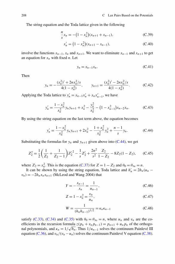
208 C Lax Pairs Based on the Potentials
The string equation and the Toda lattice given in the following
n
sxn = −(1 − x2
n
)(xn+1 + xn−1), (C.39)
x′n = (1 − x2
n
)(xn+1 − xn−1), (C.40)
involve the functions xn−1, xn and xn+1. We want to eliminate xn−1 and xn+1 to getan equation for xn with fixed n. Let
yn = xn−1xn. (C.41)
Then
yn = − (x2n)
′ + 2nx2n/s
4(1 − x2n)
, yn+1 = (x2n)
′ − 2nx2n/s
4(1 − x2n)
. (C.42)
Applying the Toda lattice to y′n = xn−1x
′n + xnx
′n−1, we have
y′n = 1 − x2
n
x2n
ynyn+1 + x2n − y2
n
x2n
− (1 − x2n−1
)xn−2xn. (C.43)
By using the string equation on the last term above, the equation becomes
y′n = 1 − x2
n
x2n
ynyn+1 + 2x2n − 1 + x2
n
x2n
y2n + n− 1
syn. (C.44)
Substituting the formulas for yn and yn+1 given above into (C.44), we get
Z′′2 = 1
2
(1
Z2+ 1
Z2 − 1
)
Z′2
2 − 1
sZ′
2 + 2n2
s2
Z2
1 −Z2− 8Z2(1 −Z2), (C.45)
where Z2 = x2n . This is the equation (C.37) for Z = 1 −Z2 and θ0 = θ∞ = n.
It can be shown by using the string equation, Toda lattice and h′n = 2hn(un −
vn)= −2hnxnxn+1 (McLeod and Wang 2004) that
Y = −xn−1
xn= 1
un−1, (C.46)
Z = 1 − x2n = vn
un, (C.47)
W = 1
(hnhn−1)1/2= κnκn−1 (C.48)
satisfy (C.33), (C.34) and (C.35) with θ0 = θ∞ = n, where un and vn are the co-efficients in the recursion formula z(pn + vnpn−1)= pn+1 + unpn of the orthogo-nal polynomials, and κn = 1/
√hn. Thus 1/un−1 solves the continuum Painlevé III
equation (C.36), and vn/(vn−un) solves the continuum Painlevé V equation (C.38).

C.3 Potential in the Unitary Model 209
The above discussions indicate that the continuum Painlevé III and V equationsare the results of the Toda lattice and the string equation. The Toda lattice and stringequation can help us to analyze the singularity of the derivatives of the free energyfunctions, that implies the continuum Painlevé equations are related to the phasetransition problems. It is discussed in Sect. 6.1 that
−z2
s2detAn = 1
4
(z+ z−1 + T
)2 − X
4, (C.49)
as n is large, where T = n/s and X is given in Sect. 6.1. We will discuss the differ-ential equations satisfied by the integrals in this model in Sect. D.2.

Appendix DHypergeometric-Type Differential Equations
In this appendix, we discuss elliptic integrals reduced from√
detAn satisfyinghypergeometric-type differential equations with an independent variable X intro-duced in the large-N asymptotics. The singularities of the hypergeometric-type dif-ferential equations can be applied to find different phases and corresponding criticalpoints in the phase transitions. The related models can be found in Sects. 4.1, 4.2,6.2 and 6.3.
D.1 Singular Points in the Hermitian Model
Based on the phase model obtained in Sect. C.1 in the Lax pair system for thecontinuum Painlevé II, let us now consider the following moment quantities in termsof the elliptic integrals,
Mj =∫
Ω
ηj√μ(η)dη, j = 0,1,2,3, (D.1)
where Ω is a cut for the μ(η) defined by
μ(η)= η4 − gη2 − 2η−X. (D.2)
Then, it can be obtained by using integration by parts that
Cd
dX
⎛
⎜⎜⎝
M0M1M2M3
⎞
⎟⎟⎠=
⎛
⎜⎜⎝
3 0 0 00 3 0 0g 0 3 03 g 0 3
⎞
⎟⎟⎠
⎛
⎜⎜⎝
M0M1M2M3
⎞
⎟⎟⎠ , (D.3)
where
C =
⎛
⎜⎜⎝
4X 6 2g 00 4X 6 2g
2gX 4g 4X+ 2g2 66X 12 + 2gX 10g 4X+ 2g2
⎞
⎟⎟⎠ . (D.4)
C.B. Wang, Application of Integrable Systems to Phase Transitions,DOI 10.1007/978-3-642-38565-0, © Springer-Verlag Berlin Heidelberg 2013
211

212 D Hypergeometric-Type Differential Equations
We want to use the singular points of the determinant of the coefficient matrix C
to find the different phases in the transition model. There would be a complicatedbackground about the relation between the roots of detC and the phases in thetransition models. The Gross-Witten model in the unitary matrix model just meetwith the singularities obtained from the corresponding hypergeometric-type differ-ential equation. In the Hermitian matrix models, the singular points obtained fromthe hypergeometric-type differential equations given below have been experiencedworking very well for the phase transition problems. There would be more inter-esting properties for the hypergeometric-type differential equations in this method,that are left for further investigations.
We want to factorize detC to find the roots, that is in fact not obvious because itis about the factorization of a polynomial in X of degree 4. However, if we changethe parameter g to a new parameter a by the following transformation,
g = 2a2 + a−1, (D.5)
obtained based on the relations of un, vn and t discussed in Sect. C.1, then theproblem becomes easier. The result is
detC = 44X(X− a + a4)(X−A(a)
)(X−B(a)
), (D.6)
where
2A(a)= −(
a4 + 3a + 1
2a−2)
+ (a2 + 2a−1)√a4 + 2a, (D.7)
2B(a)= −(
a4 + 3a + 1
2a−2)
− (a2 + 2a−1)√a4 + 2a. (D.8)
It is interesting to investigate what type of differential equation each Mj wouldsatisfy. In the following, we discuss an easy case of the elliptic integrals, andshow that the corresponding elliptic integrals satisfy the hypergeometric differen-tial equation, that indicates (D.3) is a hypergeometric-type differential equation.Denote Ω1 = [−ζ1i, ζ1i] and Ω2 = [ζ1i, ζ2i], where ζ 2
1 = (1 − √1 −X1)/2 and
ζ 22 = (1 + √
1 −X1)/2 with X1 ∈ [0,1]. Consider
I =∫
Ω
√μ1dζ, J =
∫
Ω
ζ 2√μ1dζ, (D.9)
where Ω is Ω1 or Ω2, and
μ1 = ζ 4 − ζ 2 + X1
4, (D.10)
which is obtained from another form of the Lax pair of the continuum Painlevé IIequation (Its and Novokshenov 1986). It can be verified that
(4X1 −82X1 4X1 − 8
)(I ′J ′)
=(
3 01 5
)(I
J
)
, (D.11)

D.2 Singular Points in the Unitary Model 213
where ′ = d/dX1. Then, we have
X1(1 −X1)
(I ′′J ′′)
= 1
16
(3 02 −5
)(I
J
)
. (D.12)
Therefore, I satisfies the hypergeometric differential equation
X1(1 −X1)I′′ = 3
16I. (D.13)
If one denotes I1 and I2 for I on Ω1 and Ω2 respectively, then the WronskianW(I1, I2)= I1I
′2 − I2I
′1 is a constant, that can be calculated at X1 = 0 or 1.
D.2 Singular Points in the Unitary Model
For the phase model discussed in Sect. C.3 associated with the continuum PainlevéIII, let us consider the following moment quantities,
M±j =
∫
Ω
z±j√μ(z)dz, j = 1,2, (D.14)
where
μ(η)= (z+ z−1 + T)2 −X, (D.15)
and Ω is a cut for the μ(η). Then it can be obtained by using integration by partsthat
Cd
dX
⎛
⎜⎜⎝
M−1
M+1
M−2
M+2
⎞
⎟⎟⎠=
⎛
⎜⎜⎝
−2 0 0 00 −6 0 00 0 −4 00 −2T 0 8
⎞
⎟⎟⎠
⎛
⎜⎜⎝
M−1
M+1
M−2
M+2
⎞
⎟⎟⎠ , (D.16)
where
C =
⎛
⎜⎜⎝
T 2 + 2 −X 2 4T 02 T 2 + 2 −X 3T T
3T T T 2 + 4 −X 0T T (T 2 − 1 −X) 2T 2 − 2 T 2 − 2 +X
⎞
⎟⎟⎠ . (D.17)
We have the following factorization for the determinant of the coefficient matrix forthe hypergeometric-type differential equation
detC = −X(X− T 2 − 2)(X− (T − 2)2
)(X− (T + 2)2
). (D.18)
These singular values of X are applied in Chap. 6 to discuss the phase transitionor discontinuity problems in the unitary matrix models. The cases X = 0 and X =
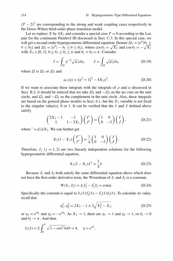
214 D Hypergeometric-Type Differential Equations
(T − 2)2 are corresponding to the strong and weak coupling cases respectively inthe Gross-Witten third-order phase transition model.
Let us replace X by 4X1 and consider a special case T = 0 according to the Laxpair for the continuum Painlevé III discussed in Sect. C.3. In this special case, wewill get a second-order hypergeometric differential equation. Denote Ω1 = {eθ |θ1 ≤θ ≤ θ2} and Ω2 = {eθ | − θ1 ≤ θ ≤ θ1}, where cos θ1 = √
X1 and cos θ2 = −√X1
with X1 ∈ [0,1], 0 ≤ θ1 ≤ θ2 ≤ π and θ1 + θ2 = π . Consider
I =∫
Ω
η−2√μ1dη, J =∫
Ω
√μ1dη, (D.19)
where Ω is Ω1 or Ω2 and
μ1(η)= (η2 + 1)2 − 4X1η
2. (D.20)
If we want to associate these integrals with the integrals of ρ and ω discussed inSect. B.2, it should be noticed that we take Ω2 and −Ω2 as the arc cuts on the unitcircle, and Ω1 and −Ω1 as the complement in the unit circle. Also, these integralsare based on the general phase models in Sect. 6.1, but the X1 variable is not fixedto the singular value(s), 0 or 1. It can be verified that the I and J defined abovesatisfy
(2X1 − 1 −1
1 1 − 2X1
)(I ′J ′)
=(
1 00 −3
)(I
J
)
, (D.21)
where ′ = d/dX1. We can further get
X1(1 −X1)
(I ′′J ′′)
= 1
4
(1 00 −3
)(I
J
)
. (D.22)
Therefore, Ij (j = 1,2) are two linearly independent solutions for the followinghypergeometric differential equation,
X1(1 −X1)I′′ = 1
4I. (D.23)
Because I1 and I2 both satisfy the same differential equation above which doesnot have the first-order derivative term, the Wronskian of I1 and I2 is a constant,
W(I1, I2)= I1I′2 − I ′
1I2 = const. (D.24)
Specifically the constant is equal to I1(1)I ′2(1)− I ′
1(1)I2(1). To calculate its value,recall that
η21, η
22 = 2X1 − 1 ± 2
√X2
1 −X1, (D.25)
or η1 = eiθ1 and η2 = −eiθ2 . As X1 → 1, there are η1 → 1 and η2 → 1, or θ1 → 0and θ2 → π . And then
I1(1)= 2∫ π
0
√1 − cos2 θdθ = 4, η = eiθ ,

D.2 Singular Points in the Unitary Model 215
I ′2(1)= 2 lim
X1→1
∫ η2
η1
dη√(η2 + 1)2 − 4X1η2
= 2 limX1→1
∫ η2
η1
dη√(η2 − η2
1)(η2 − η2
2)
.
It is the standard argument that if we make a transformation η2 = η22 + (η2
1 −η22)σ
2,then
∫ η2
η1
dη√(η2 − η2
1)(η2 − η2
2)
= 1
iη2
∫ 1
0
dσ√(1 − σ 2)(1 − k2σ 2)
,
with
k2 = 1 − k′2, k′2 = η21/η
22. (D.26)
As X1 → 1, there are η1 → 1, η2 → 1, k′ → 1 and k → 0, that imply
I ′2(1)= 2 lim
X1→1
1
iη2
∫ 1
0
dσ√(1 − σ 2)(1 − k2σ 2)
= −πi, (D.27)
and then I1(1)I ′2(1)= −4πi.
For the second term I ′1(1)I2(1), we have that as X1 → 1,
I ′1(X1)= −2
∫ −η2
η1
dη√(η2 − η2
1)(η2 − η2
2)
=O(log(η1 − η2)
),
I2(X1)=∫ η1
η2
η−2√(
η2 + 1)2 − 4X1η2dη=O(η1 − η2).
So we finally get
I1I′2 − I ′
1I2 = −4πi. (D.28)
The hypergeometric differential equations (D.12) for the Painlevé II equationand the corresponding Wronskian and conformal mappings were studied early byProfessor J. Bryce McLeod from the University of Pittsburgh. Professor McLeodguided me (Chie Bing) to get the hypergeometric differential equations (D.22) forthe Painlevé III equation discussed in my thesis at the University of Pittsburgh.The hypergeometric-type differential equations (fourth-order differential equations)discussed in this appendix are the consequence of the second-order hypergeometricdifferential equations as explained above.
The elliptic integrals and conformal mapping theory are important to study themathematical problems in the phase transition models, and there are various un-solved problems in this area. When the hypergeometric-type differential equationsare applied to other models, it should be noted that the coefficients in the μ(η) poly-nomial is generally not so simple. There may be several variables like the X variablediscussed above. The general discussion is not easy.
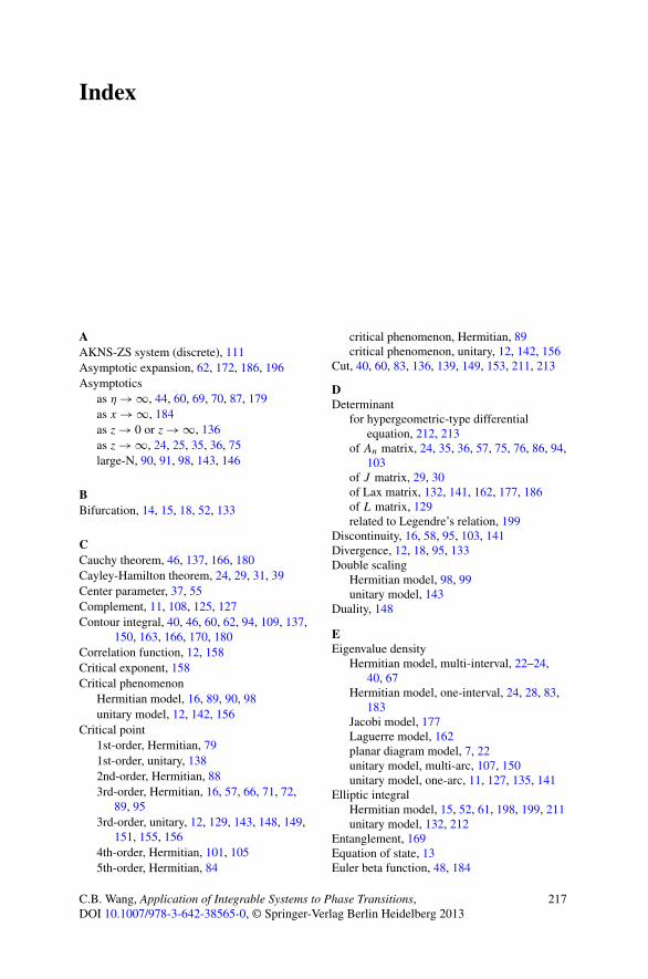
Index
AAKNS-ZS system (discrete), 111Asymptotic expansion, 62, 172, 186, 196Asymptotics
as η → ∞, 44, 60, 69, 70, 87, 179as x → ∞, 184as z→ 0 or z→ ∞, 136as z→ ∞, 24, 25, 35, 36, 75large-N, 90, 91, 98, 143, 146
BBifurcation, 14, 15, 18, 52, 133
CCauchy theorem, 46, 137, 166, 180Cayley-Hamilton theorem, 24, 29, 31, 39Center parameter, 37, 55Complement, 11, 108, 125, 127Contour integral, 40, 46, 60, 62, 94, 109, 137,
150, 163, 166, 170, 180Correlation function, 12, 158Critical exponent, 158Critical phenomenon
Hermitian model, 16, 89, 90, 98unitary model, 12, 142, 156
Critical point1st-order, Hermitian, 791st-order, unitary, 1382nd-order, Hermitian, 883rd-order, Hermitian, 16, 57, 66, 71, 72,
89, 953rd-order, unitary, 12, 129, 143, 148, 149,
151, 155, 1564th-order, Hermitian, 101, 1055th-order, Hermitian, 84
critical phenomenon, Hermitian, 89critical phenomenon, unitary, 12, 142, 156
Cut, 40, 60, 83, 136, 139, 149, 153, 211, 213
DDeterminant
for hypergeometric-type differentialequation, 212, 213
of An matrix, 24, 35, 36, 57, 75, 76, 86, 94,103
of J matrix, 29, 30of Lax matrix, 132, 141, 162, 177, 186of L matrix, 129related to Legendre’s relation, 199
Discontinuity, 16, 58, 95, 103, 141Divergence, 12, 18, 95, 133Double scaling
Hermitian model, 98, 99unitary model, 143
Duality, 148
EEigenvalue density
Hermitian model, multi-interval, 22–24,40, 67
Hermitian model, one-interval, 24, 28, 83,183
Jacobi model, 177Laguerre model, 162planar diagram model, 7, 22unitary model, multi-arc, 107, 150unitary model, one-arc, 11, 127, 135, 141
Elliptic integralHermitian model, 15, 52, 61, 198, 199, 211unitary model, 132, 212
Entanglement, 169Equation of state, 13Euler beta function, 48, 184
C.B. Wang, Application of Integrable Systems to Phase Transitions,DOI 10.1007/978-3-642-38565-0, © Springer-Verlag Berlin Heidelberg 2013
217

218 Index
FFactorization, 28, 56, 212, 213Fifth-order phase transition, 83First-order discontinuity, 16, 81, 139First-order divergence, 85Fourier transform, 191Fourth-order discontinuity, 105Free energy
Hermitian model, 7, 8, 21, 22, 45, 50–52,70, 87, 95, 191
unitary model, 11, 109, 110, 140, 141, 151,153, 157
GGross-Witten transition, 12, 110, 141, 212
HHeisenberg uncertainty inequality, 15Hermite polynomials, 2, 22Hermitian matrix model, 6, 21, 59, 132, 133Hypergeometric differential equation, 200,
213, 214Hypergeometric-type differential equation, 15,
132, 211
IIndex folding technique, 15, 26, 29Initial value problem, 49Integrable system, 30, 92
JJacobi polynomials, 3, 176, 177
LLaguerre polynomials, 161Laplace transform, 10, 183, 185Large-N transition, 15, 18, 77Lax pair
string equation, Hermitian model, 26string equation, unitary model, 116,
118–120, 124, 134, 143Toda lattice, Hermitian model, 93Toda lattice, unitary model, 133, 134
Lax pair method, 162Legendre’s relation, 199
MMarcenko-Pastur distribution, 2, 3, 162McKay’s law, 3, 177Moment quantities, 211, 213Moments, 191Multiple disjoint intervals, 9, 24, 29, 30, 39
OOrthogonal polynomials, 5, 25, 91, 110, 113,
120, 131, 208
PPainlevé equation, 204, 205, 207Partition function, 5, 10, 11, 21, 53, 103, 132Periodic reduction, 17, 30Planar diagram model, 7, 22, 73, 88Potential
Hermitian, 2, 23, 43, 55, 76, 83, 203, 205Jacobi, 179Laguerre, 162, 164unitary, 107, 120, 129, 131, 136, 148, 206
Potential parameter, 11Power-law distribution, 183
QQuantum chromodynamics (QCD), 13, 18, 91,
129, 157
RRadius parameter, 37, 55Recursion formula
four-term, 9, 15generalized Hermite polynomials, 14, 23,
24, 26Jacobi polynomials, 176Laguerre polynomials, 161, 186polynomials on unit circle, 11, 25,
110–112, 116, 122, 146, 208three-term, 6
Recursive relation, 49Renormalization, 18, 68, 91, 157Riemann-Hilbert problem, 41
SSchrödinger equation, 9, 98, 145Seiberg-Witten differential, 16, 67String equation
Hermitian model, 6, 24, 28, 92unitary model, 4, 11, 113, 114, 118, 122,
131, 141, 143, 156Strong coupling, 126, 140, 154, 155Szegö’s equation, 111, 112, 116
TThird-order divergence, 84, 89, 157, 158Third-order phase transition, 12, 52, 66, 70,
141, 153Toda lattice
Hermitian model, 5, 53unitary model, 122, 133, 207
Trace, 29, 39

Index 219
UUnified model, 1, 4, 24, 41, 162Uniform distribution, 3Unitary matrix model, 10, 108, 109, 125
VVan der Waals equation, 13Variational equation
Gross-Witten model, 108Hermitian model, 22, 50, 60, 69Jacobi model, 179, 180
Laguerre model, 162planar diagram model, 7unitary model, 107–109, 150
Von Neumann entropy, 169
WWeak coupling, 126, 129, 140, 154, 155Weierstrass elliptic function, 81, 204Wigner semicircle, 2, 183Wilson loop, 91