Causality Electromagnetic

8/12/2019 Causality Electromagnetic

http://slidepdf.com/reader/full/causality-electromagnetic 1/10

INSTITUTE OF PHYSICS PUBLISHING EUROPEAN JOURNAL OF PHYSICS

Eur. J. Phys. 25 (2004) 287–296 PII: S0143-0807(04)69749-2

Presenting electromagnetic theory in

accordance with the principle of

causality

Oleg D Jefimenko

Physics Department, West Virginia University, PO Box 6315, Morgantown,WV 26506-6315, USA

Received 1 October 2003

Published 28 January 2004Online at stacks.iop.org/EJP/25/287 (DOI: 10.1088/0143-0807/25/2/015)

Abstract

A methodof presenting electromagnetictheoryin accordancewiththe principleof causality is described. Two ‘causal’ equations expressing time-dependentelectric and magnetic fields in terms of their causative sources by meansof retarded integrals are used as the fundamental electromagnetic equations.Maxwell’s equations are derived from these ‘causal’ equations. Except for thefact that Maxwell’s equations appear as derived equations, the presentation iscompletely compatible with Maxwell’s electromagnetic theory. An importantconsequence of this method of presentation is that it offers new insights into thecause-and-effectrelations in electromagnetic phenomena and results in simpler

derivations of certain electromagnetic equations.

1. Introduction

One of the most important tasks of physics is to establish causal relations between physicalphenomena. No physical theory can be complete unless it provides a clear statement anddescription of causal links involved in the phenomena encompassed by that theory. Inestablishing and describing causal relations it is important not to confuse equations whichwe call ‘basic laws’ with ‘causal equations’. A ‘basic law’ is an equation (or a system of equations) from which we can derive most (hopefully all) possible correlations between thevarious quantities involved in a particular group of phenomena subject to the ‘basic law’. A

‘causal equation’, on the other hand, is an equation that unambiguously relates a quantityrepresenting an effect to one or more quantities representing the cause of this effect. Clearly,a ‘basic law’ need not constitute a causal relation, and an equation depicting a causal relationmay not necessarily be among the ‘basic laws’ in the above sense.

Causal relations between phenomena are governed by the principle of causality.According to this principle, all present phenomena are exclusively determined by past events.Therefore equations depicting causal relations between physical phenomena must, in general,be equationswherea present-time quantity (the effect) relates to oneor more quantities (causes)that existed at some previous time. An exception to this rule are equations constituting causal

0143-0807/04/020287+10$30.00 © 2004 IOP Publishing Ltd Printed in the UK 287

http://stacks.iop.org/EJP/25/287





288 O D Jefimenko

relations by definition; for example, if force is defined as the cause of acceleration, then theequation F = ma, where F is the force and a is the acceleration, is a causal equation bydefinition.

In general, then, according to the principle of causality, an equation between two or

more quantities simultaneous in time but separated in space cannot represent a causal relationbetween these quantities. In fact, even an equation between quantities simultaneous in timeand not separated in spacecannot represent a causal relation between these quantities because,according to this principle, the cause must precede its effect. Therefore the only kind of equations representing causal relations between physical quantities, other than equationsrepresenting cause and effect by definition, must be equations involving ‘retarded’ (previous-time) quantities.

Let us apply these considerations to the basic electromagnetic field laws. Traditionallythese laws are represented by the four Maxwell’s equations, which, in their differential form,are

∇ · D = ρ, (1)

∇ · B = 0, (2)

∇ × E = −

∂B

∂t , (3)

and

∇ × H = J +∂D

∂t , (4)

whereE is the electric field vector,D is the displacement vector,H is the magnetic field vector,B is the magnetic flux density vector,J is the currentdensity vector, andρ is the electric chargedensity. For fields in a vacuum, Maxwell’s equationsare supplemented by the two constitutiveequations,

D = ε0E (5)

and

B = µ0H, (6)

where ε0 is the permittivity of space, and µ0 is the permeability of space.Since none of the four Maxwell’s equations is defined to be a causal relation, and since

each of these equations connects quantities simultaneous in time, none of these equationsrepresents a causal relation. That is, ∇ · D is not a consequence of ρ (and vice versa), ∇ × E

is not a consequence of ∂B/∂t (and vice versa), and ∇ ×H is not a consequence of J + ∂D/∂t (and vice versa). Thus, Maxwell’s equations, even though they are basic electromagneticequations (since most electromagnetic relations are derivable from them), do not depict cause-and-effect relations between electromagnetic phenomena and leave the question of causalityin electromagnetic phenomena unanswered.

The purpose of this paper is to show how Maxwellian electromagnetic theory can bereformulated and presented in a classroom in compliance with theprinciple of causality so thatthe causal relations between fundamental electromagnetic phenomena are clearly revealed.

2. Causal equations for electric and magnetic fields

A reformulation and presentation of Maxwell’s electromagnetic theory in accordance withthe principle of causality must be based on causal electromagnetic equations that are atleast as general as Maxwell’s equations and are in complete accord with the latter. Whatshould be the form of such causal electromagnetic equations? Since an effect can be acombined or cumulative result of several causes, it is plausible that in causal equations aquantity representing an effect should be expressed in terms of integrals involving quantities



Presenting electromagnetic theory in accordance with the principle of causality 289

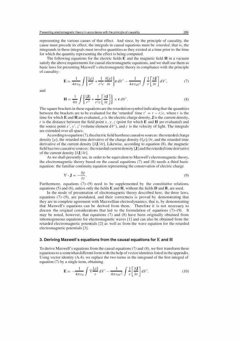
representing the various causes of that effect. And since, by the principle of causality, thecause must precede its effect, the integrals in causal equations must be retarded , that is, theintegrands in these integrals must involve quantities as they existed at a time prior to the timefor which the quantity representing the effect is being computed.

The following equations for the electric fields E and the magnetic field H in a vacuumsatisfy the above requirements for causal electromagnetic equations, and we shall use them asbasic laws for presenting Maxwell’s electromagnetic theory in compliance with the principleof causality:

E =1

4πε0

[ρ]

r 3 +

1

r 2c

∂[ρ]

∂t

r dV −

1

4πε0c2

1

r

∂J

∂t

dV , (7)

and

H =1

4π

[J]

r 3 +

1

r 2c

∂J

∂t

× r dV . (8)

The square brackets in these equations are the retardation symbol indicating that the quantitiesbetween the brackets are to be evaluated for the ‘retarded’ time t = t − r /c, where t is thetime for which E and H are evaluated, ρ is the electric charge density, J is the current density,r is the distance between the field point x , y, z (point for which E and H are evaluated) andthe source point x , y , z (volume element dV ), and c is the velocity of light. The integralsare extended over all space.

Accordingto equation (7), theelectric field hasthreecausative sources: theretarded chargedensity [ρ], the retarded time derivative of the charge density ∂ [ρ]/∂t , and the retarded timederivative of the current density [∂J/∂t ]. Likewise, according to equation (8), the magneticfield has two causative sources: the retarded currentdensity [J] andthe retarded time derivativeof the current density [∂J/∂t ].

As we shall presently see, in order to be equivalent to Maxwell’s electromagnetic theory,the electromagnetic theory based on the causal equations (7) and (8) needs a third basicequation: the familiar continuity equation representing the conservation of electric charge

∇ · J = −∂ρ

∂t

. (9)

Furthermore, equations (7)–(9) need to be supplemented by the constitutive relations,equations (5) and (6), unless only the fields E and H, without the fields D and B, are used.

In the mode of presentation of electromagnetic theory described here, the three laws,equations (7)–(9), are postulated, and their correctness is proved by demonstrating thatthey are in complete agreement with Maxwellian electrodynamics, that is, by demonstratingthat Maxwell’s equations can be derived from them. Therefore it is not necessary todiscuss the original considerations that led to the formulation of equations (7)–(9). Itmay be noted, however, that equations (7) and (8) have been originally obtained frominhomogeneous equations for electromagnetic waves [1] and can also be obtained from theretarded electromagnetic potentials [2] as well as from the wave equation for the retardedelectromagnetic potentials [3].

3. Deriving Maxwell’s equations from the causal equations for E and H

To derive Maxwell’s equations from the causal equations (7) and (8), we first transform theseequations to a somewhatdifferent formwith the help of vector identities listed in the appendix.Using vector identity (A.4), we replace the two terms in the integrand of the first integral of equation (7) by a single term, obtaining

E = −1

4πε0

∇

[ρ]

r dV −

1

4πε0c2

1

r

∂J

∂t

dV . (10)



290 O D Jefimenko

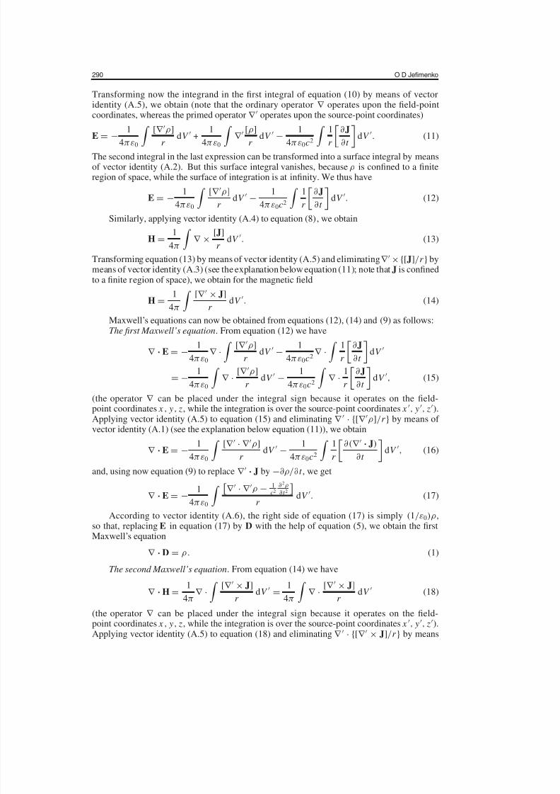
Transforming now the integrand in the first integral of equation (10) by means of vectoridentity (A.5), we obtain (note that the ordinary operator ∇ operates upon the field-pointcoordinates, whereas the primed operator ∇ operates upon the source-point coordinates)

E = −

1

4πε0 [∇ ρ]

r dV

+

1

4πε0

∇

[ρ]

r dV

−

1

4πε0c2 1

r ∂J∂t

dV

. (11)

The second integral in the last expression can be transformed into a surface integral by meansof vector identity (A.2). But this surface integral vanishes, because ρ is confined to a finiteregion of space, while the surface of integration is at infinity. We thus have

E = −1

4πε0

[∇ ρ]

r dV −

1

4πε0c2

1

r

∂J

∂t

dV . (12)

Similarly, applying vector identity (A.4) to equation (8), we obtain

H =1

4π

∇ ×

[J]

r dV . (13)

Transforming equation (13) by means of vector identity (A.5) and eliminating ∇ × {[J]/r } bymeans of vector identity (A.3) (see the explanation below equation (11); note that J is confined

to a finite region of space), we obtain for the magnetic field

H =1

4π

[∇ × J]

r dV . (14)

Maxwell’s equations can now be obtained from equations (12), (14) and (9) as follows:The first Maxwell’s equation. From equation (12) we have

∇ · E = −1

4πε0

∇ ·

[∇ ρ]

r dV −

1

4πε0c2∇ ·

1

r

∂J

∂t

dV

= −1

4πε0

∇ ·

[∇ ρ]

r dV −

1

4πε0c2

∇ ·

1

r

∂J

∂t

dV , (15)

(the operator ∇ can be placed under the integral sign because it operates on the field-point coordinates x , y, z, while the integration is over the source-point coordinates x , y , z).

Applying vector identity (A.5) to equation (15) and eliminating ∇ · {[∇ ρ]/r } by means of vector identity (A.1) (see the explanation below equation (11)), we obtain

∇ · E = −1

4πε0

[∇ · ∇ ρ]

r dV −

1

4πε0c2

1

r

∂(∇ · J)

∂t

dV , (16)

and, using now equation (9) to replace ∇ · J by −∂ρ/∂ t , we get

∇ · E = −1

4πε0

∇ · ∇ ρ − 1

c2

∂2ρ

∂ t 2

r

dV . (17)

According to vector identity (A.6), the right side of equation (17) is simply (1/ε0)ρ,so that, replacing E in equation (17) by D with the help of equation (5), we obtain the firstMaxwell’s equation

∇ · D

= ρ. (1)The second Maxwell’s equation. From equation (14) we have

∇ · H =1

4π∇ ·

[∇ × J]

r dV =

1

4π

∇ ·

[∇ × J]

r dV (18)

(the operator ∇ can be placed under the integral sign because it operates on the field-point coordinates x , y, z, while the integration is over the source-point coordinates x , y , z).Applying vector identity (A.5) to equation (18) and eliminating ∇ · {[∇ × J]/r } by means




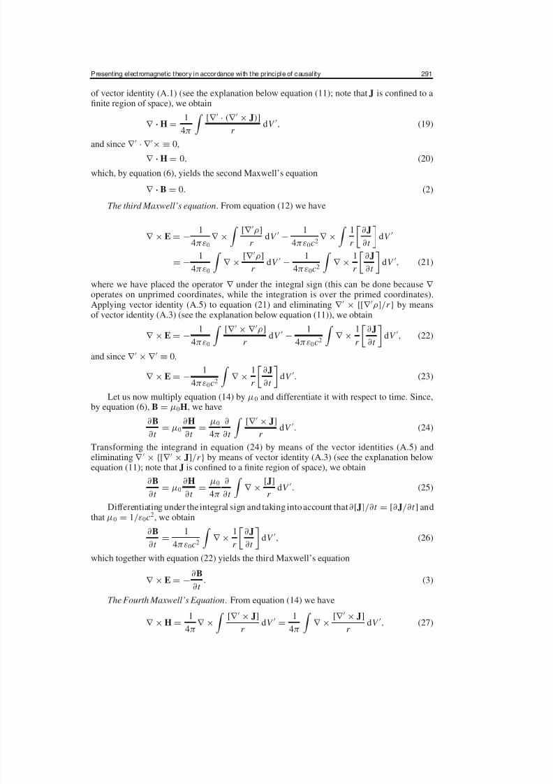
of vector identity (A.1) (see the explanation below equation (11); note that J is confined to afinite region of space), we obtain

∇ · H =1

4π

[∇ · (∇ × J)]

r dV , (19)

and since ∇ · ∇ × ≡ 0,

∇ · H = 0, (20)

which, by equation (6), yields the second Maxwell’s equation

∇ · B = 0. (2)

The third Maxwell’s equation. From equation (12) we have

∇ × E = −1

4πε0

∇ ×

[∇ ρ]

r dV −

1

4πε0c2∇ ×

1

r

∂J

∂t

dV

= −1

4πε0

∇ ×

[∇ ρ]

r dV −

1

4πε0c2

∇ ×

1

r

∂J

∂t

dV , (21)

where we have placed the operator ∇ under the integral sign (this can be done because ∇ operates on unprimed coordinates, while the integration is over the primed coordinates).Applying vector identity (A.5) to equation (21) and eliminating ∇ × {[∇ ρ]/r } by meansof vector identity (A.3) (see the explanation below equation (11)), we obtain

∇ × E = −1

4πε0

[∇ × ∇ ρ]

r dV −

1

4πε0c2

∇ ×

1

r

∂J

∂t

dV , (22)

and since ∇ × ∇ ≡ 0,

∇ × E = −1

4πε0c2

∇ ×

1

r

∂J

∂t

dV . (23)

Let us now multiply equation (14) by µ0 and differentiate it with respect to time. Since,by equation (6), B = µ

0H, we have

∂B

∂t = µ0

∂H

∂t =

µ0

4π

∂

∂t

[∇ × J]

r dV . (24)

Transforming the integrand in equation (24) by means of the vector identities (A.5) andeliminating ∇ × {[∇ × J]/r } by means of vector identity (A.3) (see the explanation belowequation (11); note that J is confined to a finite region of space), we obtain

∂B

∂t = µ0

∂H

∂t =

µ0

4π

∂

∂t

∇ ×

[J]

r dV . (25)

Differentiating under the integral sign and taking intoaccount that∂[J]/∂t = [∂J/∂t ] andthat µ0 = 1/ε0c2, we obtain

∂B

∂t =

1

4πε0

c2 ∇ ×1

r

∂J

∂t

dV , (26)

which together with equation (22) yields the third Maxwell’s equation

∇ × E = −∂B

∂t . (3)

The Fourth Maxwell’s Equation. From equation (14) we have

∇ × H =1

4π∇ ×

[∇ × J]

r dV =

1

4π

∇ ×

[∇ × J]

r dV , (27)



292 O D Jefimenko

where we have placed the operator ∇ under the integral sign (this can be done because ∇ operates on unprimed coordinates, while the integration is over the primed coordinates).Applying vector identity (A.5) to equation (27) and eliminating ∇ × {[∇ × J]/r } by meansof vector identity (A.3) (see the explanation below equation (11); note that J is confined to a

finite region of space), we obtain

∇ × H =1

4π

[∇ × (∇ × J)]

r dV . (28)

Let us now find the time derivative of D by using equation (12). Since, by equation (5),D = ε0E, we have

∂D

∂t = ε0

∂E

∂t = −

1

4π

∂

∂t

[∇ ρ]

r dV −

1

4πc2

∂

∂t

1

r

∂J

∂t

dV

= −1

4π

∇

∂ρ

∂ t

r

dV −1

4πc2

1

r

∂2J

∂t 2

dV (29)

and, making use of the continuity equation, equation (3), we obtain

∂D

∂t =

1

4π [∇ (∇ · J)]

r dV

−1

4πc2 1

r ∂

2J

∂t 2

dV

. (30)

Next, let us subtract equation (30) from (28). Placing the derivative ∂D/∂t on the right sideof the resulting equation and replacing the three integrals by a single integral, we obtain

∇ × H = −1

4π

∇ (∇ · J) − ∇ × (∇ × J) − 1

c2

∂2J

∂ t 2

r

dV +∂D

∂t . (31)

But, according to vector identity (A.7), the first term on the right in equation (30) is simplythe current density J. Replacing this term by J, we obtain the fourth Maxwell’s equation

∇ × H = J +∂D

∂t . (4)

4. Discussion

Although the presentation of electromagnetic theory on the basis of the causal equationsfor electric and magnetic fields, equations (7) and (8), is somewhat more complex thanthe traditional presentation based directly on Maxwell’s equations, such a presentation, aswe shall presently see, simplifies the derivation of some electromagnetic formulae, offersimportant new insights into certain electromagnetic phenomena and dispels certain erroneousviews on electromagnetic cause-and-effect relations. In particular, as is explained below,the presentation based on the causal electromagnetic equations shows that the traditionalexplanation of the very important phenomenon of electromagnetic induction is incorrect andreinforces the original explanation of this phenomenon provided by Faraday and Maxwell.

But let us first demonstrate how the presentation of electromagnetic theory basedon the causal electromagnetic equations simplifies the derivation of some representativeelectromagnetic formulae.

To start with, let us note that in time-independent systems there is no retardation and the

time derivatives vanish. Therefore, for time-independentsystems we immediatelyobtain fromequation (7) the Coulomb field equation,

E =1

4πε0

ρ

r 3r dV , (32)

and from equation (8) we immediately obtain the Biot–Savart law,

H =1

4π

J

r 3 × r dV . (33)




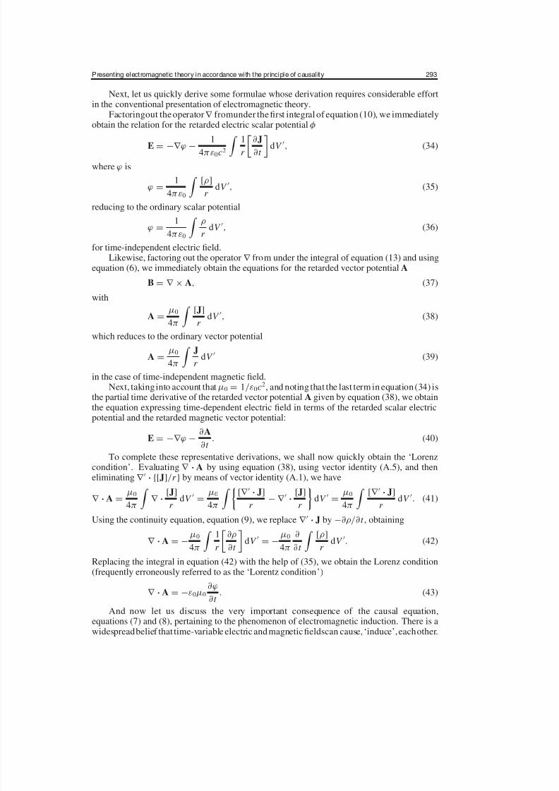
Next, let us quickly derive some formulae whose derivation requires considerable effortin the conventional presentation of electromagnetic theory.

Factoringout theoperator ∇ fromunder thefirst integral of equation (10), we immediatelyobtain the relation for the retarded electric scalar potential φ

E = −∇ ϕ − 14πε0c2

1

r

∂J∂t

dV , (34)

where ϕ is

ϕ =1

4πε0

[ρ]

r dV , (35)

reducing to the ordinary scalar potential

ϕ =1

4πε0

ρ

r dV , (36)

for time-independent electric field.Likewise, factoring out the operator ∇ from under the integral of equation (13) and using

equation (6), we immediately obtain the equations for the retarded vector potential A

B = ∇ × A, (37)

with

A =µ0

4π

[J]

r dV , (38)

which reduces to the ordinary vector potential

A =µ0

4π

J

r dV (39)

in the case of time-independent magnetic field.Next, takinginto account thatµ0 = 1/ε0c2, and noting that the last term in equation(34) is

the partial time derivative of the retarded vector potential A given by equation (38), we obtainthe equation expressing time-dependent electric field in terms of the retarded scalar electric

potential and the retarded magnetic vector potential:

E = −∇ ϕ −∂A

∂t . (40)

To complete these representative derivations, we shall now quickly obtain the ‘Lorenzcondition’. Evaluating ∇ · A by using equation (38), using vector identity (A.5), and theneliminating ∇ · {[J]/r } by means of vector identity (A.1), we have

∇ · A =µ0

4π

∇ ·

[J]

r dV =

µ0

4π

[∇ · J]

r − ∇ ·

[J]

r

dV =

µ0

4π

[∇ · J]

r dV . (41)

Using the continuity equation, equation (9), we replace ∇ · J by −∂ρ/∂t , obtaining

∇ · A = −µ0

4π

1

r

∂ρ

∂t

dV = −

µ0

4π

∂

∂t

[ρ]

r dV . (42)

Replacing the integral in equation (42) with the help of (35), we obtain the Lorenz condition(frequently erroneously referred to as the ‘Lorentz condition’)

∇ · A = −ε0µ0

∂ϕ

∂t . (43)

And now let us discuss the very important consequence of the causal equation,equations (7) and (8), pertaining to the phenomenon of electromagnetic induction. There is awidespreadbelief that time-variable electric andmagneticfieldscan cause,‘induce’,eachother.



294 O D Jefimenko

It is traditionallyasserted that, according to Maxwell’s equation (3), a changing magnetic fieldproduces an electric field (‘Faraday induction’) and that, according to Maxwell’s equation (4),a changing electric field produces a magnetic field (‘Maxwell induction’). The very usefuland successful method of calculating induced voltage (emf) in terms of changing magnetic

flux appears to support the reality of Faraday induction. And the existence of electromagneticwaves appears to support the reality of both Faraday induction and Maxwell induction. Note,however, that as explained in section 1, Maxwell’s equation (3), which is usually consideredas depicting Faraday induction, does not represent a cause-and-effect relation because in thisequation theelectricand themagnetic field is evaluated for thesame momentof time. Note alsothat in electromagnetic waves electric and magnetic fields are in phase, that is, simultaneousin time, and hence, according to the principle of causality (which states that the cause alwaysprecedes its effect), the two fields cannot cause each other (by the principle of causality, thefields should be out of phase if they create each other).

Maxwell’s equations by themselves do not provide an answer to whether or not the‘Faraday induction’ or ‘Maxwell induction’ are real physical phenomena. In Maxwell’sequations electric and magnetic fields are linked together in an intricate manner, and neitherfield is explicitly represented in terms of its sources. It is true, of course, that wheneverthere exists a time-variable electric field, there also exists a time-variable magnetic field. This

follows from ourequations (7) and (8)as well as from Maxwell’s equations (3)and (4). But, asalready mentioned, according to the causality principle, Maxwell’s equations do not reveal acausal link between electric andmagnetic fields. On theother hand, equations(7)and(8) showthat in time-variable systems electric and magnetic fields are always created simultaneously,because these fields have a common causative source: the changing electric current [∂J/∂t ](the last term of equation (7) and the last term in the integral of equation (8)).

It is important to note that neither Faraday (who discovered the phenomenon of electromagnetic induction) nor Maxwell (who gave it a mathematical formulation) explainedthis phenomenon as the generation of an electric field by a magnetic field (or vice versa).

After discovering the electromagnetic induction, Faraday wrote in a letter of November29, 1831, addressed to his friend Richard Phillips [4]:

‘When an electric current is passed through one of two parallel wires it causes at first acurrent in the same direction throughthe other, but this induced currentdoes not last a moment

notwithstanding the inducing current (from the Voltaic battery) is continued. . ., but when thecurrent is stopped then a return current occurs in the wire under induction of about the sameintensity and momentaryduration but in the opposite direction to that first found. Electricity incurrents therefore exerts an inductive action like ordinary electricity (electrostatics, ODJ) butsubject to peculiar laws: the effects are a current in the same direction when the induction isestablished, a reverse current when the induction ceases and a peculiar state in the interim. . ..’

Quite clearly, Faraday speaksof an inducingcurrent , and not atall ofan inducingmagnetic field . (In thesame letterFaraday referredto theinductionby magnets asa ‘verypowerfulproof’of the existence of Amperian currents responsible for magnetization.)

Similarly, Maxwell wrote in his Treatise [5]:‘It is only since the definitions of electromotive force. . . and its measurement have been

made more precise, that wecanenunciatecompletely thetrue law ofmagneto-electric inductionin the following terms: the total electromotive force acting round a circuit at any instant ismeasured by the rate of decrease of the number of lines of magnetic force which pass through

it. . .. Instead of speaking of the number of lines of magnetic force, we may speak of themagnetic induction through the circuit, or the surface integral of magnetic induction extendedover any surface bounded by the circuit.’

As we see, Maxwell, too, considered the electromagnetic induction as a phenomenon inwhich a current (or electromotive force) is induced in a circuit, but not as a phenomenon inwhich a changing magnetic field causes an electric field. He clearly says that the inducedelectromotive force is measured by, not caused by, the changing magnetic field. Just likeFaraday, he made no allusion to any causal link between magnetic and electric fields.




Andthere is one more fact that supports the conclusion that what we call ‘electromagneticinduction’ is not the creation of one of the two fields by the other. In the covariant formulationof electrodynamics, electric and magnetic fields appear as components of one single entity—the electromagnetic field tensor. Quite clearly, a component of a tensor cannot be a cause of

another component of the same tensor, just like a component of a vector cannot be a cause of another component of the same vector.We must conclude therefore that the true explanation of the phenomenon of

electromagnetic induction is provided by the causal electromagnetic equations, equations (7)and(8). According to these equations, in time-variable systems electric andmagnetic fields arealways created simultaneously, because they have a common causative source: the changingelectric current [∂J/∂t ]. Once created, the two fields coexist from then on without any effectupon each other. Hence electromagnetic induction as a phenomenonin which one of the fieldscreates the other is an illusion. The illusion of the ‘mutual creation’ arises from the factsthat in time-dependent systems the two fields always appear prominently together, while theircausative sources (the time-variable current in particular) remain in the background1.

Thus, even though a presentation of electromagnetic theory on the basis of the causalelectromagnetic equations is somewhat more complicated than the traditional presentation onthe basis of Maxwell equations, such a presentation is well justified by the new possibilities

that it offers and by the important new results revealed by it.

Appendix

Vector identities

In the vector identities listed below, U is a scalar point function; V is a vector point function; X is a scalar or vector point function of primed coordinates (source-point coordinates) andincorporates an appropriate multiplication sign (dot or cross for vectors); the operator ∇

operates upon unprimed coordinates (field-point coordinates); the operator ∇ operates uponprimed coordinates (source-point coordinates).

Identities for the calculation of surface and volume integrals

∇ · A dV =

A · dS (Gauss’s theorem) (A.1)

∇ U dV =

U dS (A.2)

∇ × A dV = −

A × dS. (A.3)

Identities for operations with retarded quantities

r[ X ]

r 3 +

r

r 2c

∂ X

∂t

= −∇

[ X ]

r (A.4)

∇ [ X ]

r =

[∇ X ]

r − ∇

[ X ]

r (A.5)

U = −1

4π

∇ · ∇ U − 1c2 ∂

2

U ∂ t 2

r dV (A.6)

A = −1

4π

∇ (∇ · A) − ∇ × (∇ × A) − 1

c2∂2A

∂ t 2

r

dV . (A.7)

1 The author has been unable to determine by whom, where and why it was first suggested that changing electric andmagnetic fields create each other. One thing appears certain however—the idea did not originate with either Faradayor Maxwell.



296 O D Jefimenko

References

[1] Jefimenko O D 1989 Electricity and Magnetism 2nd edn (Star City: Electret Scientific) pp 514–6 (the samepagesin the first edition of the book (Appleton-Century-Crofts, New York, 1966))

[2] Rosser W G V 1997 Interpretation of Classical Electromagnetism (Dordrecht: Kluwer) pp 82–4

[3] Jackson J D 1999 Classical Electrodynamics 3rd edn (New York: Wiley) pp 243–7[4] Thompson S P 1898 Michael Faraday, His Life and Work (New York: Macmillan) p 115, 116[5] Maxwell J C 1891 A Treatise on Electricity and Magnetism 3rd edn, vol 2 (New York: Dover) pp 176–7 (reprint)

Documents

Causality Electromagnetic