Categorical Consideration

Theory, Evidence and Market Implications

Tom Chang1

November 15, 2008

1Massachusetts Institute of Technology, Department of Economics, E52, 50 Memorial Drive,Cambridge, MA, 02142. email:tyc@mit.edu. I am especially indebted to Glenn Ellison, SendhilMullainathan and Nancy Rose. I would also like to thank Abhijit Banerjee, Sara Ellison, MireilleJacobson, and participants at the MIT Industrial Organization and Theory lunches and workshopsfor their comments.

Abstract

A growing body of evidence documents individual behavior that is difficult to reconcile withstandard models of rational choice, and firm behavior difficult to reconcile with rationalmarkets. In this paper I present a boundedly rational model of choice that reconciles severalbehavioral anomalies, and provides micro-foundational support for some puzzling empiricalregularities in firm behavior. If the evaluation of an alternative is costly, individuals mayfind it inefficient to compare all available alternatives. Instead, when faced with an unfea-sibly large choice set, some individuals may compare groups of alternatives (i.e. categories)to reduce the choice set into a more manageable set of relevant alternatives. I call theseindividuals categorical considerers and develop a model in which these decision makers se-quentially apply a single well-behaved preference relation at different levels of aggregation.I explore the implications of this model for both individual behavior and equilibrium firmbehavior in market settings. Under certain conditions, the existence of categorical consid-erers in a market causes firms to utilize strategies different from what would be optimalin a market of fully rational consumers. This simple model generates predictions aboutbehavior consistent with several new field experiments, and offers possible explanations forexcess spatial product differentiation, brand name premiums, and product branding.

1 Introduction

A growing body of literature documents individual behaviors that are difficult to reconcile

with standard models of rational choice. Some of the most compelling of these studies

show dramatic changes in consumer behavior in response to changes in the decision-making

environment that, according to the standard model, should be either unimportant or un-

informative.1 Similarly, a new but growing literature in Boundedly Rational Industrial

Organization (BRIO) examines firm behavior difficult to reconcile with rational markets.2

In this paper, I present a model of discrete choice that serves to reconcile several es-

tablished behavioral anomalies in a boundedly rational framework. This model is based on

the idea that if product evaluation requires time and other cognitive costs, consumers may

find it infeasible or undesirable to compare all available alternatives. When faced with an

infeasibly large choice set, consumers utilize categorical comparisons to quickly reduce the

choice set into a more manageable set of relevant alternatives. I refer to this process as

categorical consideration.

I show that this model reconciles several behavioral anomalies in a parsimonious, wel-

fare preserving manner. In addition the model provides a micro-foundation for several

empirical regularities in firm behavior, including excess product differentiation, premiums

for physically identical products, certain types of pay-for-placement, and artificial product

differentiation through branding.3

In my model, boundedly rational consumers sequentially apply a single well-behaved

preference relation at different levels of aggregation. This model retains the assumption

that consumers have stable preferences, but relaxes the assumption that they are applied

simultaneously over all alternatives. Instead consumers first utilize categories to reduces the

set of available alternatives to a smaller set of “relevant” alternatives, and then select their

preferred alternative from this limited set. Borrowing a term from the marketing literature,1See Simonson (1989), McFadden (1999), Iyengar & Lepper (2000), Boatwright & Nunes (2001), Poilaine

(2006), and Chang, Mullainathan & Shafir (2008).2For examples see Della Vigna & Malmendier (2004, 2005), Heidhues & Koszegi (2005, 2008), Eliaz and

Spiegler (2006), Spiegler (2006a 2006b) and Mullainathan et al. (2008). Ellison (2006) also provides anexcellent recent overview of the BRIO literature.

3Real product differentiation refers to firms producing different product varieties, while ‘artificial’ productdifferentiation refers to a firm’s use of branding to generate the appearance of increased variety (i.e. productthat vary only in terms of non-informational labels).

1

I refer to this set of relevant alternatives as the consideration set.4 The core of my model is

the process by which consumers use categories to reduce the set of available alternatives into

a consideration set. When faced with an infeasibly large number of alternatives, consumers

first divide the alternatives into categories. Consumers then choose the preferred good from

the alternatives in their preferred category.

For concreteness, imagine the decision process of an individual deciding where to go for

dinner. In both the standard and categorical consideration models, the decision maker is

assumed to have a stable system of preferences over attributes and knows (or has access

to) the attributes of a large number of restaurants. In the standard model, a consumer

would fully evaluate all available restaurants and select the utility-maximizing one. In

contrast a categorical considerer first decides on the type of cuisine she wants (e.g. pizza,

Chinese, seafood) and then chooses the utility maximizing restaurant from the subset of

restaurants in her preferred category. The main insight of categorical consideration is that

when individuals use coarse partitions to eliminate a set of alternatives, individual choice

can be affected by both the overall composition of the choice set (i.e. irrelevant alternatives)

and how the choice set is partitioned (i.e. what categories an individual uses).

A categorical consumer’s choice procedure then proceeds in two stages. First, if faced

with “too large” a set of alternatives, individuals use ` to partition the set S into subsets

{Sm}. In the first stage categorical consumers choose their preferred subset Sm∗ from {Sm}.

Decision makers then proceed to the second stage in which they select their preferred object

j∗ from the consideration set C ≡ Sm∗.

Put another way, for an alternative to be chosen not only must it be preferred to other

alternatives in its category, but it’s category must also be preferred to all other categories.

That is, demand for a good j in S is jointly determined by the demand for good j relative

to other goods in its category, as well as the demand for its category relative to the other

categories in S.

Though categorical consideration retains the assumption that individuals have a single

set of stable preferences over characteristic bundles, the sequential application of these

preferences at different levels of aggregation generates choice behavior inconsistent with4See Roberts and Lattin (1997) for an review of the marketing research on consideration sets.

2

the standard model. Three implications of this process generate the non-classical behavior

- coarseness, limited consideration, and framing.

In the first stage of categorical consideration, instead of separately evaluating all avail-

able alternatives, consumers sort alternatives into aggregations of similar objects. That

there are fewer partitions than distinct alternatives is what I refer to as coarseness or cat-

egorical thinking.5 Coarseness is then equivalent to a rational individual who is simply

unable to distinguish between distinct alternatives within a category.

Limited consideration refers to the fact that individuals select their preferred alternative

from alternatives in their consideration set. That is, they only seriously consider products in

their preferred category. When the consideration set is the full set of alternatives (C = S),

the model is equivalent to the standard rational model. But when the consideration set is

strictly smaller than the full set of alternatives (C ⊂ S), limited consideration can clearly

lead to choice behavior different from the rational baseline.

Framing deals with the fact that a set of alternatives may be divisible or categorizable

in more than one way. Since the effect of both coarseness and limited consideration de-

pends on the specific categories used, the dimension by which S is subdivided into distinct

categories is an important determinant of consumer choice over S. I refer to the specific

subdivision as a “frame.” Each distinct ` then specifies a particular frame in which cate-

gorical consideration takes place. For the remainder of the paper, framing or the framing

effect refers to the overall impact of a particular ` on consumer choice.

In this paper, I largely limit myself to exogenously determined frames. A study of

endogenous framing is an important area for future work. Following a brief literature

review, the paper proceeds in four parts. In Section 2 I present the categorical consideration

model and highlight some of the key implications of the model for consumer behavior.

In Section 3 I present the results of three recent field experiments that provide empirical

support for the model. The first experiment focuses on the impact of coarseness on demand

for a differentiated product (i.e. single serving lunch options at a local market). Consistent5This is a slight abuse of a term from Mullainathan (2000), where coarse thinking refers to a model of

human inference in which instead of continuously updating their priors based on the Bayesian idea, peoplehave only a finite number of priors or mental categories. In my model, coarseness refers to the idea thatdecision makers do not differentiate between the full set of alternatives, but instead make evaluations basedon aggregations of alternatives (i.e. categories).

3

with my model, I find that putting a good on sale increases the sale of substitute goods in

the same category as the sale item. I next show how standard methods for the structural

estimation of discrete-choice models can be modified to account for the presence of some

categorical consumers. Applying these methods to the data, I find that a model with

some categorical consumers has better predictive power than the standard model. The

second experiment highlights the impact of limited consideration. Specifically I find that

mixing bottles of water that were previously in adjacent but separate coolers changes brand

market share by a factor of 14. The third experiment examines the importance of frames of

categories in determining choice. I find that providing consumers with informative labels

categorizing jars of jam decreases aggregate demand across three bakeries.

In Section 4, I examine profit maximizing firm behavior in several market settings and

show how equilibrium strategies are affected by the presence of some categorical consumers.

I first show that in the presence of categorical consumers, a monopolist has an incentive

to produce greater variety. Then in a sequential entry setting, I show that incumbents

can credibly deter entry through pre-emptive investment in new goods (i.e. crowding the

product space). Both these results suggest that the presence of categorical consumers

can bias a market toward multi-product monopoly. In the third market application, I

show how the presence of categorical consumers can explain how multi-product brands

are able to maintain price premiums over physically identical generic goods. In the final

market application I show how firms may be able to decrease competition by artificially

differentiating their product through product branding.

Section 5 concludes.

1.1 Literature Review

The model presented in the paper is a synthesis of two different literatures on bounded ratio-

nality - the marketing literature on consideration sets and the literature in both psychology

and economics on categorical thinking.

The marketing literature on consideration sets dates back to Miller (1956), and takes

many of its cues from an even older psychology literature regarding the ability of consumers

to evaluate a large number of alternatives. The basic ideas behind consideration sets are

4

that in many real world settings, individuals are offered a myriad of alternatives and that

because of either psychological constraints or cognitive costs, considering all the possible

alternatives is either infeasible or inefficient. Consumers therefore seriously consider only a

small set of alternatives, ignoring the rest.

The earliest literature tended to focus on demonstrating that, for various specifications

of cognitive costs, the evaluation of all available alternatives is non-optimal.6 More recently,

the marketing literature has moved their focus to the implications of consideration sets on

aggregate behavior (Hauser and Wernerfelt 1990) and on consideration set formation itself

(Tversky & Sattath 1979, Chakravarti & Janiszewski 2003). For example, in Roberts

and Lattin (1991), the authors find a closed form solution for the number of “brands” an

individual would consider as a function of evaluation costs and expected distribution of

utilities for brands. Chakravarti and Janiszewski (2003) model consumers as constructing

consideration sets by including products that are highly “alignable” or have a high number

of overlapping features.

The concept of categorical thinking - that decision makers process information with the

aid of categories - dates back to the social psychology literature of the 1950s.7 Most often

applied in the context of stereotypes, social psychologists have generated a significant body

of work demonstrating the important role categories play in individual decision making. In

linguistics the idea of a type of categorical thinking is implicitly the basis for the debate

of whether or not structural variation in language lead to qualitative spatial variation in

perception, or more simply stated whether language impacts how individuals perceive the

world around them.8

More recently, economists have looked to categorical thinking as a means of understand-

ing choice behavior. Mullainathan (2002) and Fryer & Jackson (2007) present models of

human inference where decision makers have fewer mental categories than actual varieties,

and explore how such categorization affects decision making. Mullainathan et al. (2008)

explores how such thinking can be exploited by persuaders to shed light on how uninfor-6Examples include Shugan (1980), Ratchford (1980), Roberts (1983), and Roberts & Lattin (1991).7Ashby & Maddox (1993), Reed 1972, Roscho 1978, Rosseel 2002, Brewer 1998, Bruner 1957, Macrae &

Bodenhausen (2000), Lepore & Brown (1997), Kreiger (1995), Bargh (1999), Quinn & Eimas (1996).8See for example Hayward & Tarr (1994).

5

mative messages can affect beliefs. Of a more theoretical bent, Ellison & Holden (2008)

examine a model with endogenously coarse rules and Peski (2007) presents a model of se-

quential learning in which, under certain conditions, dividing objects into categories with

similar properties is part of an optimal solution. My model is very much in the general

spirit of this more recent literature, and can be thought of as a consideration set model of

choice where consideration sets are formed through categorical thinking.

My model of categoric consideration is also closely related to the choice-theoretic lit-

erature on sequential decision making. Since categorical designation is based on product

attributes, the first stage of categorical decision making has clear similarities with the Elim-

ination by Aspects theory of choice (Tversky (1972)). In terms of two stage decision pro-

cesses, Mariotti and Manzini (2008) present a model of Sequentially Rationalizable Choice

called the Rational Shortlist Method (RSM) in which consumers first reduces the set of

alternatives into a shortlist. Masatlioglu and Nakajima (2008) present a general framework

of Iterative Search. According to iterative search, for each good there are a set of “relevant”

alternatives, and consumers iterate through a path-dependent set of consideration sets to

decide on an alternative. Eliaz and Spiegler (2007) present an implementation of iterative

search and explore the implications of their model on competition between two firms.

This paper also contributes to the growing body of work in boundedly rational industrial

organization. This relatively recent but fast growing body of literature studies firm behav-

ior in the face of consumers who exhibit behavior that is boundedly rational along some

dimension.9 Particularly relevant to this paper is work by Shapiro (2006), Mullainathan

et al. (2008), Carpenter et al. (1994), and Eliaz and Spiegler (2007), who explore ways

in which non-informational advertising can influence the behavior of boundedly rational

consumers.

Although my model shares many of the features of this choice-theoretic literature, there

are several key differences. First while individuals sequentially apply a binary preference

relation, only one preference relation is needed. That is, instead of sequentially applying

two asymmetric binary relations (the first of which may or may not correspond to a well9Examples include DellaVigna & Malmendier (2004, 2005), Ellison (2005), Gabaix & Laibson (2006),

Heidhues & Koszegi (2005, 2008), Rubinstein (2003), Schlag (2004), Spiegler (2004, 2006).

6

behaved preference relation), in my model individuals utilize a single standard preference

relation at different levels of aggregation. More significantly, unlike the iterative search

models, the model presented here does not rely on a pre-determined starting good (or

set of goods) to generate consideration sets.10 Since the predictions of an iterative search

model with endogenous reference points depend importantly on a parameter generated by

a process outside the scope of the model itself, falsification is necessarily more difficult.

In addition since the only restriction on consideration sets is that it includes the reference

product, iterative search requires the econometrician to observe the actual consideration

sets used by individuals to identify preferences.

2 Consumer Behavior

2.1 The Basic Model

Let S be a non-empty finite set of mutually exclusive alternatives indexed by j and where

each alternative can be treated as a bundle of K characteristics; that is we assume that

a product j can be fully characterized by a vector xj ∈ X where X is a K-dimensional

Euclidean space and a price pj ∈ <.

A frame is a partitioning of characteristic space X as defined by `. Then any two

alternatives j and j′ whose characteristic vectors xj and xj′ occupy the same partition in

X are grouped together. That is, categories are defined as alternatives with characteristic

vectors in a subspace xk ∈ Xm ⊂ X. Product partitions or categories are indexed by

m = 1, 2, . . . ,M and denoted by Sm. The elements of Sm are denoted as jm and indexed

from 1 to Jm.

Consumers are indexed by i and characterized by types θi ∈ Θ. Consumers have unit

demand for at most one good and always have an outside option S0 = {j0}. For an

individual of type θ, her preference over attribute bundles is then given by a function fθ

that maps a vector x ∈ X to a point on the real line, f : X 7→ <. Her utility for a given

instance of an attribute bundle is given by a sum of her preferences over attribute bundles

and a probabilistic term ηj,θ. The utility of a user of type θi if she purchases good j can

10In these models, the endogenous starting point is usually discussed in terms of a default or status quooption.

7

then be written as

ui(j, pj) = fθi(xj , p) + ηj,θi

. (1)

The utility an individual derives from an alternative j is jointly determined by a function

of its characteristics xj and a stochastic term ηj . Let S be a set of J alternatives indexed

by j. Assuming η takes on discrete values, the expected value of good j is

E(uθ(j)) =∑ηj,θi

Pr(ηj,θ = η)[fθ(xj , p) + ηj,θ] = fθ(xj , p) + E(ηj |θi).11 (2)

Since a consumer can choose only a single alternative, the utility a consumer can extract

from a set of alternatives S is equivalent to the highest utility provided by any single

alternative in S. Specifically, the utility a consumer of type θi can extract from set S is

given by

Ui(S) = Max{uθi(j, pj)} ∀j ∈ S. (3)

Since utility has a stochastic component, the value of Uθ(S) depends on the specific real-

ization(s) of ηj,θi. Let Z be a set indexed by z that corresponds to the set of all possible

values of Uθ(S), and σz be the probability that Ui(S) = Ui,z. Then before learning the

stochastic component of products’ utility, a consumer of type θi has expected utility from

set S given by

E(Ui(Sm) =∑Z

σzUi,z. (4)

Categorical consideration then proceeds as follows: A consumer uses ` to partition a set

of alternatives S into categories Sm and chooses the category S∗m with the highest expected

11Similarly when η is continuous, the analogous identity is E(uθ(j)) =R

ηj,θi

dηh(η)[fθ(xj , p) + η] =

fθ(xj , p) +R

ηj,θi

dηh(η)ηj,θi = fθ(xj , p) + E(η|θi) where h(η) is the probability distribution function forηj,θi .

8

utility. I refer to this preferred category of alternatives as the consideration set and denote

it by C. The consumer then examines the products in her consideration set (i.e. learns the

value of the stochastic component of utility) and chooses the utility maximizing alternative

j ∈ C which I denote as j∗.

Note that in the special case where C = S (i.e. S is partitioned into a single set

containing all available alternatives), the model is equivalent to the standard model of

rational choice. Deviations from the standard model occur when S is partitioned into

multiple categories.

Consider the following example, where consumers use a single ` to partition S into

multiple categories, each of which contains more than one alternative j. Categorical con-

sideration is then captured by a two step process in which consumer i first selects the

category that maximizes her expected utility (C ∈ {Sm}), and then chooses the utility

maximizing alternative (jm ∈ C).

The probability that a product j′ ∈ Sm is the preferred good is then given by the joint

probability Pr(j′ = j∗) = Pr(u(j′) > u(−j′)) ∗ Pr(U(Sm) > U(S−m)). That is, for good

j to be the chosen good, it must be both the preferred good in its category and belong to

the preferred category.

For any alternative j′ ∈ Sm the characteristics of the other alternatives −j ∈ Sm will

impact the probability of it being chosen in two ways. In a slight abuse of the notation,

we note that ∂∂u(−j′)Pr(u(j′) > u(−j′)) ≤ 0. That is, according to the first term, the

probability that j is the preferred good decreases in the utility of other goods in the set Sm.

This term is just the result of the standard substitution effect among the goods j ∈ Sm.

But because consumers select their preferred good from only among the alternatives in their

consideration set C, the probability that the good is considered at all is increasing in the

utility of the other goods in its category Sm. This effect is captured by the second term for

which ∂∂u(−j′)Pr(u(Sm) > u(S−m)) > 0. That is, the probability of a good j being chosen

increases in the utility of other goods in set Sm.

9

2.1.1 Interpreting ηi,j

The stochastic element ηi,j plays a crucial role in generating non-rational behavior. In

the special case where ηi,j = ki ∀j, the model reduces to the rational model. As such,

understanding the role of uncertainty can provide guidance as to where we would expect

to see significant departures from rationality. Specifically, we would expect significant

departures from rationality only when some aspect of product utility is uncertain.

Interpretation of the uncertainty introduced by ηi,j can perhaps be best understood in

relation to the well known Random Utility Model (RUM). In both the RUM and Categorical

Consideration Model (CCM), for a given consumer of type θi, the utility of an alternative j

is assumed to be jointly determined function of its characteristics xj and the attributes of

the consumer: ui(j) = f(xj , θi). In the RUM the stochastic component of consumer utility

is due to product characteristics unobservable to the econometrician. That is, although

individual consumers costlessly observe all product characteristics xj and behave determin-

istically, the econometrician observes only a strict subset of a product’s characteristics. The

stochastic component ηi,j simply compensates for the econometrician’s inability to observe

all the relevant parameters, and has no impact on an individual’s choice. For individual, de-

cisions are fully deterministic and only appear probabilistic to the econometrician because

of unobservables.

In contrast, under CCM, individuals costlessly observe only a subset xj of product

characteristics, and have some beliefs on the values of the remaining product characteristics

xj . Consumers can learn values of the characteristics xj . But because such learning is costly,

when faced with a large number of alternatives, consumers are unwilling to evaluate them

all individually. Instead they use the costlessly observable characteristic and their beliefs

about the unobserved product characteristics to reduce the set to a smaller number of

highly relevant alternatives to evaluate.

Consider a consumer shopping for a car. According to RUM, consumers costlessly

observe all product characteristics and can therefore determine the utility each car would

provide. A consumer then simply chooses the car that provides the utility from the full

set of available automobiles. According to CCM, consumers costlessly observe only some

10

product characteristics and have (correct) beliefs regarding the distribution of the remaining

product characteristics. Consumers then decide based on the observable characteristics and

beliefs which cars to investigate further (e.g. test drive) in order to learn the previously

unobserved product characteristics to determine a car’s actual utility.

As a second example, consider the decision process of a consumer presented with a

display free sample display for an unfamiliar brand of jam. Although the consumer may

have well defined preferences over jam flavors (e.g. she prefers strawberry to grape), she

may still face some uncertainty regarding her preferences over these specific jams - an

uncertainty that can be resolved by taking a free sample.

According to CCM, when faced with such a display, a consumer will look over all the

available alternatives (flavors) and categorize then according to some criteria (e.g. jams or

jellies, berry or citrus). The consumer then chooses her preferred category and tastes only

the jams in that category (i.e. consideration set). She purchases one of the tasted jams if

she likes it well enough.12

2.2 Implications of the Model

Under categorical consideration, bounded rationality manifests in two ways: limited con-

sideration and coarse thinking. Simply stated limited consideration says that a decision

maker does not necessarily choose from amongst the full set of available alternatives. That

is, in the presence of limited consideration, a decision maker might select an alternative

that would not have been chosen if she had evaluated all available alternatives. Coarse or

categorical thinking says that the decision maker might not treat all alternatives as dis-

tinct, but instead uses coarser partitions in which several alternatives are placed into a

single partition or category. A specific set of categories used to partition a set of goods

is referred to as a frame. These two factors combine to generate a range of behavioral

anomalies consistent with a range of both empirical studies of individual choice behavior

and observed firm strategies.12The prediction that consumers fully evaluate only a subset of available items is supported by data from

the jam tasting booth experiment in Iyengar and Lepper (2000). Though not the main thrust of theiranalysis, one striking result of their experiment is that even when faced with as many as 24 different jams,individuals tasted on average only slightly more than two samples.

11

Choice behavior under categorical consideration need not satisfy the Weak Axiom of

Revealed Choice (WARP) or equivalently the Axiom of Independence of Irrelevant Alterna-

tives (IIA). This violation can arise one of two ways. First, because of coarseness, whether

or not a good is even considered is a function of the other goods in its category. Second,

if a product’s classification (i.e. `) is endogenously determined, an irrelevant alternative

could affect the categories themselves.

As a simple example assume that a consumer uses a single frame to partition goods

such that alternatives {A,B, C} correspond to categories S1 = {A} and S2 = {B,C}. Let

A �> C � B � 0) and {B,C} � {A} � 0. Consider the the behavior of a categorical

consumer when presented with S = {A,B, C} or S′ = {A,C}.

If S = {A,B, C}, in the first stage the consumer compares product S1 = {A} to

S2 = {B,C}. Then since {B,C} � {A} � 0, the consumer will choose S2 = {B,C} as her

consideration set. And since C � B � 0, the consumer will choose alternative C. If instead

S′ = {A,C}, the consumer first compares S1 = {A} and S2 = {C}. {A} � {C} � 0 so

the consumer’s consideration set is S2 = {A}, and since A � 0 the consumer will choose

alternative A.

Unlike many characterizations of violations of WARP, the change in choice does not

arise from inconsistent preferences, but rather as a result of the sequential application

of a single, well behaved preference relation at different levels of aggregation. That is,

categorical consideration is a procedurally rational attempt to approximate fully rational

choice behavior.

When consumers are categorical, “irrelevant” alternatives affect decision making through

coarseness. In terms of utility, the condition that a products utility depends only on its own

characteristics and not that of other goods is sufficient to guarantee IIA. But in categori-

cal consideration, coarse thinking alternatives are not seen as distinct entities but instead

share the characteristics of the alternatives in the category. Therefore, though categorical

consideration does not always satisfy IIA, it specifies a (restrictive) mechanism through

which these violations are generated.

The following axioms illustrate some of the implications of these restrictions.

12

Axiom 1 Very Weak Axiom of Revealed Preference (VWARP): For any finite set of mu-

tually exclusive options S, if a decision maker chooses jm∗ in partition Sm ⊂ S, then no

j ∈ Sm 6= jm∗ will ever be the chosen good for any possible partitioning of S if its partition

includes jm∗.

This axiom arises from the fact that within categories, preference rankings of goods are

stable. That is, if a good is preferred to another good, it will always be preferred to the

other good if they are in the same category, regardless of how categories are partitioned.

An alternative specification of VWARP is that for a fixed set of partitions {Sm}, the

selected alternative is limited to the set {jm∗}. The alternative chosen by a categorical

considerer must be the best in a given category. Note that this means that although a

consumer may purchase a good that is strictly dominated by another available alternative,

categorical consideration will never lead a consumer to mistakenly purchase a good that

did not provide some consumer surplus.

Axiom 2 Weak Axiom of Revealed Categorical-Preference (WARC): Let {Sm} define a

finite partition of a set of mutually exclusive options S. If category Sx � Sy given {Sm},

then Sx � Sy given {Sm, Sk} for all Sk.

This axiom arises from the fact that consumer preferences are stable across categories.

In other words, at every stage of decision making, a categorical considerer acts rationally.

That is, for any given set of sets, the WARP holds. Violations from the standard model

are then the result of the fact that individual preference relations are applied on different

levels of aggregation.

Axiom 3 Best is Best: Let u generate a cardinal measure of preference for alternatives

j ∈ S and let u∗ correspond to the highest utility of a good in set S. For any set of goods

S, there exists a good jb with ub > u such that good jb will be chosen regardless of how S

is partitioned.

This axiom states that for any given set S, if a product is good enough, it will be selected

regardless of categorization. That is, if a product is “better enough,” consumer choice is

13

invariant to bounded rationality. Though this result may seem somewhat trivial, many

models of limited consideration do not satisfy this axiom. For example, in both the classic

consideration set model from marketing and the iterative search model, since product utility

is not necessarily used to generate the consideration set, a good need not be considered

regardless of how much better it is than the considered alternatives. Put anther way, a

fundamental property of most models of limited consideration is that consumers essentially

choose a local maxima (i.e. best good in a category). Under categorical consideration,

since the choice of consideration set (i.e. best category) is based in part on the value of

the best in class alternative, the decision maker will always choose the global maxima if it

represents a sufficiently large enough improvement over all other local maxima.

3 Empirical Examples

The following three empirical examples serve the dual purpose of grounding behind cate-

gorical consideration in real world situations and providing empirical evidence in support

of the model. The first example explores consumer behavior when a good j is replaced

by a strictly superior good j′ for a fixed set of categories. Specifically I examine aggregate

demand behavior when the price of a single good is reduced. I then show how to modify the

standard structural econometric methods to account for the presence of some categorical

consumers. In the second example both the categories and product set are fixed, but a

good j is moved from one category to another. In the final example, I examine demand

when consumers use different categories to partition a fixed set of products.

3.1 Example 1: Fixed Category Sales

In standard demand models, in the absence of complementarities and income effects (e.g.

discrete choice models commonly used in Industrial Organization), replacing a good with a

more attractive alternative cannot increase the demand for other goods. In contrast, in the

categorical consideration model, replacing a good with a more attractive alternative can

increase the demand for other (substitute) goods.

Consider the following field experiment:13 A retail store sells a variety of fresh single-13See Chang et al. (2008) for a more detailed treatment of the experimental setup.

14

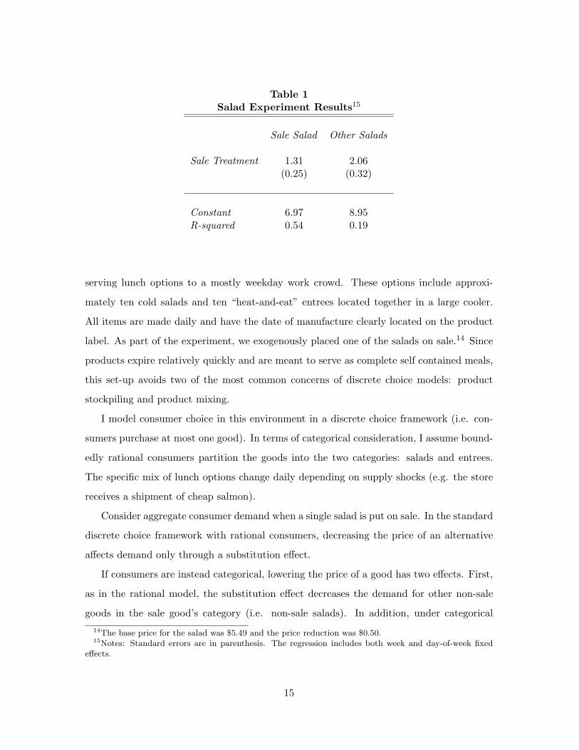
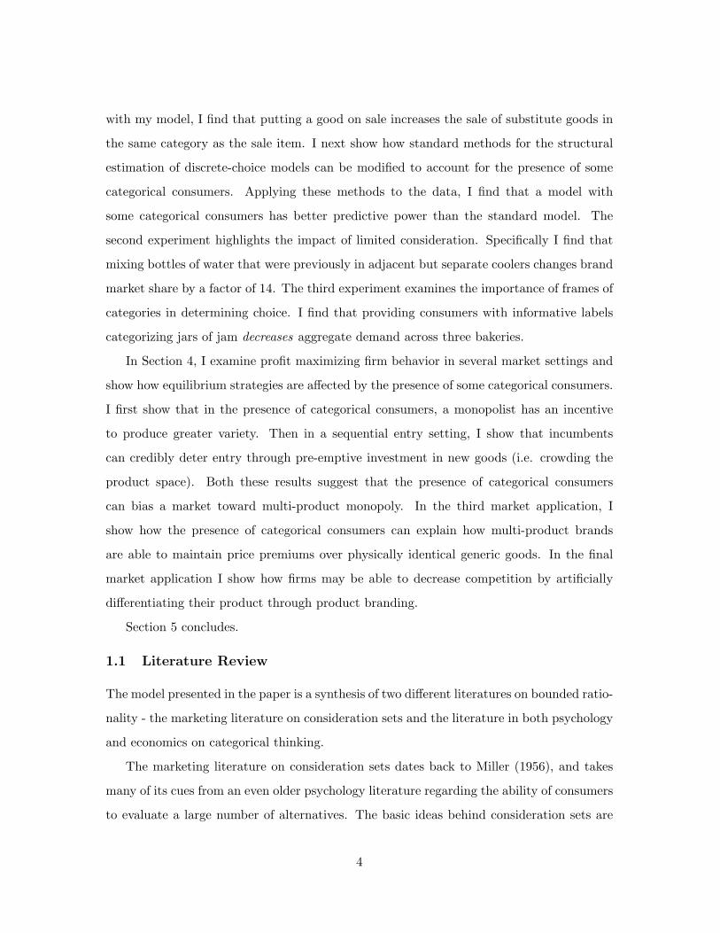
Table 1Salad Experiment Results15

Sale Salad Other Salads

Sale Treatment 1.31 2.06(0.25) (0.32)

Constant 6.97 8.95R-squared 0.54 0.19

serving lunch options to a mostly weekday work crowd. These options include approxi-

mately ten cold salads and ten “heat-and-eat” entrees located together in a large cooler.

All items are made daily and have the date of manufacture clearly located on the product

label. As part of the experiment, we exogenously placed one of the salads on sale.14 Since

products expire relatively quickly and are meant to serve as complete self contained meals,

this set-up avoids two of the most common concerns of discrete choice models: product

stockpiling and product mixing.

I model consumer choice in this environment in a discrete choice framework (i.e. con-

sumers purchase at most one good). In terms of categorical consideration, I assume bound-

edly rational consumers partition the goods into the two categories: salads and entrees.

The specific mix of lunch options change daily depending on supply shocks (e.g. the store

receives a shipment of cheap salmon).

Consider aggregate consumer demand when a single salad is put on sale. In the standard

discrete choice framework with rational consumers, decreasing the price of an alternative

affects demand only through a substitution effect.

If consumers are instead categorical, lowering the price of a good has two effects. First,

as in the rational model, the substitution effect decreases the demand for other non-sale

goods in the sale good’s category (i.e. non-sale salads). In addition, under categorical14The base price for the salad was $5.49 and the price reduction was $0.50.15Notes: Standard errors are in parenthesis. The regression includes both week and day-of-week fixed

effects.

15

consideration, the coarseness effect predicts that decreasing the price of a good increases

the attractiveness of the sale goods category. This second effect leads to an increase in the

number of consumers who choose salads as their consideration set. In terms of the demand

for non-sale salads, coarseness acts as a countervailing force to the usual substitution effect,

and can even lead to an increase in demand for non-sale salads.

Table 1 reports the sales of salad on sale and non-sale days. The first two columns of

Table 1 report the sales of the sale item under the sale and no sale condition. As predicted

by both models, reducing the price of a salad increases demand for the good. The second two

columns of Table 1 report the sales of non-sale salads under the sale and no-sale condition.

Inconsistent with rational choice, putting a salad on sale significantly increases the sales of

non-sale salads.

3.1.1 Estimation

Since categorical consideration is based on a single well behaved preference relation oper-

ating in a restrictive framework, welfare analysis and counterfactual generation is possible

using standard techniques on commonly available datasets.

To wit, consider the following example of an implementation of categorical consideration

in a random utility framework. Let ζi and wj represents the attributes of person i and char-

acteristics of product j respectively. Assuming the conditional utility for individual i from

product j is a function of individual attributes (i.e. type), ζi and product characteristics

wj we can write individual utility as

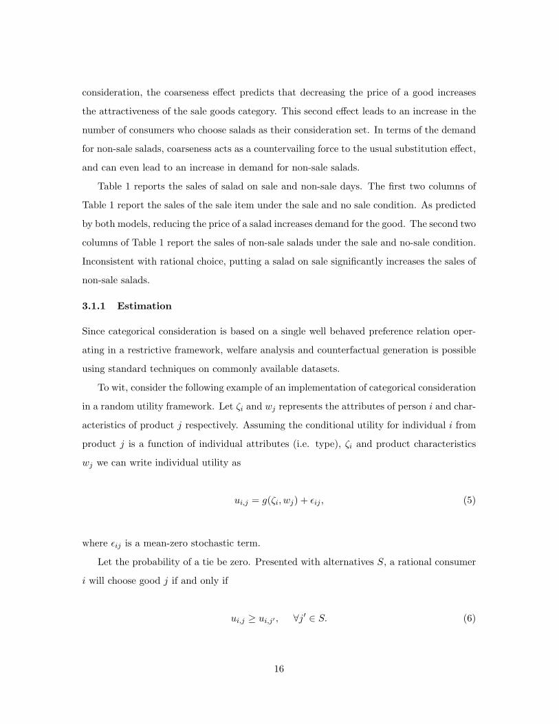
ui,j = g(ζi, wj) + εij , (5)

where εij is a mean-zero stochastic term.

Let the probability of a tie be zero. Presented with alternatives S, a rational consumer

i will choose good j if and only if

ui,j ≥ ui,j′ , ∀j′ ∈ S. (6)

16

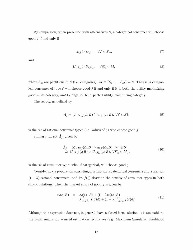
By comparison, when presented with alternatives S, a categorical consumer will choose

good j if and only if

ui,j ≥ ui,j′ , ∀j′ ∈ Sm, (7)

and

Ui,Sm ≥ Ui,S′m

, ∀S′m ∈ M, (8)

where Sm are partitions of S (i.e. categories): M ≡ {S1, . . . , SM} = S. That is, a categor-

ical consumer of type ζ will choose good j if and only if it is both the utility maximizing

good in its category, and belongs to the expected utility maximizing category.

The set Aj , as defined by

Aj = {ζ : ui,j(ζi;B) ≥ ui,j′(ζi;B), ∀j′ ∈ S}, (9)

is the set of rational consumer types (i.e. values of ζ) who choose good j.

Similary the set Aj , given by

Aj = {ζ : ui,j(ζi;B) ≥ ui,j′(ζi;B), ∀j′ ∈ S& Ui,Sm(ζi;B) ≥ Ui,S′

m(ζi;B), ∀S′

m ∈ M}. (10)

is the set of consumer types who, if categorical, will choose good j.

Consider now a population consisting of a fraction λ categorical consumers and a fraction

(1 − λ) rational consumers, and let f(ζ) describe the density of consumer types in both

sub-populations. Then the market share of good j is given by

sj(x;B) = λscj(x;B) + (1− λ)sr

j(x;B)= λ

∫ζ∈Aj

f(ζ)dζ + (1− λ)∫ζ∈Aj

f(ζ)dζ. (11)

Although this expression does not, in general, have a closed form solution, it is amenable to

the usual simulation assisted estimation techniques (e.g. Maximum Simulated Likelihood

17

(SML), Method of Simulated Moments (MSM), or Method of Simulated Score (MSS)).16 As

such the only additional burden categorical consideration places on estimation is knowing

the frame ` used by categorical consumers in a market (i.e. how the consumer partitions a

set of goods).

Since the rational model corresponds a restricted version of the mixed model (i.e. λ = 0),

one can use a simulated likelihood ratio test to directly test the full rationality restriction.

Consider then the following implementation of a very simple linear random-coefficient

model when consumers partition goods into salads and non-salads. Consumer utility from

purchasing good j can then be written as

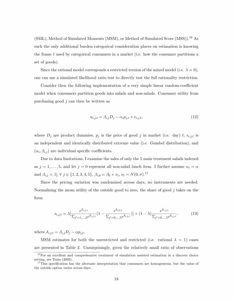
ui,j,t = βi,jDj − αipj,t + εi,j,t, (12)

where Dj are product dummies, pj is the price of good j in market (i.e. day) t, εi,j,t is

an independent and identically distributed extreme value (i.e. Gumbel distribution), and

(αi, βi,j) are individual specific coefficients.

Due to data limitations, I examine the sales of only the 5 main treatment salads indexed

as j = 1, . . . , 5, and let j = 0 represent all non-salad lunch item. I further assume αi = α

and βi,j = βj ∀ j ∈ {1, 2, 3, 4, 5}, βi,0 = β0 + νi, νi ∼ N(0, σ).17

Since the pricing variation was randomized across days, no instruments are needed.

Normalizing the mean utility of the outside good to zero, the share of good j takes on the

form

si,j,t = λ[eδi,j,t

Σj′=1,...,5eδi,j,t(1− eδi,0,t

Σj′=0,...,5eδi,j,t)] + (1− λ)

eδi,j,t

Σj′=0,...,5eδi,j,t. (13)

where δi,j,t = βi,jDj − αpj,t.

MSM estimates for both the unrestricted and restricted (i.e. rational λ = 1) cases

are presented in Table 2. Unsurprisingly, given the relatively small ratio of observations16For an excellent and comprehensive treatment of simulation assisted estimation in a discrete choice

setting, see Train (2003).17This specification has the alternate interpretation that consumers are homogeneous, but the value of

the outside option varies across days.

18

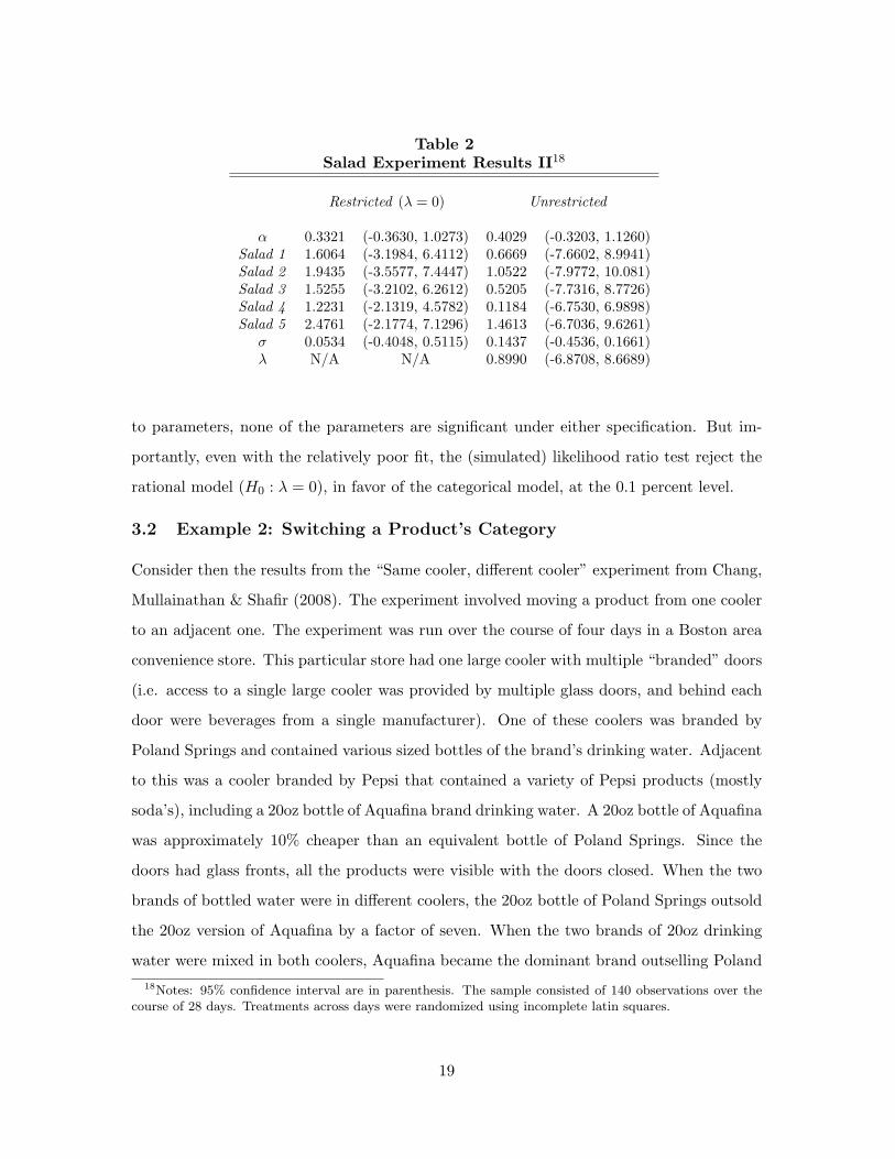
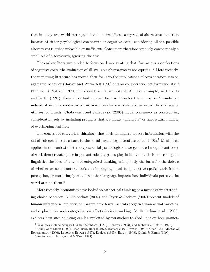
Table 2Salad Experiment Results II18

Restricted (λ = 0) Unrestricted

α 0.3321 (-0.3630, 1.0273) 0.4029 (-0.3203, 1.1260)Salad 1 1.6064 (-3.1984, 6.4112) 0.6669 (-7.6602, 8.9941)Salad 2 1.9435 (-3.5577, 7.4447) 1.0522 (-7.9772, 10.081)Salad 3 1.5255 (-3.2102, 6.2612) 0.5205 (-7.7316, 8.7726)Salad 4 1.2231 (-2.1319, 4.5782) 0.1184 (-6.7530, 6.9898)Salad 5 2.4761 (-2.1774, 7.1296) 1.4613 (-6.7036, 9.6261)

σ 0.0534 (-0.4048, 0.5115) 0.1437 (-0.4536, 0.1661)λ N/A N/A 0.8990 (-6.8708, 8.6689)

to parameters, none of the parameters are significant under either specification. But im-

portantly, even with the relatively poor fit, the (simulated) likelihood ratio test reject the

rational model (H0 : λ = 0), in favor of the categorical model, at the 0.1 percent level.

3.2 Example 2: Switching a Product’s Category

Consider then the results from the “Same cooler, different cooler” experiment from Chang,

Mullainathan & Shafir (2008). The experiment involved moving a product from one cooler

to an adjacent one. The experiment was run over the course of four days in a Boston area

convenience store. This particular store had one large cooler with multiple “branded” doors

(i.e. access to a single large cooler was provided by multiple glass doors, and behind each

door were beverages from a single manufacturer). One of these coolers was branded by

Poland Springs and contained various sized bottles of the brand’s drinking water. Adjacent

to this was a cooler branded by Pepsi that contained a variety of Pepsi products (mostly

soda’s), including a 20oz bottle of Aquafina brand drinking water. A 20oz bottle of Aquafina

was approximately 10% cheaper than an equivalent bottle of Poland Springs. Since the

doors had glass fronts, all the products were visible with the doors closed. When the two

brands of bottled water were in different coolers, the 20oz bottle of Poland Springs outsold

the 20oz version of Aquafina by a factor of seven. When the two brands of 20oz drinking

water were mixed in both coolers, Aquafina became the dominant brand outselling Poland18Notes: 95% confidence interval are in parenthesis. The sample consisted of 140 observations over the

course of 28 days. Treatments across days were randomized using incomplete latin squares.

19

springs by almost a factor of two.19

Though these results are clearly difficult to reconcile with neoclassical demand, they are

fully consistent with categorical consideration. Specifically, when the two brands of bottled

water were in separate coolers, even though the two different brands of 20oz drinking water

are close substitutes, they need not display much cross-price elasticity. But when they were

in the same cooler (category), we’d expect a high level of cross-price elasticity. Insofar as

they are equivalent goods (i.e. conditional on price, they provide equivalent utility), we

would expect to see a large shift from Poland Springs to the slightly cheaper Aquafina.

It is important to note that the cooler location does not provide a categorical considerer

with any objectively useful information unavailable to rational consumers. That is, just

like a neoclassical consumer, a categorical considerer does not believe cooler location in

and of itself impacts the utility of a good (i.e. it is an informationless label). Rather it

impacts choice because the label “cooler” is used by a categorical considerer as a type of

organizational or bookkeeping device to determine product categories.

3.3 Example 3: Changing Frames

If a product attribute x does not impact utility (i.e. dudx = 0), I refer to it as a label. Since

labels, by definition, have no impact on utility, demand is unaffected by non-informational

labels under standard rational choice.

A second common variant of informationless labeling is what I refer to as redundant

labels, or those labels that correspond to an already observable product attribute. Examples

include the packaging of some sugar based candies that declare their contents as having

“low fat”20, car dealerships writing descriptive phrases like “fuel efficient”21, or EnergyStar

certification for appliances.22

19This factor of 2 is likely a lower bound since during one of the mixed periods, demand for Aquafina wasso high as to generate a stockout during one of the treatment days.

20As is currently the case for Twizzlers, York Peppermint Pattie, Jolly Ranchers, Good & Plenty, andHershey’s Chocolate Syrup.

21FTC regulation requires that all new and used cars sold in the US have prominent “window stickers”(a.k.a. a Monroney) that include numerical EPA fuel economy estimates, labeling a car as “fuel efficient”is redundant.

22U.S. Federal law (administered by the U.S. Department of Energy) requires appliances have a prominentEnergyGuide Label that provides estimated numeric operating costs/electricity use in comparison to similarmodels. EnergyStar is a more recent program jointly administered by the U.S. Department of Energy andthe U.S. Environmental Protection Agency that allows firms to place an “Energy Star logo” on an appliance

20

It is important to note that conditional on a frame `, choice will vary if and only if the

actual underlying distribution of utility changes. As in the rational model, conditional on

`, branding, non-informational labeling, and other marketing devices that do not directly

impact product utility will not affect decision making.

Similar to the rational model, when product partitions are fixed, categorical demand

is unaffected by non-informational labels. But to the extent that labels can affect the

categories a consumer uses, labels can generate a change in product demand. One prediction

of categorical consideration is that non-informational labels can impact consumer choice by

changing how individuals partitions a set of goods.

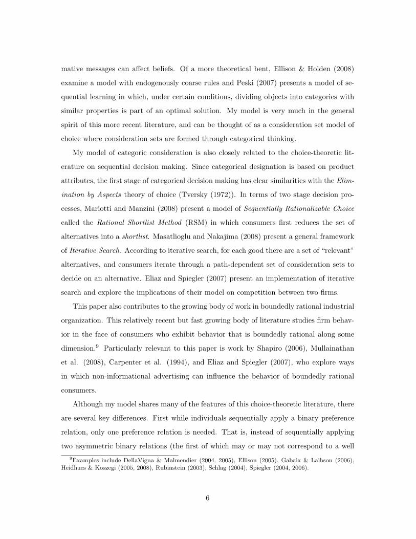
An example of this type of behavior is found in Poilane (2007). Poilane ran a series

of field experiments in three upscale bakeries. In the experiments she alternated between

three different labeling conditions for a set of 12 jams. In one condition jams were presented

without labels. In the second treatment jams were organized into three groups of four,

with each group getting a descriptive category name (citrus, berry, nutty). In the final

treatment, the descriptive labels were replaced with randomly assigned names (“the baker”,

“the pastry chef”, “the apprentice”). Table 3 presents the average weekly jam sales under

each treatment condition.

Although product sales are not affected by the use of random category names, the

use of descriptive category names significantly decreased total sales. For comparison, the

magnitude of this decrease was on par with reducing the set of available jams by half.24

The observed behavior is clearly inconsistent with the predictions of rational model under

which the use of non-informative or redundant labels should not affect demand. In addition,

insofar as redundant labels decrease search costs, this result is inconsistent with rational

search cost models which would predict weakly increased demand under the descriptive

label treatment.25

The observed behavior is however consistent with categorical consideration. Specifically

if the appliance meets a certain level of efficiency compared to similar models based on the EnergyGuideratings.

23Notes: Standard errors are in parenthesis. The regression store fixed effects. Treatments were random-ized according to an incomplete latin square design.

24See Poilane (2007).25In point of fact the original goal of the experiment was to see if the use of descriptive category labels

could increase sales by decreasing consumer search costs.

21

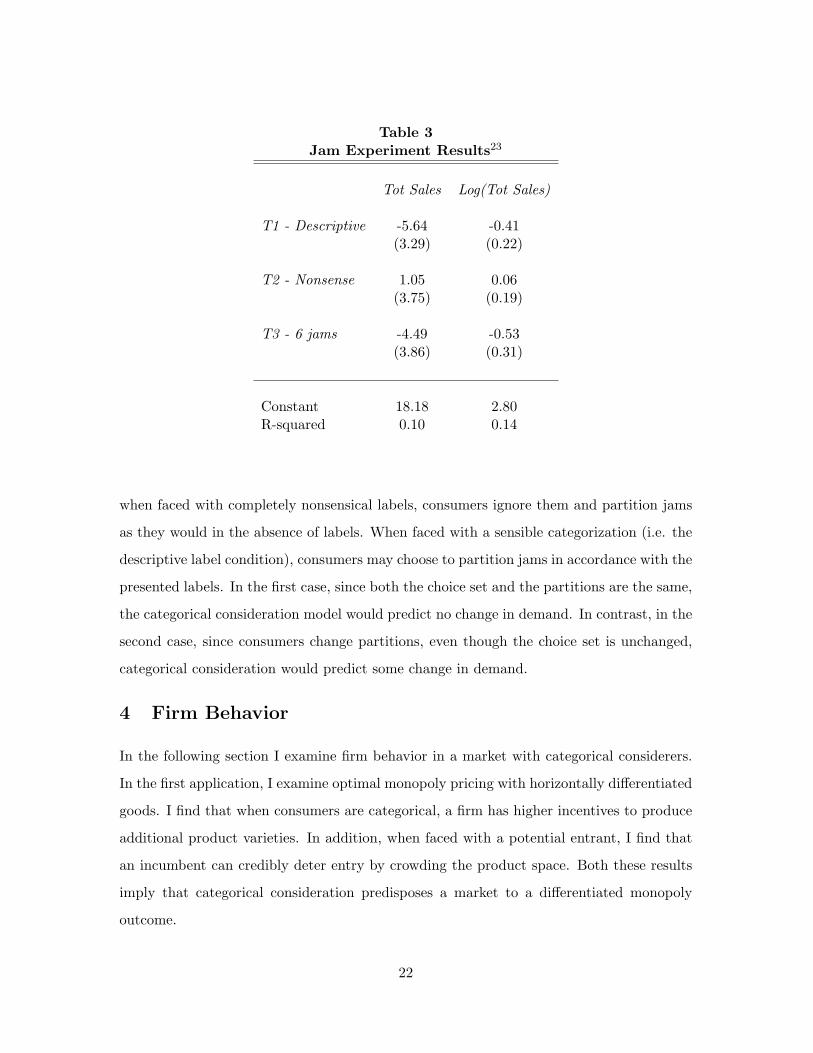
Table 3Jam Experiment Results23

Tot Sales Log(Tot Sales)

T1 - Descriptive -5.64 -0.41(3.29) (0.22)

T2 - Nonsense 1.05 0.06(3.75) (0.19)

T3 - 6 jams -4.49 -0.53(3.86) (0.31)

Constant 18.18 2.80R-squared 0.10 0.14

when faced with completely nonsensical labels, consumers ignore them and partition jams

as they would in the absence of labels. When faced with a sensible categorization (i.e. the

descriptive label condition), consumers may choose to partition jams in accordance with the

presented labels. In the first case, since both the choice set and the partitions are the same,

the categorical consideration model would predict no change in demand. In contrast, in the

second case, since consumers change partitions, even though the choice set is unchanged,

categorical consideration would predict some change in demand.

4 Firm Behavior

In the following section I examine firm behavior in a market with categorical considerers.

In the first application, I examine optimal monopoly pricing with horizontally differentiated

goods. I find that when consumers are categorical, a firm has higher incentives to produce

additional product varieties. In addition, when faced with a potential entrant, I find that

an incumbent can credibly deter entry by crowding the product space. Both these results

imply that categorical consideration predisposes a market to a differentiated monopoly

outcome.

22

I next examine competition between branded and generic goods in a horizontally differ-

entiated market. Specifically I examine optimal pricing for a single product regional brand

competing with a multi-product national brand. The main result is that when consumers

are categorical, there can exist a wedge between the price of two identical items. That is,

when consumers are boundedly rational, the insurance effect of having a larger product line

allows the national brand to charge a higher price than a physically identical generic.

In the final application I examine how, in the presence of categorical consumers, a firm

can increase differentiation through branding. Specifically when consumers think coarsely

about brands, a firm’s strategy of selling their products under multiple brands (even if

brand is an uninformative label) may be optimal.

4.1 Product Proliferation

Consider the following variation of the basic model in Section 3 with horizontal product

differentiation. There is a single firm that sells horizontally differentiated goods L and R

at prices pL and pR. The firm can produce either good at constant marginal costs cj and

fixed cost F .

There is a measure one of homogeneous consumers. For consumer i the stochastic

element ηi can take on values {0, 1} where the probability that η = 1 is given by σ:

Pr(ηi = 1) = σ. The interpretation here is that consumers have a preference for one of the

two varieties, but initially have only a (correct) belief as to which good that will be. In

addition to goods {L,R}, there is a third option M which provides consumers with utility

v′ < v. Consumer wish to purchase at most one of the products and receives zero utility

from purchasing nothing. Consumer utility from product j ∈ {L,R,M} is then given by

ui(j, pj ; ηi) ={ v − t(1− ηi)− pL if j = L

v − tηi − pR if j = Rv′ if j = j = M

(14)

A fraction λ of all consumers are categorical considerers who partition the products

{L,R} separately from M : if faced with the choice set S = {L,R,M}, a categorical

considerer will partition the set into the categories S1 = {L,R} and S0 = {M}. For

example consider an individual choosing between two types of soup or a salad for lunch or

23

deciding whether to go out to one of two currently playing action movies or staying home

to watch a favorite TV show.

For simplicity consider the case where t > v so that for non-negative prices there is at

most one good from the set {L,R} that provides the consumer with non-negative surplus.

Then for pj ≤ v ∀j, categorical consumer’s expected utility for a set of goods Sm is

u(Sm, pj ;σ) =

{ σ[v − pL] + (1− σ)[v − pR] if Sm = {L,R}σ[v − pL] if Sm = {L}

(1− σ)[v − pR] if Sm = {R}v′ if Sm = {M}

(15)

First assume that all consumers are rational (λ = 0). Then conditional on producing

either good, the firm will price them both at price pj = v−v′. The firm chooses to produce

a good if the profits exceed the fixed cost F . That is, it will produce good L if σ(v−v′) > F

and good R if (1− σ)(v − v′) > F .

Now assume that all consumers are categorical (λ = 1). According to equation 15, the

maximum price the firm can charge for a good is dependent on whether or not it carries the

other good. For example conditional on producing only the single good L (R), the highest

price the firm could charge is pL(R) = v − v′

σ .

If instead the firm produces both goods, then an individual will consider the set of goods

S1 = {L,R} if σ[v − pL] + (1− σ)[v − pR] ≥ v′. And conditional on considering set S1, the

individual will purchase a good if MAX{v − t(1− ηi)− pL, v − tηi − pR} ≥ 0.

This simple example captures the two main features of categorical consideration: coarse

thinking and limited consideration. Coarse thinking materializes because consumers do not

decide to evaluate goods on a product by product basis, but instead decide whether or

not to evaluate the firm’s product line as a whole. Limited consideration comes from the

fact that after choosing a preferred category, consumers purchase the best good in the

bundle conditional on that good providing positive surplus. That is, consumers do not take

into account the expected value for other available, but not evaluated goods (i.e. goods

outside their consideration set), but act as if the considered goods constituted the full set

of available goods.

24

4.1.1 Monopoly Pricing

To see the impact of categorical consideration on firm pricing behavior, let us first consider

the following basic game. In step one, a single firm decides what products (if any) to sell

and at what prices conditional on knowing both the distribution of types σ and the share

of categorical consumers λ. In step two, individuals see prices and choose which goods to

consider.26 Then in step three, individuals evaluate the considered goods (i.e. learn ηi) and

decide whether or not to purchase one of the considered goods.

Proposition 1 Let M and M ′ be two markets with a fraction λ and λ′ of behavioral con-

sumers where λ 6= λ′. For any set of parameters (v, v′, t, σ, F ), conditional on entry, the

number of product varieties is weakly greater in the market with a larger fraction of cate-

gorical considerers.

Proof: See appendix. �

The intuition for this result is quite simple: when consumers are categorical considerers,

goods have an option value. That is a categorical consumer will purchase a good from the

firm only if they first decide to seriously consider the firm’s products, and by having more

varieties the firm increases the expected value of its goods to an individual.

The key implication of this proposition is that conditional on entry, a monopolist’s

product variety will increase in the share of boundedly rational consumers. In markets (or

product spaces) where a larger share of consumers act categorical, we would expect firms

to produce a larger number of product varieties than predicted in a fully rational model.

Note, though, that because firms need to produce more varieties for categorical than

rational consumers, effective entry costs are higher when consumers are categorical. We will

explore the implications of this result in more detail in our analysis of competitive market

settings, but the main intuition here is that the presence of categorical consumers biases a

market toward multi-product monopoly.

In costly rational search models like that found in Lal & Matutes (1994), products in a

store are physically linked together by travel costs. In a similar way, products in a category

are mentally linked together by limited consideration. Then in the same way that in a costly26Fully rational consumers consider all available goods.

25

search model firms need to get customers into their store, under categorical consideration

firms need to get consumers to mentally consider their goods. Though these two results are

mathematically similar, they are quite different in their application. Specifically categorical

consideration, unlike rational search models, describes consumer decision making in cases

without a clear physical cost linking sets of goods (e.g. travel cost to different retail stores).

Instead it applies to any set of goods that consumers partition into mental categories.

4.2 Entry Deterrence

One implication of Proposition 1 is that the presence of categorical consumers biases a

monopolist toward product proliferation. But as we shall see, the threat of entry creates

an additional incentive for a monopolist to produce more varieties as a credible means of

entry deterrence.

A long standing argument holds that incumbent firms may be able to deter entry by

pre-emptive investment in new goods. For example Schmalensee (1978) argues that incum-

bent firms use excess product proliferation to deter entry by leaving no niche for potential

entrants. The intuition behind spatial preemption can be seen in the following example.

Imagine that A and B are the only two possible variants of a good, and that these goods

are produced at constant marginal cost after a one time set-up cost. Competition in the

market is in prices. The incumbent firm can then preclude entry into the product market

by spanning the space (i.e. producing both A and B). Then since post-entry price compe-

tition would drive down the price of a newly introduce good to marginal cost, the entrant

will make zero profit and will never recover the fixed set-up cost.

More recent work though has brought the theoretical foundations of such spatial pre-

emption into doubt. For example, Judd (1985) shows that as long as incumbents are allowed

to exit in response to entry by another firm, spatial preemption is not a credible deterrence

to entry. The basic insight of Judd (1985) was to point out that previous models of spatial

preemption precluded (limited) exit by the incumbent firm. Absent prohibitively high exit

costs, the incumbent has a unique ex-post incentive to stop producing certain product va-

rieties. Specifically, assume that the incumbent produces good A and B while the entrant

produces only good A. Then since A and B are substitutes, the intense price competition

26

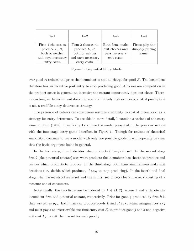
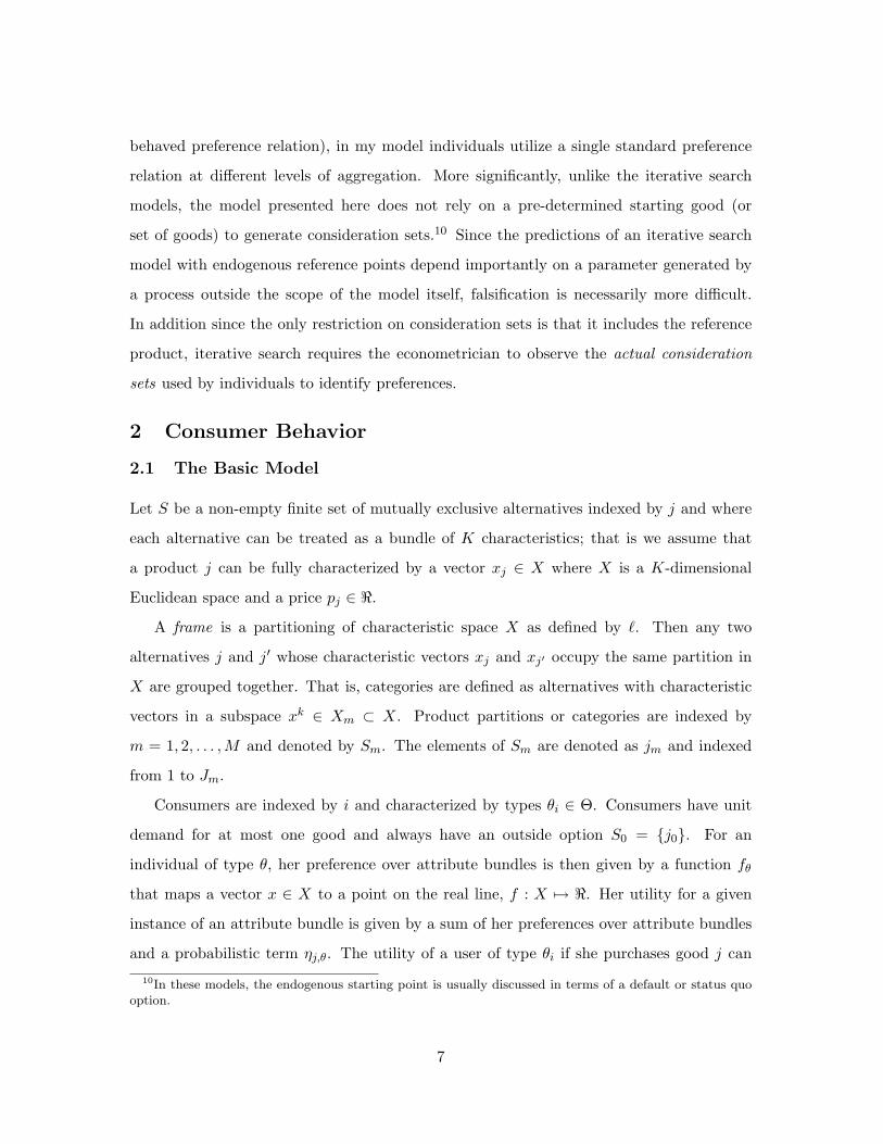
t=1 t=2 t=3 t=4

Firm 1 chooses to Firm 2 chooses to Both firms make Firms play theproduce L, R, produce L, R, exit choices and duopoly pricingboth or neither both or neither pays necessary game.

and pays necessary and pays necessary exit costs.entry costs. entry costs.

Figure 1: Sequential Entry Model

over good A reduces the price the incumbent is able to charge for good B. The incumbent

therefore has an incentive post entry to stop producing good A to weaken competition in

the product space in general; an incentive the entrant importantly does not share. There-

fore as long as the incumbent does not face prohibitively high exit costs, spatial preemption

is not a credible entry deterrence strategy.

The presence of categorical considerers restores credibility to spatial preemption as a

strategy for entry deterrence. To see this in more detail, I examine a variant of the entry

game in Judd (1985). Specifically I combine the model presented in the previous section

with the four stage entry game described in Figure 1. Though for reasons of rhetorical

simplicity I continue to use a model with only two possible goods, it will hopefully be clear

that the basic argument holds in general.

In the first stage, firm 1 decides what products (if any) to sell. In the second stage

firm 2 (the potential entrant) sees what products the incumbent has chosen to produce and

decides which products to produce. In the third stage both firms simultaneous make exit

decisions (i.e. decide which products, if any, to stop producing). In the fourth and final

stage, the market structure is set and the firm(s) set price(s) for a market consisting of a

measure one of consumers.

Notationally, the two firms are be indexed by k ∈ {1, 2}, where 1 and 2 denote the

incumbent firm and potential entrant, respectively. Price for good j produced by firm k is

then written as pj,k. Each firm can produce goods L and R at constant marginal costs cj

and must pay a an irretrievable one-time entry cost Fe to produce good j and a non-negative

exit cost Fx to exit the market for each good j.

27

As in the previous section, there are a measure one of homogeneous consumers with

unit demand for at most one good. Utility from product j ∈ {L,R, j0} is

ui(j, pj ; ξi) ={ v + t(1− ξi)− pL if j = L

v + tξi − pR if j = Rv′ if j = j0

(16)

where ξi ∈ {0, 1}, Pr(ξi = 1) = σ, and j0 is the outside option (e.g. non-purchase). WLOG

I set v′ = 0 cj = 0 ∀j. I further assume t < V so that the goods L and R are similar enough

to be viable substitutes.

Proposition 2 Let all consumers be fully rational. If there exists a pure strategy equilib-

rium that supports a differentiated duopoly that is profitable net of fixed cost, then for low

enough exit costs (Fx < F x) the incumbent firm cannot credibly prevent entry by crowding

the product space.

Proof: See appendix. �

The intuition behind the proof of the proposition is the same as in the more general case

presented in Judd (1985). Specifically, if firm 2 enters the market for just one of the two

goods, for low enough exit costs, the profit maximizing strategy for the incumbent post-

entry is to accommodate entry, and exit the contested market. Because the competition in

the overlapping good adversely affects the profit the firm earns on the other good, multi-

product incumbents have an ex-post incentive to accommodate entry and thereby weaken

competition in the market as a whole. Importantly firm 2 faces no ex-post incentive to exit

so will never exit a market for any non-negative exit cost.

Proposition 3 Let all consumers be categorical considerers. The incumbent firm can suc-

cessfully (credibly) preclude entry by crowding the the product space.

Proof: See appendix. �

This result is due to the fact that in a market of categorical considerers, the incumbent

firm does not face an ex-post incentive to (partially) exit the market. For concreteness,

consider the possible competitive stage 4 outcomes where σ = 12 (Figure 1).

28

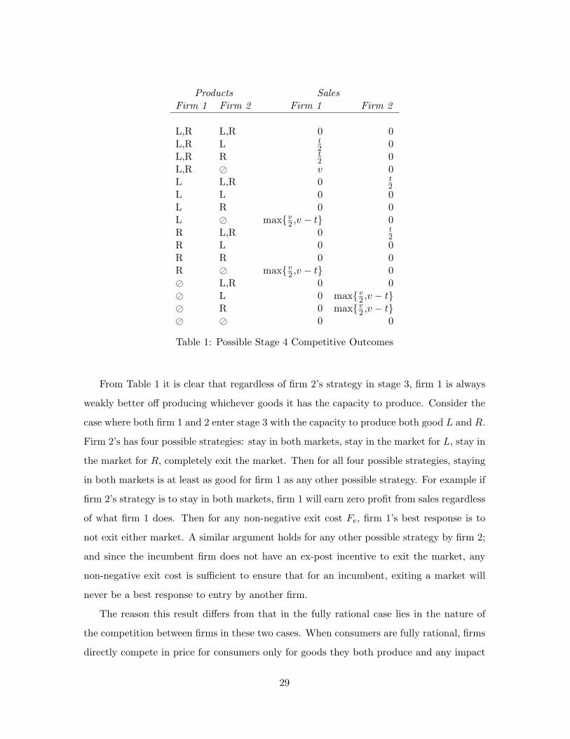
Products SalesFirm 1 Firm 2 Firm 1 Firm 2

L,R L,R 0 0L,R L t

2 0L,R R t

2 0L,R � v 0L L,R 0 t

2L L 0 0L R 0 0L � max{v

2 ,v − t} 0R L,R 0 t

2R L 0 0R R 0 0R � max{v

2 ,v − t} 0� L,R 0 0� L 0 max{v

2 ,v − t}� R 0 max{v

2 ,v − t}� � 0 0

Table 1: Possible Stage 4 Competitive Outcomes

From Table 1 it is clear that regardless of firm 2’s strategy in stage 3, firm 1 is always

weakly better off producing whichever goods it has the capacity to produce. Consider the

case where both firm 1 and 2 enter stage 3 with the capacity to produce both good L and R.

Firm 2’s has four possible strategies: stay in both markets, stay in the market for L, stay in

the market for R, completely exit the market. Then for all four possible strategies, staying

in both markets is at least as good for firm 1 as any other possible strategy. For example if

firm 2’s strategy is to stay in both markets, firm 1 will earn zero profit from sales regardless

of what firm 1 does. Then for any non-negative exit cost Fe, firm 1’s best response is to

not exit either market. A similar argument holds for any other possible strategy by firm 2;

and since the incumbent firm does not have an ex-post incentive to exit the market, any

non-negative exit cost is sufficient to ensure that for an incumbent, exiting a market will

never be a best response to entry by another firm.

The reason this result differs from that in the fully rational case lies in the nature of

the competition between firms in these two cases. When consumers are fully rational, firms

directly compete in price for consumers only for goods they both produce and any impact

29

on other goods are due to spillover effects. If instead consumers are categorical considerers,

firms compete not product by product, but rather product-line by product-line. As such

exiting from a highly contested market does not decrease the competition between the firms

in other markets. But since having more products increases the attractiveness of a product

line, it does have the effect of weakening the exiting firm’s overall ability to compete with

another firm.

4.3 Brand Name Premium

A consistently observed but somewhat striking empirical fact is the significant price pre-

mium branded products have over physically identical generic goods. Although the standard

argument that branded goods are of higher quality than generics is surely correct in many

instances, in many others it seems quite implausible. For example even though Chlorox

bleach is chemically and Reynolds Aluminum Foil is physically identical to their generic

equivalents, the branded goods still sell at significant price premiums.27

Another particularly striking example is the existence of “branded generics.” Though

studied most often in the context of entry deterrence, one somewhat surprising fact is that

pharmaceutical firms occasionally sell generic versions of their good.28 These so called

“branded generics” are physically identical to the branded good, manufactured often in the

same plant in the same production lines, but sold under a different trade name.29 Even in

the presence of branded generics, the branded drug not only sells at a significant premium

compared to the branded generic, but also maintains a significant market share.

Consider the model of horizontal consumer taste differentiation from the previous section

where thee market contains a heterogeneous mix of consumer types. As before there are

two feasible horizontally differentiated varieties of a good denoted by {L,R}, and consumer

utility from purchasing a good is given by

ui(j, pj ; ξi) ={ v + t(1− ξi)− pL if j = L

v + tξi − pR if j = Rv′ if j = j0

(17)

27On 9/11/2008 the online grocery store Peapod sold Chlorox bleach and Reynolds Aluminum Foil at a30.0% and 43.0% higher than the available generic equilvalents.

28See for example Liang (1996), Ferrandiz (1999) and Kamien & Zang (1999).29Hollis (2003).

30

where j0 is the outside option. As before ξi ∈ {0, 1}, but now Pr(ξi = 1) = θi and

distribution of θi is characterized by a CDF F (θ).

A fraction λ of all consumers are categorical considerers who use product brand (i.e.

the manufacturing firm) to partition products. The remaining 1 − λ consumers are fully

rational (i.e. their consideration sets are the full set of available goods).

I model competition between a small regional brand and a large national brand as

follows. Notationally I refer to the national brand as firm A and the regional brand as firm

B: k ∈ {A,B}. The national brand can produce either varieties of the good SA = {L,R}

while the regional brand can only produce one variety SB = {L}. All goods are produced

at a constant marginal cost c which WLOG I set to zero.

Analogous to the small open economy assumption in Macroeconomics, I assume that

the national brand does not adjust its strategy in response to the regional brand. Though

the argument presented here holds as long as the national brand has monopoly power over

some fraction of the population, a detailed general analysis would be tedious and detract

from the basic point.

Assume then that the national brand sets prices pA ≡ pA,L = pA,R < v. Since firm B

produces only one good, for notational simplicity I will drop the j subscript and refer to

pB,L simply as pB.

Proposition 4 Let all consumers be fully rational (λ = 0). The regional brand’s profit

maximizing strategy is to price ε below the national brand’s price for the identical good LA.

Proof: Since LA and LB are undifferentiated (i.e. identical) goods, consumers will buy

from the firm that charges the lowest price. And since demand for LB is constant for any

price pB < pA, the regional brands best response is to just undercut firm A’s price on good

L. �

Proposition 5 The regional brand’s profit maximizing price p∗B,L is decreasing in the share

of categorical considerers: p∗B,L(λ′) ≤ p∗B,L(λ) ∀ λ′ > λ.

Proof: A consumer of type θ will consider the regional brand if U(SB, pB) ≥ U(SA, pA).

Therefore the marginal customer type that considers the regional brand is given by

31

v − pA = (1− θ)[v + t− pB] + θ[v − pB]v − pA + t = v − pB − (1− θ)t

=⇒ θ∗ = pA−pBt

(18)

For pB < pA, the demand faced, and profit earned, by the regional brand product is then

DB(pB|pA, λ) = (1− λ) + λF (θ∗) (19)

πB(pB|pA, λ) = [(1− λ) + λF (θ∗)]pB (20)

respectively. Taking the first order condition I find

∂π

∂pB= (1− λ) + λ

[F (θ∗)− pB

tf(θ∗)

]= 0, (21)

where f(·) is the pdf of the distribution of consumer types. Some simple algebraic manip-

ulation of the FOC leads to the condition

(1− 1

λ

)= F (θ∗)− pB

tf(θ∗). (22)

Note that the left hand side of equation 22 is increasing in λ: ∂∂λ

(1− 1

λ

)> 0. As such, to

prove that pA is decreasing in λ it is sufficient to show that the right hand side of equation

22 is decreasing in pA.

For a small change in pA the change in the right hand side of equation 22 is given by

∆∆pA

(F (θ∗)− pB

t f(θ∗))

= f(θ∗)∆pA − 1t

(f(θ∗)∆pA + O(p2

A))

= −(1 + 1t )f(θ∗)∆pA − 1

t O(p2A)

≈ −(1 + 1t )f(θ∗)∆pA.

(23)

As ∆pA → 0, we can ignore the higher order terms, and since the pdf f(·) is non-negative,

the expression is decreases in pA. �

32

This predicted pattern of behavior (i.e. brands with more extensive produce lines charge

higher prices) is one largely consistent with the observation that branded goods have both

more variety and higher prices than their generic equivalents. Returning to the previously

discussed cases of bleach and aluminum foil, we see that the national brands tend to not

only be priced higher, but have more varieties than their generic equivalents.30

4.4 Differentiation Through Brands

So far all our examples have focused on optimum firm behavior when product categories

were fixed (i.e. consumers partition goods by brand). The main result of the previous

examples have involved how firms can use genuine product differentiation to their advantage

when consumers are categorical. In this example, I show how a firm can use branding to

artificially create product differentiation.

Though a full discussion of this topic is beyond the scope of this paper, I briefly

discuss categorical consideration as a micro-foundation for product placement and non-

informational advertising.

Under categorical consideration, leading brands may have an incentive to keep their

products physically separated from competing goods if such physical placement induces

consumers to treat their brand as a separate category. As a specific example, consider the

previously discussed experiment involving bottled water. Given the large drop in Aquafina

sales when a less expensive, competing brand was mixed across coolers as opposed to being

located in separate but adjacent coolers, Poland Springs clearly has an incentive to pay

retailers to keep their products physically separate from bottles of Aquafina.

For example in 2006 First Marblehead, one of the dominant providers of private edu-

cation lending in the US, marketed their student loan products through several different

brands. Although each brand had its own unique identity, advertising campaign, etc. they

each offered the exact same loans. The idea behind this marketing strategy was to create

the illusion of product differentiation for a homogeneous financial instrument - that is, to

use product branding to differentiate money.

To fix the idea, consider the case of the auto manufacturer Toyota. Toyota is a brand30On 9/11/2008 the online grocery store Peapod sold 7 variants of Chlorox bleach compared to 2 variants

of the generic bleach and 4 versions Reynolds Aluminum Foil compared to 2 variants of generic foil.

33

best known as a high quality manufacturer of mid-range cars, but in the 1980s it wanted

to start competing in the high end market against brands like BMW and Mercedes Benz.

In the absence of categorical consideration, Toyota’s reputation for quality and reliability

in the mid-range cars would be an asset in competing in the high end market, as would

the ability to leverage the extensive network of Toyota dealerships and brand recognition.

Instead Toyota chose to create a new brand Lexus under which to market and sell their

new high end automobiles.

Consider a consumer deciding which brands to considers under two alternate scenarios.

In the first Toyota sells both mid-range and luxury models under one brand. In the second,

Toyota sells their mid-range and luxury cars as different brands. Assume that selection of

luxury Toyota models is identical in both scenarios and that an identical car purchased in

either scenario provides the same level of utility to the buyer (i.e. the different dealerships

do not provide significantly different levels of amenities, nor is there any intrinsic benefit

to the consumer from the brand itself).

For simplicity assume Toyota sells only only two vertically differentiated cars M and H

at prices pM and pH . In addition to Toyota let there be two other firms k = m,h where

firms 1 and 2 manufactures a mid-range and high-end cars respectively. These products

are denoted by M ′ and H ′ and sold at prices p′M and p′H . All firms can produce all goods

at constant marginal cost c.

Consumers differ along two dimensions: whether or not they value “luxury” α and a

horizontal taste parameter θ. Let there be a unit mass of consumers who do not value

luxury (α = 0) and a unit mass of consumers with do (α = 1). Consumer i who value

luxury derive utility Uvi = v from luxury cars, and zero utility from mid-range cars while

the opposite is true for consumers who do not value luxury. In addition the stochastic term

ηi ∈ {0, t} determines which firms car matches their personal tastes.

Consumers buy at most one car and receive zero utility from not making a purchase. A

fraction λ of all consumers are categorical and Pr(η = t) = 12 . The utility a consumer of

type (α, θ) will obtain from purchasing a good is then given by

34

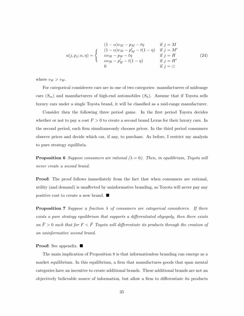
u(j, pj ;α, η) =

{ (1− α)vM − pM − tη if j = M(1− α)vM − p′M − t(1− η) if j = M ′

αvH − pH − tη if j = HαvH − p′H − t(1− η) if j = H ′

0 if j = �

(24)

where vH > vH .

For categorical considerers cars are in one of two categories: manufacturers of midrange

cars (Sm) and manufacturers of high-end automobiles (Sh). Assume that if Toyota sells

luxury cars under a single Toyota brand, it will be classified as a mid-range manufacturer.

Consider then the following three period game. In the first period Toyota decides

whether or not to pay a cost F > 0 to create a second brand Lexus for their luxury cars. In

the second period, each firm simultaneously chooses prices. In the third period consumers

observe prices and decide which car, if any, to purchase. As before, I restrict my analysis

to pure strategy equilibria.

Proposition 6 Suppose consumers are rational (λ = 0). Then, in equilibrium, Toyota will

never create a second brand.

Proof: The proof follows immediately from the fact that when consumers are rational,

utility (and demand) is unaffected by uninformative branding, so Toyota will never pay any

positive cost to create a new brand. �

Proposition 7 Suppose a fraction λ of consumers are categorical considerers. If there

exists a pure strategy equilibrium that supports a differentiated oligopoly, then there exists

an F > 0 such that for F < F Toyota will differentiate its products through the creation of

an uninformative second brand.

Proof: See appendix. �

The main implication of Proposition 8 is that informationless branding can emerge as a

market equilibrium. In this equilibrium, a firm that manufactures goods that span mental

categories have an incentive to create additional brands. These additional brands are not an

objectively believable source of information, but allow a firm to differentiate its products

35

in the minds of categorical considerers. Put another way, when consumers use product

brand as a means to reduce a set of alternatives to a more manageable consideration set,

dividing a product line into multiple brands allows a firm to more effectively target specific

consumers.

This result is in direct opposition to the standard model in which a larger product-line

must be (weakly) more attractive to consumers - i.e. more is better. For example if there

were a fixed cost to visiting a dealership, conditional on prices, a dealership has a built in

advantage over another dealership whose product line is a strict subset of its own. But when

consumers are categorical, they do not compare goods item by item, but instead brand by

brand. This idea that firms compete with each other not in terms of equivalent products,

but instead in terms of brands or entire product lines, is consistent with discussions the

marketing literature.31

5 Conclusion

This paper presents a simple model of boundedly rational decision making that explains

both a diverse set of non-rational consumer behavior, but also seemingly anomalous mar-

keting strategies by firms. Specifically when product categories are fixed I find that when

consumers are categorical, markets tend toward multi-product monopoly in comparison to

the rational baseline. In addition the option value of goods when consumers are boundedly

rational leads to market equilibriums in which a firms with larger product lines can charge

higher prices for physically identical goods. If instead firms can manipulate consumer cat-

egories, I show how firms can differentiate their products through brand creation.

In the model presented here individuals have well defined preferences, but exhibit two

biases compared to fully rational consumers. First because of limited consideration, indi-

viduals choose the utility maximizing good from a limited subset of alternatives. Second

since individual preference are applied coarsely to categories, the probability that an al-

ternative is considered is affected by other “irrelevant” products. The model includes the

standard rational model as a special case.

Perhaps the most common critique of behavioral models is that because they can ac-31See for example Katz (1984) or Brander and Eaton (1984).

36

commodate most any choice behavior, they are not actually informative. One advantage of

categorical consideration, relative to most behavioral models, is that it provides a restrictive

framework for decision making that still manages to explain a range of interesting behavioral

anomalies. Because decision making is based on a single well behaved preference relation,

many of the insights, intuitions, and empirical methods based on the standard model either

apply directly to, or have simple analogues in, categorical consideration. Conditional on

categories, the fact that consumers have a single well behaved set of preference means that

those preferences are identifiable from choice data. Then insofar as a consumer’s choice of

categories is amenable to economic intuition (or experimental validation), welfare analysis

and counterfactual testing is possible using commonly available datasets.

37

References

Bayus, Barry and William Putsis, “Product Proliferation: An Empirical Analysis of Prod-uct Line Determinants and Market Outcomes,” Marketing Science, 18(2) (1999), 137-153.

Brander, James A. and Jonathan Eaton, “Product Line Rivalry,” The American EconomicReview, 74(3) (1984), 323-334.

Carpenter, Gregory and Rashi Glazer, and Kent Nakamoto, “Meaningful Brands fromMeaningless Differntiation: The Dependence on Irrelevant Attributes,” Journal ofMarketing Research, 31 (1994), 339-350.

Chakravarti, Amitav and Chris Jaiszewski, “The Influence of Macro-Level Motives on Con-sideration Set Composition in Novel Purchase Situations,” Journal of Consumer Re-search, 30 (2003), 244-258.

Chang, Tom, Sendhil Mullainathan and Eldar Shafir, “Experiments in Choice,” Mimeo,MIT, (2008).

DellaVigna, S. and U. Malmendier, “Contract Design and Self-Control: Theory and Evi-dence,” Quarterly Journal of Economics, 119 (2004), 353-402.

DellaVigna, S. and U. Malmendier, “Paying Not to Go to the Gym,” American EconomicReview, 96 (2006), 694-659.

Eliaz, Kfir and Ran Spiegler, “Consideration Sets and Competitive Marketing,” Mimeo,(2007).

Eliaz, Kfir and Ran Spiegler, “Contracting with Diversely Nave Agents,” Review of Eco-nomic Studies, 73 (2006), 689-714.

Ellison, Glenn, “A Model of Add-On Pricing,” Quarterly Journal of Economics, 120 (2005),585-638.

Ellison, Glenn, “Bounded Rationality in Industrial Organization,” in Advances in Eco-nomics and Econometrics: Theory and Applications, Ninth World Congress, VolumeII, ed. by R. Blundell, W. Newey, and T. Persson. Cambridge University Press,Cambridge (2006).

Ellison, Glenn and Richard Holden, “A Theory of Rule Development,” Mimeo, MIT (2008).

Ferrandiz, J. M., “The Impact of Generic Goods in the Pharmaceutical Industry,” HealthEconomics, 8(7) (1999), 599-612.

Fryer, Roland and Mark Jackson, “A Categorical Model of Cognition and Biased Decision-Making,” Contributions in Theoretical Economics, B.E. Press, Forthcoming (2008).

Gabaix, Xavier and David Laibson, “Shrouded Attributes, Consumer Myopia, and Infor-mational Suppression in Competitive Markets,” Quarterly Journal of Economics, 121(2006), 505-540.

38

Hauser, John and Birger Wernerfelt, “An Evaluation Cost Model of Consideration Sets,”Journal of Consumer Research, 16 (1990), 383-408.

Hayward, W. G. and M. J. Tarr, “Spatial language and spatial representation,” Cognition,55 (1995), 39-84.

Hayward, W. G. and M. J. Tarr, “Testing conditions for viewpoint invariance in objectrecognition,” Journal of Experimental Psychology: Human Perception and Perfor-mance, 23 (1997), 1511-1521.

Heidhues, Paul and Botond Koszegi, “Competition and Price Variation when Consumersare Loss Averse,” American Economic Review, (2008a), 98(4), 1245-1268.

Heidhues, Paul and Botond Koszegi, “Exploiting Naivete about Self-Control in the CreditMarket,” Mimeo, (2008b).

Hollis, Aidan, “The Anti-Competitive Effects of Brand-Controlled ‘Pseudo-Generics’ in theCanadian Pharmaceutical Market,” Canadian Public Policy, 29(1) (2003), 21-32.

Iyengar, S and M. Lepper, “When Choice is Demotivating: Can One Desire Too Much ofa Good Thing?,” Journal of Personality and Social Psychology, 79 (2000), 995-1006.

Judd, Kenneth L., “Credible Spatial Preemption,” Rand Journal of Economics, 16(2),(1985), 153-166.

Kamien, M. I., and I. Zang,“Virtual Patent Extension by Cannibalization,” Southern Eco-nomic Journal, 66(1), (1999), 117-131.

Kuksov, Dmitri and J. Miguel Villas-Boas, “When More Alternatives Lead to Less Choice,”Mimeo, (2005).

Lal, R., and C. Matutes. ”Retail Pricing and Advertising Strategies.” Journal of Business,67, (1994), 345-370.

Liang, B.“The Anticompetitive Nature of Brand-Name Firm Introduction of Generics Be-fore Patent Expiration,” Antitrust Bulletin, 41 (1996), 599-635.

Manzini, Paul and Marco Mariotti, “Sequentially Rationalizable Choice,” American Eco-nomic Review, 97 (2007), 1824-1839.

Masatlioglu, Yusufcan and Daisuke Nakajima, “Choice by Iterative Search,” Mimeo, Uni-versity of Michigan (2008).

Milgrom, Paul and John Roberts, “Price and Advertising as Signals of Product Quality,”Journal of Political Economy, 94 (1986), 796-821.

Mullainathan, Sendhil, “Thinking Through Categories,” Mimeo, MIT, (2002).

Mullainathan, Sendhil, Joshua Schwartzstein and Andrei Shleifer, “Coarse Thinking andPersuasion,” Quarterly Journal of Economics, Forthcoming (2008).

Miller, George A., “The Magical Number Seven, Plus or Minus Two: Some Limits on OurCapacity For Processing Information,” The Psychological Review, 63,81-97, (1956).

Nelson, Philip, “Advertising as Information,” Journal of Political Economy, 82 (1974),

39

729-754.

Peski, Marcin, “Prior Symmetry, Categorization, and Similarity-Based Reasoning,” Mimeo,University of Chicago, (2007).

Poilane, Apollonia, “Divide and Conquer: Towards a Remedy for Choice Overload?” Un-dergraduate Thesis, Harvard, (2007).

Roberts, John and James Lattin, “Development and Testing of a Model of ConsiderationSet Composition,” Journal of Marketing Research, 28 (1991), 429-440.

Roberts, John and James Lattin, “Consideration: Review of Research and Prospects forFuture Insights,” Journal of Marketing Research, 34 (1997), 406-410.

Schlag, Karl, “Competing for Boundedly Rational Consumers,” Mimeo, Universitat Pom-peu Fabra, (2004).

Schmalensee, Richard, “Entry Deterrence in the Ready-to-Eat Breakfast Cereal Industry,”Bell Journal of Economics, 9 (1978), 305-327.

Shapiro, Jesse, “A ‘Memory-Jamming’ Theory of Advertising,” Mimeo, University of Chicago,(2006).

Shugan, Steven M., “The Cost of Thinking,” Journal of Consumer Research, 7 (1980),99-111.

Spiegler, Ran, “Competition Over Agents with Boundedly Rational Expectations,” Theo-retical Economics, 1 (2006a), 207-231.

Spiegler, Ran, “The Market for Quacks,” Review of Economic Studies, 1 (2006b), 73, 1113-1131.

Train, Kenneth, Discrete Choice Methods with Simulation, Cambridge University Press(2003).

Tversky, Amos, “Elimination by Aspects: A Theory of Choice,” Psychological Review, 79(1972), 281-299.

Tversky, Amos and S. Sattath, “Preference Trees,” Psychological Review, 86 (1979), 542-573.

40

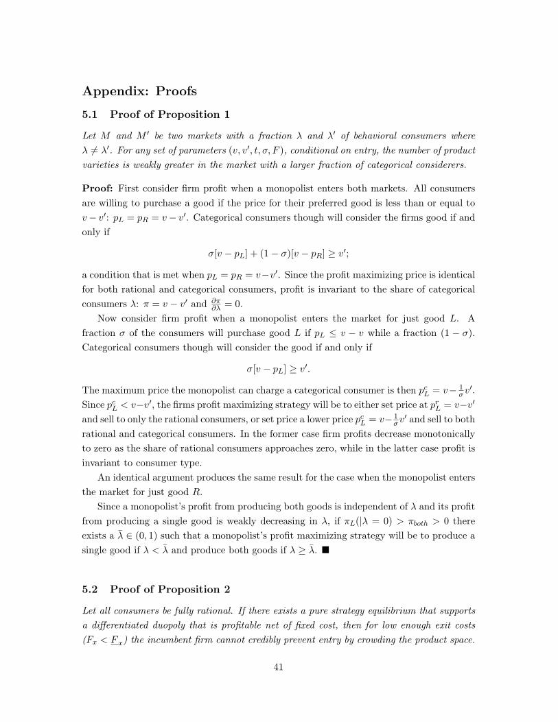
Appendix: Proofs

5.1 Proof of Proposition 1

Let M and M ′ be two markets with a fraction λ and λ′ of behavioral consumers whereλ 6= λ′. For any set of parameters (v, v′, t, σ, F ), conditional on entry, the number of productvarieties is weakly greater in the market with a larger fraction of categorical considerers.

Proof: First consider firm profit when a monopolist enters both markets. All consumersare willing to purchase a good if the price for their preferred good is less than or equal tov− v′: pL = pR = v− v′. Categorical consumers though will consider the firms good if andonly if

σ[v − pL] + (1− σ)[v − pR] ≥ v′;

a condition that is met when pL = pR = v−v′. Since the profit maximizing price is identicalfor both rational and categorical consumers, profit is invariant to the share of categoricalconsumers λ: π = v − v′ and ∂π

∂λ = 0.Now consider firm profit when a monopolist enters the market for just good L. A

fraction σ of the consumers will purchase good L if pL ≤ v − v while a fraction (1 − σ).Categorical consumers though will consider the good if and only if

σ[v − pL] ≥ v′.

The maximum price the monopolist can charge a categorical consumer is then pcL = v− 1

σv′.Since pc

L < v−v′, the firms profit maximizing strategy will be to either set price at prL = v−v′

and sell to only the rational consumers, or set price a lower price pcL = v− 1

σv′ and sell to bothrational and categorical consumers. In the former case firm profits decrease monotonicallyto zero as the share of rational consumers approaches zero, while in the latter case profit isinvariant to consumer type.

An identical argument produces the same result for the case when the monopolist entersthe market for just good R.

Since a monopolist’s profit from producing both goods is independent of λ and its profitfrom producing a single good is weakly decreasing in λ, if πL(|λ = 0) > πboth > 0 thereexists a λ ∈ (0, 1) such that a monopolist’s profit maximizing strategy will be to produce asingle good if λ < λ and produce both goods if λ ≥ λ. �

5.2 Proof of Proposition 2

Let all consumers be fully rational. If there exists a pure strategy equilibrium that supportsa differentiated duopoly that is profitable net of fixed cost, then for low enough exit costs(Fx < F x) the incumbent firm cannot credibly prevent entry by crowding the product space.

41

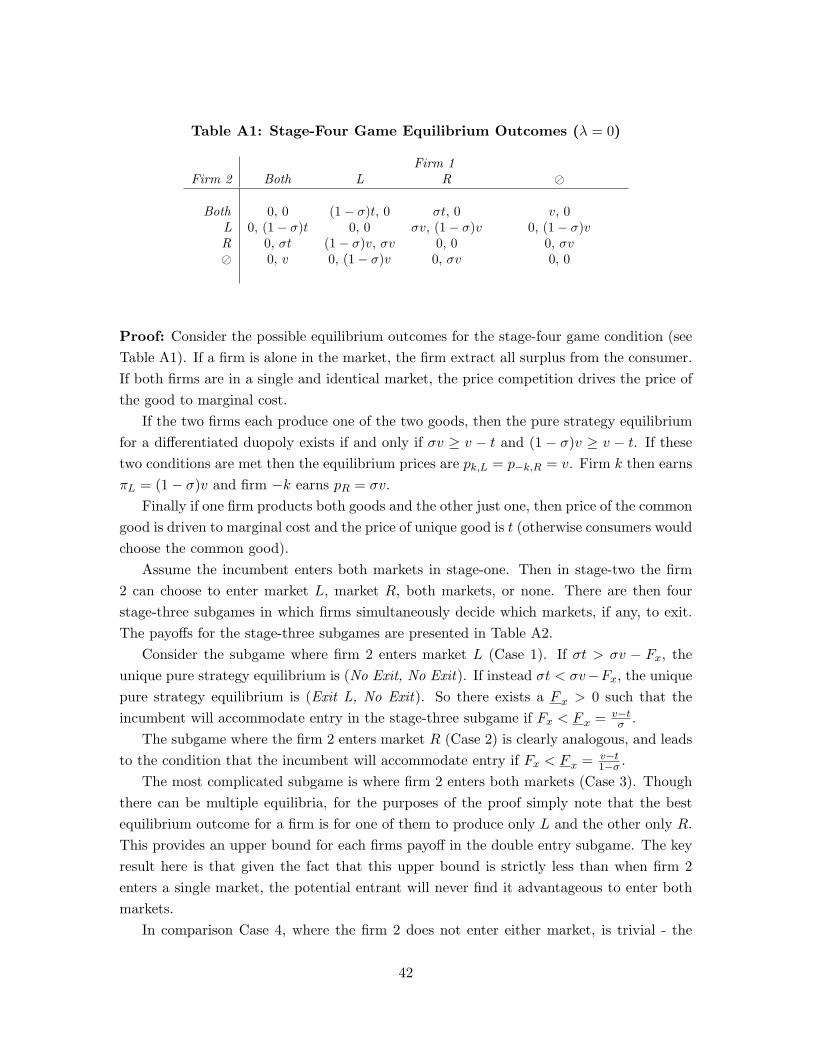
Table A1: Stage-Four Game Equilibrium Outcomes (λ = 0)

Firm 1Firm 2 Both L R �

Both 0, 0 (1− σ)t, 0 σt, 0 v, 0L 0, (1− σ)t 0, 0 σv, (1− σ)v 0, (1− σ)vR 0, σt (1− σ)v, σv 0, 0 0, σv� 0, v 0, (1− σ)v 0, σv 0, 0

Proof: Consider the possible equilibrium outcomes for the stage-four game condition (seeTable A1). If a firm is alone in the market, the firm extract all surplus from the consumer.If both firms are in a single and identical market, the price competition drives the price ofthe good to marginal cost.

If the two firms each produce one of the two goods, then the pure strategy equilibriumfor a differentiated duopoly exists if and only if σv ≥ v − t and (1 − σ)v ≥ v − t. If thesetwo conditions are met then the equilibrium prices are pk,L = p−k,R = v. Firm k then earnsπL = (1− σ)v and firm −k earns pR = σv.

Finally if one firm products both goods and the other just one, then price of the commongood is driven to marginal cost and the price of unique good is t (otherwise consumers wouldchoose the common good).

Assume the incumbent enters both markets in stage-one. Then in stage-two the firm2 can choose to enter market L, market R, both markets, or none. There are then fourstage-three subgames in which firms simultaneously decide which markets, if any, to exit.The payoffs for the stage-three subgames are presented in Table A2.

Consider the subgame where firm 2 enters market L (Case 1). If σt > σv − Fx, theunique pure strategy equilibrium is (No Exit, No Exit). If instead σt < σv−Fx, the uniquepure strategy equilibrium is (Exit L, No Exit). So there exists a F x > 0 such that theincumbent will accommodate entry in the stage-three subgame if Fx < F x = v−t

σ .The subgame where the firm 2 enters market R (Case 2) is clearly analogous, and leads

to the condition that the incumbent will accommodate entry if Fx < F x = v−t1−σ .

The most complicated subgame is where firm 2 enters both markets (Case 3). Thoughthere can be multiple equilibria, for the purposes of the proof simply note that the bestequilibrium outcome for a firm is for one of them to produce only L and the other only R.This provides an upper bound for each firms payoff in the double entry subgame. The keyresult here is that given the fact that this upper bound is strictly less than when firm 2enters a single market, the potential entrant will never find it advantageous to enter bothmarkets.

In comparison Case 4, where the firm 2 does not enter either market, is trivial - the

42

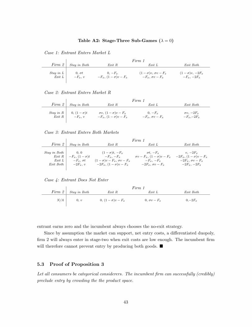
Table A2: Stage-Three Sub-Games (λ = 0)

Case 1: Entrant Enters Market L

Firm 1Firm 2 Stay in Both Exit R Exit L Exit Both

Stay in L 0, σt 0, −Fx (1 − σ)v, σv − Fx (1 − σ)v, −2Fx

Exit L −Fx, v −Fx, (1 − σ)v − Fx −Fx, σv − Fx −Fx, −2Fx

Case 2: Entrant Enters Market R

Firm 1Firm 2 Stay in Both Exit R Exit L Exit Both

Stay in R 0, (1 − σ)t σv, (1 − σ)v − Fx 0, −Fx σv, −2Fx

Exit R −Fx, v −Fx, (1 − σ)v − Fx −Fx, σv − Fx −Fx,−2Fx

Case 3: Entrant Enters Both Markets

Firm 1Firm 2 Stay in Both Exit R Exit L Exit Both

Stay in Both 0, 0 (1 − σ)t, −Fx σt, −Fx v, −2Fx

Exit R −Fx, (1 − σ)t −Fx, −Fx σv − Fx, (1 − σ)v − Fx −2Fx, (1 − σ)v − Fx

Exit L −Fx, σt (1 − σ)v − Fx, σv − Fx −Fx, −Fx −2Fx, σv − Fx

Exit Both −2Fx, v −2Fx, (1 − σ)v − Fx −2Fx, σv − Fx −2Fx, −2Fx

Case 4: Entrant Does Not Enter

Firm 1Firm 2 Stay in Both Exit R Exit L Exit Both

N/A 0, v 0, (1 − σ)v − Fx 0, σv − Fx 0,−2Fx

entrant earns zero and the incumbent always chooses the no-exit strategy.Since by assumption the market can support, net entry costs, a differentiated duopoly,

firm 2 will always enter in stage-two when exit costs are low enough. The incumbent firmwill therefore cannot prevent entry by producing both goods. �

5.3 Proof of Proposition 3

Let all consumers be categorical considerers. The incumbent firm can successfully (credibly)preclude entry by crowding the the product space.

43

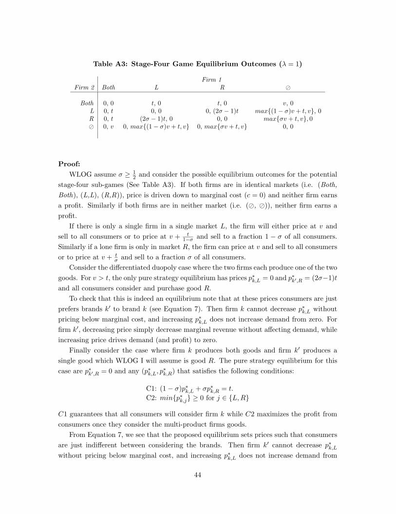
Table A3: Stage-Four Game Equilibrium Outcomes (λ = 1)

Firm 1Firm 2 Both L R �

Both 0, 0 t, 0 t, 0 v, 0L 0, t 0, 0 0, (2σ − 1)t max{(1− σ)v + t, v}, 0R 0, t (2σ − 1)t, 0 0, 0 max{σv + t, v}, 0� 0, v 0, max{(1− σ)v + t, v} 0, max{σv + t, v} 0, 0

Proof:WLOG assume σ ≥ 1

2 and consider the possible equilibrium outcomes for the potentialstage-four sub-games (See Table A3). If both firms are in identical markets (i.e. (Both,Both), (L,L), (R,R)), price is driven down to marginal cost (c = 0) and neither firm earnsa profit. Similarly if both firms are in neither market (i.e. (�, �)), neither firm earns aprofit.

If there is only a single firm in a single market L, the firm will either price at v andsell to all consumers or to price at v + t

1−σ and sell to a fraction 1 − σ of all consumers.Similarly if a lone firm is only in market R, the firm can price at v and sell to all consumersor to price at v + t

σ and sell to a fraction σ of all consumers.Consider the differentiated duopoly case where the two firms each produce one of the two

goods. For v > t, the only pure strategy equilibrium has prices p∗k,L = 0 and p∗k′,R = (2σ−1)tand all consumers consider and purchase good R.

To check that this is indeed an equilibrium note that at these prices consumers are justprefers brands k′ to brand k (see Equation 7). Then firm k cannot decrease p∗k,L withoutpricing below marginal cost, and increasing p∗k,L does not increase demand from zero. Forfirm k′, decreasing price simply decrease marginal revenue without affecting demand, whileincreasing price drives demand (and profit) to zero.

Finally consider the case where firm k produces both goods and firm k′ produces asingle good which WLOG I will assume is good R. The pure strategy equilibrium for thiscase are p∗k′,R = 0 and any (p∗k,L, p∗k,R) that satisfies the following conditions:

C1: (1− σ)p∗k,L + σp∗k,R = t.C2: min{p∗k,j} ≥ 0 for j ∈ {L,R}

C1 guarantees that all consumers will consider firm k while C2 maximizes the profit fromconsumers once they consider the multi-product firms goods.

From Equation 7, we see that the proposed equilibrium sets prices such that consumersare just indifferent between considering the brands. Then firm k′ cannot decrease p∗k,L

without pricing below marginal cost, and increasing p∗k,L does not increase demand from

44

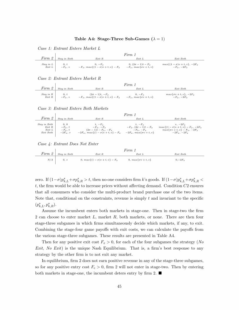
Table A4: Stage-Three Sub-Games (λ = 1)

Case 1: Entrant Enters Market LFirm 1

Firm 2 Stay in Both Exit R Exit L Exit Both

Stay in L 0, t 0, −Fx 0, (2σ − 1)t − Fx max{(1 − σ)v + t, v}, −2FxExit L −Fx, v −Fx, max{(1 − σ)v + t, v} − Fx −Fx, max{σv + t, v} −Fx, −2Fx

Case 2: Entrant Enters Market RFirm 1

Firm 2 Stay in Both Exit R Exit L Exit Both

Stay in R 0, t (2σ − 1)t, −Fx 0, −Fx max{σv + t, v}, −2FxExit R −Fx, v −Fx, max{(1 − σ)v + t, v} − Fx −Fx, max{σv + t, v} −Fx, −2Fx

Case 3: Entrant Enters Both MarketsFirm 1

Firm 2 Stay in Both Exit R Exit L Exit Both

Stay in Both 0, 0 t, −Fx t, −Fx v, −2FxExit R −Fx, t −Fx, −Fx −Fx, (2σ − 1)t − Fx max{(1 − σ)v + t, v} − Fx, −2FxExit L −Fx, t (2σ − 1)t − Fx, −Fx −Fx, −Fx max{σv + t, v} − Fx, −2Fx

Exit Both −2Fx, v −2Fx, max{(1 − σ)v + t, v} − Fx −2Fx, max{σv + t, v} −2Fx, −2Fx

Case 4: Entrant Does Not EnterFirm 1

Firm 2 Stay in Both Exit R Exit L Exit Both

N/A 0, v 0, max{(1 − σ)v + t, v} − Fx 0, max{σv + t, v} 0,−2Fx

zero. If (1−σ)p∗k,L+σp∗k,R > t, then no-one considers firm k’s goods. If (1−σ)p∗k,L+σp∗k,R <

t, the firm would be able to increase prices without affecting demand. Condition C2 ensuresthat all consumers who consider the multi-product brand purchase one of the two items.Note that, conditional on the constraints, revenue is simply t and invariant to the specific(p∗k,L, p∗k,R).

Assume the incumbent enters both markets in stage-one. Then in stage-two the firm2 can choose to enter market L, market R, both markets, or none. There are then fourstage-three subgames in which firms simultaneously decide which markets, if any, to exit.Combining the stage-four game payoffs with exit costs, we can calculate the payoffs fromthe various stage-three subgames. These results are presented in Table A4.

Then for any positive exit cost Fx > 0, for each of the four subgames the strategy (NoExit, No Exit) is the unique Nash Equilibrium. That is, a firm’s best response to anystrategy by the other firm is to not exit any market.

In equilibrium, firm 2 does not earn positive revenue in any of the stage-three subgames,so for any positive entry cost Fe > 0, firm 2 will not enter in stage-two. Then by enteringboth markets in stage-one, the incumbent deters entry by firm 2. �

45

5.4 Proof of Proposition 7

Suppose a fraction λ of consumers are categorical considerers. If there exists a pure strategyequilibrium that supports a differentiated oligopoly, then there exists an F > 0 such thatfor F < F Toyota will differentiate its products through the creation of an uninformativesecond brand.

Proof: If all consumers were rational, the set of prices (pM , p′M , pH , p′H) = (vM , vM , vH , vH))where each brand sells to the consumers that prefer their brand is a pure strategy equilib-rium. Toyota’s revenues are then

πr(λ = 0) = vM+vH2 − c.

To check that this is a pure strategy equilibrium, first note that in each market the afirm cannot increase price (otherwise demand goes to zero). If the a firm decrease it’s priceby t, it can exactly double demand. So if 1

2(vM −c) ≥ vM −c− t and 12(vH−c) ≥ vH−c− t,

the proposed strategy is an equilibrium.Consider next the case where one of these two conditions is not met. Then if one firm

sets price pj,k > c + t, the other firm (k′) in the market has an incentive to undercut theprice by t and capture all the consumers so both firms will want to price t above marginalcost. But there cannot be a symmetric equilibrium since for any price pj,k, the firm (k′)can increase price to pj,k + t without affecting demand.

Categorical consumers will consider only one category of goods. If Toyota sells itscars under one brand, then categorical consumers partition cars into mid-range brandsSM = {M,M ′,H} and luxury brands SH = {H ′}. Since all the mid-range cars are in setSM as long as min{pM , p′M} ≤ v all consumers of type α = 0 will consider set SM .

For a consumer of type α = 1, the expected value of considering set SM and SM are

U(SM ) = v − t2 − pH , and

U(SH) = v − t2 − p′H ,

respectively. So if all consumers were categorical, the competitive equilibrium is pM =p′M = v, pH = p′H = c. Toyota’s profit is then

π(λ = 1) = vM − c.

For the more general case of λ ∈ (0, 1), it is only important to note that there are nopure strategy equilibria, and that for any mixed strategy π(λ) < vM+vH

2 −c for all λ ∈ (0, 1].That is under no mixed strategy can the firms extract the full surplus from consumers.

If Toyota sells its cars under a new brand, then categorical consumers partition intomid-range brands SM = {M,M ′} and luxury brands SH = {H,H ′}. Then consumers of

46

type α = 0 will consider set SM if min{pM , p′M} ≤ v, and similarly consumers of type α = 1will consider set SH if min{pH , p′H} ≤ v. Since the rational equilibrium prices satisfy theseconditions, if Toyota create a new brand, it will earn profits of

π(λ = 1) = vM+vH2 − c− F

where F is a one time fixed cost for creating a new brand, regardless of the share ofcategorical consumers (λ). That is if Toyota create a new brand it will earn π(λ) =vM+vH

2 − c− F for all λ ∈ [0, 1].If all consumers were categorical (λ = 1), Toyota would pay F to create a new brand if

F satisfies:

π(λ = 1) ≥ π(λ = 1) ⇒ F ≤ vH − c.

More generally, if F < vM+vH2 − c − π(λ) Toyota will choose to create a new brand. And

since π(λ) < vM+vH2 − c for λ > 0, there exits a F > 0 such that for F < F , Toyota has

incentive to pay to create a new brand. �

47