Embed Size (px)
Citation preview
Better Risk Information for Smarter Investments
CATASTROPHE RISK ASSESSMENT METHODOLOGY
© 2013 The International Bank for Reconstruction and Development/The World Bank
1818 H Street NWWashington DC 20433Telephone: 202-473-1000Internet: www.worldbank.org
All rights reserved
This publication is a product of the staff of the International Bank for Reconstruction and Development/The World Bank. The findings, interpretations, and conclusions expressed in this volume do not necessarily reflect the views of the Executive Directors of The World Bank or the governments they represent.
The World Bank does not guarantee the accuracy of the data included in this work. The boundaries, colors, denominations, and other information shown on any map in this work do not imply any judgment on the part of The World Bank concerning the legal status of any territory or the endorsement or acceptance of such boundaries.
Rights and PermissionsThe material in this publication is copyrighted. Copying and/or transmitting portions or all of this work without permission may be a violation of applicable law. The International Bank for Reconstruction and Development/The World Bank encourages dissemination of its work and will normally grant permission to reproduce portions of the work promptly.
For permission to photocopy or reprint any part of this work, please send a request with complete information to the Copyright Clearance Center Inc., 222 Rosewood Drive, Danvers, MA 01923, USA; telephone: 978-750-8400; fax: 978-750-4470; Internet: www.copyright.com.
All other queries on rights and licenses, including subsidiary rights, should be addressed to the Office of the Publisher, The World Bank, 1818 H Street NW, Washington, DC 20433.
Designer: Miki Fernandez
Risk Assessment - Summary Report
Pacific Catastrophe Risk Assessment and Financing Initiative (PCRAFI)
Better Risk Information for Smarter Investments

CATASTROPHE RISK ASSESSMENT METHODOLOGY 3
Acknowledgements
The Pacific Catastrophe Risk Assessment and Financing Initiative (PCRAFI) is a joint initiative between the World Bank, the Secretariat of the Pacific Community through its Applied Geoscience & Technology Division (SPC/SOPAC), and the Asian Development Bank, with financial support from the Government of Japan, the
Global Facility for Disaster Reduction and Recovery (GFDRR), the European Union (ACP-EU) and with technical inputs from GNS Science, Geoscience Australia, and AIR Worldwide.
This report has been prepared by a World Bank team led by Iain Shuker and Olivier Mahul, comprising of Michael Bonte-Grapentin, Emilia Battaglini, Abigail Baca, Sandra Schuster, Cynthia Dharmajaya, and Sevara Atamuratova; an SPC/SOPAC team led by Mosese Sikivou, comprising of Litea Biukoto and Samantha Cook, and an ADB team led by Edy Brotoisworo and Jay Roop. The technical materials used in this report were produced by a team from AIR Worldwide led by Paolo Bazzurro, comprising Jaesung Park, Ivan Gomez, Bishwa Pandey, Daniel Duggan, Brent Poliquin and Yufang Rong. A team from GNS Science New Zealand led by Phil Glassey, provided ground truthing to the data used in the analysis. A team from Geoscience Australia, comprising of John Schneider and Alanna Simpson, provided technical support and advice throughout the project.
The report greatly benefited from data, information and other invaluable contributions made by the Pacific Island Countries, development partners, donor partners and private sector partners.
The team greatly appreciates the support and guidance received from Charles Feinstein, Ferid Belhaj, John Roome, Loic Chiquier, Francis Ghesquiere, and Abhas Jha.

Table of Contents
Acknowledgments ....................................................................................................................3
Executive Summary ....................................................................................................................7
Abbreviations and Acronyms .....................................................................................................9
Outline, Objectives and Outputs ..............................................................................................10
Catastrophe Risk Modeling ......................................................................................................12
1. Exposure Information ..........................................................................................................12
1.1 Population .....................................................................................................................12
1.2 Buildings .......................................................................................................................14
a. Locations .....................................................................................................................14
b. Field Surveys ................................................................................................................16
c. Occupancy Type and Construction Characteristics ........................................................18
d. Replacement Cost .......................................................................................................20
1.3 Infrastructure .................................................................................................................22
1.4 Crops ............................................................................................................................24
1.5 Replacement Costs by Country ......................................................................................30
2. Hazard Assessment ..............................................................................................................31
2.1 Tropical Cyclone Event Generation .................................................................................32
2.2 Tropical Cyclone Intensity Calculation ............................................................................35
a. Induced Winds ............................................................................................................35
b. Rainfall-Induced Inland Flood .......................................................................................38
c. Coastal Flood ...............................................................................................................39
2.3 Earthquake Event Generation ........................................................................................39
2.4 Earthquake Intensity Calculation ....................................................................................47
a. Ground Shaking ..........................................................................................................47
b. Tsunami Waves ............................................................................................................48
2.5 Ancillary GIS Data ..........................................................................................................50
3. Damage Estimation .............................................................................................................53
3.1 Consequence Database .................................................................................................53
a. Data Sources ...............................................................................................................53
b. Explanation of Data Fields ...........................................................................................55
c. Economic Loss Trending ...............................................................................................56
d. Database Statistics .......................................................................................................56
6 Pacific Catastrophe Risk Assessment and Financing Initiative (PCRAFI)
3.2 Damage Functions .........................................................................................................59
a. Buildings .....................................................................................................................60
b. Emergency Losses ........................................................................................................62
c. Infrastructure Assets ....................................................................................................63
d. Crops ..........................................................................................................................63
e. Fatalities and Injuries ...................................................................................................63
4. Country Catastrophe Risk Profiles ........................................................................................67
5. The Pacific Risk Information System (PacRIS) ........................................................................74
6. Applications ........................................................................................................................75
6.1 Post Disaster Response Capacity and Disaster Risk Financing ..........................................76
6.2 Disaster Risk Reduction and Urban/Infrastructure Spatial Planning ..................................76
6.3 Post-Disaster Assistance and Assessment .......................................................................76
6.4 Early Warning Systems and DRR Communication ...........................................................77
6.5 Reporting and Monitoring Agencies ..............................................................................77
7. References ...........................................................................................................................78
Annex A: Field Survey Locations ...............................................................................................79
Annex B: Building Locations (Level 4 Methodology) .................................................................81
Annex C: Construction Type ....................................................................................................85
Annex D: Infrastructure Exposure Database ..............................................................................87
Annex E: Example of Consequence Database ...........................................................................89
Annex F: Country Risk Profiles .................................................................................................91
CATASTROPHE RISK ASSESSMENT METHODOLOGY 7
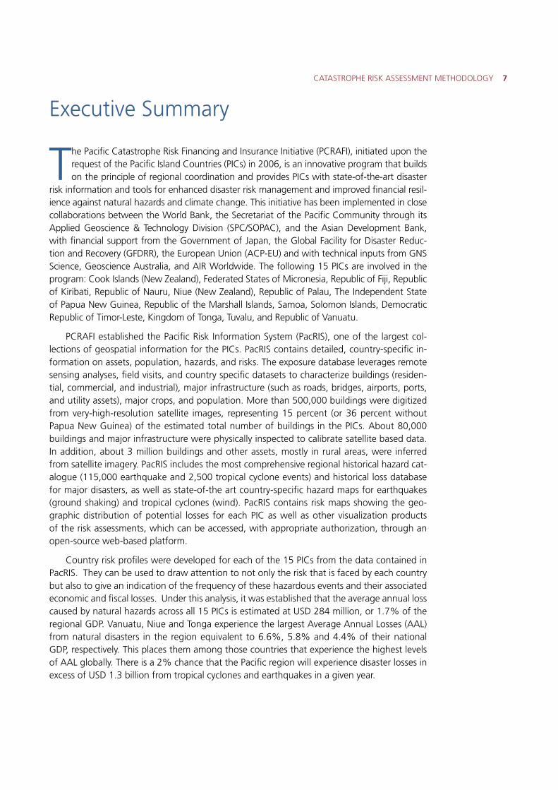
Executive Summary
The Pacific Catastrophe Risk Financing and Insurance Initiative (PCRAFI), initiated upon the request of the Pacific Island Countries (PICs) in 2006, is an innovative program that builds on the principle of regional coordination and provides PICs with state-of-the-art disaster
risk information and tools for enhanced disaster risk management and improved financial resil-ience against natural hazards and climate change. This initiative has been implemented in close collaborations between the World Bank, the Secretariat of the Pacific Community through its Applied Geoscience & Technology Division (SPC/SOPAC), and the Asian Development Bank, with financial support from the Government of Japan, the Global Facility for Disaster Reduc-tion and Recovery (GFDRR), the European Union (ACP-EU) and with technical inputs from GNS Science, Geoscience Australia, and AIR Worldwide. The following 15 PICs are involved in the program: Cook Islands (New Zealand), Federated States of Micronesia, Republic of Fiji, Republic of Kiribati, Republic of Nauru, Niue (New Zealand), Republic of Palau, The Independent State of Papua New Guinea, Republic of the Marshall Islands, Samoa, Solomon Islands, Democratic Republic of Timor-Leste, Kingdom of Tonga, Tuvalu, and Republic of Vanuatu.
PCRAFI established the Pacific Risk Information System (PacRIS), one of the largest col-lections of geospatial information for the PICs. PacRIS contains detailed, country-specific in-formation on assets, population, hazards, and risks. The exposure database leverages remote sensing analyses, field visits, and country specific datasets to characterize buildings (residen-tial, commercial, and industrial), major infrastructure (such as roads, bridges, airports, ports, and utility assets), major crops, and population. More than 500,000 buildings were digitized from very-high-resolution satellite images, representing 15 percent (or 36 percent without Papua New Guinea) of the estimated total number of buildings in the PICs. About 80,000 buildings and major infrastructure were physically inspected to calibrate satellite based data. In addition, about 3 million buildings and other assets, mostly in rural areas, were inferred from satellite imagery. PacRIS includes the most comprehensive regional historical hazard cat-alogue (115,000 earthquake and 2,500 tropical cyclone events) and historical loss database for major disasters, as well as state-of-the art country-specific hazard maps for earthquakes (ground shaking) and tropical cyclones (wind). PacRIS contains risk maps showing the geo-graphic distribution of potential losses for each PIC as well as other visualization products of the risk assessments, which can be accessed, with appropriate authorization, through an open-source web-based platform.
Country risk profiles were developed for each of the 15 PICs from the data contained in PacRIS. They can be used to draw attention to not only the risk that is faced by each country but also to give an indication of the frequency of these hazardous events and their associated economic and fiscal losses. Under this analysis, it was established that the average annual loss caused by natural hazards across all 15 PICs is estimated at USD 284 million, or 1.7% of the regional GDP. Vanuatu, Niue and Tonga experience the largest Average Annual Losses (AAL) from natural disasters in the region equivalent to 6.6%, 5.8% and 4.4% of their national GDP, respectively. This places them among those countries that experience the highest levels of AAL globally. There is a 2% chance that the Pacific region will experience disaster losses in excess of USD 1.3 billion from tropical cyclones and earthquakes in a given year.
8 Pacific Catastrophe Risk Assessment and Financing Initiative (PCRAFI)
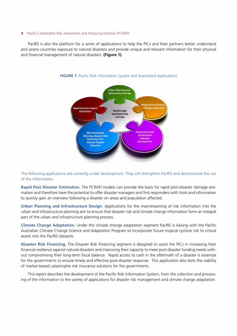
PacRIS is also the platform for a series of applications to help the PICs and their partners better understand and assess countries exposure to natural disasters and provide unique and relevant information for their physical and financial management of natural disasters. (Figure 1).
FIGURE 1. Pacific Risk Information System and Associated Applications
The following applications are currently under development. They will strengthen PacRIS and demonstrate the use of the information:
Rapid Post Disaster Estimation. The PCRAFI models can provide the basis for rapid post-disaster damage esti-mation and therefore have the potential to offer disaster managers and first responders with tools and information to quickly gain an overview following a disaster on areas and population affected.
Urban Planning and Infrastructure Design. Applications for the mainstreaming of risk information into the urban and infrastructure planning aim to ensure that disaster risk and climate change information form an integral part of the urban and infrastructure planning process.
Climate Change Adaptation. Under the climate change adaptation segment PacRIS is liaising with the Pacific Australian Climate Change Science and Adaptation Program to incorporate future tropical cyclone risk to critical assets into the PacRIS datasets.
Disaster Risk Financing. The Disaster Risk Financing segment is designed to assist the PICs in increasing their financial resilience against natural disasters and improving their capacity to meet post-disaster funding needs with-out compromising their long-term fiscal balance. Rapid access to cash in the aftermath of a disaster is essential for the governments to ensure timely and effective post-disaster response. This application also tests the viability of market-based catastrophe risk insurance solutions for the governments.
This report describes the development of the Pacific Risk Information System, from the collection and process-ing of the information to the variety of applications for disaster risk management and climate change adaptation.
CATASTROPHE RISK ASSESSMENT METHODOLOGY 9
Abbreviations and Acronyms
AAL Average Annual Loss
CCA Climate Change Adaptation
CK Cook Islands (New Zealand)
DF Damage Function
DR Damage Ratio
DRM Disaster Risk Management
FJ Republic of Fiji
FM Federated States of Micronesia
GDP Gross Domestic Product
GFDRR Global Facility for Disaster Reduction and Recovery
GIS Geographical Information System
IBTrACS International Best Tracks Archive for Climate Stewardship
KI Republic of Kiribati
LULC Land Use / Land Cover
MH Republic of the Marshall Islands
NR Republic of Nauru
NU Niue (New Zealand)
OpenDRI Open Data for Resilience Initiative
PacRIS Pacific Risk Information System
PCRAFI Pacific Catastrophe Risk Assessment and Financing Initiative
PG The Independent State of Papua New Guinea
PGA Peak Ground Acceleration
PICs Pacific Island Countries
PW Republic of Palau
SB Solomon Islands
SOPAC Applied Geoscience and Technology Division, SPC
SPC Secretariat of the Pacific Community
TL Democratic Republic of Timor-Leste
TO Kingdom of Tonga
TV Tuvalu
VU Republic of Vanuatu
WS Samoa
10 Pacific Catastrophe Risk Assessment and Financing Initiative (PCRAFI)
Outline, Objectives and Outputs
The Pacific Region is one of the most natural disaster prone regions on earth. The Pacific Island Countries (PICs) are highly exposed to the adverse effects of climate change and natural hazards, which can result in disasters affecting their entire eco-
nomic, human, and physical environment and impact their long-term development agenda. The average annual direct losses caused by natural disasters are estimated at US$284 million. Since 1950 natural disasters have affected approximately 9.2 million people in the Pacific Re-gion, causing 9,811 reported deaths. This has cost the PICs around US$3.2 billion (in nominal terms) in associated damage costs.
The primary objective of PCRAFI was to develop risk profiles for earthquakes (both ground shaking and tsunami) and tropical cyclones (wind and flood due to precipitation and storm surge) for the following 15 PICs1: Cook Islands (CK), Federated States of Micronesia (FM), Fiji (FJ), Kiribati (KI), Nauru (NR), Niue (NU), Palau (PW), Papua New Guinea (PG), Republic of the Marshall Islands (MH), Samoa (WS), Solomon Islands (SB), Timor-Leste (TL), Tonga (TO), Tuvalu (TV), and Vanuatu (VU).
This report focuses on the development of the country catastrophe risk profiles, the information collected, how it was catalogued and processed, and now being used for a variety of applications in Climate and Disaster Risk Management. The country risk profiles integrate data collected and produced through risk modeling and include maps showing the geographic distribution of assets and people at risk (Section 1), hazards assessed (Section 2) and potential monetary losses and casualties (Section 3). The profiles also include an analysis of the possible direct losses (in absolute terms and normalized by GDP) caused by tropical cyclones and earthquakes, and their impact though severe winds, rainfall, coastal storm surge, ground shaking and tsunami waves. The expected return period indicates the likelihood of a certain specified loss amount to be exceeded in any one year.
The country risk profiles developed can be used to improve the resilience of these 15 PICs to natural hazards and to help mitigate their tropical cyclone and earthquake risk (section 4). In addition, applications such as a risk information system and assessment tools were developed to better understand and assess the countries’ exposure to natural disasters. Disaster risk financing solutions and financial sector development (macroeconomic panning) are discussed. Further potential applications in disaster risk reduction and urban/infrastructure spatial planning, post disaster assistance and assessment, early warning systems and communications are described (Section 5).
1 For the purpose of this document the countries included in the initiative are referred to as the 15 PICs.
This report focuses on the
development of the country catastrophe
risk profiles, the information
collected, how it was catalogued and processed, and now being
used for a variety of applications in Climate and
Disaster Risk Management.
CATASTROPHE RISK ASSESSMENT METHODOLOGY 11CACATATAASTSTSTROROOR PHPHPHEE E E RIRIRIRISKSKSKSK A A AASSSSSS ESESSMSMSMMENENENENT T T MEMEMMETHHTHODODODDOLOLOLO OGOGOGY Y 111
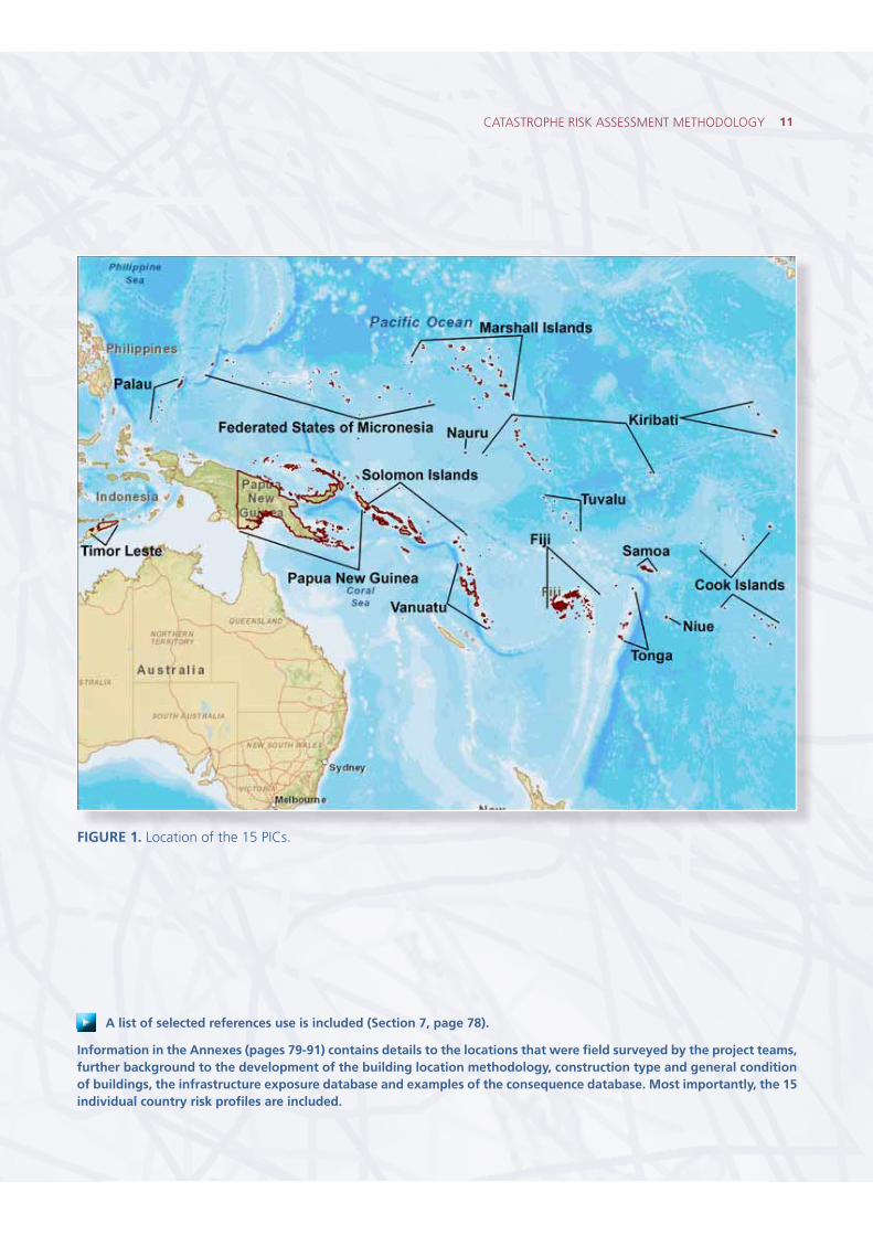
FIGURE 1. Location of the 15 PICs.
A list of selected references use is included (Section 7, page 78).
Information in the Annexes (pages 79-91) contains details to the locations that were field surveyed by the project teams, further background to the development of the building location methodology, construction type and general condition of buildings, the infrastructure exposure database and examples of the consequence database. Most importantly, the 15 individual country risk profiles are included.
��������������������������
12 Pacific Catastrophe Risk Assessment and Financing Initiative (PCRAFI)
Catastrophe Risk Modeling
Tropical cyclones and earthquakes are the most prominent natural hazards in the Pacific Islands Region. This study considers the devastating effects of wind, flood, and storm surge induced by tropical cyclones as well as earthquake ground shaking and
tsunamis. Other hazards, such as weaker but still potentially damaging local storms and vol-canic eruptions, are not included in this study. The risk due to tropical cyclones and tsunamis is computed assuming current climate conditions and sea levels. The effects of climate change on risk, which can be addressed using a similar methodology, are left to future investigations.
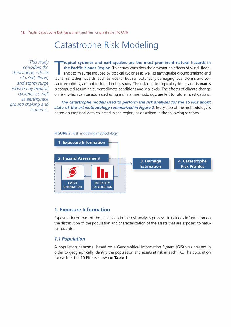
The catastrophe models used to perform the risk analyses for the 15 PICs adopt state-of-the-art methodology summarized in Figure 2. Every step of the methodology is based on empirical data collected in the region, as described in the following sections.
FIGURE 2. Risk modeling methodology
1. Exposure Information
Exposure forms part of the initial step in the risk analysis process. It includes information on the distribution of the population and characterization of the assets that are exposed to natu-ral hazards.
1.1 Population
A population database, based on a Geographical Information System (GIS) was created in order to geographically identify the population and assets at risk in each PIC. The population for each of the 15 PICs is shown in Table 1.
2. Hazard Assessment3. Damage Estimation
4. Catastrophe Risk Profiles
EVENTGENERATION
INTENSITYCALCULATION
INTENSITYCALCULATION
INTENSITYCALCULATION
1. Exposure Information
This study considers the
devastating effects of wind, flood,
and storm surge induced by tropical
cyclones as well as earthquake
ground shaking and tsunamis.
CATASTROPHE RISK ASSESSMENT METHODOLOGY 13
TABLE 1. Population projection for 2010 and administrative boundaries (resolution level) with census year and growth rates for each PIC
Country 2010 Projected Population
Census Year
SPC Annual Growth Rate Administrative Boundary Levels
CK 19,800 2006 0.32% Group Island Electoral Boundary Census District Enumeration Area
FJ 846,800 2007 0.46% Province Tikina Enumeration Area - -FM 111,600 2000 0.42% State Municipality Electoral District - -KI 101,400 2005 1.85% Group Island Village - -
MH 54,800 1999 0.69% Atoll Islet - - -NR 10,800 2006 2.08% Island District - - -NU 1,500 2006 -2.31% Village - - - -PG 6,405,600 2000 2.13% Province District Local Government
LevelCensus Unit -
PW 20,500 2005 0.59% State Hamlet - - -SB 547,500 1999 2.69% Province Ward Enumeration Area - -TL 1,066,600 2004 2.41% District Subdistrict Suco - -TO 103,400 2006 0.33% Division District Village Census Block -TV 10,000 2002 0.51% Island Village - - -VU 245,900 1999 2.54% Province Island Area Council Enumeration
Area-
WS 182,900 2006 0.30% Island Region District Village -
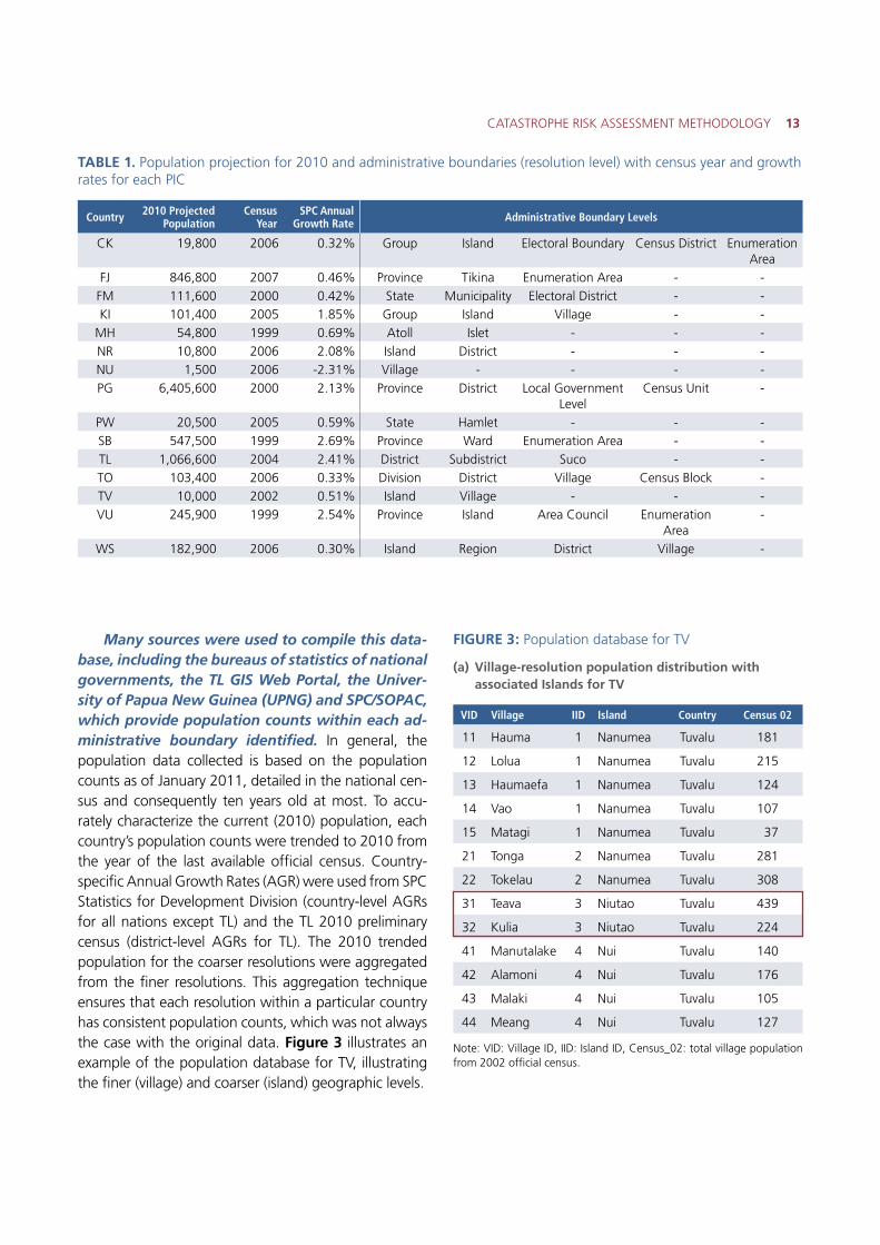
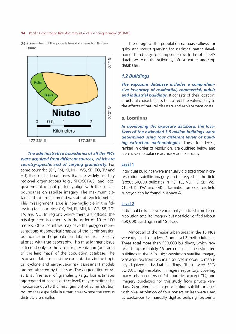
Many sources were used to compile this data-base, including the bureaus of statistics of national governments, the TL GIS Web Portal, the Univer-sity of Papua New Guinea (UPNG) and SPC/SOPAC, which provide population counts within each ad-ministrative boundary identified. In general, the population data collected is based on the population counts as of January 2011, detailed in the national cen-sus and consequently ten years old at most. To accu-rately characterize the current (2010) population, each country’s population counts were trended to 2010 from the year of the last available official census. Country-specific Annual Growth Rates (AGR) were used from SPC Statistics for Development Division (country-level AGRs for all nations except TL) and the TL 2010 preliminary census (district-level AGRs for TL). The 2010 trended population for the coarser resolutions were aggregated from the finer resolutions. This aggregation technique ensures that each resolution within a particular country has consistent population counts, which was not always the case with the original data. Figure 3 illustrates an example of the population database for TV, illustrating the finer (village) and coarser (island) geographic levels.
FIGURE 3: Population database for TV
(a) Village-resolution population distribution with associated Islands for TV
VID Village IID Island Country Census 02
11 Hauma 1 Nanumea Tuvalu 181
12 Lolua 1 Nanumea Tuvalu 215
13 Haumaefa 1 Nanumea Tuvalu 124
14 Vao 1 Nanumea Tuvalu 107
15 Matagi 1 Nanumea Tuvalu 37
21 Tonga 2 Nanumea Tuvalu 281
22 Tokelau 2 Nanumea Tuvalu 308
31 Teava 3 Niutao Tuvalu 439
32 Kulia 3 Niutao Tuvalu 224
41 Manutalake 4 Nui Tuvalu 140
42 Alamoni 4 Nui Tuvalu 176
43 Malaki 4 Nui Tuvalu 105
44 Meang 4 Nui Tuvalu 127
Note: VID: Village ID, IID: Island ID, Census_02: total village population from 2002 official census.
14 Pacific Catastrophe Risk Assessment and Financing Initiative (PCRAFI)
(b) Screenshot of the population database for Niutao Island
The administrative boundaries of all the PICs were acquired from different sources, which are country-specific and of varying granularity. For some countries (CK, FM, KI, MH, WS, SB, TO, TV and VU) the coastal boundaries that are widely used by regional organizations (e.g., SPC/SOPAC) and local government do not perfectly align with the coastal boundaries on satellite imagery. The maximum dis-tance of this misalignment was about two kilometers. This misalignment issue is non-negligible in the fol-lowing ten countries: CK, FM, FJ, MH, KI, WS, SB, TO, TV, and VU. In regions where there are offsets, the misalignment is generally in the order of 10 to 100 meters. Other countries may have the polygon repre-sentations (geometrical shapes) of the administration boundaries in the population database not perfectly aligned with true geography. This misalignment issue is limited only to the visual representation (and area of the land mass) of the population database. The exposure database and the computations in the tropi-cal cyclone and earthquake risk assessment models are not affected by this issue. The aggregation of re-sults at fine level of granularity (e.g., loss estimates aggregated at census district level) may sometimes be inaccurate due to the misalignment of administration boundaries especially in urban areas where the census districts are smaller.
The design of the population database allows for quick and robust querying for statistical metric devel-opment and easy superimposition with the other GIS databases, e.g., the buildings, infrastructure, and crop databases.
1.2 Buildings
The exposure database includes a comprehen-sive inventory of residential, commercial, public and industrial buildings. It consists of their location, structural characteristics that affect the vulnerability to the effects of natural disasters and replacement costs.
a. Locations
In developing the exposure database, the loca-tions of the estimated 3.5 million buildings were determined using four different levels of build-ing extraction methodologies. These four levels, ranked in order of resolution, are outlined below and are chosen to balance accuracy and economy.
Level 1
Individual buildings were manually digitized from high-resolution satellite imagery and surveyed in the field (about 80,000 buildings in PG, TO, VU, TV, SB, WS, CK, FJ, KI, PW, and FM). Information on locations field surveyed can be found in Annex A.
Level 2
Individual buildings were manually digitized from high-resolution satellite imagery but not field verified (about 450,000 buildings in all 15 PICs).
Almost all of the major urban areas in the 15 PICs were digitized using level 1 and level 2 methodologies. These total more than 530,000 buildings, which rep-resent approximately 15 percent of all the estimated buildings in the PICs. High-resolution satellite imagery was acquired from two main sources in order to manu-ally digitized individual buildings. These were SPC/SOPAC’s high-resolution imagery repository, covering many urban centers of 14 countries (except TL), and imagery purchased for this study from private ven-dors. Geo-referenced high-resolution satellite images with pixel resolution of four meters or less were used as backdrops to manually digitize building footprints
CATASTROPHE RISK ASSESSMENT METHODOLOGY 15
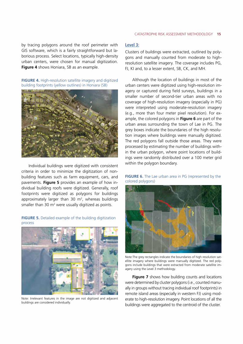
by tracing polygons around the roof perimeter with GIS software, which is a fairly straightforward but la-borious process. Select locations, typically high-density urban centers, were chosen for manual digitization. Figure 4 shows Honiara, SB as an example.
FIGURE 4. High-resolution satellite imagery and digitized building footprints (yellow outlines) in Honiara (SB)
Individual buildings were digitized with consistent criteria in order to minimize the digitization of non-building features such as farm equipment, cars, and pavements. Figure 5 provides an example of how in-dividual building roofs were digitized. Generally, roof footprints were digitized as polygons for buildings approximately larger than 30 m2, whereas buildings smaller than 30 m2 were usually digitized as points.
FIGURE 5. Detailed example of the building digitization process
Note: Irrelevant features in the image are not digitized and adjacent buildings are considered individually.
Level 3:
Clusters of buildings were extracted, outlined by poly-gons and manually counted from moderate to high-resolution satellite imagery. The coverage includes PG, FJ, KI and, to a lesser extent, SB, CK, and MH.
Although the location of buildings in most of the urban centers were digitized using high-resolution im-agery or captured during field surveys, buildings in a smaller number of second-tier urban areas with no coverage of high-resolution imagery (especially in PG) were interpreted using moderate-resolution imagery (e.g., more than four meter pixel resolution). For ex-ample, the colored polygons in Figure 6 are part of the urban areas surrounding the town of Lae in PG. The grey boxes indicate the boundaries of the high resolu-tion images where buildings were manually digitized. The red polygons fall outside those areas. They were processed by estimating the number of buildings with-in the urban polygon, where point locations of build-ings were randomly distributed over a 100 meter grid within the polygon boundary.
FIGURE 6. The Lae urban area in PG (represented by the colored polygons)
Note:The grey rectangles indicate the boundaries of high resolution sat-ellite imagery where buildings were manually digitized. The red poly-gons include buildings that were extracted from moderate satellite im-agery using the Level 3 methodology.
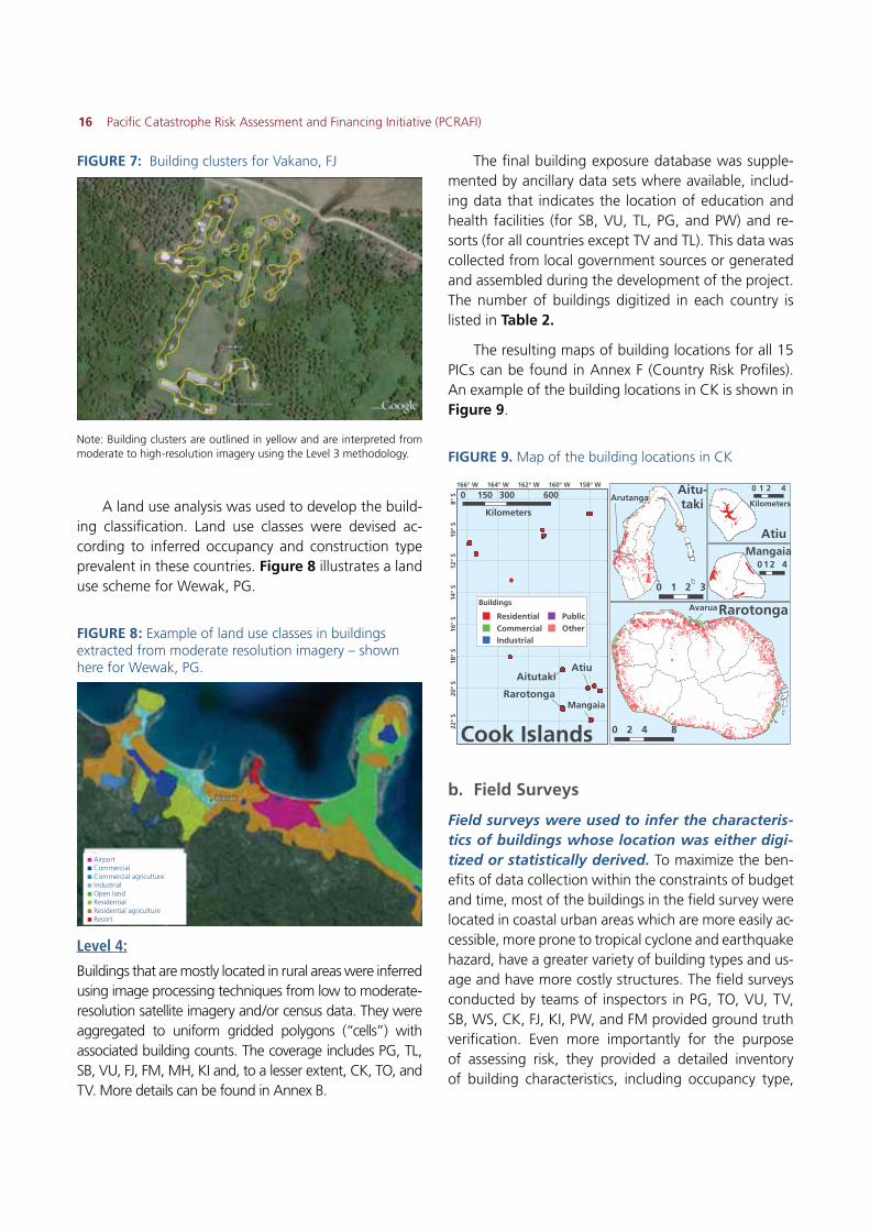
Figure 7 shows how building counts and locations were determined by cluster polygons (i.e., counted manu-ally in groups without tracing individual roof footprints) in remote island areas (especially in western FJ) using mod-erate to high-resolution imagery. Point locations of all the buildings were aggregated to the centroid of the cluster.
16 Pacific Catastrophe Risk Assessment and Financing Initiative (PCRAFI)
FIGURE 7: Building clusters for Vakano, FJ
Note: Building clusters are outlined in yellow and are interpreted from moderate to high-resolution imagery using the Level 3 methodology.
A land use analysis was used to develop the build-ing classification. Land use classes were devised ac-cording to inferred occupancy and construction type prevalent in these countries. Figure 8 illustrates a land use scheme for Wewak, PG.
FIGURE 8: Example of land use classes in buildings extracted from moderate resolution imagery – shown here for Wewak, PG.
Level 4:
Buildings that are mostly located in rural areas were inferred using image processing techniques from low to moderate-resolution satellite imagery and/or census data. They were aggregated to uniform gridded polygons (“cells”) with associated building counts. The coverage includes PG, TL, SB, VU, FJ, FM, MH, KI and, to a lesser extent, CK, TO, and TV. More details can be found in Annex B.
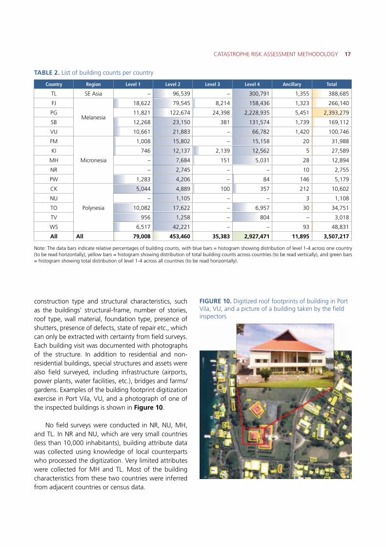
The final building exposure database was supple-mented by ancillary data sets where available, includ-ing data that indicates the location of education and health facilities (for SB, VU, TL, PG, and PW) and re-sorts (for all countries except TV and TL). This data was collected from local government sources or generated and assembled during the development of the project. The number of buildings digitized in each country is listed in Table 2.
The resulting maps of building locations for all 15 PICs can be found in Annex F (Country Risk Profiles). An example of the building locations in CK is shown in Figure 9.
FIGURE 9. Map of the building locations in CK
b. Field Surveys
Field surveys were used to infer the characteris-tics of buildings whose location was either digi-tized or statistically derived. To maximize the ben-efits of data collection within the constraints of budget and time, most of the buildings in the field survey were located in coastal urban areas which are more easily ac-cessible, more prone to tropical cyclone and earthquake hazard, have a greater variety of building types and us-age and have more costly structures. The field surveys conducted by teams of inspectors in PG, TO, VU, TV, SB, WS, CK, FJ, KI, PW, and FM provided ground truth verification. Even more importantly for the purpose of assessing risk, they provided a detailed inventory of building characteristics, including occupancy type,
� Airport� Commercial� Commercial agriculture� Industrial� Open land� Residential� Residential agriculture� Resort
AitutakiAtiu
MangaiaRarotonga
158° W160° W162° W164° W166° W
8° S
10°
S12
° S
14°
S16
° S
18°
S20
° S
22°
S
Avarua
Arutanga
0 4 82
Rarotonga
Atiu
Aitu- taki
Mangaia
0 300 600150
Kilometers
Cook Islands
0 2 41
0 2 41
Kilometers
0 1 2 3Buildings
ResidentialCommercialIndustrial
PublicOther
CATASTROPHE RISK ASSESSMENT METHODOLOGY 17
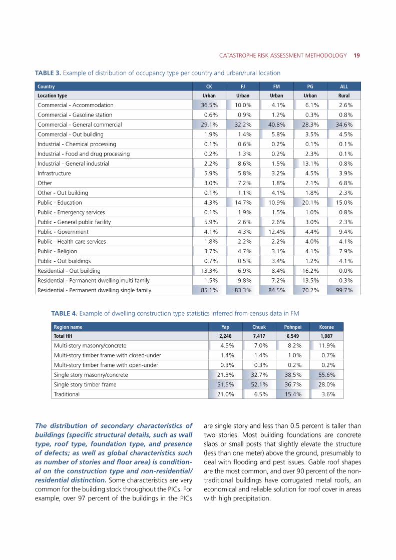
construction type and structural characteristics, such as the buildings’ structural-frame, number of stories, roof type, wall material, foundation type, presence of shutters, presence of defects, state of repair etc., which can only be extracted with certainty from field surveys. Each building visit was documented with photographs of the structure. In addition to residential and non-residential buildings, special structures and assets were also field surveyed, including infrastructure (airports, power plants, water facilities, etc.), bridges and farms/gardens. Examples of the building footprint digitization exercise in Port Vila, VU, and a photograph of one of the inspected buildings is shown in Figure 10.
No field surveys were conducted in NR, NU, MH, and TL. In NR and NU, which are very small countries (less than 10,000 inhabitants), building attribute data was collected using knowledge of local counterparts who processed the digitization. Very limited attributes were collected for MH and TL. Most of the building characteristics from these two countries were inferred from adjacent countries or census data.
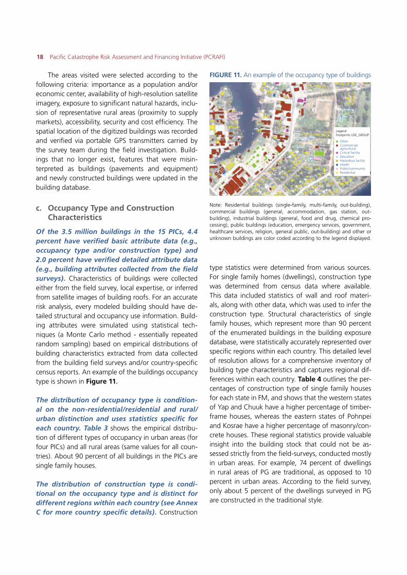
TABLE 2. List of building counts per country
Note: The data bars indicate relative percentages of building counts, with blue bars = histogram showing distribution of level 1-4 across one country (to be read horizontally), yellow bars = histogram showing distribution of total building counts across countries (to be read vertically), and green bars = histogram showing total distribution of level 1-4 across all countries (to be read horizontally).
Country Region Level 1 Level 2 Level 3 Level 4 Ancillary Total
TL SE Asia – 96,539 – 300,791 1,355 388,685
FJ
Melanesia
18,622 79,545 8,214 158,436 1,323 266,140
PG 11,821 122,674 24,398 2,228,935 5,451 2,393,279
SB 12,268 23,150 381 131,574 1,739 169,112
VU 10,661 21,883 – 66,782 1,420 100,746
FM
Micronesia
1,008 15,802 – 15,158 20 31,988
KI 746 12,137 2,139 12,562 5 27,589
MH – 7,684 151 5,031 28 12,894
NR – 2,745 – – 10 2,755
PW 1,283 4,206 – 84 146 5,179
CK
Polynesia
5,044 4,889 100 357 212 10,602
NU – 1,105 – – 3 1,108
TO 10,082 17,622 – 6,957 30 34,751
TV 956 1,258 – 804 – 3,018
WS 6,517 42,221 – – 93 48,831
All All 79,008 453,460 35,383 2,927,471 11,895 3,507,217
FIGURE 10. Digitized roof footprints of building in Port Vila, VU, and a picture of a building taken by the field inspectors
18 Pacific Catastrophe Risk Assessment and Financing Initiative (PCRAFI)
The areas visited were selected according to the following criteria: importance as a population and/or economic center, availability of high-resolution satellite imagery, exposure to significant natural hazards, inclu-sion of representative rural areas (proximity to supply markets), accessibility, security and cost efficiency. The spatial location of the digitized buildings was recorded and verified via portable GPS transmitters carried by the survey team during the field investigation. Build-ings that no longer exist, features that were misin-terpreted as buildings (pavements and equipment) and newly constructed buildings were updated in the building database.
c. Occupancy Type and Construction Characteristics
Of the 3.5 million buildings in the 15 PICs, 4.4 percent have verified basic attribute data (e.g., occupancy type and/or construction type) and 2.0 percent have verified detailed attribute data (e.g., building attributes collected from the field surveys). Characteristics of buildings were collected either from the field survey, local expertise, or inferred from satellite images of building roofs. For an accurate risk analysis, every modeled building should have de-tailed structural and occupancy use information. Build-ing attributes were simulated using statistical tech-niques (a Monte Carlo method - essentially repeated random sampling) based on empirical distributions of building characteristics extracted from data collected from the building field surveys and/or country-specific census reports. An example of the buildings occupancy type is shown in Figure 11.
The distribution of occupancy type is condition-al on the non-residential/residential and rural/urban distinction and uses statistics specific for each country. Table 3 shows the empirical distribu-tion of different types of occupancy in urban areas (for four PICs) and all rural areas (same values for all coun-tries). About 90 percent of all buildings in the PICs are single family houses.
The distribution of construction type is condi-tional on the occupancy type and is distinct for different regions within each country (see Annex C for more country specific details). Construction
FIGURE 11. An example of the occupancy type of buildings
Note: Residential buildings (single-family, multi-family, out-building), commercial buildings (general, accommodation, gas station, out-building), industrial buildings (general, food and drug, chemical pro-cessing), public buildings (education, emergency services, government, healthcare services, religion, general public, out-building) and other or unknown buildings are color coded according to the legend displayed.
type statistics were determined from various sources. For single family homes (dwellings), construction type was determined from census data where available. This data included statistics of wall and roof materi-als, along with other data, which was used to infer the construction type. Structural characteristics of single family houses, which represent more than 90 percent of the enumerated buildings in the building exposure database, were statistically accurately represented over specific regions within each country. This detailed level of resolution allows for a comprehensive inventory of building type characteristics and captures regional dif-ferences within each country. Table 4 outlines the per-centages of construction type of single family houses for each state in FM, and shows that the western states of Yap and Chuuk have a higher percentage of timber-frame houses, whereas the eastern states of Pohnpei and Kosrae have a higher percentage of masonry/con-crete houses. These regional statistics provide valuable insight into the building stock that could not be as-sessed strictly from the field-surveys, conducted mostly in urban areas. For example, 74 percent of dwellings in rural areas of PG are traditional, as opposed to 10 percent in urban areas. According to the field survey, only about 5 percent of the dwellings surveyed in PG are constructed in the traditional style.
LegendFootprints USE_GROUP
� Other� Commercial/
agricultural� Critical facility� Education� Hazardous facility� Health� Public/community� Residential
CATASTROPHE RISK ASSESSMENT METHODOLOGY 19
Country CK FJ FM PG ALL
Location type Urban Urban Urban Urban Rural
Commercial - Accommodation 36.5% 10.0% 4.1% 6.1% 2.6%
Commercial - Gasoline station 0.6% 0.9% 1.2% 0.3% 0.8%
Commercial - General commercial 29.1% 32.2% 40.8% 28.3% 34.6%
Commercial - Out building 1.9% 1.4% 5.8% 3.5% 4.5%
Industrial - Chemical processing 0.1% 0.6% 0.2% 0.1% 0.1%
Industrial - Food and drug processing 0.2% 1.3% 0.2% 2.3% 0.1%
Industrial - General industrial 2.2% 8.6% 1.5% 13.1% 0.8%
Infrastructure 5.9% 5.8% 3.2% 4.5% 3.9%
Other 3.0% 7.2% 1.8% 2.1% 6.8%
Other - Out building 0.1% 1.1% 4.1% 1.8% 2.3%
Public - Education 4.3% 14.7% 10.9% 20.1% 15.0%
Public - Emergency services 0.1% 1.9% 1.5% 1.0% 0.8%
Public - General public facility 5.9% 2.6% 2.6% 3.0% 2.3%
Public - Government 4.1% 4.3% 12.4% 4.4% 9.4%
Public - Health care services 1.8% 2.2% 2.2% 4.0% 4.1%
Public - Religion 3.7% 4.7% 3.1% 4.1% 7.9%
Public - Out buildings 0.7% 0.5% 3.4% 1.2% 4.1%
Residential - Out building 13.3% 6.9% 8.4% 16.2% 0.0%
Residential - Permanent dwelling multi family 1.5% 9.8% 7.2% 13.5% 0.3%
Residential - Permanent dwelling single family 85.1% 83.3% 84.5% 70.2% 99.7%
TABLE 3. Example of distribution of occupancy type per country and urban/rural location
TABLE 4. Example of dwelling construction type statistics inferred from census data in FM
The distribution of secondary characteristics of buildings (specific structural details, such as wall type, roof type, foundation type, and presence of defects; as well as global characteristics such as number of stories and floor area) is condition-al on the construction type and non-residential/residential distinction. Some characteristics are very common for the building stock throughout the PICs. For example, over 97 percent of the buildings in the PICs
are single story and less than 0.5 percent is taller than two stories. Most building foundations are concrete slabs or small posts that slightly elevate the structure (less than one meter) above the ground, presumably to deal with flooding and pest issues. Gable roof shapes are the most common, and over 90 percent of the non-traditional buildings have corrugated metal roofs, an economical and reliable solution for roof cover in areas with high precipitation.
Region name Yap Chuuk Pohnpei Kosrae
Total HH 2,246 7,417 6,549 1,087
Multi-story masonry/concrete 4.5% 7.0% 8.2% 11.9%
Multi-story timber frame with closed-under 1.4% 1.4% 1.0% 0.7%
Multi-story timber frame with open-under 0.3% 0.3% 0.2% 0.2%
Single story masonry/concrete 21.3% 32.7% 38.5% 55.6%
Single story timber frame 51.5% 52.1% 36.7% 28.0%
Traditional 21.0% 6.5% 15.4% 3.6%
20 Pacific Catastrophe Risk Assessment and Financing Initiative (PCRAFI)
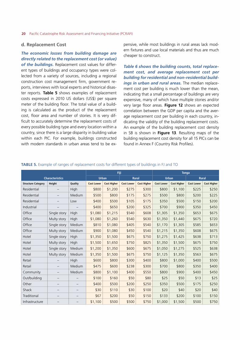
d. Replacement Cost
The economic losses from building damage are directly related to the replacement cost (or value) of the buildings. Replacement cost values for differ-ent types of buildings and occupancy types were col-lected from a variety of sources, including a regional construction cost management firm, government re-ports, interviews with local experts and historical disas-ter reports. Table 5 shows examples of replacement costs expressed in 2010 US dollars (US$) per square meter of the building floor. The total value of a build-ing is calculated as the product of the replacement cost, floor area and number of stories. It is very dif-ficult to accurately determine the replacement costs of every possible building type and every location within a country, since there is a large disparity in building value within each PIC. For example, buildings constructed with modern standards in urban areas tend to be ex-
pensive, while most buildings in rural areas lack mod-ern fixtures and use local materials and thus are much cheaper to construct.
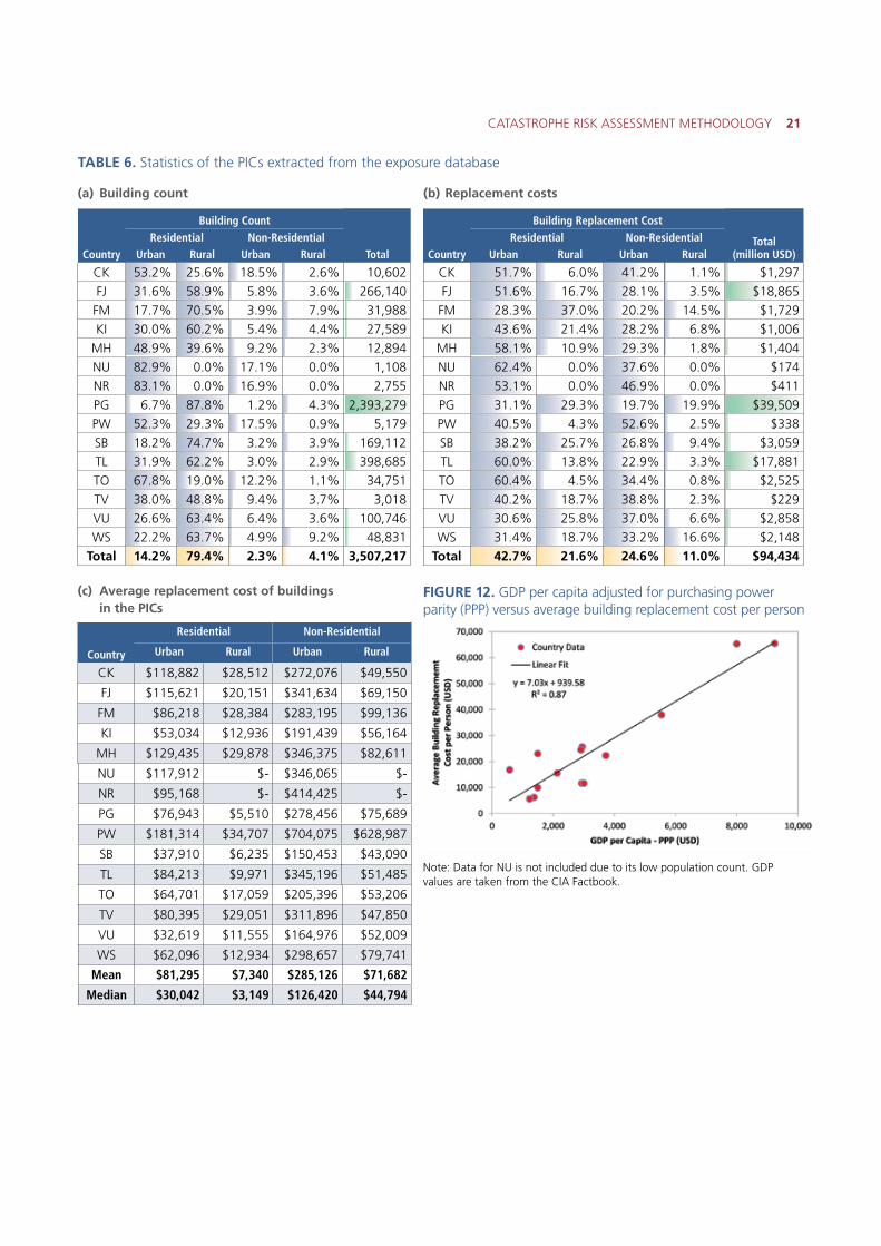
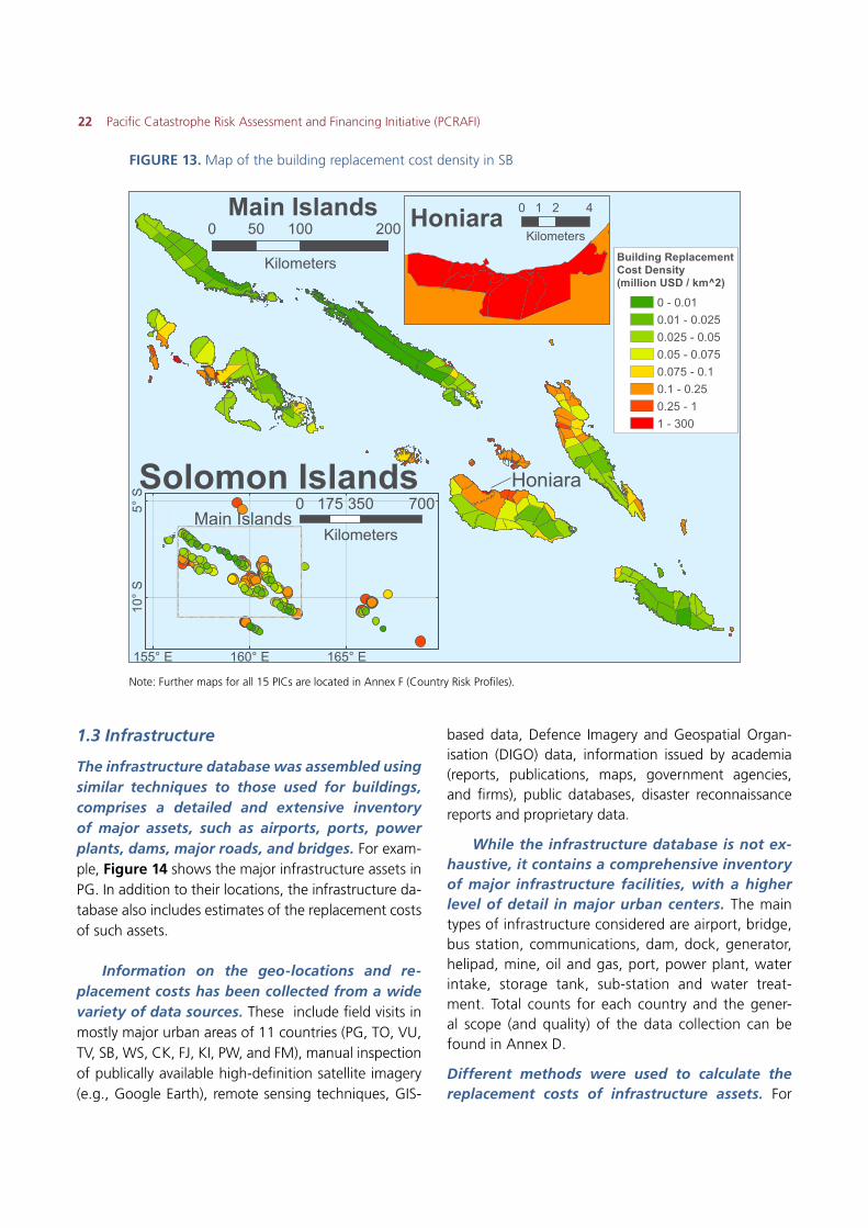
Table 6 shows the building counts, total replace-ment cost, and average replacement cost per building for residential and non-residential build-ings in urban and rural areas. The median replace-ment cost per building is much lower than the mean, indicating that a small percentage of buildings are very expensive, many of which have multiple stories and/or very large floor areas. Figure 12 shows an expected correlation between the GDP per capita and the aver-age replacement cost per building in each country, in-dicating the validity of the building replacement costs. An example of the building replacement cost density in SB is shown in Figure 13. Resulting maps of the building replacement cost density for all 15 PICs can be found in Annex F (Country Risk Profiles).
Characteristics
Fiji Tonga
Urban Rural Urban Rural
Structure Category Height Quality Cost Lower Cost Higher Cost Lower Cost Higher Cost Lower Cost Higher Cost Lower Cost Higher
Residential – High $800 $1,200 $275 $300 $800 $1,100 $225 $250
Residential – Medium $500 $800 $175 $275 $500 $800 $200 $225
Residential – Low $400 $500 $105 $175 $350 $500 $150 $200
Industrial – – $400 $650 $200 $325 $700 $900 $350 $450
Office Single story High $1,080 $1,215 $540 $608 $1,305 $1,350 $653 $675
Office Multy story High $1,080 $1,260 $540 $630 $1,350 $1,440 $675 $720
Office Single story Medium $810 $1,080 $405 $540 $1,170 $1,305 $585 $653
Office Multy story Medium $900 $1,080 $450 $540 $1,215 $1,350 $608 $675
Hotel Single story High $1,350 $1,500 $675 $750 $1,275 $1,425 $638 $713
Hotel Multy story High $1,500 $1,650 $750 $825 $1,350 $1,500 $675 $750
Hotel Single story Medium $1,200 $1,350 $600 $675 $1,050 $1,275 $525 $638
Hotel Multy story Medium $1,350 $1,500 $675 $750 $1,125 $1,350 $563 $675
Retail – High $600 $800 $300 $400 $800 $1,000 $400 $500
Retail – Medium $475 $600 $238 $300 $700 $800 $350 $400
Community – Medium $800 $1,100 $400 $550 $800 $900 $400 $450
Out/building – – $100 $160 $50 $80 $25 $50 $13 $25
Other – – $400 $500 $200 $250 $350 $500 $175 $250
Shack – – $30 $110 $30 $100 $20 $40 $20 $40
Traditional – – $67 $200 $50 $150 $133 $200 $100 $150
Infrastructure – – $1,100 $500 $500 $750 $1,000 $1,500 $500 $750
TABLE 5. Example of ranges of replacement costs for different types of buildings in FJ and TO
CATASTROPHE RISK ASSESSMENT METHODOLOGY 21
TABLE 6. Statistics of the PICs extracted from the exposure database
(a) Building count (b) Replacement costs
(c) Average replacement cost of buildings in the PICs
FIGURE 12. GDP per capita adjusted for purchasing power parity (PPP) versus average building replacement cost per person
Country
Building Count
TotalResidential Non-Residential
Urban Rural Urban Rural
CK 53.2% 25.6% 18.5% 2.6% 10,602
FJ 31.6% 58.9% 5.8% 3.6% 266,140
FM 17.7% 70.5% 3.9% 7.9% 31,988
KI 30.0% 60.2% 5.4% 4.4% 27,589
MH 48.9% 39.6% 9.2% 2.3% 12,894
NU 82.9% 0.0% 17.1% 0.0% 1,108
NR 83.1% 0.0% 16.9% 0.0% 2,755
PG 6.7% 87.8% 1.2% 4.3% 2,393,279
PW 52.3% 29.3% 17.5% 0.9% 5,179
SB 18.2% 74.7% 3.2% 3.9% 169,112
TL 31.9% 62.2% 3.0% 2.9% 398,685
TO 67.8% 19.0% 12.2% 1.1% 34,751
TV 38.0% 48.8% 9.4% 3.7% 3,018
VU 26.6% 63.4% 6.4% 3.6% 100,746
WS 22.2% 63.7% 4.9% 9.2% 48,831
Total 14.2% 79.4% 2.3% 4.1% 3,507,217
Country
Building Replacement Cost
Total (million USD)
Residential Non-ResidentialUrban Rural Urban Rural
CK 51.7% 6.0% 41.2% 1.1% $1,297
FJ 51.6% 16.7% 28.1% 3.5% $18,865
FM 28.3% 37.0% 20.2% 14.5% $1,729
KI 43.6% 21.4% 28.2% 6.8% $1,006
MH 58.1% 10.9% 29.3% 1.8% $1,404
NU 62.4% 0.0% 37.6% 0.0% $174
NR 53.1% 0.0% 46.9% 0.0% $411
PG 31.1% 29.3% 19.7% 19.9% $39,509
PW 40.5% 4.3% 52.6% 2.5% $338
SB 38.2% 25.7% 26.8% 9.4% $3,059
TL 60.0% 13.8% 22.9% 3.3% $17,881
TO 60.4% 4.5% 34.4% 0.8% $2,525
TV 40.2% 18.7% 38.8% 2.3% $229
VU 30.6% 25.8% 37.0% 6.6% $2,858
WS 31.4% 18.7% 33.2% 16.6% $2,148
Total 42.7% 21.6% 24.6% 11.0% $94,434
Country
Residential Non-Residential
Urban Rural Urban Rural
CK $118,882 $28,512 $272,076 $49,550
FJ $115,621 $20,151 $341,634 $69,150
FM $86,218 $28,384 $283,195 $99,136
KI $53,034 $12,936 $191,439 $56,164
MH $129,435 $29,878 $346,375 $82,611
NU $117,912 $- $346,065 $-
NR $95,168 $- $414,425 $-
PG $76,943 $5,510 $278,456 $75,689
PW $181,314 $34,707 $704,075 $628,987
SB $37,910 $6,235 $150,453 $43,090
TL $84,213 $9,971 $345,196 $51,485
TO $64,701 $17,059 $205,396 $53,206
TV $80,395 $29,051 $311,896 $47,850
VU $32,619 $11,555 $164,976 $52,009
WS $62,096 $12,934 $298,657 $79,741
Mean $81,295 $7,340 $285,126 $71,682
Median $30,042 $3,149 $126,420 $44,794
Note: Data for NU is not included due to its low population count. GDP values are taken from the CIA Factbook.
22 Pacific Catastrophe Risk Assessment and Financing Initiative (PCRAFI)
FIGURE 13. Map of the building replacement cost density in SB
Note: Further maps for all 15 PICs are located in Annex F (Country Risk Profiles).
1.3 Infrastructure
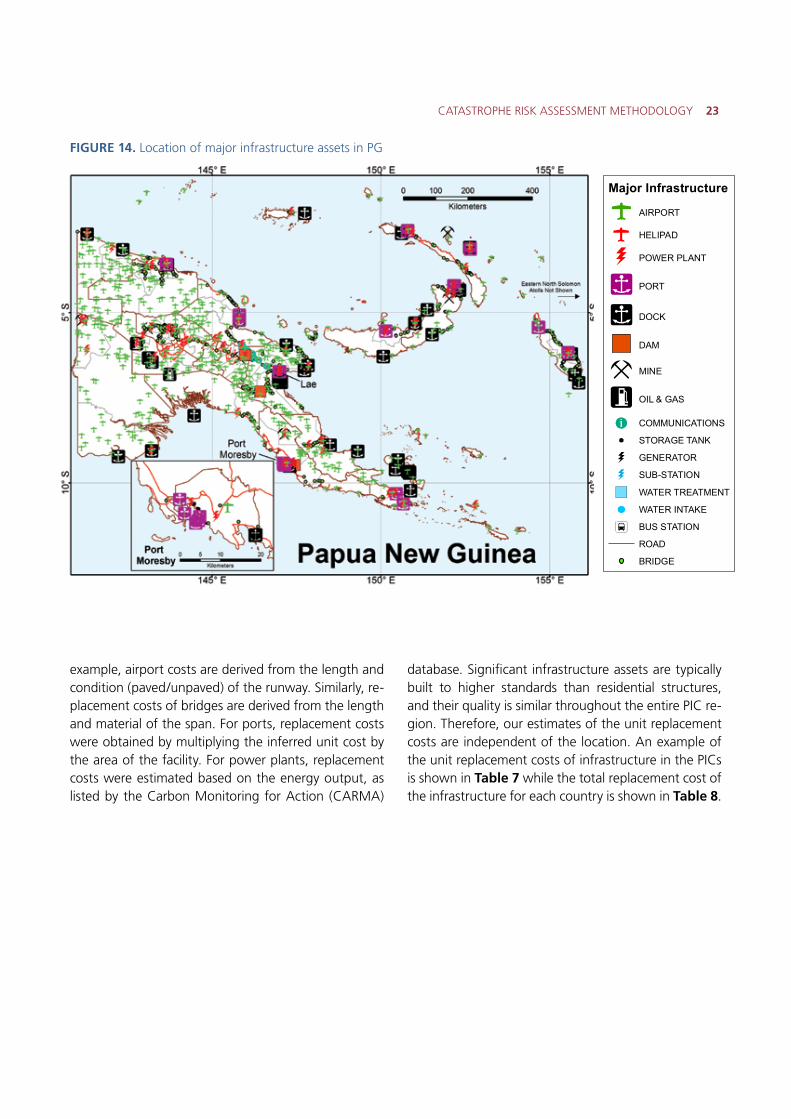
The infrastructure database was assembled using similar techniques to those used for buildings, comprises a detailed and extensive inventory of major assets, such as airports, ports, power plants, dams, major roads, and bridges. For exam-ple, Figure 14 shows the major infrastructure assets in PG. In addition to their locations, the infrastructure da-tabase also includes estimates of the replacement costs of such assets.
Information on the geo-locations and re-placement costs has been collected from a wide variety of data sources. These include field visits in mostly major urban areas of 11 countries (PG, TO, VU, TV, SB, WS, CK, FJ, KI, PW, and FM), manual inspection of publically available high-definition satellite imagery (e.g., Google Earth), remote sensing techniques, GIS-
based data, Defence Imagery and Geospatial Organ-isation (DIGO) data, information issued by academia (reports, publications, maps, government agencies, and firms), public databases, disaster reconnaissance reports and proprietary data.
While the infrastructure database is not ex-haustive, it contains a comprehensive inventory of major infrastructure facilities, with a higher level of detail in major urban centers. The main types of infrastructure considered are airport, bridge, bus station, communications, dam, dock, generator, helipad, mine, oil and gas, port, power plant, water intake, storage tank, sub-station and water treat-ment. Total counts for each country and the gener-al scope (and quality) of the data collection can be found in Annex D.
Different methods were used to calculate the replacement costs of infrastructure assets. For
165° E160° E155° E
5° S
10°
S
0 350 700175
Kilometers
Solomon Islands
0 100 20050
Kilometers
Main Islands
Main Islands
Honiara
Honiara 0 2 41
KilometersBuilding ReplacementCost Density(million USD / km^2)
0 - 0.010.01 - 0.0250.025 - 0.050.05 - 0.0750.075 - 0.10.1 - 0.250.25 - 11 - 300
CATASTROPHE RISK ASSESSMENT METHODOLOGY 23
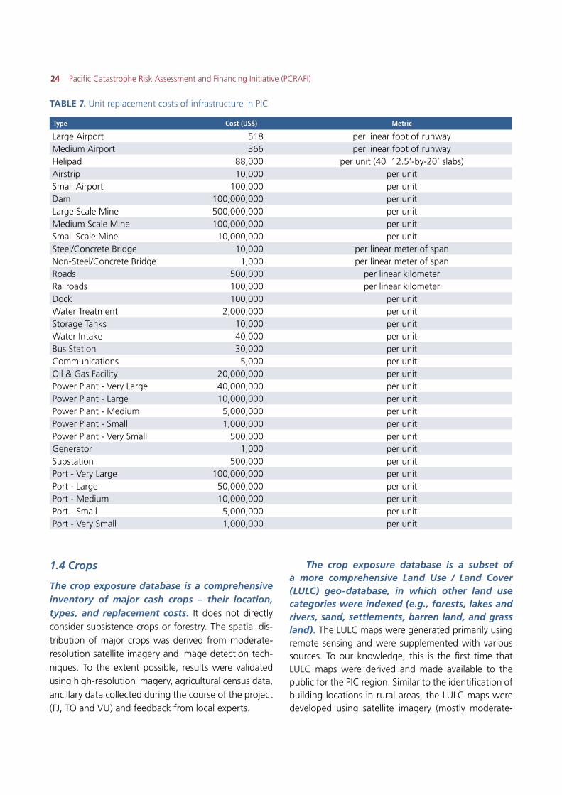
example, airport costs are derived from the length and condition (paved/unpaved) of the runway. Similarly, re-placement costs of bridges are derived from the length and material of the span. For ports, replacement costs were obtained by multiplying the inferred unit cost by the area of the facility. For power plants, replacement costs were estimated based on the energy output, as listed by the Carbon Monitoring for Action (CARMA)
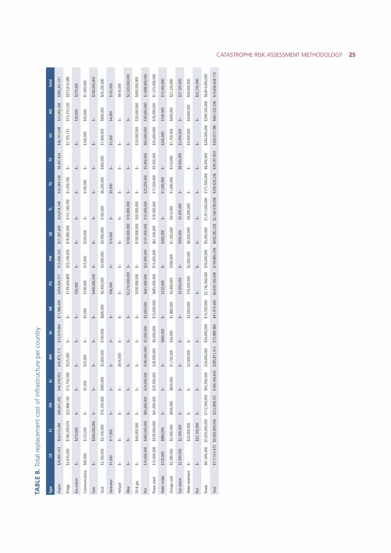
database. Significant infrastructure assets are typically built to higher standards than residential structures, and their quality is similar throughout the entire PIC re-gion. Therefore, our estimates of the unit replacement costs are independent of the location. An example of the unit replacement costs of infrastructure in the PICs is shown in Table 7 while the total replacement cost of the infrastructure for each country is shown in Table 8.
FIGURE 14. Location of major infrastructure assets in PG
Major Infrastructure
AIRPORT
HELIPAD
POWER PLANT
PORT
DOCK
DAM
MINE
OIL & GAS
COMMUNICATIONS
STORAGE TANK
GENERATOR
SUB-STATION
WATER TREATMENT
WATER INTAKE
BUS STATION
ROAD
BRIDGE
24 Pacific Catastrophe Risk Assessment and Financing Initiative (PCRAFI)
TABLE 7. Unit replacement costs of infrastructure in PIC
Type Cost (US$) Metric
Large Airport 518 per linear foot of runwayMedium Airport 366 per linear foot of runwayHelipad 88,000 per unit (40 12.5’-by-20’ slabs)Airstrip 10,000 per unitSmall Airport 100,000 per unitDam 100,000,000 per unitLarge Scale Mine 500,000,000 per unitMedium Scale Mine 100,000,000 per unitSmall Scale Mine 10,000,000 per unitSteel/Concrete Bridge 10,000 per linear meter of spanNon-Steel/Concrete Bridge 1,000 per linear meter of spanRoads 500,000 per linear kilometerRailroads 100,000 per linear kilometerDock 100,000 per unitWater Treatment 2,000,000 per unitStorage Tanks 10,000 per unitWater Intake 40,000 per unitBus Station 30,000 per unitCommunications 5,000 per unitOil & Gas Facility 20,000,000 per unitPower Plant - Very Large 40,000,000 per unitPower Plant - Large 10,000,000 per unitPower Plant - Medium 5,000,000 per unitPower Plant - Small 1,000,000 per unitPower Plant - Very Small 500,000 per unitGenerator 1,000 per unitSubstation 500,000 per unitPort - Very Large 100,000,000 per unitPort - Large 50,000,000 per unitPort - Medium 10,000,000 per unitPort - Small 5,000,000 per unitPort - Very Small 1,000,000 per unit
1.4 Crops
The crop exposure database is a comprehensive inventory of major cash crops – their location, types, and replacement costs. It does not directly consider subsistence crops or forestry. The spatial dis-tribution of major crops was derived from moderate-resolution satellite imagery and image detection tech-niques. To the extent possible, results were validated using high-resolution imagery, agricultural census data, ancillary data collected during the course of the project (FJ, TO and VU) and feedback from local experts.
The crop exposure database is a subset of a more comprehensive Land Use / Land Cover (LULC) geo-database, in which other land use categories were indexed (e.g., forests, lakes and rivers, sand, settlements, barren land, and grass land). The LULC maps were generated primarily using remote sensing and were supplemented with various sources. To our knowledge, this is the first time that LULC maps were derived and made available to the public for the PIC region. Similar to the identification of building locations in rural areas, the LULC maps were developed using satellite imagery (mostly moderate-
CATASTROPHE RISK ASSESSMENT METHODOLOGY 25
TAB
LE 8
. Tot
al r
epla
cem
ent
cost
of
infr
astr
uctu
re p
er c
ount
ry
Type
CKFJ
FMKI
MH
NI
NR
PGPW
SBTL
TOTV
VUW
STo
tal
Airp
ort
$20
,891
,472
$
54,0
13,0
80
$40
,641
,392
$
40,2
59,0
53
$43
,875
,113
$
13,0
19,9
60
$11
,988
,400
$
204,
069,
571
$12
,439
,320
$
21,5
87,6
00
$24
,818
,248
$
29,3
89,5
36
$8,
497,
824
$36
,707
,648
$
23,0
63,3
06
$58
5,26
1,52
1
Brid
ge $
2,91
0,00
0 $
180,
399,
974
$22
,968
,139
$
12,1
50,5
90
$52
5,30
0 $
–
$–
$
139,
044,
869
$23
,149
,939
$
18,9
90,9
26
$15
1,74
9,79
0 $
1,45
9,70
0 $
–
$7,
155,
132
$13
,310
,230
$
573,
814,
589
Bus
stat
ion
$–
$
210,
000
$–
$
–
$–
$
–
$–
$
30,0
00
$–
$
–
$–
$
–
$–
$
–
$30
,000
$
270,
000
Com
mun
icatio
ns $
60,0
00
$12
5,00
0 $
–
$5,
000
$25
,000
$
–
$5,
000
$19
0,00
0 $
15,0
00
$23
0,00
0 $
–
$14
0,00
0 $
–
$16
0,00
0 $
45,0
00
$1,
000,
000
Dam
$–
$
300,
000,
000
$–
$
–
$–
$
–
$–
$
400,
000,
000
$–
$
–
$–
$
–
$–
$
–
$–
$
700,
000,
000
Dock
$2,
700,
000
$3,
100,
000
$10
,100
,000
$
900,
000
$2,
600,
000
$10
0,00
0 $
600,
000
$6,
400,
000
$3,
900,
000
$3,
900,
000
$10
0,00
0 $
6,20
0,00
0 $
400,
000
$1,
600,
000
$60
0,00
0 $
43,2
00,0
00
Gen
erat
or $
1,00
0 $
17,0
00
$–
$
–
$–
$
–
$–
$
56,0
00
$–
$
14,0
00
$–
$
5,00
0 $
–
$5,
000
$4,
000
$10
2,00
0
Helip
ad $
–
$–
$
–
$–
$
616,
000
$–
$
–
$–
$
–
$–
$
–
$–
$
–
$–
$
–
$61
6,00
0
Min
e $
–
$–
$
–
$–
$
–
$–
$
–
$2,2
10,0
00,0
00
$–
$
100,
000,
000
$10
,000
,000
$
–
$–
$
–
$–
$
2,32
0,00
0,00
0
Oil
& ga
s $
–
$40
,000
,000
$
–
$–
$
–
$–
$
–
$20
0,00
0,00
0 $
–
$10
0,00
0,00
0 $
20,0
00,0
00
$–
$
–
$20
,000
,000
$
20,0
00,0
00
$40
0,00
0,00
0
Port
$10
,000
,000
$
482,
000,
000
$85
,000
,000
$
24,0
00,0
00
$18
2,00
0,00
0 $
1,00
0,00
0 $
5,00
0,00
0 $
641,
000,
000
$27
,000
,000
$
101,
000,
000
$15
,000
,000
$
25,0
00,0
00
$5,
000,
000
$65
,000
,000
$
30,0
00,0
00
$1,
698,
000,
000
Pow
er p
lant
$13
,500
,000
$
339,
000,
000
$41
,000
,000
$
20,5
00,0
00
$28
,500
,000
$
5,00
0,00
0 $
10,0
00,0
00
$68
5,00
0,00
0 $
15,0
00,0
00
$61
,500
,000
$
18,5
00,0
00
$17
,000
,000
$
9,50
0,00
0 $
35,0
00,0
00
$76
,000
,000
$
1,37
5,00
0,00
0
Wat
er in
take
$72
0,00
0 $
880,
000
$–
$
–
$–
$
840,
000
$–
$
320,
000
$–
$
360,
000
$–
$
7,04
0,00
0 $
–
$24
0,00
0 $
160,
000
$10
,560
,000
Stor
age
tank
$2,
290,
000
$4,
560,
000
$60
0,00
0 $
850,
000
$1,
730,
000
$30
,000
$
1,88
0,00
0 $
3,49
0,00
0 $
390,
000
$1,
200,
000
$41
0,00
0 $
1,69
0,00
0 $
310,
000
$1,
150,
000
$64
0,00
0 $
21,2
20,0
00
Sub-
stat
ion
$3,
500,
000
$2,
500,
000
$–
$
–
$–
$
–
$–
$
3,00
0,00
0 $
–
$50
0,00
0 $
5,00
0,00
0 $
–
$8,
000,
000
$5,
000,
000
$–
$
27,5
00,0
00
Wat
er tr
eatm
ent
$–
$
20,0
00,0
00
$–
$
–
$2,
000,
000
$–
$
2,00
0,00
0 $
10,0
00,0
00
$2,
000,
000
$6,
000,
000
$4,
000,
000
$–
$
–
$4,
000,
000
$4,
000,
000
$54
,000
,000
Rail
$–
$
32,1
00,0
00
$–
$
–
$–
$
–
$–
$
–
$–
$
–
$–
$
–
$–
$
–
$–
$
32,1
00,0
00
Road
s $
61,0
00,0
00
$1,6
35,0
00,0
00
$11
2,50
0,00
0 $
65,5
00,0
00
$24
,000
,000
$
54,0
00,0
00
$10
,500
,000
$2
,136
,500
,000
$
76,0
00,0
00
$5,
000,
000
$1,9
11,0
00,0
00
$17
1,50
0,00
0 $
8,00
0,00
0 $
244,
000,
000
$29
9,50
0,00
0 $
6,81
4,00
0,00
0
Tota
l $
117,
572,
472
$3,0
93,9
05,0
54
$31
2,80
9,53
1 $
164,
164,
643
$28
5,87
1,41
2 $
73,9
89,9
60
$41
,973
,400
$6
,639
,100
,440
$
159,
894,
259
$42
0,28
2,52
6 $2
,160
,578
,038
$
259,
424,
236
$39
,707
,824
$
420,
017,
780
$46
7,35
2,53
6 $
14,6
56,6
44,1
10
26 Pacific Catastrophe Risk Assessment and Financing Initiative (PCRAFI)
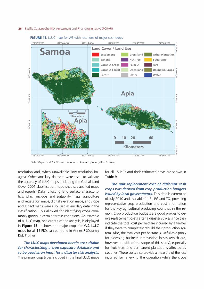
resolution and, when unavailable, low-resolution im-ages). Other ancillary datasets were used to validate the accuracy of LULC maps, including the Global Land Cover 2001 classification, topo-sheets, classified maps and reports. Data reflecting land surface characteris-tics, which include land suitability maps, agriculture and vegetation maps, digital elevation maps, and slope and aspect maps were also used as ancillary data in the classification. This allowed for identifying crops com-monly grown in certain terrain conditions. An example of a LULC map, one output of the analysis, is displayed in Figure 15. It shows the major crops for WS. LULC maps for all 15 PICs can be found in Annex F (Country Risk Profiles).
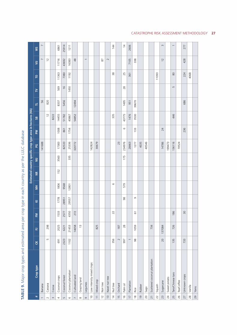
The LULC maps developed herein are suitable for characterizing a crop exposure database and to be used as an input for a disaster risk analysis. The primary crop types included in the final LULC maps
for all 15 PICs and their estimated areas are shown in Table 9.
The unit replacement cost of different cash crops was derived from crop production budgets issued by local governments. This data is current as of July 2010 and available for FJ, PG and TO, providing representative crop production and cost information for the key agricultural producing countries in the re-gion. Crop production budgets are good proxies to de-rive replacement costs after a disaster strikes since they indicate the total cost per hectare incurred by a farmer if they were to completely rebuild their production sys-tem. Also, the total cost per hectare is useful as a proxy for assessing business interruption losses (which are, however, outside of the scope of this study), especially for fruit trees and permanent plantations affected by cyclones. These costs also provide a measure of the loss incurred for renewing the operation while the crops
FIGURE 15. LULC map for WS with locations of major cash crops
Note: Maps for all 15 PICs can be found in Annex F (Country Risk Profiles)
CATASTROPHE RISK ASSESSMENT METHODOLOGY 27
TAB
LE 9
. Maj
or c
rop
type
s an
d es
timat
ed a
rea
per
crop
typ
e in
eac
h co
untr
y as
per
the
LU
LC d
atab
ase
#Cr
op t
ype
Esti
mat
ed c
ount
ry s
peci
fic c
rop
type
are
a in
hec
tare
s (H
A)
CKFJ
FMKI
MH
NR
NU
PGPW
SBTL
TVTO
VUW
S
1Ba
nana
1416
8856
77
2C
assa
va5
298
1282
012
3C
ocoa
8222
4C
ocon
ut c
rops
691
2025
1533
1778
1806
152
3560
1738
310
0814
455
8337
569
1136
311
716
6861
5C
ocon
ut f
ores
t23
2362
2125
7728
951
9568
8253
386
151
782
5456
1673
8043
692
2591
4
6C
ocon
ut p
lant
atio
n11
0221
453
4350
2955
712
801
335
2533
617
5440
867
1450
1192
1638
312
11
7C
ultiv
ated
land
1465
827
232
0772
5485
212
494
48
8G
razi
ng la
nd13
9Le
gum
es1
10Lo
w in
tens
ity m
ixed
cro
ps14
2824
11M
ixed
cro
p82
530
679
12N
ori t
ree
87
13N
avel
nut
tre
e2
14N
ut t
ree
356
226
335
3814
4
15O
rcha
rd2
187
23
16Pa
lm o
il99
728
9857
917
523
4976
643
775
1495
2825
14
17Pl
anta
tion
128
463
1476
951
361
7105
2606
18Ri
ce98
1059
619
1277
133
3530
3967
033
8
19Ru
bber
4035
20Sa
go40
546
21Sc
atte
red
coco
nut
plan
tatio
n73
4
22Sq
uash
1109
3
23Su
garc
ane
2013
7084
1478
624
123
24Sw
eet
pota
to19
9473
25Ta
ro/C
hine
se t
aro
135
726
186
1361
1644
65
801
26Te
a/C
offe
e70
524
27U
nkno
wn
crop
s73
330
236
686
224
428
277
28Va
nilla
4068
29Ya
ms
28 Pacific Catastrophe Risk Assessment and Financing Initiative (PCRAFI)
TABLE 10. Replacement costs for key crops under different production systems in the PICs
Crop type
Averagereplacement cost (US$ per hecatre)
Replacement cost subsistence
(US$ per hecatre)
Replacement cost commercial farmer(US$ per hecatre)
Banana 4,065 1,016 6,098
Breadfruit 386 97 579
Cassava 2,468 617 3,702
Cocoa 1,766 442 2,649
Coconut (Copra) 294 74 441
Coconut (Fresh Nut) 504 126 756
Coconut (Mature Nut) 504 126 756
Coffee 1,512 378 2,268
Ginger 7,697 1,924 11,546
Gourd/Squash 1,213 303 1,820
Kava/Yaqona 3,532 883 5,298
Lemon 966 242 1,449
Mango 375 94 563
Nut Tree 1,750 438 2,625
Oil Palm 5,300 1,325 7,950
Papaya 3,039 760 4,559
Pineapple 2,009 502 3,014
Pumpkin 2,999 750 4,499
Rubber Tree 504 126 756
Sago Palm 1,488 372 2,232
Sugarcane 1,234 309 1,851
Sweet Corn/Maize 1,822 456 2,733
Sweet Potato 1,474 369 2,211
Giant Taro/Ta’amu 1,365 341 2,048
Taro 2,993 748 4,490
Tobacco 9,080 2,270 13,620
Vanilla 1,243 311 1,865
Yam 9,843 2,461 14,765
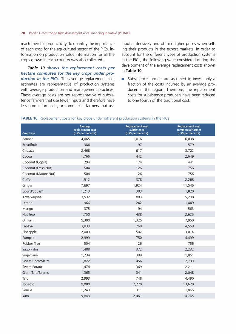
reach their full productivity. To quantify the importance of each crop for the agricultural sector of the PICs, in-formation on production value information for all the crops grown in each country was also collected.
Table 10 shows the replacement costs per hectare computed for the key crops under pro-duction in the PICs. The average replacement cost estimates are representative of production systems with average production and management practices. These average costs are not representative of subsis-tence farmers that use fewer inputs and therefore have less production costs, or commercial farmers that use
inputs intensively and obtain higher prices when sell-ing their products in the export markets. In order to account for the different types of production systems in the PICs, the following were considered during the development of the average replacement costs shown in Table 10:
�� Subsistence farmers are assumed to invest only a fraction of the costs incurred by an average pro-ducer in the region. Therefore, the replacement costs for subsistence producers have been reduced to one fourth of the traditional cost.
CATASTROPHE RISK ASSESSMENT METHODOLOGY 29
�� Commercial producers that invest heavily in tech-nology and whose production is oriented towards export markets are assumed to have higher re-placement costs than the average crop production systems. For commercial farmers, the replacement costs have been increased by half of the traditional cost.
For the purpose of the risk assessment, re-placement cost estimates used for cash crops are consistent with those for commercial farmers, which is appropriate when estimating the losses caused to cash crops by tropical cyclones. In addi-tion, the values in Table 10 were modified slightly to correspond with each country’s GDP for the agriculture sector as given in the CIA World Factbook. This final step ensures the validity and consistency of the total crop asset value for each country.
The LULC databases, which contain informa-tion on all vegetation, were used to create the cash crop exposure database. Cash crops were in-dexed by sampling the LULC data on an 80-by-80 me-ter grid for most countries. For the larger countries (PG, WS and FJ), the sampling grid was taken at 270 by 270 meters. These different sampling resolutions balanced accuracy and economy, allowing for the detection of cash crops in small atolls. In addition, the crop types
indicated in the LULC maps, which sometimes included multiple crops in one area, were mapped appropriately to a similar crop classification in which the replacement costs (see later in this section) and damage functions could be easily assigned.
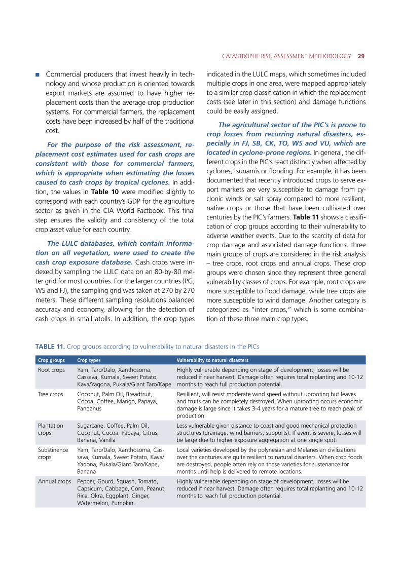
The agricultural sector of the PIC’s is prone to crop losses from recurring natural disasters, es-pecially in FJ, SB, CK, TO, WS and VU, which are located in cyclone-prone regions. In general, the dif-ferent crops in the PIC’s react distinctly when affected by cyclones, tsunamis or flooding. For example, it has been documented that recently introduced crops to serve ex-port markets are very susceptible to damage from cy-clonic winds or salt spray compared to more resilient, native crops or those that have been cultivated over centuries by the PIC’s farmers. Table 11 shows a classifi-cation of crop groups according to their vulnerability to adverse weather events. Due to the scarcity of data for crop damage and associated damage functions, three main groups of crops are considered in the risk analysis – tree crops, root crops and annual crops. These crop groups were chosen since they represent three general vulnerability classes of crops. For example, root crops are more susceptible to flood damage, while tree crops are more susceptible to wind damage. Another category is categorized as “inter crops,” which is some combina-tion of these three main crop types.
Crop groups Crop types Vulnerability to natural disasters
Root crops Yam, Taro/Dalo, Xanthosoma, Cassava, Kumala, Sweet Potato, Kava/Yaqona, Pukala/Giant Taro/Kape
Highly vulnerable depending on stage of development, losses will be reduced if near harvest. Damage often requires total replanting and 10-12 months to reach full production potential.
Tree crops Coconut, Palm Oil, Breadfruit, Cocoa, Coffee, Mango, Papaya, Pandanus
Resillient, will resist moderate wind speed without uprooting but leaves and fruits can be completely destroyed. When uprooting occurs economic damage is large since it takes 3-4 years for a mature tree to reach peak of production.
Plantation crops
Sugarcane, Coffee, Palm Oil, Coconut, Cocoa, Papaya, Citrus, Banana, Vanilla
Less vulnerable given distance to coast and good mechanical protection structures (drainage, wind barriers, supports). If event is severe, losses will be large due to higher exposure aggregation at one single spot.
Substinence crops
Yam, Taro/Dalo, Xanthosoma, Cas-sava, Kumala, Sweet Potato, Kava/Yaqona, Pukala/Giant Taro/Kape, Banana
Local varieties developed by the polynesian and Melanesian civilizations over the centuries are quite resilient to natural disasters. When crop foods are destroyed, people often rely on these varieties for sustenance for months until help is delivered to remote locations.
Annual crops Pepper, Gourd, Squash, Tomato, Capsicum, Cabbage, Corn, Peanut, Rice, Okra, Eggplant, Ginger, Watermelon, Pumpkin.
Highly vulnerable depending on stage of development, losses will be reduced if near harvest. Damage often requires total replanting and 10-12 months to reach full production potential.
TABLE 11. Crop groups according to vulnerability to natural disasters in the PICs
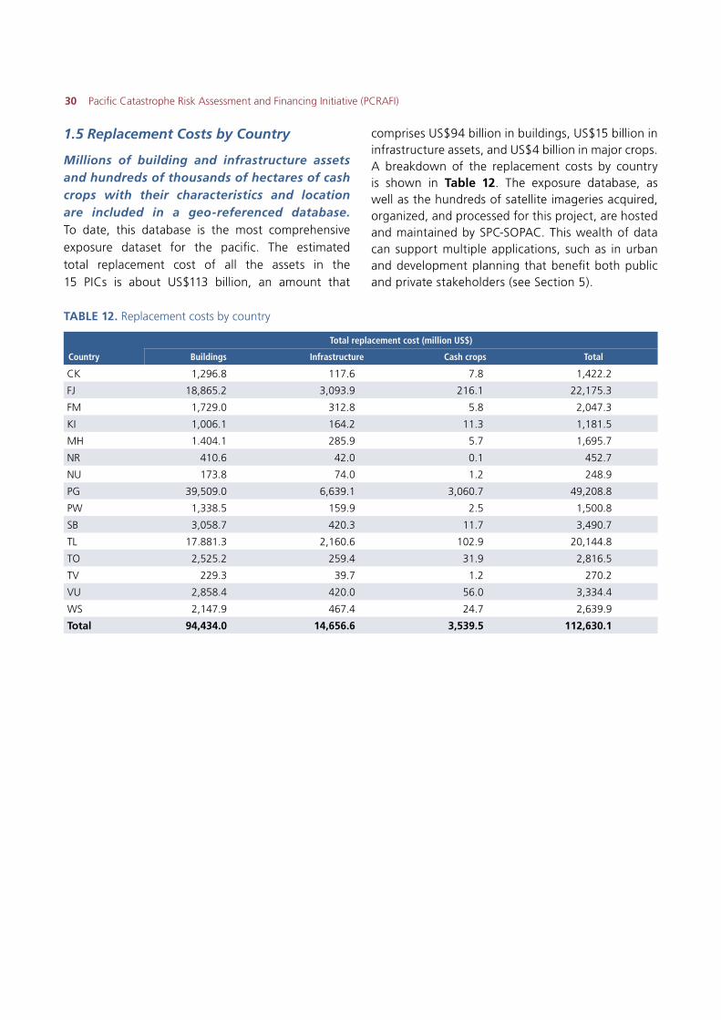
30 Pacific Catastrophe Risk Assessment and Financing Initiative (PCRAFI)
1.5 Replacement Costs by Country
Millions of building and infrastructure assets and hundreds of thousands of hectares of cash crops with their characteristics and location are included in a geo-referenced database. To date, this database is the most comprehensive exposure dataset for the pacific. The estimated total replacement cost of all the assets in the 15 PICs is about US$113 billion, an amount that
comprises US$94 billion in buildings, US$15 billion in infrastructure assets, and US$4 billion in major crops. A breakdown of the replacement costs by country is shown in Table 12. The exposure database, as well as the hundreds of satellite imageries acquired, organized, and processed for this project, are hosted and maintained by SPC-SOPAC. This wealth of data can support multiple applications, such as in urban and development planning that benefit both public and private stakeholders (see Section 5).
Country
Total replacement cost (million US$)
Buildings Infrastructure Cash crops Total
CK 1,296.8 117.6 7.8 1,422.2
FJ 18,865.2 3,093.9 216.1 22,175.3
FM 1,729.0 312.8 5.8 2,047.3
KI 1,006.1 164.2 11.3 1,181.5
MH 1.404.1 285.9 5.7 1,695.7
NR 410.6 42.0 0.1 452.7
NU 173.8 74.0 1.2 248.9
PG 39,509.0 6,639.1 3,060.7 49,208.8
PW 1,338.5 159.9 2.5 1,500.8
SB 3,058.7 420.3 11.7 3,490.7
TL 17.881.3 2,160.6 102.9 20,144.8
TO 2,525.2 259.4 31.9 2,816.5
TV 229.3 39.7 1.2 270.2
VU 2,858.4 420.0 56.0 3,334.4
WS 2,147.9 467.4 24.7 2,639.9
Total 94,434.0 14,656.6 3,539.5 112,630.1
TABLE 12. Replacement costs by country
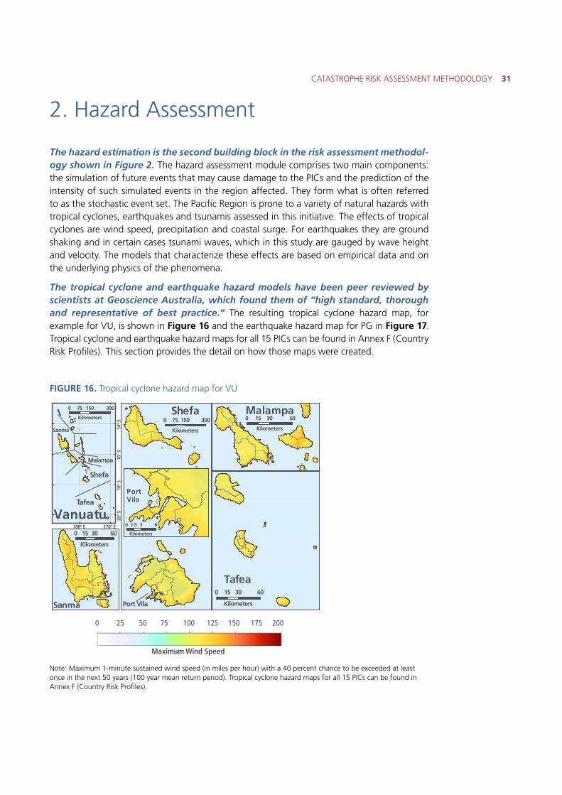
CATASTROPHE RISK ASSESSMENT METHODOLOGY 31
2. Hazard Assessment
The hazard estimation is the second building block in the risk assessment methodol-ogy shown in Figure 2. The hazard assessment module comprises two main components: the simulation of future events that may cause damage to the PICs and the prediction of the intensity of such simulated events in the region affected. They form what is often referred to as the stochastic event set. The Pacific Region is prone to a variety of natural hazards with tropical cyclones, earthquakes and tsunamis assessed in this initiative. The effects of tropical cyclones are wind speed, precipitation and coastal surge. For earthquakes they are ground shaking and in certain cases tsunami waves, which in this study are gauged by wave height and velocity. The models that characterize these effects are based on empirical data and on the underlying physics of the phenomena.
The tropical cyclone and earthquake hazard models have been peer reviewed by scientists at Geoscience Australia, which found them of “high standard, thorough and representative of best practice.” The resulting tropical cyclone hazard map, for example for VU, is shown in Figure 16 and the earthquake hazard map for PG in Figure 17. Tropical cyclone and earthquake hazard maps for all 15 PICs can be found in Annex F (Country Risk Profiles). This section provides the detail on how those maps were created.
FIGURE 16. Tropical cyclone hazard map for VU
Note: Maximum 1-minute sustained wind speed (in miles per hour) with a 40 percent chance to be exceeded at least once in the next 50 years (100 year mean return period). Tropical cyclone hazard maps for all 15 PICs can be found in Annex F (Country Risk Profiles).
170° E168° E
14° S
16° S
18° S
20° S
Tafea
MalampaShefa
Vanuatu0 30 6015
Kilometers
0 150 30075
Kilometers 0 150 30075
Kilometers
0 30 6015
Kilometers
0 30 6015
Kilometers
Sanma Port Vila
Shefa
Malampa
Tafea
Sanma
PortVila
0 3 61.5
Kilometers
0 25 50 75 100 125 150 175 200
Maximum Wind Speed
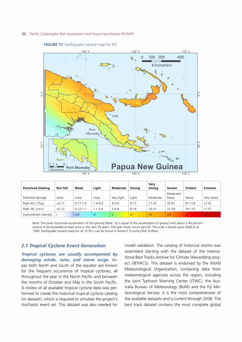
32 Pacific Catastrophe Risk Assessment and Financing Initiative (PCRAFI)
FIGURE 17. Earthquake hazard map for PG
Note: The peak horizontal acceleration of the ground (Note: 1g is equal to the acceleration of gravity) with about a 40 percent chance to be exceeded at least once in the next 50 years (100-year mean return period). The scale is based upon Wald et al. 1999. Earthquake hazard maps for all 15 PICs can be found in Annex F (Country Risk Profiles).
2.1 Tropical Cyclone Event Generation
Tropical cyclones are usually accompanied by damaging winds, rains, and storm surge. Ar-eas both North and South of the equator are known for the frequent occurrence of tropical cyclones, all throughout the year in the North Pacific and between the months of October and May in the South Pacific. A review of all available tropical cyclone data was per-formed to create the historical tropical cyclone catalog (or dataset), which is required to simulate the project’s stochastic event set. This dataset was also needed for
model validation. The catalog of historical storms was assembled starting with the dataset of the Interna-tional Best Tracks Archive for Climate Stewardship proj-ect (IBTrACS). This dataset is endorsed by the World Meteorological Organization, containing data from meteorological agencies across the region, including the Joint Typhoon Warning Center (JTWC), the Aus-tralia Bureau of Meteorology (BoM) and the Fiji Me-teorological Service. It is the most comprehensive of the available datasets and is current through 2008. The best track dataset contains the most complete global
Perceived shaking Not felt Weak Light Moderate StrongVery strong Severe Violent Extreme
Potential damage none none none Very light Light ModerateModerate/heavy Heavy Very heavy
Peak ACC (%g) <0.17 0.17-1.4 1.4-4.0 4.0-9 9-17 17-32 32-61 61-114 >114
Peak Vel. (cm’s) <0.12 0.12-1.1 1.1-3.4 3.4-8 8-16 16-31 31-59 59-115 >115
Instrumental intensity I II-III IV V VI VII VIII IX X+
PortMoresby
Lae
155° E
155° E
150° E
150° E
145° E
145° E
5° S
5° S
10°
S
10°
S
Papua New Guinea
0 200 400100
Kilometers
0 6 123
Kilometers Port Moresby
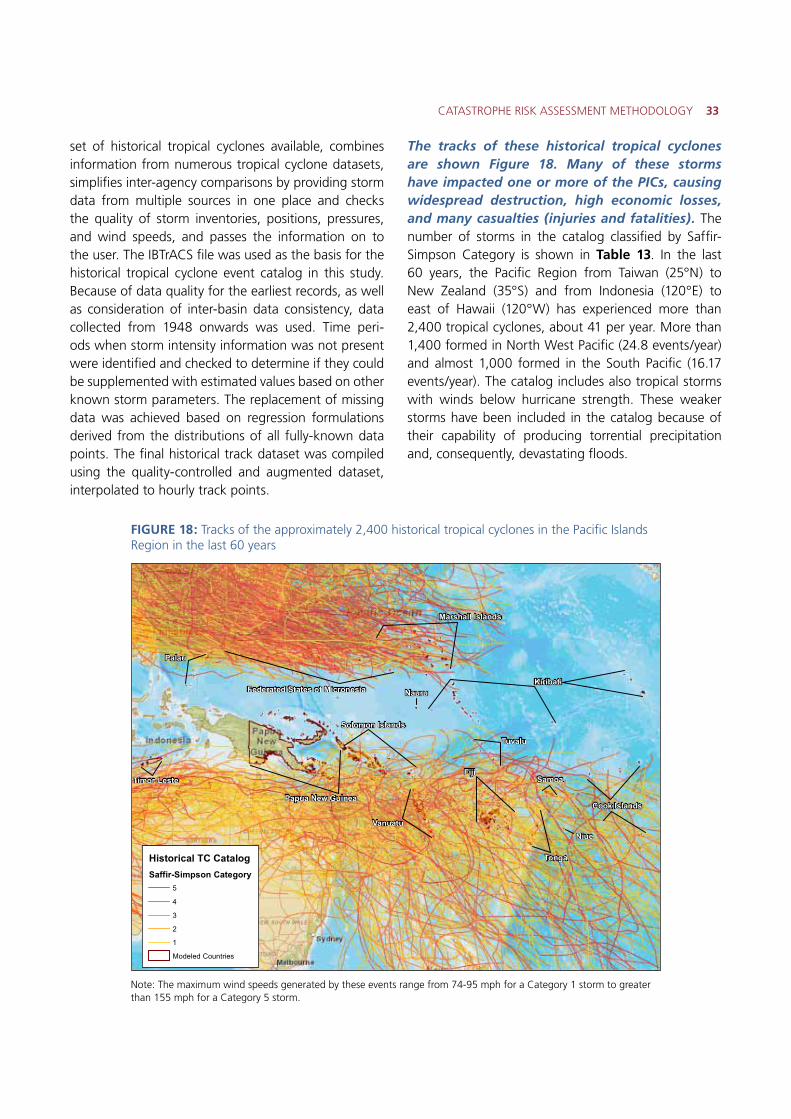
CATASTROPHE RISK ASSESSMENT METHODOLOGY 33
set of historical tropical cyclones available, combines information from numerous tropical cyclone datasets, simplifies inter-agency comparisons by providing storm data from multiple sources in one place and checks the quality of storm inventories, positions, pressures, and wind speeds, and passes the information on to the user. The IBTrACS file was used as the basis for the historical tropical cyclone event catalog in this study. Because of data quality for the earliest records, as well as consideration of inter-basin data consistency, data collected from 1948 onwards was used. Time peri-ods when storm intensity information was not present were identified and checked to determine if they could be supplemented with estimated values based on other known storm parameters. The replacement of missing data was achieved based on regression formulations derived from the distributions of all fully-known data points. The final historical track dataset was compiled using the quality-controlled and augmented dataset, interpolated to hourly track points.
The tracks of these historical tropical cyclones are shown Figure 18. Many of these storms have impacted one or more of the PICs, causing widespread destruction, high economic losses, and many casualties (injuries and fatalities). The number of storms in the catalog classified by Saffir-Simpson Category is shown in Table 13. In the last 60 years, the Pacific Region from Taiwan (25°N) to New Zealand (35°S) and from Indonesia (120°E) to east of Hawaii (120°W) has experienced more than 2,400 tropical cyclones, about 41 per year. More than 1,400 formed in North West Pacific (24.8 events/year) and almost 1,000 formed in the South Pacific (16.17 events/year). The catalog includes also tropical storms with winds below hurricane strength. These weaker storms have been included in the catalog because of their capability of producing torrential precipitation and, consequently, devastating floods.
Marshall Islands
Federated States of Micronesia
Palau
Timor-Leste
Papua New Guinea
Vanuatu
Tonga
Niue
Solomon Islands
Kiribati
Tuvalu
FijiSamoa
Cook Islands
Nauru
Historical TC CatalogSaffir-Simpson Category
5
4
3
2
1
Modeled Countries
FIGURE 18: Tracks of the approximately 2,400 historical tropical cyclones in the Pacific Islands Region in the last 60 years
Note: The maximum wind speeds generated by these events range from 74-95 mph for a Category 1 storm to greater than 155 mph for a Category 5 storm.
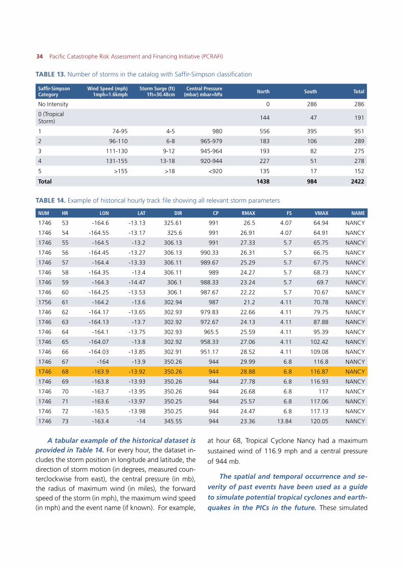
34 Pacific Catastrophe Risk Assessment and Financing Initiative (PCRAFI)
TABLE 13. Number of storms in the catalog with Saffir-Simpson classification
Saffir-Simpson Category
Wind Speed (mph) 1mph=1.6kmph
Storm Surge (ft) 1ft=30.48cm
Central Pressure (mbar) mbar=hPa North South Total
No Intensity 0 286 286
0 (Tropical Storm)
144 47 191
1 74-95 4-5 980 556 395 951
2 96-110 6-8 965-979 183 106 289
3 111-130 9-12 945-964 193 82 275
4 131-155 13-18 920-944 227 51 278
5 >155 >18 <920 135 17 152
Total 1438 984 2422
NUM HR LON LAT DIR CP RMAX FS VMAX NAME
1746 53 -164.6 -13.13 325.61 991 26.5 4.07 64.94 NANCY
1746 54 -164.55 -13.17 325.6 991 26.91 4.07 64.91 NANCY
1746 55 -164.5 -13.2 306.13 991 27.33 5.7 65.75 NANCY
1746 56 -164.45 -13.27 306.13 990.33 26.31 5.7 66.75 NANCY
1746 57 -164.4 -13.33 306.11 989.67 25.29 5.7 67.75 NANCY
1746 58 -164.35 -13.4 306.11 989 24.27 5.7 68.73 NANCY
1746 59 -164.3 -14.47 306.1 988.33 23.24 5.7 69.7 NANCY
1746 60 -164.25 -13.53 306.1 987.67 22.22 5.7 70.67 NANCY
1756 61 -164.2 -13.6 302.94 987 21.2 4.11 70.78 NANCY
1746 62 -164.17 -13.65 302.93 979.83 22.66 4.11 79.75 NANCY
1746 63 -164.13 -13.7 302.92 972.67 24.13 4.11 87.88 NANCY
1746 64 -164.1 -13.75 302.93 965.5 25.59 4.11 95.39 NANCY
1746 65 -164.07 -13.8 302.92 958.33 27.06 4.11 102.42 NANCY
1746 66 -164.03 -13.85 302.91 951.17 28.52 4.11 109.08 NANCY
1746 67 -164 -13.9 350.26 944 29.99 6.8 116.8 NANCY
1746 68 -163.9 -13.92 350.26 944 28.88 6.8 116.87 NANCY
1746 69 -163.8 -13.93 350.26 944 27.78 6.8 116.93 NANCY
1746 70 -163.7 -13.95 350.26 944 26.68 6.8 117 NANCY
1746 71 -163.6 -13.97 350.25 944 25.57 6.8 117.06 NANCY
1746 72 -163.5 -13.98 350.25 944 24.47 6.8 117.13 NANCY
1746 73 -163.4 -14 345.55 944 23.36 13.84 120.05 NANCY
TABLE 14. Example of historical hourly track file showing all relevant storm parameters
A tabular example of the historical dataset is provided in Table 14. For every hour, the dataset in-cludes the storm position in longitude and latitude, the direction of storm motion (in degrees, measured coun-terclockwise from east), the central pressure (in mb), the radius of maximum wind (in miles), the forward speed of the storm (in mph), the maximum wind speed (in mph) and the event name (if known). For example,
at hour 68, Tropical Cyclone Nancy had a maximum
sustained wind of 116.9 mph and a central pressure
of 944 mb.
The spatial and temporal occurrence and se-
verity of past events have been used as a guide
to simulate potential tropical cyclones and earth-
quakes in the PICs in the future. These simulated
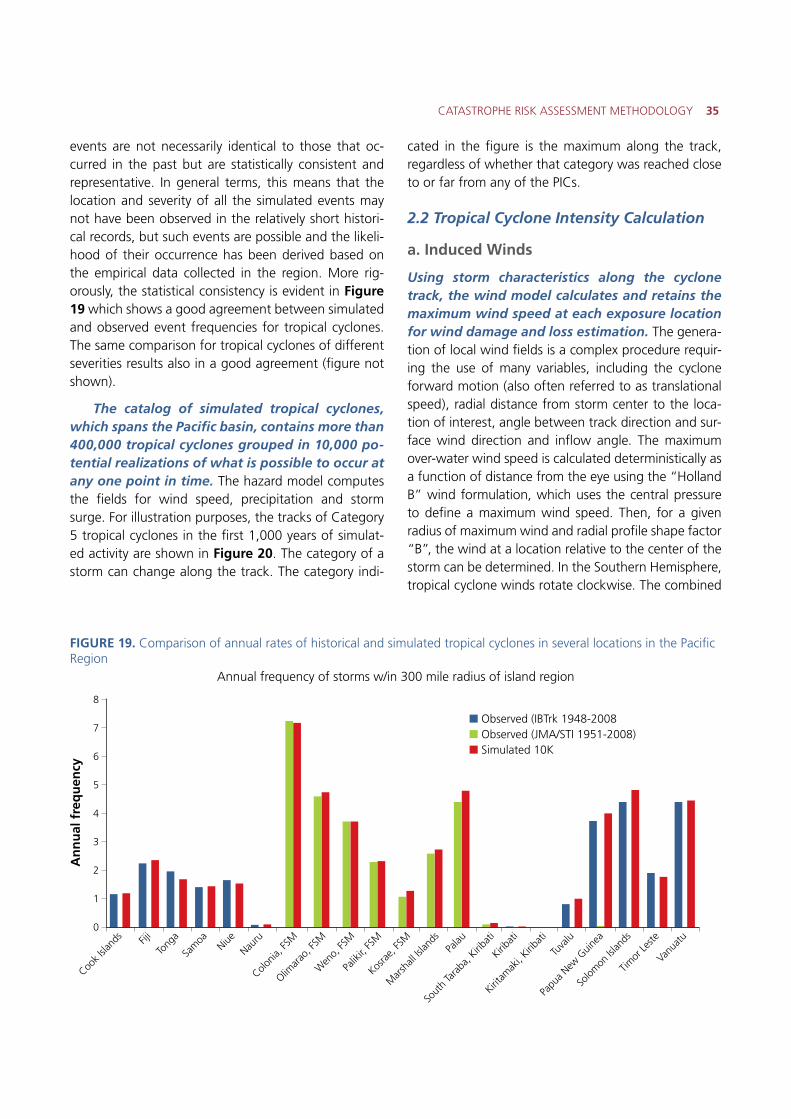
CATASTROPHE RISK ASSESSMENT METHODOLOGY 35
events are not necessarily identical to those that oc-curred in the past but are statistically consistent and representative. In general terms, this means that the location and severity of all the simulated events may not have been observed in the relatively short histori-cal records, but such events are possible and the likeli-hood of their occurrence has been derived based on the empirical data collected in the region. More rig-orously, the statistical consistency is evident in Figure 19 which shows a good agreement between simulated and observed event frequencies for tropical cyclones. The same comparison for tropical cyclones of different severities results also in a good agreement (figure not shown).
The catalog of simulated tropical cyclones, which spans the Pacific basin, contains more than 400,000 tropical cyclones grouped in 10,000 po-tential realizations of what is possible to occur at any one point in time. The hazard model computes the fields for wind speed, precipitation and storm surge. For illustration purposes, the tracks of Category 5 tropical cyclones in the first 1,000 years of simulat-ed activity are shown in Figure 20. The category of a storm can change along the track. The category indi-
cated in the figure is the maximum along the track, regardless of whether that category was reached close to or far from any of the PICs.
2.2 Tropical Cyclone Intensity Calculation
a. Induced Winds
Using storm characteristics along the cyclone track, the wind model calculates and retains the maximum wind speed at each exposure location for wind damage and loss estimation. The genera-tion of local wind fields is a complex procedure requir-ing the use of many variables, including the cyclone forward motion (also often referred to as translational speed), radial distance from storm center to the loca-tion of interest, angle between track direction and sur-face wind direction and inflow angle. The maximum over-water wind speed is calculated deterministically as a function of distance from the eye using the “Holland B” wind formulation, which uses the central pressure to define a maximum wind speed. Then, for a given radius of maximum wind and radial profile shape factor “B”, the wind at a location relative to the center of the storm can be determined. In the Southern Hemisphere, tropical cyclone winds rotate clockwise. The combined
Cook I
sland
s Fiji
Tong
a
Sam
oaNiue
Colonia
, FSM
Olimar
ao, F
SM
Wen
o, FS
M
Palik
ir, FS
M
Kosra
e, FS
M
Mar
shall
Islan
dsPa
lau
Sout
h Ta
raba
, Kirib
ati
Nauru
Kiribat
i
Tuva
lu
Solom
on Is
lands
Timor
Leste
Vanu
atu
Papu
a New
Guin
ea
Kiritam
aki, K
iribat
i
� Observed (IBTrk 1948-2008� Observed (JMA/STI 1951-2008)� Simulated 10K
Annual frequency of storms w/in 300 mile radius of island region
An
nu
al f
req
uen
cy
8
7
6
5
4
3
2
1
0
FIGURE 19. Comparison of annual rates of historical and simulated tropical cyclones in several locations in the Pacific Region
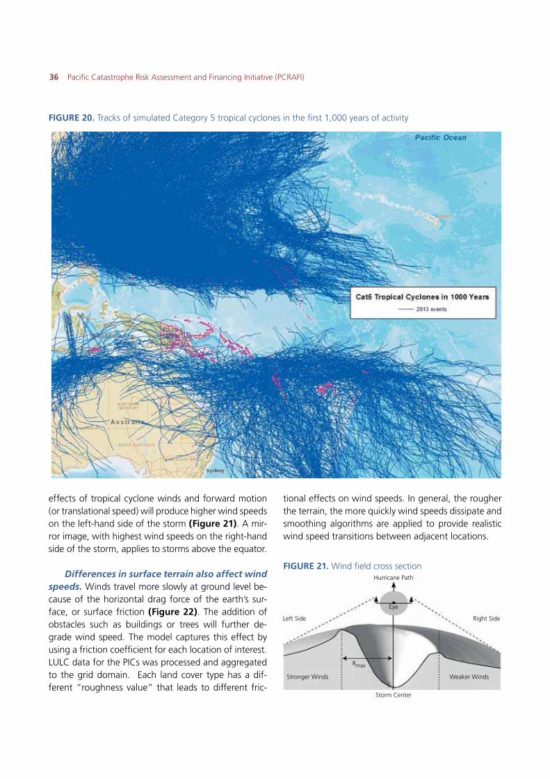
36 Pacific Catastrophe Risk Assessment and Financing Initiative (PCRAFI)
effects of tropical cyclone winds and forward motion (or translational speed) will produce higher wind speeds on the left-hand side of the storm (Figure 21). A mir-ror image, with highest wind speeds on the right-hand side of the storm, applies to storms above the equator.
Differences in surface terrain also affect wind speeds. Winds travel more slowly at ground level be-cause of the horizontal drag force of the earth’s sur-face, or surface friction (Figure 22). The addition of obstacles such as buildings or trees will further de-grade wind speed. The model captures this effect by using a friction coefficient for each location of interest. LULC data for the PICs was processed and aggregated to the grid domain. Each land cover type has a dif-ferent “roughness value” that leads to different fric-
tional effects on wind speeds. In general, the rougher the terrain, the more quickly wind speeds dissipate and smoothing algorithms are applied to provide realistic wind speed transitions between adjacent locations.
FIGURE 21. Wind field cross section
FIGURE 20. Tracks of simulated Category 5 tropical cyclones in the first 1,000 years of activity
Hurricane Path
Storm Center
Rmax
Eye
Right SideLeft Side
Weaker WindsStronger Winds
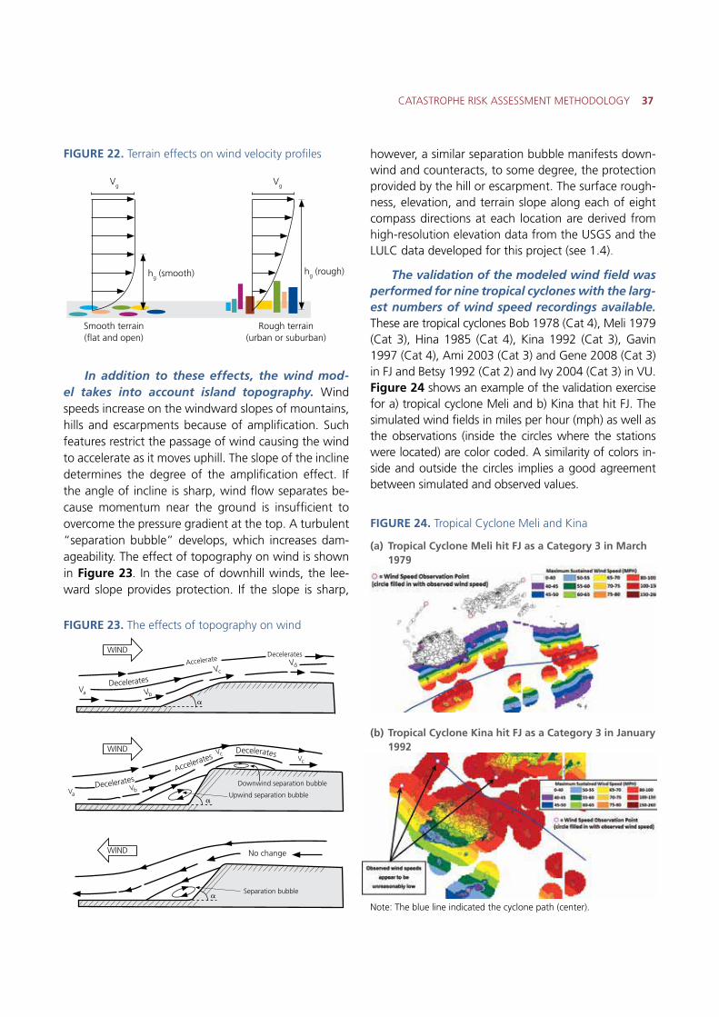
CATASTROPHE RISK ASSESSMENT METHODOLOGY 37
FIGURE 22. Terrain effects on wind velocity profiles
In addition to these effects, the wind mod-el takes into account island topography. Wind speeds increase on the windward slopes of mountains, hills and escarpments because of amplification. Such features restrict the passage of wind causing the wind to accelerate as it moves uphill. The slope of the incline determines the degree of the amplification effect. If the angle of incline is sharp, wind flow separates be-cause momentum near the ground is insufficient to overcome the pressure gradient at the top. A turbulent “separation bubble” develops, which increases dam-ageability. The effect of topography on wind is shown in Figure 23. In the case of downhill winds, the lee-ward slope provides protection. If the slope is sharp,
however, a similar separation bubble manifests down-wind and counteracts, to some degree, the protection provided by the hill or escarpment. The surface rough-ness, elevation, and terrain slope along each of eight compass directions at each location are derived from high-resolution elevation data from the USGS and the LULC data developed for this project (see 1.4).
The validation of the modeled wind field was performed for nine tropical cyclones with the larg-est numbers of wind speed recordings available. These are tropical cyclones Bob 1978 (Cat 4), Meli 1979 (Cat 3), Hina 1985 (Cat 4), Kina 1992 (Cat 3), Gavin 1997 (Cat 4), Ami 2003 (Cat 3) and Gene 2008 (Cat 3) in FJ and Betsy 1992 (Cat 2) and Ivy 2004 (Cat 3) in VU. Figure 24 shows an example of the validation exercise for a) tropical cyclone Meli and b) Kina that hit FJ. The simulated wind fields in miles per hour (mph) as well as the observations (inside the circles where the stations were located) are color coded. A similarity of colors in-side and outside the circles implies a good agreement between simulated and observed values.
FIGURE 24. Tropical Cyclone Meli and Kina
(a) Tropical Cyclone Meli hit FJ as a Category 3 in March 1979
(b) Tropical Cyclone Kina hit FJ as a Category 3 in January
1992
Note: The blue line indicated the cyclone path (center).
FIGURE 23. The effects of topography on wind
Smooth terrain(flat and open)
Vg
Rough terrain(urban or suburban)
Vg
hg (smooth) hg (rough)
Decelerates
Decelerates
DeceleratesAccelerate
Vb
Vb
Vc
VcVc
Vd
Va
Va
�
Decelerates
Accelerates
Downwind separation bubble
Upwind separation bubble
WIND
WIND
WIND
�
�
No change
Separation bubble
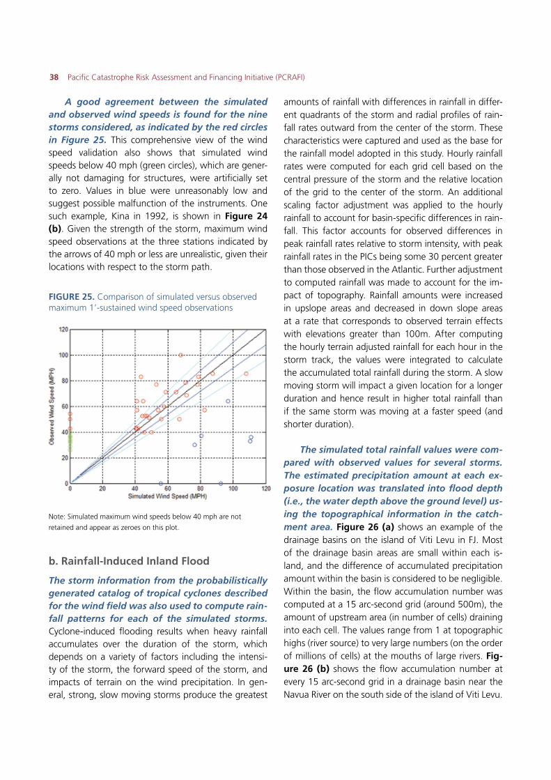
38 Pacific Catastrophe Risk Assessment and Financing Initiative (PCRAFI)
A good agreement between the simulated and observed wind speeds is found for the nine storms considered, as indicated by the red circles in Figure 25. This comprehensive view of the wind speed validation also shows that simulated wind speeds below 40 mph (green circles), which are gener-ally not damaging for structures, were artificially set to zero. Values in blue were unreasonably low and suggest possible malfunction of the instruments. One such example, Kina in 1992, is shown in Figure 24 (b). Given the strength of the storm, maximum wind speed observations at the three stations indicated by the arrows of 40 mph or less are unrealistic, given their locations with respect to the storm path.
FIGURE 25. Comparison of simulated versus observed maximum 1’-sustained wind speed observations
Note: Simulated maximum wind speeds below 40 mph are not
retained and appear as zeroes on this plot.
b. Rainfall-Induced Inland Flood
The storm information from the probabilistically generated catalog of tropical cyclones described for the wind field was also used to compute rain-fall patterns for each of the simulated storms. Cyclone-induced flooding results when heavy rainfall accumulates over the duration of the storm, which depends on a variety of factors including the intensi-ty of the storm, the forward speed of the storm, and impacts of terrain on the wind precipitation. In gen-eral, strong, slow moving storms produce the greatest
amounts of rainfall with differences in rainfall in differ-ent quadrants of the storm and radial profiles of rain-fall rates outward from the center of the storm. These characteristics were captured and used as the base for the rainfall model adopted in this study. Hourly rainfall rates were computed for each grid cell based on the central pressure of the storm and the relative location of the grid to the center of the storm. An additional scaling factor adjustment was applied to the hourly rainfall to account for basin-specific differences in rain-fall. This factor accounts for observed differences in peak rainfall rates relative to storm intensity, with peak rainfall rates in the PICs being some 30 percent greater than those observed in the Atlantic. Further adjustment to computed rainfall was made to account for the im-pact of topography. Rainfall amounts were increased in upslope areas and decreased in down slope areas at a rate that corresponds to observed terrain effects with elevations greater than 100m. After computing the hourly terrain adjusted rainfall for each hour in the storm track, the values were integrated to calculate the accumulated total rainfall during the storm. A slow moving storm will impact a given location for a longer duration and hence result in higher total rainfall than if the same storm was moving at a faster speed (and shorter duration).
The simulated total rainfall values were com-pared with observed values for several storms. The estimated precipitation amount at each ex-posure location was translated into flood depth (i.e., the water depth above the ground level) us-ing the topographical information in the catch-ment area. Figure 26 (a) shows an example of the drainage basins on the island of Viti Levu in FJ. Most of the drainage basin areas are small within each is-land, and the difference of accumulated precipitation amount within the basin is considered to be negligible. Within the basin, the flow accumulation number was computed at a 15 arc-second grid (around 500m), the amount of upstream area (in number of cells) draining into each cell. The values range from 1 at topographic highs (river source) to very large numbers (on the order of millions of cells) at the mouths of large rivers. Fig-ure 26 (b) shows the flow accumulation number at every 15 arc-second grid in a drainage basin near the Navua River on the south side of the island of Viti Levu.
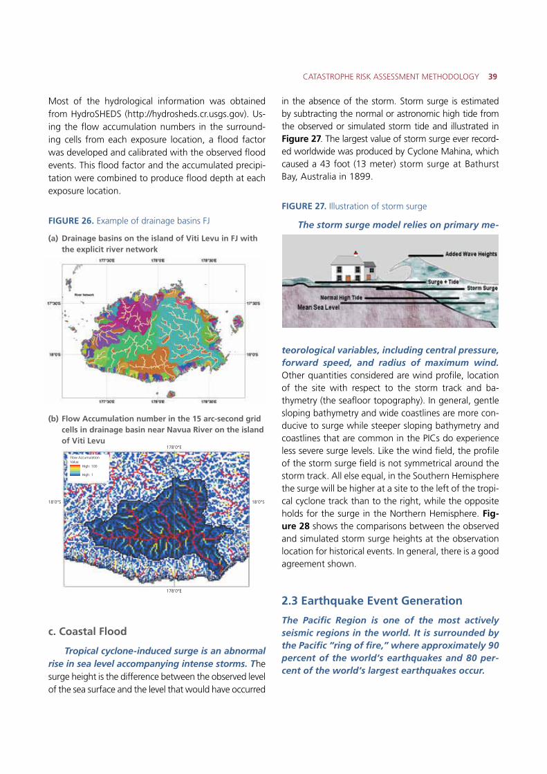
CATASTROPHE RISK ASSESSMENT METHODOLOGY 39
Most of the hydrological information was obtained from HydroSHEDS (http://hydrosheds.cr.usgs.gov). Us-ing the flow accumulation numbers in the surround-ing cells from each exposure location, a flood factor was developed and calibrated with the observed flood events. This flood factor and the accumulated precipi-tation were combined to produce flood depth at each exposure location.
FIGURE 26. Example of drainage basins FJ
(a) Drainage basins on the island of Viti Levu in FJ with the explicit river network
(b) Flow Accumulation number in the 15 arc-second grid cells in drainage basin near Navua River on the island of Viti Levu
c. Coastal Flood
Tropical cyclone-induced surge is an abnormal rise in sea level accompanying intense storms. The surge height is the difference between the observed level of the sea surface and the level that would have occurred
in the absence of the storm. Storm surge is estimated by subtracting the normal or astronomic high tide from the observed or simulated storm tide and illustrated in Figure 27. The largest value of storm surge ever record-ed worldwide was produced by Cyclone Mahina, which caused a 43 foot (13 meter) storm surge at Bathurst Bay, Australia in 1899.
FIGURE 27. Illustration of storm surge
The storm surge model relies on primary me-
teorological variables, including central pressure, forward speed, and radius of maximum wind. Other quantities considered are wind profile, location of the site with respect to the storm track and ba-thymetry (the seafloor topography). In general, gentle sloping bathymetry and wide coastlines are more con-ducive to surge while steeper sloping bathymetry and coastlines that are common in the PICs do experience less severe surge levels. Like the wind field, the profile of the storm surge field is not symmetrical around the storm track. All else equal, in the Southern Hemisphere the surge will be higher at a site to the left of the tropi-cal cyclone track than to the right, while the opposite holds for the surge in the Northern Hemisphere. Fig-ure 28 shows the comparisons between the observed and simulated storm surge heights at the observation location for historical events. In general, there is a good agreement shown.
2.3 Earthquake Event Generation
The Pacific Region is one of the most actively seismic regions in the world. It is surrounded by the Pacific “ring of fire,” where approximately 90 percent of the world’s earthquakes and 80 per-cent of the world’s largest earthquakes occur.
Flow AccumulationValue
High: 100
18’0°S 18’0°S
178’0°E
178’0°E
High: 1
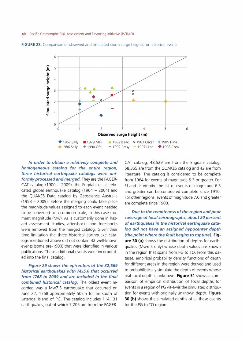
40 Pacific Catastrophe Risk Assessment and Financing Initiative (PCRAFI)
In order to obtain a relatively complete and homogeneous catalog for the entire region, three historical earthquake catalogs were uni-formly processed and merged. They are the PAGER-CAT catalog (1900 – 2009), the Engdahl et al. relo-cated global earthquake catalog (1964 – 2004) and the QUAKES Data catalog by Geoscience Australia (1958 – 2009). Before the merging could take place the magnitude values assigned to each event needed to be converted to a common scale, in this case mo-ment magnitude (Mw). As is customarily done in haz-ard assessment studies, aftershocks and foreshocks were removed from the merged catalog. Given their time limitation the three historical earthquake cata-logs mentioned above did not contain 42 well-known events (some pre-1900) that were identified in various publications. These additional events were incorporat-ed into the final catalog.
Figure 29 shows the epicenters of the 32,569 historical earthquakes with M�5.0 that occurred from 1768 to 2009 and are included in the final combined historical catalog. The oldest event re-corded was a Mw7.5 earthquake that occurred on June 22, 1768 approximately 50km to the south of Latangai Island of PG. The catalog includes 114,131 earthquakes, out of which 7,205 are from the PAGER-
CAT catalog, 48,529 are from the Engdahl catalog, 58,355 are from the QUAKES catalog and 42 are from literature. The catalog is considered to be complete from 1964 for events of magnitude 5.3 or greater. For FJ and its vicinity, the list of events of magnitude 6.5 and greater can be considered complete since 1910. For other regions, events of magnitude 7.0 and greater are complete since 1900.
Due to the remoteness of the region and poor coverage of local seismographs, about 20 percent of earthquakes in the historical earthquake cata-log did not have an assigned hypocenter depth (the point where the fault begins to rupture). Fig-ure 30 (a) shows the distribution of depths for earth-quakes (Mw� 5 only) whose depth values are known in the region that spans from PG to TO. From this da-taset, empirical probability density functions of depth for different areas in the region were derived and used to probabilistically simulate the depth of events whose real focal depth is unknown. Figure 31 shows a com-parison of empirical distribution of focal depths for events in a region of PG vis-à-vis the simulated distribu-tion for events with originally unknown depth. Figure 30 (b) shows the simulated depths of all these events for the PG to TO region.
FIGURE 28. Comparison of observed and simulated storm surge heights for historical events
1967 Sally 1979 Meli 1982 Isaac 1983 Oscar 1985 Hina 1986 Sally 1990 Ofa 1992 Betsy 1997 Hina 1998 Cora
Sim
ula
ted
su
rge
hei
gh
t (m
)
Observed surge height (m)
6
5
4
3
2
1
00 2 41 3 5 6
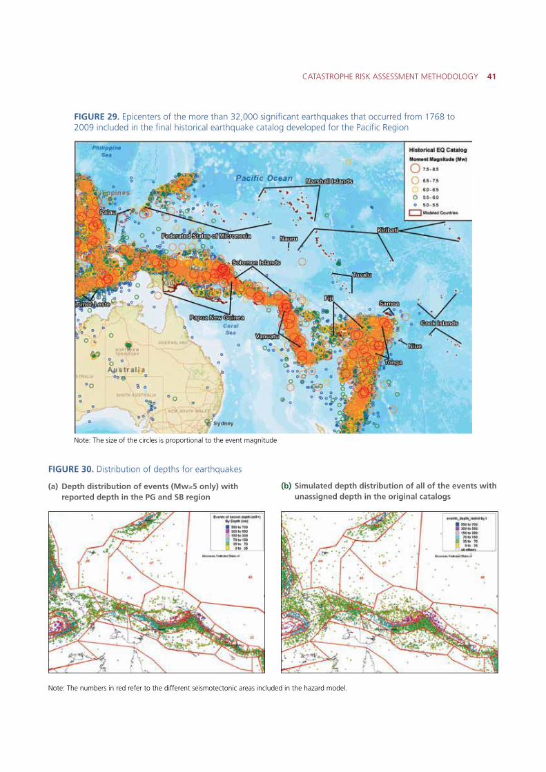
CATASTROPHE RISK ASSESSMENT METHODOLOGY 41
FIGURE 30. Distribution of depths for earthquakes
(a) Depth distribution of events (Mw�5 only) with reported depth in the PG and SB region
(b) Simulated depth distribution of all of the events with unassigned depth in the original catalogs
FIGURE 29. Epicenters of the more than 32,000 significant earthquakes that occurred from 1768 to 2009 included in the final historical earthquake catalog developed for the Pacific Region
Note: The size of the circles is proportional to the event magnitude
Note: The numbers in red refer to the different seismotectonic areas included in the hazard model.
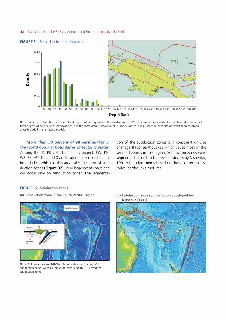
42 Pacific Catastrophe Risk Assessment and Financing Initiative (PCRAFI)
FIGURE 31. Focal depths of earthquakes
Note: Empirical distribution of known focal depths of earthquakes in the shaded area of PG is shown in green while the simulated distribution of focal depths of events with unknown depth in the same area is shown in blue. The numbers in red (insert) refer to the different seismotectonic areas included in the hazard model.
0 80 160 24040 120 200 28020 100 180 26060 140 22010 90 170 25050 130 21030 110 190 27070 150 230
Depth (km)
Den
sity
0.25
0.2
0.15
0.1
0.05
0
More than 90 percent of all earthquakes in the world occur at boundaries of tectonic plates. Among the 15 PICs studied in this project, PW, PG, WS, SB, VU, TL, and TO are located on or close to plate boundaries, which in this area take the form of sub-duction zones (Figure 32). Very large events have and will occur only on subduction zones. The segmenta-
tion of the subduction zones is a constraint on size of mega-thrust earthquakes which cause most of the seismic hazards in this region. Subduction zones were segmented according to previous studies by Nishenko, 1991 with adjustments based on the most recent his-torical earthquake ruptures.
FIGURE 32. Subduction zones
(a) Subduction zone in the South Pacific Region (b) Subduction zone segmentation developed by Nishenko (1991)
Note: Abbreviations are: NB-New Britain subduction zone; S-SB subduction zone; VA-VU subduction zone; and TK-TO-Kermadec subduction zone.
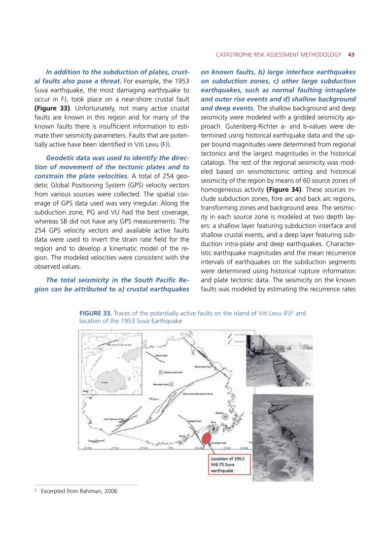
CATASTROPHE RISK ASSESSMENT METHODOLOGY 43
In addition to the subduction of plates, crust-al faults also pose a threat. For example, the 1953 Suva earthquake, the most damaging earthquake to occur in FJ, took place on a near-shore crustal fault (Figure 33). Unfortunately, not many active crustal faults are known in this region and for many of the known faults there is insufficient information to esti-mate their seismicity parameters. Faults that are poten-tially active have been identified in Viti Levu (FJ).
Geodetic data was used to identify the direc-tion of movement of the tectonic plates and to constrain the plate velocities. A total of 254 geo-detic Global Positioning System (GPS) velocity vectors from various sources were collected. The spatial cov-erage of GPS data used was very irregular. Along the subduction zone, PG and VU had the best coverage, whereas SB did not have any GPS measurements. The 254 GPS velocity vectors and available active faults data were used to invert the strain rate field for the region and to develop a kinematic model of the re-gion. The modeled velocities were consistent with the observed values.
The total seismicity in the South Pacific Re-gion can be attributed to a) crustal earthquakes
on known faults, b) large interface earthquakes on subduction zones, c) other large subduction earthquakes, such as normal faulting intraplate and outer rise events and d) shallow background and deep events. The shallow background and deep seismicity were modeled with a gridded seismicity ap-proach. Gutenberg-Richter a- and b-values were de-termined using historical earthquake data and the up-per bound magnitudes were determined from regional tectonics and the largest magnitudes in the historical catalogs. The rest of the regional seismicity was mod-eled based on seismotectonic setting and historical seismicity of the region by means of 60 source zones of homogeneous activity (Figure 34). These sources in-clude subduction zones, fore arc and back arc regions, transforming zones and background area. The seismic-ity in each source zone is modeled at two depth lay-ers: a shallow layer featuring subduction interface and shallow crustal events, and a deep layer featuring sub-duction intra-plate and deep earthquakes. Character-istic earthquake magnitudes and the mean recurrence intervals of earthquakes on the subduction segments were determined using historical rupture information and plate tectonic data. The seismicity on the known faults was modeled by estimating the recurrence rates
2 Excerpted from Rahiman, 2006.
FIGURE 33. Traces of the potentially active faults on the island of Viti Levu (FJ)2 and location of the 1953 Suva Earthquake
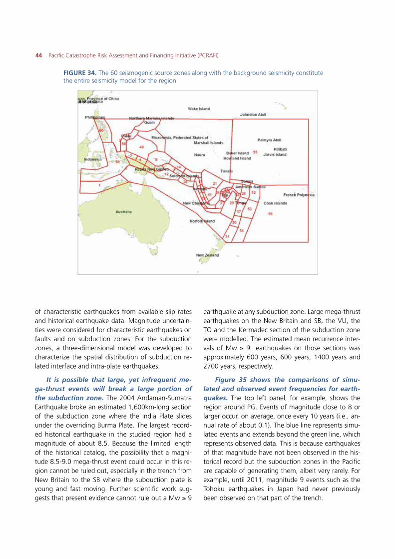
44 Pacific Catastrophe Risk Assessment and Financing Initiative (PCRAFI)
of characteristic earthquakes from available slip rates and historical earthquake data. Magnitude uncertain-ties were considered for characteristic earthquakes on faults and on subduction zones. For the subduction zones, a three-dimensional model was developed to characterize the spatial distribution of subduction re-lated interface and intra-plate earthquakes.
It is possible that large, yet infrequent me-ga-thrust events will break a large portion of the subduction zone. The 2004 Andaman-Sumatra Earthquake broke an estimated 1,600km-long section of the subduction zone where the India Plate slides under the overriding Burma Plate. The largest record-ed historical earthquake in the studied region had a magnitude of about 8.5. Because the limited length of the historical catalog, the possibility that a magni-tude 8.5-9.0 mega-thrust event could occur in this re-gion cannot be ruled out, especially in the trench from New Britain to the SB where the subduction plate is young and fast moving. Further scientific work sug-gests that present evidence cannot rule out a Mw � 9
earthquake at any subduction zone. Large mega-thrust earthquakes on the New Britain and SB, the VU, the TO and the Kermadec section of the subduction zone were modelled. The estimated mean recurrence inter-vals of Mw � 9 earthquakes on those sections was approximately 600 years, 600 years, 1400 years and 2700 years, respectively.
Figure 35 shows the comparisons of simu-lated and observed event frequencies for earth-quakes. The top left panel, for example, shows the region around PG. Events of magnitude close to 8 or larger occur, on average, once every 10 years (i.e., an-nual rate of about 0.1). The blue line represents simu-lated events and extends beyond the green line, which represents observed data. This is because earthquakes of that magnitude have not been observed in the his-torical record but the subduction zones in the Pacific are capable of generating them, albeit very rarely. For example, until 2011, magnitude 9 events such as the Tohoku earthquakes in Japan had never previously been observed on that part of the trench.
FIGURE 34. The 60 seismogenic source zones along with the background seismicity constitute the entire seismicity model for the region
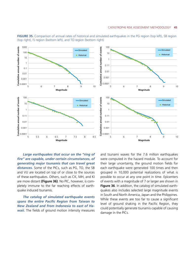
CATASTROPHE RISK ASSESSMENT METHODOLOGY 45
FIGURE 35. Comparison of annual rates of historical and simulated earthquakes in the PG region (top left), SB region (top right), FJ region (bottom left), and TO region (bottom right)
Simulated
Historical
Simulated
Historical
Simulated
Historical
Cu
mu
lati
ve a
nn
ual
nu
mb
er o
f ev
ents
Cu
mu
lati
ve a
nn
ual
nu
mb
er o
f ev
ents
Cu
mu
lati
ve a
nn
ual
nu
mb
er o
f ev
ents
Cu
mu
lati
ve a
nn
ual
nu
mb
er o
f ev
ents
Magnitude
Magnitude
Magnitude
Magnitude
1000
100
10
1
0.1
0.01
0.001
0.0001
100
10
1
0.11
0.01
0.001
0.0001
100
10
1
0.11
0.01
0.001
0.0001
100
10
1
0.11
0.01
0.001
0.0001
5
5
5
5
7
6
7
7
10
8.58
10
10
6
5.5
6
6
9
7.5
9
9
8
6.5 7
8
8
Simulated
Historical
Large earthquakes that occur on the “ring of fire” are capable, under certain circumstances, of generating major tsunamis that can travel great distances. Some of the PICs, such as PG, TO, the SB and VU are located on top of or close to the sources of these earthquakes. Others, such as CK, MH, and KI are more distant (Figure 36). No PIC, however, is com-pletely immune to the far reaching effects of earth-quake induced tsunamis.
The catalog of simulated earthquake events spans the entire Pacific Region from Taiwan to New Zealand and from Indonesia to east of Ha-waii. The fields of ground motion intensity measures
and tsunami waves for the 7.6 million earthquakes were computed in the hazard module. To account for their large uncertainty, the ground motion fields for each earthquake were generated 100 times and then grouped in 10,000 potential realizations of what is possible to occur at any one point in time. Epicenters of events with a magnitude of 7 or larger are shown in Figure 36. In addition, the catalog of simulated earth-quakes also includes selected large magnitude events in South and North America, Japan and the Philippines. While these events are too far to cause a significant level of ground shaking in the Pacific Region, they could potentially generate tsunamis capable of causing damage in the PICs.
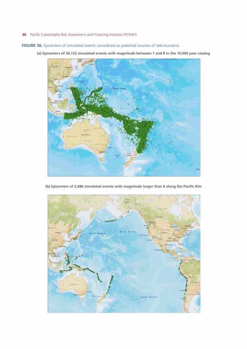
46 Pacific Catastrophe Risk Assessment and Financing Initiative (PCRAFI)
FIGURE 36. Epicenters of simulated events considered as potential sources of tele-tsunamis
(a) Epicenters of 50,722 simulated events with magnitude between 7 and 8 in the 10,000 year catalog
(b) Epicenters of 2,686 simulated events with magnitude larger than 8 along the Pacific Rim
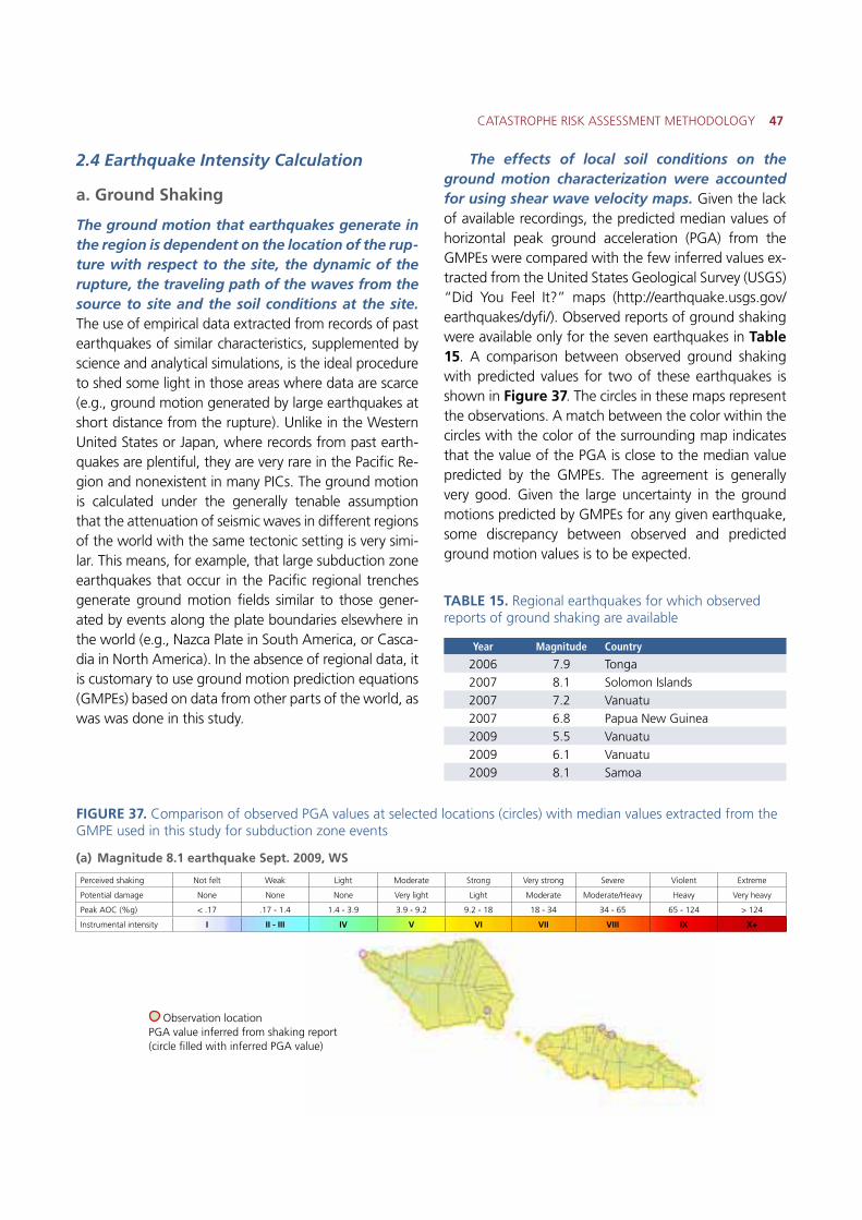
CATASTROPHE RISK ASSESSMENT METHODOLOGY 47
2.4 Earthquake Intensity Calculation
a. Ground Shaking
The ground motion that earthquakes generate in the region is dependent on the location of the rup-ture with respect to the site, the dynamic of the rupture, the traveling path of the waves from the source to site and the soil conditions at the site. The use of empirical data extracted from records of past earthquakes of similar characteristics, supplemented by science and analytical simulations, is the ideal procedure to shed some light in those areas where data are scarce (e.g., ground motion generated by large earthquakes at short distance from the rupture). Unlike in the Western United States or Japan, where records from past earth-quakes are plentiful, they are very rare in the Pacific Re-gion and nonexistent in many PICs. The ground motion is calculated under the generally tenable assumption that the attenuation of seismic waves in different regions of the world with the same tectonic setting is very simi-lar. This means, for example, that large subduction zone earthquakes that occur in the Pacific regional trenches generate ground motion fields similar to those gener-ated by events along the plate boundaries elsewhere in the world (e.g., Nazca Plate in South America, or Casca-dia in North America). In the absence of regional data, it is customary to use ground motion prediction equations (GMPEs) based on data from other parts of the world, as was was done in this study.
The effects of local soil conditions on the ground motion characterization were accounted for using shear wave velocity maps. Given the lack of available recordings, the predicted median values of horizontal peak ground acceleration (PGA) from the GMPEs were compared with the few inferred values ex-tracted from the United States Geological Survey (USGS) “Did You Feel It?” maps (http://earthquake.usgs.gov/earthquakes/dyfi/). Observed reports of ground shaking were available only for the seven earthquakes in Table 15. A comparison between observed ground shaking with predicted values for two of these earthquakes is shown in Figure 37. The circles in these maps represent the observations. A match between the color within the circles with the color of the surrounding map indicates that the value of the PGA is close to the median value predicted by the GMPEs. The agreement is generally very good. Given the large uncertainty in the ground motions predicted by GMPEs for any given earthquake, some discrepancy between observed and predicted ground motion values is to be expected.
TABLE 15. Regional earthquakes for which observed reports of ground shaking are available
Year Magnitude Country
2006 7.9 Tonga2007 8.1 Solomon Islands2007 7.2 Vanuatu2007 6.8 Papua New Guinea2009 5.5 Vanuatu2009 6.1 Vanuatu2009 8.1 Samoa
Observation locationPGA value inferred from shaking report (circle filled with inferred PGA value)
Perceived shaking Not felt Weak Light Moderate Strong Very strong Severe Violent Extreme
Potential damage None None None Very light Light Moderate Moderate/Heavy Heavy Very heavy
Peak AOC (%g) < .17 .17 - 1.4 1.4 - 3.9 3.9 - 9.2 9.2 - 18 18 - 34 34 - 65 65 - 124 > 124
Instrumental intensity I II - III IV V VI VII VIII IX X+
FIGURE 37. Comparison of observed PGA values at selected locations (circles) with median values extracted from the GMPE used in this study for subduction zone events
(a) Magnitude 8.1 earthquake Sept. 2009, WS
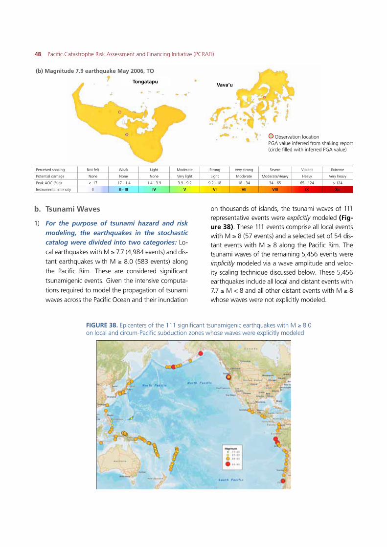
48 Pacific Catastrophe Risk Assessment and Financing Initiative (PCRAFI)
(b) Magnitude 7.9 earthquake May 2006, TO
Perceived shaking Not felt Weak Light Moderate Strong Very strong Severe Violent Extreme
Potential damage None None None Very light Light Moderate Moderate/Heavy Heavy Very heavy
Peak AOC (%g) < .17 .17 - 1.4 1.4 - 3.9 3.9 - 9.2 9.2 - 18 18 - 34 34 - 65 65 - 124 > 124
Instrumental intensity I II - III IV V VI VII VIII IX X+
b. Tsunami Waves
1) For the purpose of tsunami hazard and risk modeling, the earthquakes in the stochastic catalog were divided into two categories: Lo-cal earthquakes with M � 7.7 (4,984 events) and dis-tant earthquakes with M � 8.0 (583 events) along the Pacific Rim. These are considered significant tsunamigenic events. Given the intensive computa-tions required to model the propagation of tsunami waves across the Pacific Ocean and their inundation
on thousands of islands, the tsunami waves of 111 representative events were explicitly modeled (Fig-ure 38). These 111 events comprise all local events with M � 8 (57 events) and a selected set of 54 dis-tant events with M � 8 along the Pacific Rim. The tsunami waves of the remaining 5,456 events were implicitly modeled via a wave amplitude and veloc-ity scaling technique discussed below. These 5,456 earthquakes include all local and distant events with 7.7 � M < 8 and all other distant events with M � 8 whose waves were not explicitly modeled.
Observation locationPGA value inferred from shaking report (circle filled with inferred PGA value)
TongatapuVava’u
FIGURE 38. Epicenters of the 111 significant tsunamigenic earthquakes with M � 8.0 on local and circum-Pacific subduction zones whose waves were explicitly modeled
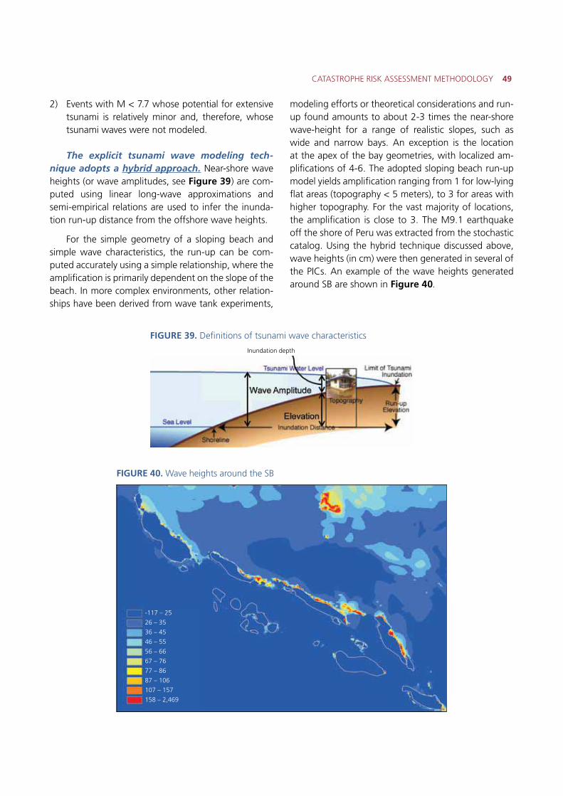
CATASTROPHE RISK ASSESSMENT METHODOLOGY 49
2) Events with M < 7.7 whose potential for extensive tsunami is relatively minor and, therefore, whose tsunami waves were not modeled.
The explicit tsunami wave modeling tech-nique adopts a hybrid approach. Near-shore wave heights (or wave amplitudes, see Figure 39) are com-puted using linear long-wave approximations and semi-empirical relations are used to infer the inunda-tion run-up distance from the offshore wave heights.
For the simple geometry of a sloping beach and simple wave characteristics, the run-up can be com-puted accurately using a simple relationship, where the amplification is primarily dependent on the slope of the beach. In more complex environments, other relation-ships have been derived from wave tank experiments,
modeling efforts or theoretical considerations and run-up found amounts to about 2-3 times the near-shore wave-height for a range of realistic slopes, such as wide and narrow bays. An exception is the location at the apex of the bay geometries, with localized am-plifications of 4-6. The adopted sloping beach run-up model yields amplification ranging from 1 for low-lying flat areas (topography < 5 meters), to 3 for areas with higher topography. For the vast majority of locations, the amplification is close to 3. The M9.1 earthquake off the shore of Peru was extracted from the stochastic catalog. Using the hybrid technique discussed above, wave heights (in cm) were then generated in several of the PICs. An example of the wave heights generated around SB are shown in Figure 40.
FIGURE 40. Wave heights around the SB
Inundation depth
FIGURE 39. Definitions of tsunami wave characteristics
-117 – 25
26 – 35
36 – 45
46 – 55
56 – 66
67 – 76
77 – 86
87 – 106
107 – 157
158 – 2,469
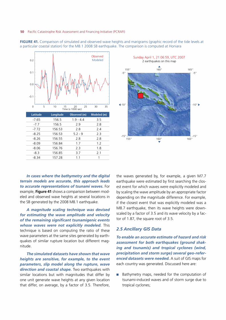
50 Pacific Catastrophe Risk Assessment and Financing Initiative (PCRAFI)
In cases where the bathymetry and the digital terrain models are accurate, this approach leads to accurate representations of tsunami waves. For example, Figure 41 shows a comparison between mod-eled and observed wave heights at several locations in the SB generated by the 2008 M8.1 earthquake.
A magnitude scaling technique was devised for estimating the wave amplitude and velocity of the remaining significant tsunamigenic events whose waves were not explicitly modeled. This technique is based on computing the ratio of these wave parameters at the same sites generated by earth-quakes of similar rupture location but different mag-nitude.
The simulated datasets have shown that wave heights are sensitive, for example, to the event parameters, slip model along the rupture, wave direction and coastal shape. Two earthquakes with similar locations but with magnitudes that differ by one unit generate wave heights at any given location that differ, on average, by a factor of 3.5. Therefore,
the waves generated by, for example, a given M7.7 earthquake were estimated by first searching the clos-est event for which waves were explicitly modeled and by scaling the wave amplitude by an appropriate factor depending on the magnitude difference. For example, if the closest event that was explicitly modeled was a M8.7 earthquake, then its wave heights were down-scaled by a factor of 3.5 and its wave velocity by a fac-tor of 1.87, the square root of 3.5.
2.5 Ancillary GIS Data
To enable an accurate estimate of hazard and risk assessment for both earthquakes (ground shak-ing and tsunamis) and tropical cyclones (wind, precipitation and storm surge) several geo-refer-enced datasets were needed. A suit of GIS maps for each country was generated. Discussed here are:
�� Bathymetry maps, needed for the computation of tsunami-induced waves and of storm surge due to tropical cyclones;
FIGURE 41. Comparison of simulated and observed wave heights and marigrams (graphic record of the tide levels at a particular coastal station) for the M8.1 2008 SB earthquake. The comparison is computed at Honiara
Latitude Longitude Observed (m) Modeled (m)
-7.65 156.5 1.9 - 4.4 3.5-7.7 156.5 2.9 2.8
-7.72 156.53 2.8 2.4-8.25 156.53 5.2 - 9 2.3-8.26 156.55 2.8 2.8-8.09 156.84 1.7 1.2-8.06 156.76 2.3 1.8-8.3 156.85 3.7 2.1
-8.34 157.28 1.1 1
0.2
0.1
0.0
-0.1
0 5 10 15 20 25 30 35-10” -10”
-15”165”
165”
160”
160”
155”
155”-5”
-15”
-5”
ObservedModeled
Time (x 1000 sec)
Sunday April 1, 21:06:59, UTC 20072 earthquakes on this map
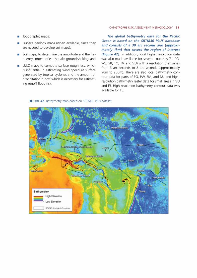
CATASTROPHE RISK ASSESSMENT METHODOLOGY 51
�� Topographic maps;
�� Surface geology maps (when available, since they are needed to develop soil maps);
�� Soil maps, to determine the amplitude and the fre-quency content of earthquake ground shaking; and
�� LULC maps to compute surface roughness, which is influential in estimating wind speed at surface generated by tropical cyclones and the amount of precipitation runoff which is necessary for estimat-ing runoff flood risk.
The global bathymetry data for the Pacific Ocean is based on the SRTM30 PLUS database and consists of a 30 arc second grid (approxi-mately 1km) that covers the region of interest (Figure 42). In addition, local higher resolution data was also made available for several countries (FJ, PG, WS, SB, TO, TV, and VU) with a resolution that varies from 3 arc seconds to 8 arc seconds (approximately 90m to 250m). There are also local bathymetry con-tour data for parts of PG, PW, FM, and NU and high-resolution bathymetry raster data for small areas in VU and FJ. High-resolution bathymetry contour data was available for TL.
FIGURE 42. Bathymetry map based on SRTM30 Plus dataset
52 Pacific Catastrophe Risk Assessment and Financing Initiative (PCRAFI)
Topography data was provided by NASA’s Shuttle Radar Topography Mission. This dataset covers the entire domain of the 15 covered nations and had a resolution of 3 arc seconds (roughly 90 meters). Geologic maps show the distribution of geologic fea-tures, including different types of rocks of a given age range. They are useful to infer the depth, and stiffness of soil sediments that may be present and to estimate the amount of amplifications that seismic waves may be subject to when filtered by these soil units. The geologic maps that were collected during the course of the project are limited in number, coverage, and in some cases quality, which was expected. No country or regional scale site-condition maps based on detailed surface geology maps are available for the 15 PICs. In this case, it is customary to use the method developed by Allen and Wald, which uses topographic data as a proxy for site conditions. The methodology circumvents data inconsistencies and is widely used for hazard and risk assessment purposes around the globe. The soil maps derived using this methodology show the shear wave velocity of seismic waves in the top 30m of soil, which is denoted as Vs30. High values of Vs30 (e.g., greater than 760m/s) refer to soft and hard rock site conditions, which show no significant amplification of incipient seismic waves. Very low values of Vs30 (e.g., lower than 180m/s) refer to very soft soil sites where significant amplification is expected. Average medium to stiff soil conditions have Vs30 values in the 300 to 500m/s range. Although these maps are developed according to the current state-of-the-art approach, it
should be noted that in some cases discrepancies may be found between the values of Vs30 estimated by this method and those that may be measured in the field. If detailed surface geology maps at a regional scale such as those customarily developed for micro-zonation studies were to become available, they should be used for earthquake ground motion assessment in lieu of those developed here.
LULC maps are used to determine roughness factors and precipitation runoff percentages. Land cover refers to the physical and biological cover over the land surface, including water, vegetation, bare soil and artificial structures. Land use usually refers to signs of human activities such as agriculture, forestry and building construction that altered the original land surface processes. The LULC maps were developed us-ing remotely sensed data (i.e., satellite imagery) of dif-ferent resolution and vintage, validated with the aid of some ground truthing, virtual truthing (using high-resolution imagery of more recent vintage and other internet resources), agriculture census and other ancil-lary data collected during the course of the project. Given the methodology adopted, it is to be expected that in some instances the information included in the LULC maps may be obsolete and inaccurate. The LULC maps developed here are, however, perfectly suitable for the scope of assessing wind and flood hazard and were also developed for establishing a crop exposure database (see Section 1.4).
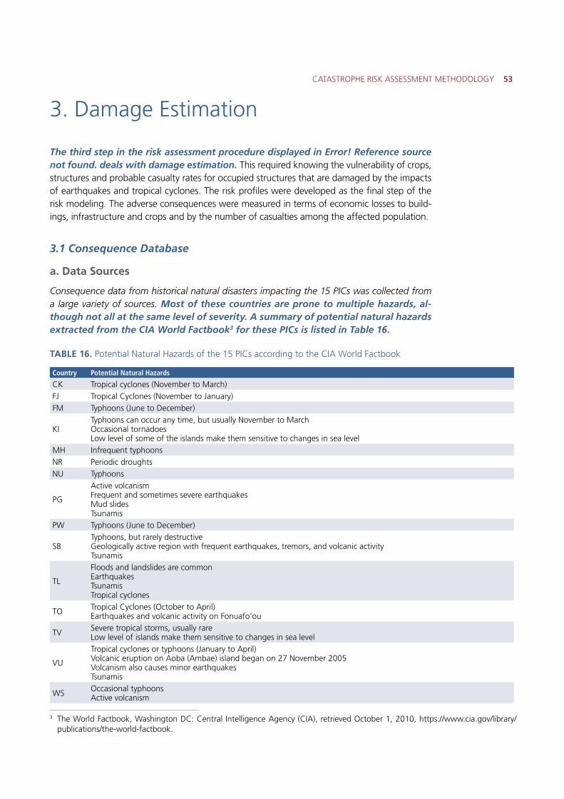
CATASTROPHE RISK ASSESSMENT METHODOLOGY 53
3. Damage Estimation
The third step in the risk assessment procedure displayed in Error! Reference source not found. deals with damage estimation. This required knowing the vulnerability of crops, structures and probable casualty rates for occupied structures that are damaged by the impacts of earthquakes and tropical cyclones. The risk profiles were developed as the final step of the risk modeling. The adverse consequences were measured in terms of economic losses to build-ings, infrastructure and crops and by the number of casualties among the affected population.
3.1 Consequence Database
a. Data Sources
Consequence data from historical natural disasters impacting the 15 PICs was collected from a large variety of sources. Most of these countries are prone to multiple hazards, al-though not all at the same level of severity. A summary of potential natural hazards extracted from the CIA World Factbook3 for these PICs is listed in Table 16.
TABLE 16. Potential Natural Hazards of the 15 PICs according to the CIA World Factbook
Country Potential Natural Hazards
CK Tropical cyclones (November to March)FJ Tropical Cyclones (November to January)FM Typhoons (June to December)
KITyphoons can occur any time, but usually November to MarchOccasional tornadoesLow level of some of the islands make them sensitive to changes in sea level
MH Infrequent typhoonsNR Periodic droughtsNU Typhoons
PG
Active volcanismFrequent and sometimes severe earthquakesMud slidesTsunamis
PW Typhoons (June to December)
SBTyphoons, but rarely destructiveGeologically active region with frequent earthquakes, tremors, and volcanic activity Tsunamis
TL
Floods and landslides are commonEarthquakesTsunamisTropical cyclones
TO Tropical Cyclones (October to April)Earthquakes and volcanic activity on Fonuafo’ou
TV Severe tropical storms, usually rareLow level of islands make them sensitive to changes in sea level
VU
Tropical cyclones or typhoons (January to April)Volcanic eruption on Aoba (Ambae) island began on 27 November 2005Volcanism also causes minor earthquakesTsunamis
WS Occasional typhoonsActive volcanism
3 The World Factbook, Washington DC: Central Intelligence Agency (CIA), retrieved October 1, 2010, https://www.cia.gov/library/publications/the-world-factbook.
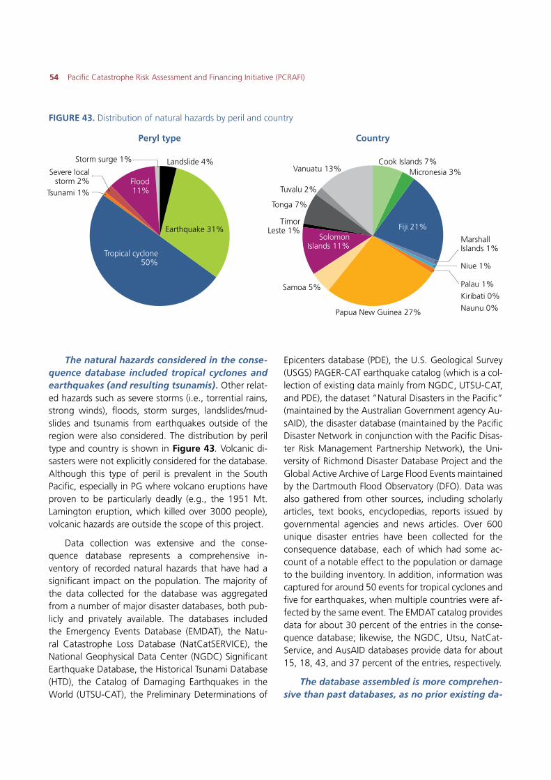
54 Pacific Catastrophe Risk Assessment and Financing Initiative (PCRAFI)
The natural hazards considered in the conse-quence database included tropical cyclones and earthquakes (and resulting tsunamis). Other relat-ed hazards such as severe storms (i.e., torrential rains, strong winds), floods, storm surges, landslides/mud-slides and tsunamis from earthquakes outside of the region were also considered. The distribution by peril type and country is shown in Figure 43. Volcanic di-sasters were not explicitly considered for the database. Although this type of peril is prevalent in the South Pacific, especially in PG where volcano eruptions have proven to be particularly deadly (e.g., the 1951 Mt. Lamington eruption, which killed over 3000 people), volcanic hazards are outside the scope of this project.
Data collection was extensive and the conse-quence database represents a comprehensive in-ventory of recorded natural hazards that have had a significant impact on the population. The majority of the data collected for the database was aggregated from a number of major disaster databases, both pub-licly and privately available. The databases included the Emergency Events Database (EMDAT), the Natu-ral Catastrophe Loss Database (NatCatSERVICE), the National Geophysical Data Center (NGDC) Significant Earthquake Database, the Historical Tsunami Database (HTD), the Catalog of Damaging Earthquakes in the World (UTSU-CAT), the Preliminary Determinations of
Epicenters database (PDE), the U.S. Geological Survey (USGS) PAGER-CAT earthquake catalog (which is a col-lection of existing data mainly from NGDC, UTSU-CAT, and PDE), the dataset “Natural Disasters in the Pacific” (maintained by the Australian Government agency Au-sAID), the disaster database (maintained by the Pacific Disaster Network in conjunction with the Pacific Disas-ter Risk Management Partnership Network), the Uni-versity of Richmond Disaster Database Project and the Global Active Archive of Large Flood Events maintained by the Dartmouth Flood Observatory (DFO). Data was also gathered from other sources, including scholarly articles, text books, encyclopedias, reports issued by governmental agencies and news articles. Over 600 unique disaster entries have been collected for the consequence database, each of which had some ac-count of a notable effect to the population or damage to the building inventory. In addition, information was captured for around 50 events for tropical cyclones and five for earthquakes, when multiple countries were af-fected by the same event. The EMDAT catalog provides data for about 30 percent of the entries in the conse-quence database; likewise, the NGDC, Utsu, NatCat-Service, and AusAID databases provide data for about 15, 18, 43, and 37 percent of the entries, respectively.
The database assembled is more comprehen-sive than past databases, as no prior existing da-
FIGURE 43. Distribution of natural hazards by peril and country
Cook Islands 7%Micronesia 3%
Papua New Guinea 27%
Samoa 5%
Solomon Islands 11%
Tonga 7%
Tuvalu 2%
Vanuatu 13%Landslide 4%Storm surge 1%
Flood11%
Tropical cyclone 50%
Severe local storm 2%
Tsunami 1%
Earthquake 31% Fiji 21%
Kiribati 0%
Naunu 0%
Marshall Islands 1%
Niue 1%
Palau 1%
TimorLeste 1%
Peryl type Country
CATASTROPHE RISK ASSESSMENT METHODOLOGY 55
tabase covers a majority of the entries. However, many entries, especially those from very damaging events, contain data from multiple sources, leading to discrepancies in the quantitative data, particularly eco-nomic losses. By design, the discrepancies have been preserved and each piece of data in the consequence database is appropriately referenced.
Great effort was taken to map the events in the consequence database to the historical cata-log of tropical cyclones and earthquakes devel-oped in this study and described earlier. Over 80 percent of the earthquake entries have been mapped to events in the earthquake historical catalog. Likewise, over 85 percent of the tropical cyclone entries have been mapped to events in the tropical cyclone histori-cal catalog. Most of the events that are not tracked are older events (i.e., prior to 1900 for earthquakes and prior to 1948 for cyclones), which are, for the most part, are not archived in the historical catalog.
b. Explanation of Data Fields
The referenced sources discussed above typi-cally report a brief summary of the disaster con-sequence (e.g., number of people affected and/or number of lives lost), and some accounts are strictly qualitative (e.g., “buildings and crops were damaged”). For each entry in the consequence database, data from each field is typically an aggre-gate account of the total consequence from a particu-lar disaster event (including related secondary events/effects), with most or all of the damage occurring in the country listed. For earthquake events, the losses are aggregated for ground shaking and the resulting wave impact(s) and specific details on the relative losses are noted for some events. Some events, like those listed as floods, landslides, severe storms and storm surges, were not directly linked to reported earthquakes or tropical cyclones. In addition, some tsunami events were a result of earthquakes occurring outside the South Pacific Region (e.g., the 1877 tsunami in FJ was caused by very large earthquake near Chile).
The main data fields of the consequence database are:
�� Total Number of People Affected – A measure of the estimated number of people affected by the
event, including those that became homeless, in-jured, displaced, evacuated, or disrupted (e.g., af-fected by loss of utilities) by the peril.
�� Number of People Homeless – A subset of the number of people affected, indicating the number of people required to vacate their residence due to the peril, such as those evacuated or displaced.
�� Estimated Total Economic Loss – The estimated to-tal economic impact of the event, usually consist-ing of direct (e.g., damage to infrastructure, crops, housing) and indirect (e.g., loss of revenues, un-employment, market destabilization) consequences on the local economy. Estimated loss is typically re-ported in U.S. dollars (US$), corresponding to the monetary loss at the time of the event (e.g., cur-rent/nominal US$). Some data were reported in lo-cal currencies and were converted appropriately by using filtered rates for specific (time-of-event) dates based on information supplied by leading market data. Losses are reported as the monetary cost at the time of the event, as well as costs trended to current values using a macro-economic exposure growth parameter (as discussed below). Losses are typically listed in the consequence database as the total direct economic loss. Break-down losses are available for those events where detailed assess-ment reports were issued, e.g., losses per sector (social sector, private sector, infrastructure, etc.), crop losses, and locations for deaths and building damages.
�� Total Life Loss – The total number of people re-ported dead, missing or presumed dead as a result of the event, including any resulting deaths from starvation, injury, or disease.
�� Total Injured – The total number of people suffering from physical injuries, trauma or an illness requiring medical treatment as a result the event.
�� Buildings Damaged or Destroyed – The total num-ber of buildings (typically listed as “houses”) re-ported to be damaged or destroyed as a result the event. While quantitative data of damage is some-times reported (e.g., the total number of houses destroyed), much of the data is qualitative (e.g., “some houses were damaged.”)
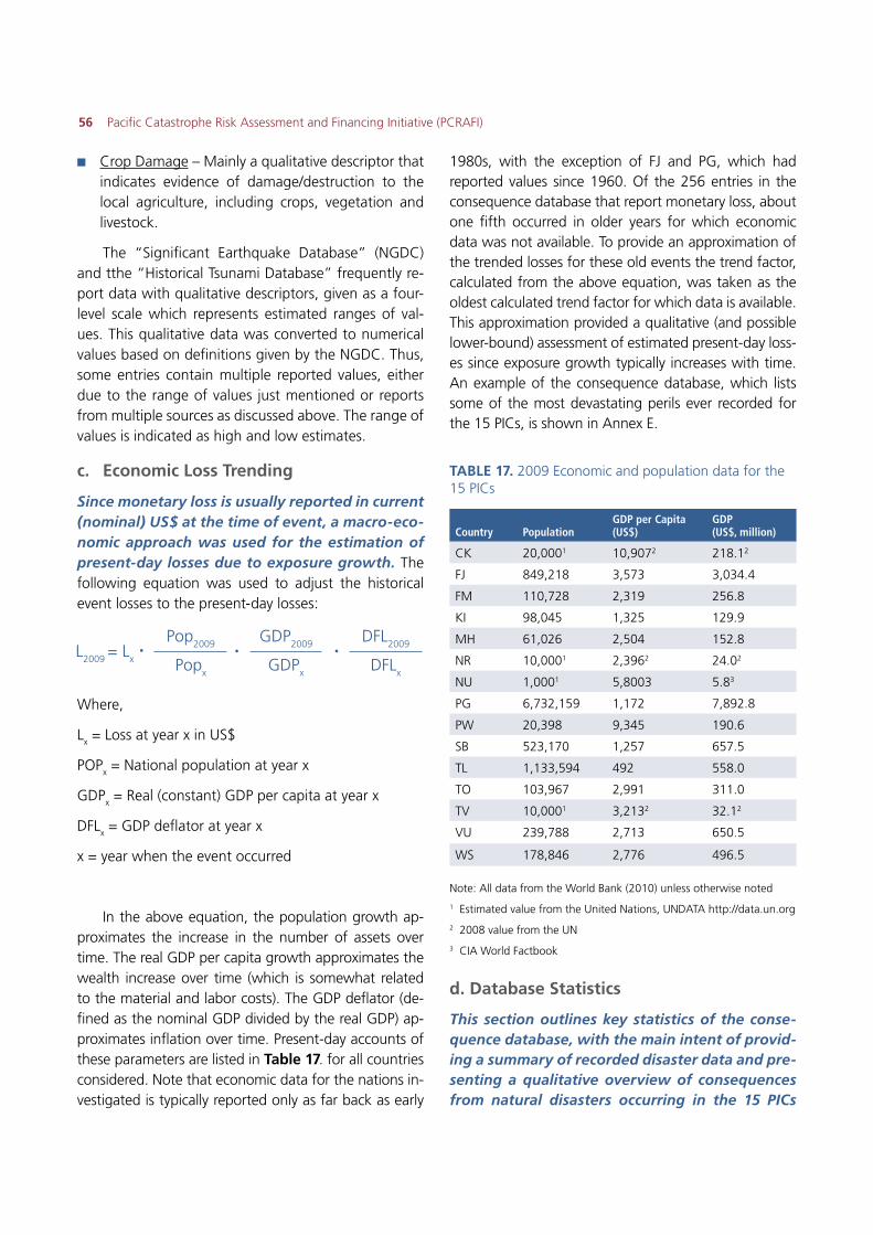
56 Pacific Catastrophe Risk Assessment and Financing Initiative (PCRAFI)
�� Crop Damage – Mainly a qualitative descriptor that indicates evidence of damage/destruction to the local agriculture, including crops, vegetation and livestock.
The “Significant Earthquake Database” (NGDC) and tthe “Historical Tsunami Database” frequently re-port data with qualitative descriptors, given as a four-level scale which represents estimated ranges of val-ues. This qualitative data was converted to numerical values based on definitions given by the NGDC. Thus, some entries contain multiple reported values, either due to the range of values just mentioned or reports from multiple sources as discussed above. The range of values is indicated as high and low estimates.
c. Economic Loss Trending
Since monetary loss is usually reported in current (nominal) US$ at the time of event, a macro-eco-nomic approach was used for the estimation of present-day losses due to exposure growth. The following equation was used to adjust the historical event losses to the present-day losses:
Where,
Lx = Loss at year x in US$
POPx = National population at year x
GDPx = Real (constant) GDP per capita at year x
DFLx = GDP deflator at year x
x = year when the event occurred
In the above equation, the population growth ap-proximates the increase in the number of assets over time. The real GDP per capita growth approximates the wealth increase over time (which is somewhat related to the material and labor costs). The GDP deflator (de-fined as the nominal GDP divided by the real GDP) ap-proximates inflation over time. Present-day accounts of these parameters are listed in Table 17. for all countries considered. Note that economic data for the nations in-vestigated is typically reported only as far back as early
1980s, with the exception of FJ and PG, which had reported values since 1960. Of the 256 entries in the consequence database that report monetary loss, about one fifth occurred in older years for which economic data was not available. To provide an approximation of the trended losses for these old events the trend factor, calculated from the above equation, was taken as the oldest calculated trend factor for which data is available. This approximation provided a qualitative (and possible lower-bound) assessment of estimated present-day loss-es since exposure growth typically increases with time. An example of the consequence database, which lists some of the most devastating perils ever recorded for the 15 PICs, is shown in Annex E.
TABLE 17. 2009 Economic and population data for the 15 PICs
Country PopulationGDP per Capita (US$)
GDP(US$, million)
CK 20,0001 10,9072 218.12
FJ 849,218 3,573 3,034.4
FM 110,728 2,319 256.8
KI 98,045 1,325 129.9
MH 61,026 2,504 152.8
NR 10,0001 2,3962 24.02
NU 1,0001 5,8003 5.83
PG 6,732,159 1,172 7,892.8
PW 20,398 9,345 190.6
SB 523,170 1,257 657.5
TL 1,133,594 492 558.0
TO 103,967 2,991 311.0
TV 10,0001 3,2132 32.12
VU 239,788 2,713 650.5
WS 178,846 2,776 496.5 Note: All data from the World Bank (2010) unless otherwise noted
1 Estimated value from the United Nations, UNDATA http://data.un.org
2 2008 value from the UN
3 CIA World Factbook
d. Database Statistics
This section outlines key statistics of the conse-quence database, with the main intent of provid-ing a summary of recorded disaster data and pre-senting a qualitative overview of consequences from natural disasters occurring in the 15 PICs
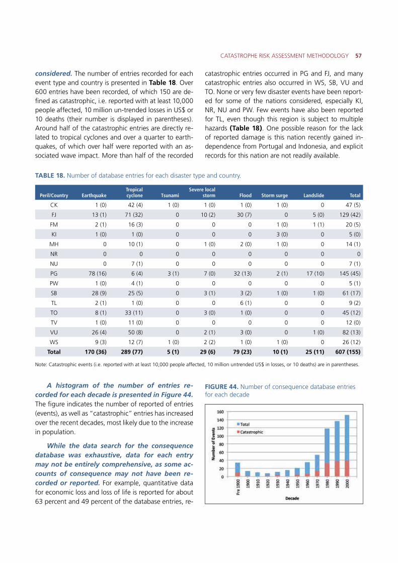
CATASTROPHE RISK ASSESSMENT METHODOLOGY 57
considered. The number of entries recorded for each event type and country is presented in Table 18. Over 600 entries have been recorded, of which 150 are de-fined as catastrophic, i.e. reported with at least 10,000 people affected, 10 million un-trended losses in US$ or 10 deaths (their number is displayed in parentheses). Around half of the catastrophic entries are directly re-lated to tropical cyclones and over a quarter to earth-quakes, of which over half were reported with an as-sociated wave impact. More than half of the recorded
catastrophic entries occurred in PG and FJ, and many catastrophic entries also occurred in WS, SB, VU and TO. None or very few disaster events have been report-ed for some of the nations considered, especially KI, NR, NU and PW. Few events have also been reported for TL, even though this region is subject to multiple hazards (Table 18). One possible reason for the lack of reported damage is this nation recently gained in-dependence from Portugal and Indonesia, and explicit records for this nation are not readily available.
TABLE 18. Number of database entries for each disaster type and country.
Peril/Country EarthquakeTropical cyclone Tsunami
Severe local storm Flood Storm surge Landslide Total
CK 1 (0) 42 (4) 1 (0) 1 (0) 1 (0) 1 (0) 0 47 (5)
FJ 13 (1) 71 (32) 0 10 (2) 30 (7) 0 5 (0) 129 (42)
FM 2 (1) 16 (3) 0 0 0 1 (0) 1 (1) 20 (5)
KI 1 (0) 1 (0) 0 0 0 3 (0) 0 5 (0)
MH 0 10 (1) 0 1 (0) 2 (0) 1 (0) 0 14 (1)
NR 0 0 0 0 0 0 0 0
NU 0 7 (1) 0 0 0 0 0 7 (1)
PG 78 (16) 6 (4) 3 (1) 7 (0) 32 (13) 2 (1) 17 (10) 145 (45)
PW 1 (0) 4 (1) 0 0 0 0 0 5 (1)
SB 28 (9) 25 (5) 0 3 (1) 3 (2) 1 (0) 1 (0) 61 (17)
TL 2 (1) 1 (0) 0 0 6 (1) 0 0 9 (2)
TO 8 (1) 33 (11) 0 3 (0) 1 (0) 0 0 45 (12)
TV 1 (0) 11 (0) 0 0 0 0 0 12 (0)
VU 26 (4) 50 (8) 0 2 (1) 3 (0) 0 1 (0) 82 (13)
WS 9 (3) 12 (7) 1 (0) 2 (2) 1 (0) 1 (0) 0 26 (12)
Total 170 (36) 289 (77) 5 (1) 29 (6) 79 (23) 10 (1) 25 (11) 607 (155)
Note: Catastrophic events (i.e. reported with at least 10,000 people affected, 10 million untrended US$ in losses, or 10 deaths) are in parentheses.
A histogram of the number of entries re-corded for each decade is presented in Figure 44. The figure indicates the number of reported of entries (events), as well as “catastrophic” entries has increased over the recent decades, most likely due to the increase in population.
While the data search for the consequence database was exhaustive, data for each entry may not be entirely comprehensive, as some ac-counts of consequence may not have been re-corded or reported. For example, quantitative data for economic loss and loss of life is reported for about 63 percent and 49 percent of the database entries, re-
FIGURE 44. Number of consequence database entries for each decade
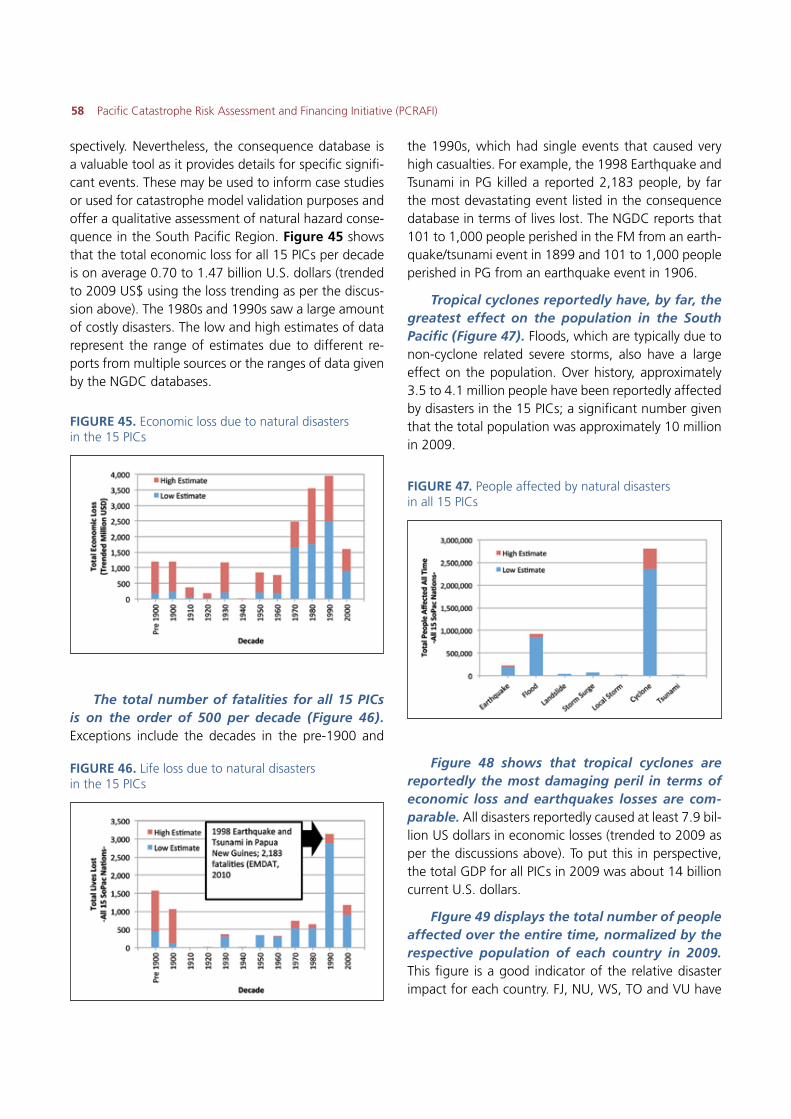
58 Pacific Catastrophe Risk Assessment and Financing Initiative (PCRAFI)
spectively. Nevertheless, the consequence database is a valuable tool as it provides details for specific signifi-cant events. These may be used to inform case studies or used for catastrophe model validation purposes and offer a qualitative assessment of natural hazard conse-quence in the South Pacific Region. Figure 45 shows that the total economic loss for all 15 PICs per decade is on average 0.70 to 1.47 billion U.S. dollars (trended to 2009 US$ using the loss trending as per the discus-sion above). The 1980s and 1990s saw a large amount of costly disasters. The low and high estimates of data represent the range of estimates due to different re-ports from multiple sources or the ranges of data given by the NGDC databases.
The total number of fatalities for all 15 PICs is on the order of 500 per decade (Figure 46). Exceptions include the decades in the pre-1900 and
the 1990s, which had single events that caused very high casualties. For example, the 1998 Earthquake and Tsunami in PG killed a reported 2,183 people, by far the most devastating event listed in the consequence database in terms of lives lost. The NGDC reports that 101 to 1,000 people perished in the FM from an earth-quake/tsunami event in 1899 and 101 to 1,000 people perished in PG from an earthquake event in 1906.
Tropical cyclones reportedly have, by far, the greatest effect on the population in the South Pacific (Figure 47). Floods, which are typically due to non-cyclone related severe storms, also have a large effect on the population. Over history, approximately 3.5 to 4.1 million people have been reportedly affected by disasters in the 15 PICs; a significant number given that the total population was approximately 10 million in 2009.
Figure 48 shows that tropical cyclones are reportedly the most damaging peril in terms of economic loss and earthquakes losses are com-parable. All disasters reportedly caused at least 7.9 bil-lion US dollars in economic losses (trended to 2009 as per the discussions above). To put this in perspective, the total GDP for all PICs in 2009 was about 14 billion current U.S. dollars.
FIgure 49 displays the total number of people affected over the entire time, normalized by the respective population of each country in 2009. This figure is a good indicator of the relative disaster impact for each country. FJ, NU, WS, TO and VU have
FIGURE 45. Economic loss due to natural disasters in the 15 PICs
FIGURE 47. People affected by natural disasters in all 15 PICs
FIGURE 46. Life loss due to natural disasters in the 15 PICs
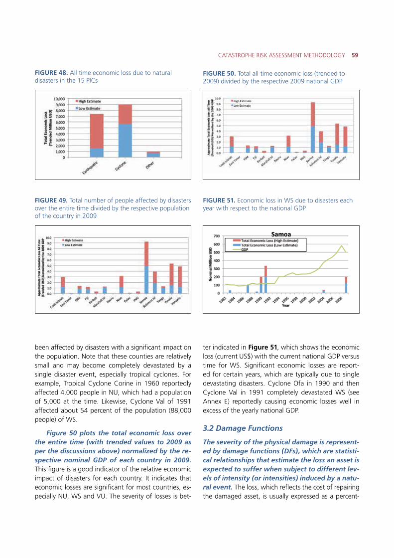
CATASTROPHE RISK ASSESSMENT METHODOLOGY 59
been affected by disasters with a significant impact on the population. Note that these counties are relatively small and may become completely devastated by a single disaster event, especially tropical cyclones. For example, Tropical Cyclone Corine in 1960 reportedly affected 4,000 people in NU, which had a population of 5,000 at the time. Likewise, Cyclone Val of 1991 affected about 54 percent of the population (88,000 people) of WS.
Figure 50 plots the total economic loss over the entire time (with trended values to 2009 as per the discussions above) normalized by the re-spective nominal GDP of each country in 2009. This figure is a good indicator of the relative economic impact of disasters for each country. It indicates that economic losses are significant for most countries, es-pecially NU, WS and VU. The severity of losses is bet-
ter indicated in Figure 51, which shows the economic loss (current US$) with the current national GDP versus time for WS. Significant economic losses are report-ed for certain years, which are typically due to single devastating disasters. Cyclone Ofa in 1990 and then Cyclone Val in 1991 completely devastated WS (see Annex E) reportedly causing economic losses well in excess of the yearly national GDP.
3.2 Damage Functions
The severity of the physical damage is represent-ed by damage functions (DFs), which are statisti-cal relationships that estimate the loss an asset is expected to suffer when subject to different lev-els of intensity (or intensities) induced by a natu-ral event. The loss, which reflects the cost of repairing the damaged asset, is usually expressed as a percent-
FIGURE 49. Total number of people affected by disasters over the entire time divided by the respective population of the country in 2009
FIGURE 51. Economic loss in WS due to disasters each year with respect to the national GDP
FIGURE 50. Total all time economic loss (trended to 2009) divided by the respective 2009 national GDP
FIGURE 48. All time economic loss due to natural disasters in the 15 PICs
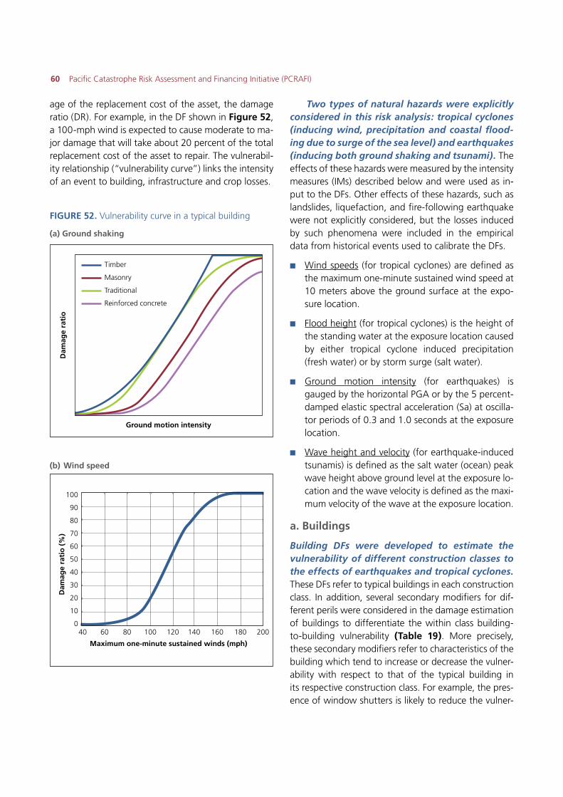
60 Pacific Catastrophe Risk Assessment and Financing Initiative (PCRAFI)
age of the replacement cost of the asset, the damage ratio (DR). For example, in the DF shown in Figure 52, a 100-mph wind is expected to cause moderate to ma-jor damage that will take about 20 percent of the total replacement cost of the asset to repair. The vulnerabil-ity relationship (“vulnerability curve”) links the intensity of an event to building, infrastructure and crop losses.
(b) Wind speed
Two types of natural hazards were explicitly considered in this risk analysis: tropical cyclones (inducing wind, precipitation and coastal flood-ing due to surge of the sea level) and earthquakes (inducing both ground shaking and tsunami). The effects of these hazards were measured by the intensity measures (IMs) described below and were used as in-put to the DFs. Other effects of these hazards, such as landslides, liquefaction, and fire-following earthquake were not explicitly considered, but the losses induced by such phenomena were included in the empirical data from historical events used to calibrate the DFs.
�� Wind speeds (for tropical cyclones) are defined as the maximum one-minute sustained wind speed at 10 meters above the ground surface at the expo-sure location.
�� Flood height (for tropical cyclones) is the height of the standing water at the exposure location caused by either tropical cyclone induced precipitation (fresh water) or by storm surge (salt water).
�� Ground motion intensity (for earthquakes) is gauged by the horizontal PGA or by the 5 percent-damped elastic spectral acceleration (Sa) at oscilla-tor periods of 0.3 and 1.0 seconds at the exposure location.
�� Wave height and velocity (for earthquake-induced tsunamis) is defined as the salt water (ocean) peak wave height above ground level at the exposure lo-cation and the wave velocity is defined as the maxi-mum velocity of the wave at the exposure location.
a. Buildings
Building DFs were developed to estimate the vulnerability of different construction classes to the effects of earthquakes and tropical cyclones. These DFs refer to typical buildings in each construction class. In addition, several secondary modifiers for dif-ferent perils were considered in the damage estimation of buildings to differentiate the within class building-to-building vulnerability (Table 19). More precisely, these secondary modifiers refer to characteristics of the building which tend to increase or decrease the vulner-ability with respect to that of the typical building in its respective construction class. For example, the pres-ence of window shutters is likely to reduce the vulner-
FIGURE 52. Vulnerability curve in a typical building
(a) Ground shaking
Timber
Masonry
Traditional
Reinforced concrete
Ground motion intensity
Maximum one-minute sustained winds (mph)
Dam
age
rati
oD
amag
e ra
tio
(%
)
100
90
80
70
60
50
40
30
20
10
040 60 80 100 120 140 160 180 200
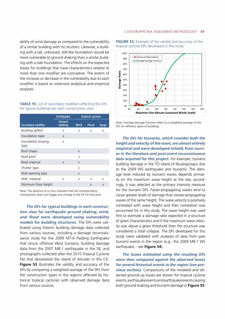
CATASTROPHE RISK ASSESSMENT METHODOLOGY 61
ability of wind damage as compared to the vulnerability of a similar building with no shutters. Likewise, a build-ing with a tall, unbraced, stilt-like foundation would be more vulnerable to ground shaking than a similar build-ing with a slab foundation. The effects on the expected losses for buildings that have characteristics related to more than one modifier are cumulative. The extent of the increase or decrease in the vulnerability due to each modifier is based on extensive analytical and empirical analyses.
TABLE 19. List of secondary modifiers affecting the DFs for typical buildings per each construction class
Secondary modifier
Earthquake Tropical cyclone
Ground shaking Wind Flood Surge
Building deflect x x x x
Foundation type x
Foundation bracing type
x
Roof shape x
Roof pitch x
Roof material x x
Shutter type x
Wall opening type x
Wall material x x x x
Minimum floor height x x
Note: The absence of a cross indicates that the corresponding characteristic does not trigger any change in the DF for that peril.
The DFs for typical buildings in each construc-tion class for earthquake ground shaking, wind, and flood were developed using vulnerability models for building structures. The DFs were cali-brated using historic building damage data collected from various sources, including a damage reconnais-sance study for the 2009 M7.6 Padang Earthquake that struck offshore West Sumatra, building damage data from the 2007 M8.1 earthquake in the SB, and photographs collected after the 2010 Tropical Cyclone Pat that devastated the island of Aitutaki in the CK. Figure 53 illustrates the validity and accuracy of the DFs by comparing a weighted average of the DFs from the construction types in the regions affected by his-torical tropical cyclones with observed damage data from various sources.
FIGURE 53. Example of the validity and accuracy of the tropical cyclone DFs developed in this study
Note: Average damage function refers to a weighted average of the DFs for different types of buildings.
The DFs for tsunamis, which consider both the height and velocity of the wave, are almost entirely empirical and were developed initially from sourc-es in the literature and post-event reconnaissance data acquired for this project. For example, tsunami building damage in the TO island of Niuatoputapu due to the 2009 WS earthquake and tsunami). The dam-age level induced by tsunami waves depends primar-ily on the maximum wave height at the site; accord-ingly, it was selected as the primary intensity measure for the tsunami DFs. Faster-propagating waves tend to cause greater levels of damage than slower-propagating waves of the same height. The wave velocity is positively correlated with wave height and their correlation was accounted for in this study. The wave height was used first to estimate a damage ratio expected in a structure of given characteristics and if the maximum wave veloc-ity was above a given threshold then the structure was considered a total collapse. The DFs developed for this study were validated with analyses of data from past tsunami events in the region (e.g., the 2009 M8.1 WS earthquake – see Figure 54).
The losses estimated using the resulting DFs were then compared against the observed losses for several historical events in the region (see pre-vious section). Comparisons of the modeled and ob-served ground-up losses are shown for tropical cyclone events, earthquake events and earthquake events causing both ground shaking and tsunami damage in Figure 55.
0%
10%
20%
30%
40%
50%
60%
70%
80%
90%
100%
40 60 80 100 120 140 160 180 200
Dam
age
Ratio
Maximim One-Minute Sustained Winds (mph)
Historical ObservationsAverage Damage Function
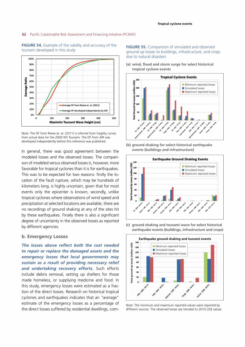
62 Pacific Catastrophe Risk Assessment and Financing Initiative (PCRAFI)
In general, there was good agreement between the modeled losses and the observed losses. The compari-son of modeled versus observed losses is, however, more favorable for tropical cyclones than it is for earthquakes. This was to be expected for two reasons: firstly the lo-cation of the fault rupture, which may be hundreds of kilometers long, is highly uncertain, given that for most events only the epicenter is known; secondly, unlike tropical cyclones where observations of wind speed and precipitation at selected locations are available, there are no recordings of ground shaking at any of the sites hit by these earthquakes. Finally there is also a significant degree of uncertainty in the observed losses as reported by different agencies.
b. Emergency Losses
The losses above reflect both the cost needed to repair or replace the damaged assets and the emergency losses that local governments may sustain as a result of providing necessary relief and undertaking recovery efforts. Such efforts include debris removal, setting up shelters for those made homeless, or supplying medicine and food. In this study, emergency losses were estimated as a frac-tion of the direct losses. Research on historical tropical cyclones and earthquakes indicates that an “average” estimate of the emergency losses as a percentage of the direct losses suffered by residential dwellings, com-
FIGURE 54. Example of the validity and accuracy of the tsunami developed in this study
Note: The DF from Reese et. al. (2011) is inferred from fragility curves from actual data for the 2009 WS Tsunami. The DF from AIR was developed independently before this reference was published.
FIGURE 55. Comparison of simulated and observed ground-up losses to buildings, infrastructure, and crops due to natural disasters
(a) wind, flood and storm surge for select historical tropical cyclone events
(b) ground shaking for select historical earthquake events (buildings and infrastructure)
(c) ground shaking and tsunami wave for select historical earthquake events (buildings, infrastructure and crops)
Note: The minimum and maximum reported values were reported by different sources. The observed losses are trended to 2010 US$ values.
Earthquake ground shaking and tsunami events
Tota
l gro
un
d-u
p lo
sses
(m
illio
n U
S$)
� Minimum reported losses� Simulated losses� Maximum reported losses
� Minimum reported losses� Simulated losses� Maximum reported losses
Tropical cyclone events
� Minimum reported losses� Simulated losses� Maximum reported losses
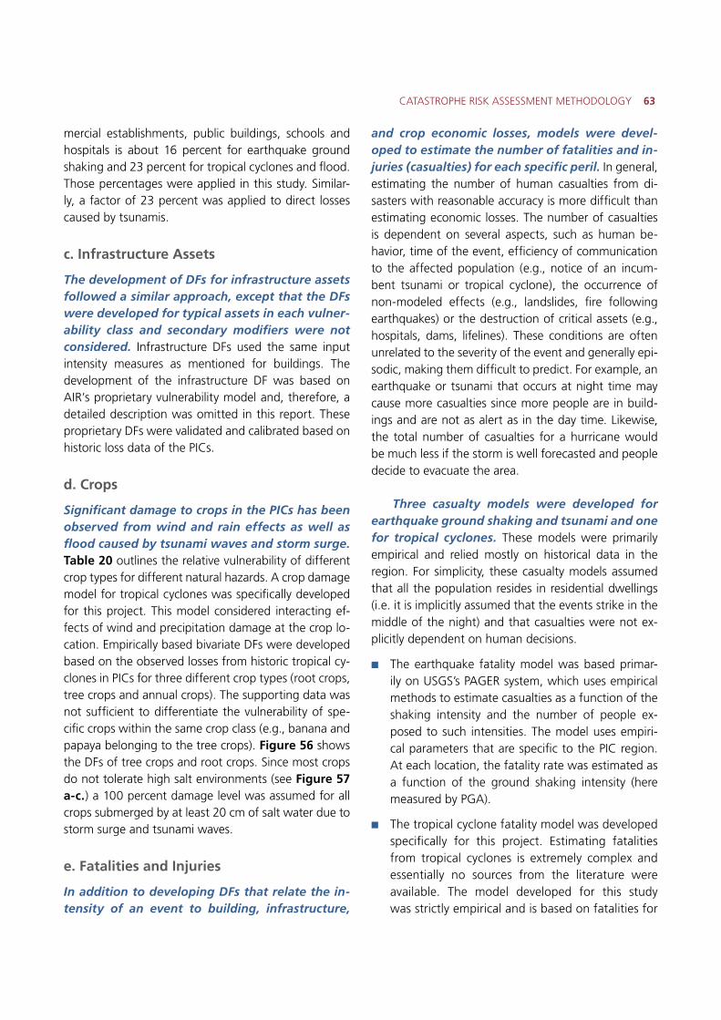
CATASTROPHE RISK ASSESSMENT METHODOLOGY 63
mercial establishments, public buildings, schools and hospitals is about 16 percent for earthquake ground shaking and 23 percent for tropical cyclones and flood. Those percentages were applied in this study. Similar-ly, a factor of 23 percent was applied to direct losses caused by tsunamis.
c. Infrastructure Assets
The development of DFs for infrastructure assets followed a similar approach, except that the DFs were developed for typical assets in each vulner-ability class and secondary modifiers were not considered. Infrastructure DFs used the same input intensity measures as mentioned for buildings. The development of the infrastructure DF was based on AIR’s proprietary vulnerability model and, therefore, a detailed description was omitted in this report. These proprietary DFs were validated and calibrated based on historic loss data of the PICs.
d. Crops
Significant damage to crops in the PICs has been observed from wind and rain effects as well as flood caused by tsunami waves and storm surge. Table 20 outlines the relative vulnerability of different crop types for different natural hazards. A crop damage model for tropical cyclones was specifically developed for this project. This model considered interacting ef-fects of wind and precipitation damage at the crop lo-cation. Empirically based bivariate DFs were developed based on the observed losses from historic tropical cy-clones in PICs for three different crop types (root crops, tree crops and annual crops). The supporting data was not sufficient to differentiate the vulnerability of spe-cific crops within the same crop class (e.g., banana and papaya belonging to the tree crops). Figure 56 shows the DFs of tree crops and root crops. Since most crops do not tolerate high salt environments (see Figure 57 a-c.) a 100 percent damage level was assumed for all crops submerged by at least 20 cm of salt water due to storm surge and tsunami waves.
e. Fatalities and Injuries
In addition to developing DFs that relate the in-tensity of an event to building, infrastructure,
and crop economic losses, models were devel-oped to estimate the number of fatalities and in-juries (casualties) for each specific peril. In general, estimating the number of human casualties from di-sasters with reasonable accuracy is more difficult than estimating economic losses. The number of casualties is dependent on several aspects, such as human be-havior, time of the event, efficiency of communication to the affected population (e.g., notice of an incum-bent tsunami or tropical cyclone), the occurrence of non-modeled effects (e.g., landslides, fire following earthquakes) or the destruction of critical assets (e.g., hospitals, dams, lifelines). These conditions are often unrelated to the severity of the event and generally epi-sodic, making them difficult to predict. For example, an earthquake or tsunami that occurs at night time may cause more casualties since more people are in build-ings and are not as alert as in the day time. Likewise, the total number of casualties for a hurricane would be much less if the storm is well forecasted and people decide to evacuate the area.
Three casualty models were developed for earthquake ground shaking and tsunami and one for tropical cyclones. These models were primarily empirical and relied mostly on historical data in the region. For simplicity, these casualty models assumed that all the population resides in residential dwellings (i.e. it is implicitly assumed that the events strike in the middle of the night) and that casualties were not ex-plicitly dependent on human decisions.
�� The earthquake fatality model was based primar-ily on USGS’s PAGER system, which uses empirical methods to estimate casualties as a function of the shaking intensity and the number of people ex-posed to such intensities. The model uses empiri-cal parameters that are specific to the PIC region. At each location, the fatality rate was estimated as a function of the ground shaking intensity (here measured by PGA).
�� The tropical cyclone fatality model was developed specifically for this project. Estimating fatalities from tropical cyclones is extremely complex and essentially no sources from the literature were available. The model developed for this study was strictly empirical and is based on fatalities for
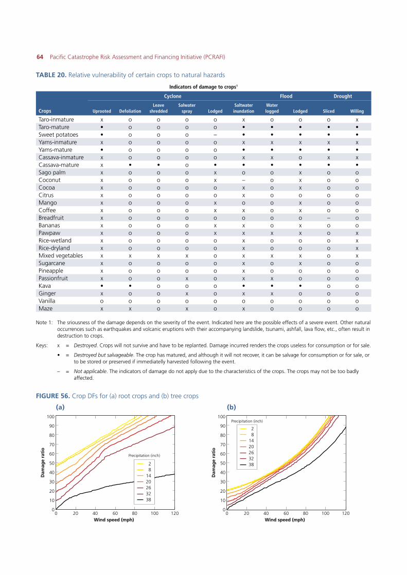
64 Pacific Catastrophe Risk Assessment and Financing Initiative (PCRAFI)
Indicators of damage to crops1
Crops
Cyclone Flood Drought
Uprooted DefoliationLeave
shreddedSalwater
spray LodgedSaltwater
inundationWater logged Lodged Sliced Willing
Taro-inmature x o o o o x o o o xTaro-mature • o o o o • • • • •Sweet potatoes • o o o – • • • • •Yams-inmature x o o o o x x x x xYams-mature • o o o o • • • • •Cassava-inmature x o o o o x x o x xCassava-mature x • • o • • • • • •Sago palm x o o o x o o x o oCoconut x o o o x – o x o oCocoa x o o o o x o x o oCitrus x o o o o x o o o oMango x o o o x o o x o oCoffee x o o o x x o x o oBreadfruit x o o o o o o o – oBananas x o o o x x o x o oPawpaw x o o o x x x x o xRice-wetland x o o o o x o o o xRice-dryland x o o o o x o o o xMixed vegetables x x x x o x x x o xSugarcane x o o o o x o x o oPineapple x o o o o x o o o oPassionfruit x o o x o x x o o oKava • • o o o • • • o oGinger x o o x o x x o o oVanilla o o o o o o o o o oMaze x x o x o x o o o o
Note 1: The sriousness of the damage depends on the severity of the event. Indicated here are the possible effects of a severe event. Other natural occurrences such as earthquakes and volcanic eruptions with their accompanying landslide, tsunami, ashfall, lava flow, etc., often result in destruction to crops.
Keys: x = Destroyed. Crops will not survive and have to be replanted. Damage incurred renders the crops useless for consumption or for sale.
• = Destroyed but salvageable. The crop has matured, and although it will not recover, it can be salvage for consumption or for sale, or to be stored or preserved if immediatelly harvested following the event.
– = Not applicable. The indicators of damage do not apply due to the characteristics of the crops. The crops may not be too badly affected.
TABLE 20. Relative vulnerability of certain crops to natural hazards
FIGURE 56. Crop DFs for (a) root crops and (b) tree crops
(a) (b)
28
1420263238
28
1420263238
100
90
80
70
60
50
40
30
20
10
0
100
90
80
70
60
50
40
30
20
10
0
Dam
age
rati
o
Dam
age
rati
o
Wind speed (mph) Wind speed (mph)20 200 040 4060 6080 80100 100120 120
Precipitation (inch)
Precipitation (inch)
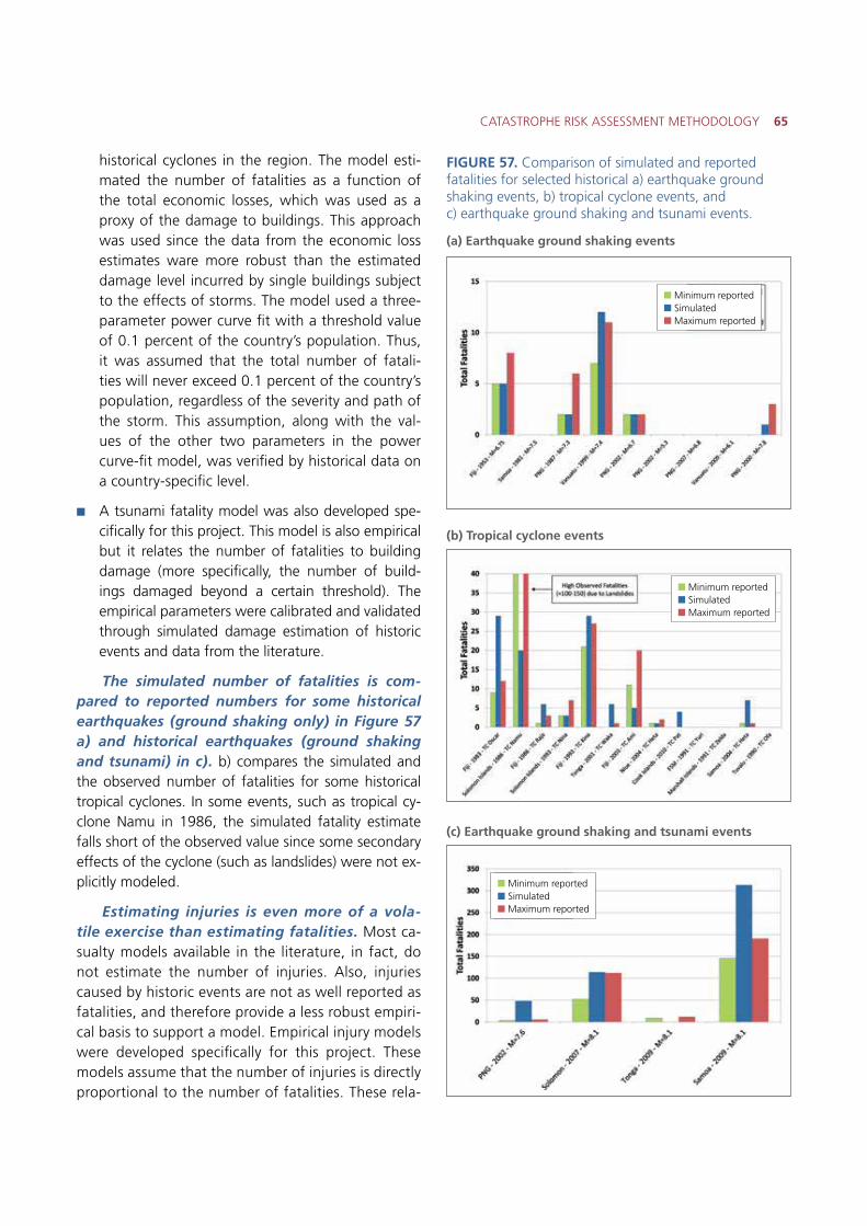
CATASTROPHE RISK ASSESSMENT METHODOLOGY 65
historical cyclones in the region. The model esti-mated the number of fatalities as a function of the total economic losses, which was used as a proxy of the damage to buildings. This approach was used since the data from the economic loss estimates ware more robust than the estimated damage level incurred by single buildings subject to the effects of storms. The model used a three-parameter power curve fit with a threshold value of 0.1 percent of the country’s population. Thus, it was assumed that the total number of fatali-ties will never exceed 0.1 percent of the country’s population, regardless of the severity and path of the storm. This assumption, along with the val-ues of the other two parameters in the power curve-fit model, was verified by historical data on a country-specific level.
�� A tsunami fatality model was also developed spe-cifically for this project. This model is also empirical but it relates the number of fatalities to building damage (more specifically, the number of build-ings damaged beyond a certain threshold). The empirical parameters were calibrated and validated through simulated damage estimation of historic events and data from the literature.
The simulated number of fatalities is com-pared to reported numbers for some historical earthquakes (ground shaking only) in Figure 57 a) and historical earthquakes (ground shaking and tsunami) in c). b) compares the simulated and the observed number of fatalities for some historical tropical cyclones. In some events, such as tropical cy-clone Namu in 1986, the simulated fatality estimate falls short of the observed value since some secondary effects of the cyclone (such as landslides) were not ex-plicitly modeled.
Estimating injuries is even more of a vola-tile exercise than estimating fatalities. Most ca-sualty models available in the literature, in fact, do not estimate the number of injuries. Also, injuries caused by historic events are not as well reported as fatalities, and therefore provide a less robust empiri-cal basis to support a model. Empirical injury models were developed specifically for this project. These models assume that the number of injuries is directly proportional to the number of fatalities. These rela-
FIGURE 57. Comparison of simulated and reported fatalities for selected historical a) earthquake ground shaking events, b) tropical cyclone events, and c) earthquake ground shaking and tsunami events.
(a) Earthquake ground shaking events
(b) Tropical cyclone events
(c) Earthquake ground shaking and tsunami events
� Minimum reported� Simulated� Maximum reported
� Minimum reported� Simulated� Maximum reported
� Minimum reported� Simulated� Maximum reported
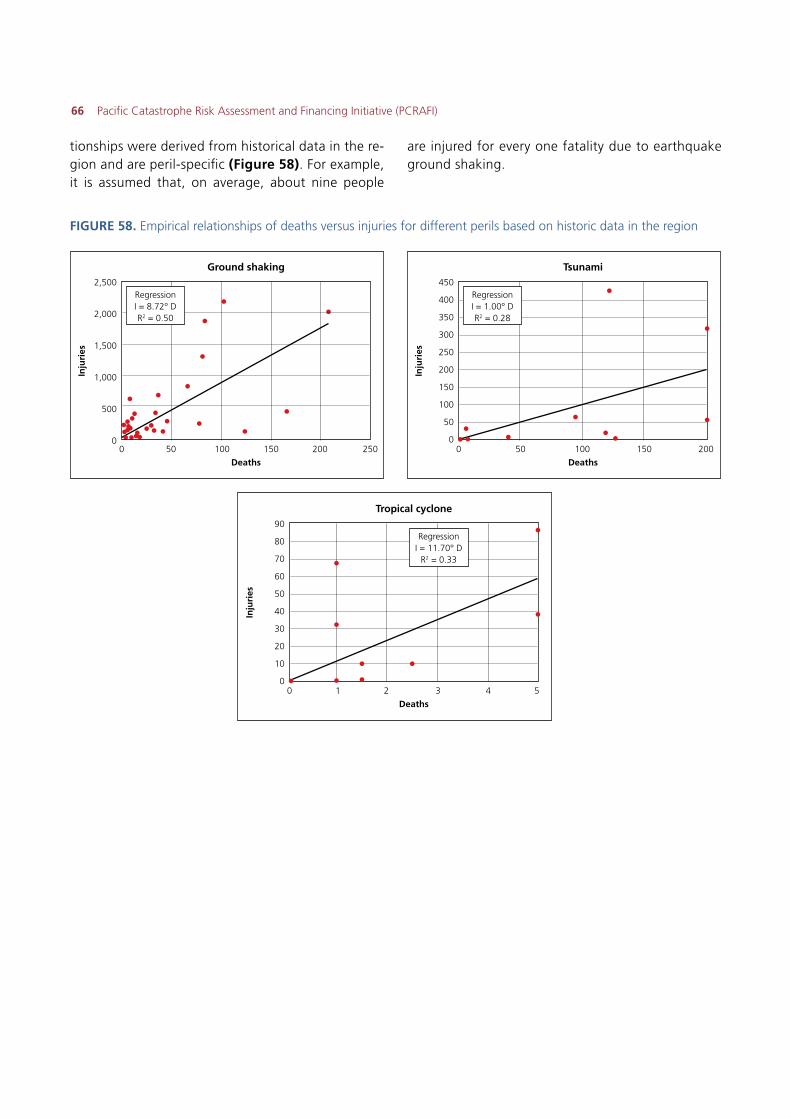
66 Pacific Catastrophe Risk Assessment and Financing Initiative (PCRAFI)
tionships were derived from historical data in the re-gion and are peril-specific (Figure 58). For example, it is assumed that, on average, about nine people
are injured for every one fatality due to earthquake ground shaking.
FIGURE 58. Empirical relationships of deaths versus injuries for different perils based on historic data in the region
2,500
2,000
1,500
1,000
500
0
450
400
350
300
250
200
150
100
50
0
90
80
70
60
50
40
30
20
10
0
0 0
0
50 50
1
100 100
2
150 150
3 4
200 200
5
250
Inju
ries
Inju
ries
Inju
ries
Deaths Deaths
Deaths
Ground shaking Tsunami
Tropical cyclone
RegressionI = 8.72° DR2 = 0.50
RegressionI = 1.00° DR2 = 0.28
RegressionI = 11.70° D
R2 = 0.33
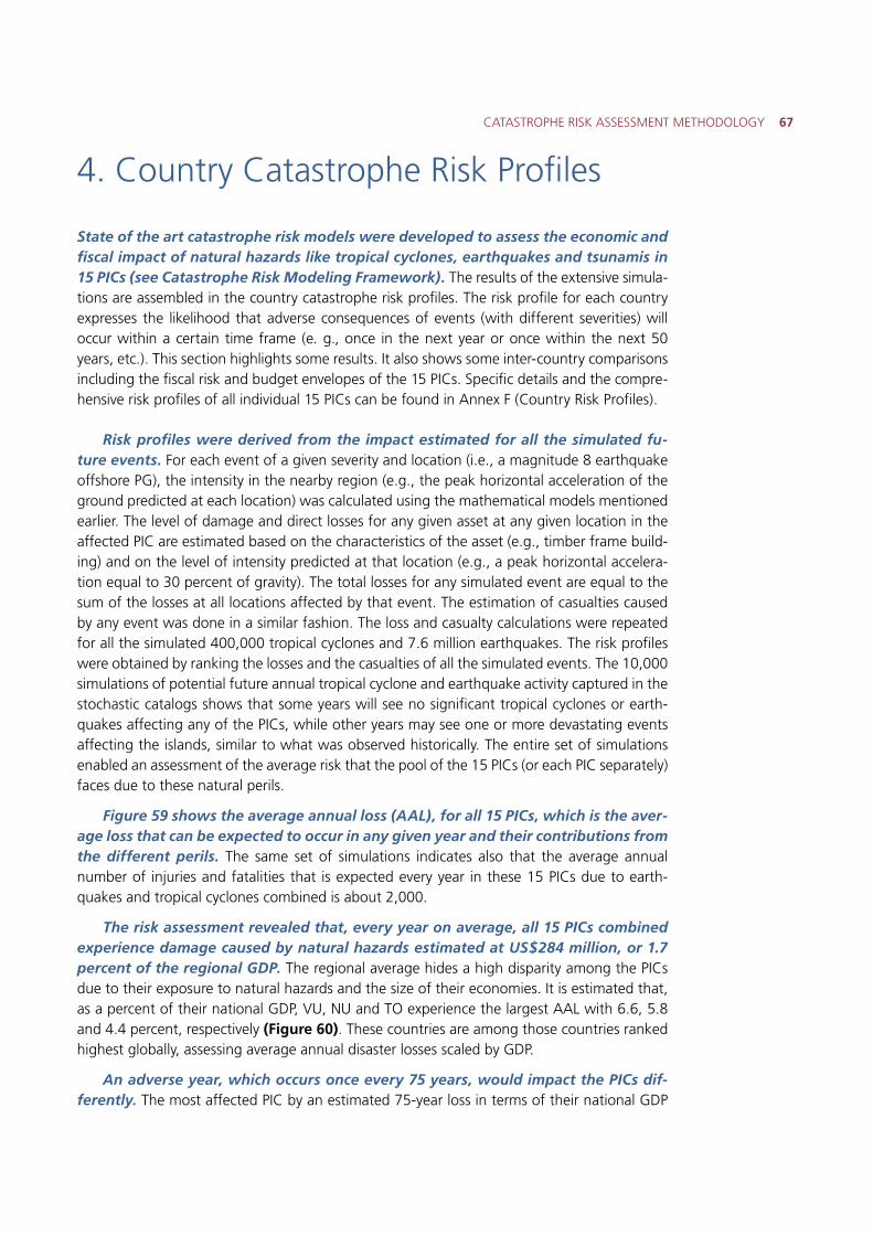
CATASTROPHE RISK ASSESSMENT METHODOLOGY 67
4. Country Catastrophe Risk Profiles
State of the art catastrophe risk models were developed to assess the economic and fiscal impact of natural hazards like tropical cyclones, earthquakes and tsunamis in 15 PICs (see Catastrophe Risk Modeling Framework). The results of the extensive simula-tions are assembled in the country catastrophe risk profiles. The risk profile for each country expresses the likelihood that adverse consequences of events (with different severities) will occur within a certain time frame (e. g., once in the next year or once within the next 50 years, etc.). This section highlights some results. It also shows some inter-country comparisons including the fiscal risk and budget envelopes of the 15 PICs. Specific details and the compre-hensive risk profiles of all individual 15 PICs can be found in Annex F (Country Risk Profiles).
Risk profiles were derived from the impact estimated for all the simulated fu-ture events. For each event of a given severity and location (i.e., a magnitude 8 earthquake offshore PG), the intensity in the nearby region (e.g., the peak horizontal acceleration of the ground predicted at each location) was calculated using the mathematical models mentioned earlier. The level of damage and direct losses for any given asset at any given location in the affected PIC are estimated based on the characteristics of the asset (e.g., timber frame build-ing) and on the level of intensity predicted at that location (e.g., a peak horizontal accelera-tion equal to 30 percent of gravity). The total losses for any simulated event are equal to the sum of the losses at all locations affected by that event. The estimation of casualties caused by any event was done in a similar fashion. The loss and casualty calculations were repeated for all the simulated 400,000 tropical cyclones and 7.6 million earthquakes. The risk profiles were obtained by ranking the losses and the casualties of all the simulated events. The 10,000 simulations of potential future annual tropical cyclone and earthquake activity captured in the stochastic catalogs shows that some years will see no significant tropical cyclones or earth-quakes affecting any of the PICs, while other years may see one or more devastating events affecting the islands, similar to what was observed historically. The entire set of simulations enabled an assessment of the average risk that the pool of the 15 PICs (or each PIC separately) faces due to these natural perils.
Figure 59 shows the average annual loss (AAL), for all 15 PICs, which is the aver-age loss that can be expected to occur in any given year and their contributions from the different perils. The same set of simulations indicates also that the average annual number of injuries and fatalities that is expected every year in these 15 PICs due to earth-quakes and tropical cyclones combined is about 2,000.
The risk assessment revealed that, every year on average, all 15 PICs combined experience damage caused by natural hazards estimated at US$284 million, or 1.7 percent of the regional GDP. The regional average hides a high disparity among the PICs due to their exposure to natural hazards and the size of their economies. It is estimated that, as a percent of their national GDP, VU, NU and TO experience the largest AAL with 6.6, 5.8 and 4.4 percent, respectively (Figure 60). These countries are among those countries ranked highest globally, assessing average annual disaster losses scaled by GDP.
An adverse year, which occurs once every 75 years, would impact the PICs dif-ferently. The most affected PIC by an estimated 75-year loss in terms of their national GDP
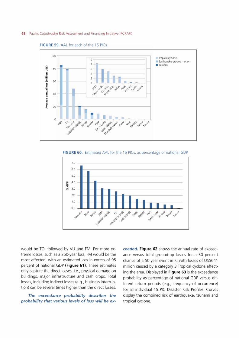
68 Pacific Catastrophe Risk Assessment and Financing Initiative (PCRAFI)
100
80
60
40
20
0
10
8
6
4
2
0
Ave
rag
e an
nu
al lo
ss (
mill
ion
US$
)
� Tropical cyclone� Earthquake ground motion� Tsunami
PNG Fij
i
Vanu
atu
Solom
on Is
lands
Tong
a
Sam
oa FSM
Timor
-Leste
Timor
-Leste
Cook I
s.
Mar
shall
Is.
FSM
Cook I
sland
s
Mar
shall
Islan
dsPa
lau
Palau
Niue
Niue
Kiribat
i
Kiribat
i
Tuva
lu
Tuva
lu
Nauru
Nauru
FIGURE 59. AAL for each of the 15 PICs
FIGURE 60. Estimated AAL for the 15 PICs, as percentage of national GDP
Vanu
atu
Solom
on Is
lands
Palau
Kiribat
i
Tong
a
Mar
shall
Islan
dsPN
GNau
ruNiue Fij
i
Sam
oa
Tuva
luFS
M
Cook I
sland
s
Timor
-Leste
7.0
6.0
5.0
4.0
3.0
2/0
1.0
0.0
% G
DP
would be TO, followed by VU and FM. For more ex-treme losses, such as a 250-year loss, FM would be the most affected, with an estimated loss in excess of 95 percent of national GDP (Figure 61). These estimates only capture the direct losses, i.e., physical damage on buildings, major infrastructure and cash crops. Total losses, including indirect losses (e.g., business interrup-tion) can be several times higher than the direct losses.
The exceedance probability describes the probability that various levels of loss will be ex-
ceeded. Figure 62 shows the annual rate of exceed-ance versus total ground-up losses for a 50 percent chance of a 50 year event in FJ with losses of US$641 million caused by a category 3 Tropical cyclone affect-ing the area. Displayed in Figure 63 is the exceedance probability as percentage of national GDP versus dif-ferent return periods (e.g., frequency of occurrence) for all individual 15 PIC Disaster Risk Profiles. Curves display the combined risk of earthquake, tsunami and tropical cyclone.
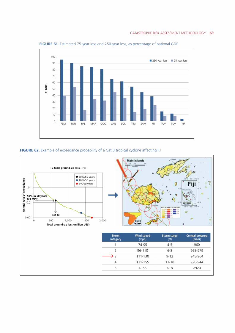
CATASTROPHE RISK ASSESSMENT METHODOLOGY 69
� 250 year loss � 25 year loss
KIRFSM TON PAL MAR COO VAN SOL TIM SAM FIJ TUV TUV
100
90
80
70
60
50
40
30
20
10
0
1
0.1
0.01
0.001
% G
DP
An
nu
al r
ate
of
exce
edan
ce
Total ground-up loss (million US$)
TC total ground-up loss – Fiji
FIGURE 61. Estimated 75-year loss and 250-year loss, as percentage of national GDP
FIGURE 62. Example of exceedance probability of a Cat 3 tropical cyclone affecting FJ
0 500
641 M
1,000 1,500 2,000
50%/50 years 10%/50 years 5%/50 years
50% in 50 years(73 MPR)
Stormcategory
Wind speed(mph)
Storm surge(ft)
Central pressure (mbar)
1 74-95 4-5 960
2 96-110 6-8 965-979
3 111-130 9-12 945-964
4 131-155 13-18 920-944
5 >155 >18 <920
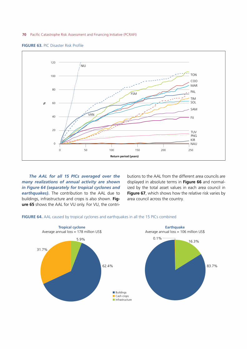
70 Pacific Catastrophe Risk Assessment and Financing Initiative (PCRAFI)
FIGURE 63. PIC Disaster Risk Profile
120
100
80
60
40
20
0
Return period (years)
%
0 50 100 150 200 250
NIU
FSM
TON
COOMAR
PAL
TIMSOL
SAM
FIJ
KIRNAU
PNGTUV
VAN
The AAL for all 15 PICs averaged over the many realizations of annual activity are shown in Figure 64 (separately for tropical cyclones and earthquakes). The contribution to the AAL due to buildings, infrastructure and crops is also shown. Fig-ure 65 shows the AAL for VU only. For VU, the contri-
butions to the AAL from the different area councils are displayed in absolute terms in Figure 66 and normal-ized by the total asset values in each area council in Figure 67, which shows how the relative risk varies by area council across the country.
FIGURE 64. AAL caused by tropical cyclones and earthquakes in all the 15 PICs combined
5.9% 16.3%
31.7%
0.1%
62.4% 83.7%
Tropical cycloneAverage annual loss = 178 million US$
EarthquakeAverage annual loss = 106 million US$
� Buildings� Cash crops� Infrastructure
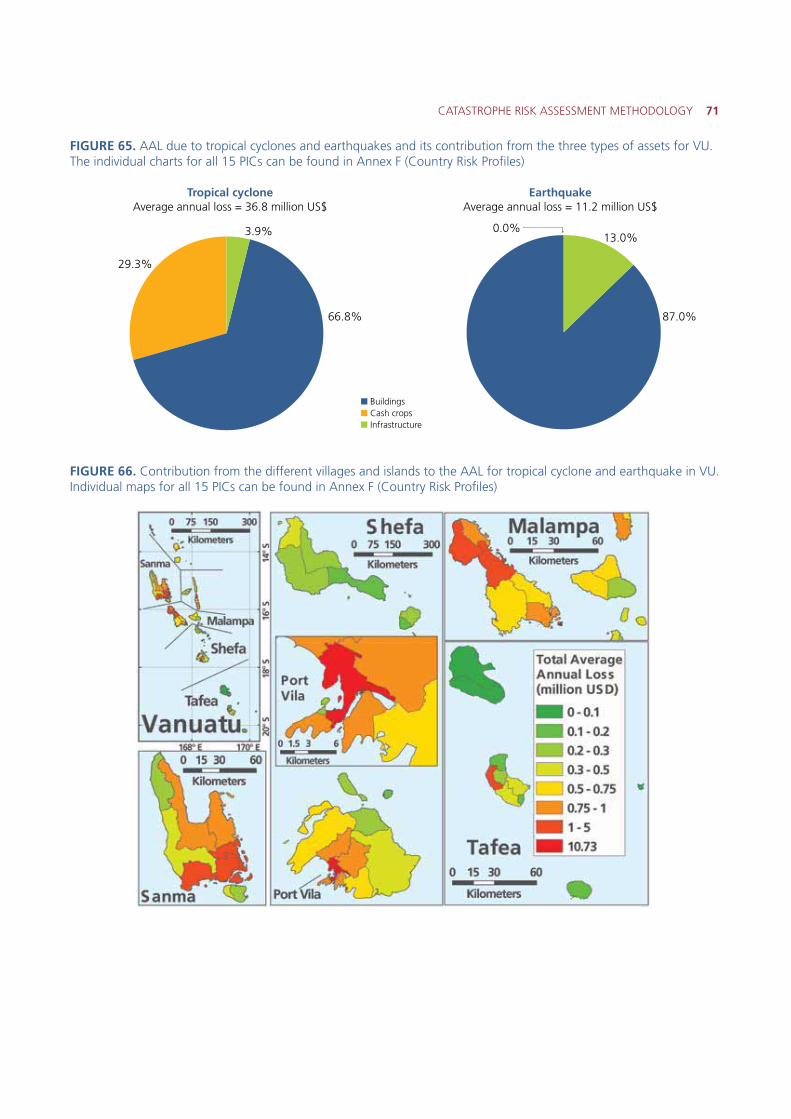
CATASTROPHE RISK ASSESSMENT METHODOLOGY 71
FIGURE 65. AAL due to tropical cyclones and earthquakes and its contribution from the three types of assets for VU. The individual charts for all 15 PICs can be found in Annex F (Country Risk Profiles)
3.9% 13.0%
29.3%
0.0%
66.8% 87.0%
Tropical cycloneAverage annual loss = 36.8 million US$
EarthquakeAverage annual loss = 11.2 million US$
� Buildings� Cash crops� Infrastructure
FIGURE 66. Contribution from the different villages and islands to the AAL for tropical cyclone and earthquake in VU. Individual maps for all 15 PICs can be found in Annex F (Country Risk Profiles)
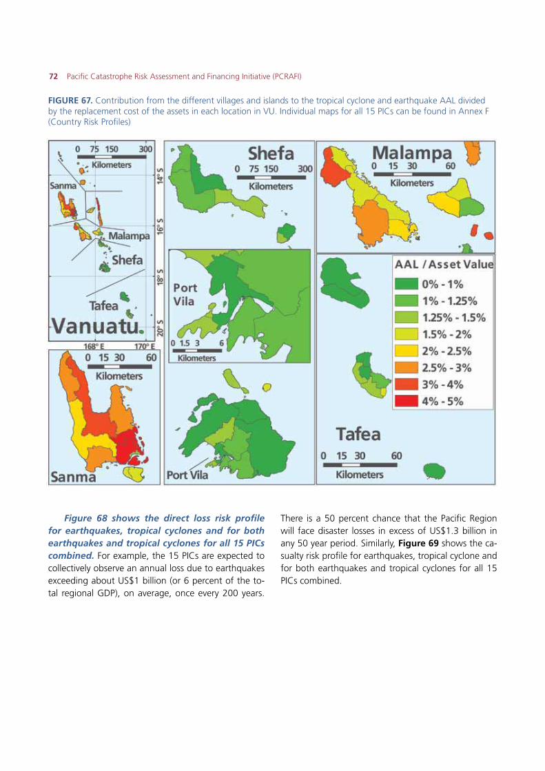
72 Pacific Catastrophe Risk Assessment and Financing Initiative (PCRAFI)
FIGURE 67. Contribution from the different villages and islands to the tropical cyclone and earthquake AAL divided by the replacement cost of the assets in each location in VU. Individual maps for all 15 PICs can be found in Annex F (Country Risk Profiles)
Figure 68 shows the direct loss risk profile for earthquakes, tropical cyclones and for both earthquakes and tropical cyclones for all 15 PICs combined. For example, the 15 PICs are expected to collectively observe an annual loss due to earthquakes exceeding about US$1 billion (or 6 percent of the to-tal regional GDP), on average, once every 200 years.
There is a 50 percent chance that the Pacific Region will face disaster losses in excess of US$1.3 billion in any 50 year period. Similarly, Figure 69 shows the ca-sualty risk profile for earthquakes, tropical cyclone and for both earthquakes and tropical cyclones for all 15 PICs combined.
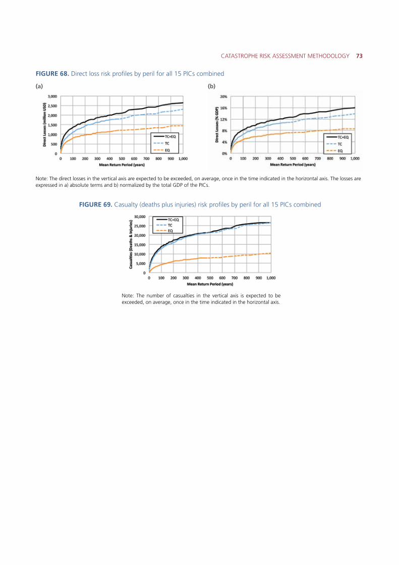
CATASTROPHE RISK ASSESSMENT METHODOLOGY 73
FIGURE 68. Direct loss risk profiles by peril for all 15 PICs combined
(a) (b)
Note: The direct losses in the vertical axis are expected to be exceeded, on average, once in the time indicated in the horizontal axis. The losses are expressed in a) absolute terms and b) normalized by the total GDP of the PICs.
FIGURE 69. Casualty (deaths plus injuries) risk profiles by peril for all 15 PICs combined
Note: The number of casualties in the vertical axis is expected to be exceeded, on average, once in the time indicated in the horizontal axis.
74 Pacific Catastrophe Risk Assessment and Financing Initiative (PCRAFI)
5. The Pacific Risk Information System (PacRIS)
The Pacific Risk Information System (PacRIS) houses the most comprehensive re-gional database of baseline exposure (buildings, infrastructure and crops) and prob-abilistic risk assessment results for all 15 PICs. The exposure database leverages remote sensing analyses, field visits, and country specific datasets to characterize buildings (residen-tial, commercial, and industrial), major infrastructure (such as roads, bridges, airports, and electricity), major crops and population. More than 530,000 buildings were digitized from very-high-resolution satellite images, representing 15 percent (or 36 percent without PG) of the estimated total number of buildings in the PICs. About 80,000 buildings and major in-frastructure were physically inspected. In addition, about 3 million buildings and other assets, mostly in rural areas, were inferred from satellite imagery.
PacRIS includes the most comprehensive regional historical hazard catalogue (115,000 earthquake and 2,500 tropical cyclone events) and historical loss data-base for major disasters, as well as country-specific hazard models that simulate earthquakes, tsunamis) and tropical cyclones. PacRIS contains risk maps showing the geographic distribution of potential losses for each PIC as well as other visualization prod-ucts of the risk assessments, which can be accessed, with appropriate authorization, through an open-source web-based platform. PacRIS enables proactive regional integration with the newly launched Open Data for Resilience Initiative (OpenDRI). OpenDRI is a ‘World Bank-wide’ initiative that seeks to support decision making by facilitating the sharing and use of information for building resilience to natural hazards in a changing climate. PCRAFI developed the Pacific GeoNode as a central web-based data and information sharing platform enabling PICs and development partners’ access to the risk information, tools and knowledge products developed under the initiative. As such, it is one of the flagships for good practice under OpenDRI.
In the next phase, PacRIS will be further built and refined by:
(I) Strengthening the capacity of technical agencies at national and regional level in its use and maintenance;
(II) Strengthening the risk information and underlying data, including the update of risk exposure databases;
(III) Strengthening the data-sharing platform at SPC/SOPAC in order to achieve expanded reach and allow access of PCRAFI data and information to the wider Pacific community; and by
(IV) Developing country risk atlases and other knowledge products to effectively communi-cate risk information to policy and decision makers.
The data and models of the PacRIS will evolve to suit the needs of its applica-tions. Therefore, the applications will drive the System’s evolution and manage-ment.
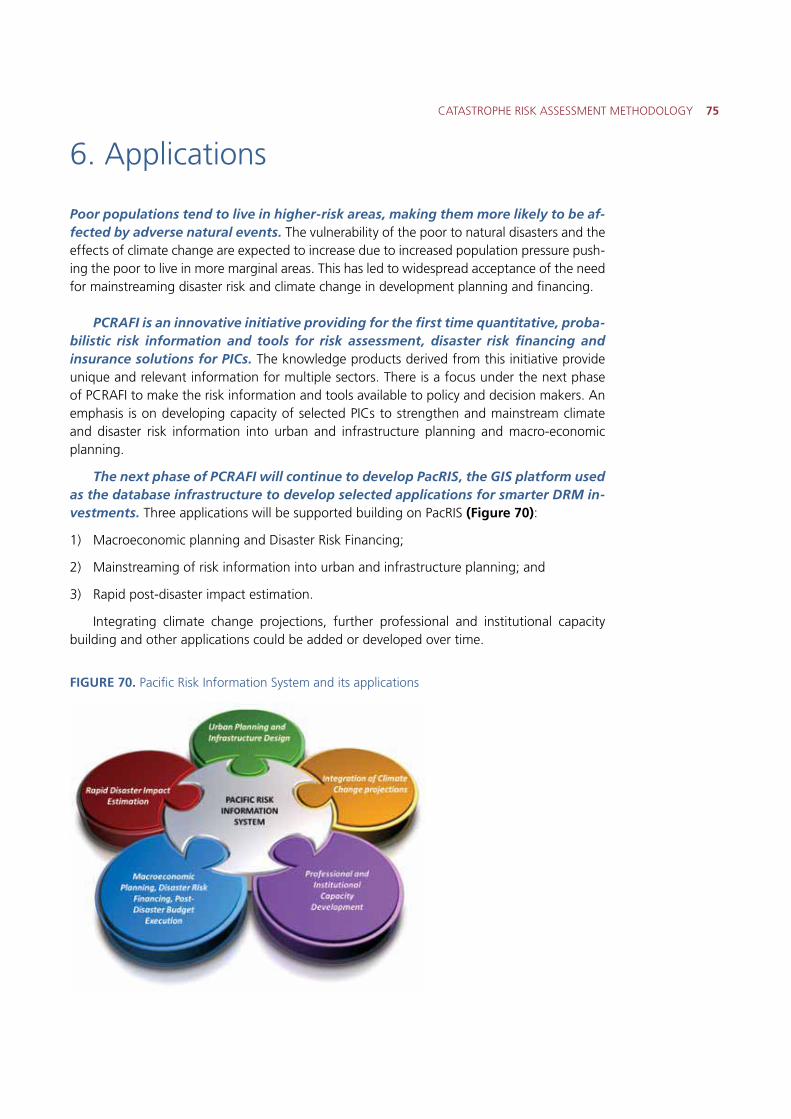
CATASTROPHE RISK ASSESSMENT METHODOLOGY 75
6. Applications
Poor populations tend to live in higher-risk areas, making them more likely to be af-fected by adverse natural events. The vulnerability of the poor to natural disasters and the effects of climate change are expected to increase due to increased population pressure push-ing the poor to live in more marginal areas. This has led to widespread acceptance of the need for mainstreaming disaster risk and climate change in development planning and financing.
PCRAFI is an innovative initiative providing for the first time quantitative, proba-bilistic risk information and tools for risk assessment, disaster risk financing and insurance solutions for PICs. The knowledge products derived from this initiative provide unique and relevant information for multiple sectors. There is a focus under the next phase of PCRAFI to make the risk information and tools available to policy and decision makers. An emphasis is on developing capacity of selected PICs to strengthen and mainstream climate and disaster risk information into urban and infrastructure planning and macro-economic planning.
The next phase of PCRAFI will continue to develop PacRIS, the GIS platform used as the database infrastructure to develop selected applications for smarter DRM in-vestments. Three applications will be supported building on PacRIS (Figure 70):
1) Macroeconomic planning and Disaster Risk Financing;
2) Mainstreaming of risk information into urban and infrastructure planning; and
3) Rapid post-disaster impact estimation.
Integrating climate change projections, further professional and institutional capacity building and other applications could be added or developed over time.
FIGURE 70. Pacific Risk Information System and its applications
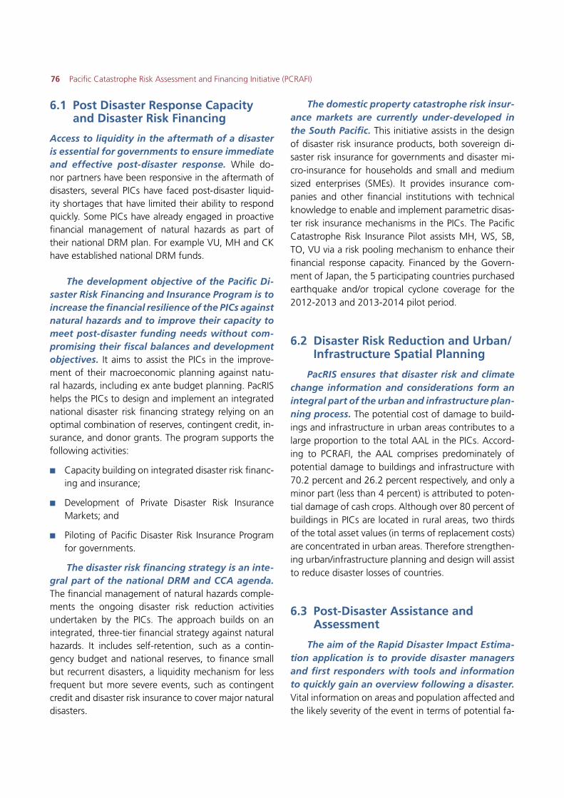
76 Pacific Catastrophe Risk Assessment and Financing Initiative (PCRAFI)
6.1 Post Disaster Response Capacity and Disaster Risk Financing
Access to liquidity in the aftermath of a disaster is essential for governments to ensure immediate and effective post-disaster response. While do-nor partners have been responsive in the aftermath of disasters, several PICs have faced post-disaster liquid-ity shortages that have limited their ability to respond quickly. Some PICs have already engaged in proactive financial management of natural hazards as part of their national DRM plan. For example VU, MH and CK have established national DRM funds.
The development objective of the Pacific Di-saster Risk Financing and Insurance Program is to increase the financial resilience of the PICs against natural hazards and to improve their capacity to meet post-disaster funding needs without com-promising their fiscal balances and development objectives. It aims to assist the PICs in the improve-ment of their macroeconomic planning against natu-ral hazards, including ex ante budget planning. PacRIS helps the PICs to design and implement an integrated national disaster risk financing strategy relying on an optimal combination of reserves, contingent credit, in-surance, and donor grants. The program supports the following activities:
�� Capacity building on integrated disaster risk financ-ing and insurance;
�� Development of Private Disaster Risk Insurance Markets; and
�� Piloting of Pacific Disaster Risk Insurance Program for governments.
The disaster risk financing strategy is an inte-gral part of the national DRM and CCA agenda. The financial management of natural hazards comple-ments the ongoing disaster risk reduction activities undertaken by the PICs. The approach builds on an integrated, three-tier financial strategy against natural hazards. It includes self-retention, such as a contin-gency budget and national reserves, to finance small but recurrent disasters, a liquidity mechanism for less frequent but more severe events, such as contingent credit and disaster risk insurance to cover major natural disasters.
The domestic property catastrophe risk insur-ance markets are currently under-developed in the South Pacific. This initiative assists in the design of disaster risk insurance products, both sovereign di-saster risk insurance for governments and disaster mi-cro-insurance for households and small and medium sized enterprises (SMEs). It provides insurance com-panies and other financial institutions with technical knowledge to enable and implement parametric disas-ter risk insurance mechanisms in the PICs. The Pacific Catastrophe Risk Insurance Pilot assists MH, WS, SB, TO, VU via a risk pooling mechanism to enhance their financial response capacity. Financed by the Govern-ment of Japan, the 5 participating countries purchased earthquake and/or tropical cyclone coverage for the 2012-2013 and 2013-2014 pilot period.
6.2 Disaster Risk Reduction and Urban/Infrastructure Spatial Planning
PacRIS ensures that disaster risk and climate change information and considerations form an integral part of the urban and infrastructure plan-ning process. The potential cost of damage to build-ings and infrastructure in urban areas contributes to a large proportion to the total AAL in the PICs. Accord-ing to PCRAFI, the AAL comprises predominately of potential damage to buildings and infrastructure with 70.2 percent and 26.2 percent respectively, and only a minor part (less than 4 percent) is attributed to poten-tial damage of cash crops. Although over 80 percent of buildings in PICs are located in rural areas, two thirds of the total asset values (in terms of replacement costs) are concentrated in urban areas. Therefore strengthen-ing urban/infrastructure planning and design will assist to reduce disaster losses of countries.
6.3 Post-Disaster Assistance and Assessment
The aim of the Rapid Disaster Impact Estima-tion application is to provide disaster managers and first responders with tools and information to quickly gain an overview following a disaster. Vital information on areas and population affected and the likely severity of the event in terms of potential fa-
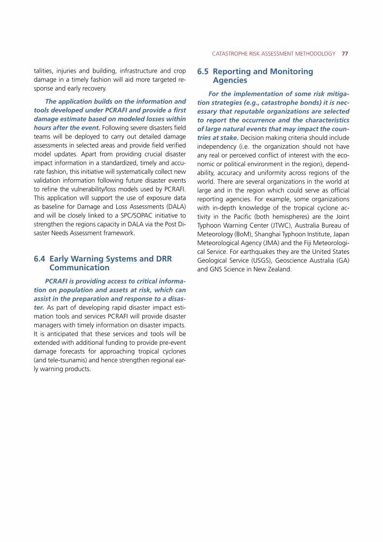
CATASTROPHE RISK ASSESSMENT METHODOLOGY 77
talities, injuries and building, infrastructure and crop damage in a timely fashion will aid more targeted re-sponse and early recovery.
The application builds on the information and tools developed under PCRAFI and provide a first damage estimate based on modeled losses within hours after the event. Following severe disasters field teams will be deployed to carry out detailed damage assessments in selected areas and provide field verified model updates. Apart from providing crucial disaster impact information in a standardized, timely and accu-rate fashion, this initiative will systematically collect new validation information following future disaster events to refine the vulnerability/loss models used by PCRAFI. This application will support the use of exposure data as baseline for Damage and Loss Assessments (DALA) and will be closely linked to a SPC/SOPAC initiative to strengthen the regions capacity in DALA via the Post Di-saster Needs Assessment framework.
6.4 Early Warning Systems and DRR Communication
PCRAFI is providing access to critical informa-tion on population and assets at risk, which can assist in the preparation and response to a disas-ter. As part of developing rapid disaster impact esti-mation tools and services PCRAFI will provide disaster managers with timely information on disaster impacts. It is anticipated that these services and tools will be extended with additional funding to provide pre-event damage forecasts for approaching tropical cyclones (and tele-tsunamis) and hence strengthen regional ear-ly warning products.
6.5 Reporting and Monitoring Agencies
For the implementation of some risk mitiga-tion strategies (e.g., catastrophe bonds) it is nec-essary that reputable organizations are selected to report the occurrence and the characteristics of large natural events that may impact the coun-tries at stake. Decision making criteria should include independency (i.e. the organization should not have any real or perceived conflict of interest with the eco-nomic or political environment in the region), depend-ability, accuracy and uniformity across regions of the world. There are several organizations in the world at large and in the region which could serve as official reporting agencies. For example, some organizations with in-depth knowledge of the tropical cyclone ac-tivity in the Pacific (both hemispheres) are the Joint Typhoon Warning Center (JTWC), Australia Bureau of Meteorology (BoM), Shanghai Typhoon Institute, Japan Meteorological Agency (JMA) and the Fiji Meteorologi-cal Service. For earthquakes they are the United States Geological Service (USGS), Geoscience Australia (GA) and GNS Science in New Zealand.
78 Pacific Catastrophe Risk Assessment and Financing Initiative (PCRAFI)
7. References
Pacific Catastrophe Risk Assessment and Financing Initiative (PCRAFI), Component 1: Hazard Data and Loss Data Collection and Management, Technical Report Submitted to the World Bank by AIR Worldwide, December 2010.
Pacific Catastrophe Risk Assessment and Financing Initiative (PCRAFI), Component 2: Expo-sure Data Collection and Management, Technical Report Submitted to the World Bank by AIR Worldwide, September 2011.
Pacific Catastrophe Risk Assessment and Financing Initiative (PCRAFI), Component 3: Country Catastrophe Risk Profiles, Technical Report Submitted to the World Bank by AIR Worldwide, December 2011.
Pacific Catastrophe Risk Assessment and Financing Initiative (PCRAFI), Component 4: Port-folio Risk Analysis Report, Technical Report Submitted to the World Bank by AIR Worldwide, November 2011.
Pacific Catastrophe Risk Assessment and Financing Initiative (PCRAFI), Catastrophic Loss Da-tabase Tool, User’s Manual Submitted to the World Bank by AIR Worldwide, December 2011.
Pacific Catastrophe Risk Assessment and Financing Initiative (PCRAFI), Risk Assessment Meth-odology, September 2011.
Pacific Catastrophe Risk Assessment and Financing Initiative (PCRAFI), Progress Brief, August 2011.
Pacific Catastrophe Risk Assessment and Financing Initiative (PCRAFI), Pacific Disaster Risk Financing and Insurance Program (PDRFIS), August 2011.
Asian Development Bank (ADB), I, Final report, TA 6496-RE: Regional Partnership for Climate Change: Adaptation and Disaster Preparedness, July 2011.
Pacific Catastrophe Risk Financing Initiative, Catastrophe Risk Assessment and Options for Regional Risk Financing; The World Bank; September 2008.
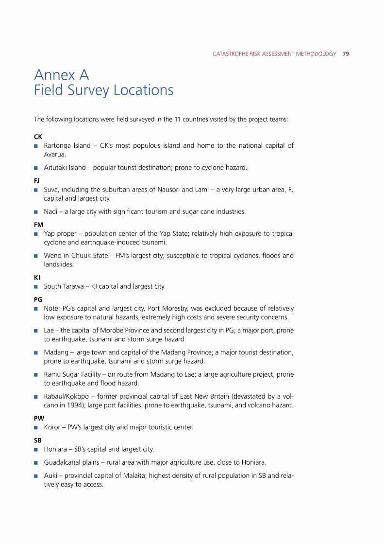
CATASTROPHE RISK ASSESSMENT METHODOLOGY 79
Annex A Field Survey Locations
The following locations were field surveyed in the 11 countries visited by the project teams:
CK�� Rartonga Island – CK’s most populous island and home to the national capital of
Avarua.
�� Aitutaki Island – popular tourist destination; prone to cyclone hazard.
FJ�� Suva, including the suburban areas of Nausori and Lami – a very large urban area, FJ
capital and largest city.
�� Nadi – a large city with significant tourism and sugar cane industries.
FM�� Yap proper – population center of the Yap State; relatively high exposure to tropical
cyclone and earthquake-induced tsunami.
�� Weno in Chuuk State – FM’s largest city; susceptible to tropical cyclones, floods and landslides.
KI�� South Tarawa – KI capital and largest city.
PG�� Note: PG’s capital and largest city, Port Moresby, was excluded because of relatively
low exposure to natural hazards, extremely high costs and severe security concerns.
�� Lae – the capital of Morobe Province and second largest city in PG; a major port, prone to earthquake, tsunami and storm surge hazard.
�� Madang – large town and capital of the Madang Province; a major tourist destination, prone to earthquake, tsunami and storm surge hazard.
�� Ramu Sugar Facility – on route from Madang to Lae; a large agriculture project, prone to earthquake and flood hazard.
�� Rabaul/Kokopo – former provincial capital of East New Britain (devastated by a vol-cano in 1994); large port facilities, prone to earthquake, tsunami, and volcano hazard.
PW�� Koror – PW’s largest city and major touristic center.
SB�� Honiara – SB’s capital and largest city.
�� Guadalcanal plains – rural area with major agriculture use, close to Honiara.
�� Auki – provincial capital of Malaita; highest density of rural population in SB and rela-tively easy to access.
80 Pacific Catastrophe Risk Assessment and Financing Initiative (PCRAFI)
�� Noro – large town in the Western Province; a major sea port and fish cannery.
�� Munda –largest settlement on the island of New Georgia in the Western Province.
�� Gizo –capital of the Western Province and SB’s second largest city.
�� Ringgi – settlement on Kolombangara Island in the New Georgia Island group.
TO�� Nuku’alofa, including other areas in Tongatapu – Nuku’alofa, TO’s capital and largest city; located on TO’s
main island of Tongatapu, prone to earthquake and tropical cyclone hazard.
TV�� Funafuti – TV’s capital and most populated atoll.
VU�� Port Vila, including suburbs and surrounding villages – VU’s capital and largest city.
�� Luganville and surrounding villages – VU’s second largest city and only other large settlement in VU be-sides Port Vila.
�� South-West Tanna Island – a major tourism/resort destination.
�� North-East Ambae Island (Lolowaï) – a rural settlement on an outer island.
WS�� Apia – WS’s capital and largest city.
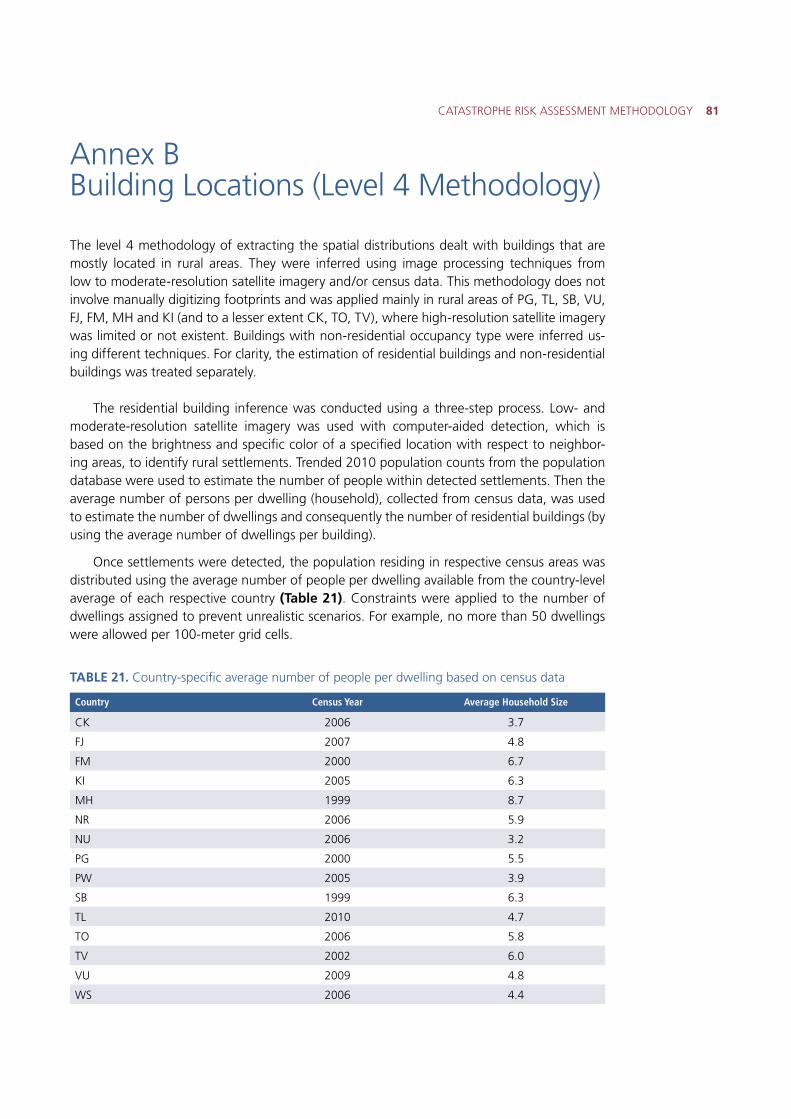
CATASTROPHE RISK ASSESSMENT METHODOLOGY 81
Annex B Building Locations (Level 4 Methodology)
The level 4 methodology of extracting the spatial distributions dealt with buildings that are mostly located in rural areas. They were inferred using image processing techniques from low to moderate-resolution satellite imagery and/or census data. This methodology does not involve manually digitizing footprints and was applied mainly in rural areas of PG, TL, SB, VU, FJ, FM, MH and KI (and to a lesser extent CK, TO, TV), where high-resolution satellite imagery was limited or not existent. Buildings with non-residential occupancy type were inferred us-ing different techniques. For clarity, the estimation of residential buildings and non-residential buildings was treated separately.
The residential building inference was conducted using a three-step process. Low- and moderate-resolution satellite imagery was used with computer-aided detection, which is based on the brightness and specific color of a specified location with respect to neighbor-ing areas, to identify rural settlements. Trended 2010 population counts from the population database were used to estimate the number of people within detected settlements. Then the average number of persons per dwelling (household), collected from census data, was used to estimate the number of dwellings and consequently the number of residential buildings (by using the average number of dwellings per building).
Once settlements were detected, the population residing in respective census areas was distributed using the average number of people per dwelling available from the country-level average of each respective country (Table 21). Constraints were applied to the number of dwellings assigned to prevent unrealistic scenarios. For example, no more than 50 dwellings were allowed per 100-meter grid cells.
TABLE 21. Country-specific average number of people per dwelling based on census data
Country Census Year Average Household Size
CK 2006 3.7
FJ 2007 4.8
FM 2000 6.7
KI 2005 6.3
MH 1999 8.7
NR 2006 5.9
NU 2006 3.2
PG 2000 5.5
PW 2005 3.9
SB 1999 6.3
TL 2010 4.7
TO 2006 5.8
TV 2002 6.0
VU 2009 4.8
WS 2006 4.4
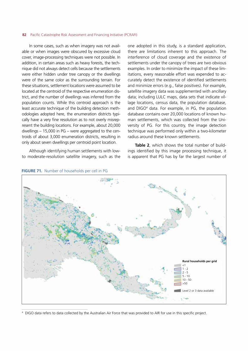
82 Pacific Catastrophe Risk Assessment and Financing Initiative (PCRAFI)
In some cases, such as when imagery was not avail-able or when images were obscured by excessive cloud cover, image-processing techniques were not possible. In addition, in certain areas such as heavy forests, the tech-nique did not always detect cells because the settlements were either hidden under tree canopy or the dwellings were of the same color as the surrounding terrain. For these situations, settlement locations were assumed to be located at the centroid of the respective enumeration dis-trict, and the number of dwellings was inferred from the population counts. While this centroid approach is the least accurate technique of the building detection meth-odologies adopted here, the enumeration districts typi-cally have a very fine resolution as to not overly misrep-resent the building locations. For example, about 20,000 dwellings – 15,000 in PG – were aggregated to the cen-troids of about 3,000 enumeration districts, resulting in only about seven dwellings per centroid point location.
Although identifying human settlements with low- to moderate-resolution satellite imagery, such as the
one adopted in this study, is a standard application, there are limitations inherent to this approach. The interference of cloud coverage and the existence of settlements under the canopy of trees are two obvious examples. In order to minimize the impact of these lim-itations, every reasonable effort was expended to ac-curately detect the existence of identified settlements and minimize errors (e.g., false positives). For example, satellite imagery data was supplemented with ancillary data; including LULC maps, data sets that indicate vil-lage locations, census data, the population database, and DIGO4 data. For example, in PG, the population database contains over 20,000 locations of known hu-man settlements, which was collected from the Uni-versity of PG. For this country, the image detection technique was performed only within a two-kilometer radius around these known settlements.
Table 2, which shows the total number of build-ings identified by this image processing technique, it is apparent that PG has by far the largest number of
4 DIGO data refers to data collected by the Australian Air Force that was provided to AIR for use in this specific project.
FIGURE 71. Number of households per cell in PG
<11 - 22 - 55 - 1010 - 50>50
Level 2 or 3 data available
Rural households per grid
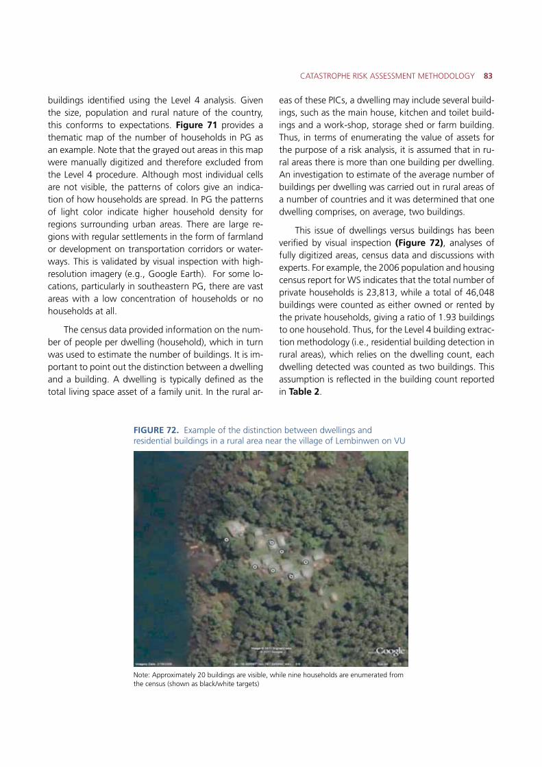
CATASTROPHE RISK ASSESSMENT METHODOLOGY 83
buildings identified using the Level 4 analysis. Given the size, population and rural nature of the country, this conforms to expectations. Figure 71 provides a thematic map of the number of households in PG as an example. Note that the grayed out areas in this map were manually digitized and therefore excluded from the Level 4 procedure. Although most individual cells are not visible, the patterns of colors give an indica-tion of how households are spread. In PG the patterns of light color indicate higher household density for regions surrounding urban areas. There are large re-gions with regular settlements in the form of farmland or development on transportation corridors or water-ways. This is validated by visual inspection with high-resolution imagery (e.g., Google Earth). For some lo-cations, particularly in southeastern PG, there are vast areas with a low concentration of households or no households at all.
The census data provided information on the num-ber of people per dwelling (household), which in turn was used to estimate the number of buildings. It is im-portant to point out the distinction between a dwelling and a building. A dwelling is typically defined as the total living space asset of a family unit. In the rural ar-
eas of these PICs, a dwelling may include several build-ings, such as the main house, kitchen and toilet build-ings and a work-shop, storage shed or farm building. Thus, in terms of enumerating the value of assets for the purpose of a risk analysis, it is assumed that in ru-ral areas there is more than one building per dwelling. An investigation to estimate of the average number of buildings per dwelling was carried out in rural areas of a number of countries and it was determined that one dwelling comprises, on average, two buildings.
This issue of dwellings versus buildings has been verified by visual inspection (Figure 72), analyses of fully digitized areas, census data and discussions with experts. For example, the 2006 population and housing census report for WS indicates that the total number of private households is 23,813, while a total of 46,048 buildings were counted as either owned or rented by the private households, giving a ratio of 1.93 buildings to one household. Thus, for the Level 4 building extrac-tion methodology (i.e., residential building detection in rural areas), which relies on the dwelling count, each dwelling detected was counted as two buildings. This assumption is reflected in the building count reported in Table 2.
FIGURE 72. Example of the distinction between dwellings and residential buildings in a rural area near the village of Lembinwen on VU
Note: Approximately 20 buildings are visible, while nine households are enumerated from the census (shown as black/white targets)
84 Pacific Catastrophe Risk Assessment and Financing Initiative (PCRAFI)
The Level 4 building inference methodology was based on census data which only enumerates residen-tial dwellings. Location and counts of non-residential buildings, including commercial, industrial and public buildings were inferred from those of residential build-ings. Data from the building field surveys, building counts from completely digitized countries (e.g., NR and NU), as well as ancillary sources (A 2007 Water-works Division Survey in the CK and the Pacific Cities Database) indicate that 80 to 97 percent of the total buildings in a given area in the PICs are used for resi-
dential purposes. For rural areas, the ratio is slightly higher, with 88 to 97 percent of the total buildings used for residential purposes. Thus, for the Level 4 building detection methodology in rural areas, extra buildings were added at random among the locations of the detected settlement cells, so that approximately 95 percent of the buildings were designated as resi-dential. For example, if 95 buildings were detected in ten settlement cells in a certain area, five non-residen-tial buildings were added in one randomly chosen cell among the ten identified.
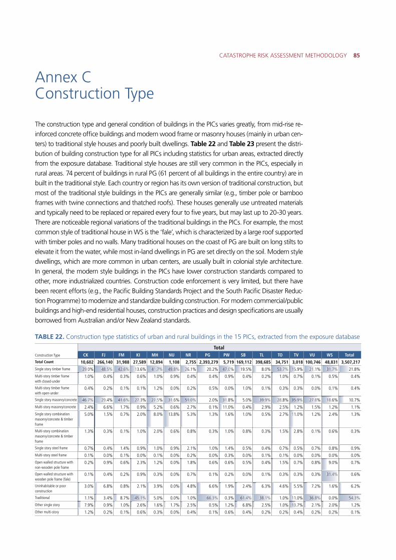
CATASTROPHE RISK ASSESSMENT METHODOLOGY 85
Annex C Construction Type
The construction type and general condition of buildings in the PICs varies greatly, from mid-rise re-inforced concrete office buildings and modern wood frame or masonry houses (mainly in urban cen-ters) to traditional style houses and poorly built dwellings. Table 22 and Table 23 present the distri-bution of building construction type for all PICs including statistics for urban areas, extracted directly from the exposure database. Traditional style houses are still very common in the PICs, especially in rural areas. 74 percent of buildings in rural PG (61 percent of all buildings in the entire country) are in built in the traditional style. Each country or region has its own version of traditional construction, but most of the traditional style buildings in the PICs are generally similar (e.g., timber pole or bamboo frames with twine connections and thatched roofs). These houses generally use untreated materials and typically need to be replaced or repaired every four to five years, but may last up to 20-30 years. There are noticeable regional variations of the traditional buildings in the PICs. For example, the most common style of traditional house in WS is the ‘fale’, which is characterized by a large roof supported with timber poles and no walls. Many traditional houses on the coast of PG are built on long stilts to elevate it from the water, while most in-land dwellings in PG are set directly on the soil. Modern style dwellings, which are more common in urban centers, are usually built in colonial style architecture. In general, the modern style buildings in the PICs have lower construction standards compared to other, more industrialized countries. Construction code enforcement is very limited, but there have been recent efforts (e.g., the Pacific Building Standards Project and the South Pacific Disaster Reduc-tion Programme) to modernize and standardize building construction. For modern commercial/public buildings and high-end residential houses, construction practices and design specifications are usually borrowed from Australian and/or New Zealand standards.
TABLE 22. Construction type statistics of urban and rural buildings in the 15 PICs, extracted from the exposure database
Construction Type
TotalCK FJ FM KI MH NU NR PG PW SB TL TO TV VU WS Total
Total Count 10,602 266,140 31,988 27,589 12,894 1,108 2,755 2,393,279 5,719 169,112 398,685 34,751 3,018 100,746 48,831 3,507,217 Single story timber frame 29.0% 48.5% 42.6% 13.6% 41.7% 49.8% 26.1% 20.2% 47.0% 19.5% 8.0% 53.7% 15.9% 21.1% 31.7% 21.8%
Multi-story timber frame with closed-under
1.0% 0.4% 0.3% 0.6% 1.0% 0.9% 0.4% 0.4% 0.9% 0.4% 0.2% 1.0% 0.7% 0.1% 0.5% 0.4%
Multi-story timber frame with open-under
0.4% 0.2% 0.1% 0.1% 1.2% 0.0% 0.2% 0.5% 0.0% 1.0% 0.1% 0.3% 0.3% 0.0% 0.1% 0.4%
Single story masonry/concrete 46.7% 29.4% 41.6% 27.3% 27.5% 31.6% 51.0% 2.0% 31.8% 5.0% 39.9% 28.8% 35.9% 27.8% 18.6% 10.7%
Multi-story masonry/concrete 2.4% 6.6% 1.7% 0.9% 5.2% 0.6% 2.7% 0.1% 11.0% 0.4% 2.9% 2.5% 1.2% 1.5% 1.2% 1.1%
Single story combination masonry/concrete & timber frame
5.0% 1.5% 0.7% 2.0% 8.0% 13.8% 5.3% 1.3% 1.6% 1.0% 0.5% 2.7% 11.0% 1.2% 2.4% 1.3%
Multi-story combination masonry/concrete & timber frame
1.3% 0.3% 0.1% 1.0% 2.0% 0.6% 0.8% 0.3% 1.0% 0.8% 0.3% 1.5% 2.8% 0.1% 0.6% 0.3%
Single story steel frame 0.7% 0.4% 1.4% 0.9% 1.0% 0.9% 2.1% 1.0% 1.4% 0.5% 0.4% 0.7% 0.5% 0.7% 0.8% 0.9%
Multi-story steel frame 0.1% 0.0% 0.1% 0.0% 0.1% 0.0% 0.2% 0.0% 0.3% 0.0% 0.1% 0.1% 0.0% 0.0% 0.0% 0.0%
Open walled structure with non-wooden pole frame
0.2% 0.9% 0.6% 2.3% 1.2% 0.0% 1.8% 0.6% 0.6% 0.5% 0.4% 1.5% 0.7% 0.8% 9.0% 0.7%
Open walled structure with wooden pole frame (fale)
0.1% 0.4% 0.2% 0.9% 0.3% 0.0% 0.7% 0.1% 0.2% 0.0% 0.1% 0.3% 0.3% 0.3% 31.4% 0.6%
Uninhabitable or poor construction
3.0% 6.8% 0.8% 2.1% 3.9% 0.0% 4.8% 6.6% 1.9% 2.4% 6.3% 4.6% 5.5% 7.2% 1.6% 6.2%
Traditional 1.1% 3.4% 8.7% 45.1% 5.0% 0.0% 1.0% 66.3% 0.3% 61.4% 38.1% 1.0% 11.0% 36.8% 0.0% 54.3%
Other single story 7.9% 0.9% 1.0% 2.6% 1.6% 1.7% 2.5% 0.5% 1.2% 6.8% 2.5% 1.0% 13.7% 2.1% 2.0% 1.2%
Other multi-story 1.2% 0.2% 0.1% 0.6% 0.3% 0.0% 0.4% 0.1% 0.6% 0.4% 0.2% 0.2% 0.4% 0.2% 0.2% 0.1%
22229999.00
44666..77%%%%
1113333
33111.444%%%
44555..1%%%% 66666.333%%% 66111.444%%%% 33388.11%%%% 11111 33666.888%%%% 55544.333%%%
222999.
44488.555%%% 44222..66%%%%
4411..66%%%% 2222777.33 222277..555 3333111...66
11
5511..00%%%% 333311.. 33999.999%%% 22228888 3355...99%%%%%
111111
22277.888%%% 118888..
111 441..7%%%% 444999.888%%% 222266 4447777.000%% 11 553333.777%%% 1111555 2211. 33111.777%%% 22
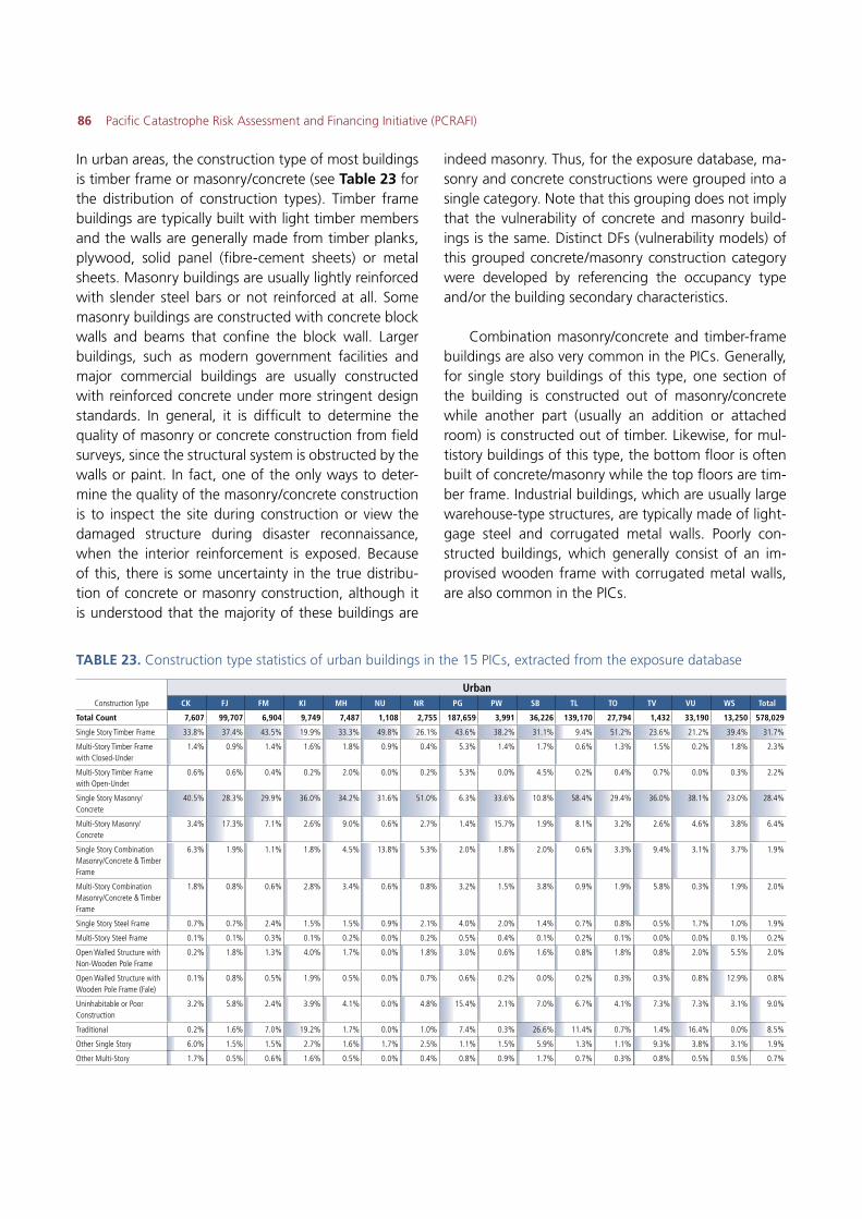
86 Pacific Catastrophe Risk Assessment and Financing Initiative (PCRAFI)
In urban areas, the construction type of most buildings is timber frame or masonry/concrete (see Table 23 for the distribution of construction types). Timber frame buildings are typically built with light timber members and the walls are generally made from timber planks, plywood, solid panel (fibre-cement sheets) or metal sheets. Masonry buildings are usually lightly reinforced with slender steel bars or not reinforced at all. Some masonry buildings are constructed with concrete block walls and beams that confine the block wall. Larger buildings, such as modern government facilities and major commercial buildings are usually constructed with reinforced concrete under more stringent design standards. In general, it is difficult to determine the quality of masonry or concrete construction from field surveys, since the structural system is obstructed by the walls or paint. In fact, one of the only ways to deter-mine the quality of the masonry/concrete construction is to inspect the site during construction or view the damaged structure during disaster reconnaissance, when the interior reinforcement is exposed. Because of this, there is some uncertainty in the true distribu-tion of concrete or masonry construction, although it is understood that the majority of these buildings are
indeed masonry. Thus, for the exposure database, ma-sonry and concrete constructions were grouped into a single category. Note that this grouping does not imply that the vulnerability of concrete and masonry build-ings is the same. Distinct DFs (vulnerability models) of this grouped concrete/masonry construction category were developed by referencing the occupancy type and/or the building secondary characteristics.
Combination masonry/concrete and timber-frame buildings are also very common in the PICs. Generally, for single story buildings of this type, one section of the building is constructed out of masonry/concrete while another part (usually an addition or attached room) is constructed out of timber. Likewise, for mul-tistory buildings of this type, the bottom floor is often built of concrete/masonry while the top floors are tim-ber frame. Industrial buildings, which are usually large warehouse-type structures, are typically made of light-gage steel and corrugated metal walls. Poorly con-structed buildings, which generally consist of an im-provised wooden frame with corrugated metal walls, are also common in the PICs.
TABLE 23. Construction type statistics of urban buildings in the 15 PICs, extracted from the exposure database
Construction Type
UrbanCK FJ FM KI MH NU NR PG PW SB TL TO TV VU WS Total
Total Count 7,607 99,707 6,904 9,749 7,487 1,108 2,755 187,659 3,991 36,226 139,170 27,794 1,432 33,190 13,250 578,029
Single Story Timber Frame 33.8% 37.4% 43.5% 19.9% 33.3% 49.8% 26.1% 43.6% 38.2% 31.1% 9.4% 51.2% 23.6% 21.2% 39.4% 31.7%
Multi-Story Timber Frame with Closed-Under
1.4% 0.9% 1.4% 1.6% 1.8% 0.9% 0.4% 5.3% 1.4% 1.7% 0.6% 1.3% 1.5% 0.2% 1.8% 2.3%
Multi-Story Timber Frame with Open-Under
0.6% 0.6% 0.4% 0.2% 2.0% 0.0% 0.2% 5.3% 0.0% 4.5% 0.2% 0.4% 0.7% 0.0% 0.3% 2.2%
Single Story Masonry/Concrete
40.5% 28.3% 29.9% 36.0% 34.2% 31.6% 51.0% 6.3% 33.6% 10.8% 58.4% 29.4% 36.0% 38.1% 23.0% 28.4%
Multi-Story Masonry/Concrete
3.4% 17.3% 7.1% 2.6% 9.0% 0.6% 2.7% 1.4% 15.7% 1.9% 8.1% 3.2% 2.6% 4.6% 3.8% 6.4%
Single Story Combination Masonry/Concrete & Timber Frame
6.3% 1.9% 1.1% 1.8% 4.5% 13.8% 5.3% 2.0% 1.8% 2.0% 0.6% 3.3% 9.4% 3.1% 3.7% 1.9%
Multi-Story Combination Masonry/Concrete & Timber Frame
1.8% 0.8% 0.6% 2.8% 3.4% 0.6% 0.8% 3.2% 1.5% 3.8% 0.9% 1.9% 5.8% 0.3% 1.9% 2.0%
Single Story Steel Frame 0.7% 0.7% 2.4% 1.5% 1.5% 0.9% 2.1% 4.0% 2.0% 1.4% 0.7% 0.8% 0.5% 1.7% 1.0% 1.9%
Multi-Story Steel Frame 0.1% 0.1% 0.3% 0.1% 0.2% 0.0% 0.2% 0.5% 0.4% 0.1% 0.2% 0.1% 0.0% 0.0% 0.1% 0.2%
Open Walled Structure with Non-Wooden Pole Frame
0.2% 1.8% 1.3% 4.0% 1.7% 0.0% 1.8% 3.0% 0.6% 1.6% 0.8% 1.8% 0.8% 2.0% 5.5% 2.0%
Open Walled Structure with Wooden Pole Frame (Fale)
0.1% 0.8% 0.5% 1.9% 0.5% 0.0% 0.7% 0.6% 0.2% 0.0% 0.2% 0.3% 0.3% 0.8% 12.9% 0.8%
Uninhabitable or Poor Construction
3.2% 5.8% 2.4% 3.9% 4.1% 0.0% 4.8% 15.4% 2.1% 7.0% 6.7% 4.1% 7.3% 7.3% 3.1% 9.0%
Traditional 0.2% 1.6% 7.0% 19.2% 1.7% 0.0% 1.0% 7.4% 0.3% 26.6% 11.4% 0.7% 1.4% 16.4% 0.0% 8.5%
Other Single Story 6.0% 1.5% 1.5% 2.7% 1.6% 1.7% 2.5% 1.1% 1.5% 5.9% 1.3% 1.1% 9.3% 3.8% 3.1% 1.9%
Other Multi-Story 1.7% 0.5% 0.6% 1.6% 0.5% 0.0% 0.4% 0.8% 0.9% 1.7% 0.7% 0.3% 0.8% 0.5% 0.5% 0.7%
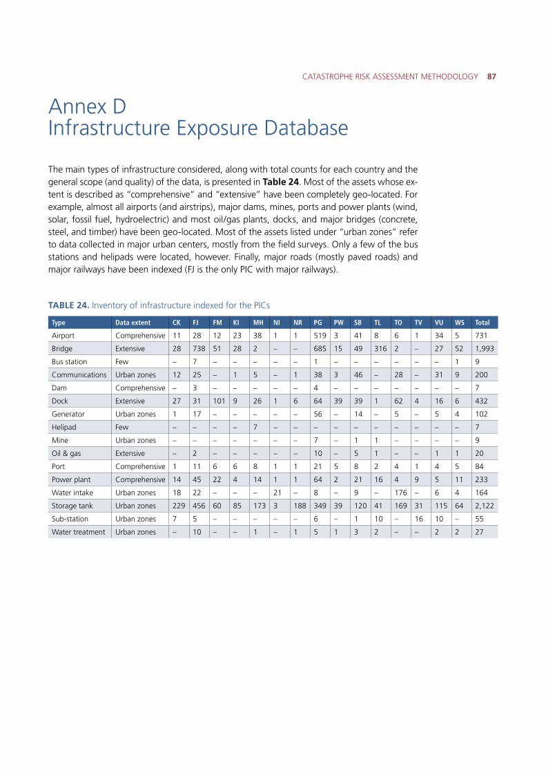
CATASTROPHE RISK ASSESSMENT METHODOLOGY 87
Annex D Infrastructure Exposure Database
The main types of infrastructure considered, along with total counts for each country and the general scope (and quality) of the data, is presented in Table 24. Most of the assets whose ex-tent is described as “comprehensive” and “extensive” have been completely geo-located. For example, almost all airports (and airstrips), major dams, mines, ports and power plants (wind, solar, fossil fuel, hydroelectric) and most oil/gas plants, docks, and major bridges (concrete, steel, and timber) have been geo-located. Most of the assets listed under “urban zones” refer to data collected in major urban centers, mostly from the field surveys. Only a few of the bus stations and helipads were located, however. Finally, major roads (mostly paved roads) and major railways have been indexed (FJ is the only PIC with major railways).
TABLE 24. Inventory of infrastructure indexed for the PICs
Type Data extent CK FJ FM KI MH NI NR PG PW SB TL TO TV VU WS Total
Airport Comprehensive 11 28 12 23 38 1 1 519 3 41 8 6 1 34 5 731
Bridge Extensive 28 738 51 28 2 – – 685 15 49 316 2 – 27 52 1,993
Bus station Few – 7 – – – – – 1 – – – – – – 1 9
Communications Urban zones 12 25 – 1 5 – 1 38 3 46 – 28 – 31 9 200
Dam Comprehensive – 3 – – – – – 4 – – – – – – – 7
Dock Extensive 27 31 101 9 26 1 6 64 39 39 1 62 4 16 6 432
Generator Urban zones 1 17 – – – – – 56 – 14 – 5 – 5 4 102
Helipad Few – – – – 7 – – – – – – – – – – 7
Mine Urban zones – – – – – – – 7 – 1 1 – – – – 9
Oil & gas Extensive – 2 – – – – – 10 – 5 1 – – 1 1 20
Port Comprehensive 1 11 6 6 8 1 1 21 5 8 2 4 1 4 5 84
Power plant Comprehensive 14 45 22 4 14 1 1 64 2 21 16 4 9 5 11 233
Water intake Urban zones 18 22 – – – 21 – 8 – 9 – 176 – 6 4 164
Storage tank Urban zones 229 456 60 85 173 3 188 349 39 120 41 169 31 115 64 2,122
Sub-station Urban zones 7 5 – – – – – 6 – 1 10 – 16 10 – 55
Water treatment Urban zones – 10 – – 1 – 1 5 1 3 2 – – 2 2 27
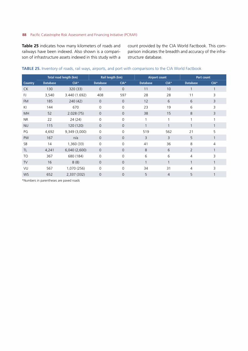
88 Pacific Catastrophe Risk Assessment and Financing Initiative (PCRAFI)
TABLE 25. Inventory of roads, rail ways, airports, and port with comparisons to the CIA World Factbook
Country
Total road length (km) Rail length (km) Airport count Port count
Database CIA* Database CIA* Database CIA* Database CIA*
CK 130 320 (33) 0 0 11 10 1 1
FJ 3,540 3.440 (1.692) 408 597 28 28 11 3
FM 185 240 (42) 0 0 12 6 6 3
KI 144 670 0 0 23 19 6 3
MH 52 2.028 (75) 0 0 38 15 8 3
NR 22 24 (24) 0 0 1 1 1 1
NU 115 120 (120) 0 0 1 1 1 1
PG 4,692 9,349 (3,000) 0 0 519 562 21 5
PW 167 n/a 0 0 3 3 5 1
SB 14 1,360 (33) 0 0 41 36 8 4
TL 4,241 6,040 (2,600) 0 0 8 6 2 1
TO 367 680 (184) 0 0 6 6 4 3
TV 16 8 (8) 0 0 1 1 1 1
VU 567 1,070 (256) 0 0 34 31 4 3
WS 652 2,337 (332) 0 0 5 4 5 1
*Numbers in parentheses are paved roads
Table 25 indicates how many kilometers of roads and railways have been indexed. Also shown is a compari-son of infrastructure assets indexed in this study with a
count provided by the CIA World Factbook. This com-parison indicates the breadth and accuracy of the infra-structure database.
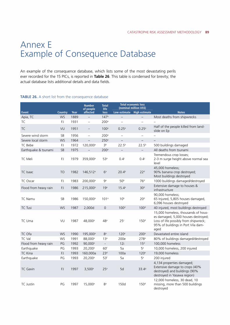
CATASTROPHE RISK ASSESSMENT METHODOLOGY 89
Annex E Example of Consequence Database
An example of the consequence database, which lists some of the most devastating perils ever recorded for the 15 PICs, is reported in Table 26. This table is condensed for brevity; the actual database lists additional details and data fields.
TABLE 26. A short list from the consequence database
Event Country Year
Number of people affected
Total life loss
Total economic loss(nominal million US$)
NotesLow estimate High estimate
Apia, TC WS 1889 – 147b – – Most deaths from shipwrecks TC FJ 1931 – 200a – – –
TC VU 1951 – 100a 0.25a 0.25a Half of the people killed from land-slide on Ep
Severe wind storm SB 1956 – 200a – – –Severe local storm WS 1964 – 250a – – –TC Bebe FJ 1972 120,000a 3b 22.5b 22.5b 500 buildings damaged Earthquake & tsunami SB 1975 – 200a – – All deaths from tsunami
TC Meli FJ 1979 359,000a 53a 0.4c 0.4c
Tremendous crop losses; 2-3 m surge height above normal sea level
TC Isaac TO 1982 146,512a 6a 20.4b 22d
45,000 homeless;90% banana crop destroyed;Most buildings destroyed
TC Oscar FJ 1983 200,000a 9a 50b 76d 1000 buildings damaged/destroyed
Flood from heavy rain FJ 1986 215,000a 19a 15.4a 30d Extensive damage to houses & infrastructure
TC Namu SB 1986 150,000a 101a 10b 20d
90,000 homeless;65 Injured, 5,805 houses damaged, 6,096 houses destroyed
TC Tusi WS 1987 2,000d 0 100d 100d 40 injured, most buildings destroyed
TC Uma VU 1987 48,000a 48a 25c 150d
15,000 homeless, thousands of hous-es damaged, 5,000 houses destroyed;Loss of life possibly from shipwreck;95% of buildings in Port Vila dam-aged
TC Ofa WS 1990 195,000a 8a 120e 200a Devastated entire island TC Val WS 1991 88,000a 13a 200e 278a 80% of buildings damaged/destroyed Flood from heavy rain PG 1992 90,000a - 12i 15d 100,000 homeless Earthquake PG 1993 20,200a 60f 5a 5a 10,000 homeless, 200 injured TC Kina FJ 1993 160,000a 23d 100a 120e 19,000 homeless Earthquake PG 1993 20,200a 53f 5a 5a 200 injured
TC Gavin FJ 1997 3,500a 25a 5d 33.4g
4,134 properties damaged;Extensive damage to crops (40% destroyed) and buildings (90% destroyed in Yasawa region)
TC Justin PG 1997 15,000a 8a 150d 150d
12,000 homeless, 30 dead, 10 missing, more than 500 buildings destroyed
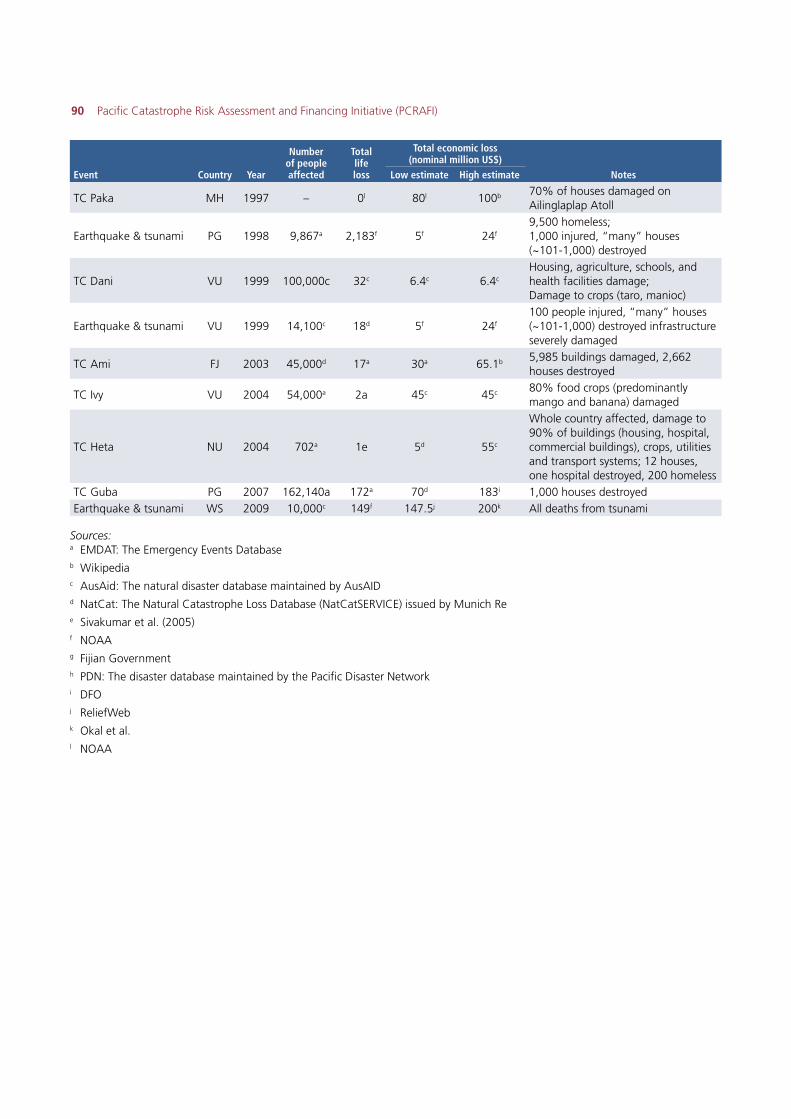
90 Pacific Catastrophe Risk Assessment and Financing Initiative (PCRAFI)
Event Country Year
Number of people affected
Total life loss
Total economic loss(nominal million US$)
NotesLow estimate High estimate
TC Paka MH 1997 – 0l 80l 100b 70% of houses damaged on Ailinglaplap Atoll
Earthquake & tsunami PG 1998 9,867a 2,183f 5f 24f
9,500 homeless;1,000 injured, “many” houses (~101-1,000) destroyed
TC Dani VU 1999 100,000c 32c 6.4c 6.4c
Housing, agriculture, schools, and health facilities damage;Damage to crops (taro, manioc)
Earthquake & tsunami VU 1999 14,100c 18d 5f 24f
100 people injured, “many” houses (~101-1,000) destroyed infrastructure severely damaged
TC Ami FJ 2003 45,000d 17a 30a 65.1b 5,985 buildings damaged, 2,662 houses destroyed
TC Ivy VU 2004 54,000a 2a 45c 45c 80% food crops (predominantly mango and banana) damaged
TC Heta NU 2004 702a 1e 5d 55c
Whole country affected, damage to 90% of buildings (housing, hospital, commercial buildings), crops, utilities and transport systems; 12 houses, one hospital destroyed, 200 homeless
TC Guba PG 2007 162,140a 172a 70d 183i 1,000 houses destroyed Earthquake & tsunami WS 2009 10,000c 149f 147.5j 200k All deaths from tsunami
Sources:a EMDAT: The Emergency Events Database b Wikipedia c AusAid: The natural disaster database maintained by AusAID d NatCat: The Natural Catastrophe Loss Database (NatCatSERVICE) issued by Munich Re e Sivakumar et al. (2005) f NOAAg Fijian Government h PDN: The disaster database maintained by the Pacific Disaster Network i DFO j ReliefWeb k Okal et al. l NOAA
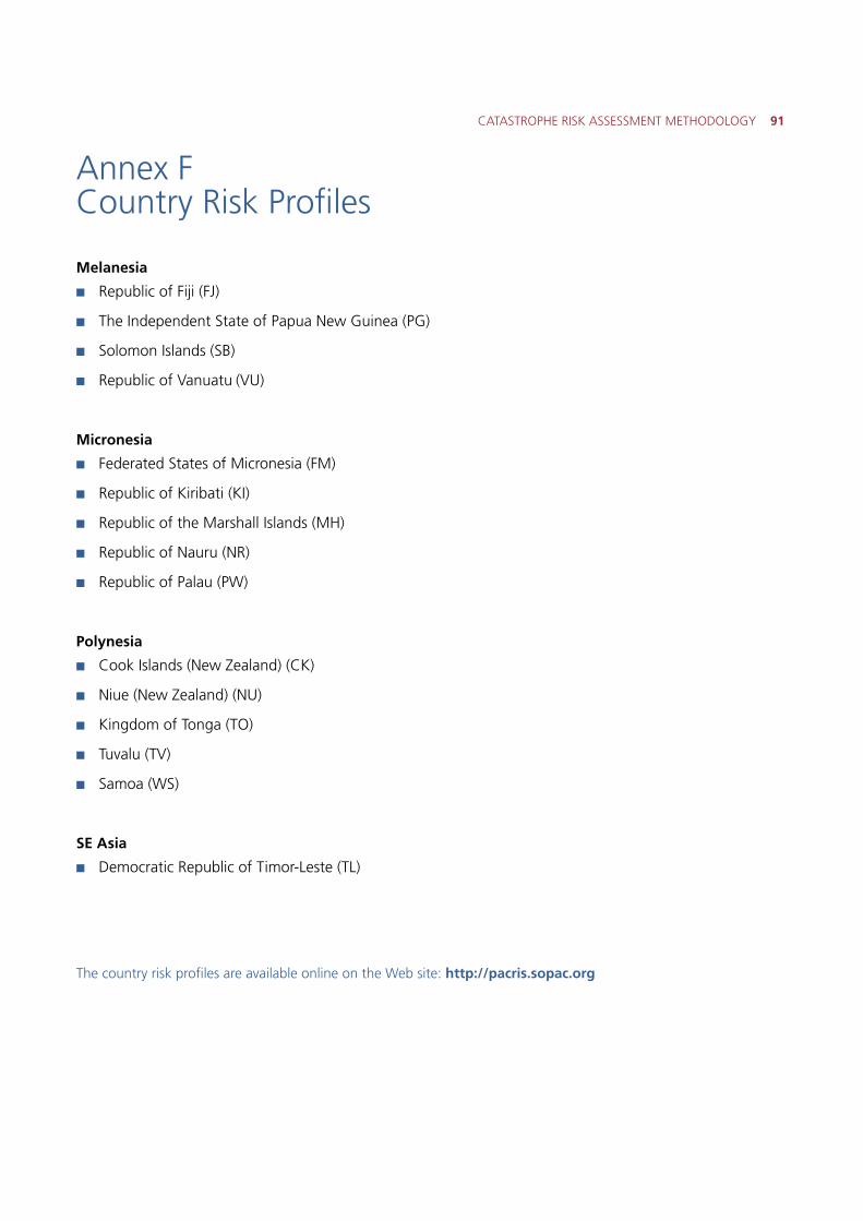
CATASTROPHE RISK ASSESSMENT METHODOLOGY 91
Annex F Country Risk Profiles
Melanesia
�� Republic of Fiji (FJ)
�� The Independent State of Papua New Guinea (PG)
�� Solomon Islands (SB)
�� Republic of Vanuatu (VU)
Micronesia
�� Federated States of Micronesia (FM)
�� Republic of Kiribati (KI)
�� Republic of the Marshall Islands (MH)
�� Republic of Nauru (NR)
�� Republic of Palau (PW)
Polynesia
�� Cook Islands (New Zealand) (CK)
�� Niue (New Zealand) (NU)
�� Kingdom of Tonga (TO)
�� Tuvalu (TV)
�� Samoa (WS)
SE Asia
�� Democratic Republic of Timor-Leste (TL)
The country risk profiles are available online on the Web site: http://pacris.sopac.org

The World Bank1818 H Street, N.W. Washington D.C. 20433, USA