Impact of Supply Chain Strategies on Bullwhip Effect

Sevtap Çatalbaş

Submitted to the

Institute of Graduate Studies and Research

in partial fulfillment of the requirements for the Degree of

Master of Science in

Industrial Engineering

Eastern Mediterranean University

March 2009, Gazimagusa

North Cyprus

Approval of the Institute of Graduate Studies and Research

___________________________ Prof. Dr. Elvan Yılmaz Director (a)

I certify that this thesis satisfies the requirements as a thesis for the degree of Master of Science in Industrial Engineering.

____________________________ Asst. Prof. Dr. Gökhan Đzbırak Chair, Department of Industrial Engineering

We certify that we have read this thesis and that in our opinion it is fully adequate in scope and quality as a thesis for the degree of Master of Science in Industrial Engineering.

____________________________ Assoc. Prof. Dr. Nureddin Kırkavak Supervisor

Examining Committee

1. Assoc. Prof. Dr. Bela Vizvari ________________________

2. Assoc. Prof. Dr. Nureddin Kırkavak _________________________

3. Asst. Prof. Dr. Adham Mackieh _________________________

iii

ABSTRACT

IMPACT OF SUPPLY CHAIN STRATEGIES

ON BULLWHIP EFFECT

Changes of today’s firm’s competitiveness strategies from firms level to improved

Supply Chain level causes increases in number and importance of Supply Chain studies

in the literature. Variation between demand and orders is became the most important

problem and most studied Supply Chain topic. This problem named in literature as

Bullwhip Effect, is studied in this thesis with possible 11 factors effect on bullwhip. By

using the improved Bullwhip Effect formula; lead time, review period, demand

distribution, ordering cost, numbers of forecast periods are found as the factors which

have significant effect on Bullwhip. In addition to this, for the use of similar Supply

Chain researches, or real Supply Chain members, an improved spreadsheet simulation

tool is prepared to test the proposed Supply Chain structures effects on different Supply

Chain performance measures.

Keyword: Supply Chain, Bullwhip Effect, Spreadsheets, Simulation.

iv

ÖZET

FARKLI TEDARĐK ZĐNCĐRĐ STRATEJĐLERĐNĐN

KAMÇI ETKĐSĐ ÜZERĐNDEKĐ SONUÇLARI

Günümüzde işletmelerin birbirleriyle olan rekabetinin, firmalar arası düzeyden güçlü ve

gelişmiş tedarik zinciri düzeyine çıkarması, literatürdeki Tedarik Zinciri çalışmalarının

önem kazanmasına ve artmasına sebep olmuştur. Talep ve siparişteki belirsizlik ve

dalgalanmaların, tedarik ziniciri üzerindeki etkisi en büyük sorun ve en çok üzerinde

çalışma yapılan konulardan biri olmuştur. Kamçı etkisi, olarak adlandırılan bu sorun ve

bu etkiyi tetiklediği düşünülen 11 faktör, bu çalışmada incelenmiştir. Kamçı etkisi

formülünün de geliştirilmesi sağlanarak, bekleme süresi, sipariş çevrim süresi, talep

dağılımı, sipariş verme maliyeti, talep tahmin süresi gibi faktörlerin Kamçı etkisi

üzerinde belirgin sonuçları olduğu tespit edilmiştir. Buna ek olarak, farklı tedarik zinciri

yapılarının, performans ölçümlerine olan etkisinin incelenmesini sağlayan, elektronik

tablolar yardımıyla hazırlanmış yeni bir simulasyon aracı, akademik veya endüstriyel

çalışmaların kullanımına sunulmuştur.

Anahtar Kelimeler: Tedarik Zinciri, Kamçı Etkisi, Elektronik Tablolar, Benzetim.

v

TABLE OF CONTENTS

ABSTRACT.………………………………………….…………...……………………iii

ÖZET ............................................................................................................................... iv

LIST OF TABLES.......................................................................................................... vi

LIST OF FIGURES....................................................................................................... vii

CHAPTER 1: INTRODUCTION .................................................................................. 1

CHAPTER 2: LITERATURE REVIEW ...................................................................... 5

CHAPTER 3: METHODOLOGY ............................................................................... 17

CHAPTER 4: DESIGN OF EXPERIMENT .............................................................. 23

4.1 Input Module ......................................................................................................... 24

4.2 Calculation Module ............................................................................................... 30

4.3 Output Module……………………………………………………………….…...35

CHAPTER 5: EXPERIMENTAL ANALYSIS .......................................................... 39

5.1 Analysis for standard out policy…….…………………………………………....42

5.2 Analysis for lot for lot policy: ............................................................................... 47

CHAPTER 6: CONCLUSION ..................................................................................... 52

REFERENCES .............................................................................................................. 56

APPENDIX .................................................................................................................... 61

vi

LIST OF TABLES

Table 5.1: Factors for standard out policy and lot for lot policy ………………………41

Table 5.1.1: Analysis of Variance for BULLWHIP with Standard out policy…...……44

Table 5.2.1: Analysis of Variance for BULLWHIP with Lot for lot policy….…..……49

vii

LIST OF FIGURES

Figure 4.1: Supply Chain Structure…….………………………………………….……23

Figure 4.1.1: Spreadsheet simulation input module…………………………….…………24

Figure.4.2.1: Spreadsheet Simulation Calculation Module…………………….….………30

Figure 4.2.2: Bullwhip Effect Graph………………...……………………….……….….31

Figure 5.1.1: Normal Probability Plot for standard out policy....…………….…………42

Figure 5.1.2: Residual plot for standard out policy………………………….……….…43

Figure 5.1.3: Main effects plot for standard out policy……………………….…...……45

Figure 5.1.4: Pareto chart for standard out policy………………………...….…………46

Figure 5.2.1: Normal Probability Plot for lot for lot policy………………….…………47

Figure 5.2.2: Residuals Plot for lot for lot policy…………………………….…………48

Figure 5.2.3: Main effects Plot for lot for lot policy………………………...….………50

Figure 5.2.4: Pareto Chart for lot for lot policy………………………………….…...…51

viii

Figure A. 1: Input analyzer results of random demand generation for normal distribution

with mean 10 and variance 1……………………………………………………………62

Figure A.2: Input analyzer results of random demand generation for normal distribution

with mean 10 and variance 5……………………………………………………………63

Figure A.3: Input analyzer results of random demand generation for normal distribution

with mean 25 and variance 1……………………………………………………………64

Figure A.4: Input analyzer results of random demand generation for normal distribution

with mean 25 and variance 5……………………………………………………………65

Figure A.5: Input analyzer results of random demand generation for uniform distribution

with a=8 and b=12 (mean 10 variance 1)………………………………………….……66

Figure A.6: Input analyzer results of random demand generation for uniform distribution

with a=1 and b=19 (mean 10 variance 5)……………………………………….………67

Figure A.7: Input analyzer results of random demand generation for uniform distribution

with a=23 and b=27 (mean 25 variance 1)…………………………………...…………68

Figure A.8: Input analyzer results of random demand generation for uniform

distribution with a=16 and b=34 (mean 25 variance 5)…………………………….…...69

ix

Figure A.9: A Sample Simulation spreadsheet for standard out policy…………...……70

Figure A.10: ANOVA results for Bullwhip with Standard out Policy……...……….…71

Figure A.11: Estimated Effects and Coefficients for Bullwhip with Standard out

Policy……………………………………………………………………………………73

Figure A.12: Least Square Means for Bullwhip with Standard out Policy…..................75

Figure A.13: A Sample Simulation spreadsheet for lot for lot policy…..........................83

Figure A.14: ANOVA results for Bullwhip with Lot for Lot Policy…………………...84

Figure A.15: Estimated Effects and Coefficients for Bullwhip with Lot for Lot

Policy…………………………………………………………………………………....87

Figure A.16: Least Square Means for Bullwhip with Lot for Lot Policy …................…89

Figure A.17: Factors interaction plot for standard out policy……………………..........97

Figure A.18: Factors full interaction plot for standard out policy…………………........97

x

Figure A.19: Factors interaction plot for lot for lot policy…………………………...…98

Figure A.20: Factors full interaction plot for lot for lot policy ….................………….98

1

CHAPTER 1

INTRODUCTION

In today’s global marketplace, competition between firms is not limited to brand names

and products; the success of a firm depends on the true management of the Supply Chain

members.

Companies work with several suppliers, starting from the ordering of raw material until

converting this raw material into finished products and delivery of the products to

customers. The coordination and management of information, material and money flow

within a company and its suppliers is hard and complex process. Several problems occur

related to delivery time, quality and quantity of products.

The problems between suppliers and company directly affect the final product’s quality

and the company’s image. ‘Supply Chain Management’ is a term which aims to prevent

possible Supply Chain problems and find solutions and make improvements for this

chain.

Supply Chain Management defined as an integrated management of suppliers,

companies and customers to provide in shortest time, products with highest quality and

lowest cost.

2

The scope of the Supply Chain is very wide; it includes different research topics

according to the problem. For example; for the decisions of suppliers selection,

‘Supplier Selection Methods’, location of suppliers, ‘Supply Chain Network’ are the

new topics in the literature which is defined according to the increasing attention and

importance of Supply Chain problems. Number of suppliers in the chain, information

sharing strategies, and cost policies can also be other examples for Supply Chain

research topics.

The most important and significant problem in the chain is related with the demand and

orders. Because in any Supply Chain, even one stage Supply Chain there is a variation

difference between orders and demand. It is proven in the literature that variation of

orders increases as one move up in the chain and this is defined as ‘Bullwhip Effect’.

This variation difference causes increasing ordering and inventory holding cost. In

addition to this delivery time and order quantity problems causes a decrease in customer

satisfaction with increase in backorder costs.

Several studies made for the causes and results of Bullwhip Effect. Some researchers

tried to investigate factors causing Bullwhip Effect some of them tried to find solutions

to reduce the adverse effect of bullwhip by using different methods; simulation and/or

case studies.

This thesis aim is to determine the Impact of Supply Chain Strategies on Bullwhip

Effect. In literature there are different researches related to Bullwhip Effect which

increases day by day. But most of the studies are case studies and there can be a solution

3

guideline only for similar cases defined in the research and not sufficient to make

general result for the Bullwhip Effect.

In this study, firstly a new, improved simulation tool will be built. By this simulation

tool any Supply Chain strategies will be tested, and tool can be downloaded and used by

any Supply Chain member. Since it is modeled with Ms Excel, this is a user friendly

simulation tool and not complex and costly as other simulation tools.

Second step is the determination of possible factors that can cause Bullwhip Effect. In

literature there are similar studies deals with factors effect on bullwhip. But those studies

limited with only three or four factors combination. In this thesis study, 11 factors,

which are, demand forecasting technique, demand distribution type, ordering cost,

holding cost, backorder cost, and demand mean, demand variance, number of forecast

periods, lead time, review periods and service level. Effects on bullwhip will be detected

according to two different ordering policies; lot for lot and standard out policies.

Review period is one of the most important factors but in literature generally it is

assumed as 1 and not studied its effect on bullwhip. The reason for this is the defined

Bullwhip Effect formula in the literature; it causes misleading results in different review

periods. In this thesis Bullwhip Effect formula also improved to solve this problem.

Bullwhip Effect is the most important and common performance measure. But

additionally to this, net stock amplification, holding, backorder, ordering and total cost

are the other performance measures added to simulation tool to be able to simulate more

real cases and have more accurate results.

4

Finally two different design analysis will be made to have valid and accurate results and

comments for the impacts of different Supply Chain strategies on Bullwhip Effect for

two different ordering polices.

As a conclusion, this thesis will provide a new simulation tool for Bullwhip Effect

studies with an improved Bullwhip Effect formula. Design analysis will be made for all

factors defined in literature and faced in real life to show their effects on bullwhip and

make suggestion to reduce Bullwhip Effect in any Supply Chain.

The thesis will continue with a complete Supply Chain literature review, following with

a Methodology chapter to explain simulation in detail, then in Design of Experiment

Chapter simulation results will be analyzed, and design results and suggestion for the

solution of Bullwhip Effect problem will be given in conclusion Chapter.

5

CHAPTER 2

LITERATURE REVIEW

Supply Chain Management is defined in the literature, as an integrated management

policy of suppliers, companies and customers, to provide the right raw material, the right

product, the right delivery method with the lowest cost and highest quality.

Beamon B.M. (1998) states that “A Supply Chain may be defined as an integrated

process wherein suppliers, manufacturers, distributors, and retailers work together in an

effort to: obtain raw materials, convert these raw materials into specified final products,

and deliver these final products to retailers. This chain is traditionally characterized by a

forward flow of materials and a backward flow of information”.

Min and Zhou (2002) suggests two main business process in a Supply Chain to provide

that material and information flow. The business processes are defined as material

management and physical distribution. Material management refers to the inbound

logistics such as production control, warehousing, shipping and transportation of

finished products.

Physical distribution refers to outbound logistics that are pricing, promotional support,

returned product handling and life cycle support. For a Supply Chain this combination of

6

material management and physical distribution activities causes multiple business

networks and relations instead of linear one to one business relationships.

The limits and contents of each Supply Chain’s nonlinear relation network are not same

for every Manufacturing or Service Company. For this reason, before modeling a Supply

Chain, the first step that a model builder should do is defining the scope of Supply Chain

model. As Min and Zhou (2002) states there is no systematic way of defining the scope

of Supply Chain problem. But there are different guidelines in the literature. One of

them is proposed by Stevens (1989). This guideline is consisting of three levels of

decision hierarchy. First one is competitive strategy which includes location-allocation

decisions, demand planning, distribution channel planning, strategic alliances, new

product development, outsourcing, supplier selection, information technology selection,

pricing, and network restructuring. Secondly tactical plans; includes inventory control,

production/distribution coordination, order/freight consolidation, material handling,

equipment selection, and layout design. Finally operational routines; that includes

vehicle routing/scheduling, workforce scheduling, record keeping, and packaging

Another guideline to follow is suggested by Cooper et al. (1997b). The three structures

of a Supply Chain network suggested is: (1) the type of a Supply Chain partnership

which can be primary and secondary; (2) the structural dimensions of a Supply Chain

network that can be horizontal and vertical; (3) the characteristics of process links

among Supply Chain partners such as managed business process links (firm integrates a

Supply Chain process with one or more customers/suppliers), monitored business

process links (firm is involved in monitoring or auditing how the link is integrated and

7

managed), not managed business process links (firm fully trusts its partners' ability to

manage the process links and leaves the management responsibility up to them), and

non-member business links (that are the ones between both partners and non-members

of the company's Supply Chain).

Defining the scope of the Supply Chain model helps to construct the structure of the

model. But to adopt the model more close to real life situations the decision variables,

constraints and suitable performance measures should be added to the model according

to defined Supply Chain structure.

Since the Supply Chain structure is not same for every company, the decision variables

and constraints are not same too. But there are some common examples in the literature

that can be applied to most of the Supply Chain Models.

Decision variables can be; location, allocation, network structuring, number of facilities

and equipment, service sequence, volume, size of workforce, extent of outsourcing,

production/distribution scheduling, number of echelons, plant product assignment, buyer

supplier relationships and number of product types held in inventory.

Constraints of the Supply Chain model can include capacity, service compliance (e.g.

delivery time windows manufacturing due dates, maximum holding time for backorders,

number of driving hours for truck drivers), and extend of demand.

8

Beamon B.M. (1998) states that “Supply Chain performance measures are categorized as

either qualitative or quantitative. For qualitative performance measures: there is no

single direct numerical measurement and quantitative performance measures: may be

directly described numerically”. The qualitative performance measures defined as

Customer Satisfaction, Flexibility, Information and Material Flow Integration, Effective

Risk Management and Supplier Performance. The quantitative performance measures

are also divided into two categories according to measures based on cost and measures

based on customer responsiveness. For first category Cost Minimization, Sales

Maximization, Profit Maximization, Inventory Investment Minimization and Return on

Investment Maximization are given. For the second category that the measures based on

customer responsiveness, the performance measures can be Fill Rate Maximization,

Product Lateness Minimization, Customer Response Time Minimization, Lead Time

Minimization and Function Duplication Minimization.

In this section, scope of the Supply Chain is defined; the required decision variables,

performance measures and constraints are also explained for any Supply Chain structure.

Researchers are used, defined constraints, decision variables and performance measure

as a guideline for their study. The important part is to modify and adopt the given

information of literature to the studied Supply Chain model.

Supply Chains are modeled especially to investigate and solve possible problems in the

chain. As a result of experiments made related to Supply Chain, researchers discovered a

common problem for all Supply Chains. This common problem is the increase of

demand order variability as one move up the Supply Chain. All studies concludes that

9

the variation of demand and orders have important effects to Supply Chain performance

measures. This problem named in the literature as “Bullwhip Effect”.

The first researcher of Bullwhip Effect was Forrester (1958). He did not use term as

“bullwhip” but he defined as “Demand Amplification” and shows that there is variation

between customers demand and manufacturer orders. His valuable study encourages

other researchers to make studies related to “Bullwhip Effect” to make improvements

for Supply Chain by determining causes and solutions of this problem.

Bullwhip Effect is studied by several researchers. Some of them tried to show that

bullwhip existence in every Supply Chain, and some of them tried to find possible

causes and solutions of Bullwhip Effect.

Lee et all. (1997) shows that there are five main causes of the Bullwhip Effect: The uses

of demand forecasting, supply shortages, lead times, batch ordering, and price

variations.

There are different models and methods to show Bullwhip Effect. The most popular one

is the “Beer Distribution Game”. In this game, 4-stage Supply Chain, which consisting

of a factory, a distributor, a wholesaler and a retailer is modeled. This game aim is to

provide a simulation area for players, to show causes of Bullwhip Effect and see the

results of proposed solutions to Supply Chain performance. Simchi-Levi et al. (2000)

[24]. improved beer game in to a computerized version. Today, researchers can use any

10

version of beer game such as manual or computerized also web-based versions (e.g.

Machuca and Barajas 1997, Chen 1998).

Beer game is not only used as a Supply Chain simulation tool. It also helps researches to

understand the concept of Supply Chain. Some of the researchers not used that beer

game simulation. They generate their own simulation tool or use any other tools. But as

a common point the other Supply Chain simulation tools or methods are based on beer

game’s Supply Chain model with modified or improved versions.

Every Supply Chain has different Bullwhip Effect causes and different solutions. But

when literate reviewed, it can be seen that there are some common problems and

common solutions for Bullwhip Effect. Only need in literature is a single study, which

examines all proposed bullwhip causes with all suggested solution techniques.

Chen et al. (1998) quantify the Bullwhip Effect in a simple 2-stage Supply Chain, to

determine the effect of forecasting, lead times and information. They conclude that with

moving average forecasting technique longer lead times are increases Bullwhip Effect.

And centralized customer information that means, all Supply Chain members can have

same access to customer demand information, by this way Bullwhip Effect can not be

eliminated but can be reduced.

Manyem et al. (1999) is another example of a Bullwhip Effect simulation with similar

results. They discussed the factors that influence Bullwhip Effect and its impact on

profitability by using Supply Chain simulation. Conclusions are same, centralized

11

information sharing strategy, has positive effect on bullwhip and also shorter lead time

gives better Bullwhip Effects measures.

Cantor (2008) made a laboratory beer game simulation. In this study students come to

laboratory and plays beer game by this way researcher have a dynamic simulation

environment to see the effect of demand model and lead time on bullwhip.

Literature of Bullwhip Effect is mainly consisting of studies deals with investigation of

Bullwhip Effect causes or quantifying the determined factors effects on bullwhip. Lead

time, information sharing strategies and ordering policies are the common factors of

Bullwhip Effect. Demand forecasting technique, ordering decisions, review period, and

cost structure are the other important factors that affect bullwhip. But there is no single

study which shows and discusses all bullwhip causes and their effects under different

Supply Chain strategies. And the other important point is that, researcher chooses one of

them, either generating their own Supply Chain simulation tool, or use predetermined

simulation tool and make experiment for their proposed solution by using that tool.

Supply Chain studies can be done with different methods. Most important part is the

modeling the Supply Chain. Some examples for Supply Chain modeling for Bullwhip

Effect are given. Most of them are used simulation method. But in addition to this, there

are some other Supply Chain modeling approaches, which will be explained with details

in the following section.

Beamon B.M. (1998) states that mainly there are four Supply Chain Modeling

approaches which are; Deterministic Analytical Models, Stochastic Analytical Models,

12

Economic Models and Simulation models. Beamon B.M (1998) states that first three

models (Deterministic Analytical Models, Stochastic Analytical Models and Economic

Models) are used to find best algorithms or heuristics mainly for manufacturing

companies.

In general these models focus on some important parts of production as minimizing lead

time (the amount of time between the placing of an order and the receipt of the goods

ordered.), smoothing demand variances, and scheduling production. Simulation Models

are used for both manufacturing companies and for the service industry. This model aim

is to modeling real life situations in simulation module to identify the problems and find

ways to fix these problems.

Min and Zhou (2002) modified this classification and divide Supply Chain models into

four different classes. First one is deterministic (non-probabilistic); second one is

stochastic (probabilistic); third one is hybrid; and the last one is IT-driven models. As

seen here there are similarities between two classifications. But Min and Zhou (2002)

explains their classification as; “Deterministic models assume that all the model

parameters are known and fixed with certainty, whereas stochastic models take into

account the uncertain and random parameters.

The categories of decision analysis and queuing models from stochastic models are

excluded, because the literature indicates that Supply Chain models rarely used such

techniques. Hybrid models have elements of both deterministic and stochastic models.

These models include inventory-theoretic and simulation models that are capable of

13

dealing with both certainty and uncertainty involving model parameters. Considering the

proliferation of IT applications for Supply Chain modeling, we decided to add the

category of IT-driven models to the taxonomy.

IT-driven models aim to integrate and coordinate various phases of Supply Chain

planning on real-time basis using application software so that they can enhance visibility

throughout the Supply Chain”.

The difficult decision is to select the best modeling approach for a Supply Chain. But

choosing the right modeling approach is not enough; researchers also need to modify

this model according to defined performance measure, decision variables and constraints

of Supply Chain. To improve the knowledge of modeling approaches in Supply Chain,

the examples of past studies that researchers made using different modeling approaches

will be explained.

• Deterministic modeling approach; Ishii (1988) determined the base stock levels

and lead times associated with the lowest cost solution for an integrated Supply Chain

on a finite horizon. Cohen and Moon (1990) developed a constrained optimization

model, called PILOT, to investigate the effects of various parameters on Supply Chain

cost, and consider the additional problem of determining which manufacturing facilities

and distribution centers should be open. Nozick and Turnquist (2001) proposed an

approximate inventory cost function and then embedded it into a fixed-charge facility

location model. The fixed-charge facility location model was designed to consider a

14

tradeoff between demand coverage and cost associated with the location of automobile

distribution centers.

• Stochastic modeling approach; Cohen and Lee (1989) developed model for

establishing a material requirements policy for all materials for every stage in the Supply

Chain production system. They use four different cost-based sub-models which are;

Material Control, Production Control, Warehouse and Distribution. Pyke and Cohen

(1990), considered an integrated Supply Chain with one manufacturing facility, one

warehouse, and one retailer, and consider multiple product types. This model yields the

approximate economic reorder interval, replenishment batch sizes, and the order-up-to

product levels for a particular Supply Chain network. Swaminathan and Tayur (1999)

solved a so-called vanilla box problem where the inventories of semi-finished products

were stored in vanilla boxes and then were assembled into final products after a

customer actually ordered them further into the Supply Chain. Their model considered

random customer orders.

• Hybrid modeling approach; Karmarkar and Patel (1977) used a decomposition

approach to solve a single product, single period, multiple location inventory problems

with stochastic demands and transshipment between locations. To consider interactions

between inventory management and transportation modal choice. Cachon (1999) utilized

a game theory to take into account an infinite horizon, stochastic demand inventory

problem between one supplier and one retailer. In his game theory, Cachon (1999)

considered the possibility of ‘double marginalization’ (profit sharing between the

15

supplier and the retailer), buy-back contracts, and quantity discounts to develop the

optimal joint inventory policy. Karabakal et al. (2000) used a combination of simulation

and mixed-integer programming models to determine the number and location of

automobile distribution and processing centers as well as the set of market areas covered

by each distribution and processing center, while evaluating customer performance

measures such as the ability of Supply Chains to deliver a customer's preferred vehicle

within short time windows.

• IT-driven modeling approach; Camm et al. (1997) combined an integer

programming model involving the location of distribution centers and sourcing of

multiple products with a GIS to develop a flexible decision support system (DSS).

However, their model-based DSS did not include capacity constraints. Talluri (2000)

proposed a goal programming model for an effective acquisition and justification of IT

for a Supply Chain. The model could be useful in selecting the right ERP system that

can consider system acquisition and maintenance costs, flexibility, execution accuracy,

and compatibility.

• Simulation modeling approach: Towill (1992) [28] chooses simulation

techniques to evaluate the effects of various Supply Chain strategies on demand

amplification. The just-in-time strategy and the echelon Removal strategy are observed

to be the most effective in smoothing demand variations. Wikner, (1991) examines five

Supply Chain improvement strategies, and then implements these strategies on a three-

stage reference Supply Chain model.

16

Most effective improvement strategy is, improving the flow of information at all levels

throughout the chain, and separating orders

In this thesis study simulation modeling approach is chosen. The reasons to select this

method, its advantages and disadvantages will be explained in the following

“methodology” section.

17

CHAPTER 3

METHODOLOGY

Supply Chain can be modeled with stochastic, hybrid, information technology (it)-driven

or simulation modeling approaches. The type of modeling method should be chosen

according to the defined problem and Supply Chain structure.

In this study, impact of Supply Chain strategies on Bullwhip Effect is examined. In

addition to this, all different Supply Chain strategies effect on other performance

measures such as net stock amplification and the total cost are mentioned as another

discussion topic of this study.

The Supply Chain model should be capable enough to show the consequences of any

increase or decrease of factors to performance measures. For this reason, most suitable

modeling tool for this type of Supply Chain study is chosen as ‘simulation’. Details for

simulation method and sample Supply Chain simulation studies are given to better

explain the other reasons for selection of the simulation method.

Y. Chang et al. (2001) states that Supply Chain simulation “helps to understand the

overall Supply Chain processes and characteristics by graphics/animation.

18

Supply Chain simulation is able to capture system dynamics: using probability

distribution, user can model unexpected events in certain areas and understand the

impact of these events on the Supply Chain.

It could dramatically minimize the risk of changes in planning process: By what-if

simulation, user can test various alternatives before changing plan”. In addition to these

explanations, Enns (2003) defined the procedure for the Supply Chain modeling in six

steps. The first step is to understand the system, then to design the scenario and data

collection. Next target should be defined for each performance measure and the

definition of termination condition. Finally the Supply Chain strategies should be

evaluated.

Enns (2003) also suggested simulation models and said that; simulation models provide

a chance to model, information and materials flow in addition to decision strategies.

User can eliminate unnecessary constraints or make desired assumptions for Supply

Chain model, so any level of detail can be removed or added to the study by the help of

simulation.

There are different applications of Supply Chain simulation models most of them uses

the procedure defined by Y. Chang et al. (2001) to model their Supply Chain structures.

According to the selection of application type of the simulation, all studies are differs

from each others; some of them used available simulation tools (e.g. Arena,

spreadsheets) and some of them generated new simulation tools (test bed, tactical-supply

chain management game, beer game).

19

For example G. Frizelle et al. (2002) made a simulation study on Supply Chain

complexity in manufacturing industry using arena, excel and visual basic software.

Sezen (2004) made simulation to solve inventory problems in Supply Chain by using

excel spreadsheets.

The simulation tools are not limited by available software packages, some researchers

generate their own simulation tools, for example; S.T. Enns et al. (2003) made a

simulation test bed for production and Supply Chain modeling and J. Liu et al. (2004)

demonstrated another Supply Chain simulation tool which is called easy-supply chain,

and it can be used for different Supply Chain studies.

Harrell and Tumay (1994) classified simulation in two categories. First one is “methods

for solution and evaluation”. In this category what-if scenarios are tested by using

spreadsheet, discrete event system or system dynamic simulations. Second category is

“method for solution generation” which aims to find the best solution for a given

objective. Classical optimization approaches such as linear and non-linear optimization

and simulation optimizations are the examples for this category.

This thesis aim is to both solution evaluation and solution generation. As a solution

evaluation, spreadsheet simulation is chosen for simulation tool to test different Supply

Chain strategies. And for solution generation several factors are considered with two

different levels each and the design of experiment is made to find best possible solution

scenarios.

20

Lambrecht et al (2003) prepared a spreadsheet simulation tool to explore the Bullwhip

Effect. As they said the aim of the study is to build up a spreadsheet application for the

use of educational purposes. The original spreadsheet model can be seen in bullwhip

explorer.xls file in CD.

The bullwhip explorer tool is built according to beer game structure. This was a two

stage, single echelon Supply Chain structure. Demand comes from customers, and

manufacturer produce desired product by ordering raw materials from suppliers, the

ordering is reviewed every period which means review period is assumed as one for all

chains.

There are two different parts in the bullwhip explorer tool. Input section and output

section. User can select different input values such as mean demand, standard deviation,

and lead time. Then calculations are made automatically according to predetermined

excel formula for each value of the demand, receive and order amount. The advantage

and importance of this tool is providing a chance to user to select desired forecasting

technique, and ordering policies from different alternatives.

The performance measures defined in bullwhip explorer are Bullwhip Effect, net stock

amplification, customer service level and fill rate. At each different run the performance

measures takes different values according to defined input values.

In this study the bullwhip explorer spreadsheet simulation tool is selected. But this tool

is not capable enough to make defined experiment and test different strategies. So, the

21

most important part is the modification and adaptation of the selected tool, to be able to

analyze the expected solution evaluation and the generation of defined problems.

The original bullwhip explorer tool is designed for 500 periods. For this study, 500

periods is not enough to have an accurate result from each simulation run; it should be

extended to get more applicable results so simulation period is extended to 4120 and one

click on simulation button is given twenty different simulation results for each factor

values which were predetermined in input excel file.

The input values should be changed at each run of simulation to test their effects on

performance measures. For this reason, a separate input excel file is prepared. In this

file, all different eleven factors are defined, and each of them is listed with two different

levels as high and low. All different factor combination is listed in input excel file are

ready for the use of simulation tool. The other excel file used in simulation is prepared

for demand structure. Demand values are taken from this file according to the defined

input values in simulation tool.

In simulation file, modification and improvements are made to test effects of all factors

with the shortest and reliable method by adding new macros to simulate button. So,

when user made one click on simulate button, all different factors values are

automatically written from defined files and for each single factor combination 20

different performance measures results are calculated.

At the same time average of 20 different results of each performance measures is

recorded in corresponding factor combination row. This will prevent writing errors in

22

each run and time loss for each simulation. All details and explanations for input values

determination and simulation tool modifications are explained in the following section.

23

CHAPTER 4

DESIGN OF EXPERIMENT

Bullwhip Explorer spreadsheet simulation tool is selected to test impact of Supply Chain

strategies on Bullwhip Effect. In this chapter, the construction of Supply Chain model

and modification of that Bullwhip Explorer simulation tool is explained. Firstly, the

Supply Chain structure is defined, and then input variables selection definitions will be

given, also the forecasting techniques and ordering policies are explained in details. In

the last section, performance measures and their formulas are illustrated to provide full

knowledge of simulation environment before explaining the results of each run.

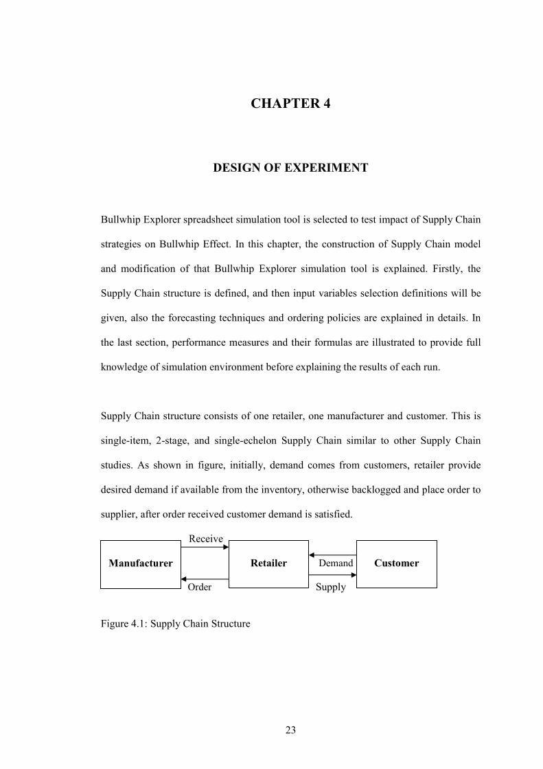
Supply Chain structure consists of one retailer, one manufacturer and customer. This is

single-item, 2-stage, and single-echelon Supply Chain similar to other Supply Chain

studies. As shown in figure, initially, demand comes from customers, retailer provide

desired demand if available from the inventory, otherwise backlogged and place order to

supplier, after order received customer demand is satisfied.

Receive

Demand

Order Supply

Figure 4.1: Supply Chain Structure

Manufacturer

Retailer

Customer

24

4.1 Input Module The inputs are the most important parts of the simulation tool. Because all selected

factors are defined here to test their effects on performance measures. As mentioned

before there are eleven different factors. These are; forecasting technique, demand

distributions, ordering cost, backorder cost, holding cost, demand mean, variance,

number of forecast periods, lead time and finally service levels. All these factors are

determined as a result of hard and detailed research on Supply Chain literature. And it is

quite clear that, this study becomes the unique study in literature which combines all

defined and undefined factors in a single study to test their effects on Supply Chain

performance.

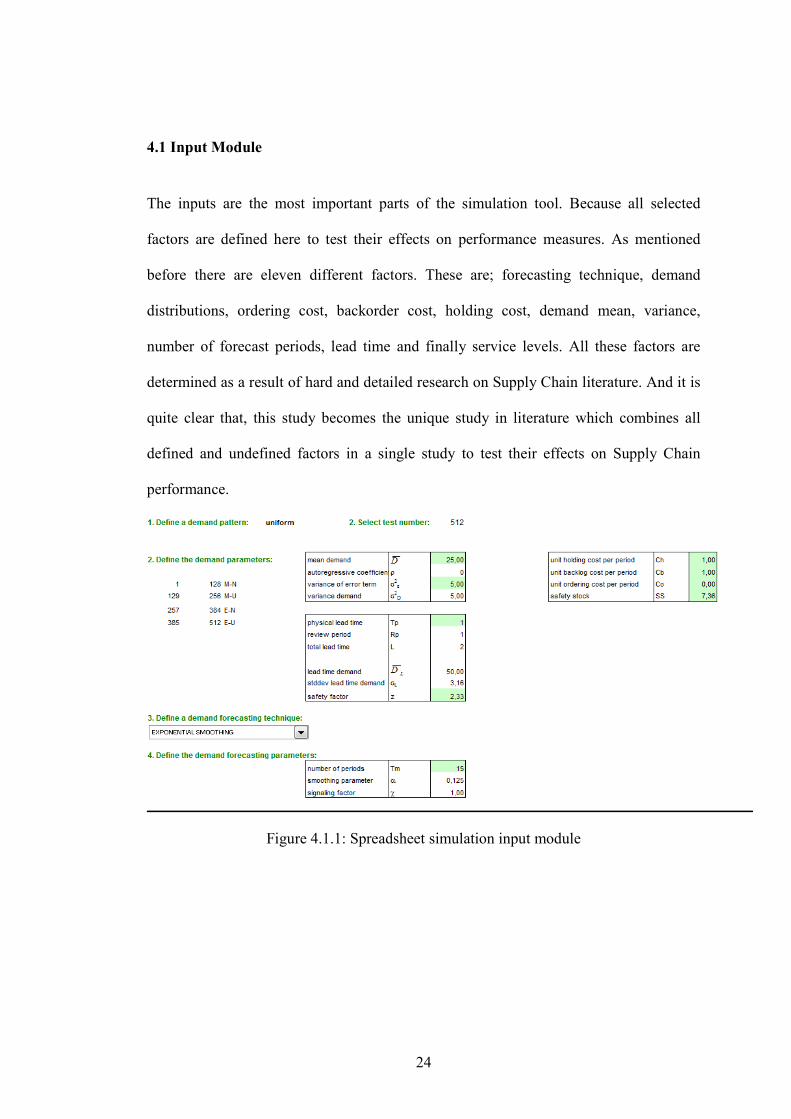
Figure 4.1.1: Spreadsheet simulation input module

25

As shown in figure 4.1.1. all factors values are defined in input section of simulation

tool. For example first the demand parameter value needs to be entered (i.e. Mean

Demand). It is the average demand represented as D .

In original bullwhip explorer tool, the mean demand value is taken as a constant value.

But, in this study since it is one of the factors which could have an impact on Bullwhip

Effect, two different, mean demand values are chosen to show it’s high and low

conditions. 10 represent the low and 25 represents the high levels of this factor.

Following input value and factor is the demand variance. It is represented as σ2 D and

calculated by the formula shown below;

2

Dσ = σ2

V / (1 – ρ2

)

ρ: autoregressive coefficient

In bullwhip explorer it is chosen as a constant value. In this study, 1 show low and 5

shows the high level of this factor.

In bullwhip explorer file demand type can be chosen as independently and identically

distributed (IID) or AR demand types. But here it is assumed as independent and

identically distributed demand. But it is known that for independent and identically

distributed demand autoregressive coefficient ρ is and variance of error term σ2

V are

equal to zero

26

In this study instead of demand type, demand distribution is selected as a factor which

can have an impact on Bullwhip Effect. So, two different demand distributions; normal

and uniform are tested to see their effects on Supply Chain performance.

In bullwhip explorer the demand values are randomly generated according to demand

type and each different click on simulate button will be result in different random

demand values for each 500 periods.

The random number generation should be made according to different demand

distributions and different demand mean and variances. Also for each different click on

simulate button; demand pattern should not be changed while the other input values

were same.

By this way, all factors effect is tested in the same simulation environment. For this

reason a separate demand excel file is prepared to be ready to use in simulation tool. In

demand excel file, there are eight different random demand numbers generation list for

each different demand distribution; normal and uniform and for each high and low

values of mean and variance. To have valid results, all these eight demand values are

tested using ARENA Input analyzer. Input analyzer result is shown in appendix in

figures 1-8. For example random demand number generated with normal distribution

with mean 10 and variance 1 tested in input analyzer and it also resulted as normal

distribution with mean 10 and variance 1.

27

To sum up, in simulation tool when demand mean and variance is changed according to

the factor combinations in input excel file, suitable random demand values are taken

from that excel file and when a new click made on simulate button, these demand values

will not be changed while the mean variance and demand distribution were same.

The other input value and factor is physical lead time (Tp). It is the lead time caused by

transportation lag or any other material delivery delays. In bullwhip explorer user can

choose any constant value to the simulation tool. But increase and decrease of lead time

directly affects Bullwhip Effect. Several studies made to see the effect of lead time on

Bullwhip Effect. To compare with existing literature, in this study lead time is one of the

factors and it is values are determined as 1 for low and 5 for high level of this factor.

Review period Rp is the position which shows the time to review inventory position. In

bullwhip explorer it is assumed as 1 which means inventory position is reviewed every

period. Also most of the other Supply Chain studies assumed the review period is one.

The reason for that can be the simplification of the study and usage of existing Bullwhip

Effect formula with same number of orders and demand in each period. Because when

review period is different from one, in some period orders can be zero even there is

demand. And different data series for demand and orders values could cause some

mistakes or not correct variance of orders and demand comparison for Bullwhip Effect.

But in this study, review period is selected as an important factor which can affect

Bullwhip Effect and 1 and 5 is selected for its low and high levels. The existing

Bullwhip Effect formula in literature is not given correct result when review period is

28

high. For this reason the known Bullwhip Effect formula is needs to be improved in this

study to be able to use in every different situation and be more close to real life by

different review periods. Details for Bullwhip Effect formula will be explained in

performance measure section.

The input section is continued with total lead time (L),

L = Rp + Tp

Average lead time demand (DL) and standard deviation (σL) are calculated by the

following formulas;

DL = L * D

σL = 2* DL σ

Another important input is safety stock which is the minimum amount that should be

held in inventory which and is calculated by the formula shown below. It has an

important role for the decision of ordering amount and time.

Safety stock = ss = z * σRp+Tp

In safety stock calculation safety factor (z) is the key element. For this reason, safety

factor should be one of the factors needed to test its impact on Bullwhip Effect. Two

different service levels are selected as 80% and 90%, so their corresponding z values,

0.842 and 2.327 are defined as low and high levels of safety factor.

29

There are different forecasting techniques for future demand calculations. Since demand

is an important element of Supply Chain, the demand forecasting technique could be

effective for Bullwhip Effect. In literature many similar studies made discussions for the

demand forecasting effects on bullwhip. To be consistent with literature, in this study

moving average and exponential smoothing are selected as two different types of

demand forecasting techniques.

Demand forecasting techniques are determined. Now, the forecasting parameters should

be defined. Most common elements of forecasting are number of periods (N) for moving

average and smoothing parameter (α ) for exponential soothing. The high and low level

for number of period is determined as 7 and 15.

As seen in the following formula, smoothing parameter calculation is done by using

number of forecast periods value, for this reason instead of taking in to account as two

different forecasting parameters, only number of forecast period is selected as factor

which can affect Supply Chain.

1

2

+=N

α

Costs are the other important input values for this simulation model. Most of the

previous Bullwhip Effect studies not taken into account the cost structure in to their

models.

30

But in this thesis, three different cost values are selected and two different values for

each of them are determined to see their impacts on performance measures.

The cost structure components are explained in the following definitions;

• Holding (or carrying) costs: Costs for capital, taxes, insurance, etc. (Dealing

with storage and handling)

• low level: 0,1 and high level: 1 TL/unit-period

• Ordering costs (services & manufacturing): Costs of someone placing an order,

etc.

• low level: 0,1 and high level: 1 TL/unit-period

• Shortage (backordering) costs: Costs of cancel or postpone an order, customer

goodwill, etc.

• low level: 10 and high level: 100 TL/order

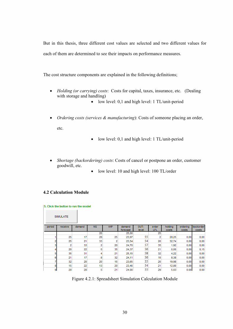
4.2 Calculation Module

Figure 4.2.1: Spreadsheet Simulation Calculation Module

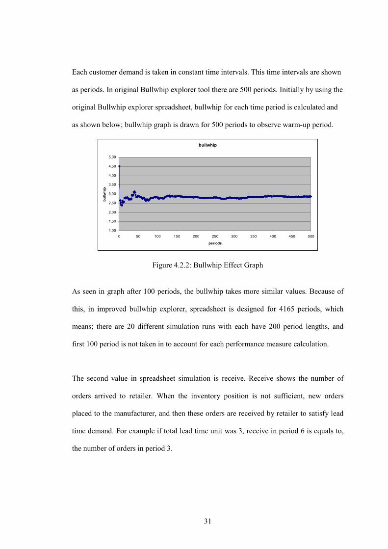
31

Each customer demand is taken in constant time intervals. This time intervals are shown

as periods. In original Bullwhip explorer tool there are 500 periods. Initially by using the

original Bullwhip explorer spreadsheet, bullwhip for each time period is calculated and

as shown below; bullwhip graph is drawn for 500 periods to observe warm-up period.

bullwhip

1,00

1,50

2,00

2,50

3,00

3,50

4,00

4,50

5,00

0 50 100 150 200 250 300 350 400 450 500

periods

bullwhip

Figure 4.2.2: Bullwhip Effect Graph

As seen in graph after 100 periods, the bullwhip takes more similar values. Because of

this, in improved bullwhip explorer, spreadsheet is designed for 4165 periods, which

means; there are 20 different simulation runs with each have 200 period lengths, and

first 100 period is not taken in to account for each performance measure calculation.

The second value in spreadsheet simulation is receive. Receive shows the number of

orders arrived to retailer. When the inventory position is not sufficient, new orders

placed to the manufacturer, and then these orders are received by retailer to satisfy lead

time demand. For example if total lead time unit was 3, receive in period 6 is equals to,

the number of orders in period 3.

32

Demand is the random customer demand values which are assumed to be uniform or

normally distributed with mean demand and variance demand as defined in input

section.

NS is the net stock quantity in each period. Net stock formula is given below. According

to the formula, net stock of sixth period is equals to net stock of fifth period plus order

placed in third period minus sixth period’s customer demand.

NSt = NSt-1 + Ot-(Tp+1) – Dt

WIPt is the work in process inventory in period t. It equals to the work in process

inventory of previous period plus orders placed previous period minus total lead time

periods ago order value.

WIPt = WIPt-1 + Ot-1 – Ot-(Tp+1)

Demand forecast can be done by using different forecasting techniques. In this study, as

explained in previous section moving average and exponential smoothing techniques are

used. In input part user can select desired forecasting technique from the list. Two

forecasting methods and demand forecast calculations are explained in the following

section.

Moving average method; demand forecast is measured by taking the average of

determined past periods (Tm) actual demand values. Each next forecast removes

demand in the oldest period and replaces it with the demand in the most recent period;

so, the data in the calculation "moves" over time.

33

Exponential smoothing is the other forecasting technique used in this study. In this

method demand forecast is calculated by using forecast error to correct the previous

smoothed value (α).

)( 11 −

∧

−

∧∧

−+= tttt DDDD α

Inventory replenishment rule applied in this study is the period review system. The other

type of replenishment rule is fixed order quantity system. In fixed order quantity model,

quantity of ordered product is same but order time intervals are varies. But in periodic

order systems, the orders are made in specified time intervals with different order

amounts. As mentioned before, in periodic order system order quantities are change in

each period.

The calculation of order period can be done with different ordering policies. In literature

there are different researchers made studies for effect of inventory policies on Bullwhip

Effect. In this study it is decided to run the simulation model according to two different

inventory policies to observe their effect on Supply Chain performance measures.

First chosen inventory policy is lot for lot policy since it is most widely used in real life

and the second one is standard periodic review order-up-to policy since it is most widely

used in Bullwhip Effect literature.

m

iTm

i

itt TDD /0

= ∑

−

=−

∧

34

Lot for lot policy is most common in industries because of its practical and easy

application. If the forecasted demand (Ft) at the beginning of an order period is k with a

lead time of τ periods the order amount in lot for lot ordering policy is calculated by the

following formula:

Every k-period’s lot for lot order size = ∑=

++

k

i

itF1

τ

Second ordering policy is standard order up to level policy. In standard periodic review

order-up-to policy, the inventory position IPt is calculated at the end of every review

period Rp and compared with an order-up-to (OUT) level St. IPt is the addition of the net

stock NSt and the inventory on order WIPt.

The OUT level St is calculated by summation of the forecasted average lead time

demand and a safety stock. Forecasted lead time demand is the multiplication of total

lead time by forecasted demand (by using moving average or exponential smoothing).

The OUT level (St) is calculated with the following formula.

+=∧t

Lt DS Safety Stock

∧t

LD : forecasted average lead time demand

Out level shows the target inventory level. For this reason in each review period new

order should made to raise the inventory quantity to out-level. Order amount is

calculated by the following formula; which shows the difference of out level from

inventory position.

Ot = St – (NSt + WIPt)

35

The last calculations in simulation are done to calculate cost structure. There are three

different cost values. Inventory holding cost ( h

tC ), ordering cost ( o

tC ) and backorder

costs ( b

tC ). The calculation of each cost is made according to the following formulas.

Holding cost, where NSt >=0

th

h

t NSCC *=

Backorder cost, where NSt <=0

tb

b

t NSCC *=

Ordering cost, where Ot ≠ 0

1*oo

t CC =

The all input values and calculations are defined with their formulas. The last part of

simulation is the calculation of performance measures with given input values. The

performance measures and their formulas are explained in next section.

4.3 Output Module:

In original bullwhip explorer there are only four different performance measures;

bullwhip, net stock amplification, customer service level and fill rate. But in this study,

different performance measures are used to have more effective results and

recommendation for each factor’s effect.

Bullwhip is the main performance measure in simulation. It is calculated by the

following formula, which says division of variance of orders to variance of demand. As

36

Bullwhip measurement equal to one means there is no variance amplification, demand

variance and order variances are same. But if bullwhip is bigger than one, it means that

Bullwhip Effect is present and solution to reduce them should be investigated. In

literature the bullwhip is defined as in the formula shown below;

Bullwhip = 2

2

demand

orders

σσ

But as explained in input section this formula is not applicable when review periods is

different form 1. Because in some periods there could be no orders so, the number of

orders and demand would not be in same amount and this would cause wrong variance

comparison. For this reason Bullwhip Effect formula is improved to be ready to use in

all different review period situations.

The improved Bullwhip Effect formula is generated by adapting coefficient of variation

formula. It represents the ratio of the standard deviation to the mean, and it is a useful

statistic for comparing the degree of variation from one data series to another, even if the

units or means are drastically different from each other.

Coefficient of Variation µσ

=

So, the improved Bullwhip Effect formula is generated as shown in the following

formula:

37

Bullwhip Effect = demanddemand

ordersorders

µσµσ

/

/

Net stock amplification is the second performance measure which also used in original

bullwhip explorer simulation. It shows the increase in inventory variance, and gives an

idea about customer service level, by illustrating if there is a need for more safety stock.

The original formula is shown below;

NSAmp = 2

2

demand

netstock

σσ

Similar to Bullwhip Effect the net stock amplification formula also improved to get valid

results in different input values, but as a remark net stock is used as a performance

measure in spreadsheet simulation but the analysis design for the factors effect on net

stock amplification is not discussed in this study. The improved formula which used in

simulation is shown below;

NSAmp = demanddemand

netstocknetstock

µσµσ

/

/

Final output values are calculated for cost structure. These can be calculated as;

Total holding cost = summation of all holding cost for each 200 periods.

Total backorder cost = summation of all backorder cost for each 200 periods.

Total ordering cost = summation of all ordering cost for each 200 periods.

Total cost = summation of all holding, ordering and backorder cost for each 200 periods.

38

In this section, all input values and calculations for simulation model are explained in

details. The simulation spreadsheet is finalized according to these defined values. The

input excel file for lot for lot and for standard out policy are given in CD, in this file all

factor combinations are listed with their corresponding output values, also demand

values are given in CD with two separate excel file; one for lot for lot and one for

standard out policy. Finally Bullwhip Effect simulation spreadsheets are prepared and

simulation for standard out policy is shown in figure 9 and spreadsheet simulation for lot

for lot for is shown in figure 13.

When user open related excel files and run the simulation, all factor combinations are

automatically written to the simulation model and related input and output values are

respectively recorded to predetermined file destinations. As a result of this automated

simulation study all factor combinations results can be calculated in 15-20 minutes.

All input values and output values are ready, next step should be the analysis and

explanation of these results. Minitab statistical analysis software is used to make these

analyses and to get valid results for the effects of factors on Supply Chain. Details and

explanation of the analysis are explained in the following chapter.

39

CHAPTER 5

EXPERIMENTAL ANALYSIS

Minitab is statistical analysis software for the use of academic or business statistical

researches. In this thesis the aim is the identification of eleven different factors effect on

Supply Chain performance measure such as Bullwhip Effect.

There are two different simulation models, one of them is for lot for lot and the other

one is for standard out policy. Their analyses are made separately but the same design of

experiment is used since the cause affect structure is the same for both models.

Eleven different factors impact on Bullwhip Effect is analyzed using general full

factorial design of experiments method. First the levels of each factor is defined, all

factors have two levels in this study. Then the design is prepared for 4 replicate.

Replication number should be selected at least two to be able to estimate interaction

effects, therefore it is selected as 4, for this study. Then, Minitab is resulted with 8192

rows for each different factor combinations.

The desired response value should be written for each row. For this reason each

simulation model is run for 8 times, and average of twenty output values for each single

40

simulation is recorded in different excel files, so 8192 different performance measure for

each factor combinations of simulation models are prepared for the use of general full

factorial analysis.

Figure 10, 11 and 12 shows the Minitab results for standard out policy and figure 14, 15

and 16 shows the Minitab results for lot for lot policy. When pre-calculated bullwhip

values are entered to Minitab worksheet then, analyze factorial design button is chosen

to see these results of the analysis. To better explain the results of defined analysis

methods; additional graphs are selected in Minitab.

In this study, for the analysis of each simulation models with general full factorial

design; analysis of variance, normal plot, main effects plot, interaction plot, pareto chart

and normal effects plots are selected to better explain the results of the analysis

In the following section, effects of all factors on Bullwhip Effect for standard out policy

and for lot for lot policy are explained according to general full factorial and ANOVA

results in addition to the demonstration of related graphs.

41

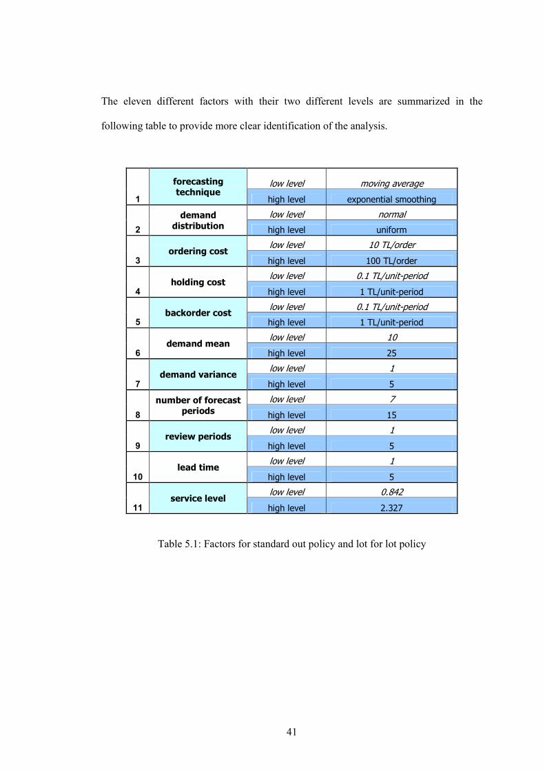
The eleven different factors with their two different levels are summarized in the

following table to provide more clear identification of the analysis.

1

forecasting technique

low level moving average

high level exponential smoothing

2

demand

distribution

low level normal

high level uniform

3 ordering cost

low level 10 TL/order

high level 100 TL/order

4 holding cost

low level 0.1 TL/unit-period

high level 1 TL/unit-period

5 backorder cost

low level 0.1 TL/unit-period

high level 1 TL/unit-period

6 demand mean

low level 10

high level 25

7 demand variance

low level 1

high level 5

8

number of forecast periods

low level 7

high level 15

9 review periods

low level 1

high level 5

10 lead time

low level 1

high level 5

11 service level

low level 0.842

high level 2.327

Table 5.1: Factors for standard out policy and lot for lot policy

42

5.1 Analysis for Standard Out Policy:

The experiment is designed for 11 factors with two levels. The experiment is handled

with general full factorial design. Before explaining the result, the model adequacy is

checked by the following statistical analysis.

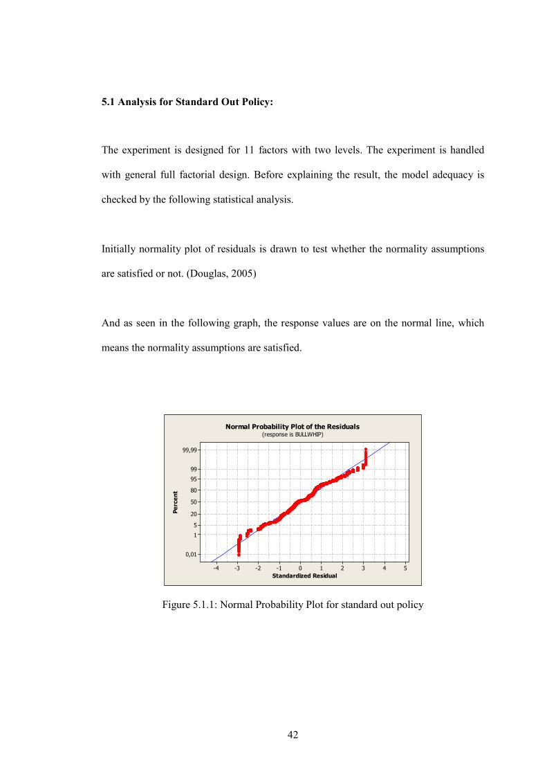
Initially normality plot of residuals is drawn to test whether the normality assumptions

are satisfied or not. (Douglas, 2005)

And as seen in the following graph, the response values are on the normal line, which

means the normality assumptions are satisfied.

Standardized Residual

Percent

543210-1-2-3-4

99,99

99

95

80

50

20

5

1

0,01

Normal Probability Plot of the Residuals(response is BULLWHIP)

Figure 5.1.1: Normal Probability Plot for standard out policy

43

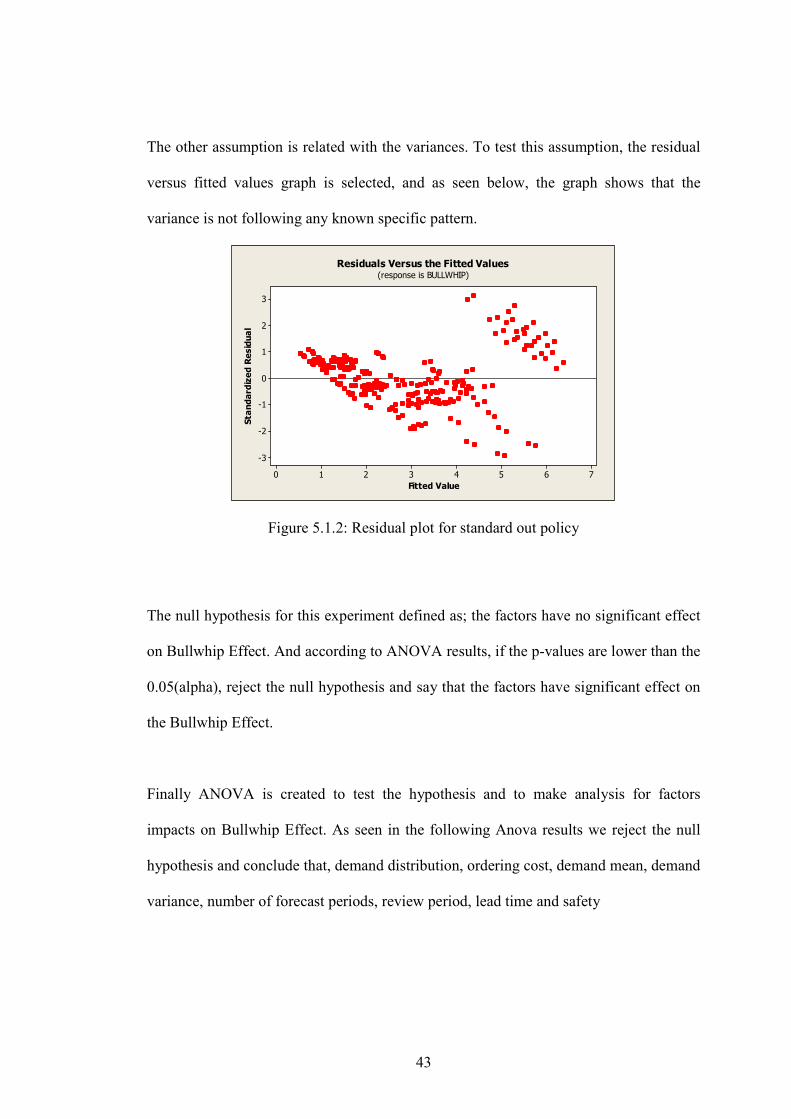
The other assumption is related with the variances. To test this assumption, the residual

versus fitted values graph is selected, and as seen below, the graph shows that the

variance is not following any known specific pattern.

Fitted Value

Standardized Residual

76543210

3

2

1

0

-1

-2

-3

Residuals Versus the Fitted Values(response is BULLWHIP)

Figure 5.1.2: Residual plot for standard out policy

The null hypothesis for this experiment defined as; the factors have no significant effect

on Bullwhip Effect. And according to ANOVA results, if the p-values are lower than the

0.05(alpha), reject the null hypothesis and say that the factors have significant effect on

the Bullwhip Effect.

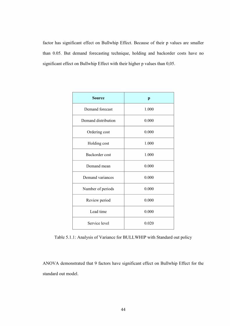
Finally ANOVA is created to test the hypothesis and to make analysis for factors

impacts on Bullwhip Effect. As seen in the following Anova results we reject the null

hypothesis and conclude that, demand distribution, ordering cost, demand mean, demand

variance, number of forecast periods, review period, lead time and safety

44

factor has significant effect on Bullwhip Effect. Because of their p values are smaller

than 0.05. But demand forecasting technique, holding and backorder costs have no

significant effect on Bullwhip Effect with their higher p values than 0,05.

Source p

Demand forecast 1.000

Demand distribution 0.000

Ordering cost 0.000

Holding cost 1.000

Backorder cost 1.000

Demand mean 0.000

Demand variances 0.000

Number of periods 0.000

Review period 0.000

Lead time 0.000

Service level 0.020

Table 5.1.1: Analysis of Variance for BULLWHIP with Standard out policy

ANOVA demonstrated that 9 factors have significant effect on Bullwhip Effect for the

standard out model.

45

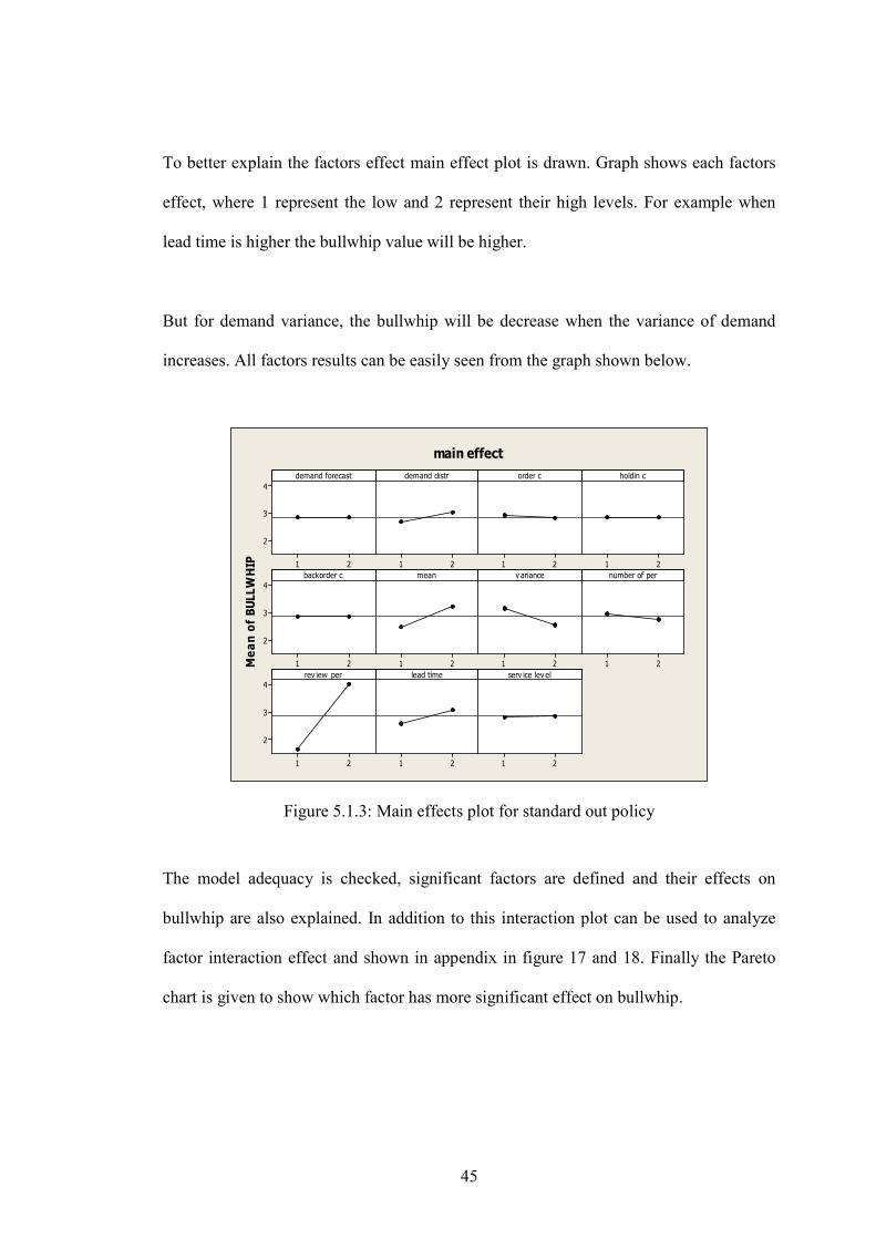
To better explain the factors effect main effect plot is drawn. Graph shows each factors

effect, where 1 represent the low and 2 represent their high levels. For example when

lead time is higher the bullwhip value will be higher.

But for demand variance, the bullwhip will be decrease when the variance of demand

increases. All factors results can be easily seen from the graph shown below.

Mean of BULLWHIP 21

4

3

2

21 21 21

21

4

3

2

21 21 21

21

4

3

2

21 21

demand forecast demand dıstr order c holdin c

backorder c mean v ariance number of per

rev iew per lead time serv ice lev el

main effect

Figure 5.1.3: Main effects plot for standard out policy

The model adequacy is checked, significant factors are defined and their effects on

bullwhip are also explained. In addition to this interaction plot can be used to analyze

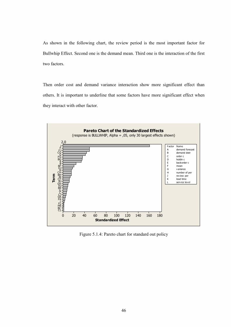
factor interaction effect and shown in appendix in figure 17 and 18. Finally the Pareto

chart is given to show which factor has more significant effect on bullwhip.

46

As shown in the following chart, the review period is the most important factor for

Bullwhip Effect. Second one is the demand mean. Third one is the interaction of the first

two factors.

Then order cost and demand variance interaction show more significant effect than

others. It is important to underline that some factors have more significant effect when

they interact with other factor.

Term

Standardized Effect

CLBCHKFLL

FKGKCJCJLBKHJGHBJCFJKBHCHHGJBFBK

BGFGG

CGFJFJ

180160140120100806040200

2,0Factor

holdin c

E backorder c

F mean

G v ariance

H number of per

J

Name

rev iew per

K lead time

L serv ice lev el

A demand forecast

B demand dıstr

C order c

D

Pareto Chart of the Standardized Effects(response is BULLWHIP, Alpha = ,05, only 30 largest effects shown)

Figure 5.1.4: Pareto chart for standard out policy

47

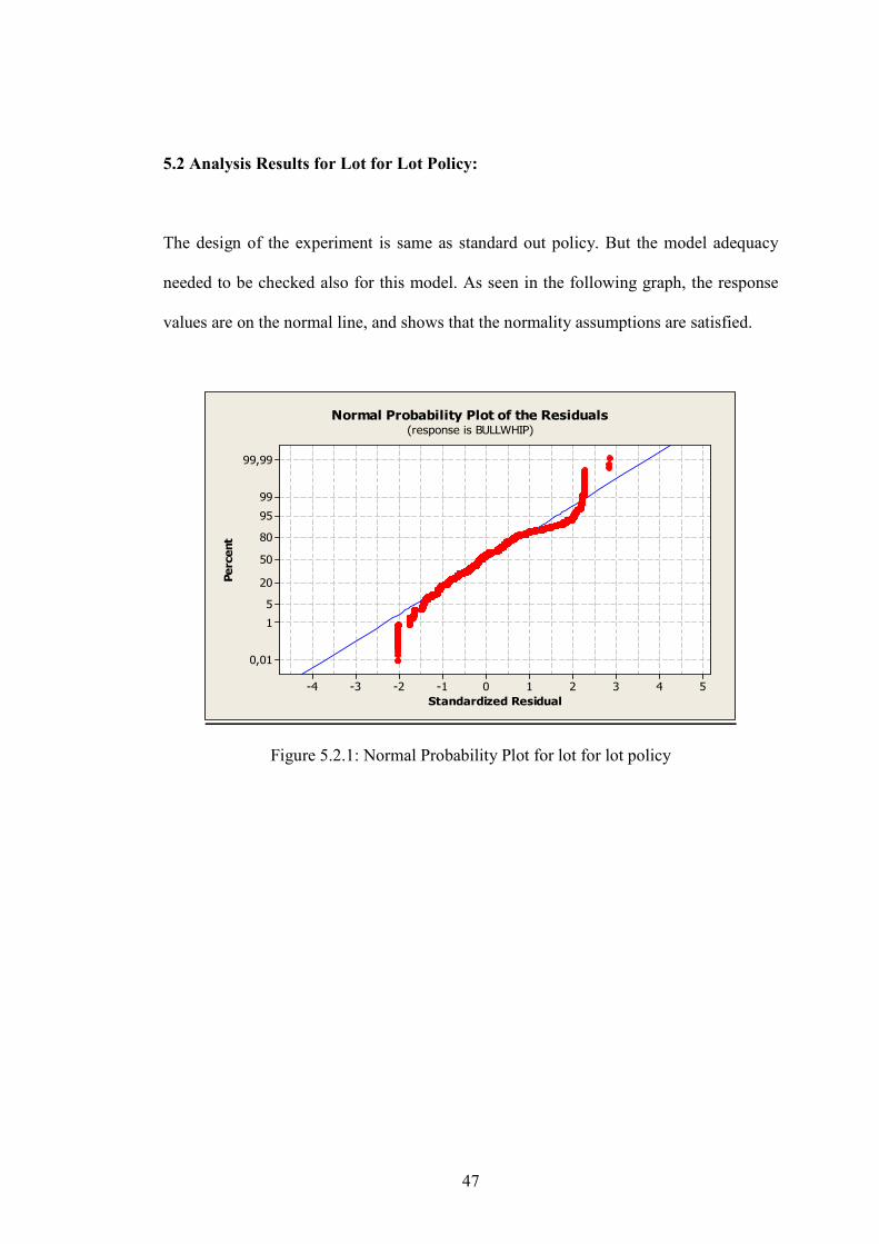
5.2 Analysis Results for Lot for Lot Policy:

The design of the experiment is same as standard out policy. But the model adequacy

needed to be checked also for this model. As seen in the following graph, the response

values are on the normal line, and shows that the normality assumptions are satisfied.

Standardized Residual

Percent

543210-1-2-3-4

99,99

99

95

80

50

20

5

1

0,01

Normal Probability Plot of the Residuals(response is BULLWHIP)

Figure 5.2.1: Normal Probability Plot for lot for lot policy

48

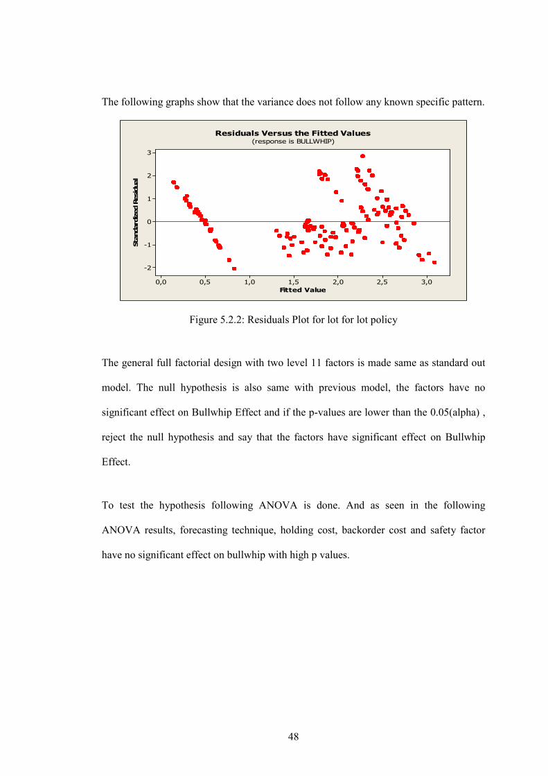
The following graphs show that the variance does not follow any known specific pattern.

Fitted Value

Standardized Residual

3,02,52,01,51,00,50,0

3

2

1

0

-1

-2

Residuals Versus the Fitted Values(response is BULLWHIP)

Figure 5.2.2: Residuals Plot for lot for lot policy

The general full factorial design with two level 11 factors is made same as standard out

model. The null hypothesis is also same with previous model, the factors have no

significant effect on Bullwhip Effect and if the p-values are lower than the 0.05(alpha) ,

reject the null hypothesis and say that the factors have significant effect on Bullwhip

Effect.

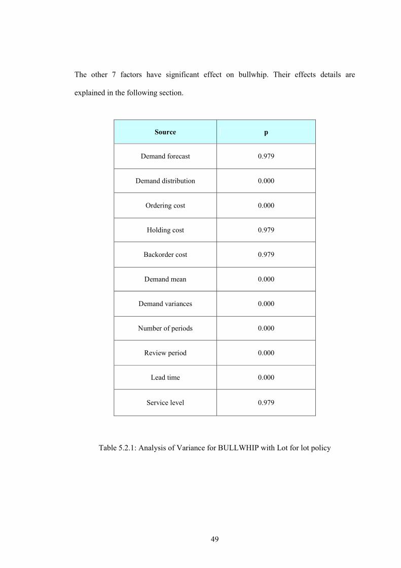
To test the hypothesis following ANOVA is done. And as seen in the following

ANOVA results, forecasting technique, holding cost, backorder cost and safety factor

have no significant effect on bullwhip with high p values.

49

The other 7 factors have significant effect on bullwhip. Their effects details are

explained in the following section.

Source p

Demand forecast 0.979

Demand distribution 0.000

Ordering cost 0.000

Holding cost 0.979

Backorder cost 0.979

Demand mean 0.000

Demand variances 0.000

Number of periods 0.000

Review period 0.000

Lead time 0.000

Service level 0.979

Table 5.2.1: Analysis of Variance for BULLWHIP with Lot for lot policy

50

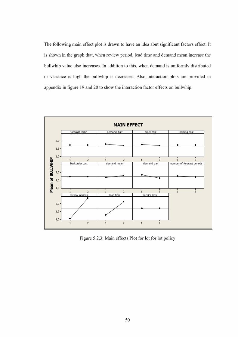
The following main effect plot is drawn to have an idea abut significant factors effect. It

is shown in the graph that, when review period, lead time and demand mean increase the

bullwhip value also increases. In addition to this, when demand is uniformly distributed

or variance is high the bullwhip is decreases. Also interaction plots are provided in

appendix in figure 19 and 20 to show the interaction factor effects on bullwhip.

Mean of BULLWHIP 21

2,0

1,5

1,0

21 21 21

21

2,0

1,5

1,0

21 21 21

21

2,0

1,5

1,0

21 21

forecast techn demand distr order cost holding cost

backorder cost demand mean demand v ar number of forecast periods

rev iew periods lead time serv ice lev el

MAIN EFFECT

Figure 5.2.3: Main effects Plot for lot for lot policy

51

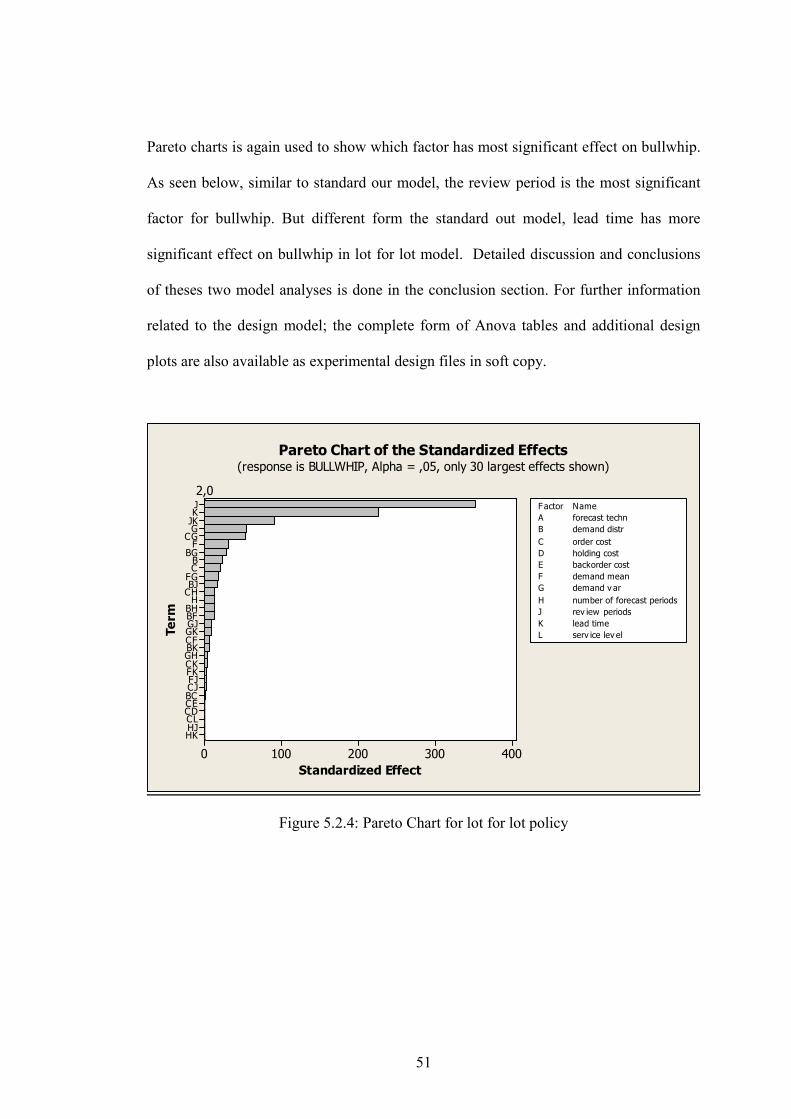
Pareto charts is again used to show which factor has most significant effect on bullwhip.

As seen below, similar to standard our model, the review period is the most significant

factor for bullwhip. But different form the standard out model, lead time has more

significant effect on bullwhip in lot for lot model. Detailed discussion and conclusions

of theses two model analyses is done in the conclusion section. For further information

related to the design model; the complete form of Anova tables and additional design

plots are also available as experimental design files in soft copy.

Term

Standardized Effect

HKHJCLCDCEBCCJFJFKCKGHBKCFGKGJBFBHH

CHBJFGCB

BGF

CGGJKKJ

4003002001000

2,0Factor

holding cost

E backorder cost

F demand mean

G demand v ar

H number of forecast periods

J

Name

rev iew periods

K lead time

L serv ice lev el

A forecast techn

B demand distr

C order cost

D

Pareto Chart of the Standardized Effects(response is BULLWHIP, Alpha = ,05, only 30 largest effects shown)

Figure 5.2.4: Pareto Chart for lot for lot policy

52

CHAPTER 6

CONCLUSION

The aim of this thesis was the investigation of different Supply Chain strategies on

Bullwhip Effect. In literature there are similar studies related to Bullwhip Effect.

Different from other studies, this thesis combined and analyzed all factors effects on

Bullwhip.

The first important decision was related to the selection of factors. Hence, detailed

literature survey is made in addition to real case observations. According to this survey,

eleven factors are determined, and each factor is tested with its two different levels. First

factor is selected as demand forecasting, and two different forecasting techniques;

moving average and exponential smoothing is tested for each Supply Chain strategies.

Second factor was related to demand distribution; normal and uniform distribution is

chosen to test this factor. Also, demand mean, demand variance, ordering, holding and

backorder costs, number of forecast periods, lead time, review period and service level

are the other factors and each of them has two different levels defined as high and low.

The last but most important factor is the ordering policy. Decision for two different

types of ordering policy was another hard topic. Standard out policy selected, because of

53

it is most used ordering policy in Bullwhip Effect literature and Lot for lot ordering

policy is selected since it is most widely used ordering policy in real cases.

As a result of 11 factors and two different levels for each of them, there are 2048

different factor combinations. In addition to this, all of them should be tested with two

different ordering policies. To sum up, there are 2048 different Supply Chain strategies

for standard out policy and 2048 strategies for lot for lot policy to test the impact on

Bullwhip Effect.

It’s obvious that the scope of this study is extensive. The most suitable methodology for

this type of research as discussed in literature is Simulation technique. But none of the

available simulation tools were suitable for this type of research. Therefore, another step

of this study was the generation of a new Supply Chain simulation tool.

New simulation tool is designed with Ms Excel spreadsheets with the use of Macros.

The tool can be downloaded and used for any type of Supply Chain research and/or

industrial studies. To make more useful and accurate simulation tool, in addition to

Bullwhip Effect, other performance measures, such as; net stock amplification, ordering,

holding, backorder and total costs are also added as other output modules of the

simulation. Additionally, this tool is user friendly and can be easily modified for

different type of Supply Chain structures.

As said in the beginning the aim of this thesis is to test the factors effect on bullwhip.

So, the quantification of the Bullwhip Effect was very important. But while making

54

simulation for different review periods, it was observed that formula gives misleading

results.

Because in literature Bullwhip Effect defined as, the rate of variance of orders to

variance of demand. So, in different review periods, demand occurs in each period but

orders are not same in each period. This causes wrong variance comparisons and gives

wrong Bullwhip Effect measures. To solve this problem and prevent wrong results, the

Bullwhip Effect formula was improved in this study. Coefficient of variation formula

adapted to defined Bullwhip Effect formula, and it’s proven that this formula is more

accurate and valid for all different Supply Chain studies.

As a result of simulation, the Bullwhip Effect measures are calculated for each different

ordering policy. To make objective conclusion, each simulation result is analyzed by

Minitab statistical software Packages.

The design of experiment is made by factorial design with two levels. The analysis

results were valuable to make comments and suggestion for the improvements of

Bullwhip Effect.

For standard out policy, it is proven that demand distribution, ordering cost, demand

mean, demand variance, number of forecast periods, review period, lead time and safety

factor have significant effect on Bullwhip Effect. And review period is the most

important factor. To reduce the Bullwhip Effect, review period should be reduced too.

55

For lot for lot policy, demand distribution, ordering cost, demand mean, demand

variance, number of forecast periods, review period, and lead time have significant

effect on bullwhip. Review period is again the most important factor for this policy.

As seen here, factors can have similar effects in different ordering policies or diverse

Supply Chain strategies. But there is also some common results as when review period is

low bullwhip will also be low and same conclusion can be made for lead time too.

But in real life the situations are different. Companies sometimes doesn’t have chance to

change review period or lead time. For this reason this study is made for all different

factor combination. This means, may be Supply Chain member doesn’t have capability

to change one factor, but it’s proven and shown that there should be some alternative

solution to reduce bullwhip. In addition to this, the provided simulation tool can be used,

to test which Supply Chain strategy can be selected according to predetermined factor

limitations. Beside that, the effect of selected factors on cost measure or net stock

amplification can be other selection criteria for the solution of Supply Chain problem.

As a conclusion, this study managed to detect significant factors that effect Bullwhip

and shows alternative solution strategies of Bullwhip Effect. Additionally new Supply

Chain Simulation tool and improved Bullwhip Effect formula is illustrated to motivate

better and improved studies in Supply Chain literature and solutions for real case

problems.

56

REFERENCES

[1] Beamon B. M. (1998), “Supply chain design and analysis: Models and

methods,” International Journal of Production Economics, 55:281-294.

[2] Cachon G.P. (1999), “Quantitative models for supply chain management,”

Kluwer Academic Publishers, Boston, 111–146.

[3] Camm T., E. Chorman, F.A. Dill, J.R. Evans, D.J. Sweeney and G.W. Wegryn

(1997), “Blending OR/MS judgment and GIS: Restructuring P&G's supply

chain,” International Journal of Production Economics, 27:128–142.

[4] Cantor, D.E. and J.R. MacDonald (2008), “Decision making in the supply chain:

Examining problem solving approaches and information availability,” Journal of

Operations Managements, 26:461-556.

[5] Chen F., Drezner Z., J. Ryan and D. Simchi-Levi (1998), “Quantifying the

bullwhip effect: The impact of forecasting, lead times and information,”

Management Science, 46:436-443.

[6] Cohen M. and L. Lee (1989), “Resource deployment analysis of global

manufacturing and distribution networks,” Journal of Manufacturing and

Operations Management, 2:81–104.

57

[7] Cohen M. and S. Moon (1990), “Impact of production scales economies,

manufacturing complexity and transportation cost on supply chain facility

network,” Journal of Manufacturing and Operations Management,

3:269-292.

[8] Cooper M. J., D.M. Lambert and J.D. Pagh (1997), “Supply chain management:

more than a new name for logistics,” The International Journal of Logistics

Management, 8:1–13.

[9] Dejonckheere J., S. Disney, M. Lambrecht and D. R. Towill (2003), “Measuring

the bullwhip effect: A control theoretic approach to analyse forecasting induced

bullwhip in order-up-to policies,” European Journal of Operational Research,

147:567-590.

[10] Douglas C. (2005), “Design and analysis of experiments,” John Wiley & Sons,

New York. America.

[11] Enns S.T. and P. Suwanruji (2003), “A simulation test bed for production and

supply chain modeling,” International Journal of Production Economics,

2:1174-1182.

[12] Forrester J. (1958), “Industrial dynamics, a major breakthrough for decision

bakers,” Harvard Business Review, 36:67-96.

58

[13] Harrell C.R. and K. Tumay (1994), “Simulation of manufacturing and service

system,” IE Management. Press, 5:114-121.

[14] Ishii K., K. Takahafhi and R. Muramatsu (1988), “Integrated production

inventory and distribution system,” International Journal of Production Research

26:473-482.

[15] Karabakal N., A. Gunal and W. Ritchie (2000), “Supply chain analysis of

volkswagen of America,” International Journal of Computer Integrated

Manufacturing, 4:46–55.

[16] Karmarkar A. and N.R. Patel (1977), “The one-period, n-location distribution

problem,” Naval Research Logistics Quarterly, 24:559–575.

[17] Lee H., P. Padmanabhan and S. Whang (1997), “Information distortion in a

supply chain: The bullwhip effect,” Management Science, 5:546-58.

[18] Liu J., J. Wang, Y. Chai and Y. Liu (2004), “Easy-sc: A Supply chain

simulation tool,” Simulation Conference, 2:1373-1378.

[19] Machuca J.A.D. and R. P. Barajas, R.P. (1997) “A computerized network

version of the beer game via the internet,” Systems Dynamics Review,

13:323-340.

59

[20] Manyem P. V. and Santoz B. (1999) “Factors that influence the bullwhip

Effect and its Impacts on profitability: A simulation study on supply chain,”

Management Science, 43:546-556.

[21] Min H. and G. Zhou (2002) “Supply Chain modeling: past, present, future”,

Computers and Industrial Engineering, 43:231–249.

[22] Nozick L.K and M.A. Turnquist (2001), “Inventory, transportation, service

quality and the location of distribution centers,” European Journal of Operational

Research, 129:362–371.

[23] Sezen B. (2004), “Tedarik zincirinde stok yönetimi problemleri için elektronik

tablolar yardımı ile simülasyon uygulaması,” Yönetim ve Ekonomi, 12:219-230.

[24] Simchi-Levi D. and P. Kaminsky (2000), “Designing and managing the supply

chain: concepts, strategies, and case studies,” Irwin McGraw-Hill.

[25] Stevens G.C. (1989), “Integrating the supply chain,” International Journal of

Physical Distribution and Materials Management, 19:3–8.

[26] Swaminathan M. and C. Tayur (1999), “Stochastic programming models for

managing product variety,” Quantitative Models for Supply Chain Management,

Kluwer Academic Publishers, Boston, 585–622.

60

[27] Talluri S. (2000), “An IT/IS acquisition and justification model for supply

chain management,” International Journal of Physical Distribution and Logistics

Management, 30:221–237.

[28] Towill D.R., M. Naim and J. Wikner (1992), “Industrial dynamics simulation

models in the design of Supply Chains,” International Journal of Physical

Distribution and Logistics Management, 22:3–13.

[29] Wikner M., D. R. Towill and M. Naim (1991), “Smoothing supply chain

dynamics,” International Journal of Production Economics 5:231–248.

[30] Yoon C., M., D. Jeng and Y. W. Chang (2001), “Supply chain modeling using

simulation,” International Journal of Production Research, 2:63-74.

61

APPENDIX

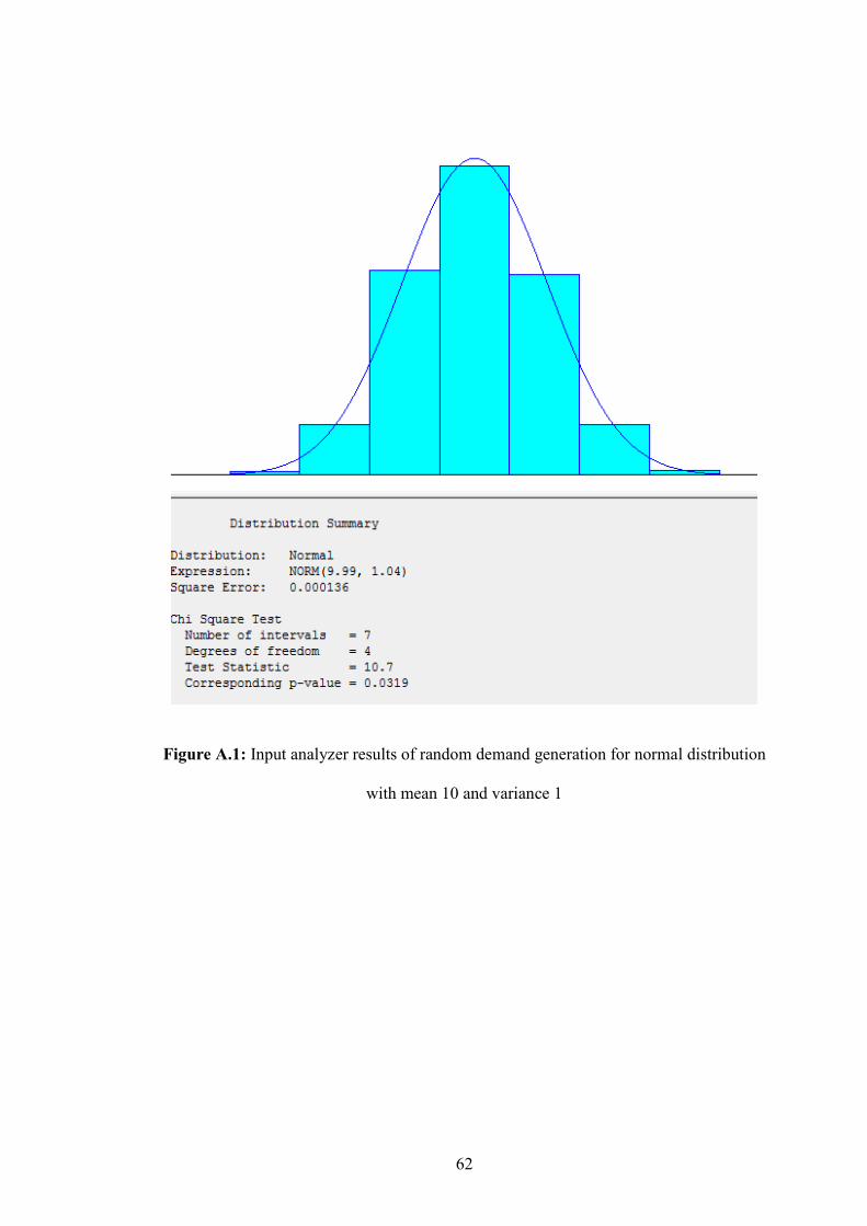
62

Figure A.1: Input analyzer results of random demand generation for normal distribution

with mean 10 and variance 1

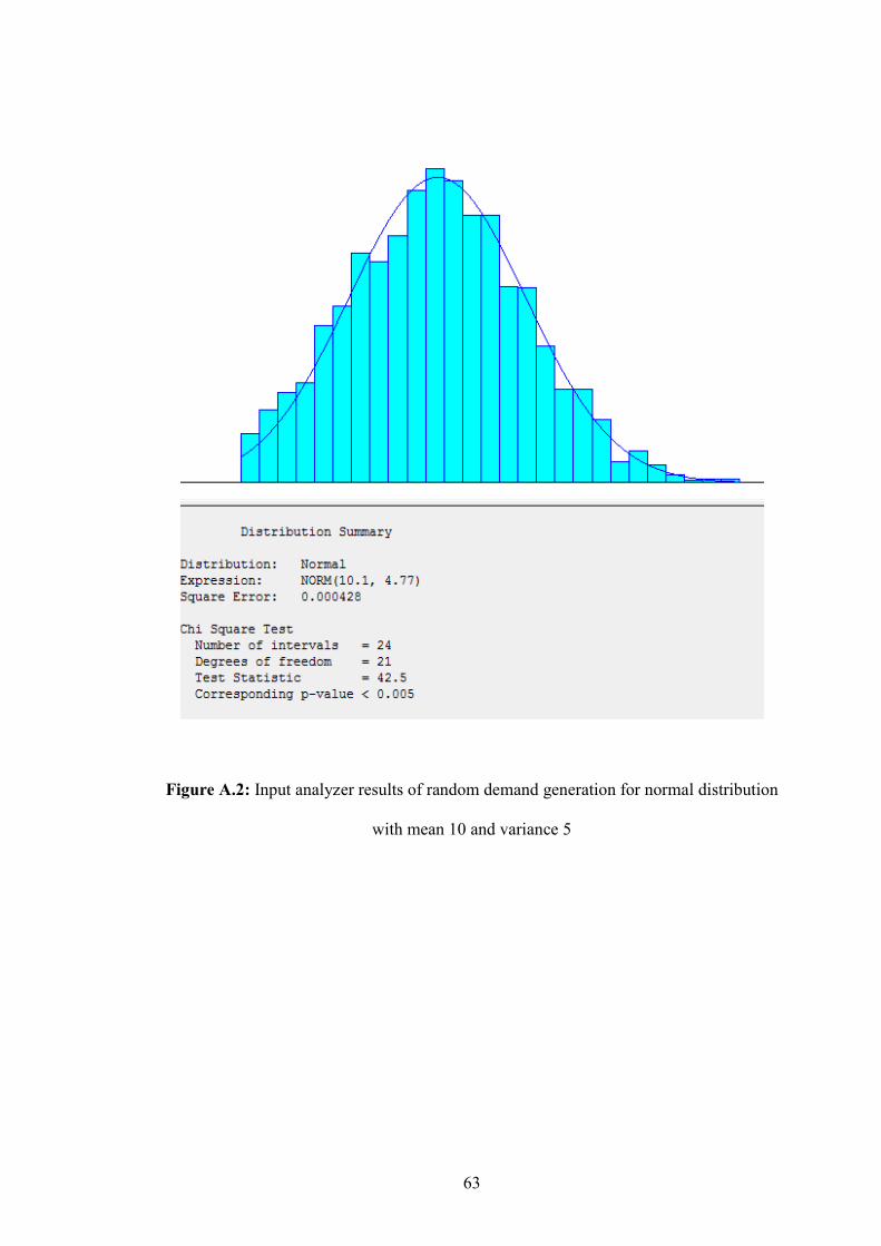
63

Figure A.2: Input analyzer results of random demand generation for normal distribution

with mean 10 and variance 5

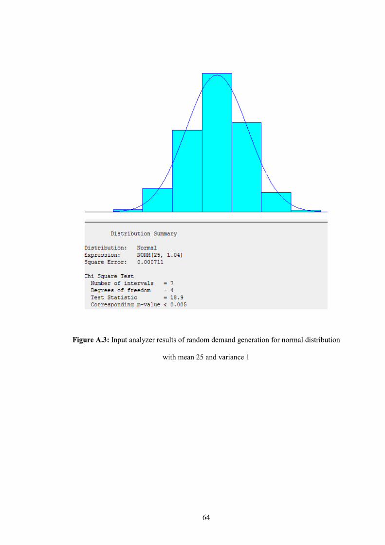
64

Figure A.3: Input analyzer results of random demand generation for normal distribution

with mean 25 and variance 1

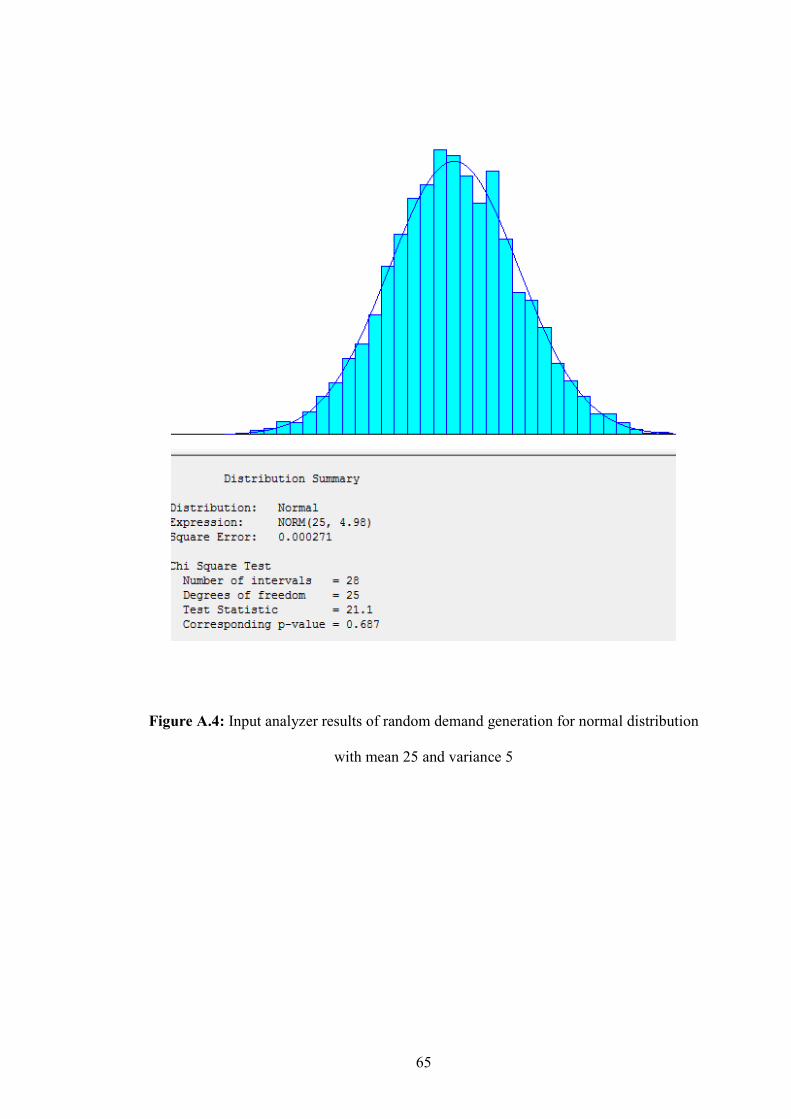
65

Figure A.4: Input analyzer results of random demand generation for normal distribution

with mean 25 and variance 5

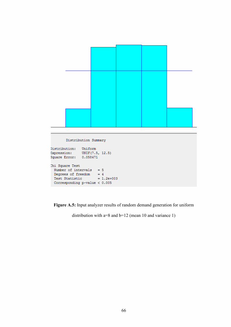
66

Figure A.5: Input analyzer results of random demand generation for uniform

distribution with a=8 and b=12 (mean 10 and variance 1)

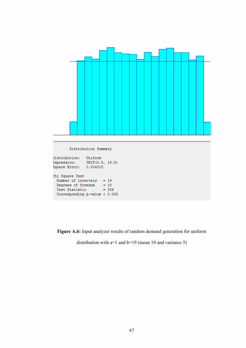
67

Figure A.6: Input analyzer results of random demand generation for uniform

distribution with a=1 and b=19 (mean 10 and variance 5)

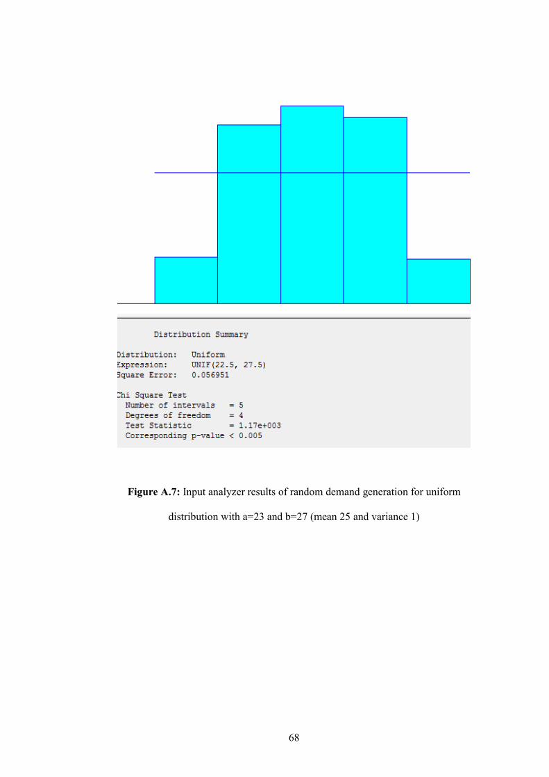
68

Figure A.7: Input analyzer results of random demand generation for uniform

distribution with a=23 and b=27 (mean 25 and variance 1)

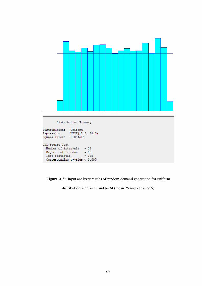
69

Figure A.8: Input analyzer results of random demand generation for uniform

distribution with a=16 and b=34 (mean 25 and variance 5)

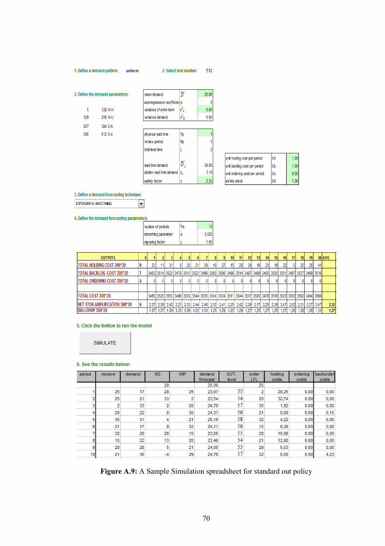
70

Figure A.9: A Sample Simulation spreadsheet for standard out policy

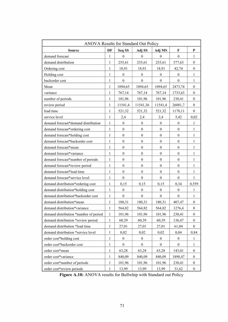
71

ANOVA Results for Standard Out Policy

Source DF Seq SS Adj SS Adj MS F P

demand forecast 1 0 0 0 0 1

demand distribution 1 255,61 255,61 255,61 577,63 0

Ordering cost 1 18,91 18,91 18,91 42,74 0

Holding cost 1 0 0 0 0 1

backorder cost 1 0 0 0 0 1

Mean 1 1094,65 1094,65 1094,65 2473,74 0

variance 1 767,14 767,14 767,14 1733,63 0

number of periods 1 101,96 101,96 101,96 230,41 0

review period 1 11541,4 11541,36 11541,4 26081,7 0

lead time 1 521,32 521,32 521,32 1178,11 0

service level 1 2,4 2,4 2,4 5,42 0,02

demand forecast*demand distribution 1 0 0 0 0 1

demand forecast*ordering cost 1 0 0 0 0 1

demand forecast*holding cost 1 0 0 0 0 1

demand forecast*backorder cost 1 0 0 0 0 1

demand forecast*mean 1 0 0 0 0 1

demand forecast*variance 1 0 0 0 0 1

demand forecast*number of periods 1 0 0 0 0 1

demand forecast*review period 1 0 0 0 0 1

demand forecast*lead time 1 0 0 0 0 1

demand forecast*service level 1 0 0 0 0 1

demand distribution*ordering cost 1 0,15 0,15 0,15 0,34 0,559

demand distribution*holding cost 1 0 0 0 0 1

demand distribution*backorder cost 1 0 0 0 0 1

demand distribution*mean 1 180,31 180,31 180,31 407,47 0

demand distribution*variance 1 564,82 564,82 564,82 1276,4 0

demand distribution *number of period 1 101,96 101,96 101,96 230,41 0

demand distribution *review period 1 60,39 60,39 60,39 136,47 0

demand distribution *lead time 1 27,01 27,01 27,01 61,04 0

demand distribution *service level 1 0,02 0,02 0,02 0,04 0,84

order cost*holding cost 1 0 0 0 0 1

order cost*backorder cost 1 0 0 0 0 1

order cost*mean 1 63,28 63,28 63,28 143,01 0

order cost*variance 1 840,09 840,09 840,09 1898,47 0

order cost*number of periods 1 101,96 101,96 101,96 230,41 0

order cost*review periods 1 13,99 13,99 13,99 31,62 0

Figure A.10: ANOVA results for Bullwhip with Standard out Policy

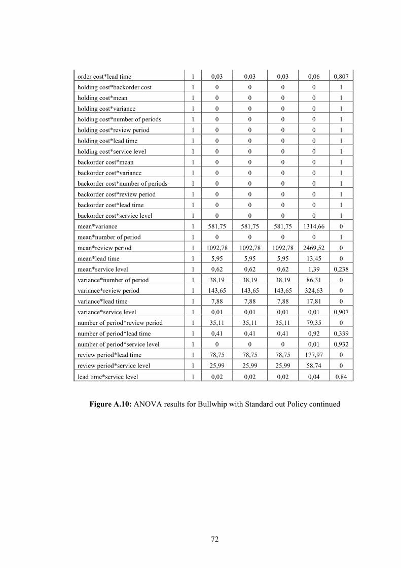
72

order cost*lead time 1 0,03 0,03 0,03 0,06 0,807

holding cost*backorder cost 1 0 0 0 0 1

holding cost*mean 1 0 0 0 0 1

holding cost*variance 1 0 0 0 0 1

holding cost*number of periods 1 0 0 0 0 1

holding cost*review period 1 0 0 0 0 1

holding cost*lead time 1 0 0 0 0 1

holding cost*service level 1 0 0 0 0 1

backorder cost*mean 1 0 0 0 0 1

backorder cost*variance 1 0 0 0 0 1

backorder cost*number of periods 1 0 0 0 0 1

backorder cost*review period 1 0 0 0 0 1

backorder cost*lead time 1 0 0 0 0 1

backorder cost*service level 1 0 0 0 0 1

mean*variance 1 581,75 581,75 581,75 1314,66 0

mean*number of period 1 0 0 0 0 1

mean*review period 1 1092,78 1092,78 1092,78 2469,52 0

mean*lead time 1 5,95 5,95 5,95 13,45 0

mean*service level 1 0,62 0,62 0,62 1,39 0,238

variance*number of period 1 38,19 38,19 38,19 86,31 0

variance*review period 1 143,65 143,65 143,65 324,63 0

variance*lead time 1 7,88 7,88 7,88 17,81 0

variance*service level 1 0,01 0,01 0,01 0,01 0,907

number of period*review period 1 35,11 35,11 35,11 79,35 0

number of period*lead time 1 0,41 0,41 0,41 0,92 0,339

number of period*service level 1 0 0 0 0,01 0,932

review period*lead time 1 78,75 78,75 78,75 177,97 0

review period*service level 1 25,99 25,99 25,99 58,74 0

lead time*service level 1 0,02 0,02 0,02 0,04 0,84

Figure A.10: ANOVA results for Bullwhip with Standard out Policy continued

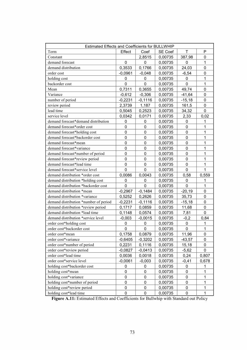
73

Estimated Effects and Coefficients for BULLWHIP

Term Effect Coef SE Coef T P

Constant 2,8515 0,00735 387,98 0

demand forecast 0 0 0,00735 0 1

demand distribution 0,3533 0,1766 0,00735 24,03 0

order cost -0,0961 -0,048 0,00735 -6,54 0

holding cost 0 0 0,00735 0 1

backorder cost 0 0 0,00735 0 1

Mean 0,7311 0,3655 0,00735 49,74 0

Variance -0,612 -0,306 0,00735 -41,64 0

number of period -0,2231 -0,1116 0,00735 -15,18 0

review period 2,3739 1,187 0,00735 161,5 0

lead time 0,5045 0,2523 0,00735 34,32 0

service level 0,0342 0,0171 0,00735 2,33 0,02

demand forecast*demand distribution 0 0 0,00735 0 1

demand forecast*order cost 0 0 0,00735 0 1

demand forecast*holding cost 0 0 0,00735 0 1

demand forecast*backorder cost 0 0 0,00735 0 1

demand forecast*mean 0 0 0,00735 0 1

demand forecast*variance 0 0 0,00735 0 1

demand forecast*number of period 0 0 0,00735 0 1

demand forecast*review period 0 0 0,00735 0 1

demand forecast*lead time 0 0 0,00735 0 1

demand forecast*service level 0 0 0,00735 0 1

demand distribution *order cost 0,0086 0,0043 0,00735 0,58 0,559

demand distribution *holding cost 0 0 0,00735 0 1

demand distribution *backorder cost 0 0 0,00735 0 1

demand distribution *mean -0,2967 -0,1484 0,00735 -20,19 0

demand distribution *variance 0,5252 0,2626 0,00735 35,73 0

demand distribution *number of period -0,2231 -0,1116 0,00735 -15,18 0

demand distribution *review period 0,1717 0,0859 0,00735 11,68 0

demand distribution *lead time 0,1148 0,0574 0,00735 7,81 0

demand distribution *service level -0,003 -0,0015 0,00735 -0,2 0,84

order cost*holding cost 0 0 0,00735 0 1

order cost*backorder cost 0 0 0,00735 0 1

order cost*mean 0,1758 0,0879 0,00735 11,96 0

order cost*variance -0,6405 -0,3202 0,00735 -43,57 0

order cost*number of period 0,2231 0,1116 0,00735 15,18 0

order cost*review period -0,0827 -0,0413 0,00735 -5,62 0

order cost*lead time 0,0036 0,0018 0,00735 0,24 0,807

order cost*service level -0,0061 -0,003 0,00735 -0,41 0,678

holding cost*backorder cost 0 0 0,00735 0 1

holding cost*mean 0 0 0,00735 0 1

holding cost*variance 0 0 0,00735 0 1

holding cost*number of period 0 0 0,00735 0 1

holding cost*review period 0 0 0,00735 0 1

holding cost*lead time 0 0 0,00735 0 1

Figure A.11: Estimated Effects and Coefficients for Bullwhip with Standard out Policy

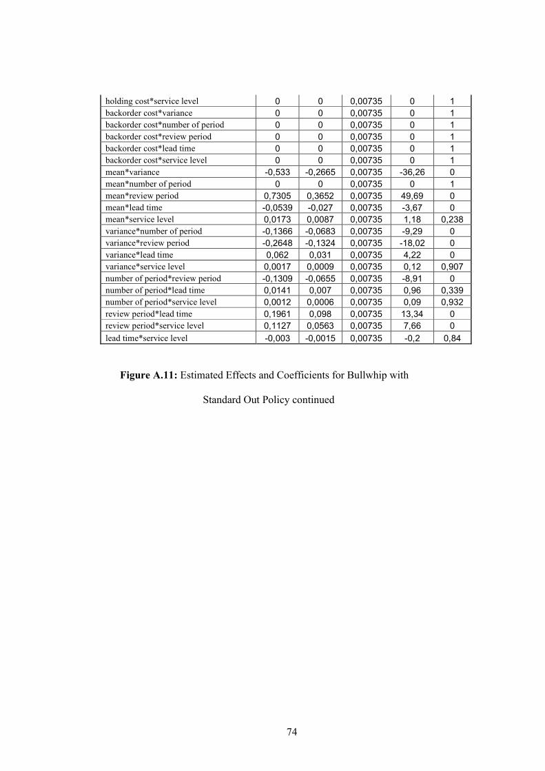
74

holding cost*service level 0 0 0,00735 0 1

backorder cost*variance 0 0 0,00735 0 1

backorder cost*number of period 0 0 0,00735 0 1

backorder cost*review period 0 0 0,00735 0 1

backorder cost*lead time 0 0 0,00735 0 1

backorder cost*service level 0 0 0,00735 0 1

mean*variance -0,533 -0,2665 0,00735 -36,26 0

mean*number of period 0 0 0,00735 0 1

mean*review period 0,7305 0,3652 0,00735 49,69 0

mean*lead time -0,0539 -0,027 0,00735 -3,67 0

mean*service level 0,0173 0,0087 0,00735 1,18 0,238

variance*number of period -0,1366 -0,0683 0,00735 -9,29 0

variance*review period -0,2648 -0,1324 0,00735 -18,02 0

variance*lead time 0,062 0,031 0,00735 4,22 0

variance*service level 0,0017 0,0009 0,00735 0,12 0,907

number of period*review period -0,1309 -0,0655 0,00735 -8,91 0

number of period*lead time 0,0141 0,007 0,00735 0,96 0,339

number of period*service level 0,0012 0,0006 0,00735 0,09 0,932

review period*lead time 0,1961 0,098 0,00735 13,34 0

review period*service level 0,1127 0,0563 0,00735 7,66 0

lead time*service level -0,003 -0,0015 0,00735 -0,2 0,84

Figure A.11: Estimated Effects and Coefficients for Bullwhip with

Standard Out Policy continued

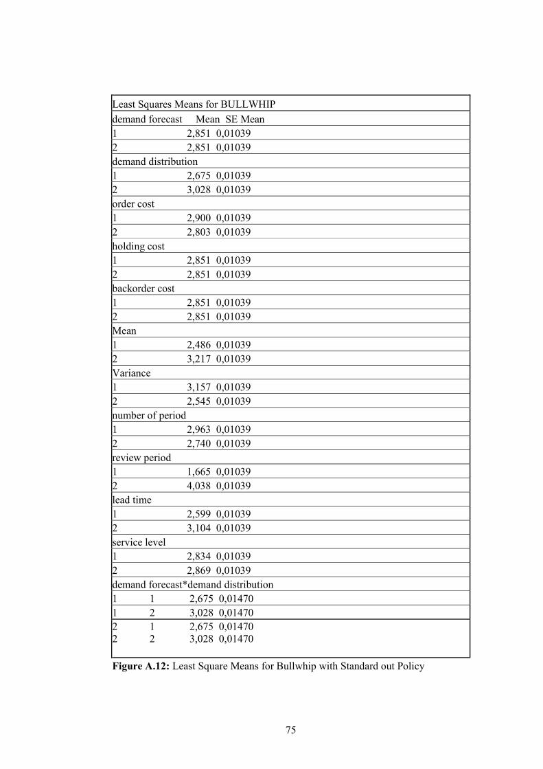
75

Least Squares Means for BULLWHIP

demand forecast Mean SE Mean

1 2,851 0,01039

2 2,851 0,01039

demand distribution

1 2,675 0,01039

2 3,028 0,01039

order cost

1 2,900 0,01039

2 2,803 0,01039

holding cost

1 2,851 0,01039

2 2,851 0,01039

backorder cost

1 2,851 0,01039

2 2,851 0,01039

Mean

1 2,486 0,01039

2 3,217 0,01039

Variance

1 3,157 0,01039

2 2,545 0,01039

number of period

1 2,963 0,01039

2 2,740 0,01039

review period

1 1,665 0,01039

2 4,038 0,01039

lead time

1 2,599 0,01039

2 3,104 0,01039

service level

1 2,834 0,01039

2 2,869 0,01039

demand forecast*demand distribution

1 1 2,675 0,01470

1 2 3,028 0,01470

2 1 2,675 0,01470

2 2 3,028 0,01470

Figure A.12: Least Square Means for Bullwhip with Standard out Policy

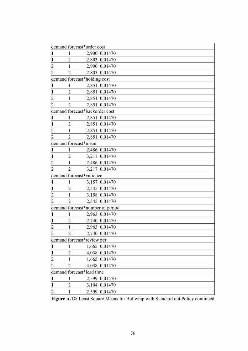
76

demand forecast*order cost

1 1 2,900 0,01470

1 2 2,803 0,01470

2 1 2,900 0,01470

2 2 2,803 0,01470

demand forecast*holding cost

1 1 2,851 0,01470

1 2 2,851 0,01470

2 1 2,851 0,01470

2 2 2,851 0,01470

demand forecast*backorder cost

1 1 2,851 0,01470

1 2 2,851 0,01470

2 1 2,851 0,01470

2 2 2,851 0,01470

demand forecast*mean

1 1 2,486 0,01470

1 2 3,217 0,01470

2 1 2,486 0,01470

2 2 3,217 0,01470

demand forecast*variance

1 1 3,157 0,01470

1 2 2,545 0,01470

2 1 3,158 0,01470

2 2 2,545 0,01470

demand forecast*number of period

1 1 2,963 0,01470

1 2 2,740 0,01470

2 1 2,963 0,01470

2 2 2,740 0,01470

demand forecast*review per

1 1 1,665 0,01470

1 2 4,038 0,01470

2 1 1,665 0,01470

2 2 4,038 0,01470

demand forecast*lead time

1 1 2,599 0,01470

1 2 3,104 0,01470

2 1 2,599 0,01470

Figure A.12: Least Square Means for Bullwhip with Standard out Policy continued

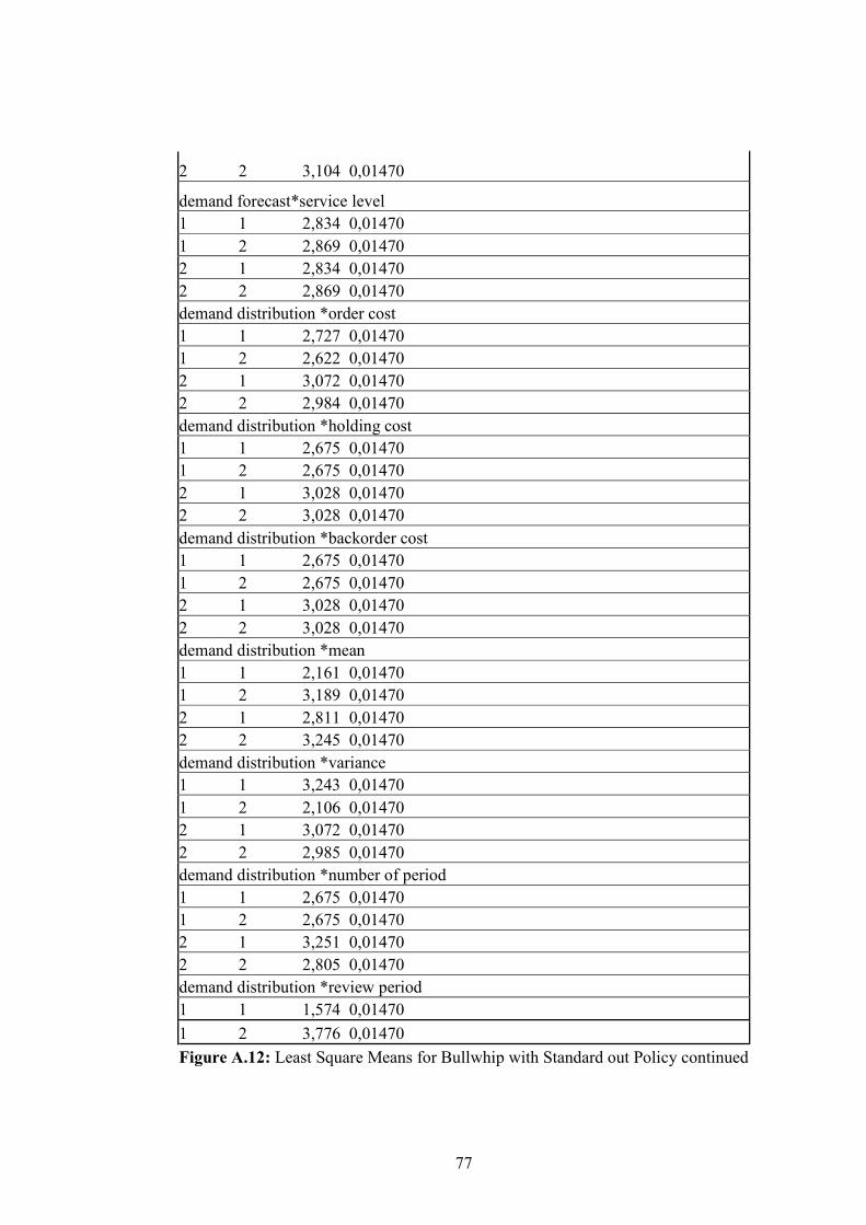
77

2 2 3,104 0,01470

demand forecast*service level

1 1 2,834 0,01470

1 2 2,869 0,01470

2 1 2,834 0,01470

2 2 2,869 0,01470

demand distribution *order cost

1 1 2,727 0,01470

1 2 2,622 0,01470

2 1 3,072 0,01470

2 2 2,984 0,01470

demand distribution *holding cost

1 1 2,675 0,01470

1 2 2,675 0,01470

2 1 3,028 0,01470

2 2 3,028 0,01470

demand distribution *backorder cost

1 1 2,675 0,01470

1 2 2,675 0,01470

2 1 3,028 0,01470

2 2 3,028 0,01470

demand distribution *mean

1 1 2,161 0,01470

1 2 3,189 0,01470

2 1 2,811 0,01470

2 2 3,245 0,01470

demand distribution *variance

1 1 3,243 0,01470

1 2 2,106 0,01470

2 1 3,072 0,01470

2 2 2,985 0,01470

demand distribution *number of period

1 1 2,675 0,01470

1 2 2,675 0,01470

2 1 3,251 0,01470

2 2 2,805 0,01470

demand distribution *review period

1 1 1,574 0,01470

1 2 3,776 0,01470

Figure A.12: Least Square Means for Bullwhip with Standard out Policy continued

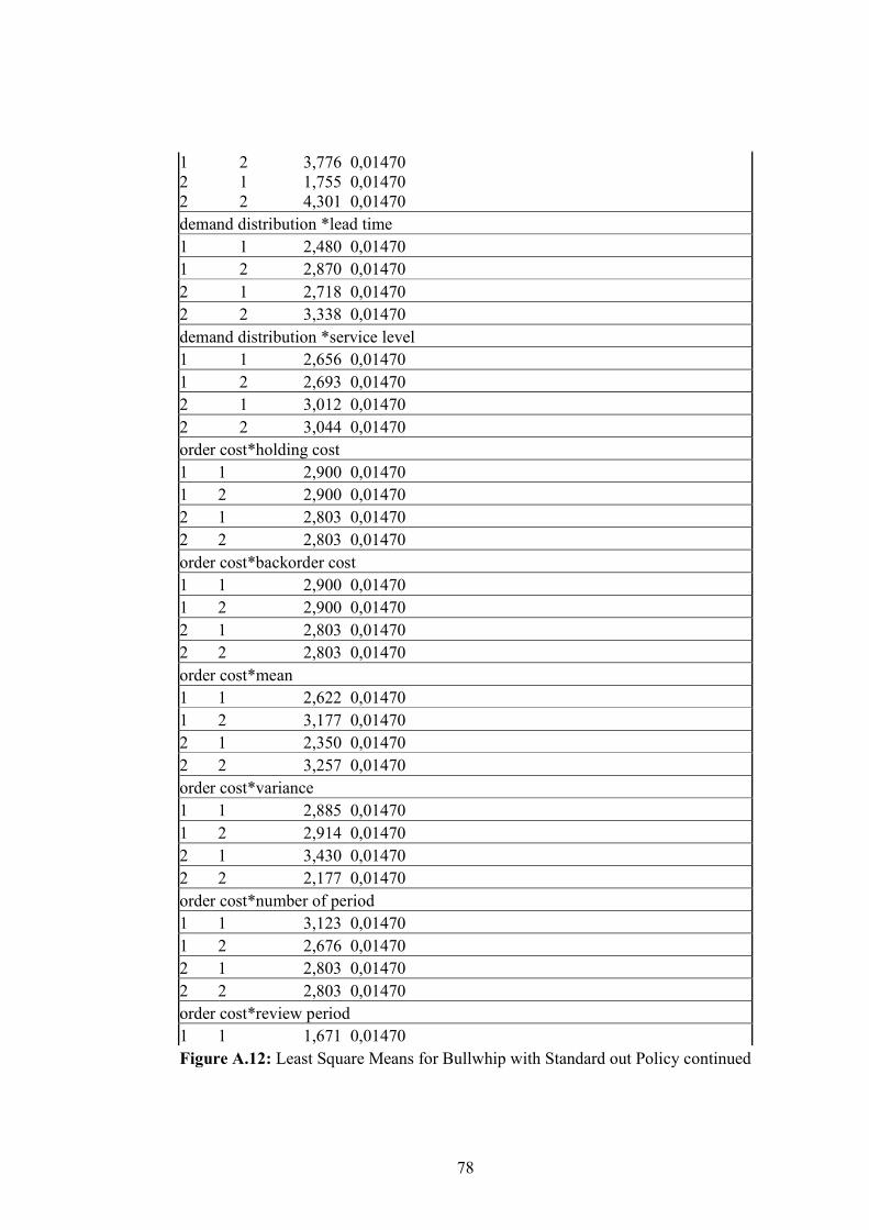
78

1 2 3,776 0,01470

2 1 1,755 0,01470

2 2 4,301 0,01470

demand distribution *lead time

1 1 2,480 0,01470

1 2 2,870 0,01470

2 1 2,718 0,01470

2 2 3,338 0,01470

demand distribution *service level

1 1 2,656 0,01470

1 2 2,693 0,01470

2 1 3,012 0,01470

2 2 3,044 0,01470

order cost*holding cost

1 1 2,900 0,01470

1 2 2,900 0,01470

2 1 2,803 0,01470

2 2 2,803 0,01470

order cost*backorder cost

1 1 2,900 0,01470

1 2 2,900 0,01470

2 1 2,803 0,01470

2 2 2,803 0,01470

order cost*mean

1 1 2,622 0,01470

1 2 3,177 0,01470

2 1 2,350 0,01470

2 2 3,257 0,01470

order cost*variance

1 1 2,885 0,01470

1 2 2,914 0,01470

2 1 3,430 0,01470

2 2 2,177 0,01470

order cost*number of period

1 1 3,123 0,01470

1 2 2,676 0,01470

2 1 2,803 0,01470

2 2 2,803 0,01470

order cost*review period

1 1 1,671 0,01470

Figure A.12: Least Square Means for Bullwhip with Standard out Policy continued

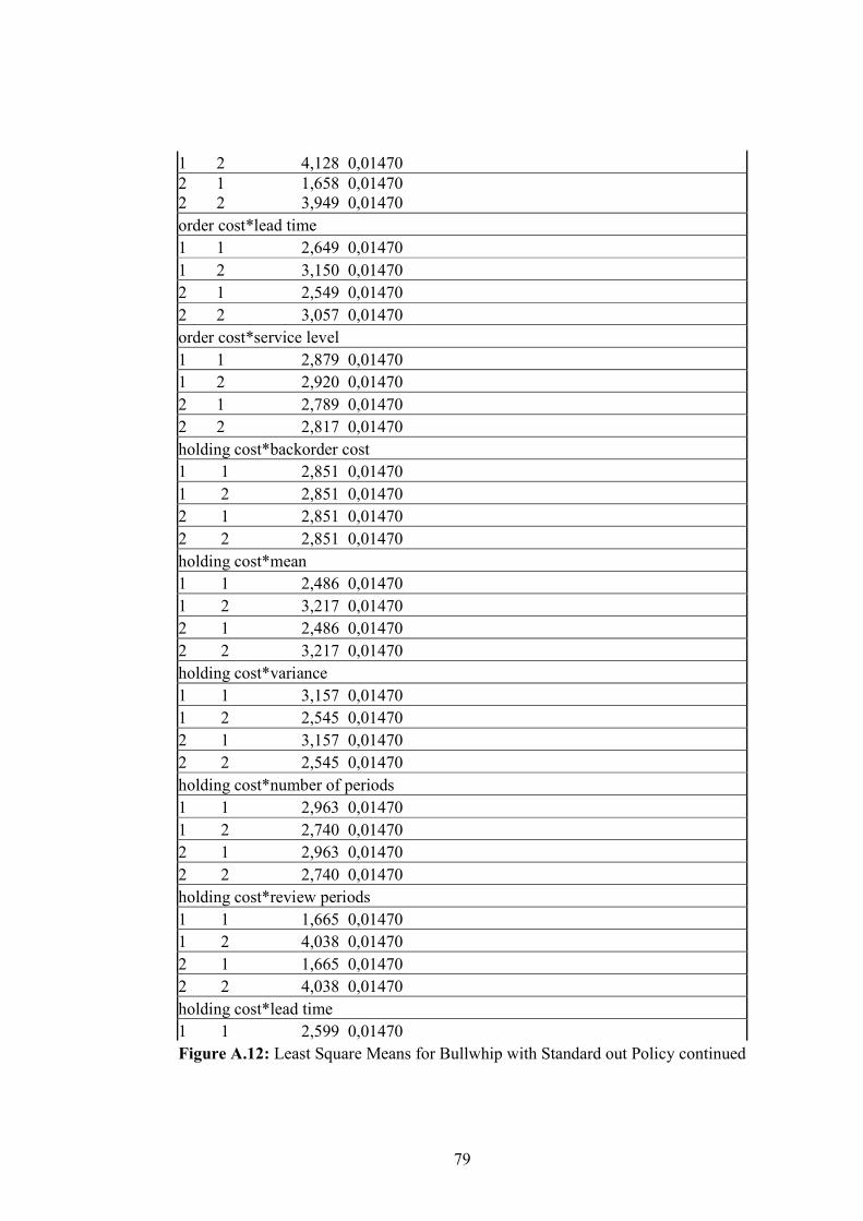
79

1 2 4,128 0,01470

2 1 1,658 0,01470

2 2 3,949 0,01470

order cost*lead time

1 1 2,649 0,01470

1 2 3,150 0,01470

2 1 2,549 0,01470

2 2 3,057 0,01470

order cost*service level

1 1 2,879 0,01470

1 2 2,920 0,01470

2 1 2,789 0,01470

2 2 2,817 0,01470

holding cost*backorder cost

1 1 2,851 0,01470

1 2 2,851 0,01470

2 1 2,851 0,01470

2 2 2,851 0,01470

holding cost*mean

1 1 2,486 0,01470

1 2 3,217 0,01470

2 1 2,486 0,01470

2 2 3,217 0,01470

holding cost*variance

1 1 3,157 0,01470

1 2 2,545 0,01470

2 1 3,157 0,01470

2 2 2,545 0,01470

holding cost*number of periods

1 1 2,963 0,01470

1 2 2,740 0,01470

2 1 2,963 0,01470

2 2 2,740 0,01470

holding cost*review periods

1 1 1,665 0,01470

1 2 4,038 0,01470

2 1 1,665 0,01470

2 2 4,038 0,01470

holding cost*lead time

1 1 2,599 0,01470

Figure A.12: Least Square Means for Bullwhip with Standard out Policy continued

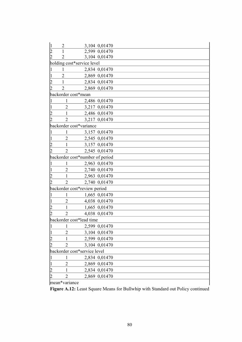
80

1 2 3,104 0,01470

2 1 2,599 0,01470

2 2 3,104 0,01470

holding cost*service level

1 1 2,834 0,01470

1 2 2,869 0,01470

2 1 2,834 0,01470

2 2 2,869 0,01470

backorder cost*mean

1 1 2,486 0,01470

1 2 3,217 0,01470

2 1 2,486 0,01470

2 2 3,217 0,01470

backorder cost*variance

1 1 3,157 0,01470

1 2 2,545 0,01470

2 1 3,157 0,01470

2 2 2,545 0,01470

backorder cost*number of period

1 1 2,963 0,01470

1 2 2,740 0,01470

2 1 2,963 0,01470

2 2 2,740 0,01470

backorder cost*review period

1 1 1,665 0,01470

1 2 4,038 0,01470

2 1 1,665 0,01470

2 2 4,038 0,01470

backorder cost*lead time

1 1 2,599 0,01470

1 2 3,104 0,01470

2 1 2,599 0,01470

2 2 3,104 0,01470

backorder cost*service level

1 1 2,834 0,01470

1 2 2,869 0,01470

2 1 2,834 0,01470

2 2 2,869 0,01470

mean*variance

Figure A.12: Least Square Means for Bullwhip with Standard out Policy continued

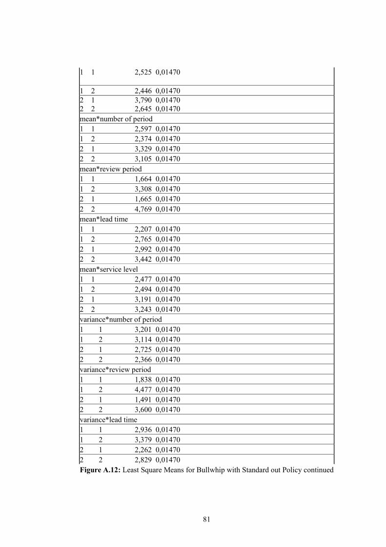
81

1 1 2,525 0,01470

1 2 2,446 0,01470

2 1 3,790 0,01470

2 2 2,645 0,01470

mean*number of period

1 1 2,597 0,01470

1 2 2,374 0,01470

2 1 3,329 0,01470

2 2 3,105 0,01470

mean*review period

1 1 1,664 0,01470

1 2 3,308 0,01470

2 1 1,665 0,01470

2 2 4,769 0,01470

mean*lead time

1 1 2,207 0,01470

1 2 2,765 0,01470

2 1 2,992 0,01470

2 2 3,442 0,01470

mean*service level

1 1 2,477 0,01470

1 2 2,494 0,01470

2 1 3,191 0,01470

2 2 3,243 0,01470

variance*number of period

1 1 3,201 0,01470

1 2 3,114 0,01470

2 1 2,725 0,01470

2 2 2,366 0,01470

variance*review period

1 1 1,838 0,01470

1 2 4,477 0,01470

2 1 1,491 0,01470

2 2 3,600 0,01470

variance*lead time

1 1 2,936 0,01470

1 2 3,379 0,01470

2 1 2,262 0,01470

2 2 2,829 0,01470

Figure A.12: Least Square Means for Bullwhip with Standard out Policy continued

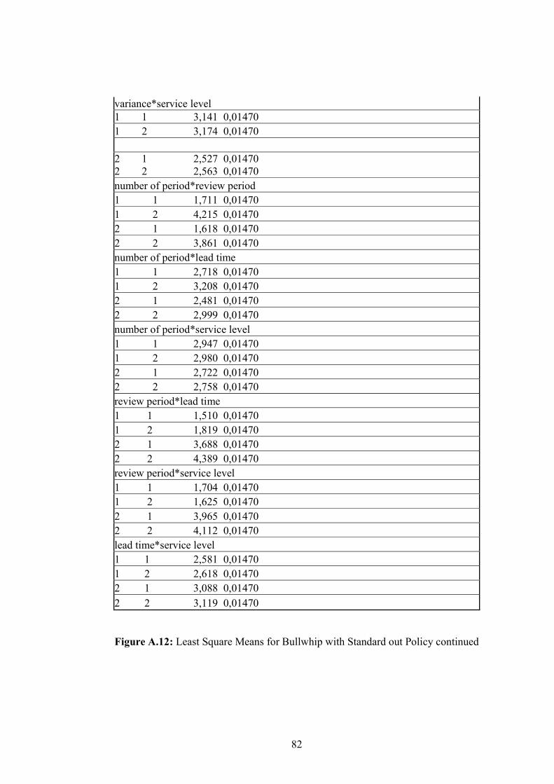
82

variance*service level

1 1 3,141 0,01470

1 2 3,174 0,01470

2 1 2,527 0,01470

2 2 2,563 0,01470

number of period*review period

1 1 1,711 0,01470

1 2 4,215 0,01470

2 1 1,618 0,01470

2 2 3,861 0,01470

number of period*lead time

1 1 2,718 0,01470

1 2 3,208 0,01470

2 1 2,481 0,01470

2 2 2,999 0,01470

number of period*service level

1 1 2,947 0,01470

1 2 2,980 0,01470

2 1 2,722 0,01470

2 2 2,758 0,01470

review period*lead time

1 1 1,510 0,01470

1 2 1,819 0,01470

2 1 3,688 0,01470

2 2 4,389 0,01470

review period*service level

1 1 1,704 0,01470

1 2 1,625 0,01470

2 1 3,965 0,01470

2 2 4,112 0,01470

lead time*service level

1 1 2,581 0,01470

1 2 2,618 0,01470

2 1 3,088 0,01470

2 2 3,119 0,01470

Figure A.12: Least Square Means for Bullwhip with Standard out Policy continued

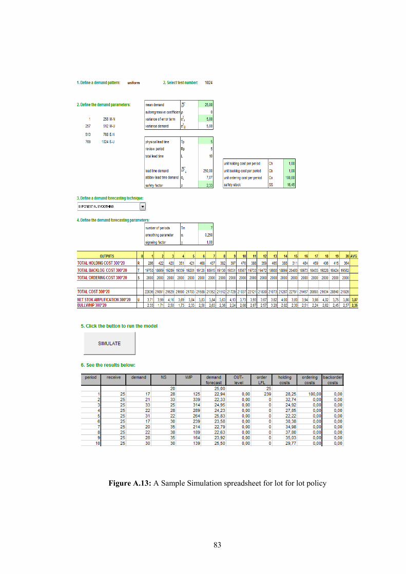
83

Figure A.13: A Sample Simulation spreadsheet for lot for lot policy

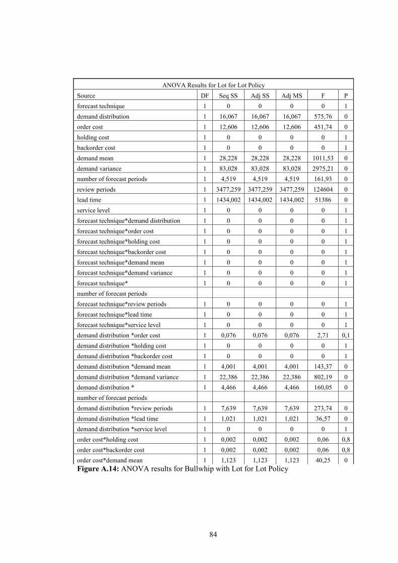
84

ANOVA Results for Lot for Lot Policy

Source DF Seq SS Adj SS Adj MS F P

forecast technique 1 0 0 0 0 1

demand distribution 1 16,067 16,067 16,067 575,76 0

order cost 1 12,606 12,606 12,606 451,74 0

holding cost 1 0 0 0 0 1

backorder cost 1 0 0 0 0 1

demand mean 1 28,228 28,228 28,228 1011,53 0

demand variance 1 83,028 83,028 83,028 2975,21 0

number of forecast periods 1 4,519 4,519 4,519 161,93 0

review periods 1 3477,259 3477,259 3477,259 124604 0

lead time 1 1434,002 1434,002 1434,002 51386 0

service level 1 0 0 0 0 1

forecast technique*demand distribution 1 0 0 0 0 1

forecast technique*order cost 1 0 0 0 0 1

forecast technique*holding cost 1 0 0 0 0 1

forecast technique*backorder cost 1 0 0 0 0 1

forecast technique*demand mean 1 0 0 0 0 1

forecast technique*demand variance 1 0 0 0 0 1

forecast technique* 1 0 0 0 0 1

number of forecast periods

forecast technique*review periods 1 0 0 0 0 1

forecast technique*lead time 1 0 0 0 0 1

forecast technique*service level 1 0 0 0 0 1

demand distribution *order cost 1 0,076 0,076 0,076 2,71 0,1

demand distribution *holding cost 1 0 0 0 0 1

demand distribution *backorder cost 1 0 0 0 0 1

demand distribution *demand mean 1 4,001 4,001 4,001 143,37 0

demand distribution *demand variance 1 22,386 22,386 22,386 802,19 0

demand distribution * 1 4,466 4,466 4,466 160,05 0

number of forecast periods

demand distribution *review periods 1 7,639 7,639 7,639 273,74 0

demand distribution *lead time 1 1,021 1,021 1,021 36,57 0

demand distribution *service level 1 0 0 0 0 1

order cost*holding cost 1 0,002 0,002 0,002 0,06 0,8

order cost*backorder cost 1 0,002 0,002 0,002 0,06 0,8

order cost*demand mean 1 1,123 1,123 1,123 40,25 0

Figure A.14: ANOVA results for Bullwhip with Lot for Lot Policy

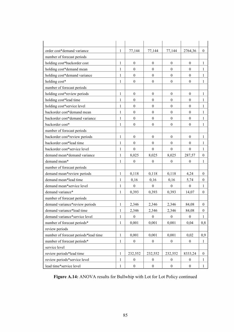
85

order cost*demand variance 1 77,144 77,144 77,144 2764,36 0

number of forecast periods

holding cost*backorder cost 1 0 0 0 0 1

holding cost*demand mean 1 0 0 0 0 1

holding cost*demand variance 1 0 0 0 0 1

holding cost* 1 0 0 0 0 1

number of forecast periods

holding cost*review periods 1 0 0 0 0 1

holding cost*lead time 1 0 0 0 0 1

holding cost*service level 1 0 0 0 0 1

backorder cost*demand mean 1 0 0 0 0 1

backorder cost*demand variance 1 0 0 0 0 1

backorder cost* 1 0 0 0 0 1

number of forecast periods

backorder cost*review periods 1 0 0 0 0 1

backorder cost*lead time 1 0 0 0 0 1

backorder cost*service level 1 0 0 0 0 1

demand mean*demand variance 1 8,025 8,025 8,025 287,57 0

demand mean* 1 0 0 0 0 1

number of forecast periods

demand mean*review periods 1 0,118 0,118 0,118 4,24 0

demand mean*lead time 1 0,16 0,16 0,16 5,74 0

demand mean*service level 1 0 0 0 0 1

demand variance* 1 0,393 0,393 0,393 14,07 0

number of forecast periods

demand variance*review periods 1 2,346 2,346 2,346 84,08 0

demand variance*lead time 1 2,346 2,346 2,346 84,08 0

demand variance*service level 1 0 0 0 0 1

number of forecast periods* 1 0,001 0,001 0,001 0,04 0,8

review periods

number of forecast periods*lead time 1 0,001 0,001 0,001 0,02 0,9

number of forecast periods* 1 0 0 0 0 1

service level

review periods*lead time 1 232,552 232,552 232,552 8333,24 0

review periods*service level 1 0 0 0 0 1

lead time*service level 1 0 0 0 0 1

Figure A.14: ANOVA results for Bullwhip with Lot for Lot Policy continued

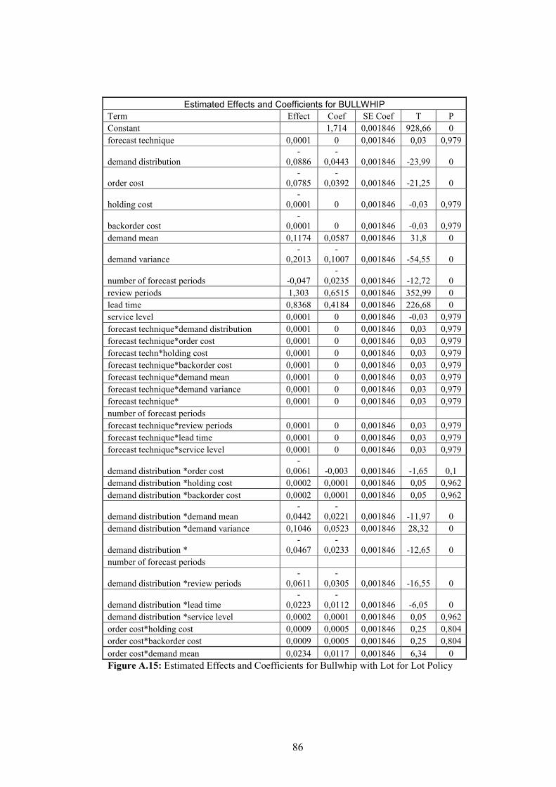
86

Estimated Effects and Coefficients for BULLWHIP

Term Effect Coef SE Coef T P

Constant 1,714 0,001846 928,66 0

forecast technique 0,0001 0 0,001846 0,03 0,979

demand distribution

-

0,0886

-

0,0443 0,001846 -23,99 0

order cost

-

0,0785

-

0,0392 0,001846 -21,25 0

holding cost

-

0,0001 0 0,001846 -0,03 0,979

backorder cost

-

0,0001 0 0,001846 -0,03 0,979

demand mean 0,1174 0,0587 0,001846 31,8 0

demand variance

-

0,2013

-

0,1007 0,001846 -54,55 0

number of forecast periods -0,047

-

0,0235 0,001846 -12,72 0

review periods 1,303 0,6515 0,001846 352,99 0

lead time 0,8368 0,4184 0,001846 226,68 0

service level 0,0001 0 0,001846 -0,03 0,979

forecast technique*demand distribution 0,0001 0 0,001846 0,03 0,979

forecast technique*order cost 0,0001 0 0,001846 0,03 0,979

forecast techn*holding cost 0,0001 0 0,001846 0,03 0,979

forecast technique*backorder cost 0,0001 0 0,001846 0,03 0,979

forecast technique*demand mean 0,0001 0 0,001846 0,03 0,979

forecast technique*demand variance 0,0001 0 0,001846 0,03 0,979

forecast technique* 0,0001 0 0,001846 0,03 0,979

number of forecast periods

forecast technique*review periods 0,0001 0 0,001846 0,03 0,979

forecast technique*lead time 0,0001 0 0,001846 0,03 0,979

forecast technique*service level 0,0001 0 0,001846 0,03 0,979

demand distribution *order cost

-

0,0061 -0,003 0,001846 -1,65 0,1

demand distribution *holding cost 0,0002 0,0001 0,001846 0,05 0,962

demand distribution *backorder cost 0,0002 0,0001 0,001846 0,05 0,962

demand distribution *demand mean

-

0,0442

-

0,0221 0,001846 -11,97 0

demand distribution *demand variance 0,1046 0,0523 0,001846 28,32 0

demand distribution *

-

0,0467

-

0,0233 0,001846 -12,65 0

number of forecast periods

demand distribution *review periods

-

0,0611

-

0,0305 0,001846 -16,55 0

demand distribution *lead time

-

0,0223

-

0,0112 0,001846 -6,05 0

demand distribution *service level 0,0002 0,0001 0,001846 0,05 0,962

order cost*holding cost 0,0009 0,0005 0,001846 0,25 0,804

order cost*backorder cost 0,0009 0,0005 0,001846 0,25 0,804

order cost*demand mean 0,0234 0,0117 0,001846 6,34 0

Figure A.15: Estimated Effects and Coefficients for Bullwhip with Lot for Lot Policy

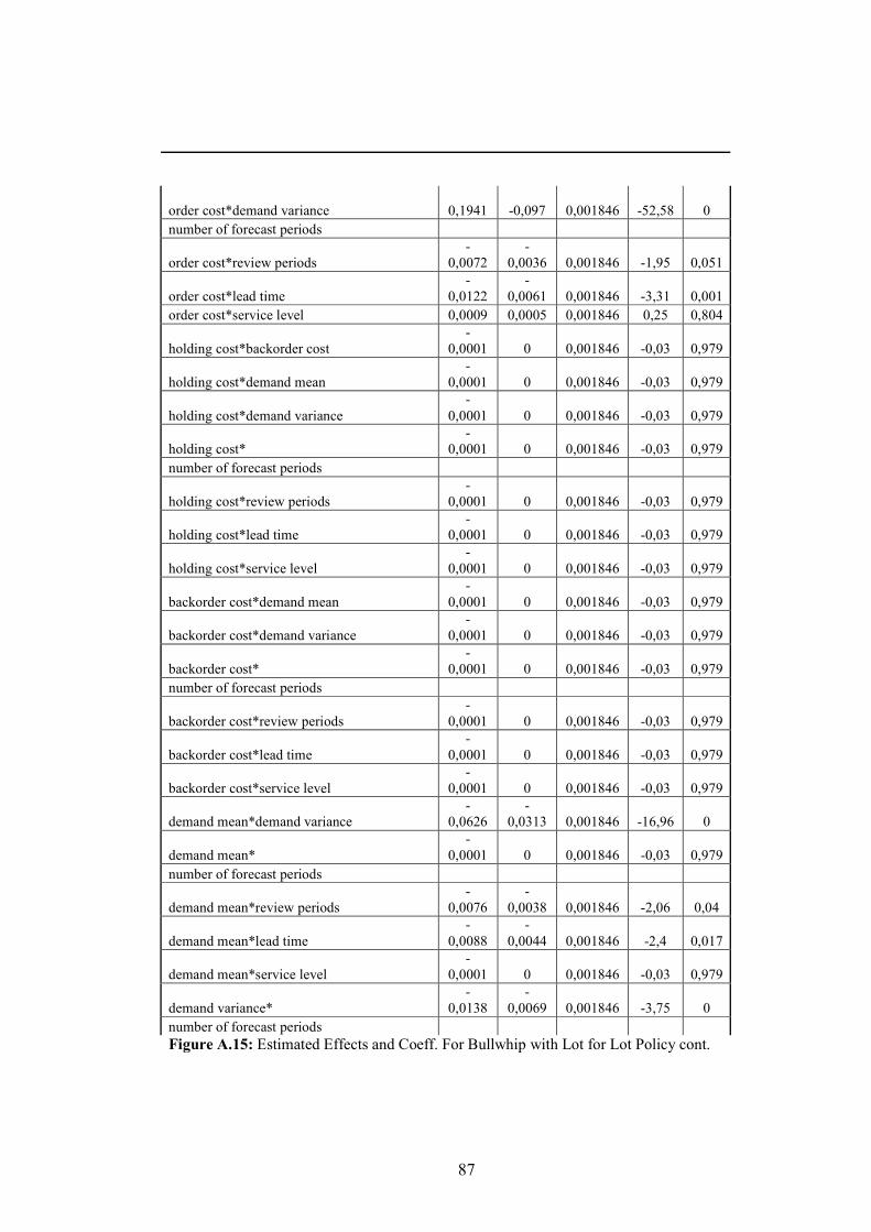
87

order cost*demand variance 0,1941 -0,097 0,001846 -52,58

0

number of forecast periods

order cost*review periods

-

0,0072

-

0,0036 0,001846 -1,95 0,051

order cost*lead time

-

0,0122

-

0,0061 0,001846 -3,31 0,001

order cost*service level 0,0009 0,0005 0,001846 0,25 0,804

holding cost*backorder cost

-

0,0001 0 0,001846 -0,03 0,979

holding cost*demand mean

-

0,0001 0 0,001846 -0,03 0,979

holding cost*demand variance

-

0,0001 0 0,001846 -0,03 0,979

holding cost*

-

0,0001 0 0,001846 -0,03 0,979

number of forecast periods

holding cost*review periods

-

0,0001 0 0,001846 -0,03 0,979

holding cost*lead time

-

0,0001 0 0,001846 -0,03 0,979

holding cost*service level

-

0,0001 0 0,001846 -0,03 0,979

backorder cost*demand mean

-

0,0001 0 0,001846 -0,03 0,979

backorder cost*demand variance

-

0,0001 0 0,001846 -0,03 0,979

backorder cost*

-

0,0001 0 0,001846 -0,03 0,979

number of forecast periods

backorder cost*review periods

-

0,0001 0 0,001846 -0,03 0,979

backorder cost*lead time

-

0,0001 0 0,001846 -0,03 0,979

backorder cost*service level

-

0,0001 0 0,001846 -0,03 0,979

demand mean*demand variance

-

0,0626

-

0,0313 0,001846 -16,96 0

demand mean*

-

0,0001 0 0,001846 -0,03 0,979

number of forecast periods

demand mean*review periods

-

0,0076

-

0,0038 0,001846 -2,06 0,04

demand mean*lead time

-

0,0088

-

0,0044 0,001846 -2,4 0,017

demand mean*service level

-

0,0001 0 0,001846 -0,03 0,979

demand variance*

-

0,0138

-

0,0069 0,001846 -3,75 0

number of forecast periods

Figure A.15: Estimated Effects and Coeff. For Bullwhip with Lot for Lot Policy cont.

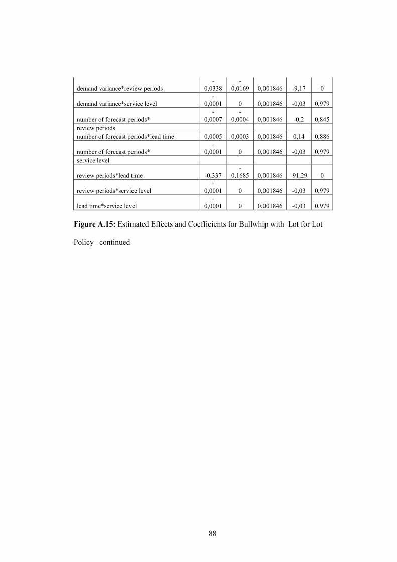
88

demand variance*review periods

-

0,0338

-

0,0169 0,001846 -9,17 0

demand variance*service level

-

0,0001 0 0,001846 -0,03 0,979

number of forecast periods*

-

0,0007

-

0,0004 0,001846 -0,2 0,845

review periods

number of forecast periods*lead time 0,0005 0,0003 0,001846 0,14 0,886

number of forecast periods*

-

0,0001 0 0,001846 -0,03 0,979

service level

review periods*lead time -0,337

-

0,1685 0,001846 -91,29 0

review periods*service level

-

0,0001 0 0,001846 -0,03 0,979

lead time*service level

-

0,0001 0 0,001846 -0,03 0,979

Figure A.15: Estimated Effects and Coefficients for Bullwhip with Lot for Lot

Policy continued

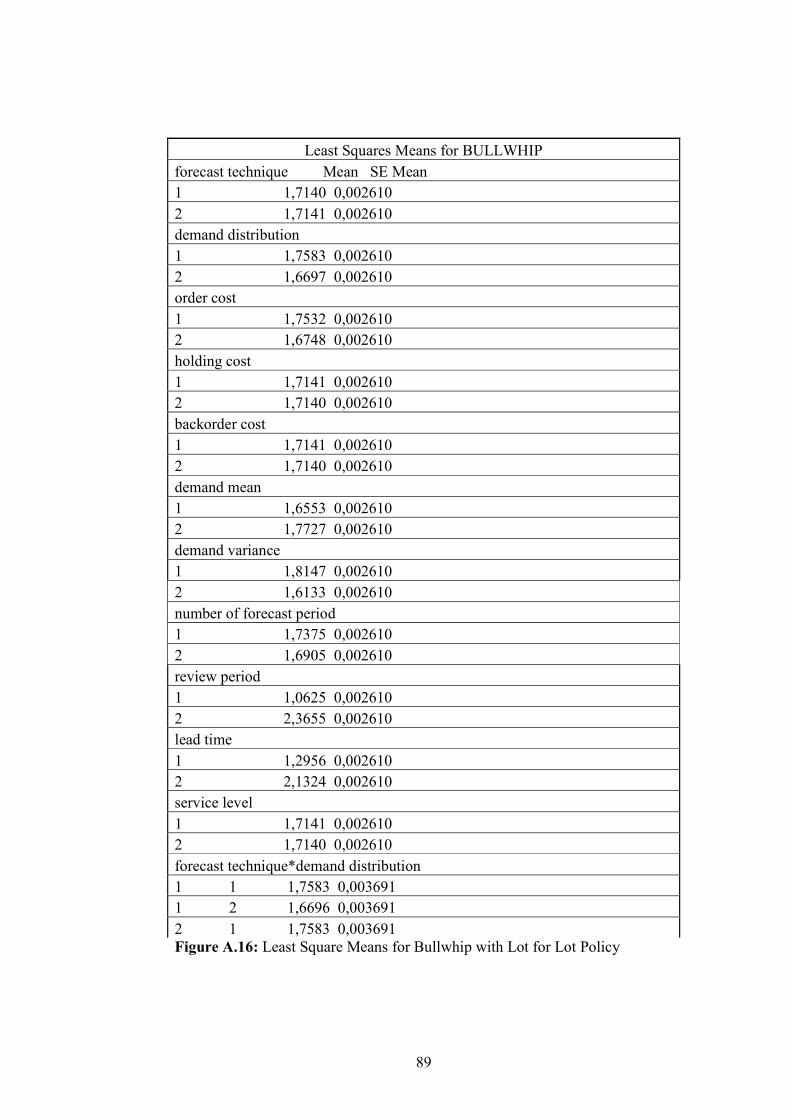
89

Least Squares Means for BULLWHIP

forecast technique Mean SE Mean

1 1,7140 0,002610

2 1,7141 0,002610

demand distribution

1 1,7583 0,002610

2 1,6697 0,002610

order cost

1 1,7532 0,002610

2 1,6748 0,002610

holding cost

1 1,7141 0,002610

2 1,7140 0,002610

backorder cost

1 1,7141 0,002610

2 1,7140 0,002610

demand mean

1 1,6553 0,002610

2 1,7727 0,002610

demand variance

1 1,8147 0,002610

2 1,6133 0,002610

number of forecast period

1 1,7375 0,002610

2 1,6905 0,002610

review period

1 1,0625 0,002610

2 2,3655 0,002610

lead time

1 1,2956 0,002610

2 2,1324 0,002610

service level

1 1,7141 0,002610

2 1,7140 0,002610

forecast technique*demand distribution

1 1 1,7583 0,003691

1 2 1,6696 0,003691

2 1 1,7583 0,003691

Figure A.16: Least Square Means for Bullwhip with Lot for Lot Policy

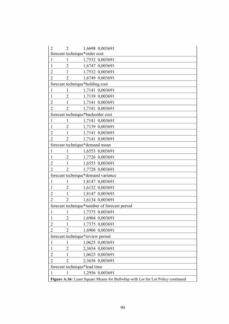
90

2 2 1,6698 0,003691

forecast technique*order cost

1 1 1,7532 0,003691

1 2 1,6747 0,003691

2 1 1,7532 0,003691

2 2 1,6749 0,003691

forecast technique*holding cost

1 1 1,7141 0,003691

1 2 1,7139 0,003691

2 1 1,7141 0,003691

2 2 1,7141 0,003691

forecast technique*backorder cost

1 1 1,7141 0,003691

1 2 1,7139 0,003691

2 1 1,7141 0,003691

2 2 1,7141 0,003691

forecast technique*demand mean

1 1 1,6553 0,003691

1 2 1,7726 0,003691

2 1 1,6553 0,003691

2 2 1,7728 0,003691

forecast technique*demand variance

1 1 1,8147 0,003691

1 2 1,6132 0,003691

2 1 1,8147 0,003691

2 2 1,6134 0,003691

forecast technique*number of forecast period

1 1 1,7375 0,003691

1 2 1,6904 0,003691

2 1 1,7375 0,003691

2 2 1,6906 0,003691

forecast technique*review period

1 1 1,0625 0,003691

1 2 2,3654 0,003691

2 1 1,0625 0,003691

2 2 2,3656 0,003691

forecast technique*lead time

1 1 1,2956 0,003691

Figure A.16: Least Square Means for Bullwhip with Lot for Lot Policy continued

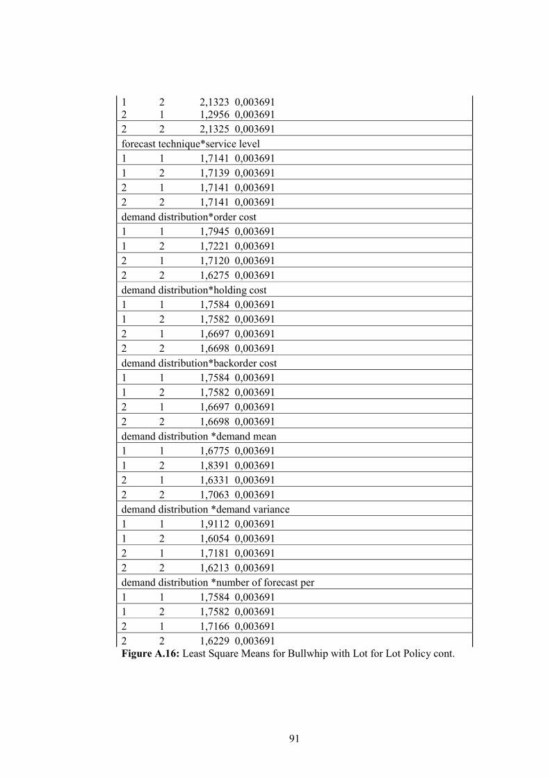
91

1 2 2,1323 0,003691

2 1 1,2956 0,003691

2 2 2,1325 0,003691

forecast technique*service level

1 1 1,7141 0,003691

1 2 1,7139 0,003691

2 1 1,7141 0,003691

2 2 1,7141 0,003691

demand distribution*order cost

1 1 1,7945 0,003691

1 2 1,7221 0,003691

2 1 1,7120 0,003691

2 2 1,6275 0,003691

demand distribution*holding cost

1 1 1,7584 0,003691

1 2 1,7582 0,003691

2 1 1,6697 0,003691

2 2 1,6698 0,003691

demand distribution*backorder cost

1 1 1,7584 0,003691

1 2 1,7582 0,003691

2 1 1,6697 0,003691

2 2 1,6698 0,003691

demand distribution *demand mean

1 1 1,6775 0,003691

1 2 1,8391 0,003691

2 1 1,6331 0,003691

2 2 1,7063 0,003691

demand distribution *demand variance

1 1 1,9112 0,003691

1 2 1,6054 0,003691

2 1 1,7181 0,003691

2 2 1,6213 0,003691

demand distribution *number of forecast per

1 1 1,7584 0,003691

1 2 1,7582 0,003691

2 1 1,7166 0,003691

2 2 1,6229 0,003691

Figure A.16: Least Square Means for Bullwhip with Lot for Lot Policy cont.

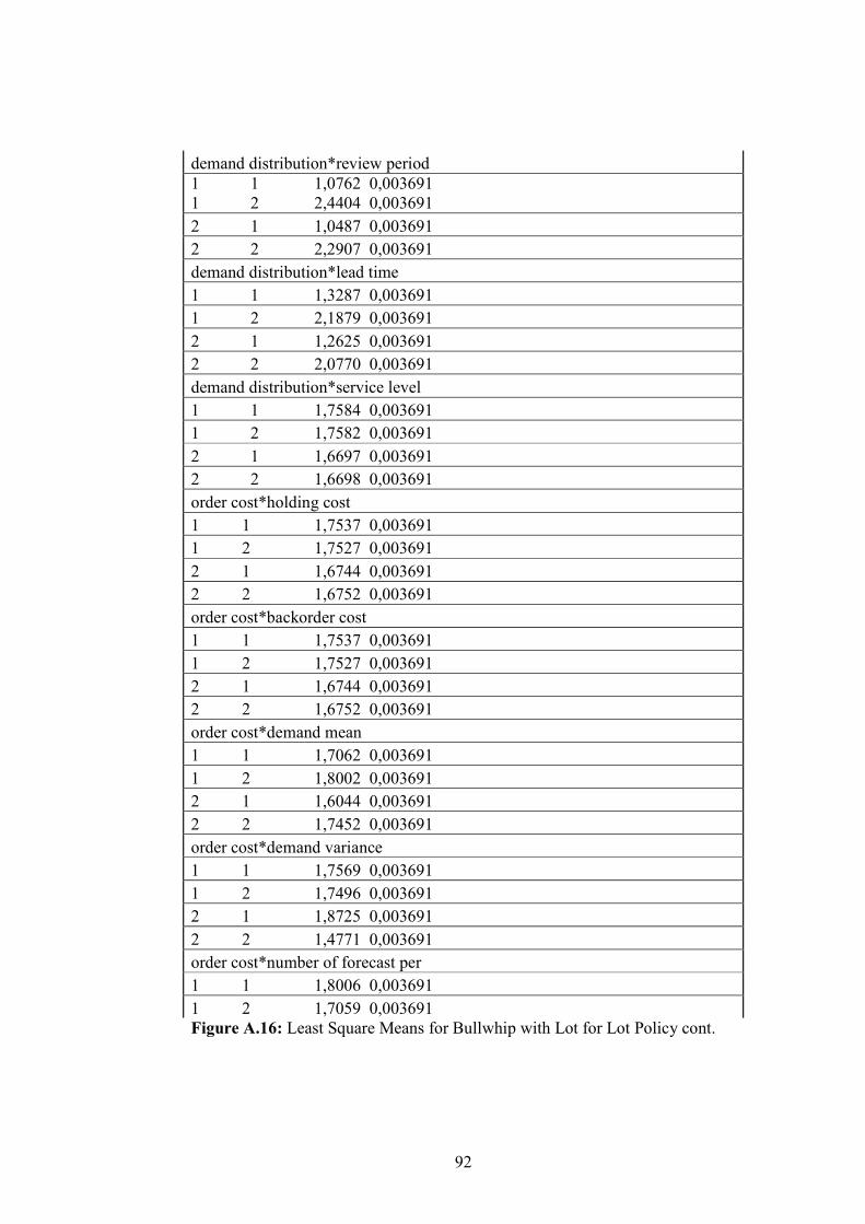
92

demand distribution*review period

1 1 1,0762 0,003691

1 2 2,4404 0,003691

2 1 1,0487 0,003691

2 2 2,2907 0,003691

demand distribution*lead time

1 1 1,3287 0,003691

1 2 2,1879 0,003691

2 1 1,2625 0,003691

2 2 2,0770 0,003691

demand distribution*service level

1 1 1,7584 0,003691

1 2 1,7582 0,003691

2 1 1,6697 0,003691

2 2 1,6698 0,003691

order cost*holding cost

1 1 1,7537 0,003691

1 2 1,7527 0,003691

2 1 1,6744 0,003691

2 2 1,6752 0,003691

order cost*backorder cost

1 1 1,7537 0,003691

1 2 1,7527 0,003691

2 1 1,6744 0,003691

2 2 1,6752 0,003691

order cost*demand mean

1 1 1,7062 0,003691

1 2 1,8002 0,003691

2 1 1,6044 0,003691

2 2 1,7452 0,003691

order cost*demand variance

1 1 1,7569 0,003691

1 2 1,7496 0,003691

2 1 1,8725 0,003691

2 2 1,4771 0,003691

order cost*number of forecast per

1 1 1,8006 0,003691

1 2 1,7059 0,003691

Figure A.16: Least Square Means for Bullwhip with Lot for Lot Policy cont.

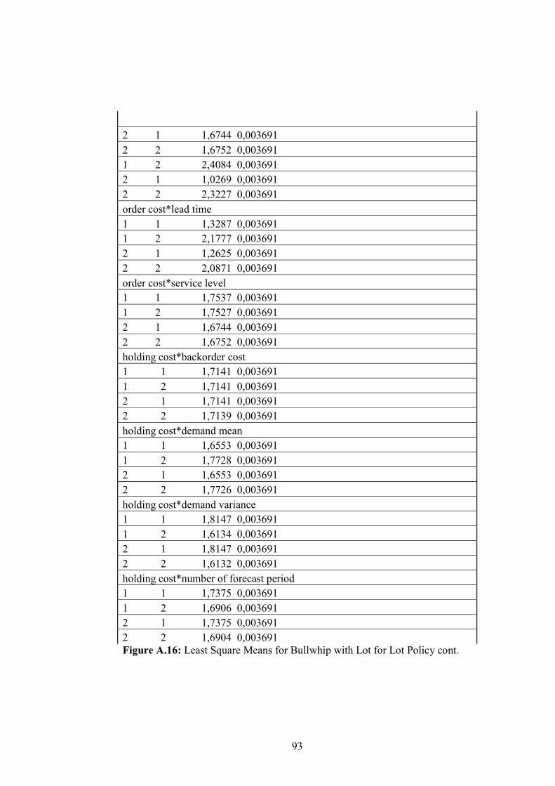
93

2 1 1,6744 0,003691

2 2 1,6752 0,003691

1 2 2,4084 0,003691

2 1 1,0269 0,003691

2 2 2,3227 0,003691

order cost*lead time

1 1 1,3287 0,003691

1 2 2,1777 0,003691

2 1 1,2625 0,003691

2 2 2,0871 0,003691

order cost*service level

1 1 1,7537 0,003691

1 2 1,7527 0,003691

2 1 1,6744 0,003691

2 2 1,6752 0,003691

holding cost*backorder cost

1 1 1,7141 0,003691

1 2 1,7141 0,003691

2 1 1,7141 0,003691

2 2 1,7139 0,003691

holding cost*demand mean

1 1 1,6553 0,003691

1 2 1,7728 0,003691

2 1 1,6553 0,003691

2 2 1,7726 0,003691

holding cost*demand variance

1 1 1,8147 0,003691

1 2 1,6134 0,003691

2 1 1,8147 0,003691

2 2 1,6132 0,003691

holding cost*number of forecast period

1 1 1,7375 0,003691

1 2 1,6906 0,003691

2 1 1,7375 0,003691

2 2 1,6904 0,003691

Figure A.16: Least Square Means for Bullwhip with Lot for Lot Policy cont.

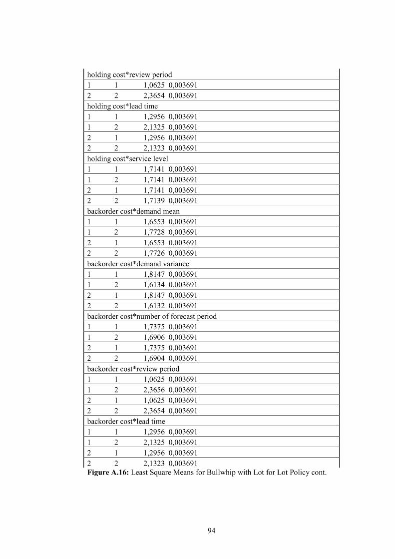
94

holding cost*review period

1 1 1,0625 0,003691

2 2 2,3654 0,003691

holding cost*lead time

1 1 1,2956 0,003691

1 2 2,1325 0,003691

2 1 1,2956 0,003691

2 2 2,1323 0,003691

holding cost*service level

1 1 1,7141 0,003691

1 2 1,7141 0,003691

2 1 1,7141 0,003691

2 2 1,7139 0,003691

backorder cost*demand mean

1 1 1,6553 0,003691

1 2 1,7728 0,003691

2 1 1,6553 0,003691

2 2 1,7726 0,003691

backorder cost*demand variance

1 1 1,8147 0,003691

1 2 1,6134 0,003691

2 1 1,8147 0,003691

2 2 1,6132 0,003691

backorder cost*number of forecast period

1 1 1,7375 0,003691

1 2 1,6906 0,003691

2 1 1,7375 0,003691

2 2 1,6904 0,003691

backorder cost*review period

1 1 1,0625 0,003691

1 2 2,3656 0,003691

2 1 1,0625 0,003691

2 2 2,3654 0,003691

backorder cost*lead time

1 1 1,2956 0,003691

1 2 2,1325 0,003691

2 1 1,2956 0,003691

2 2 2,1323 0,003691

Figure A.16: Least Square Means for Bullwhip with Lot for Lot Policy cont.

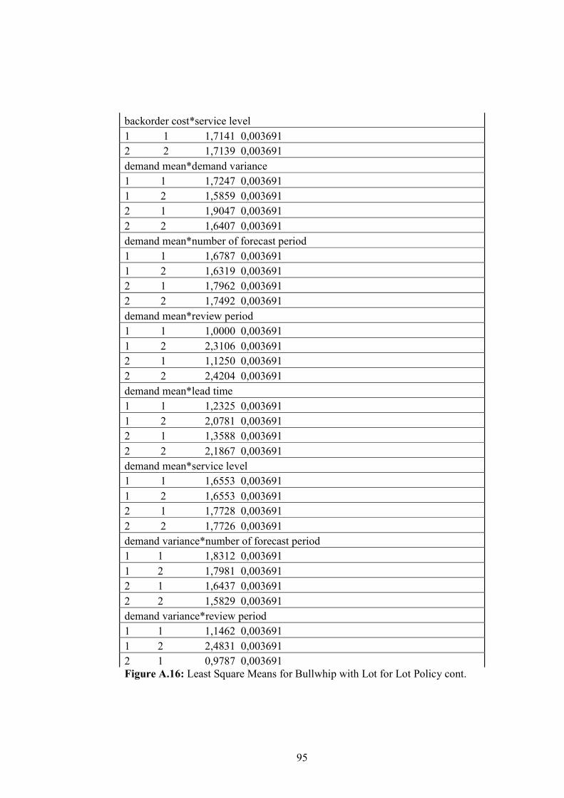
95

backorder cost*service level

1 1 1,7141 0,003691

2 2 1,7139 0,003691

demand mean*demand variance

1 1 1,7247 0,003691

1 2 1,5859 0,003691

2 1 1,9047 0,003691

2 2 1,6407 0,003691

demand mean*number of forecast period

1 1 1,6787 0,003691

1 2 1,6319 0,003691

2 1 1,7962 0,003691

2 2 1,7492 0,003691

demand mean*review period

1 1 1,0000 0,003691

1 2 2,3106 0,003691

2 1 1,1250 0,003691

2 2 2,4204 0,003691

demand mean*lead time

1 1 1,2325 0,003691

1 2 2,0781 0,003691

2 1 1,3588 0,003691

2 2 2,1867 0,003691

demand mean*service level

1 1 1,6553 0,003691

1 2 1,6553 0,003691

2 1 1,7728 0,003691

2 2 1,7726 0,003691

demand variance*number of forecast period

1 1 1,8312 0,003691

1 2 1,7981 0,003691

2 1 1,6437 0,003691

2 2 1,5829 0,003691

demand variance*review period

1 1 1,1462 0,003691

1 2 2,4831 0,003691

2 1 0,9787 0,003691

Figure A.16: Least Square Means for Bullwhip with Lot for Lot Policy cont.

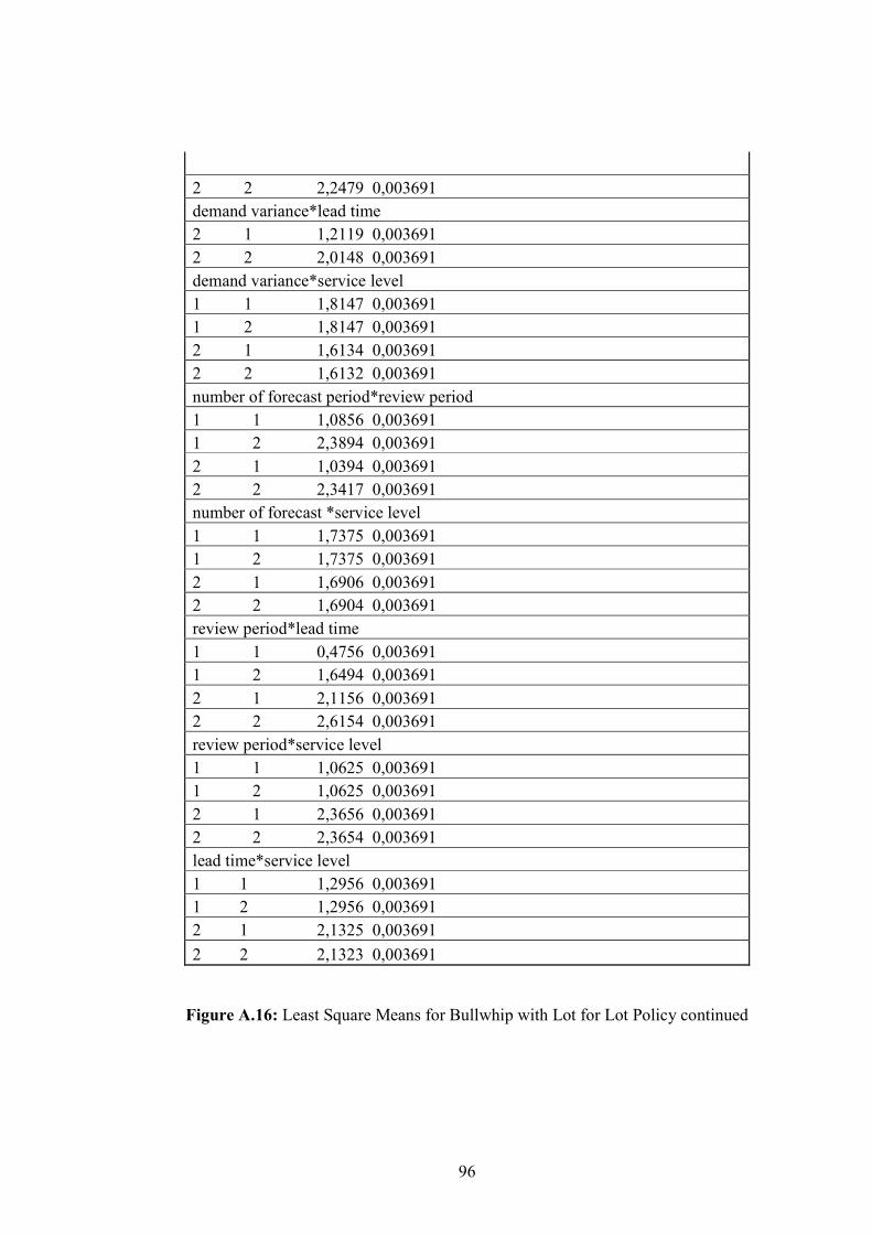
96

2 2 2,2479 0,003691

demand variance*lead time

2 1 1,2119 0,003691

2 2 2,0148 0,003691

demand variance*service level

1 1 1,8147 0,003691

1 2 1,8147 0,003691

2 1 1,6134 0,003691

2 2 1,6132 0,003691

number of forecast period*review period

1 1 1,0856 0,003691

1 2 2,3894 0,003691

2 1 1,0394 0,003691

2 2 2,3417 0,003691

number of forecast *service level

1 1 1,7375 0,003691

1 2 1,7375 0,003691

2 1 1,6906 0,003691

2 2 1,6904 0,003691

review period*lead time

1 1 0,4756 0,003691

1 2 1,6494 0,003691

2 1 2,1156 0,003691

2 2 2,6154 0,003691

review period*service level

1 1 1,0625 0,003691

1 2 1,0625 0,003691

2 1 2,3656 0,003691

2 2 2,3654 0,003691

lead time*service level

1 1 1,2956 0,003691

1 2 1,2956 0,003691

2 1 2,1325 0,003691

2 2 2,1323 0,003691

Figure A.16: Least Square Means for Bullwhip with Lot for Lot Policy continued

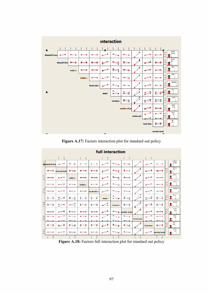
97

Figure A.17: Factors interaction plot for standard out policy

Figure A.18: Factors full interaction plot for standard out policy

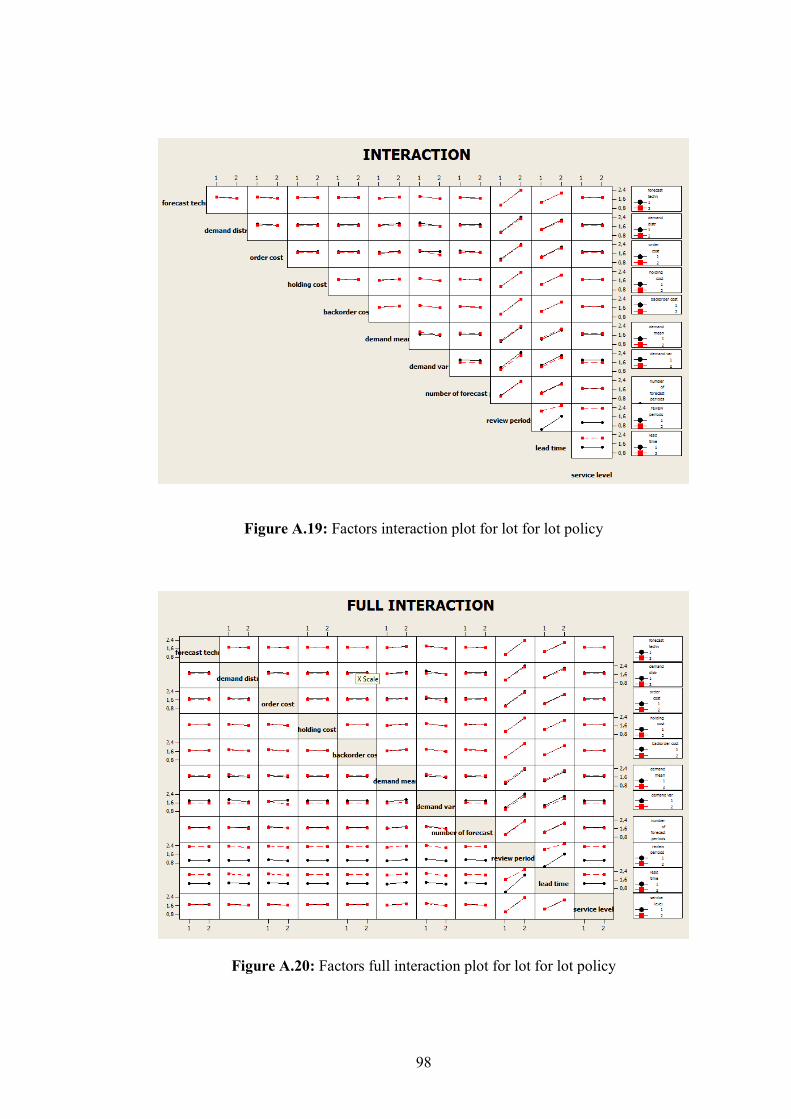
98

Figure A.19: Factors interaction plot for lot for lot policy

Figure A.20: Factors full interaction plot for lot for lot policy