Embed Size (px)
Citation preview

Casualty crash rates for Australian jurisdictions
Jurewicz, C., Bennett, P.
ARRB Group Ltd
email: [email protected]
Abstract
There is a scarcity of information in Australia about casualty crash rates for various types of road
environments. Over a six year period, ARRB carried out an extensive Austroads funded project to
develop a geospatial crash database combining crash, road asset and traffic flow information from
different Australian jurisdictions.
A wealth of crash related information was derived from the database, including casualty crash rates, crash
cost rates (indicative of the cost of road trauma) and relative risks associated with travelling on different
standards of roads. Key relationships between casualty crashes rates and known road safety factors were
explored to demonstrate application of the database. These factors included: traffic volumes, intersection
approach volumes, road hierarchy, terrain and time of day among others.
A number of database outputs have potential for practical application by assisting jurisdictions in road
safety program development and monitoring. Other potential uses were identified and remain to be
explored. ARBB is keen to ensure that researchers and road authorities are aware of this resource and its
potential.
Keywords
Road safety, crash rates, crash costs, safety performance, relative risk, exposure, risk assessment,
database
Introduction
Crash rates, i.e. number of crashes per unit of travel, are a recognised road safety indicator. They are
significant inputs into road safety policy development, assessment of road trauma costs and economic
evaluation. They may be used by practitioners for day-to-day monitoring of the road network safety.
There is a scarcity of information in Australia on casualty crash rates for various stereotypes of roads and
intersections. Much of the existing knowledge in this area has been developed ad-hoc for specific
purposes and remains unpublished. This project aimed to investigate and disseminate information on
crash rates throughout Australia through creation of a nation-wide crash rates database.
During this six-year Austroads project ARRB collected crash data, traffic volume data and road feature
information from most Australian jurisdictions to develop a nation-wide crash rates database. The
database has produced a number of useful road safety indicators to date such as crash rates, relative risks,
crash cost rates and relative costs for a range of road environments in each jurisdiction. Examples of other
practical applications of the database have been produced. Overview of the project results is to be
published in Turner et al. (1) in late 2008.
Methods
With assistance of Austroads member organisations, ARRB defined the aims and carried out the tasks
involved in building a geospatial crash rates database capable of storing data from different jurisdictions.
Specific Aims
A shortlist of areas of interest was prepared and presented to the Austroads stakeholders. The respondents
were requested to indicate the usefulness of the following:
This paper has been peer-reviewedNovember 2008, Adelaide, South Australia2008 Australasian Road Safety Research, Policing and Education Conference
815

• crash rates for different road and intersection stereotypes
• corresponding crash cost rates
• corresponding relative risks and relative costs
• a sample of crash rate functions, safety performance functions and other specific road safety
indicators.
All of the proposed areas were seen as useful by the member authorities in road safety policy and
program evaluation. Therefore, the project proceeded with the data acquisition and analysis along these
lines, within the limits set by the availability of the source data.
Initial Development 2002-2005
The initial four years involved preparation of a pilot database, gathering and understanding of GIS coded
road information from road authorities in different states. The database was developed gradually as
several individual sub-databases in recognition of non-interchangeable definitions of data fields from
different jurisdictions.
Each year, funding was available to acquire, process, check and analyse data sets from individual
jurisdictions. The key element of the database was the geospatial coding of all included information. This
way the detailed road inventory data could be matched with the locations of crashes and the available
AADT information. The database design progress and results were reported back to jurisdictions annually
to assist in their own management and use of crash data.
Development 2005-2008
Between 2005 and 2007 the database was gradually consolidated, expanded and reorganised to produce
the first useful results. One jurisdiction was added to the database, as it developed a geo-coded crash
database at that time. Other jurisdictions, where data was previously of poor quality or simply
unavailable, were able to provide expanded road information data sets, and in particular the AADT
information for various road segments. Several state-controlled crash data sets were again extended and
updated during this stage to maintain currency of the database. This provided a nation-wide coverage,
with exception of the Northern Territory.
Development Process
The method used to derive crash rates information required consolidation of road inventory, traffic and
crash data spatially within a GIS application and extraction of this data to a database application to query
crash rates and other indicators. ArcMap and MapInfo were the GIS applications used to consolidate data
for this study and crash rate queries were created within Access databases.
In summary, the following tasks were performed in order to create the database:
• literature review on the subject to inform the methodology
• approach and data requests to all jurisdictions
• collection and processing of all road, crash and traffic volume data for each jurisdiction
• identification of a method for the annual update of databases with the latest crash data and
AADT information
• development of custom query forms for enhanced data accessibility
• generation of crash rates information for all road and intersection stereotypes.
Crash rates for fatal crashes, serious and other injury crashes, property damage only (PDO)1 crashes and
for casualty crashes (i.e. combined fatal, serious and other injury crashes) were determined from the
available data for each jurisdiction (Northern Territory GIS data was not available). The analysis and
reporting was carried out for road midblock stereotypes (state-state road intersections excluded) and for
1 PDO crashes were excluded from the paper due to the highly inaccurate nature of this variable.
This paper has been peer-reviewedNovember 2008, Adelaide, South Australia2008 Australasian Road Safety Research, Policing and Education Conference
816
Casualty Crash Rates for Australian Jurisdictions Jurewicz and Bennett

state-state road intersection stereotypes. Further analysis was carried out to test for the influence of local
intersections on the midblock crash rates.
Crash Rates
Crash rates indicate the likelihood of a casualty crash for a given road or intersection stereotype. Average
crash rates were expressed in casualty crashes per unit of exposure. The calculations and terminology
used in calculating crash rates for each chosen stereotype are shown in Table 1.
Table 1: Traffic volume and crash rate calculations
Information Calculations
The Average Annual Daily Traffic
(AADT) is a count of all vehicles
travelling in both directions along a road
during an average day. As the crash rates
were determined over a five year period,
the total traffic volumes were calculated
over that period.
TrafVol (5yrs) = AADT x 365 days x 5 years (1)
Crash rates for road midblocks were based
on 100 million vehicle kilometres travelled
(100M VKT).
100M VKT (5yrs) = TrafVol (5yrs) x road length (km) / 108 (2)
Crash rates for intersections were based on
10 million vehicles entering (10M VE).
The sum of all leg traffic volumes was
divided in two as only one traffic flow
direction on each leg was entering the
intersection (equal split was assumed). A
standard approach of 100 m was applied
on all state roads.
10M VE (5yrs) = Sum of all leg TrafVol (5yrs) / 2 / 107 (3)
Midblock crash rates were based on the
number of casualty crashes per 100M
VKT.
Midblock crash rate = Crashes (5yrs) / 100M VKT (5yrs) (4)
Intersection crash rates were based on the
number of casualty crashes per 10M VE. Intersection crash rate = Crashes (5yrs) / 10M VE (5yrs) (5)
Road or intersection stereotypes were defined by either single or multiple attributes derived from the road
inventory data. Thus, at the highest level, crash rates were derived for stereotypes defined by a single
attribute, e.g.: rural, urban, undivided, divided, 3-leg intersections, 4-leg intersections, roundabouts,
traffic signals, etc.
Then, these attributes were combined into logical sub-sets, e.g. rural-undivided, rural-divided, rural-3-leg
intersection-roundabout, etc. Not all attributes were available for all jurisdictions or were directly
comparable. For example, intersection type information was only provided in four of the six jurisdictions.
Many of the attributes varied in their definitions from one jurisdiction to another. To overcome this
problem, some attributes were consolidated into standardised higher-level stereotype definitions for
further analysis. Thus it was possible to report some basic attributes at a nation-wide level. In parallel,
crash rates were also developed using only each jurisdiction’s own attributes (part of forthcoming
Austroads report).
Once crash rates were calculated, ratios of the casualty crash rates were calculated for each group of like
stereotypes. These ratios were referred to as relative risks, as they indicated the likelihood of a casualty
crash for one stereotype compared to the safest stereotype in the group. The following equation shows the
calculation of relative risk for any given stereotype:
This paper has been peer-reviewedNovember 2008, Adelaide, South Australia2008 Australasian Road Safety Research, Policing and Education Conference
817
Casualty Crash Rates for Australian Jurisdictions Jurewicz and Bennett

Relative riskn = Crash raten / Crash rate(lowest) (6)
Thus the stereotype with the lowest casualty crash rate was assigned a relative risk value of 1.00 and all
other stereotypes had a value greater than 1.00.
Crash Cost Rates
Crash cost rates indicate the cost of road trauma and damage borne by the community as a result of road
crashes. They contribute to a more comprehensive understanding of road safety performance by providing
an economic platform for comparison between different road environments and different jurisdictions.
Crash cost rates can be expressed in cents per VKT for midblocks, and in cents per VE for intersections.
Crash cost rates are considered a separate road safety performance indicator, and in this paper, they apply
to different types of road infrastructure. They should be considered alongside other indicators to provide a
full picture of road safety performance of the road transport system. Such indicators include: crash rates
per vehicle-kilometres travelled, per unit of population or per unit of registered vehicles. Crash cost rates
account for differing severity of crashes typically occurring in different road environments. For example,
if two roads have similar casualty crash rates, the one with a higher crash cost rate will generally have
more fatal and serious injury crashes. Such knowledge is crucial in evaluating the effectiveness of
engineering road safety initiatives.
Casualty crash cost rates were calculated by applying the following equation for each chosen road or
intersection stereotype:
Crash cost rate = ∑i (Crashesi x unit crash costi) / Exposure (7)
where:
i = crash severity, i.e. fatal, serious injury, minor injury crash, or as per jurisdiction
definitions.
Crashes = number of crashes of i severity within all midblock segments or intersections
belonging to a particular stereotype, over a five-year period.
Exposure = sum of 100M VKT for all midblock segments, or sum of all 10M VE for all
intersections, belonging to a particular stereotype.
The unit crash costs were obtained from the internal Austroads report by Perovic et al. (2). They were
split by crash severities and by environment (urban/rural). The figures were a June 2007 review of earlier
work by Bureau of Transport Economics (3). The process of estimating the unit crash costs accounted for
such crash-related factors as: type of crash, average number and severity of casualties, funeral and
medical costs, pain and suffering, productive contribution lost, vehicle repair costs, site clean-up costs
and Police, legal and administrative costs.
Relative costs were calculated in a similar way to relative risks, with the lowest cost assigned a value of
1.00. Relative costs provided an easy to understand representation of the road trauma burden of different
road or intersection stereotypes.
Results
The key results for this project were:
• casualty crash rates information for Australian jurisdictions
• examples of practical crash rates information available from the database.
Crash rates information was presented using the following means:
• crash rates in casualty crashes per 100M VKT for midblocks or per 10M VE for intersections
• crash cost rates in cents per VKT or per VE
This paper has been peer-reviewedNovember 2008, Adelaide, South Australia2008 Australasian Road Safety Research, Policing and Education Conference
818
Casualty Crash Rates for Australian Jurisdictions Jurewicz and Bennett
• relative risks
• relative costs.
Casualty Crash Rates for Australian Jurisdictions
Due to the substantial differences in the way crashes and road data are recorded in different jurisdictions,
a higher level of reporting was adopted to provide a common set of road and intersection stereotypes.
Tables 2 and 3 present examples of crash rates information aggregated from jurisdiction level results
(Northern Territory was excluded as GIS road data was not available).
Given the extensive nature of the database, it was not practical to show all possible analyses in this paper.
Three tiers of crash rates information were produced:
• aggregated national overview figures (Tables 2 and 3)
• jurisdiction level figures (Appendix to this paper)
• jurisdiction level figures using the original attributes (to be published in an Austroads report).
Data provided by the authorities contained many different road and traffic attributes which allows further
in-depth investigation of road safety relationships with the road environment. Such analysis can be
facilitated in the future.
National Overview
The method used to combine crash rates from different jurisdictions was a weighted mean based on each
jurisdiction’s proportional contribution to the nation’s road toll, sourced from BTE (3). The figures
presented in Table 2 and Table 3 are aggregates and should not be compared with individual jurisdiction
figures in the Appendix. The national figures could not account for varying levels of injury crash
reporting in different jurisdictions.
The relative risk and relative cost figures are useful in presenting the picture of the relative safety of
different road environments. Relative costs in particular reveal the previously hidden influence of severity
of the crashes occurring in different road environments.
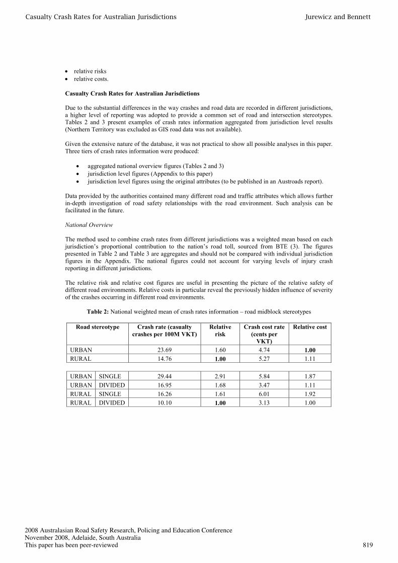
Table 2: National weighted mean of crash rates information – road midblock stereotypes
Road stereotype Crash rate (casualty
crashes per 100M VKT)
Relative
risk
Crash cost rate
(cents per
VKT)
Relative cost
URBAN 23.69 1.60 4.74 1.00
RURAL 14.76 1.00 5.27 1.11
URBAN SINGLE 29.44 2.91 5.84 1.87
URBAN DIVIDED 16.95 1.68 3.47 1.11
RURAL SINGLE 16.26 1.61 6.01 1.92
RURAL DIVIDED 10.10 1.00 3.13 1.00
This paper has been peer-reviewedNovember 2008, Adelaide, South Australia2008 Australasian Road Safety Research, Policing and Education Conference
819
Casualty Crash Rates for Australian Jurisdictions Jurewicz and Bennett

Table 3: National weighted mean of crash rates information – intersection stereotypes
Intersection stereotype Crash rate
(casualty crashes
per 10M VE)
Relative
risk
Crash cost rate
(cents per VE)
Relative cost
URBAN 1.71 1.32 3.24 1.00
RURAL 1.30 1.00 4.11 1.27
URBAN 3 LEG 1.54 1.20 3.00 1.00
URBAN 4 LEG 1.98 1.54 3.75 1.25
RURAL 3 LEG 1.28 1.00 4.09 1.36
RURAL 4 LEG 1.73 1.35 7.06 2.35
URBAN SIGNALS 1.22 1.38 2.41 1.26
URBAN ROUNDABOUT 1.07 1.20 1.91 1.00
URBAN OTHER* 0.93 1.05 2.22 1.16
RURAL SIGNALS 1.08 1.22 2.81 1.48
RURAL ROUNDABOUT 0.89 1.00 2.31 1.21
RURAL OTHER* 0.99 1.12 3.81 2.00 * The term ‘other’ refers to intersections controlled by regulatory signage, i.e. Give Way signs, Stop signs, freeway on-ramp
continuity lines, or traffic regulations (T-intersections). The actual proportions of these within each ‘other’ stereotype were not
known for all jurisdictions.
The above figures are only an example of what can be obtained from the database. The Appendix presents
crash rates information by jurisdiction using the same standardised road and intersection stereotypes as
above.
The above results suggest that on average the social cost of casualty crashes was about 5 cents per each
kilometre travelled. It was more than 10% higher in rural areas than in urban areas, even if the actual
likelihood of being involved in a casualty crash (crash rate) was lower. More in-depth analysis confirmed
that rural single carriageway roads had consistently higher fatal crash rates than any other road stereotype
investigated. This contributed to the higher social costs of road trauma on rural roads. For every vehicle
entering an intersection, there was an underlying 3-4 cents cost associated with casualty crashes. To
appreciate this burden of casualty crashes on Australian road users, the above crash cost rates should be
considered in the context of 19.5 cents per kilometre cost of running a medium size car as suggested by a
2008 review by Royal Automobile Club of Victoria (4).
Based on the calculated crash cost rates, the safest road midblock stereotype was found to be a divided
rural road, followed closely by a divided urban road. The lowest intersection crash rate was attributed to
rural roundabouts; however, the crash cost rate suggested that the urban roundabout resulted in lower
overall cost due to reduced crash severity. The intersection stereotype with the highest crash rate was
urban traffic signals.
Providing the mean crash rates information in Tables 2 and 3 was only one of the benefits of the nation-
wide crash database. The other key benefit was the opportunity to interrogate the crash data and to present
safety performance indicators which could be of use to road safety program managers, road network
planners, road designers and traffic engineers. The following sub-sections present examples of some of
the practical indicators arising from the database. While these examples concentrate primarily on AADT
as an independent variable, there are many other relationships which can be explored on demand.
This paper has been peer-reviewedNovember 2008, Adelaide, South Australia2008 Australasian Road Safety Research, Policing and Education Conference
820
Casualty Crash Rates for Australian Jurisdictions Jurewicz and Bennett

Examples of Practical Application
Crash Rate Functions
Crash rate functions (CRFs) are an example of measuring the influence of traffic flow on the likelihood of
crashes. CRFs are based on plots of crash rates of homogenous road midblock (or intersection) groups
operating at similar AADTs. Analysis of crash data from different jurisdictions suggested that for
midblock road segments of the same type the crash rate remains fairly constant or decreases across the
AADT range. Figure 1 shows a Queensland example based on undivided urban arterials. A significant
variation in crash rates at volumes >20,000 vpd suggests that crash performance on some multilane
undivided roads may be subject to additional influencing factors.
0
5
10
15
20
25
30
0 5,000 10,000 15,000 20,000 25,000 30,000 35,000 40,000
AADT (vpd)
Cra
sh rate
(C
asualty c
rashes p
er 100M
VK
T)
Figure 1: Crash rate function for undivided urban arterials in Queensland
Another example, in Figure 2 shows the effect the number of entering vehicles had on crash rates at 3-leg
rural intersections in Victoria.
Figure 2: Crash rates across the AADT range for 3-leg unsignalised rural arterial intersections in Victoria
R 2 = 0.7046
0.0
0.5
1.0
1.5
2.0
2.5
3.0
3.5
- 2,000 4,000 6,000 8,000 10,000 12,000
Entering AADT (vpd)
Cra
sh
ra
te (
Ca
su
alt
y c
ras
hes
per
10
M V
E)
This paper has been peer-reviewedNovember 2008, Adelaide, South Australia2008 Australasian Road Safety Research, Policing and Education Conference
821
Casualty Crash Rates for Australian Jurisdictions Jurewicz and Bennett

While most crash rates investigated in this project were found to remain reasonably unaffected by the
AADT (i.e. close to the published mean), there were a number of exceptions as shown in Figure 2.
Development of CRFs is therefore an important tool for understanding of safety performance of different
road network elements operating under different traffic conditions.
Safety Performance Functions
An even more useful tool was the safety performance function (SPF). Instead of dealing with the crash
rate, i.e. an average expected number of crashes per unit of exposure, the SPF presents the crash
frequency – average number of crashes per kilometre (or per intersection) over a five year period vs. the
AADT. In other words, average crash rate is the mean gradient of the SPF function.
This format is more immediately useful to practitioners involved in road safety program development or
management. Using the Victorian 3-leg rural unsignalised intersections again as an example scenario,
Figure 3 shows the expected number of crashes over a five year period for a given entering flow AADT
(sum of all entering flows). Four immediate uses of such a function come to mind:
• monitoring of crash performance, e.g. is a ‘problem’ intersection reported by the public above or
below the mean for the given AADT (seek action if it is above)
• for adjusting the expected crash reduction of treatments when they result in increased traffic
volumes
• as a broad indicator of the expected crash numbers should the traffic flow increase over time
• in risk assessment models.
Figure 3: Average 5-year crash frequency at 3-leg unsignalised rural arterial intersections in Victoria
Influence of Major/Minor Intersection Traffic Flows
Measurement of traffic exposure at intersections is more complex than at midblocks due to traffic flows
arriving from several different approaches. The key issue is the conflict between opposing traffic
movements. An optimal way of accounting for exposure to crash risk is crucial for estimation of crash
rates and crash cost rates at intersections.
The crash rates database design allowed investigation of major and minor flows on the frequency of
casualty crashes. Figure 4 shows an example of such analysis for urban 4-leg signalised intersections in
Victoria. This approach can be easily developed into a regression model and used for crash prediction.
Such knowledge may be of use in arterial road planning, e.g. in balancing the frequency of arterial road
intersections with the traffic flow on the side roads.
R2 = 0.89
0.0
0.5
1.0
1.5
2.0
2.5
3.0
3.5
- 2,000 4,000 6,000 8,000 10,000 12,000
Entering AADT (vpd)
Ca
su
alt
y c
ras
he
s p
er
inte
rsec
tio
n (
5 y
ears
)
This paper has been peer-reviewedNovember 2008, Adelaide, South Australia2008 Australasian Road Safety Research, Policing and Education Conference
822
Casualty Crash Rates for Australian Jurisdictions Jurewicz and Bennett

Figure 4: Change in crash frequency at different major and minor intersection leg flows
Influence of Road Hierarchy
The database structure allowed examination of the relative safety of different road hierarchy stereotypes.
Crash performance of undivided rural road segments in South Australia was analysed according to each
segment’s reported road hierarchy classification. A series of SPFs for different roads in the rural
hierarchy are shown in Figure 5.
Figure 5: Casualty crash frequency of rural undivided roads in South Australia, by hierarchy
0
1
2
3
4
5
0 2,000 4,000 6,000 8,000 10,000 12,000
AADT (vpd)
Cas
ua
lty c
ras
he
s / k
m (
5 y
ears
) National Highway Arterial Primary Arterial Secondary Local
R 2 = 0.51
R 2 = 0.57
R 2 = 0.85
R2 = 0.49
0
5
10
15
20
25
30
35
40
45
50
10,000 20,000 30,000 40,000 50,000 60,000 70,000
Major leg AADT (vpd)
Ca
su
alt
y c
ras
he
s p
er
inte
rse
cti
on
(5
years
)
<10,000 vpd
10,000-20,000 vpd
20,000-30,000 vpd
>30,000 vpd
Minor leg AADT
This paper has been peer-reviewedNovember 2008, Adelaide, South Australia2008 Australasian Road Safety Research, Policing and Education Conference
823
Casualty Crash Rates for Australian Jurisdictions Jurewicz and Bennett

The National Highway category had the lowest crash frequency at high traffic volumes, whereas the
Arterial Secondary had a substantially higher crash frequency at the same traffic flows. This confirmed
the common belief that roads on which traffic outgrows their intended function become less safe. This
may be assumed to be related to the engineering standard differences between the road stereotypes, issues
such as alignment, delineation and presence of sealed shoulders.
Influence of Terrain
As an example of applying the road inventory data for crash rate analysis, the NSW crash data was used
to produce an SPF for different types of terrain for undivided urban roads. Figure 6 shows the results for
such roads in flat and undulating terrain. The AADT range was truncated at 20,000 vpd to provide clearer
results (an approximate capacity of undivided two-lane urban roads). Multilane undivided roads appear
above that value and provide a different relationship.
Figure 6: Crash frequency for different terrains for undivided urban arterial roads, based on NSW data
Influence of Time of Day
In-depth analysis of jurisdiction casualty crash details contained in the database allowed development of
crash rate graphs by time of day. Time of day is a proxy for traffic congestion (peak/off-peak) and road
user behaviour (higher speeds at night, intoxication). Analysis of the crash rates rather than crash
frequencies was carried out to account for the different traffic flows at different times.
Figures 7 and 8 illustrate the changes in crash rates for road midblocks and intersections, based on
Victorian data. It is worth noting, that the crash rates were highest during the day-time off-peak period.
Possible causes for this include the combination of higher average speeds, commercial activity and
increased presence of pedestrians. Analysis of crash costs would provide further insight into the impact of
the time of day on road trauma. This could be a subject of future analysis.
0
2
4
6
8
10
12
14
16
18
5,000 10,000 15,000 20,000 25,000
AADT (vpd)
Ca
su
alt
y c
rash
es /
km
(5
ye
ars
) Flat Undulating
This paper has been peer-reviewedNovember 2008, Adelaide, South Australia2008 Australasian Road Safety Research, Policing and Education Conference
824
Casualty Crash Rates for Australian Jurisdictions Jurewicz and Bennett

Figure 7: Average crash rates for midblock road sections based on the time of day (Victorian data)
Figure 8: Average crash rates for intersections based on the time of day (Victorian data)
Analysis of Crash Types
Selected crash types can be analysed as a function of the traffic flow across the network or for a particular
road or intersection stereotype. Figure 9 shows an SPF for head-on crashes. It is clear that the frequency
of crashes strongly increases with the traffic flow (R2 of 0.96). Figure 10 shows that the crash rate was
relatively independent of the AADT (R2 of only 0.19), typical of general midblock CRF results.
Development of a specific-use SPF relationship (e.g. head-on crashes, run-off-road crashes, wet weather
crashes, etc.) may assist jurisdictions in improved analysis of their road network elements by introducing
an exposure sensitivity. Practitioners may use the regression equation to check if a series of crashes
observed at one location is in fact below or above the expected value. Such insight may prove useful in
decisions about further investigation and project funding.
0
5
10
15
20
25
30
35
6pm - 7am 7am - 10am 10am - 3pm 3pm - 6pm
Time of day
Cra
sh
rate
(c
as
ua
lty c
ras
hes
per
100
M V
KT
)
Inner Metro Outer Metro Rural
0.0
0.5
1.0
1.5
2.0
2.5
3.0
6pm - 7am 7am - 10am 10am - 3pm 3pm - 6pm
Time of day
Cra
sh
ra
te (
ca
su
alt
y c
ras
he
s p
er
10
M V
E)
Inner Metro Outer Metro Rural
This paper has been peer-reviewedNovember 2008, Adelaide, South Australia2008 Australasian Road Safety Research, Policing and Education Conference
825
Casualty Crash Rates for Australian Jurisdictions Jurewicz and Bennett

Figure 9: Expected head-on crashes frequency based on Victorian data for undivided rural arterial roads
Figure 10: Expected head-on crash rate based on Victorian data for undivided rural arterial roads
Relative Risk Functions
Many design guidelines and risk assessment methods utilise the relative risk to express the changing
likelihood of casualty crashes as a result of a particular feature. Any of the above crash rate functions
could be easily converted into a risk function by taking the lowest crash rate as the baseline risk of 1.0
CF h-o = 2E-05 AADT 1.3
R 2 = 0.96
0
2
4
6
8
10
12
- 5,000 10,000 15,000 20,000 25,000
AADT (vpd)
He
ad
-on
cra
sh
es
/ 1
0 k
m (
5 y
ears
)
R 2 = 0.19
0.0
0.5
1.0
1.5
2.0
2.5
3.0
- 5,000 10,000 15,000 20,000 25,000
AADT (vpd)
Hea
d-o
n c
ras
h r
ate
(c
as
ua
lty
cra
sh
es
per
10
0M
VK
T)
This paper has been peer-reviewedNovember 2008, Adelaide, South Australia2008 Australasian Road Safety Research, Policing and Education Conference
826
Casualty Crash Rates for Australian Jurisdictions Jurewicz and Bennett

and using it as a ratio denominator. Figure 11 shows an example how the risk of a casualty crash
decreases with increasing flow.
Figure 11: Relative crash risks for undivided urban arterial roads in NSW (flat terrain) vs. AADT
Influence of Local Intersection Crashes on Midblock Crash Rates
The data held by jurisdictions generally contained the traffic flow information for the state-controlled
road network. Local road traffic and GIS information was either missing or was held by the local
governments and was thus unavailable. Hence, state-local road intersections had to be ignored in the
midblock crash rate calculations and any crashes occurring at such locations were included in the
midblock sample. This practice is common in crash rate analysis literature. Nevertheless, the influence of
state-local intersections was suspected to be significant, particularly in the urban environments.
Engineering ‘folklore’ suggested that in urban environments, road midblock segments have relatively few
crashes and that most crashes occur at either state-state road intersections or at state-local road
intersections.
The crash rates database allowed this hypothesis to be tested by separating the influence of state-local
road intersections on the midblock crash rates. This was achieved by filtering out from the midblock
crashes sample any crashes spatially identified by Police as occurring within 10 m of an intersection.
Those crashes that remained in the sample were thus identified as true midblock crashes. Figure 12
illustrates the significant difference in the crash rates when all state-local road intersection crashes have
been removed.
0.0
0.5
1.0
1.5
2.0
2.5
3.0
3.5
4.0
- 5,000 10,000 15,000 20,000 25,000
AADT (vpd)
Re
lati
ve r
isk
This paper has been peer-reviewedNovember 2008, Adelaide, South Australia2008 Australasian Road Safety Research, Policing and Education Conference
827
Casualty Crash Rates for Australian Jurisdictions Jurewicz and Bennett
0
10
20
30
40
50
60
70
80
0 10,000 20,000 30,000 40,000 50,000 60,000 70,000 80,000 90,000
AADT (vpd)
Cra
sh rate
(C
asualty c
rashes p
er 100M
VK
T)
Typical midblock crash rate
True midblock crash rate (no intersections)
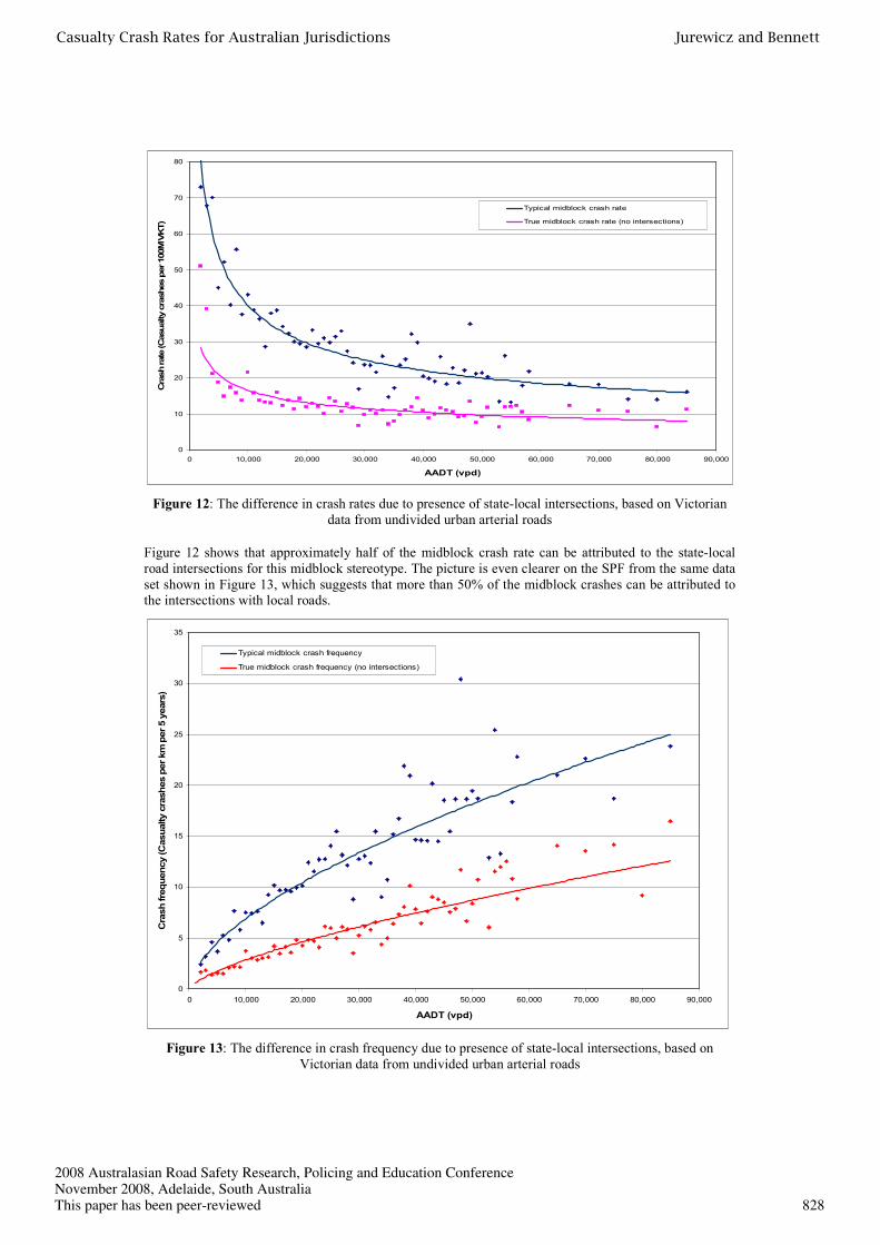
Figure 12: The difference in crash rates due to presence of state-local intersections, based on Victorian
data from undivided urban arterial roads
Figure 12 shows that approximately half of the midblock crash rate can be attributed to the state-local
road intersections for this midblock stereotype. The picture is even clearer on the SPF from the same data
set shown in Figure 13, which suggests that more than 50% of the midblock crashes can be attributed to
the intersections with local roads.
0
5
10
15
20
25
30
35
0 10,000 20,000 30,000 40,000 50,000 60,000 70,000 80,000 90,000
AADT (vpd)
Cra
sh fre
quency (C
asualty c
rash
es p
er km
per 5 y
ears
)
Typical midblock crash frequency
True midblock crash frequency (no intersections)
Figure 13: The difference in crash frequency due to presence of state-local intersections, based on
Victorian data from undivided urban arterial roads
This paper has been peer-reviewedNovember 2008, Adelaide, South Australia2008 Australasian Road Safety Research, Policing and Education Conference
828
Casualty Crash Rates for Australian Jurisdictions Jurewicz and Bennett

Analysis of Accuracy
The SPFs and CRFs present mean values for small AADT ranges. The results can be subjected to
rigorous error analysis to provide an indication of their robustness. While a detailed review of different
error analysis methods is a subject for another project, the authors chose one of the simplest applicable
methods to provide an example of the accuracy of the information derived from the crash rates database.
Along with estimating the crash rate as a single value, an interval likely to include that value can also be
given. Thus the 95% confidence interval (95CL) is described by the upper and lower bound values
between which there is a 95% chance of finding the true mean value. The narrower the interval, the more
reliable the value is. In case of the Poisson distribution (applicable to crash events) the 95% interval of the
crash rate may be represented simply as:
95CL = ± 1.96 (number of crashes)0.5 / Exposure from the mean value (8)
The example from Figure 2 can be re-plotted showing the upper and lower bounds of the results, as
shown on Figure 14. As it can be observed, the relationship begins to break down at the higher traffic
volumes – the 95CL spans the zero. This is usually a sign that the number of crashes in the sample is too
low to provide robust crash rate information.
Figure 14: The 95% confidence interval for a crash rate function for 3-leg unsignalised rural intersections
in Victoria
Discussion
The crash rate information (crash rates, crash cost rates, relative risks and relative costs) obtained varied
from state to state. Though none of the jurisdictions could provide a full set of traffic flow data for the
entire state road network, the coverage for each of the jurisdictions was large enough to have confidence
in most of the rates for stereotypes defined by the attributes in Tables 2 and 3 and in the Appendix.
The differences in the data sources, road attributes and their definitions, and in extraction methods should
be kept in mind when comparing crash rate information results. Examples of these variations are as
follows:
• the percentage of the total road network included in the data sets, road attributes and traffic
volume coverage across each jurisdiction
• different classification of roads across jurisdictions
• different classification of crash severities
R2 = 0.7046
0.0
0.5
1.0
1.5
2.0
2.5
3.0
3.5
4.0
4.5
2,000 4,000 6,000 8,000 10,000 12,000
Entering AADT (vpd)
Cra
sh
ra
te (
ca
su
alt
y c
ras
he
s p
er
10
M V
E)
This paper has been peer-reviewedNovember 2008, Adelaide, South Australia2008 Australasian Road Safety Research, Policing and Education Conference
829
Casualty Crash Rates for Australian Jurisdictions Jurewicz and Bennett

• different reporting rates between jurisdictions, especially for injury crashes
• environment classification as urban, outer urban or rural varied between jurisdictions; some had
to be assumed on the basis of speed limit due to lack of other information
• traffic volume records and/or estimates – some jurisdictions had up-to-date data, others provided
updated estimates based on old counts.
These variations in the data made it too difficult at this stage to integrate the jurisdiction data into a
central Australian database. The task of consolidating the road and crash information at a national level is
possible and should be considered as a strategic long-term project with benefits for road infrastructure
planning and road safety policy at state and national levels. In particular, development of a KSI index
(killed and seriously injured) similar to that used in the UK would be of key importance in monitoring the
progress towards the ‘safe system’ in road transport, the aim of the National Road Safety Strategy.
A step toward achieving a national uniformity of crash rates would be an audit of the fatal and injury
under-reporting levels in each jurisdiction and development of appropriate adjustment factors for each
jurisdiction. There has been no recent in-depth Australian research in this field.
It was decided not to include property damage only (PDO) crash rates in this paper. The under-reporting
rates were known to be very high. The crash reporting requirements also varied between jurisdictions
(e.g. the estimated cost of damage requiring reporting). For those reasons, this useful severity category
could not be reported or compared accurately.
Analysis carried out as part of the project highlighted an ongoing issue with crash and road data
availability. Most jurisdiction data sets allowed only limited analysis of factors influencing road safety
performance.
In analysis of intersection crash rates information, only the intersections for which traffic volumes were
known on all legs were included in the sample. Thus, for some jurisdictions the sample size for
intersections was lower than desired due to lack of traffic flow data.
Reporting of crash information across Australian jurisdictions appeared to decline over the duration of the
project. One jurisdiction combined the reporting of serious and minor injuries into one category. Two
other jurisdictions experienced reporting delays of 12-18 months. Unavailability of up-to-date and reliable
crash information will impact the future monitoring of road safety performance and may lead to wrong
conclusions regarding the economic benefits of road safety programs. It should be noted, however, that
the road asset information has generally improved over the duration of the project.
There are numerous opportunities to further utilise and develop the crash rates database. Some of the
areas where further uses and developments have been identified are:
• use of relative risks in risk assessment models and programs
• geo-spatial analysis of crash costs, e.g. combined with socio-economic factors, climatic
conditions, road expenditure, maintenance, etc
• development of multi-variable crash prediction models so that safety consequences of
engineering changes can be appreciated before funding decisions are made
• in road safety policy development – to target issues or areas of poor crash performance
• development and economic evaluation of road safety programs
• Road Safety Impact Statement / Assessment methods
• improved monitoring of the progress towards the goals of the National Road Safety Strategy.
This paper has been peer-reviewedNovember 2008, Adelaide, South Australia2008 Australasian Road Safety Research, Policing and Education Conference
830
Casualty Crash Rates for Australian Jurisdictions Jurewicz and Bennett

References
1. Turner B, Roper P, Jurewicz C, Cairney C, Tziotis M, ‘Road Safety Engineering Risk
Assessment Stage 6: Overview of Research’, in press internal Austroads report, Sydney
Australia, 2008.
2. Perovic J, Evans C, Lloyd B, Tsolakis D, ‘Update of RUC Unit Values to June 2007’, internal
Austroads report IR156/08, Sydney, Australia, 2007.
3. Bureau of Transport Economics, ‘Road crash costs in Australia’, report 102, Bureau of Transport
Economics, Canberra, ACT, 2000.
4. RACV, ‘Vehicle operating cost results 2008’, Melbourne, Victoria, viewed on 2 July 2008
<http://www.racv.com.au/wps/wcm/resources/file/ebcbb90bd4187b0/medium.pdf>.
This paper has been peer-reviewedNovember 2008, Adelaide, South Australia2008 Australasian Road Safety Research, Policing and Education Conference
831
Casualty Crash Rates for Australian Jurisdictions Jurewicz and Bennett

APPENDIX
The appendix shows the second tier of presented crash rates information – the high level attributes by
jurisdiction. At this level of reporting, several stereotypes suffered from small sample size which affected
the accuracy of the results. A large 95% confidence interval indicates that the result is not robust. The
same can be concluded if the lower end of the confidence interval falls below the zero.
New South Wales
The following crash rates have been produced for New South Wales. Greater detail of attributes and
results exists within the database. It is possible to perform more specific analysis on request.
Table A1: New South Wales crash rates – road midblock stereotypes
Road stereotype Crash rate
(casualty
crashes per
100M VKT)
95%
confidence
interval
Relative
risk
Crash cost
rate (cents
per VKT)
Relative
cost
URBAN 29.37 (29.06; 29.68) 2.29 5.77 1.41
RURAL 12.82 (12.57; 13.07) 1.00 4.08 1.00
URBAN SINGLE 35.89 (35.33; 36.45) 3.37 7.12 2.46
URBAN DIVIDED 25.58 (25.22; 25.94) 2.40 4.99 1.73
RURAL SINGLE 13.44 (13.15; 13.73) 1.26 4.42 1.53
RURAL DIVIDED 10.65 (10.17; 11.13) 1.00 2.89 1.00
Table A2: New South Wales crash rates – intersection stereotypes
Intersection stereotype Crash rate
(casualty
crashes per
10M VE)
95%
confidence
interval
Relative
risk
Crash cost
rate (cents
per VE)
Relative
cost
URBAN 1.49 (1.45; 1.53) 1.51 2.66 1.06
RURAL 0.99 (0.87; 1.11) 1.00 2.52 1.00
URBAN 3 LEG 1.50 (1.45; 1.55) 1.69 2.65 1.06
URBAN 4 LEG 1.46 (1.39; 1.53) 1.64 2.67 1.07
RURAL 3 LEG 1.00 (0.88; 1.12) 1.12 2.49 1.00
RURAL 4 LEG 0.89 (0.45; 1.33) 1.00 2.86 1.15
This paper has been peer-reviewedNovember 2008, Adelaide, South Australia2008 Australasian Road Safety Research, Policing and Education Conference
832
Casualty Crash Rates for Australian Jurisdictions Jurewicz and Bennett

Victoria
The crash rates information for Victoria was extended by inclusion of intersection control stereotypes.
Greater detail of attributes and results exists within the database. It is possible to perform more specific
analysis on request.
Table A3: Victorian crash rates – road midblock stereotypes
Road stereotype Crash rate
(casualty
crashes per
100M VKT)
95%
confidence
interval
Relative
risk
Crash cost
rate (cents
per VKT)
Relative
cost
URBAN 23.22 (22.92; 23.52) 1.42 4.25 1.00
RURAL 16.31 (15.95; 16.67) 1.00 4.87 1.15
URBAN SINGLE 32.12 (31.69; 32.55) 5.77 5.84 5.26
URBAN DIVIDED 5.57 (5.32; 5.82) 1.00 1.11 1.00
RURAL SINGLE 18.57 (18.14; 19.00) 3.33 5.71 5.14
RURAL DIVIDED 8.65 (8.11; 9.19) 1.55 2.05 1.85
Table A4: Victorian crash rates – intersection stereotypes
Intersection stereotype Crash rate
(casualty
crashes per
10M VE)
95%
confidence
interval
Relative
risk
Crash cost
rate (cents
per VE)
Relative
cost
URBAN 2.01 (1.96; 2.06) 1.27 3.01 1.00
RURAL 1.58 (1.44; 1.72) 1.00 3.66 1.22
URBAN 3 LEG 1.87 (1.80; 1.94) 1.26 2.80 1.00
URBAN 4 LEG 2.11 (2.04; 2.18) 1.43 3.16 1.13
RURAL 3 LEG 1.60 (1.42; 1.78) 1.08 4.07 1.45
RURAL 4 LEG 1.48 (1.27; 1.69) 1.00 2.93 1.05
URBAN SIGNALS 2.04 (1.99; 2.09) 1.39 3.02 2.03
URBAN ROUNDABOUT 1.50 (1.31; 1.69) 1.02 1.49 1.00
URBAN OTHER 1.86 (1.72; 2.00) 1.27 3.38 2.27
RURAL SIGNALS 1.47 (1.28; 1.66) 1.00 2.57 1.72
RURAL ROUNDABOUT 1.71 (1.33; 2.09) 1.16 2.68 1.80
RURAL OTHER 1.69 (1.46; 1.92) 1.15 5.49 3.68
This paper has been peer-reviewedNovember 2008, Adelaide, South Australia2008 Australasian Road Safety Research, Policing and Education Conference
833
Casualty Crash Rates for Australian Jurisdictions Jurewicz and Bennett

Queensland
The following crash rates information have been produced for Queensland. Greater detail of attributes and
results exists within the database. It is possible to perform more specific analysis on request.
Table A5: Queensland crash rates – road midblock stereotypes
Road stereotype Crash rate
(casualty
crashes per
100M VKT)
95%
confidence
interval
Relative
risk
Crash cost
rate (cents
per VKT)
Relative
cost
URBAN 12.80 (12.24; 13.36) 1.00 5.38 1.00
RURAL 13.43 (13.02; 13.84) 1.05 7.04 1.31
URBAN SINGLE 13.38 (12.59; 14.17) 1.56 5.73 1.31
URBAN DIVIDED 12.19 (11.41; 12.97) 1.42 5.02 1.15
RURAL SINGLE 15.28 (14.76; 15.8) 1.78 8.06 1.84
RURAL DIVIDED 8.59 (7.96; 9.22) 1.00 4.38 1.00
Table A6: Queensland crash rates – intersection stereotypes
Intersection stereotype Crash rate
(casualty
crashes per
10M VE)
95%
confidence
interval
Relative
risk
Crash cost
rate (cents
per VE)
Relative
cost
URBAN 1.55 (1.26; 1.84) 1.00 5.9 1.00
RURAL 1.80 (1.51; 2.09) 1.16 9.34 1.58
URBAN 3 LEG 1.45 (1.14; 1.76) 1.00 5.62 1.00
URBAN 4 LEG 2.00 (1.24; 2.76) 1.38 7.10 1.26
RURAL 3 LEG 1.69 (1.41; 1.97) 1.17 8.67 1.54
RURAL 4 LEG 4.29 (2.12; 6.46) 2.96 24.76 4.41
URBAN SIGNALS 1.89 (1.27; 2.51) 1.36 6.54 1.17
URBAN ROUNDABOUT 1.67 (0.76; 2.58) 1.20 6.13 1.10
URBAN OTHER 1.39 (1.05; 1.73) 1.00 5.59 1.00
RURAL SIGNALS 2.32 (2.05; 2.59) 1.67 8.56 1.53
RURAL ROUNDABOUT 1.47 (0.60; 2.34) 1.06 6.72 1.20
RURAL OTHER 1.83 (1.53; 2.13) 1.32 9.59 1.72
This paper has been peer-reviewedNovember 2008, Adelaide, South Australia2008 Australasian Road Safety Research, Policing and Education Conference
834
Casualty Crash Rates for Australian Jurisdictions Jurewicz and Bennett

South Australia
The following crash rates information was produced for South Australia. Greater detail of attributes and
results exists within the database. It is possible to perform more specific analysis on request.
Table A7: South Australian crash rates– road midblock stereotypes
Road stereotype Crash rate
(casualty
crashes per
100M VKT)
95%
confidence
interval
Relative
risk
Crash cost
rate (cents
per VKT)
Relative
cost
URBAN 35.35 (34.66; 36.04) 1.92 3.90 1.00
RURAL 18.37 (17.83; 18.91) 1.00 5.68 1.46
URBAN SINGLE 44.64 (43.11; 46.17) 4.53 5.05 2.11
URBAN DIVIDED 32.10 (31.33; 32.87) 3.26 3.5 1.46
RURAL SINGLE 21.96 (21.26; 22.66) 2.23 7.07 2.96
RURAL DIVIDED 9.85 (9.13; 10.57) 1.00 2.39 1.00
Table A8: South Australian crash rates – intersection stereotypes
Intersection stereotype Crash rate
(casualty
crashes per
10M VE)
95%
confidence
interval
Relative
risk
Crash cost
rate (cents
per VE)
Relative
cost
URBAN 2.42 (2.35; 2.49) 1.74 2.27 1.00
RURAL 1.39 (1.27; 1.51) 1.00 3.28 1.44
URBAN 3 LEG 1.90 (1.81; 1.99) 1.43 1.92 1.00
URBAN 4 LEG 2.82 (2.72; 2.92) 2.12 2.56 1.33
RURAL 3 LEG 1.33 (1.20; 1.46) 1.00 3.23 1.68
RURAL 4 LEG 1.67 (1.34; 2.00) 1.26 3.57 1.86
URBAN SIGNALS 2.65 (2.57; 2.73) 2.35 2.45 1.74
URBAN ROUNDABOUT 3.05 (2.63; 3.47) 2.70 2.56 1.82
URBAN OTHER 1.22 (1.10; 1.34) 1.08 1.41 1.00
RURAL SIGNALS 1.95 (1.37; 2.53) 1.73 3.73 2.65
RURAL ROUNDABOUT 1.13 (0.74; 1.52) 1.00 2.16 1.53
RURAL OTHER 1.36 (1.23; 1.49) 1.20 3.34 2.37
This paper has been peer-reviewedNovember 2008, Adelaide, South Australia2008 Australasian Road Safety Research, Policing and Education Conference
835
Casualty Crash Rates for Australian Jurisdictions Jurewicz and Bennett

Western Australia
An example of crash rates information derived from the database is provided below. Greater detail of
attributes and results for Western Australia exists within the database. It is possible to perform more
specific analysis on request.
Table A9: Western Australia crash rates – road midblock stereotypes
Road stereotype Crash rate
(casualty
crashes per
100M VKT)
95%
confidence
interval
Relative
risk
Crash cost
rate (cents
per VKT)
Relative
cost
URBAN 21.81 (20.93; 22.69) 1.53 3.61 1.00
RURAL 14.29 (13.86; 14.72) 1.00 5.75 1.59
URBAN SINGLE 24.72 (23.28; 26.16) 1.80 4.26 1.37
URBAN DIVIDED 19.64 (18.53; 20.75) 1.43 3.12 1.00
RURAL SINGLE 13.72 (13.18; 14.26) 1.00 6.21 1.99
RURAL DIVIDED 15.17 (14.46; 15.88) 1.11 5.04 1.62
Table A10: Western Australia crash rates – intersection stereotypes
Intersection stereotype Crash rate
(casualty
crashes per
10M VE)
95%
confidence
interval
Relative
risk
Crash cost
rate (cents
per VE)
Relative
cost
URBAN 1.32 (1.21; 1.43) 3.57 1.90 1.68
RURAL 0.37 (0.33; 0.41) 1.00 1.13 1.00
URBAN 3 LEG 0.84 (0.73; 0.95) 3.65 1.16 1.59
URBAN 4 LEG 2.29 (2.04; 2.54) 9.96 3.39 4.64
RURAL 3 LEG 0.43 (0.38; 0.48) 1.87 1.29 1.77
RURAL 4 LEG 0.23 (0.17; 0.29) 1.00 0.73 1.00
This paper has been peer-reviewedNovember 2008, Adelaide, South Australia2008 Australasian Road Safety Research, Policing and Education Conference
836
Casualty Crash Rates for Australian Jurisdictions Jurewicz and Bennett

Tasmania
A sample of Tasmanian crash rate information has been developed. Greater detail of attributes and results
exists within the database. It is possible to perform more specific analysis on request.
Table A11: Tasmanian crash rates – road midblock stereotypes
Road stereotype Crash rate
(casualty
crashes per
100M VKT)
95%
confidence
interval
Relative
risk
Crash cost
rate (cents
per VKT)
Relative
cost
URBAN 20.23 (18.68; 21.78) 1.20 2.91 1.00
RURAL 16.92 (16.17; 17.67) 1.00 4.60 1.58
URBAN SINGLE 22.61 (20.21; 25.01) 2.29 3.69 2.12
URBAN DIVIDED 18.18 (16.18; 20.18) 1.84 2.24 1.29
RURAL SINGLE 18.96 (18.06; 19.86) 1.92 5.43 3.12
RURAL DIVIDED 9.86 (8.66; 11.06) 1.00 1.74 1.00
Table A12: Tasmanian crash rates – intersection stereotypes
Intersection stereotype Crash rate
(casualty
crashes per
10M VE)
95%
confidence
interval
Relative
risk
Crash cost
rate (cents
per VE)
Relative
cost
URBAN 0.85 (0.56; 1.04) 1.06 1.00 1.00
RURAL 0.80 (0.65; 1.03) 1.00 1.89 1.89
URBAN 3 LEG 0.84 (0.59; 1.09) 1.91 0.96 1.00
URBAN 4 LEG 1.51 (0.03; 2.99) 3.43 1.86 1.94
RURAL 3 LEG 0.83 (0.64; 1.02) 1.89 1.79 1.86
RURAL 4 LEG 0.44 (-0.06; 0.94) 1.00 3.25 3.39
This paper has been peer-reviewedNovember 2008, Adelaide, South Australia2008 Australasian Road Safety Research, Policing and Education Conference
837
Casualty Crash Rates for Australian Jurisdictions Jurewicz and Bennett

Australian Capital Territory
Greater detail of ACT attributes and results exists within the database. It is possible to perform more
specific analysis on request.
Table A13: ACT crash rates – road midblock stereotypes
Road stereotype Crash rate
(casualty
crashes per
100M VKT)
95%
confidence
interval
Relative
risk
Crash cost
rate (cents
per VKT)
Relative
cost
URBAN 4.80 (4.34; 5.26) 1.00 1.02 1.00
RURAL 19.69 (15.48; 23.9) 4.10 5.41 5.30
URBAN SINGLE 6.00 (5.17; 6.83) 1.49 1.26 1.48
URBAN DIVIDED 4.04 (3.49; 4.59) 1.00 0.86 1.01
RURAL SINGLE 20.5 (16.06; 24.94) 5.07 5.71 6.72
RURAL DIVIDED 7.52 (-2.9; 17.94) 1.86 0.85 1.00
Table A14: ACT crash rates – intersection stereotypes
Intersection stereotype Crash rate
(casualty
crashes per
10M VE)
95%
confidence
interval
Relative
risk
Crash cost
rate (cents
per VE)
Relative
cost
URBAN 0.62 (0.54; 0.7) 1.00 0.99 1.00
RURAL 2.47 (-0.32; 5.26) 3.98 2.78 2.81
URBAN 3 LEG 0.58 (0.48; 0.68) 1.00 0.89 1.27
URBAN 4 LEG 0.69 (0.56; 0.82) 1.19 1.16 1.66
RURAL 3 LEG 2.47 (-0.32; 5.26) 4.26 2.78 3.97
RURAL 4 LEG 0.62 (0.19; 1.05) 1.07 0.70 1.00
This paper has been peer-reviewedNovember 2008, Adelaide, South Australia2008 Australasian Road Safety Research, Policing and Education Conference
838
Casualty Crash Rates for Australian Jurisdictions Jurewicz and Bennett