NBER WORKING PAPER SERIES

WHAT CAUSED THE RECESSION OF 2008? HINTS FROM LABOR PRODUCTIVITY

Casey Mulligan

Working Paper 14729http://www.nber.org/papers/w14729

NATIONAL BUREAU OF ECONOMIC RESEARCH1050 Massachusetts Avenue

Cambridge, MA 02138February 2009

I appreciate the comments of Gary Becker, Emir Kamenica, Kevin Murphy, Marcus Nunes, and Jesse Shapiro and participants at the January 6, 2009 Money and Banking Workshop at the University of Chicago. I will provide updates on my blog www.panic2008.net. I appreciate the financial support of the George J. Stigler Center for the Study of the Economy and the State.¸ The views expressed herein are those of the author(s) and do not necessarily reflect the views of the National Bureau of Economic Research.

© 2009 by Casey Mulligan. All rights reserved. Short sections of text, not to exceed two paragraphs, may be quoted without explicit permission provided that full credit, including © notice, is given to the source.

What Caused the Recession of 2008? Hints from Labor Productivity Casey Mulligan NBER Working Paper No. 14729 February 2009 JEL No. E24,E32,J22

ABSTRACT

A labor market tautology says that any change in labor usage can be decomposed into a movement along a marginal productivity schedule and a shift of the schedule. I calculate this decomposition for the recession of 2008, assuming an aggregate Cobb-Douglas marginal productivity schedule, and find that all of the decline in employment and hours since December 2007 is a movement along the schedule. This finding suggests that a reduction in labor supply and/or an increase in labor market distortions are major factors in the 2008 recession. The decline in aggregate consumption suggests that the reduction in labor supply (if any) is neither a wealth nor an intertemporal substitution effect. "Sticky real wages" or the emergence of significant work disincentives are possible explanations for these findings.

Casey Mulligan University of Chicago Department of Economics 1126 East 59th Street Chicago, IL 60637 and NBER c-mulligan@uchicago.edu

Financial market chaos has been the main story of 2008, and at roughly the same

time employment and hours have been falling. Both the public and academics have

clamored for government action to alleviate the recession. But identifying the proper

policy response likely requires an understanding of the causes and mechanisms by which

the 2008 recession occurred.

A variety of explanations have been offered for previous recessions: adverse

productivity shocks (Kydland and Prescott, 1982), a surge in the demand for “liquidity”

(Friedman and Schwartz, 1963; Lucas, 2008), a collapse in international trade (Crucini

and Kahn, 1996), and a stock market crash are among them. Which, if any, of these

explanations apply today? This paper begins an answer to the question by decomposing

the 2008 employment reduction into three types of potential “causes”: productivity

shocks that reduce labor and productivity, wealth and intertemporal substitution effects

that reduce labor and raise consumption, and labor distortions and labor preferences that

raise productivity and reduce labor. I conclude that the 2008 recession, like the 2001

recession, is qualitatively different from previous severe recessions because productivity

growth (adjusted for changes in the amount of labor employed) was normal while labor

“supply” (defined more rigorously below) shifted to the left.

Analytically, my decomposition is most like that of Katz and Murphy (1992), who

look at changes over time in the relative amounts and productivity of skilled and

unskilled labor in order to determine the relative importance of supply and demand

shocks. In terms of substance, this paper is about the changes over time in the overall

levels of labor and labor productivity, which raises the possibilities of tax distortions,

wealth effects, and intertemporal substitution effects that would be less important for

understanding one education group’s changes relative to another. In this regard, my

analysis is more like that of Chari et al (2007), who also consider capital market

fluctuations and total factor productivity. Gali et al (2003), Mulligan (2002, 2005) are

three other papers using the supply-demand decomposition to quantify labor market

distortions over time; Hall (1997) uses it to quantify labor preference shifts.

Section I displays the basic time series used to make the decomposition: aggregate

labor, consumption, and productivity per hour. Section II considers the degree to which

productivity per hour changed due to shifts of the marginal productivity schedule, or

movements along it. Section III considers the co-movements of labor and consumption

in order to determine whether labor reductions were a wealth or intertemporal

substitution effect (that would move consumption and leisure together) or some other

shock to preferences or labor market distortions. Section IV compares these results to

analogous calculations for previous recessions. Section V offers a possible reason why

labor supply behavior might have changed: mortgage modifications that followed the

housing market crash. Section VI concludes.

I. Monthly Indicators of Aggregate Economic Quantities

Figure 1 displays monthly measures of labor input since January 2007. The red

and green series are civilian and nonfarm payroll employment, respectively, measured in

thousands on the left axis (civilian employment is shifted by 7,000 in order to be

displayed on the same axis with nonfarm payroll employees). The blue series is the

aggregate hours index from the Bureau of Labor Statistics, which is a combination of

numbers employed and weekly hours worked per employee. The labor input series seem

to peak in December 2007, which is why the NBER dating committee declared December

2007 to be the beginning of the recession.

Figure 2 displays monthly measures of real per capita consumption since January

2007. Four of them are personal consumption expenditures and its major components

from the national income accounts. The fifth is retail sales deflated by the deflator for

personal consumption expenditures. The largest percentage changes are for durables and

retail sales. Aside from spikes in May 2007, both series peak in the fall of 2007.

Nondurables and overall personal consumption expenditures peak in May 2008.

2

Interestingly, all of the real PCE consumption measures increased in the last month of the

sample.

Productivity has been rising during this recession. The usual indicator of hourly

productivity (real output per work hour from the BLS) is measured quarterly, which has

risen 2.7 percent over the past year, with increases in every single quarter.

II. Movements Along an Aggregate Marginal Productivity Schedule

II.A. Stability of the Marginal Productivity Schedule during the 2008 Recession

Let yt denote output per hour in month t, and nt denote aggregate labor input.

Consider the definition:

At ⎞0.3

⎛yt ≡ ⎜ ⎟ (1)

n⎝ t ⎠

So far, equation (1) is just a definition of the residual At. If aggregate output were Cobb-

Douglas in labor with elasticity 0.7, then the residual At would have the interpretation of

shifts of the aggregate marginal productivity schedule (measured in the quantity

dimension), such as those created by technical change, capital accumulation, or capital

utilization.2

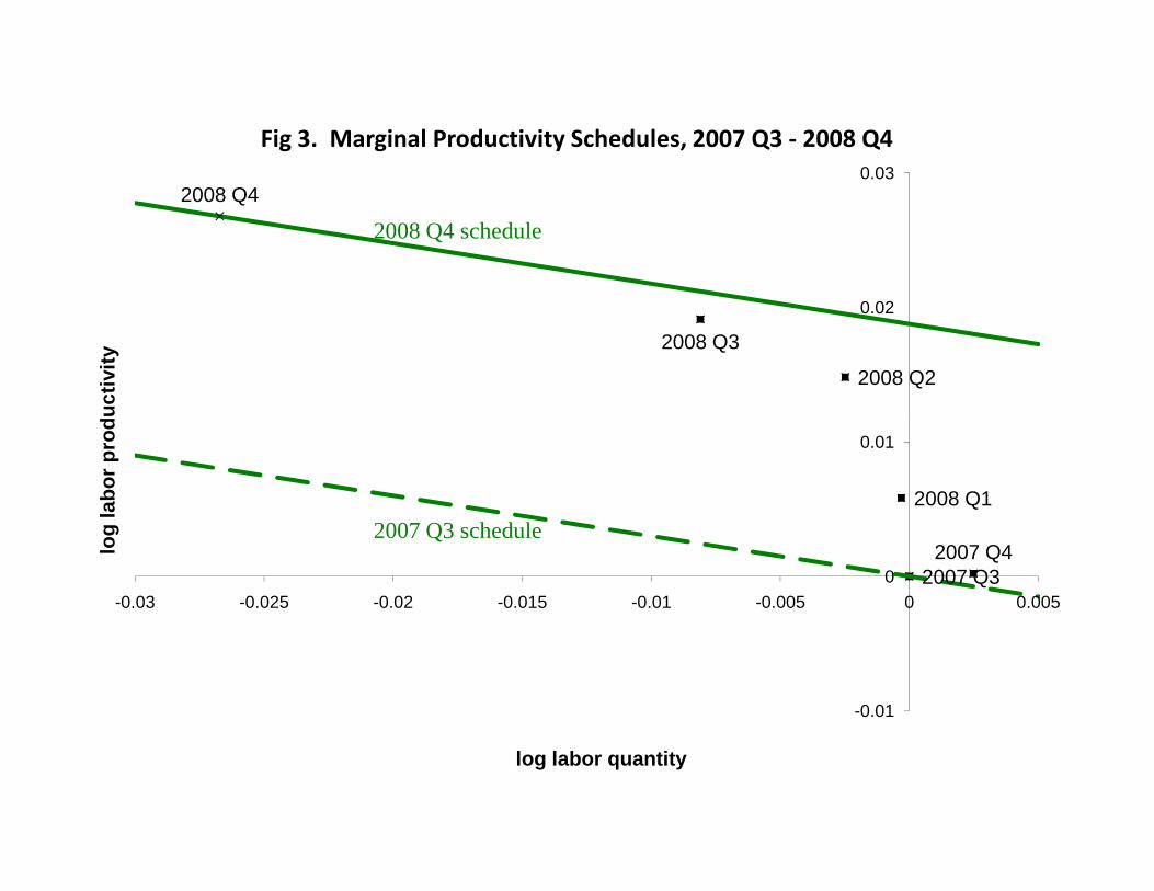
Figure 3 displays the calculation of the log of the residuals {At} for 2007 Q3

through 2008 Q4.3 Each date point in the Figure is the actual value of output per hour

and aggregate hours reported by the Bureau of Labor Statistics, measured on a

logarithmic scale with the origin normalized to be 2007 Q3. Two of the points have a

straight line (with slope -0.3) drawn through it representing the marginal productivity

schedule (1) applicable at that date. If (hypothetically), a single marginal productivity

schedule applied at each date, then all of the data points would be on the same straight

line with slope -0.3. In fact, each date is a different distance from any particular

schedule, so the log productivity residual measures the horizontal distance from the 2007

2 Recall that average and marginal productivity are proportional when production is Cobb-Douglas. 3 For the purposes of illustration, Oct-Nov 2008 productivity is assumed to be the same as 2008 Q3.

3

Q3 schedule and the actual data. Algebraically, the log residual is the inverse of the

definition (1).

ln ytln At ≡ ln nt + (2)0.3

To the extent that the schedule shown in Figure 3 is the aggregate marginal

productivity schedule, changes in A measure the amount by which the schedule shifted

over time. Since 2007 Q4, labor quantity has declined every quarter, and labor

productivity has risen. However, Figure 3 shows that, if the productivity schedule had

not shifted, labor productivity would have advanced only about one-third of what it

actually did.

Figure 4 displays the quarterly measures of log labor input nt and log residual At,

relative to their values for 2007 Q3. Labor input is changing much more over time than

is the residual. Under the marginal productivity interpretation of that residual, Figure 4

shows that most of the change in labor input over time is a change in labor supply or

labor market distortions rather than a shift in the marginal productivity schedule. When

viewed through the lens of any model in which aggregate output is a Cobb-Douglas

function of labor input with elasticity 0.7, aggregate adverse productivity shocks do not

seem to be an important impulse in this recession.

II.B. Marginal Productivity Shifts during Previous Recessions

Figures 5 and 6 display the change in the log productivity (ln yt) and log marginal

productivity residual (ln At) for the recessions of 1974, 1981, 1990, 2001, and 2008. For

each recession, the productivity residual is shown relative to its value in the quarter prior

to the NBER peak. Productivity normally increases in non-recession periods, although

the amount has varied from decade to decade. Productivity also increased in the 2001

and 2008 recessions. More notable are the earlier three recessions shown in Figure 5 in

which productivity declined (1970s and 1980s) or was pretty flat (1990s). As shown in

Figure 6, productivity failed to increase during the three earlier recessions because of

shifts of the marginal productivity schedule.

4

When viewed through the lens of a model in which aggregate output is a Cobb-

Douglas function of labor input with elasticity 0.7, aggregate productivity shocks do not

seem to be an important impulse in this recession or in the 2001 recession. But adverse

productivity shocks were part of the impulses of the three earlier recessions.

III.Neither Wealth nor Intertemporal Substitution Explains the “Supply” Shift

III.A. Consumption and Leisure have Moved in Opposite Directions

In theory, movements along the marginal productivity schedule can occur for a

variety of reasons: wealth effects, intertemporal substitution effects, preference changes,

and labor market distortions are among them. The wealth effect explanation says that

people work less because they feel richer. The intertemporal substitution effect says that

people work less in 2008 because they view 2008 as a relatively bad time to work and

produce income, either because the return to saving is low or because they expect future

labor productivity to be even higher than it is now. Both the wealth and substitution

effect theories imply that consumption is high during the recession (Barro and King,

1984).

Figure 2 easily rejects the wealth and intertemporal substitution effect

explanations because consumption expenditure has been low in this recession. In other

words, wealth and intertemporal substitution effects seem to be moving the economy

down the marginal productivity schedule, and the net result is less labor, so something

else must be moving the economy up the schedule even more.

III.B. A Labor Market Metric for Consumption Declines

Putting more structure on preferences for consumption and work permit me to

quantify the size of the wealth and intertemporal substitution effects, and thereby the size

of the leftward labor supply shift (or labor market distortion change) that would have

occurred absent those effects. In particular, I assume that the month t marginal rate of

substitution between consumption and leisure is proportional to the ratio of real

consumption per person to leisure time per adult:

5

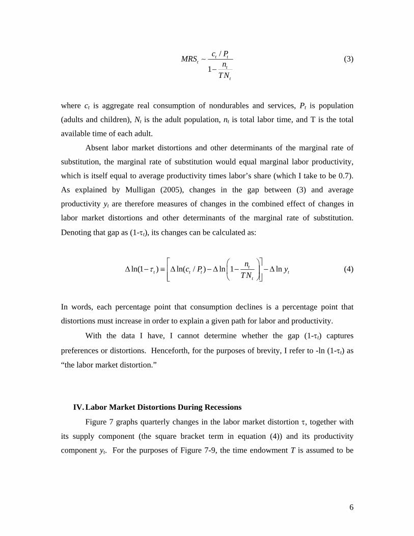
t /c PtMRSt ∼ (3)n1− t

TNt

where ct is aggregate real consumption of nondurables and services, Pt is population

(adults and children), Nt is the adult population, nt is total labor time, and T is the total

available time of each adult.

Absent labor market distortions and other determinants of the marginal rate of

substitution, the marginal rate of substitution would equal marginal labor productivity,

which is itself equal to average productivity times labor’s share (which I take to be 0.7).

As explained by Mulligan (2005), changes in the gap between (3) and average

productivity yt are therefore measures of changes in the combined effect of changes in

labor market distortions and other determinants of the marginal rate of substitution.

Denoting that gap as (1-τt), its changes can be calculated as:

⎡ ⎛ nt ⎞⎤≡ Δ⎢ t ⎜ ln yΔ ln(1 −τ t ) ln( c P/ t ) −Δ ln 1 − ⎟⎥ − Δ t (4)⎢ ⎝ TNt ⎠⎥⎦⎣

In words, each percentage point that consumption declines is a percentage point that

distortions must increase in order to explain a given path for labor and productivity.

With the data I have, I cannot determine whether the gap (1-τt) captures

preferences or distortions. Henceforth, for the purposes of brevity, I refer to -ln (1-τt) as

“the labor market distortion.”

IV. Labor Market Distortions During Recessions

Figure 7 graphs quarterly changes in the labor market distortion τ, together with

its supply component (the square bracket term in equation (4)) and its productivity

component yt. For the purposes of Figure 7-9, the time endowment T is assumed to be

6

four times the amount of labor per adult in 2002.4 Distortions increased throughout the

recession. Prior to 2008 Q2, much of the increase can described as stable consumption

and rising leisure in the face of rising productivity.5 From Q2 to Q4, productivity

continued to grow while consumption fell.

Figure 8 graphs quarterly changes in the MRS or “supply” term (the square

bracket term in equation (4)) for each of the recessions. The measured MRS falls in all of

the recessions, although little in 2001. The 2001 recession’s distinction in this regard

may not be a surprise given that productivity grew a lot in that recession. Figure 9 graphs

monthly MRS changes for the same recessions, showing how the MRS change for the

last six months of 2008 is one of the largest of all of the recessions.

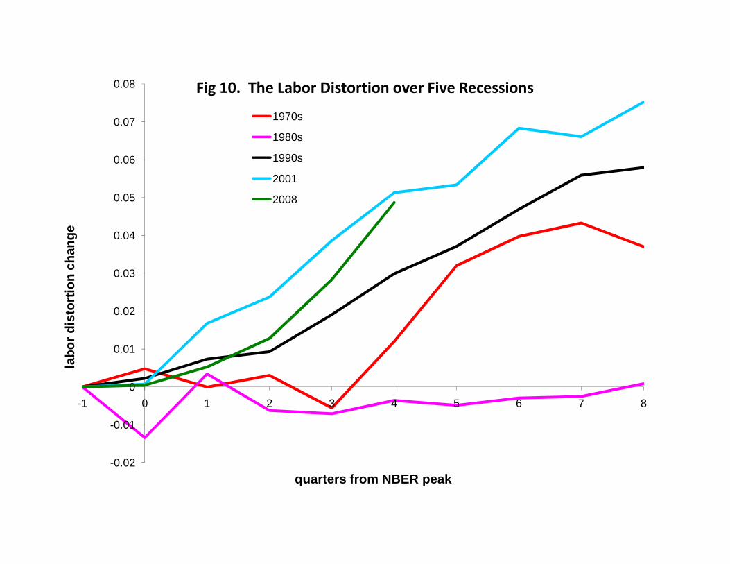
Figure 10 graphs quarterly changes in the labor market distortion τ for each of the

recessions. The 1970s and 1980s recessions had essentially no labor distortion change

through the first three quarters. Through four quarters, 2008 and 2001 recessions had the

largest changes of all of the recessions. The large MRS reduction through December

2008 in spite of the continued productivity growth is an expression of the key finding of

this paper: the employment decline is associated with a reduction in labor supply or an

increase in labor market distortions, rather than a reduction in the marginal product of

labor.

The labor demand equation (1) and the labor supply equation (4) can be used to

simulate the equilibrium labor and labor productivity if labor distortions and the labor

supply function had remained unchanged since the beginning of each recession yet

consumption, population, and the labor demand residual had followed their actual values.

For example, aggregate labor actually fell 0.027 log points 2007 Q3 through 2008 Q4

while the supply shift term ln (1-τ) fell 0.049 log points. If instead labor had risen 0.050

log points, the distortion term would have been constant over time and log average

productivity would have been essentially unchanged (specifically, 0.004 log points). In

other words, the labor supply distortion not only prevented an increase in labor that

4 2002 is the benchmark year for the BLS aggregrate hours index. 5 “Leisure” refers to adult time not spent working.

7

would have been consistent with the consumption drop, but actually reduced labor.6 In

this sense, the labor supply distortion is responsible for more than 100% of the

employment decline since December 2007.

V. Mortgage Modifications and Other Means-Tested Benefits: Possible Sources

of Reduced Labor Supply

Both labor and consumption have fallen in this recession even while productivity

rose. As shown in Figure 10, the labor distortion – or labor supply shift – apparently

emerging in the 2008 recession is on the order of five percentage points. What might

have caused the marginal rate of substitution to fall even while the marginal product was

rising?

One unique feature of this recession is that it was preceded by such a large

reduction in home prices. About 12 million homes are now worth less than the

mortgages owed on them. One way that mortgage lenders have responded to the loss in

the market value of mortgage collateral is to partially forgive borrowers with low

incomes.7 In 2008, the Federal Deposit Insurance Corporation (FDIC), Federal National

Mortgage Association (Fannie), and the Federal Home Loan Mortgage Corporation

(Freddie) all announced debt forgiveness or “loan modification” formulas. The FDIC’s

plan says “Modifications would be designed to achieve sustainable payments at a 38

percent debt-to-income ratio of principal, interest, taxes, and insurance.” (FDIC, 2008)

Several major mortgage servicers such as Bank of America, JPMorgan Chase and

Citigroup use those formulas for some of their delinquent borrowers. More recently,

mortgage modification has become available for “homeowners who make their mortgage

payments on time but who are struggling financially.”8

6 If 2008 Q4 real consumption per consumption per capita had been the same as in 2007 Q3, theproductivity residual followed its actual values, and the labor supply distortion had not changed over time, then log labor would have increased 0.035 log points. 7 Whether such forgiveness is in a bank’s unilateral interest, or encouraged by regulators, is a topic considered by Mulligan (2008). 8 http://www.usatoday.com/money/economy/housing/2008-12-11-foreclosures_N.htm

8

Much like banks use employment status and income as indicators for loan

qualification, banks use employment status and income as indicators of “struggling

financially.” For example, Citigroup and the U.S. Treasury announced November 24th:

“Citigroup will modify mortgages to help people avoid foreclosure along the lines of an FDIC plan that was put into effect at IndyMac Bank… struggling home borrowers pay interest rates of about three percent for five years. Rates are reduced so that borrowers aren't paying more than 38 percent of their pretax income on housing.” (Aversa, 2008)

Consider a family with a mortgage that is underwater in the amount b, and

anticipates the possibility of requesting mortgage modification early in 2009. The

mortgage is expected to be modified so that it pays a constant housing payment for the

years 2009-2014, after which time (for the purposes of illustration) the mortgage

payments will return to their initial contractual level. The annual amounts of the

payments for 2009-2014 are equal to 38 percent of 2008 family income, which the lender

verifies by reviewing the family’s 2008 tax return. Its budget constraint for leisure time

versus the present value of all other goods (future leisure, future consumption, and

current consumption) is shown in Figure 11. The point X is the amount of other goods

that would be affordable if the family had no income in 2008 but paid its mortgage in

full. At the point Y, the family is working enough, and thereby earning enough, that its

full mortgage payment is exactly 38% of its income. Points on the straight line through X

and Y are all possible choices for the family, assuming that they pay their mortgage in

full.

The point Z is b dollars above the point X, and is thereby the allocation available

to the family if it (a) defaulted on the mortgage, (b) did not earn income in 2008, and (c)

did not bear any foreclosure or moving costs. If the lender forgave the amount b without

conditions (and without foreclosure and moving costs), then the budget set would be

bound by the dashed black line, rather than the solid one. Mortgage modification with

the 38% formula offers the family the option of any of the allocations on the straight line

between Y and W. YW has slope equal to the slope of XY times (0.38R-1), where R is

the discount factor for a five year constant cash flow.9 YW slopes up because reducing

9 R is less than five, but likely greater than four. Thus, YW has a positive slope even though XY has a negative slope.

9

income by $1 in 2008 reduces bank payments by more than $1 in present value (namely,

$0.38 per year for five years).

For each dollar that 2008 income is reduced from what it would be at Y, the lender

is losing 0.38R compared to what it would get with full payment. As the choices along

YW get closer and closer to point W, the lender’s forgiveness approaches b. Once

forgiveness has reached b, the lender might as well foreclose rather than forgive any

more. Thus, the 38% formula implies that the family’s budget constraint includes

YWZX.10

Figure 11 is drawn for a relatively small value for b. However, if b were large

enough that point Z had more consumption than point Y, the budget constraint would

slope up over a wider range, as shown in Figure 12. In either case, there is a range of

incomes were income is effectively taxed at rates in excess of 100%. One does not have

to believe in elastic labor supply to strongly suspect that tax rates in excess of 100%

would change behavior. The only unknown right now is how many people were had

incomes in the relevant range and were aware of their modification opportunities.

Mortgage forgiveness is not the only work disincentive that has emerged during

this recession. The Internal Revenue Service announced that it would be lenient with tax

debts, but only for persons “struggling to pay their bills.” According to the Associated

Press (Ohlemacher, 2009),

“It's unrealistic to expect some taxpayers to make timely payments in this economy, [IRS Commissioner Doug] Shulman said. However, he cautioned that those seeking help will have to demonstrate their inability to pay.”

In other words, those who continue to earn will have to pay their taxes and IRS penalties

in full. Those who have reduced earnings will not.

It is possible that an “economic stimulus” law will pass the U.S. Congress. This

law may include tax breaks, spending plans, and further mortgage modification that

conditions those items on a person’s income (namely, those with low incomes will be

eligible for more help than those with high incomes). When all of the instances of

10 The lender may decide to foreclose before family income is as low as it is at W. In this case, some part of the triangle YWZ would be removed from the household’s budget set.

10

means-tests are considered in combination, a number of workers in the U.S. economy

may have a terrible incentive to work.

VI. Conclusions

Employment, hours, and consumption declined significantly in 2008, while labor

productivity rose. I decomposed these changes into three types of “causes”:

• productivity shocks that reduce labor and productivity,

• wealth and intertemporal substitution effects that reduce labor and raise

consumption, and

• (unmeasured) labor distortions and labor preferences that raise

productivity and reduce labor

It is well known (e.g., Barro and King, 1984; Hall, 1997) that previous business

cycles do not appear to be wealth or intertemporal substitution effects because both labor

and consumption decline. The 2008 recession is no different in this regard.

What is unique about the 2008 and 2001 recessions is the relative importance of

productivity and unmeasured labor distortions. Figures 13 and 14 are scatter plots

contrasting this recession and previous ones along these dimensions. Each recession is

one data point in the chart. The horizontal axis measures the change in the log

productivity residual from one quarter prior to the NBER peak to the second or fourth

quarter following the NBER peak (Figures 13 and 14, respectively). The vertical axis

measures the change in the unmeasured labor distortion (also in log points). The first

three recessions each had productivity shifts that were less than experienced during non-

recession years. The 2008 and 2001 recessions are unusual in that they have normal

productivity shifts throughout, but have adverse labor distortion shocks. The 1970s and

1980s had much less increase in the labor distortion than did the other recessions.

The Great Depression of the 1930s was unique in its magnitude, and therefore not

shown in Figures 13 and 14. Table 1 offers a comparison of the early 1930s to 2008. In

this recession, the productivity residual has increased. The productivity residual fell more

than 5 percent 1929-33 (Cole and Ohanian, 1999), which is many times more than it did

in the 1970s and 1980s recessions. The labor distortion increased many times more than

11

it did even in 2008 (Mulligan, 2005). Although it is not clear whether the Great

Depression was just an amplified version of the 1970s recession – with the labor

distortion rising and productivity residual falling – it is qualitatively different from the

2008 recession.11 The 2008 recession has not yet shown any adverse shift in the marginal

product of labor schedule.

Admittedly it is unclear whether and how public policy can “fix” a recession. But

even if we had a remedy for previous severe recessions, my finding that the 2008

recession is qualitatively different suggests that the proper remedy for this recession

would also be qualitatively different.

VII. References

Aversa, Jeannine. “Government Plans Massive Citigroup Rescue Effort.” Associated

Press. November 24, 2008.

Barro, Robert J. and Robert G. King. “Time Separable Preferences and Intertemporal

Substitution Models of Business Cycles.” Quarterly Journal of Economics.

99(4), November 1984: 817-39.

Chari, V. V., Patrick J. Kehoe, and Ellen R. McGrattan. “Business Cycle Accounting.”

Econometrica. 75(3), April 2007: 781-836.

Cole, Harold L. and Lee E. Ohanian. “The Great Depression in the United States from a

Neoclassical Perspective.” Federal Reserve Bank of Minneapolis Quarterly

Review. 23(1), Winter 1999: 2-24.

Cole, Harold L. and Lee E. Ohanian. “New Deal Policies and the Persistence of the

Great Depression: A General Equilibrium Analysis.” Journal of Political

Economy. 112(4), August 2004: 779-816.

Crucini, Mario J. and James Kahn. “Tariffs and Aggregate Economic Activity: Lessons

from the Great Depression.” Journal of Monetary Economics. 38(3), December

1996: 427-67.

11 Cole and Ohanian (1999, Table 6) find total factor productivity to fall five percent in the first year of the Great Depression, and a total of 14 percent through four years. Mulligan (2005, Figure 4) finds the Great Depression labor supply distortion to increase 0.17 log points in the first year and 0.46 log points through four years. In other words, 1929-30 would be in the same quadrant of Figure 15 as the 1970s recession, and on about the same ray from the origin, but five times further away.

12

Federal Deposit Insurance Corporation. “Loan Modification Program for Distressed

Indymac Mortgage Loans.” August 20, 2008.

http://www.fdic.gov/consumers/loans/modification/indymac.html

Friedman, Milton, and Schwartz, Anna J. A Monetary History of the United States,

1867–1960. Princeton, NJ: Princeton University Press (for NBER), 1963.

Gali, Jordi, Mark Gertler, and J. David Lopez-Salido. “Markups, Gaps, and the Welfare

Costs of Business Fluctuations.” manuscript, CREI, October 2003.

Hall, Robert E. “Macroeconomic Fluctuations and the Allocation of Time.” Journal of

Labor Economics. 15(1), Part 2 January 1997: S223-50.

Katz, Lawrence F. and Kevin M. Murphy. “Changes in Relative Wages, 1963-1987:

Supply and Demand Factors.” Quarterly Journal of Economics. 107(1),

February 1992: 35-78.

Kydland, Finn and Edward C. Prescott. “Time to Build and Aggregate Fluctuations.”

Econometrica. 50(6), November 1982: 1345-70.

Lucas, Robert E., Jr. “Bernanke is the Best Stimulus Right Now.” Wall Street Journal.

December 23, 2008.

Mulligan, Casey B. “A Century of Labor-Leisure Distortions.” NBER working paper no.

8774, February 2002.

Mulligan, Casey B. “Public Policies as Specification Errors.” Review of Economic Dynamics.

8(4), October 2005: 902-926.

Mulligan, Casey B. “A Depressing Scenario: Mortgage Debt Becomes Unemployment

Insurance.” NBER working paper no. 14514, November 2008.

Ohlemacher, Stephen. “IRS Agents Soften Heart for Delinquent Taxpayers.” January 6, 2009

(http://apnews.myway.com/article/20090106/D95HURKO1.html).

13

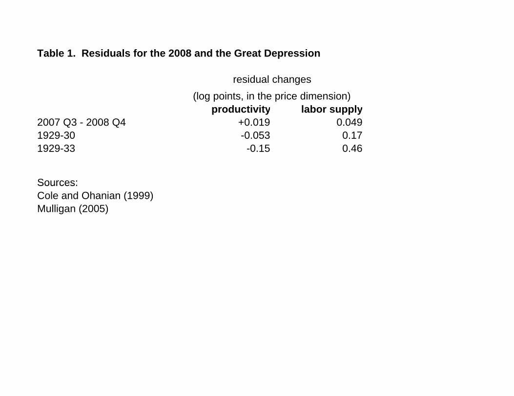
Table 1. Residuals for the 2008 and the Great Depression

residual changes(log points, in the price dimension)

productivity labor supply 2007 Q3 - 2008 Q4 +0.019 0.049 1929-30 -0.053 0.17 1929-33 -0.15 0.46

Sources:Sources:Cole and Ohanian (1999)Mulligan (2005)

              

   

     

           

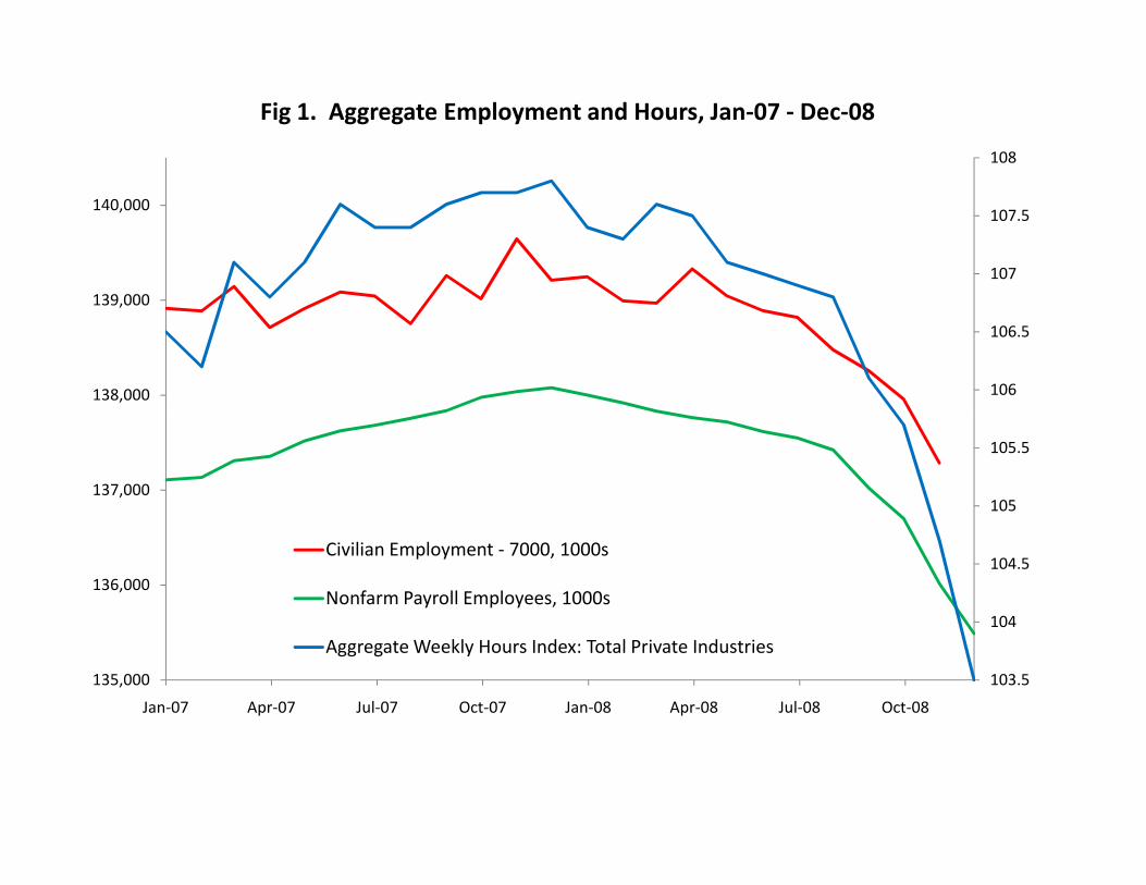
Fig 1. Aggregate Employment and Hours, Jan‐07 ‐ Dec‐08

106

106.5

107

107.5

108

138,000

139,000

140,000

103.5

104

104.5

105

105.5

135,000

136,000

137,000

Civilian Employment ‐ 7000, 1000s

Nonfarm Payroll Employees, 1000s

AggregateWeekly Hours Index: Total Private Industries

Jan‐07 Apr‐07 Jul‐07 Oct‐07 Jan‐08 Apr‐08 Jul‐08 Oct‐08

Fig 2. Real Per Capita Consumption, Jan-07 - Dec-08

0 060

-0.040

-0.020

0.000

0.020

Jan-07 Apr-07 Jul-07 Oct-07 Jan-08 Apr-08 Jul-08 Oct-08

m S

ep-0

7,

s &

pop

ulat

ion,

SA

(log change from Sep-07)

PCE - all

PCE - services

-0.160

-0.140

-0.120

-0.100

-0.080

-0.060

log

chan

ge fr

omde

flate

d by

PC

E de

flato

rs PCE services

PCE - nondurables

PCE - durables

Retail Sales

              

-0.03

2008 Q4

2008 Q4 schedule

0.02

2008 Q3

2008 Q2

0.01

2008 Q1 2007 Q3 schedule

2007 Q4 0 2007 Q3

-0.025 -0.02 -0.015 -0.01 -0.005 0

Fig 3. Marginal Productivity Schedules, 2007 Q3 ‐ 2008 Q40.03

-0.01

log

labo

r pro

d uct

ivity

log labor quantity

0.005

Fig 4. Labor and Productivity Residuals in the 2008 Recession

0.07

0.06 productivity residual labor

0.05

0.04

log

chaan

ge

0.03

0.02

0.01

0 2007Q3 2007Q4 2008Q1 2008Q2 2008Q3 2008Q4

-0.01

-0.02

-0.03

Fig 5. Productivity in 5 Recessions

0.04

0.05

0.06

0.07

0.08

ange

1970s

1980s

1990s

2001

2008

-0.03

-0.02

-0.01

0

0.01

0.02

0.03

-1 0 1 2 3 4 5 6 7 8log

prod

uctiv

ity c

ha

quarters from NBER peak

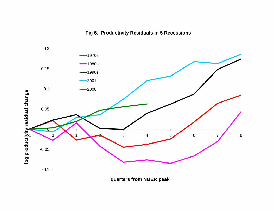
Fig 6. Productivity Residuals in 5 Recessions

0.1

0.15

0.2

ange

1970s

1980s

1990s

2001

2008

-0.1

-0.05

0

0.05

-1 0 1 2 3 4 5 6 7 8

log

prod

uctiv

ity re

sidu

al c

ha

quarters from NBER peak

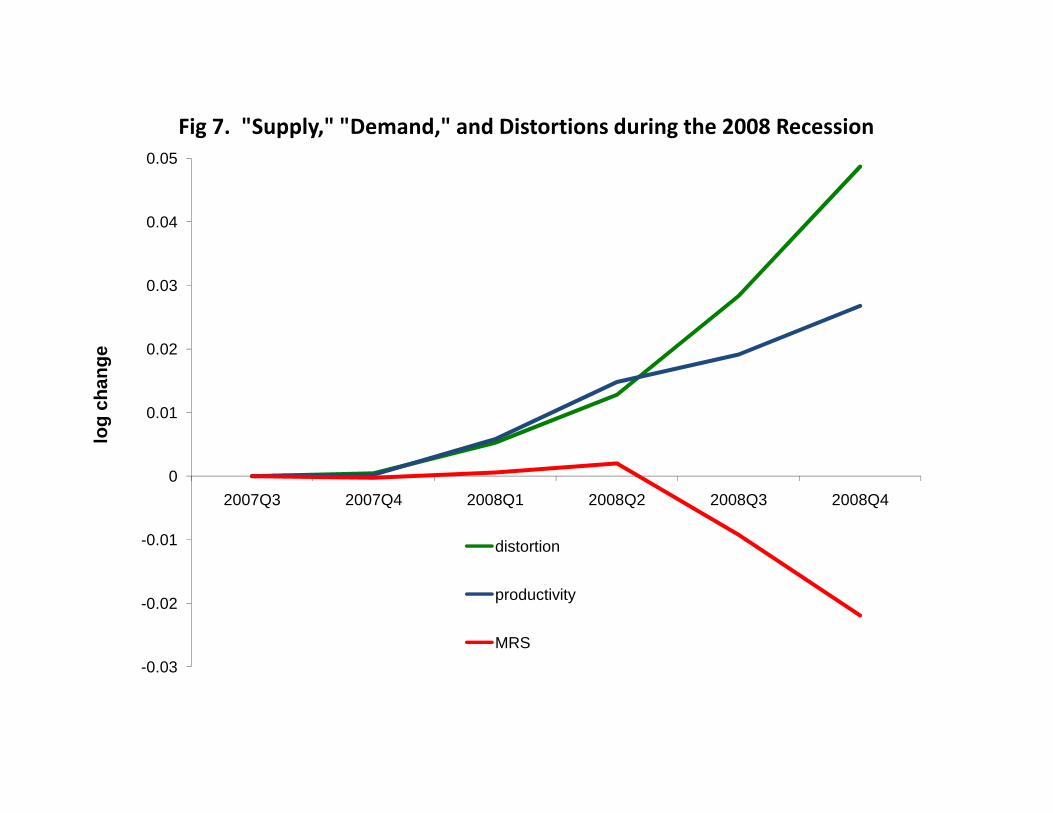
                  Fig 7. "Supply," "Demand," and Distortions during the 2008 Recession0.05

0.02

0.03

0.04

ange

-0.02

-0.01

0

0.01

2007Q3 2007Q4 2008Q1 2008Q2 2008Q3 2008Q4

log

cha

distortion

productivity

MRS-0.03

                    Fig 8. Quarterly Changes in the Consumption‐Leisure Ratio in FiveRecessions

0.01

0.02

0.03

ange

1970s

1980s

1990s

2001

2008

-0.03

-0.02

-0.01

0-1 0 1 2 3 4 5 6 7 8

log

MR

S ch

a

quarters from NBER peak

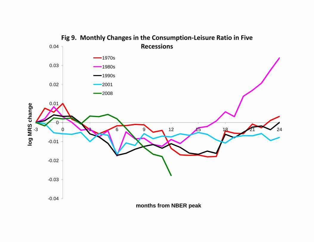
                    Fig 9. Monthly Changes in the Consumption‐Leisure Ratio in Five

0.01

0.02

0.03

0.04

ange

Recessions

1970s

1980s

1990s

2001

2008

-0.04

-0.03

-0.02

-0.01

0-3 0 3 6 9 12 15 18 21 24

log

MR

S ch

a

months from NBER peak

              

0.04

0.05

0.06

0.07

0.08ch

ange

Fig 10. The Labor Distortion over Five Recessions

1970s

1980s

1990s

2001

2008

-0.02

-0.01

0

0.01

0.02

0.03

-1 0 1 2 3 4 5 6 7 8

labo

r dis

tort

ion

c

quarters from NBER peak

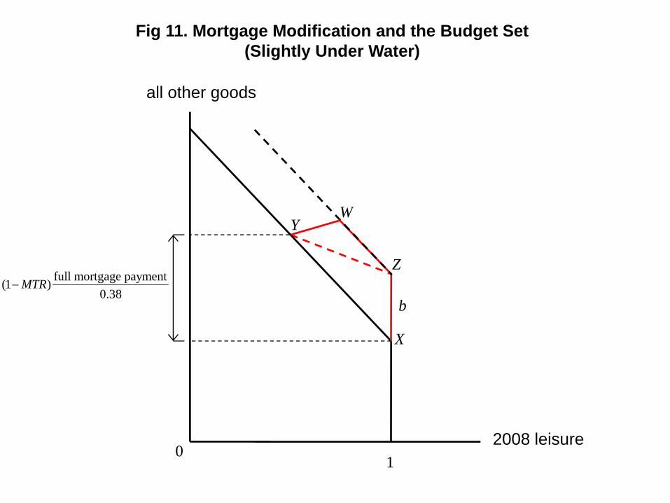
Fig 11. Mortgage Modification and the Budget Set (Slightly Under Water)

all other goods

WY

full mortgage payment (1−MTR) 0.38

b

X

Z

2008 leisure0

1

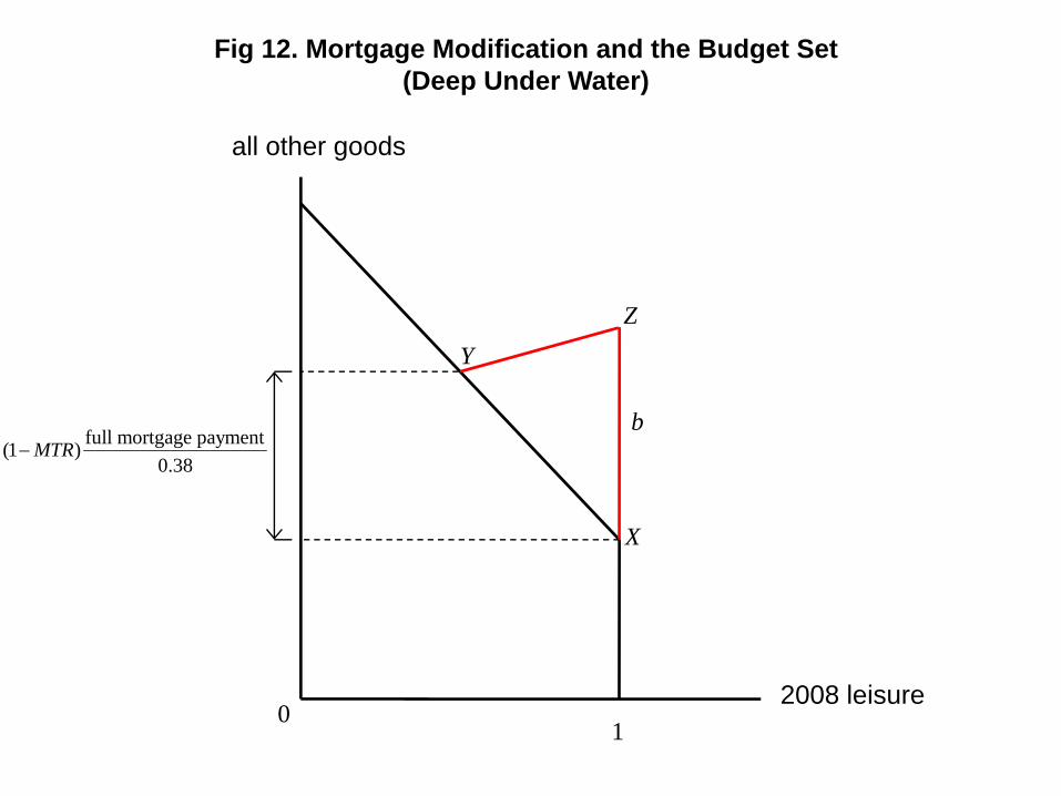
Fig 12. Mortgage Modification and the Budget Set (Deep Under Water)

all other goods

ZY

bfull mortgage payment (1−MTR)

0.38

X

2008 leisure0

1

                      

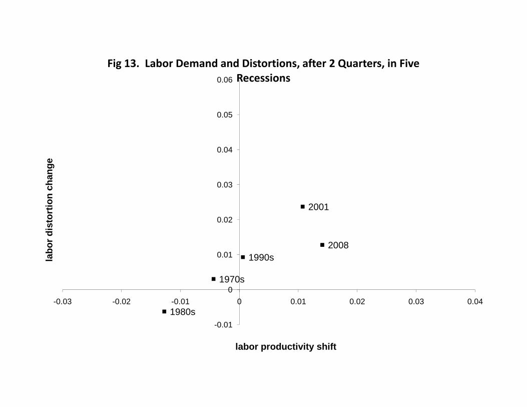
Fig 13. Labor Demand and Distortions, after 2 Quarters, in FiveRecessions

0.03

0.04

0.05

0.06

chan

ge

1970s

1980s

1990s

2001

2008

-0.01

0

0.01

0.02

-0.03 -0.02 -0.01 0 0.01 0.02 0.03 0.04

labo

r dis

tort

ion

c

labor productivity shift

                      

Fig 14. Labor Demand and Distortions, after 4 Quarters, in Five

1990s

20012008

0.03

0.04

0.05

0.06

chan

ge

Recessions

1970s

1980s

-0.01

0

0.01

0.02

-0.03 -0.02 -0.01 0 0.01 0.02 0.03 0.04

labo

r dis

tort

ion

c

labor productivity shift