Case Study – Multi-Modal Reconfigurable Processing Unit

Prof. Dr. Christian Plessl

SS 2017

High-Performance IT Systems groupPaderborn University

Version 1.5.0 – 2017-07-14

Outline

• modern parallel computer architectures– CPUs + emerging parallel architectures– reconfigurable computing– challenges for high-performance computing

• high-level performance estimation for reconfigurable computers– motivation– approach and results

• conclusion

2

Advantages of general-purpose CPUs

• programmability– widely known and mature programming languages– simple programming models (sequential model for most languages)– mature optimizing compilers

• wide applicability– general purpose CPUs are designed for a wide range of applications– programmers don’t need to consider CPU architecture details– many libraries available (numerics, image processing, cryptography, ...)– binary compatibility among CPUs of the same family

• inexpensive– commodity product, economy of scale

• tremendous performance growth– driven by progress in semiconductor technology– no change of software required– this "free lunch" promise pushed alternative computer architectures into a

niche

3

Inefficiencies of a general-purpose CPUs

• not tailored to particular task– unknown applications– unknown program flow– unknown memory access patterns– unknown parallelism

• generality causes inefficiencies– poor relation of active chip area to

total area– excessive power consumption– difficult design process

• multi-core CPUs try to sustain the progress of the general purpose CPUs

4

die shot of a 4-core AMD Barcelona CPU

chip area that contributes toactual computation

source: Anandtech

Stagnation in single-core CPU performance

• single-core CPU performance stagnates since ~2005– power dissipation of a processor is limited to ~150W– shift from few fast CPU cores to many efficient, but slower cores– increasing performance now requires parallel computing!

5Figure: Chuck Moore, AMD Technology Group CTO

Data Processing in Exascale-class Computing Systems | April 27, 2011 | CRM 3

Transistors (thousands) Single-thread Performance (SpecINT) Frequency (MHz) Typical Power (Watts) Number of Cores

Original data collected and plotted by M. Horowitz, F. Labonte, O. Shacham, K. Olukotun, L. Hammond and C. Batten Dotted line extrapolations by C. Moore

35 YEARS OF MICROPROCESSOR TREND DATA

Scaling up performance through parallelism

• exploit parallelism on many levels– core-level: vector instructions, multiple issue– chip-level: multi-cores– server-level: several CPUs per server– data center-level: many servers with fast interconnect

• objectives– improve performance by spreading work to many processors– improve energy efficiency by using processors optimized for efficiency

instead of single core performance

• challenges– parallelizing applications is generally a difficult problem– poor development tool support

6

application

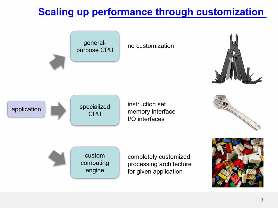
Scaling up performance through customization

general-purpose CPU

no customization

specialized CPU

instruction setmemory interfaceI/O interfaces

custom computing

engine

completely customized processing architecture for given application

7

Example for a custom computing engine

• bioinformatics (data mining): search in genome sequences

DNA sequence data

G A T C

=

&

'A'

A

=

'T'

A

=

'C'

=

'A'

match'A'

match'T'

match'C'

match'A'

match 'ATCA'

no

DNA sequence data

G A T C A

=

&

'A'

A

=

'T'

-

=

'C'

=

'A'

match'A'

match'T'

match'C'

match'A'

match 'ATCA'

no

DNA sequence data

G A T C A A -

=

&

'A'

-

=

'T'

-

=

'C'

=

'A'

match'A'

match'T'

match'C'

match'A'

match 'ATCA'

no

G

DNA sequence data

A T C A A - -

=

&

'A'

-

=

'T'

-

=

'C'

=

'A'

match'A'

match'T'

match'C'

match'A'

match 'ATCA'

no

DNA sequence data

G A T C A A

=

&

'A'

-

=

'T'

-

=

'C'

=

'A'

match'A'

match'T'

match'C'

match'A'

match 'ATCA'

no

DNA sequence data

G A T

=

&

'A'

C

=

'T'

A

=

'C'

=

'A'

match'A'

match'T'

match'C'

match'A'

match 'ATCA'

yes

application-specificinterconnect

data stream computingand pipelining

customoperations

paralleloperations

wide data paths

custom datatypes

8

Custom computing technology

• field programmable gate array (FPGA)– software programmable configurable

logic blocks– software programmable interconnect– massively parallel

• can implement any custom computing engine– typically 5-100x improvement in

performance or energy over single core CPU

– domains: bioinformatics, pattern matching, financial computation, molecular dynamics, ...

9

X

X

X

X

X

X

X X X

configurableboolean logic

flipflop

Reconfigurable computing systems

• experimental academic systems– proof-of-concept demonstrators

• PCI-attached FPGA acceleration cards– most widely spread platforms

• integrated FPGA solutions for HPC– tight integration of CPU and FPGAs– access to shared system memory– target market: HPC

10

eg. Sundance, Alpha Data, Nallatech, ...

TKDM, in-house development at ETH

Convey HC-1 hybrid core computer

Challenges for high-performance RC

• high speedups for many interesting applications have been demonstrated– combinatorial optimization (minimum covering, cube cut): >100x speedup– digital signal processing (filtering): 10x speedup– k-th nearest neighbor method: 74x speedup

• but reconfigurable computing is still not widely used in HPC

• challenges for a widespread adoption– programming is difficult: expert knowledge in application domain and

circuit design required– unstructured design process: many complex system-level decisions are

made ad-hoc (system architecture, accelerator architecture, hw/swpartitioning)

– missing performance models: performance known only after implementation

11

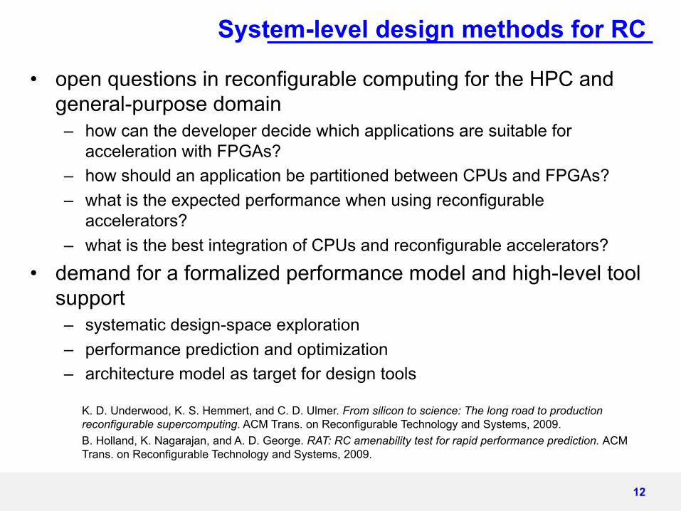
System-level design methods for RC

• open questions in reconfigurable computing for the HPC and general-purpose domain– how can the developer decide which applications are suitable for

acceleration with FPGAs?– how should an application be partitioned between CPUs and FPGAs?– what is the expected performance when using reconfigurable

accelerators?– what is the best integration of CPUs and reconfigurable accelerators?

• demand for a formalized performance model and high-level tool support– systematic design-space exploration– performance prediction and optimization– architecture model as target for design tools

K. D. Underwood, K. S. Hemmert, and C. D. Ulmer. From silicon to science: The long road to production reconfigurable supercomputing. ACM Trans. on Reconfigurable Technology and Systems, 2009.B. Holland, K. Nagarajan, and A. D. George. RAT: RC amenability test for rapid performance prediction. ACM Trans. on Reconfigurable Technology and Systems, 2009.

12

Performance Modeling for CPU/Accelerator Architectures

• estimate performance of applications when mapped to CPU/accelerator architectures– high level of abstraction– determine which application parts shall

be moved to the accelerator– determine performance with analytical

model

13

CPU ReconfigurableAccelerator

Control

Register

Private L1

Shared L2

Private L1 or Local Memory

Main Memory

exemplary CPU/accelerator architecture with shared L2 cache

S. A. Spacey, W. Luk, P. H. J. Kelly, and D. Kuhn. Rapid design space visualization through hardware/software partitioning. In Proc. Southern Programmable Logic Conference. 2009.

control-flow graph of an application

? ?

?

High-level performance estimation framework

• co-simulation: usual approach for evaluation of reconfigurable computer architectures– provides accurate results for one design point– time consuming design process of simulator– often manual mapping of application

• main problem: mutual dependency of– interface parameters– granularity of tasks in hardware/software partitioning– achievable speedups

• our approach: high-level estimation– focus on system-level aspect, model accelerator at a high-level of

abstraction– fully automated study of architecture parameters– determining the acceleration potential for a broad range of applications

14

Performance estimation tool flow

• operates in two stages• 1. application characterization

– compilation of benchmark with LLVM compiler framework

– static code analysis: control data flow graphs, define/use of values

– dynamic code analysis gathered with profiling: data dependencies, control flow

– cache simulation• 2. hardware/software partitioning

– assign basic blocks to CPU or accelerator

– iterative greedy partitioner (2 variants)

– optimal partitioning with integer linear programming

15

compile application to LLVM

profile with benchmark input data• execution counts of basic blocks• control flows• data flows and cache access

application characterization

once

per

ben

chm

ark

Perform Estimation

Move Basic Blocks

start with initial partitioning (all blocks mapped to CPU)

partitioning and performance estimation once

/iter

ativ

e de

pend

ing

on m

etho

d

Architecture Parameters

CPU ReconfigurableAccelerator

Control

Register

Private L1

Shared L2

Private L1 or Local Memory

Main Memory

Application and architecture characterization

• static application properties– instructions– basic blocks– variables (registers)

used/written

• dynamic application properties– execution counts– number of control flows– cache level serving

memory operation

• architecture parameters– execution efficiency– control transfer latency– memory access latency– register transfer latency– capacity

• partitioning– mapping of basic block

€

I = {I1,I2,…,Inins}

€

B = {B1,B2,…,Bnblks}

€

Ru(Bl )

€

Rw (Bl )

€

n(Ik )

€

n(Bl )

€

n(Bl ,Bm )

€

v(Ikj )

€

p(Bl ) = {CPU,ACC}

CPI(CPU) CPI(ACC)

€

λm (L1)

€

λm (L2)

€

λm (MEM)

€

λc

€

λr,push

€

λr,pull

€

σ(ACC)

16

CPU ReconfigurableAccelerator

Control

Register

Private L1

Shared L2

Private L1 or Local Memory

Main Memory

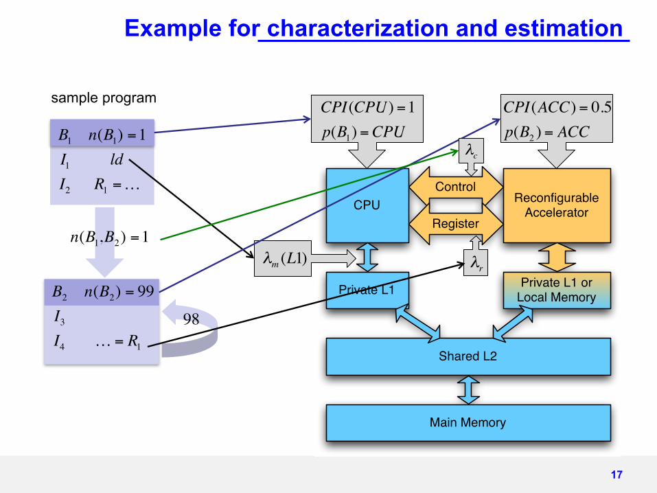
Example for characterization and estimation

sample program CPI(CPU) =1p(B1) =CPU

CPI(ACC) = 0.5p(B2 ) = ACC

€

λm (L1)

€

λr

€

n(B1,B2) =1

€

B1 n(B1) =1I1 ldI2 R1 =…

€

B2 n(B2) = 99I3I4 … = R1

€

98

λc

17

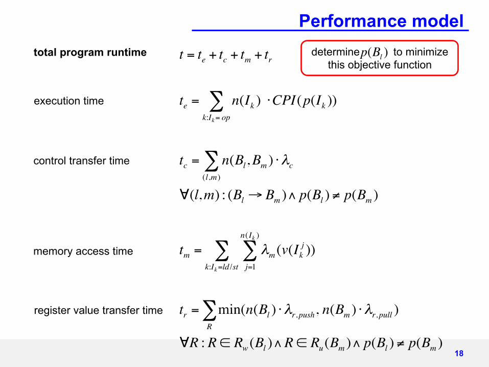
Performance model

t = te + tc + tm + tr

te = n(Ik ) ⋅CPI(p(Ik ))k:Ik= op∑

tc = n(Bl,Bm ) ⋅λc(l,m)∑

∀(l,m) : (Bl → Bm )∧ p(Bl ) ≠ p(Bm )

tm = λm (v(Ikj )

j=1

n(Ik )

∑k:Ik=ld /st∑ )

tr = min(n(Bl ) ⋅λr,push, n(Bm ) ⋅λr,pull )R∑

∀R :R ∈ Rw (Bl )∧R ∈ Ru(Bm )∧ p(Bl ) ≠ p(Bm )

total program runtime

execution time

memory access time

control transfer time

register value transfer time

determine to minimize this objective function

p(Bl )

18

Experimental setup (1)

• framework implemented in C++– leverages and extends LLVM compiler infrastructure– custom cache simulator

• speed of the tool flow– application characterization: ~15 minutes (for all benchmarks)– partitioning: ~10 seconds (for all benchmarks)– measured on MacBook Pro, Intel Core2 Duo 2.2 GHz

• greedy hardware/software partitioner– block level: consider individual basic blocks as partitioning objects– multi level: consider blocks, loops, loop-nets, and functions as

partitioning objects– select object with best speedup/size ratio

19

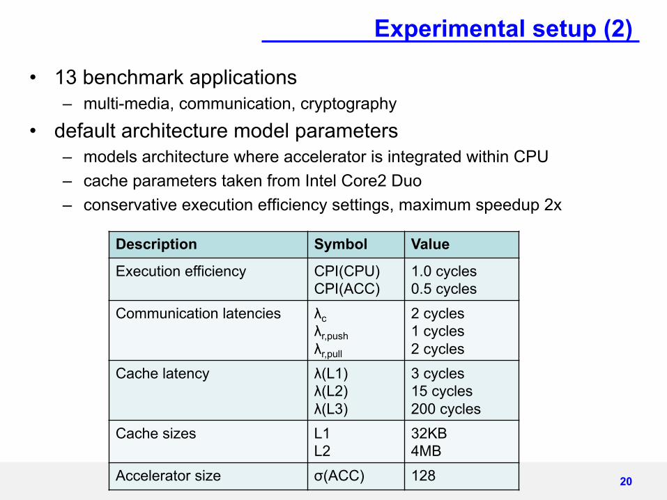
Experimental setup (2)

• 13 benchmark applications– multi-media, communication, cryptography

• default architecture model parameters– models architecture where accelerator is integrated within CPU– cache parameters taken from Intel Core2 Duo– conservative execution efficiency settings, maximum speedup 2x

20

Description Symbol Value

Execution efficiency CPI(CPU)CPI(ACC)

1.0 cycles0.5 cycles

Communication latencies λcλr,pushλr,pull

2 cycles1 cycles2 cycles

Cache latency λ(L1)λ(L2)λ(L3)

3 cycles15 cycles200 cycles

Cache sizes L1L2

32KB4MB

Accelerator size σ(ACC) 128

Visualization of multilevel partitioning

application: ADPCM

basic blocks, border width proportional log(execution time)control flows, border width proportional log(communication time)

21

What accelerator size should be provided?

• conclusions– distinct threshold behavior (whole kernel must fit to exploit performance)– modest accelerator sizes will be sufficient

1 1.05

1.1 1.15

1.2 1.25

1.3 1.35

1.4 1.45

2 4 8 16 32 64 128 256 512 1024 2048

Spee

dup

Accelerator size

AVG13StringWhet

FFTSHABlow

MD5JPEG

22

Which memory level should be shared?

• conclusions– a local memory for the accelerator is mandatory (cache or scratchpad)– latency penalty for shared caches has a large impact for L1

1 1.05 1.1

1.15 1.2

1.25 1.3

1.35

SL1 SL2+ SL2- SMM+ SMM-

Spee

dup

Cache configuration

AVG w/o pen.AVG with pen.

SL1 CPU/ACC share data via L1 cacheSL2+ CPU/ACC share data via L2 cache, ACC has local L1 memorySL2- CPU/ACC share data via L2 cache, ACC has no local L1 memorySMM+ CPU/ACC share data via main memory, ACC has local L1 memorySMM- CPU/ACC share data via main memory, ACC has no local L1 memory

23

How important is the partitioner heuristic?

• conclusions– the multi level greedy partitioner is clearly superior– the impact of the heuristic depends strongly on the application

1 1.1 1.2 1.3 1.4 1.5 1.6 1.7 1.8 1.9

2

AESBlowfish

MD5SHA

JPEGFFT

SORWhetstone

ADPCM

CRC32

Dijkstra

StringSusan

Spee

dup

Benchmark

Block levelMulti level

24

How important is a low latency of the interface?

• conclusions– when using block level partitioning a low latency interface is important– for multi level partitioning longer latencies can be tolerated

1 1.05 1.1

1.15 1.2

1.25 1.3

1.35 1.4

0.25 0.5 1 2 4 8 16 32 64 128 256 512

Spee

dup

Latency factor compared to default setting

Block levelMulti level

25

Further reading

• publication– T. Kenter, M. Platzner, C. Plessl, and M. Kauschke. Performance estimation for the exploration

of CPU-accelerator architectures. Proc. Workshop on Architectural Research Prototyping, 2010.– T. Kenter, M. Platzner, C. Plessl, and M. Kauschke. Performance estimation framework for

automated exploration of CPU-accelerator architectures. Proc. Int. Symp. on Field-Programmable Gate Arrays (FPGA), 2011.

26

Changes

• 2017-07-14 (v1.4.0)– updated for SS 2017

• 2014-07-17 (v1.3.1)– minor updates to introduction

• 2014-06-26 (v1.3.0)– updated for SS 2014

• 2013-07-17 (v1.2.0)– updated for SS 2013

• 2012-07-12 (v1.1.1)– update to animations and some introductory slides

• 2012-06-15 (v1.1.0)– updated for SS 2012

• 2011-06-30 (v1.0.0)– initial version

27