Embed Size (px)
Citation preview
Cars, Radios & Store SizeRetailing in the Early 20th Century
Todd C. NeumannUniversity of Arizona
Friday, July 1, 2005
Abstract
This paper examines the endogenous number of retail establishments across a widevariety of segments and markets in order to determine the nature of competition inthe retail industry during the early 20th century. Using data from the first Census ofRetail Distribution in a discrete dependent variable model I find many of the retailsegments studied operated in a competitive environment in 1929. Special attentionis given to how the spread of the automobile, changes in female labor forceparticipation, the geographic size of a city, and the spread of mass marketingaffected the value of the services provided by retailers and in turn entry thresholds.Evidence suggests variation in some of these factors played a role in determining thevalue of retail services and the level of competition in a market. Furthermore,exogenous changes in these factors might explain increasing store size through time.
Preliminary Draft. Please do not cite or distribute without authors’ consent.
I. Introduction
Today there is no shortage of press on how Wal-Mart™ and other “big box” stores are destroying the
small retailer. However, concern over the future of “mom & pop” stores is not a recent phenomenon. Early in the
20th century it became obvious that stores were growing larger, although how large they would grow was difficult
to predict. Lawrence Mann wrote in the AER. in 1923, “Their (small stores) relative importance will probably
continue to decrease, but there is no probability that they will all be forced out of business, as they usually have the
2
advantage of convenience of location…and give more personal service.” As time progressed fewer people were as
confident as Mann. A nationwide census of retail stores in 1929 provided the first empirical evidence of how the
country’s retail segment was changing. That data allows one to explore the beginnings of what we are witnessing
today and what concerned many over 75 years ago.
Using data from the 1930 Census of Retail Trade this paper will provide insight on two important retail
issues of the early 20th century. The first is exactly how competitive retailers were in the first part of the 20th
century. Many at the time suggested that the lack of a strong competitive climate resulted in small and inefficient
retail stores that earned above normal profits. Meanwhile evidence gathered that retail store size was growing–the
beginning of the Wal-Mart™ phenomenon. I will attempt to identify factors that may have caused this increase in
size and might explain the further increases in store size or entry threshold that have been observed throughout
the 20th century. I will start by describing some of the economic literature dealing with American retailing.
Generally this is divided into early reduced form empirical studies that first used the data gathered from the
various Business Censuses to provide descriptive pictures of the industry; and more recent work, which began to
explore theoretical and empirical factors that contribute to changes in the size and structure of retailers. The early
papers tended to focus on questions of efficiency without providing a clear conceptual framework of retailing. On
the other hand, the few recent studies often provide more narrow frameworks particular to a type of retailer or
situation. After summarizing some of these I will lay out a broader framework that can be used to think about the
fundamentals of retailing. Namely, I explore what exactly it is that retailers produce; where demand comes from
for this product; how retailers produce this product; and what demand and supply conditions may change to alter
the structure of retailers. Using this background I define a simple profit function of a retailer that can be used to
estimate population entry thresholds for a market. Note, the population entry threshold or the number of people
required to support a certain number of retail stores in a market is analogous to retail store size. I will give special
attention to factors that may explain variation in these entry thresholds across markets. Finally using 1929 data
from the Retail Census I estimate these thresholds and use them to infer the competitive nature of retailers and
how specifically the introduction of the automobile and new mass marketing mediums altered the competitive
conduct and size of stores.

3
A Changing Industry
Like manufacturing and agriculture, retail distribution changed dramatically over the course of the 20th
century. This change is evident in Table 1. For example, in 2002 a total of 2,055,500 retail stores were open,
1,059,328 with paid employees1. This amounted to approximately 7.1 stores per 1000 people or less than 4 stores
with payroll per thousand. Conversely in 1929 there was a total of 12.6 stores per thousand people and over 7
stores with employees per thousand. A clear and dramatic decline has occurred in the number of retail stores per
capita. At the same time the size of stores as measured by sales has increased significantly. Between 1929 and
2002 the average size of a store with employees rose over 437 percent. These changes coincided with a relative
shift away from labor utilization in the production of retail service. While the average gross margin was the same in
1929 and 2002, labor expenses as a share of that margin have dropped nearly in half. At the same time the number
of employees per dollar sold has fallen over 60%. These figures indicate a number of things. First entry thresholds
for retailers have increased significantly. Second, relatively fewer employees are being used today to produce
drastically more retail service output. This suggests that retail workers are vastly more productive today and/or
that retailers are using other inputs to create retail output. Finally, despite the increase in labor productivity and
larger (some might presume more efficient) stores the gross margin has not changed.
Table 1Characteristics of Retail Stores in 1929 and 2002
1929 2002
All Stores
Storeswith
Employees All Stores
Storeswith
EmployeesNumber of Establishments 1,543,214 885,8042 2,055,500 1,059,328
Sales as % of total NA 90.1%1 NA 98.0%Stores per 1000 people 12.6 7.21 7.1 3.7
Average Sales per store (2002$) $334,466 $525,007 $1,490,300 $2,824,200Gross Margin 28% NA 28% NA
Labor as share of Gross Margin NA 57% NA 33%Employees per $100,000 Sales (2002$) 1.17 1.29 .49 .50
Employees per Store 3.9 6.8 7.3 14.2Source: 15th Census of the United States & 2002 Census of American Business and Annual Survey of Retail Trade
A changing industry alone need not necessitate inquiry. However, unlike the more extensively studied
manufacturing and agriculture industries, the structural changes in retailing coincide with the growing importance
of the industry as measured by sales and employment. In 2002, retail sales accounted for over 43% of personal
1 Excluding non-store retailers2 Based on share from 1939 Census
4
consumption expenditures3. Today retail employment is growing and approaching nearly 18% of the American
workforce, while manufacturing employment is at 14% and falling4.
The changes evident from Table 1 were well underway by the time the first retail census was conducted.
Anecdotally economists and entrepreneurs alike recognized that retail establishment size and firm organization
were changing. Small, family run enterprises were being replaced by larger stores, often with chain affiliations.
During the same period the general operation of retail establishments was undergoing transformation. Until this
time, a customer was attended to individually in most retail stores. This included grocery, dry goods, and apparel
stores (among others) where a customer would request an item and have it delivered from storage5. This labor-
intensive mode, however, was quickly being replaced by the self-service models that we are familiar with today.
The changes occurring within the store coincided with significant changes in the broader economy.
Industrialization, mass marketing of consumer goods, greater female labor force participation, and the spread of
the automobile all occurred in the first 30 years of the 20th century. These socioeconomic changes renewed debate
about the efficiency and competitiveness of retailing. Concern was grounded in what many believed to be
unjustifiably large gross margins. Mann (1923) notes persistent statements that “the chief waste in delivering
goods to the ultimate consumer is due to ‘middlemen’ and that the ‘middlemen’ obtain exorbitant profits.” Even
with large selections of retailers from which to choose, these margins lead many to conclude that the industry was
not competitive either because of collusion, product differentiation, or some combination of the two.6
Despite all this upheaval, economists were ill equipped to analyze the industry due to a lack of
comprehensive data7. The 15th Census of the United States and its new section devoted to Retail Distribution
provided the first dataset of retail patterns across the country.
Empirical Technique
Until recently the traditional method of exploring the competitive nature of an industry was the structure-
conduct-performance paradigm. These methods used by Bain (1956), among others, looked at the correlation
between measures of market structure (such as concentration) and market performance (such as price cost ratios).
While these methods offered intuitive appeal they suffered from a number of criticisms, most notably the ad hoc
3 Bureau of Economic Analysis (www.bea.gov)4 Bureau of Labor Statistics (www.bls.gov)5 Bucklin (1972) pg. 856 Bucklin (1972) pg. 1157 Mann (1923)
5
assumption on the direction of causality from structure to conduct to performance. In reality an observed market
structure is a function of the performance and conduct of the existing profit maximizing firms. Equilibrium
structure, conduct, and performance are determined by profit maximizing agents reacting to the actual number of
market participants, potential entrants, and other exogenous factors of the market, which may affect demand or
costs.
New empirical techniques have been developed to address this fundamental endogeneity between
structure, conduct, and performance. One of them has been the use of discrete dependent variable models by
Bresnahan and Reiss (1990) and Berry (1992) to estimate the underlying profit maximizing decisions of firms. In
these models firms enter a market if post equilibrium profits will be positive. Using market data on firm counts
and the nature or size of the market, one can use discrete choice models to estimate parameters of the underlying
profit function. Various papers by Reiss and Spiller (1989), Bresnahan & Reiss (1991b), Stavins (1995), Downes
and Greenstein (1996), Berry and Waldfogel (1999), Mazzeo (1999), Abraham et al. (2000), and Manuszak (2002)
have used this approach to explore the structure of markets in different industries. Bresnahan and Reiss (1991b)
look at entry thresholds in retail and professional markets using contemporary data. Lacking information on price-
cost margins, they develop tests based on estimates of entry thresholds that can shed light on the market size
required to support entry. These techniques offer information on the competitive nature of the industry in a given
market by comparing breakeven market sizes. A market with 2 stores should require twice the population of a
market with 1 store. However, if the duopoly threshold is greater than twice that of the monopoly market it
suggests the monopolist is exercising market power, pricing above average cost, and this mark up is reduced by
the entry of a second store. Meanwhile if one observes that the population per store is similar between markets
with 3 and 4 stores, one can presume competition has driven price down to average cost by the time a market has
3 stores.
This paper employs the methods developed by Bresnahan and Reiss (1991b) to provide insight on two of
the major issues described above: the competitive/efficient nature of retailing in 1929; and the apparent increase in
store size or entry threshold as it relates to broader socioeconomic changes that began in the first 3 decades of the
century and continued through much of the rest. Like their study I use counts of retail establishments to infer the
competitiveness of each retail segment examined in 1929. A competitive industry in turn can be assumed to be
relatively efficient as competitive pressures will drive stores to produce in the most optimal way. I will also
examine more closely factors that affected the competitive nature of a retail market. Of particular interest is how
6
the spread of the automobile and new mass marketing mediums altered the competitive conduct of stores. The
primary source of data is the 19308 15th Census of the United States, Retail Distribution Section. It was the first
comprehensive attempt to gather data on the industry and later evolved into the bi-decade Census of Business
conducted today by the United States Census Bureau. This information is augmented with data from various other
historical sources in an attempt to gather further information about the markets studied in this paper.
In general I find that many of the retail segments examined appeared to be competitive in 1929. In other
words for the typical market, entry by a subsequent store would not change significantly per store entry
thresholds. In the process of estimating these thresholds I find factors beyond population that affected the
demand for retail services as well as factors that may have increased or decreased the effect of entry. Female labor
force participation is associated with higher variable profits; radio ownership seems to have reduced the effect of
entry on variable profits; and automobile ownership is associated with larger entry thresholds.
II. Literature Review
Early Studies of Retailing
Lawrence Mann wrote in his 1923 AER essay, The Importance of Retail Trade in the United States, “No
important field of business statistics has been so neglected by both governmental and private investigators as that
of retail.” His piece began and attempted to encourage further study by laying out the size of the industry in terms
of employment and sales. Mann notes that in 1919 retailing ranked as the country’s third largest industry. His
Federal Reserve Bank data confirmed what many had been anecdotally observing since the turn of the century.
Total retail sales were rising at the same time that the number of retail establishments was remaining steady or
falling. Consequently, by 1923 it was apparent that the size of retail establishments was increasing rapidly. In other
words, entry thresholds were rising.
Following the first Census of Retail Trade in 1930 more empirical attention was given to the industry.
Whiteley (1936) makes a cross-country comparison between the retail situations in Canada and the United States.
He finds that the two are remarkably similar in the make up of store type, size, cost structure, employment, and
number. Bellamy (1946) amends Whiteley’s cross-country comparisons with new data from the 1935 Census of
American Business and 1940 Censuses of the United States as well as data from the United Kingdom and Europe.
Bellamy notes a continued rise in store size.
8 The 15th Census of the United States was conducted in 1930, but the retail section gathered data on the calendar year 1929.
7
As the trend towards larger but fewer stores per capita became obvious, attention refocused on the
efficiency and economies of scale in retailing. The introduction of the retail census and the accumulation of cost
data for retail establishments in both the United Kingdom and the United States prompted scholars to compare
the efficiency of the distribution system. Cohen (1951) explored efficiency issues by comparing pre– and
post–war gross margins between the United States and United Kingdom. He finds that margins fell but remained
large when compared to other industries. In the process of his study, Cohen ponders exactly how large is too
large for a retail store margin. He was one of the first to recognize that there is no easy way to measure the value
and hence efficiency of retail distribution. Hall & Knapp (1955) follow this up with another comparison of margins
between the U.S. and U.K. They contend that previous work, which identified retail efficiency with gross margins,
was mis-specified. Instead they suggest margins could be thought of as the value of the distribution service if
retailers were in a competitive industry. However, Hall & Knapp intimate that the competitive nature of the retail
industry is not at all certain. Barger (1955) also suggests that gross margins can represent some form of value
added by retailers. His book explores the role and history of retail and wholesale distribution in the economy. By
looking at trade publications before 1929 and the Retail Censuses after, he finds that retail margins increased
steadily during the first half of the 20th century.
Table 2Value Added by Retailers
Percent of Retail Sales1869 23.21879 24.11889 25.11899 26.21909 27.61919 28.01929 28.91939 29.71948 29.7Barger pg.57-60
Beyond suggesting that rising margins may represent an increase in the level of service provided by
retailers, Barger proposes that gross margin differences between stores need not represent efficiency differences,
but rather different quantities of output. Despite assertions that efficiency in retailing cannot necessarily be
measured using cost data and gross margins a number of papers continued to do so. Douglas (1962) explores
efficiency by comparing average operating ratios and cost elasticities for nine types of retail trade. Other analyses
along this line include McClelland (1962, 1966) Tilly & Hicks (1970), Tucker (1975), Arndt & Olsen (1975), Savitt
8
(1975), and Ingene (1984). These can be summarized by the observation that in general substantial economies of
scale have been found for the smaller store sizes, but that these economies do not continue into the high end of
the store size scale.
In fact, all of the above papers looking at economies of scale suffer from the criticism that they do not
consider extensively the nature of the demand for retail services. All measures of efficiency or scale based on cost
figures suffer from Hall & Knapp’s criticism that margins represent at least in part the value added by retailers.
Differences across size of firms may be nothing more than an endogenous choice of service level. These past
studies have been hampered by the lack of a conceptual framework within which to think about the retail industry.
Only recently have researchers attempted to model more explicitly the service demanded by consumers and
performed by retailers, and how it may relate to store size.
Modern Studies of Retailing
Betancourt & Gautschi (1990) develop a formal model of retail demand, nested in a household
production framework where consumers use the goods and services provided by retailers as inputs into household
production. The consumer’s patronage of retail establishments entails certain costs that can be shifted between
the consumer and retailer. Recognizing the existence of these costs, retailers offer different services in order to
reduce the level of these costs born by the consumer and thereby create demand. In this model consumers
maximize utility by choosing a basket of goods to produce and consume at the same time they choose inputs to
minimize production costs. This model suggests a number of factors that could affect demand for retail services
and in turn store size. Three obvious examples noted by the authors are household transportation systems,
inventory mechanisms, and the time cost to consumers. Betancourt & Gautschi predict these forces will provide
an impetus for larger stores with wider product assortment. Betancourt & Gautschi (1993) adjust their model in
order to empirically analyze retail margins and test their hypothesis that distribution services are the primary
output of retailers. Using data from the 1982 U.S. Census of Business, they find that treating distribution services
as outputs of retail firms provides a sound conceptual framework for the empirical analysis of retail margins and
explains well the level of margins.
Messinger & Narasimhan (1997) develop a related model to explain and test the growth of the type of
“one stop” retailers Betancourt & Gautschi discussed. Messinger & Narasimhan postulate that observed increases
in the size of retail establishments must be explained by some combination of optimal efficiency and the consumer
9
demand factors described by Betancourt & Gautschi. In the Messinger & Narasimhan model consumers can
purchase from a specialty store or a general store. The specialty stores carry only a single item and a separate trip
is required for each good in the consumer basket. At the general store consumers can purchase one of each good
in their basket and incur a smaller variable cost per item and a fixed cost for traveling to the general store. Firms
choose prices and the amount of assortment to carry in order to maximize profits. Meanwhile consumers choose a
desired level of consumption from general merchandisers based on price and assortment, subject to the
restrictions imposed by travel and time costs. Empirically they find that increases in store size or selection are
primarily due to increases in wages or the time cost of consumers. The authors hypothesize on how changes in
the household inventory abilities and transportation structure might affect store size by lowering the
transportation or time costs found in their model thus allowing larger, less frequent visits to the supermarket.
Likely due to the time period of their sample (1961-1986) they could not confirm their hypothesis9. However, they
do find that the density of stores, which serves as a proxy for distance to the supermarket, has a negative and
statistically significant effect on store size.
Bagwell, Ramey, and Spulber (1997) look at the store size issue further, but focus on scale explanations.
They develop a game theoretic model where firms make aggressive investments in store size and technology in an
effort to gain efficiency. Their model assumes firms experience increasing returns to scale and consumers are
imperfectly informed about firms’ current price selections. Their game consists of three stages. In the first stage
firms decide whether to participate in a local market by adding a store. In the second stage firms set prices and
compete. They also make investments in cost reducing technologies. Finally in the mature phase, firms set prices
and realize market shares based on stage two prices and investments. The model assumes consumers do not
observe prices before selecting a firm in each stage but retain all information about past prices. The symmetric
equilibrium of the three–stage game is unique given the initial number of entrants. In the first stage many firms
engage in price competition, but in the end only one becomes dominant and collects switch–capable consumers.
These are consumers whose cost of searching out a new, possibly lower priced firm is low enough that they search.
All consumers acquire information on past prices from other consumers with a certain dispersion rate. Therefore,
in the limit, one firm is dominant. The authors also show that the extent of consolidation is increasing with the
proportion of switch–capable consumers. Though they abstract away from transportation and location issues, one
can imagine how lower transportation costs might increase the number of switch–capable consumers. 9 By 1961 the variation in refrigeration and automobile penetration was small.
10
Together the above papers raise a number of interesting questions about the retail industry. At the most
fundamental level is how one should think about retail services. While many questioned the efficiency of the
distribution system by pointing to large gross margins, Hall & Knapp (among others) intimate gross margins are
not simply measures of cost but output. Yet they note to what degree margins measure inefficiency vs. output
depends on the competitive nature of retailing. As the discussion of efficiency in retailing continued through the
century so did the rise in store size or entry thresholds first documented by Mann in 1923.
Figure 1Real Sales per Store
Thousands of 1997 dollars
1939
1948 19541958
1963
19671972
$100
$500
$900
$1,300
$1,700
1935 1945 1955 1965 1975
Sales/store
Median S/S
Figure 1 highlights the magnitude of the change in store size between 1939 and 1972 using data from the
Inter-University Consortium for Political and Social Research10. Each dot represents an observation for a given city
in a given year, while the black line indicates the median size for a given year. There is a clear and large upward
trend. These data show for this sample of cities, retail store size increased significantly between 1939 and 1972.
This is particularly interesting when compared with the trend in the manufacturing industry. Between 1939 and
1972 the average real value added per manufacturing establishment rose from $3,088,000 to $4,320,000 or an
increase of 39% vs. a 200% increase in the median for the retail establishments. One will also notice the broad
heterogeneity across cities in a given year. In 1939 average real sales per store in a city ranged from lows near
$100,000 per store to highs around $700,000 per store.
10 The consortium have compiled various retail and demographic statistics from 7 different Census of Business or Census of Retail Trade into a consolidated data file of citiesfrom 1939-1972. Figure 1 shows the trend in real sales per store for approximately 300 cities in their sample. This data is not used for econometric analysis due to its degreeof aggregation across retail segments.
11
Both Betancourt & Gautschi and Messinger & Narasimhan trace this increase in store size to factors
affecting the demand for different retail services. They suggest rising wages and lower transportation costs
increase the demand for assortment and size. Meanwhile Bagwell, Ramey, and Spulber suggest economies of scale
may be at the heart of the issue. The next section develops a more general framework that will incorporate both
these demand and scale issues. Key to this framework is understanding exactly what the retailer produces, what
creates demand for that product by consumers, and how retailers go about production. I will then use this
framework to construct a model of a retail store’s profit function that can be incorporated into the discrete
dependent variable methods used by Bresnahan and Reiss (1991b).
III. Model
Defining the Retailer and Its Output
Before developing a model of a retailer’s profits, it is important to define the retailer. Unlike many
industries less consensus appears on exactly what a retailer is, what a retailer produces, and why retail stores exist.
The U.S. Census Bureau defines a retail store as an establishment “engaged in retailing merchandise, generally
without transformation, and rendering services incidental to the sale of merchandise.” They note that retailing “is
the final step in the distribution of merchandise.” This is to distinguish the retailer from a wholesaler who typically
sells goods to a party that in turn resells them to the final consumer. A retail firm is a business organized to carry
out the service of retailing merchandise. It may consist of a single establishment or a network of many physically
separate establishments. The Census definition is adequate to describe and identify a retail firm and its
establishments. More difficult is conceptualizing the output of a retailer.
Consider a world without retailers or wholesalers–where consumers obtain all products directly from the
manufacturer. Exactly what would be required of a consumer when a new product is introduced? Imagine three
different firms are manufacturing one new product. In order to make a purchase the consumer needs to gather
information about the general product and the merits of each firm’s variation. Then the consumer needs to gather
information on the price of each variant. The consumer uses this information to make a buying decision and must
finally go retrieve the product from the manufacturer or have the manufacturer ship the product to the consumer.
The consumer could go about each of these steps a number of different ways. Some products lend themselves to
“distance learning.” In other words the consumer could gather information on the product through the internet
or other forms of media. Let us imagine, as is often the case, that the product must be viewed in person for a
12
decision to be made. In this situation if the consumer wants to make product comparisons, he would need to
make a minimum of 3 trips, one to each manufacturer. The time required to conduct this search and the cost of
physical transportation are obviously large. One can imagine an economy without retailers only when time has no
value and transportation is costless. Spulber (1999) outlines six advantages intermediaries have over direct
exchange: 1) reducing transaction costs; 2) pooling & diversifying risk; 3) lowering costs of matching & search; 4)
alleviating adverse selection; 5) mitigating moral hazard; and 6) supporting commitment through delegation. Each
of these is directly related to the time the retailer saves a consumer from performing these tasks on his or her own.
Rather than each individual performing these tasks for each product purchased, retailers create a comparative
advantage by performing these tasks for a group of consumers thus reducing repetitive efforts. Consequently the
demand for retail output is most importantly a function of time costs. However, exactly what is the output of a
retailer?
The actual goods being sold are not the output of the retailer. Manufacturers combine labor, technology,
and raw materials to create a product worth more to the consumer than the sum of its parts. This is how the
manufacturer adds value. The retailer sells these products above what it paid; the difference between the retail
price and their acquisition price or cost of goods sold is a lower bound on the value of the retailer’s service. This
service, which lowers a consumer’s cost of acquiring goods, is the output of retailers.
Betancourt & Gautschi (1990) modeled the consumer as demanding different types of services provided
by the retailer. Yet, if the true source of demand for retail services is time cost savings, a consumer should be
indifferent between any “type” of service so long as each service reduces the time cost of shopping by the same
amount11. Rather than thinking about the different types of things a retailer does as different individual services
each with their own demand, I model the retail service as a homogeneous product. I do this because the output of
any retailer is fundamentally the same: a service that reduces the cost of obtaining goods. This is not to suggest
that all retailers produce the same quantity of retail service or that all retailers produce this service in the same
manner.
Retailers produce retail service, at the most fundamental level, by performing two basic functions that
reduce the cost of obtaining goods: 1) stocking an inventory and 2) providing information. The retailer stocks an
inventory of goods closer to the consumer than does the manufacturer or a wholesaler. In addition to this stock of
goods the retailer provides information about the goods it holds in inventory. Within these two broad functions 11 Note this ignores obvious but difficult to measure intangibles such as the look of the store.
13
the retailer performs a number of other sub-functions that create or produce the retail service.
Consider the following example of a beverage retailer. In the simplest case this retailer could provide an
inventory of only Rolling Rock™ beer. Alone this creates some quantity of service, as most consumers do not live
in Latrobe, Pennsylvania. However the retailer would likely also inventory Miller High Life™ and Sam Adams™.
By increasing the selection of a single product (beer) the retailer increases the depth of its inventory. A deeper
inventory means a consumer must visit fewer retailers to find the beer he or she seeks. Beyond providing a
selection of goods retailers also provide a bundle of different goods. The beverage retailer also would likely
inventory chips, pretzels, other alcoholic beverages, and cigarettes. These products provide width to the retailer’s
inventory, which reduces the search and acquisition cost of consumers who likely desire beer and cigarettes at the
same time. Note selection and bundling are not just a sub category of the inventory function, but also of the
information function. A deeper inventory provides consumers with better information on the variations of any
product and allows “side by side” comparisons. Bundling provides consumers with information on what any given
product can be used with to enhance its enjoyment.
Another sub-function of both inventory and information is screening. Even Wal-Mart™ does not stock
every variation of a given product or every possible good desired for purchase. This act of screening what
inventory the retailer stocks provides an important information function. The sheer number of different product
variants available today can be overwhelming. For example thousands of different kinds of beer are produced.
The typical beverage retailer stocks a small number of these variants based on different screening standards. A
beverage store in an affluent neighborhood will likely stock more expensive, possibly imported, beers. The
consumer at this store faced with a new kind of beer will have an idea of its quality, price, and other characteristics
based on the other beers the retailer typically stocks. This signal provides consumers with valuable information
about new products.
Finally within the information function, information can be provided a number of ways. A retailer can
employ an expert customer service staff to inform the consumer. The retailer may utilize point of purchase
placards or run media advertisements that provide information about products and prices. Each of these retail
functions and sub functions adds to the total quantity of retail service produced by reducing the acquisition cost of
obtaining a good. Which functions a retailer uses to produce will depend on the relative cost and efficiency with
which each function reduces the consumer’s cost to acquire goods. This in turn will be a function of the relative
cost of labor and capital that are required to perform each function.
14
Retail Profits
Using the ideas discussed above I next turn to defining the profit function for a given retailer. Recall when
one purchases a product at a retailer he or she is purchasing not only the good but also a quantity of service
bundled with that good. Let q represent the total amount of this bundled good produced by a retail store:
1)
€
q = f ( g, s)
where g is the quantity of goods sold and s is the level of service bundled with each good. Now assume the total
market demand for retail bundles–Q is a function of the value of a bundle and its price. This is expressed in
equation 2:
2)
€
Qk = d A Δ k( ), Pk( )S Υk( )
where A is the value of a retail bundle to a consumer with demographic characteritics, Δ in market k. P is the
market price per unit of q; and S(Υ) is the number of consumers in market k with characteristics, Υ. Now
consider the cost of providing a given quantity of retail bundles–q. This will be a function of the total quantity of
goods in that bundle and the service associated with those goods. Equation 3 illustrates such a relationship:
3)
€
C( q) = mcg( g)dg0
g
∫ + mcs ( s)ds0
s
∫ + F( g , s )
where mcg is the marginal cost of providing g goods, mcs is the marginal cost of providing service level s with each
good sold, and F is the fixed cost of a store with capacity to sell
€
g goods each with
€
s level of service.
Together these imply a form for an individual store i’s profit as a function of the market price of a retail
bundle–P, the number of bundles sold–qi, and the costs of producing and selling qi bundles:
4)
€
Π ik = Pk Qk( ) ⋅ qi − C( qi )
where
€
Q = qii=1
N
∑ . In equilibrium market quantity will depend on N, the total number of stores in the market.
Endogenous Entry & Competition
Bresnahan and Reiss (1990, 1991b) illustrate that one way to assess the competitiveness of an industry is
to examine the entry thresholds across markets of different size. Their method is especially useful for examining
the retail industry. An ideal data set for most goods would provide price cost margins. Markets with more
competition should exhibit a smaller spread between price and average cost. However, one cannot measure the
15
quantity of a retail bundle produced. For example, a gallon of milk at the corner 7-Eleven™ costs more than at
Wal-Mart™. Even if one obtained information on each store’s costs, does this mean the market for milk is
uncompetitive or 7-Eleven™ is less efficient because their milk is more expensive? It is obvious that the local
convenience store offers a greater quantity of service being much closer to the average consumer. Yet, there is no
feasible way to quantify that service output. Consequently, it is impossible to observe the average cost or actual
price of the retail bundle, q. This obstacle can be bypassed by using a discrete dependent variable model relating
the number of retail stores in a market to characteristics of that market which should affect the potential demand
for retail services and the costs associated with delivering those services.
Following the lead of Bresnahan and Reiss (1991b) I assume that the expected equilibrium profit for the
Nth store of N total stores in market k can be expressed as a linear combination of variable profits and fixed costs,
which are both a function of the underlying characteristics of the market:
5)
€
Π kN = V N k ,Δ k ,Χk
V ,Εk( )S(Υk )− F(N k ,ΧkF )
where for a market k Nk is the number of stores in the market; Δk is a vector of variables affecting per capita
demand for consumers in that market;
€
ΧkV is a vector of variables affecting per capita variable costs of operating a
retail store; Εk is a vector of variables affecting the competitiveness of entry;
€
ΧkF is a vector of variables affecting
fixed costs of operating a store; and S(Υk) is the size of the market with characteristics Υ k.
In order to estimate how these factors affect store profits I need to establish a functional forms for variable
profits, fixed costs, and market size. I model market size as a linear function of market size characteristics.
6)
€
S(Υk ) =Υkψ
Note one element of Υk is the population of market k. The coefficient on this is restricted to one since the
specification of variable profits contains a constant term. This converts units of market demand into units of city
population in 1930.
Per capita variable profits must be allowed to decrease with entry by subsequent stores. I also wish to
allow the effect of this entry to vary based on the characteristics of the market. Consequently I assume per capita
variable profits can be approximated with the following form.
16
7)
€
V N k ,Δ k ,ΧkV ,Εk( ) =α1 +Δ kδ −Χk
Vχ V − f Εkβ( ) ⋅ αnn=2
N
∑
Together,
€
α1 +Δ kδ −ΧkVχ V represents the per capita variable profits of a monopolist in a market with a
single store. The sum of the alpha parameters measure how much lower variable profits are in a market with N
stores. For example the per capita variable profits of a store in a market with 3 stores would be expressed as
€
α1 +Δ kδ −ΧkVχ V − f Εkβ( ) ⋅ α2 +α 3( ) . The Ε vector contains a series of variables that may increase or
decrease the size of these alpha or entry parameters. Equation 7 illustrates the strictly positive quasi-linear
function of Ε that assures that entry can never raise variable profits in any market. The last term in Equation 7 is
given the following functional form.
8)
€
f Εkβ( ) ⋅ αnn=2
N
∑ =ln eΕ kβ + 1( )
ln 2( )⋅ αn
n=2
N
∑
This specification allows each entry parameter to be scaled by the same factor12, depending on market k’s vector
Εk. The functional form assures that no market can have higher variable profits with entry than without it. It also
has the property that and that
€
αnk ≅αn 1+Εkβ( ) . Thus, if the vector Ε has no effect on competition
€
αnk =αn.
In other words, the alpha parameters are not heterogeneous across markets.
Fixed Costs are modeled in the following manner.
9)
€
F N k ,ΧkV( ) = g γ1 +Χk
vχ v( ) + γ nn=2
N
∑
The term,
€
g γ1 +Χkvχ v( ) represents the fixed cost of a monopolist in a market with a single store. A similar
functional form13 to that used in Equation 8 is employed to assure that no market has negative fixed costs. The
summation of γn terms allow fixed costs for entrants to be larger either due to entry barriers or higher costs.
Finally, I assume profits for each store in a market are also a function of a market specific normally distributed
random error term with a zero mean and a constant variance that is independently distributed across markets, and
independent of the observables.
12 I use this multiplicative specification over an additive one because if something increased competition one would expect this to have more impact on the variable profitsof duopoly and triopoly markets than on markets with many stores.13
€
g γ1 +Χkvχ v( ) = ln eγ 1 +Χ k
vχ v
+ 1( )
17
10)
€
ΠkN = α1 +Δ kδ −Χk
Vχ V − f Εkβ( ) ⋅ αnn=2
N
∑
Υkψ − g γ1 +Χk
vχ v( ) + γ nn=2
N
∑
+εk
Equation 10 shows the total empirical expression for a store’s profits in a market with N stores. This
implies threshold conditions on profits that characterize the equilibrium number of stores in a market. As
Bresnahan and Reiss show, a store will enter so long as the post entry economic profits of the store are greater
than or equal to zero. Thus if N stores are observed in a market this implies that
€
Π kN +εk ≥ 0 but
€
Π kN +1 +εk < 0 .
This can be transferred to an ordered probit where the probabilities of observing N stores in a market are:
11)
€
P( N k = 0) = 1−Φ(Π k1 )
P( N k = 1) = Φ(Π k1 )−Φ(Π k
2 )
P( N k = 2) = Φ(Π k2 )−Φ(Π k
3 ) M
P( N k = N −1) = Φ(Π kN −1 )−Φ(Π k
N )
P( N k ≥ N ) = Φ(Π kN )
where
€
N < the maximum number of stores across markets and Φ(.) is the cdf of a standard normal random
variable with the variance of the disturbance term normalized to one.
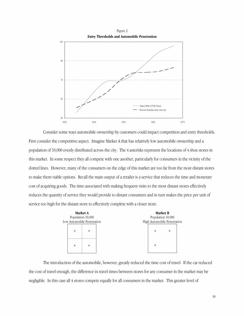
Heterogeneous Competition
One key departure of my specification of the profit function from that of Bresnahan and Reiss is to allow
for heterogeneous competition across markets. I do this to determine if any of the many socioeconomic changes
that occurred during the early 20th century altered the competitive landscape and in turn reduced or raised the
marginal effect of entry. The most likely candidate for such change is the introduction and spread of the
automobile.
Figure 2 shows the national time trend of automobile penetration along with the median sales per store,
which is strongly correlated with the entry threshold for a typical retail store. The rise in the size of retail stores
coincides with an increase in the use of the automobile.
18
Figure 2Entry Thresholds and Automobile Penetration
30
50
70
90
110
1935 1945 1955 1965 1975
Sales(1000 of 97$)/Store
Percent Families that own Car
Consider some ways automobile ownership by customers could impact competition and entry thresholds.
First consider the competitive aspect. Imagine Market A that has relatively low automobile ownership and a
population of 10,000 evenly distributed across the city. The 4 asterisks represent the locations of 4 shoe stores in
this market. In some respect they all compete with one another, particularly for consumers in the vicinity of the
dotted lines. However, many of the consumers on the edge of this market are too far from the most distant stores
to make them viable options. Recall the main output of a retailer is a service that reduces the time and monetary
cost of acquiring goods. The time associated with making frequent visits to the most distant stores effectively
reduces the quantity of service they would provide to distant consumers and in turn makes the price per unit of
service too high for the distant store to effectively complete with a closer store.
Market APopulation 10,000
Low Automobile Penetration
* *
* *
Market BPopulation 10,000
High Automobile Penetration
* *
*
The introduction of the automobile, however, greatly reduced the time cost of travel. If the car reduced
the cost of travel enough, the difference in travel times between stores for any consumer in the market may be
negligible. In this case all 4 stores compete equally for all consumers in the market. This greater level of
19
competition would tend to reduce price-cost margins and in turn variable profits. A market such as B might have a
similar size and market population but greater penetration of automobiles. The competition this fosters would
reduce variable profits to a greater extent with each subsequent entrant, possibly to the point that this market
could only support 3 stores.
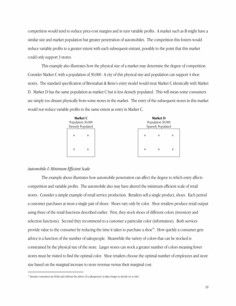
This example also illustrates how the physical size of a market may determine the degree of competition.
Consider Market C with a population of 30,000. A city of this physical size and population can support 4 shoe
stores. The standard specification of Bresnahan & Reiss’s entry model would treat Market C identically with Market
D. Market D has the same population as market C but is less densely populated. This will mean some consumers
are simply too distant physically from some stores in the market. The entry of the subsequent stores in this market
would not reduce variable profits to the same extent as entry in Market C.
Market CPopulation 30,000Densely Populated
* *
* *
Market DPopulation 30,000Sparsely Populated
* * *
* * *
Automobile & Minimum Efficient Scale
The example above illustrates how automobile penetration can affect the degree to which entry affects
competition and variable profits. The automobile also may have altered the minimum efficient scale of retail
stores. Consider a simple example of retail service production. Retailers sell a single product, shoes. Each period
a customer purchases at most a single pair of shoes. Shoes vary only by color. Shoe retailers produce retail output
using three of the retail functions described earlier. First, they stock shoes of different colors (inventory and
selection functions). Second they recommend to a customer a particular color (information). Both services
provide value to the consumer by reducing the time it takes to purchase a shoe14. How quickly a consumer gets
advice is a function of the number of salespeople. Meanwhile the variety of colors that can be stocked is
constrained by the physical size of the store. Larger stores can stock a greater number of colors meaning fewer
stores must be visited to find the optimal color. Shoe retailers choose the optimal number of employees and store
size based on the marginal increase to store revenue versus their marginal cost.
14 Assume consumers are fickle and without the advice of a salesperson, it takes longer to decide on a color.
20
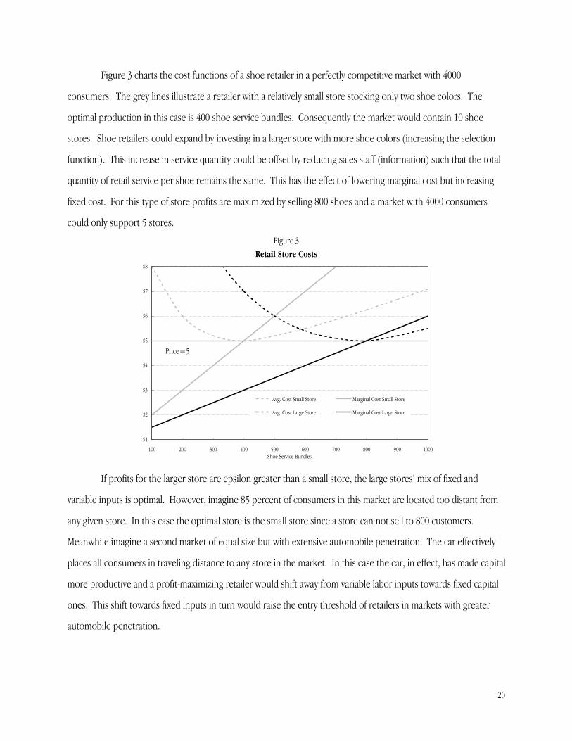
Figure 3 charts the cost functions of a shoe retailer in a perfectly competitive market with 4000
consumers. The grey lines illustrate a retailer with a relatively small store stocking only two shoe colors. The
optimal production in this case is 400 shoe service bundles. Consequently the market would contain 10 shoe
stores. Shoe retailers could expand by investing in a larger store with more shoe colors (increasing the selection
function). This increase in service quantity could be offset by reducing sales staff (information) such that the total
quantity of retail service per shoe remains the same. This has the effect of lowering marginal cost but increasing
fixed cost. For this type of store profits are maximized by selling 800 shoes and a market with 4000 consumers
could only support 5 stores.
Figure 3Retail Store Costs
$1
$2
$3
$4
$5
$6
$7
$8
100 200 300 400 500 600 700 800 900 1000Shoe Service Bundles
Avg. Cost Small Store Marginal Cost Small Store
Avg. Cost Large Store Marginal Cost Large Store
Price=5
If profits for the larger store are epsilon greater than a small store, the large stores’ mix of fixed and
variable inputs is optimal. However, imagine 85 percent of consumers in this market are located too distant from
any given store. In this case the optimal store is the small store since a store can not sell to 800 customers.
Meanwhile imagine a second market of equal size but with extensive automobile penetration. The car effectively
places all consumers in traveling distance to any store in the market. In this case the car, in effect, has made capital
more productive and a profit-maximizing retailer would shift away from variable labor inputs towards fixed capital
ones. This shift towards fixed inputs in turn would raise the entry threshold of retailers in markets with greater
automobile penetration.
21
IV. Estimation
Sample Selection & Data
The ideal data set for estimating entry thresholds would contain information on a single market where
demand has fluctuated enough to cause significant turnover. However, as Bresnahan and Reiss (1991b) note such
data is difficult to gather. Instead, following their lead, I use a cross section of geographically separated markets to
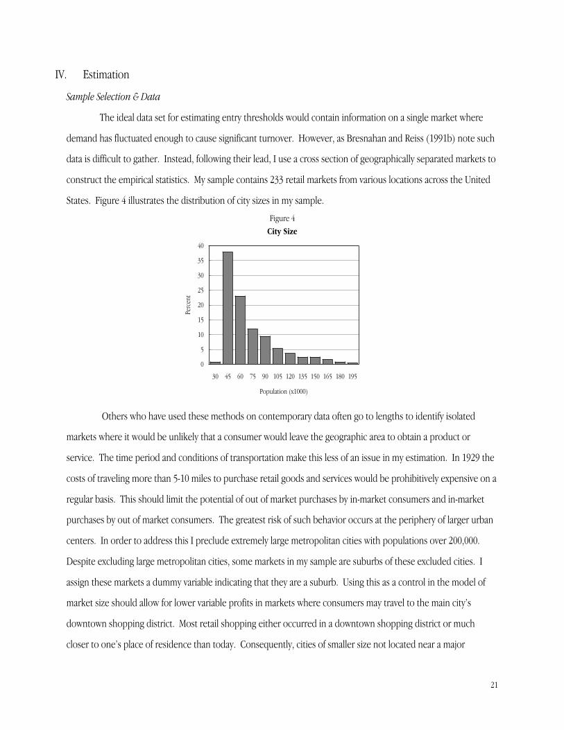
construct the empirical statistics. My sample contains 233 retail markets from various locations across the United
States. Figure 4 illustrates the distribution of city sizes in my sample.
Figure 4City Size
0
5
10
15
20
25
30
35
40
30 45 60 75 90 105 120 135 150 165 180 195
Population (x1000)
Perc
ent
Others who have used these methods on contemporary data often go to lengths to identify isolated
markets where it would be unlikely that a consumer would leave the geographic area to obtain a product or
service. The time period and conditions of transportation make this less of an issue in my estimation. In 1929 the
costs of traveling more than 5-10 miles to purchase retail goods and services would be prohibitively expensive on a
regular basis. This should limit the potential of out of market purchases by in-market consumers and in-market
purchases by out of market consumers. The greatest risk of such behavior occurs at the periphery of larger urban
centers. In order to address this I preclude extremely large metropolitan cities with populations over 200,000.
Despite excluding large metropolitan cities, some markets in my sample are suburbs of these excluded cities. I
assign these markets a dummy variable indicating that they are a suburb. Using this as a control in the model of
market size should allow for lower variable profits in markets where consumers may travel to the main city’s
downtown shopping district. Most retail shopping either occurred in a downtown shopping district or much
closer to one’s place of residence than today. Consequently, cities of smaller size not located near a major
22
metropolitan center were less susceptible to this demand leakage. On the other hand the population of the city
alone may not capture all demand for retail output from out of market consumers. Therefore I also use the
population of the county in which the city is located.
The primary source of data is the 1930 15th Census of the United States–Retail Distribution. It contains
information on over 100 different Census classifications of retail establishments. I divide my inquiry into store
types that are the primary source of a given product group15 and those that are not. For stores that are the former
there is more confidence that the store counts proxy for the total number of market competitors. Table 3 presents
a list of the retail segments examined as well as distribution information on the number of stores of each type in
markets.
Table 3Retail Store Segments
Store Counts per CityPrimary Source of Commodities
Sold Within MeanStandardDeviation Median Min Max
Book 1.9 2.0 1 0 12Jewelry 14.3 8.5 12 0 56
Opticians 3.0 3.2 2 0 17Additional Retail Stores
Department 4.2 2.7 4 0 13Variety 6.5 5.7 6 0 74Grocery 227.2 127.4 184 49 794
While the commodities sold by the last three types of stores in Table 3 were also sold in other types of
retail establishments, anecdotal evidence shows that these stores were viewed as unique types of establishments.
For example, Department stores and Variety stores sold similar types of commodities; however their store
structure, service model, and most importantly the quality of their goods were generally considered to be unique.
Predictors of N
Equation 10 in Section III specified the profit function for a retail store in a market k that has a total of N
stores,
€
ΠkN = α1 +Δ kδ −Χk
Vχ V − f Εkβ( ) ⋅ αnn=2
N
∑
Υkψ − g γ1 +Χk
vχ v( ) + γ nn=2
N
∑
+εk . While it is impossible
to observe Π, one can infer whether profits are positive or negative when there are different numbers of stores in
a market. In a Nash equilibrium if N stores are observed, ΠN must be greater than zero while ΠN+1 must be
negative. This fact allows the coefficients in Equation 10 to be estimated using maximum likelihood on a series of
15 Determined by national commodity sales data from the 1929 Retail Census.
23
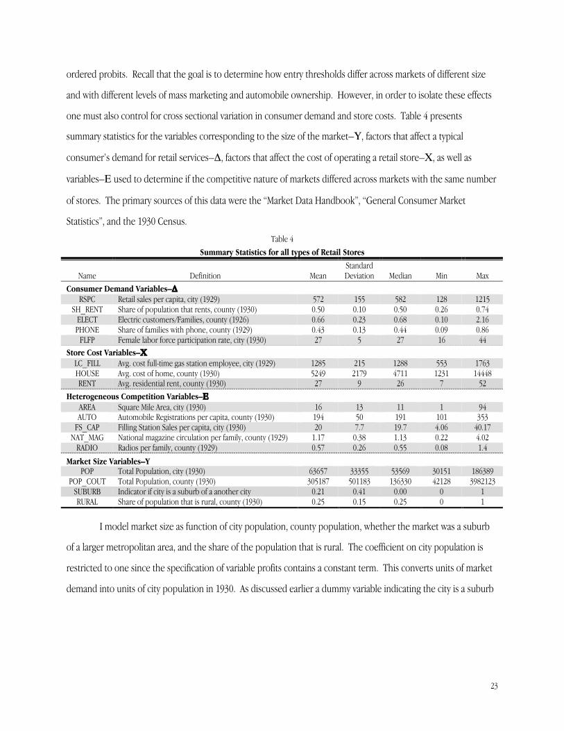
ordered probits. Recall that the goal is to determine how entry thresholds differ across markets of different size
and with different levels of mass marketing and automobile ownership. However, in order to isolate these effects
one must also control for cross sectional variation in consumer demand and store costs. Table 4 presents
summary statistics for the variables corresponding to the size of the market–Υ, factors that affect a typical
consumer’s demand for retail services–Δ, factors that affect the cost of operating a retail store–Χ, as well as
variables–Ε used to determine if the competitive nature of markets differed across markets with the same number
of stores. The primary sources of this data were the “Market Data Handbook”, “General Consumer Market
Statistics”, and the 1930 Census.
Table 4Summary Statistics for all types of Retail Stores
StandardName Definition Mean Deviation Median Min Max
Consumer Demand Variables–ΔRSPC Retail sales per capita, city (1929) 572 155 582 128 1215
SH_RENT Share of population that rents, county (1930) 0.50 0.10 0.50 0.26 0.74ELECT Electric customers/Families, county (1926) 0.66 0.23 0.68 0.10 2.16PHONE Share of families with phone, county (1929) 0.43 0.13 0.44 0.09 0.86
FLFP Female labor force participation rate, city (1930) 27 5 27 16 44Store Cost Variables–Χ
LC_FILL Avg. cost full-time gas station employee, city (1929) 1285 215 1288 553 1763HOUSE Avg. cost of home, county (1930) 5249 2179 4711 1231 14448RENT Avg. residential rent, county (1930) 27 9 26 7 52
Heterogeneous Competition Variables–ΕAREA Square Mile Area, city (1930) 16 13 11 1 94AUTO Automobile Registrations per capita, county (1930) 194 50 191 101 353
FS_CAP Filling Station Sales per capita, city (1930) 20 7.7 19.7 4.06 40.17NAT_MAG National magazine circulation per family, county (1929) 1.17 0.38 1.13 0.22 4.02
RADIO Radios per family, county (1929) 0.57 0.26 0.55 0.08 1.4
Market Size Variables–YPOP Total Population, city (1930) 63657 33355 53569 30151 186389
POP_COUT Total Population, county (1930) 305187 501183 136330 42128 3982123SUBURB Indicator if city is a suburb of a another city 0.21 0.41 0.00 0 1RURAL Share of population that is rural, county (1930) 0.25 0.15 0.25 0 1
I model market size as function of city population, county population, whether the market was a suburb
of a larger metropolitan area, and the share of the population that is rural. The coefficient on city population is
restricted to one since the specification of variable profits contains a constant term. This converts units of market
demand into units of city population in 1930. As discussed earlier a dummy variable indicating the city is a suburb

24
of a larger city controls for demand leakage. The population of the city’s county and the share of the county that
lives in a rural area control for any market demand not picked up by simple city population.16
Five variables constitute my matrix of consumer demand factors–Δ. Income should affect the demand for
retail services in two ways. People with greater income purchase more goods. Secondly, as I discuss in Section III
any factor that raises the cost of obtaining goods for consumption will raise the value or demand for retail services.
People with greater income often have a higher opportunity cost to their time, which would raise the cost of
obtaining goods and in turn raise the value of the services provided by retailers. Per capita total retail sales (RSPC)
is used to proxy for the income of the average consumer in each city. Other measures used to capture the wealth
of consumers in a market include the share that are renters, the use of electricity, and the share of families with a
phone in the home. The opportunity cost of search or shopping will also rise as more women are employed.
Consequently, the female labor force participation rate (FLFP) is included in Δ.
Retail operating cost variables consist of the labor cost of a full-time gas station worker17, the average cost
of a home, and the average residential rent. While information on the labor cost of employees in each segment is
available, this data is likely endogenous to entry and input decisions. Consequently the cost of a gas station worker
is used to proxy for the cost of a retail employee in each segment. Gas stations were chosen due to their
consistent presence and general uniformity across markets. Labor costs are included in the variable profits
component of the profit function to control for cities with higher variable operating costs. Higher labor costs
would have the effect of lowering variable profits and raising entry thresholds. A market’s average cost of a home
and residential rent are included in the fixed cost of a store’s profit function. These figures proxy for a store’s
actual fixed cost of rent or their building. Finally, in order to determine if retailers in markets with greater
automobile penetration were induced to shift toward fixed cost inputs, the fixed cost component of the profit
function also contains a measure of car ownership.
The vector Ε allows competition to differ across markets with the same number of stores. Four variables
constitute Ε: a measure of automobile penetration18, the size of the city in square miles, the circulation of 5
national magazines per family, and the number of radios per family. I previously discussed the logic behind
including measures of automobile penetration and the physical size of the city. National magazine circulation is
16 Many other similar studies use some measure of population growth to control for future population size. This was attempted, however, the coefficient of populationgrowth was always statistically insignificant in explaining store count variations across markets.17 Employee counts, payroll, and other expense information reported in the Retail Census are used to construct the gas station figure.18 Filling station sales per capita or automobile registrations per capita are used depending on which maximizes the Likelihood function for a given segment.
25
included to determine if national branded mass marketed goods had any effect on retailers early in the century.
Martha Olney shows in her book “Buy Now Pay Later” that a substantial increase in national advertising happened
during the 1920s. Between 4 to 6 times more money was spent in each year of the decade than had been spent in
1915.19 Advertising by manufacturers provided valuable information to consumers about the products they would
find at local retailers. This may in turn have reduced the value added the retailer could produce through the
information function. If this occurred one might expect variable profits to fall more with the entry of subsequent
stores. A measure of radio penetration is included for similar reasons. The radio, however, also had local
programming and advertising. This local advertising might have created greater competition as information could
be delivered to even distant consumers. Conversely, the radio may have allowed greater product differentiation
within a market.
By using the number of stores per market in an ordered probit framework, the coefficients in Equation 10
can be estimated. These coefficients can then be used to construct entry thresholds or the population size a
typical city requires to support N stores. If one observes that per store entry thresholds are significantly larger in
markets with fewer stores it suggests the stores in these markets are exercising market power by pricing above
average cost. However the fact that these per store thresholds fall with the number of stores in a market suggests
that entry exerts competitive pressure and this power to mark-up diminishes. If entry thresholds reach a point
such that they rise proportionately with the number of stores one might infer that market is competitive. This is
because there are enough competitors in the market to have driven price to average cost and economic profits are
zero20. Further inferences can be drawn about the competitive nature of retailers by examining how entry
thresholds differ with changes in the market characteristics in vector Ε. If a variable like automobile penetration
increases competition, one will see larger entry thresholds in markets with 2 or more stores and higher rates of car
ownership. If this hypothesis is confirmed it might provide one explanation of why retail store size rose
significantly during the first half of the 20th century.
Estimation Results
The coefficient estimates from the ordered probit of Equation 10 are reported in Table A.1 of the
appendix. The coefficients themselves are difficult to interpret due to the non-linearity of the probit model.
However, because the markets used in this study are less homogeneous than those used in many other entry
19 P. 138 Olney (1991)20 Note, an alternative explanation could be that after 4 or 5 stores enter the market the stores agree on a collusive price.
26
papers, it is important how well the consumer demand and store costs variables control for possible variations in
variable profits and fixed costs unrelated to entry.
Each segment has a number of controls that significantly explain variation in consumer demand and store
costs. For nearly every segment either average rents or house costs statistically significantly account for fixed cost
variation. In other words, a store in a market with higher rents appears to have greater fixed costs. The coefficient
on retail sales per capita is positive and statistically significant for every segment. Recall retail sales per capita proxy
for the income of consumers in the market, which when higher should increase demand for retail services and
raise per capita variable profits. The share of the renter population seems to indicate that more renters are
associated with lower per capita variable profits. Using the number of electrical customers and phones as a control
for wealth does not appear to have any consistent relationship with entry thresholds, but for many sectors their
coefficients are statistically significant. Using the labor cost of gas stations has mixed results in controlling for
differences in variable costs. As one would expect for all but the Department store segment, high gas station labor
costs are associated with higher labor costs in the respective retail segment–though only 2 coefficients are
statistically significant. Finally, greater female labor force participation may have been associated with higher
variable profits; however, only the coefficients for Book and Optical Stores are statistically significant.
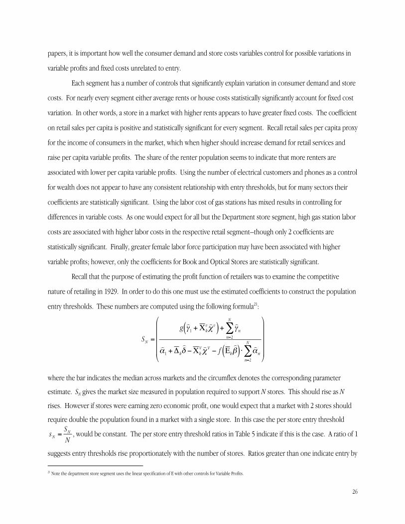
Recall that the purpose of estimating the profit function of retailers was to examine the competitive
nature of retailing in 1929. In order to do this one must use the estimated coefficients to construct the population
entry thresholds. These numbers are computed using the following formula21:
€
S N =
g ) γ 1 +Χ k
v ) χ v( ) +
) γ n
n=2
N
∑
) α 1 +Δ k
) δ −Χ k
V ) χ V − f Ε k
) β ( ) ⋅ )
α nn=2
N
∑
where the bar indicates the median across markets and the circumflex denotes the corresponding parameter
estimate. SN gives the market size measured in population required to support N stores. This should rise as N
rises. However if stores were earning zero economic profit, one would expect that a market with 2 stores should
require double the population found in a market with a single store. In this case the per store entry threshold
€
s N =S N
N, would be constant. The per store entry threshold ratios in Table 5 indicate if this is the case. A ratio of 1
suggests entry thresholds rise proportionately with the number of stores. Ratios greater than one indicate entry by
21 Note the department store segment uses the linear specification of E with other controls for Variable Profits.
27
subsequent stores requires a greater per store population. This could occur in settings where a monopolist or
duopolist exercises market power. Note, economic theory provides some hint at how these ratios should look. If
retail stores compete in a homogeneous product, Bertrand competitive setting, one would expect the first ratio
s2/s1 to be large but all remaining ratios equal to 1. This is, of course, because the entry of one additional store
drives the market to price at marginal cost. Cournot competition with homogeneous products would predict a
gradual decline toward 1 as N approaches infinity. Note, if stores are able to differentiate their products these
ratios would fall more gradually.Table 5
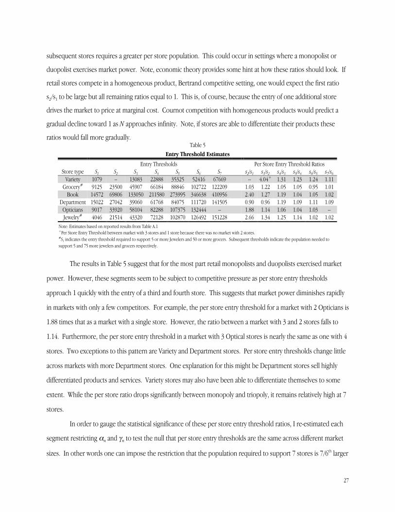
Entry Threshold Estimates
� Entry Thresholds � Per Store Entry Threshold RatiosStore type S1 S2 S3 S4 S5 S6 S7 � s2/s1 s3/s2 s4/s3 s5/s4 s6/s5 s7/s6
Variety 1079 -- 13083 22888 35325 52416 67669 � -- 4.04+ 1.31 1.23 1.24 1.11Grocery# 9125 23500 45907 66184 88846 102722 122209 1.03 1.22 1.05 1.05 0.95 1.01
Book 14572 69806 133050 211580 273995 346638 410956 � 2.40 1.27 1.19 1.04 1.05 1.02Department 15022 27042 39060 61768 84075 111720 141505 0.90 0.96 1.19 1.09 1.11 1.09
Opticians 9017 33920 58104 82288 107375 132444 -- � 1.88 1.14 1.06 1.04 1.03 --Jewelry# 4046 21514 43320 72128 102870 126492 151228 � 2.66 1.34 1.25 1.14 1.02 1.02
Note: Estimates based on reported results from Table A.1+Per Store Entry Threshold between market with 3 stores and 1 store because there was no market with 2 stores.#S1 indicates the entry threshold required to support 5 or more Jewelers and 50 or more grocers. Subsequent thresholds indicate the population needed tosupport 5 and 75 more jewelers and grocers respectively.
The results in Table 5 suggest that for the most part retail monopolists and duopolists exercised market
power. However, these segments seem to be subject to competitive pressure as per store entry thresholds
approach 1 quickly with the entry of a third and fourth store. This suggests that market power diminishes rapidly
in markets with only a few competitors. For example, the per store entry threshold for a market with 2 Opticians is
1.88 times that as a market with a single store. However, the ratio between a market with 3 and 2 stores falls to
1.14. Furthermore, the per store entry threshold in a market with 3 Optical stores is nearly the same as one with 4
stores. Two exceptions to this pattern are Variety and Department stores. Per store entry thresholds change little
across markets with more Department stores. One explanation for this might be Department stores sell highly
differentiated products and services. Variety stores may also have been able to differentiate themselves to some
extent. While the per store ratio drops significantly between monopoly and triopoly, it remains relatively high at 7
stores.
In order to gauge the statistical significance of these per store entry threshold ratios, I re-estimated each
segment restricting αn and γn to test the null that per store entry thresholds are the same across different market
sizes. In other words one can impose the restriction that the population required to support 7 stores is 7/6th larger
28
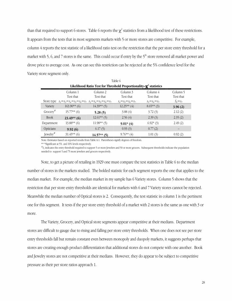
than that required to support 6 stores. Table 6 reports the χ2 statistics from a likelihood test of these restrictions.
It appears from the tests that in most segments markets with 5 or more stores are competitive. For example,
column 4 reports the test statistic of a likelihood ratio test on the restriction that the per store entry threshold for a
market with 5, 6, and 7 stores is the same. This could occur if entry by the 5th store removed all market power and
drove price to average cost. As one can see this restriction can be rejected at the 5% confidence level for the
Variety store segment only.
Table 6Likelihood Ratio Test for Threshold Proportionality–χ2 statistics
Column 1 Column 2 Column 3 Column 4 Column 5� Test that Test that Test that Test that Test that
Store type s2=s3=s4=s5=s6=s7 s3=s4=s5=s6=s7 s4=s5=s6=s7 s5=s6=s7 S6=s7
Variety 163.90** (6) 14.39** (5) 12.25** (4) 8.65** (3) 3.96 (2)Grocery# 15.77** (6) 5.28 (5) 3.88 (4) 3.72 (3) 2.12 (2)
Book 23.49** (6) 12.61** (5) 2.56 (4) 2.39 (3) 2.35 (2)Department 13.88** (6) 11.98** (5) 9.01* (4) 6.92* (3) 2.49 (2)
Opticians 9.92 (6) 6.17 (5) 0.93 (3) 0.77 (2) --
Jewelry# 31.45** (6) 14.57** (5) 9.76** (4) 1.01 (3) 0.92 (2)Note: Estimates based on reported results from Table A.1. Parentheses signify degrees of freedom.** *Significant at 5% and 10% levels respectively.#S1 indicates the entry threshold required to support 5 or more Jewelers and 50 or more grocers. Subsequent thresholds indicate the populationneeded to support 5 and 75 more jewelers and grocers respectively.
Note, to get a picture of retailing in 1929 one must compare the test statistics in Table 6 to the median
number of stores in the markets studied. The bolded statistic for each segment reports the one that applies to the
median market. For example, the median market in my sample has 6 Variety stores. Column 5 shows that the
restriction that per store entry thresholds are identical for markets with 6 and 7 Variety stores cannot be rejected.
Meanwhile the median number of Optical stores is 2. Consequently, the test statistic in column 1 is the pertinent
one for this segment. It tests if the per store entry threshold of a market with 2 stores is the same as one with 3 or
more.
The Variety, Grocery, and Optical store segments appear competitive at their medians. Department
stores are difficult to gauge due to rising and falling per store entry thresholds. When one does not see per store
entry thresholds fall but remain constant even between monopoly and duopoly markets, it suggests perhaps that
stores are creating enough product differentiation that additional stores do not compete with one another. Book
and Jewelry stores are not competitive at their medians. However, they do appear to be subject to competitive
pressure as their per store ratios approach 1.
29
Another goal of this paper is to isolate any effects the spread of the automobile and changes in mass
marketing had on competition and entry thresholds. One clear result from the data is that entry thresholds differ
based on these factors. Contrary to what one might expect, entry by stores in larger physical markets had a greater
effect on variable profits than on more densely populated markets. For the most part markets with more national
magazine subscription rates appear to see larger drops in variable profits in markets with more stores. However,
this effect is never statistically significant. Perhaps the most consistent and statistically significant result from
estimating these series of ordered probits is the effect of radio ownership on competitive conduct. In every
segment except Department stores greater radio ownership is associated with a smaller drop in variable profits for
markets with more than one store. This suggests less competition among stores in markets with high radio
ownership. One might suspect radio ownership acts as another proxy for wealth; however, in all these segments
likelihood ratio tests rejected that radio should enter the variable profits section. These results suggest that the
radio and perhaps the local advertising on it allowed retailers to better differentiate their products.
Analyzing the relationship between car ownership and entry thresholds is complicated by the fact that in
most specifications auto penetration appears in both the fixed cost and variable profit components of the profit
function. However, it is clear that the car affected entry thresholds. In every case but Book stores, markets with
more car ownership are associated with higher entry thresholds either through greater fixed costs, by increasing
the effect of entry on variable profits, or both.
Table 7Significance and Magnitude of Heterogeneous Entry Effects
Column 1 Column 2 Column 3 Column 4
Store type
Difference in EntryThreshold at Medianbetween cities 1 STDbelow and above the
median autopenetration
χ2–test that Auto hasno affect on Entry
Thresholds
Difference in EntryThreshold at Medianbetween cities 1 STDbelow and above the
median radiopenetration
T-test that Radio hasno affect on Entry
ThresholdsVariety 8.17% 4.81* (2) -24.48% 1.74*Grocery 8.86% 7.84** (2) -5.04% 1.22
Book -0.92% 2.36 (2) -48.01% 3.23**Department+ 9.79% 0.39 (1) 65.23% 4.42**
Opticians 3.27% 0.25 (2) -4.42% 1.53Jewelry 9.96% 4.84* (2) -20.12% 2.27**
Note: Estimates based on full model, ** * indicate significance at 5 & 10 percent respectively+Heterogeneous Entry Variables contained in simple Variable Profit section
Table 7 reports the magnitude and statistical significance of automobile and radio ownership on entry
thresholds. The first column reports how much larger a city with above average car ownership would need to be
30
verses one with below average ownership to support each segment’s median number of stores. In every segment
except Book, automobile penetration raises entry thresholds. Column 2 of Table 7 reports χ2–tests on the null
that automobile penetration had no effect on either competition or fixed costs. Car ownership has a statistically
significant effect in the Variety, Grocery, and Jewelry segments. In each case the rise in auto mobile penetration is
associated with an over 8% increase in the population entry threshold required to support the median number of
stores in my sample.
Columns three and four report similar statistics for radio ownership. Since this control only enters one
part of the profit function, t-tests are conducted to test for a statistically significant effect. Entry Thresholds for
Variety, Book, Department, and Jewelry stores are significantly affected by rates of radio ownership. In all
segments except Department stores higher rates of ownership reduce the effect of entry and entry thresholds.
Generally the magnitude of this effect is large when compared with automobile penetration. Meanwhile radio
ownership seems to have an opposite and large effect on Department stores–reducing variable profits and raising
entry thresholds. Given radio use and advertising only expanded in the years after 1929, this result would seem to
predict decreasing entry thresholds or store size. One possible explanation is a change in the type of radio
advertising. White (1971) notes in his book, “History of Broadcasting: Radio to Television”, that early radio
advertisements were viewed as intrusive. Sometimes actual sales pitches were banned. Consequently, radio ads in
the 20’s were prominently in the form of program sponsorships where the name of a product, store, or
manufacturer was featured as the sponsor of an hour of music or comedy show. One would expect these type of
ads to create store differentiation, which would reduce the effect of competition and entry just as the estimations
above suggest. However, as radio advertising moved towards more product and sale oriented information, the
effect of radio penetration could switch to increasing competition and raising entry thresholds22. If this was the
case perhaps the most significant part of the radio results above is the magnitude of the effect.
V. Conclusions
The retail industry has undergone substantial change over the last 100 years. The roots of this change
began in the first three decades of the 20th century. The size or entry thresholds of retailers were beginning to
change as small stores were replaced with larger ones serving more people per store. This change renewed debate
22 This is similar to Bagwell & Ramey(1994), where advertising is shown to raise concentration.
31
over the efficiency and competitiveness of retailers, though at the time economists had little data and few methods
for exploring these issues.
This paper employs modern empirical techniques to provide insight on these two issues by comparing
estimated entry thresholds across markets. It also identifies factors that changed the competitive nature of a retail
market. I find that per store entry threshold ratios fall sharply after the entry of second and third stores in a
market. This suggests retailers were subjected to greater competitive pressures as the number of competitors
increased. Generally markets with five or more stores appear to be competitive as measured by per store entry
threshold ratios. In other words stores no longer exercise significant market power. However, the estimates
suggests that retailers in smaller markets with fewer stores exercised some market power and for certain segments
this was the more typical case.
The estimations also find that the effect of entry varied with certain characteristics of the market. Namely
radio ownership seems to have mitigated the effects of entry or lowered entry thresholds for markets with more
than 1 store. A likely cause of this is exposure to greater local radio advertising. While advertising could have
increased the level of competition as price and product comparisons became less costly, the result suggests that
local advertisement allowed greater product differentiation by retailers. Another factor explored was the effect of
the automobile. After developing a model of how and why car ownership could alter store size or entry
thresholds, I find some evidence that markets with more automobiles had higher entry thresholds. This suggests
that the further adoption of automobiles over the rest of the century may explain in part the rise in store size,
either by shifting production costs toward more fixed inputs or by expanding the scope of competition between
stores in a market.
These results are important because they show retailers were subject to competitive pressure as the
number of stores in a market increased. The degree of this competition did, however, differ across markets with
more or less automobile and radio ownership. While the radio is associated with lower entry thresholds or smaller
stores, radio advertising at the time was focused on product differentiation and name recognition. As broadcast
advertising moved towards a more price and product focus, the effect of radio may have switched. Given how
large the estimated effect of radio ownership was on entry threshold this might explain a significant portion of the
rise in store size during the first half of the 20th century. The estimated effect of the automobile was smaller.
However, there is clear evidence that the car raised entry thresholds. Given car ownership rates only increased
further over the next 30 years, this too might explain a good portion of rising store size.
32
VI. References
Appel, David (1972), “The Supermarket: Early Development of an Institutional Innovation,” Journal of Retailing,48, 39-53.
Arndt, J. and L. Olsen (1975), “A research Note on Economies of Scale in Retailing,” Swedish Journal of Economics,77, 205-228.
Bagwell, Kyle and Garey Ramey (1994), “Coordination Economies, Advertising, and Search Behavior in RetailMarkets,” American Economic Review, 84(3), 498-517.
Bagwell, Kyle, Garey Ramey and Daniel F. Spulber (1997), “Dynamic retail price and investment competition,”RAND Journal of Economics, 28(2), 207-227.
Bain, J., (1956), Barriers to New Competition, Harvard University Press, Cambridge.
Barger, Harold (1955), Distribution’s Place in the American Economy since 1869, Princeton, NJ: PrincetonUniversity Press.
Bellamy, R. (1946), “The Changing Pattern of Retail Distribution,” Bulletin of the Oxford University Institute ofStatistics, 8(August), 237-60.
–––––––– (1946b), “Private and Social Cost in Retail Distribution,” Bulletin of the Oxford University Institute ofStatistics, 8(November), 345-51.
–––––––– (1946c), “Size and Success in Retail Distribution,” Bulletin of the Oxford University Institute ofStatistics, 8(October), 324-39.
Benson, Johnson and Laura Ugolini (2003), A Nation of Shopkeepers: Five Centuries of British Retailing, London:I.B. Tauris & Co Ltd.
Berry, Steven T., (1992), “Estimation of a Model of Entry in the Airline Industry,” Econometrica, 60(4), 889-917.
Berry, Steven T. and Joel Waldfogel (1999), “Free Entry and Social Inefficiency in Radio Broadcasting,” RandJournal of Economics, 30(3), 397-420.
Betancourt, Roger and David Gautschi (1990), “Demand Complementarities, Household Production, and RetailAssortments,” Marketing Science, 9, 2(Spring), 146-161.
–––––––– and ––––––– (1993), “The Outputs of Retail activities: Concepts, Measurement and Evidence fromthe U.S. Census Data,” Review of Economics and Statistics, 75, 2(May), 294-301.
33
Bresnahan, Timothy F. (1989), “Empirical Studies of industries with market power.” Handbook of IndustrialOrganization, vol. 2, North-Holland, Amsterdam.
Bresnahan, Timothy F. and Peter C. Reiss (1991a), “Empirical Models of Discrete Games,” Journal ofEconometrics, 48(1), 57-81.
Bresnahan, Timothy F. and Peter C. Reiss (1991b), “Entry and Competition in Concentrated Markets,” Journal ofPolitical Economy, 99(5), 977-1009.
Bresnahan, Timothy F. and Peter C. Reiss (1990), “Entry in Monopoly Markets,” Review of Economic Studies, 57,531-553.
Bresnahan, Timothy F. and Peter C. Reiss (1987), “Do Entry Conditions Vary Across Markets?” Brookings Paper onEconomic Activity, 3, 833-871.
Bucklin, Louis P. (1972), Competition and Evolution in the Distributive Trades, Englewood Cliffs, NJ: Prentice-HallInc.
Cohen, Leonard (1951), “Costs of Distribution in Department Stores,” Manchester School of Economic and SocialStudies, 20(May), 139-73.
Davis, Peter J. (1998), “Spatial Competition in Retail Markets: Movie Theatres,” working paper.
Douglas, E. (1962), “Size of Firm and the Structure of Costs in Retailing,” Journal of Business, 25(April), 158-190.
Downes, T., and S. Greenstein, (1996), “Understanding the supply decisions of non-profits: modeling the locationof private schools”, Rand Journal of Economics, 27, 365-390.
Hall, Margaret and John Knapp (1955), “Gross Margins and Efficiency Measurement in Retail Trade,” OxfordEconomic Papers, 7(3), 312-326.
Hall, Margaret, John Knapp and C. Winsten (1961), Distribution in Great Britain and North America, London:Oxford University Press.
Hausman, J., Leonard, G., and D. Zona, (1994), “Competitive analysis with differentiated products,” Annalesd’Economie et de Statistique, 0, 159-180.
Hower, R.M. (1943), The History of Macy’s of New York 1858-1919: chapters in the evolution of the departmentstore, Harvard University Press, Cambridge, Mass.
ICPSR (Inter-university Consortium for Political and Social Research), “County and City Data Book [United States]Consolidated File: City Data 1944-1977,” #7735, conducted by the Bureau of the Census, Washington:The Bureau, 1978.
34
Ingene, Charles A. (1984), “Scale Economies in American Retailing: a Cross-Industry Comparison,” Journal ofMacromarketing (Fall), 49-63.
Mann, Lawrence B. (1923), “The Importance of Retail Trade in the United States,” The American EconomicReview, 13(4), 609-617.
Manuszak, M.D., (2002), “Endogenous market structure and competition in the 19th century American brewingindustry,” International Journal of Industrial Organization, 20, 673-692.
Mazzeo, Michael J., (2002), “"Product Choice and Oligopoly Market Structure," Rand Journal of Economics,(Summer).
Messinger, Paul R. and Chakravarthi Narasimhan (1997), “A Model of Retail Formats Based on Consumers’Economizing on Shopping Time,” Marketing Science, 16, 1, 1-23.
McClelland, W. (1972), “Economics of the Supermarket,” Economic Journal, March, 154-70.
––––––––– (1966), Costs and Competition in Retailing, London: Macmillan.
Olney, Martha L., (1991), Buy Now Pay Later, Chapel Hill, N.C.: The University of North Carolina Press.
Reiss, Peter C. (1996), “Empirical Models of Discrete Strategic Choices,” American Economic Review, 86(2), 421-426.
Reiss, Peter C. and Pablo T. Spiller (1989), “Competition and entry in Small Airline Markets,” Journal of Law andEconomics, 32, S179-S202.
Savitt, R. (1975), “Economies of Scale in Canadian Supermarkets,” Canadian Association of AdministrativeScience, Conference Proceedings, Edmonton: University of Alberta.
Spulber, Daniel, (1999), Market Microstructure, Cambridge: Cambridge University Press.
Stavins, J., (1995), “Model entry and exit in a differentiated-products industry: the personal computer market,”Review of Economics and Statistics, 77, 571-584.
Tilly, R. and R. Hicks (1970), “Economies of Scale in Supermarkets,” Journal of Industrial Economics,19(November), 1-5.
Tucker (1975), Economies of Scale in Retailing: an empirical study of plant size and cost structure, London:Saxon House.
Offer, G. (1973), “Returns to Scale in Retail Trade,” Review of Income and Wealth, 19(December), 363-384.
35
U.S. Bureau of the Census, Fifteenth Census of the United States–Retail Distribution, Washington DC: Govt.Printing Office, 1933.
U.S. Bureau of the Census, 1997 Economic Census, Retail Trade, Washington DC: Govt. Printing Office, 2001.
U.S. Department of the Commerce, General Consumer Market Statistics, Washington DC: Govt. Printing Office,1932.
Whiteley, A.S. (1936), “Retail Trade in the United States and Canada,” The Journal of Political Economy, 44(1), 54-69.
White, Llewellyn. (1971), History of Broadcasting: Radio to Television–the American Radio, Arnos Press & The NewYork Times.
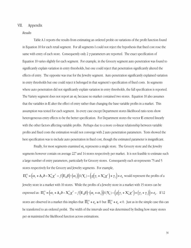
36
VII. Appendix
Results
Table A.1 reports the results from estimating an ordered probit on variations of the profit function found
in Equation 10 for each retail segment. For all segments I could not reject the hypothesis that fixed cost rose the
same with entry of each store. Consequently only 2 γ parameters are reported. The exact specification of
Equation 10 varies slightly for each segment. For example, in the Grocery segment auto penetration was found to
significantly explain variation in entry thresholds, but one could reject that penetration significantly altered the
effects of entry. The opposite was true for the Jewelry segment. Auto penetration significantly explained variation
in entry thresholds but one could reject it belonged in that segment’s specification of fixed costs. In segments
where auto penetration did not significantly explain variation in entry thresholds, the full specification is reported.
The Variety segment does not report an α2 because no market contained two stores. Equation 10 also assumes
that the variables in Ε alter the effect of entry rather than changing the base variable profits in a market. This
assumption was tested for each segment. In every case except Department stores likelihood ratio tests show
heterogeneous entry effects to be the better specification. For Department stores the vector Ε entered linearly
with the other factors affecting variable profits. Perhaps due to a more co-linear relationship between variable
profits and fixed costs the estimation would not converge with 2 auto penetration parameters. Tests showed the
best specification was to include auto penetration in fixed cost, though the estimated parameter is insignificant.
Finally, for most segments examined αn represents a single store. The Grocery store and the Jewelry
segments however contain on average 227 and 14 stores respectively per market. It is not feasible to estimate such
a large number of entry parameters, particularly for Grocery stores. Consequently each α represents 75 and 5
stores respectively for the Grocery and Jewelry segments. For example,
€
Πk10 = α1 +Δ kδ −Χk
Vχ V − f Εkβ( ) ⋅ α2( )( )S(Υk )− g γ1 +Χkvχ v( ) + γ2( ) +εk would represent the profits of a
Jewelry store in a market with 10 stores. While the profits of a Jewelry store in a market with 15 stores can be
expressed as:
€
Πk15 = α1 +Δ kδ −Χk
Vχ V − f Εkβ( ) ⋅ α2 +α 3( )( )S(Υk )− g γ1 +Χkvχ v( ) + γ2 + γ2( )( ) +εk . If 12
stores are observed in a market this implies that
€
Π k10 +εk ≥ 0 but
€
Π k15 +εk < 0 . Just as in the simple case this can
be transferred to an ordered probit. The width of the intervals used was determined by finding how many stores
per α maximized the likelihood function across estimations.
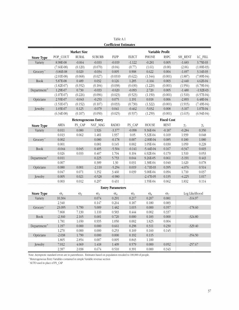
37
Table A.1Coefficient Estimates
� Market Size Variable Profit
Store Type POP_COUT RURAL SUBURB FLFP ELECT PHONE RSPC SH_RENT LC_FILLVariety 8.98E-08 -0.064 -0.033 -0.019 -1.122 -0.281 0.005 -1.683 3.75E-03
(7.66E-08) (0.120) (0.070) (0.04) (0.77) (1.61) (0.00) (2.06) (1.00E-03)Grocery~ -3.86E-08 0.020 -0.034 0.005 0.908 0.622 0.004 -1.697 3.14E-03
(2.01E-08) (0.068) (0.027) (0.0310 (0.622) (1.344) (0.001) (1.887) (7.89E-04)Book 5.87E-08 0.489 0.032 0.126 1.285 -1.166 0.003 -2.440 4.62E-04
(1.82E-07) (0.352) (0.184) (0.038) (0.630) (1.220) (0.001) (1.956) (6.79E-04)Department+ 1.29E-07 0.730 -0.033 -0.020 -0.093 2.720 0.005 -1.480 -1.92E-03
(1.07E-07) (0.226) (0.096) (0.023) (0.523) (1.150) (0.001) (1.510) (6.57E-04)Opticians 2.55E-07 -0.043 -0.253 0.075 1.191 0.018 0.006 -2.893 6.48E-04
(1.51E-07) (0.152) (0.107) (0.033) (0.730) (1.322) (0.001) (1.915) (7.49E-04)Jewelry 1.65E-07 0.125 -0.079 0.041 -0.462 -5.032 0.008 -3.107 1.07E-04
(6.34E-08) (0.107) (0.050) (0.025) (0.537) (1.259) (0.001) (1.615) (6.94E-04)
Heterogeneous Entry Fixed Cost
Store Type AREA FS_CAP NAT_MAG RADIO FS_CAP HOUSE RENT γ1 γn
Variety 0.011 0.080 1.926 -3.377 -0.098 9.36E-04 -0.187 -0.284 0.3500.013 0.062 1.481 1.937 0.05 5.32E-04 0.169 1.939 0.048
Grocery~ 0.002 0.080 -0.178 0.007 -2.00E-04 0.085 0.180 1.0800.001 0.081 0.145 0.002 1.05E-04 0.030 1.059 0.228
Book -0.044 0.045 0.405 -5.504 -0.141 -5.44E-04 0.167 -0.347 0.6030.026 0.033 0.407 1.704 0.104 6.92E-04 0.170 1.510 0.053
Department+ 0.011 0.225 5.753 0.044 9.26E-05 0.061 -3.191 0.4430.007 0.389 1.30 0.031 1.38E-04 0.040 1.620 0.078
Opticians 0.080 0.001 -2.110 -5.294 0.019 -1.71E-03 0.395 -4.076 0.5140.047 0.071 1.352 3.460 0.039 5.00E-04 0.094 1.710 0.037
Jewelry 0.005 0.021 -0.528 -0.980 � -2.47E-05 0.135 -4.225 1.0170.003 0.012 0.297 0.431 1.55E-04 0.062 1.832 0.114
Entry Parameters
Store Type α1 α2 α3 α4 α5 α6 α7 Log LikelihoodVariety 10.304 0.074 0.291 0.217 0.207 0.081 -314.97
2.340 0.147 0.264 0.187 0.180 0.083 �Grocery~ 23.095 5.790 5.009 1.482 1.015 0.000 0.357 -178.60
7.868 7.130 1.110 0.583 0.444 0.002 0.337 �Book -2.360 2.165 0.681 0.720 0.000 0.183 0.000 -324.80
1.781 1.650 0.935 1.050 0.002 1.825 0.004 �Department+ 1.197 0.000 0.000 0.661 0.298 0.311 0.230 -329.40
1.270 0.000 0.000 0.253 0.169 0.160 0.145 �Opticians -2.038 1.790 0.000 0.000 0.192 0.115 -354.50
1.865 2.854 0.007 0.005 0.843 1.100 �Jewelry 7.012 4.069 1.418 1.409 0.579 0.000 0.052 -257.67
2.397 2.038 0.674 0.510 0.391 0.000 0.343 �Note: Asymptotic standard errors are in parentheses. Estimates based on population rescaled to 100,000 of people.+Heterogeneous Entry Variables contained in simple Variable revenue section~AUTO used in place of FS_CAP
38
Table A.1 separates the parameter estimates into those affecting the Market Size, Variable Profit,
Heterogeneous Entry, Fixed Costs, and the actual dummy Entry Parameters. For the most part the estimates on
Market Size are what one would expect. More populous counties tend to raise the number of consumers in a
given market. The Suburb parameter is negative for all but Bookstores. This suggests a close large urban center
tends to reduce the number of consumers in a market of a given population size. Being in a rural area does not
seem to have any consistent relationship to market size and is generally insignificant. One exception is the
Department store segment. This suggests that Department stores exist in rural areas may attract customers from
more distant locations.
The markets used in this study are less homogenous than those used in many other entry papers.
Consequently the controls for variable profits across markets are important. Each segment has a number of
controls that significantly explain variation in entry thresholds. Retail sales per capita is highly statistically
significant for every segment. The share of the population that rents seems to indicate renters are associated with
lower variable profits, though in most cases statistically insignificant. Using the number of electrical customers and
phones as a control for wealth does not appear to have any consistent relationship with entry thresholds, but for
certain sectors is statistically significant. Using the labor cost of gas stations has mixed results controlling for
differences in variable costs. As one would expect for all but the Department store segment, high gas station labor
costs are associated with higher labor costs in the respective retail segment- though only two are statistically
significant. Finally, there is mixed success attempting to discern the effect greater female labor force participation
may have had on the industry. Four of the six segments saw higher variable profits in markets where more women
worked. Yet, only for Book and Optical stores was the effect significant.
Table A.2Test for Linear Rising Fixed Cost
� Test thatStore type γ2=γ3=γ4=γ5=γ6=γ7
Variety 8.76 (4)Grocery 6.67 (5)
Book 6.54 (5)Department 3.32 (5)
Opticians 4.21 (4)Jewelry 7.73 (5)
Note: Estimates based on reported results fromTable A.1. Parentheses signify degrees of freedom.
39
Turning to the controls on fixed cost across markets, one can see that for nearly every segment either
average rents or house costs significantly account for cost variation. Fixed costs also appear to rise consistently
with entry of subsequent stores. The relationship between fixed cost and automobile penetration is less consistent
or precise. Analyzing this relationship and entry thresholds is complicated by the fact that in most specifications
auto penetration appears in both the fixed cost and the heterogeneous entry effect components of the profit
function. What is clear is that the data could not well distinguish through what mechanism auto penetration may
have changed entry thresholds. One exception is the Grocery store segment where auto penetration could be
rejected as belonging in the heterogeneous entry component, but was statistically significant in explaining
differences in fixed costs across markets. Meanwhile the opposite was true for Jewelry stores.
One clear result from the data is that entry affects stores differently across markets. As discussed above
only for Department stores did the area, car penetration, and advertising variables enter linearly with the other
variable profit controls. For the other segments a positive sign on these controls can be interpreted as increasing
the effect of entry. In other words in every case automobile penetration raised how much entry of subsequent
stores lowered variable profits. Contrary to what one might expect entry by stores in larger physical markets had a
greater effect on variable profits than more densely populated markets. For the most part markets with more
national magazine subscription rates appear to see larger drops in variable profits with entry. However, this effect
is never significant. Perhaps the most consistent and statistically significant result from estimating these series of
ordered probits is the effect of radio ownership on competitive conduct. In every segment except Department
stores (where radio enters the variable profit section) greater radio ownership is associated with a smaller effect of
entry. One might suspect radio ownership acts as another proxy for wealth; however, in all these segments
likelihood ratio tests reject that radio should enter the variable profits section. These results suggest the radio and
perhaps the local advertising on it allowed retailers to better differentiate their products.