Carry∗

Ralph S.J. Koijen† Tobias J. Moskowitz‡ Lasse Heje Pedersen§

Evert B. Vrugt¶

Current Version: May 2012

Preliminary and Incomplete

Abstract

A security’s expected return can be decomposed into its “carry” and its expectedprice appreciation, where carry can be measured in advance and without an assetpricing model. We find that carry predicts returns both in the cross section andtime series of a variety of different asset classes that include global equities, bonds,currencies, and commodities. This predictability underlies the strong returns to“carry trades” that go long high-carry and short low-carry securities. Decomposingcarry returns into static and dynamic components, we investigate the nature of thispredictability. We identify “carry downturns”—when carry strategies across assetclasses do poorly—and show that these episodes coincide with global recessions andliquidity crises.

Keywords: Carry Trade, Stocks, Bonds, Currencies, Commodities, Global Recessions

∗We are grateful for helpful comments from Jules van Binsbergen, Pierre Collin-Dufresne, Stijn VanNieuwerburgh, Moto Yogo, as well as from seminar participants at the American Finance AssociationConference meetings in Chicago in 2012. We thank Rui Mano and Adrien Verdelhan for their help withthe currency data, and we thank Rui Cui and Minsoo Kim for excellent research assistance.

†University of Chicago, Booth School of Business, and NBER.http://faculty.chicagobooth.edu/ralph.koijen/.

‡University of Chicago, Booth School of Business, and NBER.http://faculty.chicagobooth.edu/tobias.moskowitz/.

§NYU Stern School of Business, Copenhagen Business School, CEPR, NBER, and AQR CapitalManagement. http://people.stern.nyu.edu/lpederse/.

¶VU University Amsterdam, PGO-IM, The Netherlands. http://www.EvertVrugt.com.

1 Introduction

We define an asset’s “carry” as its expected return assuming its price does not change.

For any asset, we describe its return as

return = carry + E(price appreciation)︸ ︷︷ ︸

expected return

+unexpected price shock, (1)

where the expected return is the carry on the asset plus its expected price appreciation.

The concept of “carry” has been applied almost exclusively to currencies, where it simply

represents the interest differential between two countries. However, as equation (1) shows,

carry is a more general phenomenon that can be applied to any asset.

Carry can be an important component of the expected return on a security, and we

examine the relation between the carry of each asset and its expected return. Applying

this concept to a broad set of assets that include global equities, bonds, commodities,

and currencies, we decompose a security’s return into its carry plus its price appreciation.

While both carry and the expected return are known in advance in principle, carry is

a model-free measure of a component of expected returns that can be observed directly,

whereas the part of the expected return coming from expected price appreciation must

be estimated using a model. Carry is therefore an interesting security characteristic to

examine, and we investigate the relation between carry and the total expected returns for

a variety of assets.

Economic theory does not predict the nature of the relation between carry and total

expected returns. For example, an asset’s carry can change even when expected returns are

constant, in which case a high carry would be offset by a low expected price appreciation.

Carry could also be positively related to expected price appreciation, amplifying its

relation to expected returns. Or, carry could be negatively related to total expected

returns, depending upon the strength and nature of its relation with expected price

appreciation/depreciation. We show empirically that carry is closely and positively related

to expected returns in each of the major asset classes we study. Since carry varies over

time and across assets, this result implies that expected returns vary through time and

can be predicted by carry.

We examine the extent to which the time-varying risk premia we find linked to carry

are driven by macroeconomic risk (Lucas (1978), Campbell and Cochrane (1999), Bansal

and Yaron (2004)), market liquidity risk (Acharya and Pedersen (2005)), or funding

liquidity risk (Brunnermeier and Pedersen (2009), Garleanu and Pedersen (2011)), and

what component of expected returns—the carry or expected price appreciation—is tied

2

to these risks.

We start by analyzing “carry trades” in each asset class, which go long high carry

securities and short low ones. The sample periods we consider differ across asset classes—

the longest (shortest) for commodities (government bonds)—but in all cases the sample

contains more than 20 years of data. We find that a carry trade within each asset class

earns an annualized Sharpe ratio between 0.5 to 0.9, but a portfolio of carry strategies

across all asset classes earns a Sharpe ratio of 1.4. This evidence suggests a strong cross-

sectional link between carry and expected returns, as well as diversification benefits from

applying carry more broadly across different asset classes.

We then decompose the returns to carry in each asset class into a passive and a dynamic

component. The passive component is due to being long (short) on average high (low)

unconditional expected return securities and the dynamic component captures how well

carry predicts future price appreciation. We find that the dynamic component contributes

to most of the returns to the equity carry strategy, a little more than half of the returns

to the bond carry strategy, exactly half of the returns to the currency carry strategy, and

less than a third of the returns to the commodity carry strategy. The substantial dynamic

component in every asset class indicates that carry fluctuates over time and across assets,

and that these fluctuations are associated with variation in expected returns.

To further study the fluctuations in risk premia, we consider a series of predictive

regressions in which we regress the future returns of each asset on its carry. For each

asset class, we find strong evidence of time-varying risk premia, where carry predicts

future returns with a positive coefficient in every asset class. However, the magnitude

of the predictive coefficient differs across asset classes and identifies whether carry is

positively or negatively related to future price appreciation. For equities, we find that

carry positively predicts future price appreciation and thus enhances expected returns

beyond the carry itself. The same is true for bonds, but to a lesser extent. For currencies,

carry has no additional predictability for future price appreciation and in commodities,

carry predicts future decreases in asset prices so that the expected return is actually less

than the carry. These results are consistent with those from the decomposition of carry

returns into passive and dynamic components, where those asset classes with the greatest

return predictability from carry derive the bulk of their carry trade profits from dynamic

trading.

We then investigate how carry and the returns to carry vary with macroeconomic

business cycle risk and liquidity risk. We start by showing that carry strategies can be

simplified to a regional level for stocks, bonds, and currencies (North America, Europe,

U.K., Asia, and Australia/New Zealand) and to an asset category for commodities (energy,

3

agriculture/livestock, and metals). The same static and dynamic features we find for each

asset are largely preserved at the coarser regional level, but where the dynamic component

becomes even stronger. This suggests that an important component of carry strategies

are bets across rather than within regions.

By studying multiple asset classes at the same time, we provide some out-of-sample

evidence of existing theories, as well as some guidance for new theories to be developed on

what drives carry returns. The common feature we highlight is that all carry strategies

produce high Sharpe ratios. However, the crash risk commonly documented for currency

carry trades appears to be absent in other asset classes. Moreover, a diversified carry

strategy across all asset classes does not exhibit negative skewness. The question remains

whether other risks inherent in carry strategies extend across asset classes at the same

time and whether the high average returns to carry strategies are compensation for those

risks. We find that, despite the high Sharpe ratios, carry strategies are far from riskless

and exhibit sizeable declines, simultaneously across asset classes, for extended periods of

time. Examining the carry strategy’s downside returns, the most striking feature is that

the downturns tend to coincide with plausibly bad aggregate states of the global economy.

For example, global carry returns tend to be low during global recessions.

Flipping the analysis around, we also identify the worst and best carry return episodes

for the global carry strategy applied across all asset classes, which we term carry

“downturns” and “expansions.” We find that the three biggest global carry downturns

(August 1992 to March 1993, April 1997 to December 1998, and June 2007 to January

2009) coincide with major global business cycle and macroeconomic events and are also

characterized by lower levels of global liquidity. Reexamining each individual carry

strategy within each asset class, we further find that individual carry strategies in each

asset classe separately do poorly during these times as well.

During carry downturns, equity, currency (with the exception of Asia), and

commodities markets do poorly globally, while fixed income markets produce high

returns. Carry strategies therefore appear risky since they are long equity, currency, and

commodity markets that decline more during these episodes and are short the securities

that decline less during these times. For fixed income, the opposite is true as fixed income

does well overall during carry downturns. Hence, part of the return premium earned on

average for going long carry may be compensation for this exposure that generates large

losses during extreme times of global recessions and liquidity crunches.

Our work relates to the extensive literature on the currency carry trade and the

associated failure of uncovered interest rate parity.1 Recently, several theories have

1This literature goes back at least to Meese and Rogoff (1983). Surveys are presented by Froot and

4

been put forth to explain the curry carry trade premium. Brunnermeier, Nagel, and

Pedersen (2008) show that the currency carry trade is exposed to liquidity risk, which

is enhanced by occasional crashes and could lead to slow price adjustments. Bacchetta

and van Wincoop (2010) present a related explanation based on infrequent revisions of

investor portfolio decisions. Lustig and Verdelhan (2007) suggest that the carry trade is

exposed to consumption growth risk from the perspective of a U.S. investor and Farhi and

Gabaix (2008) develop a theory of consumption crash risk (see also Lustig, Roussanov,

and Verdelhan (2010)). Our findings on carry are broader, ranging across an array of

assets from several different asset classes, and we highlight the characteristics that are

unique to and common across these asset classes. The crashes that characterize currency

carry trades and are prominent features of the models seeking to explain currency carry

returns, are unique to currencies and are not exhibited in the carry trades of other asset

classes. While this may possibly be linked to currency carry trades also having the most

significant funding liquidity risk exposure, it also indicates that this feature is not a robust

explanation for carry strategies in general outside of currencies.

Our paper also contributes to a growing literature studying the risk-return trade-offs

in global asset markets that analyzes mutiple markets jointly. Asness, Moskowitz, and

Pedersen (2010) study cross-sectional value and momentum strategies within and across

individual equity markets, country equity indices, government bonds, currencies, and

commodities simultaneously.2 Moskowitz, Ooi, and Pedersen (2010) also document time-

series momentum in equity index, currency, commodity, and bond futures that is distinct

from cross-sectional momentum. Fama and French (2011) study the relation between size,

value, and momentum in global equity markets across four major regions (North America,

Europe, Japan, and Asia Pacific).

The remainder of the paper is organized as follows. Section 2 defines carry is

defined and how it relates to expected returns. Section 3 describes the data and our

portfolio construction and the performance of global carry trades. Section 4 analyzes the

predictability of carry for returns. Section 5 explores regional carry trades and Section 6

investigates how carry relates to global business cycle and liquidity risk. Section 7

Thaler (1990), Lewis (1995), and Engel (1996).2Other studies focus on a single asset class or market at a time, ignoring how these markets behave

simultaneously with respect to certain strategies. Studies focusing on international equity returns includeChan, Hamao, and Lakonishok (1991), Griffin (2002), Griffin, Ji, and Martin (2003), Hou, Karolyi, andKho (2010), Rouwenhorst (1998), and Fama and French (1998). Studies focusing on government bondsacross countries include Ilmanen (1995) and Barr and Priestley (2004). Studies focusing on commoditiesreturns include Fama and French (1987), Bailey and Chan (1993), Bessembinder (1992), Casassus andCollin-Dufresne (2005), Erb and Harvey (2006), Acharya, Lochstoer, and Ramadorai (2010), Gorton,Hayashi, and Rouwenhorst (2007), Tang and Xiong (2010), and Hong and Yogo (2010).

5

concludes.

2 Understanding Carry

We decompose the return to any security into the security’s carry and its price

appreciation. The carry return can be thought of as the return to the security

assuming prices stay constant, and is therefore known in advance. We detail below the

decomposition of different securities’ returns into carry versus price appreciation across

four diverse asset classes: currencies, equities, bonds, and commodities. Since we examine

futures contracts across these various asset classes, it is instructive to consider the carry

of a futures contract in general, which we can then apply across different asset classes.

Consider a futures contract that expires in period t + 1 with a current futures price

Ft and spot price of the underlying security St. To compute the carry of holding this

futures contract, assume that the spot price remains constant over the life of the contract,

St+1 = St. The carry Ct of the futures contract is then easily computed as the futures

return under the assumption of constant spot price from t to t + 1,

Ct =St − Ft

Ft, (2)

since the futures contract expires at the future spot price, no spot price changes implies

Ft+1 = St+1 = St. Applying this concept to each of the specific asset classes we examine

below, we can also derive more intuition for the definition of carry in each asset class.

Decomposing returns into its expected return plus an unexpected price shock, we can

provide further insight into carry and how it relates to expected returns. First, carry is

related to the expected return, but the two are not the same. The expected return on an

asset is comprised of both the carry on the asset and the expected price appreciation of the

asset, which depends on the specific asset pricing model used to form expectations and the

discount rate, including risk premia, applied to future cash flows. The carry component

of an asset’s expected return, however, can be measured in advance in a straightforward

“mechanical” way without the need to specify a model or stochastic discount factor. Put

differently, carry is a simple observable signal, which is a component of the expected

return on an asset. Decomposing the time t + 1 return on an asset, rt+1 = (St+1 −Ft)/Ft

into its expected time t + 1 return plus the unexpected price shock at t + 1,

rt+1 = Ct + Et(∆St+1

Ft)

︸ ︷︷ ︸

Et(rt+1)

+ut+1, (3)

6

where ∆St+1 = St+1 − St and ut+1 = (St+1 − Et(St+1))/Ft is the unexpected price shock.

We see that carry provides one piece to the determination of Et(rt+1). In addition, carry

may also be relevant for predicting expected price changes which also contribute to the

expected return on an asset. That is, Ct may also provide information for predicting

Et(∆St+1

Ft

), which we investigate empirically in the paper. We next discuss in more detail

theoretically how carry is related to expected returns for each specific asset class; the rest

of the paper tests these relations empirically.

2.1 Currency Carry

We begin with the classic carry trade studied in the literature—the currency carry trade—

which is a trade that goes long high carry currencies and short low carry currencies. For

a currency, the carry is simply the local interest rate in the corresponding country. For

instance, investing in a currency by literally putting cash into a country’s money market

earns the interest rate if the exchange rate (the “price of the currency”) does not change.

Most speculators get foreign exchange exposure through a currency forward and our

data on currencies comes from currency forward contracts (detailed in the next section

and Appendix A). To derive the carry of a currency from forward rates, recall that the

no-arbitrage price of a currency forward contract with spot exchange rate St, local interest

rate rf , and foreign interest rate rf∗ is Ft = St(1 + rft )/(1 + rf∗

t ). Therefore, the carry of

the currency is

Ct =St − Ft

Ft=(

rf∗t − rf

t

) 1

1 + rft

. (4)

Hence, the carry of investing in a forward in the foreign currency is the interest-rate

spread, rf∗ − rf , adjusted for a scaling factor close to one, (1 + rft )−1. The carry is the

foreign interest rate in excess of the local risk-free rate rf because the forward contract is

a zero-cost instrument such that its return is an excess return. (The scaling factor simply

reflects that a currency exposure using a futures contract corresponds to buying 1 unit of

foreign currency in the future, which corresponds to buying (1 + rft )−1 units of currency

today. The scaling factor could be eliminated if we changed the assumed leverage, i.e.,

the denominator in the carry and return calculations.)

There is an extensive literature studying the carry trade in currencies. The historical

positive return to currency carry trades is a well known violation of the so-called uncovered

interest-rate parity (UIP). The UIP is based on the simple assumption that all currencies

should have the same expected return, but many economic settings would imply differences

in expected returns across countries. For instance, differences in expected currency returns

could arise from differences in consumption risk (Lustig and Verdelhan (2007)), crash risk

7

(Brunnermeier, Nagel, and Pedersen (2008), Burnside, Eichenbaum, Kleshchelski, and

Rebelo (2006)), liquidity risk (Brunnermeier, Nagel, and Pedersen (2008)), and country

size (Hassan (2011)). Indeed, if a country is exposed to consumption or liquidity risk then

this could imply both a high interest rate and a cheaper exchange rate, everything else

equal.

While we investigate the currency carry trade and its link between to macroeconomic

and liquidity risks, the goal of our study is to investigate the role of carry more broadly

across asset classes and identify the characteristics of carry returns that are common and

unique to each asset class. As we show in the next section, some of the results in the

literature pertaining to currency carry trades, such as crashes, are unique to currencies

and not evident in other asset classes, while other characteristics, such as business cycle

variation, are more common to carry trades in general across all asset classes.

2.2 Equity Carry

For equities, carry is simply defined as the expected dividend yield. If stock prices do

not change, then the return on equities comes solely from dividends—hence, carry is the

expected dividend yield today. The definition of carry can also be derived by considering

equity futures. The no-arbitrage price of a futures contract is Ft = St(1+rft )−EQ

t (Dt+1),

where the expected divided payment D is computed under the risk-neutral measure Q,

and rft is the risk-free rate at time t.3 Substituting this expression back into equation (2),

the carry for an equity future can be rewritten as

Ct =St − Ft

Ft=

(

EQt (Dt+1)

St− rf

t

)

St

Ft. (5)

In words, the carry of an equity futures contract is simply the expected dividend yield

minus the risk-free rate (because a futures return is an excess return), multiplied by a

scaling factor which is close to one, St/Ft.

To further see the relationship between carry and expected returns, consider Gordon’s

growth model for the price St of a stock with dividend growth g and expected return E(R),

St = D/(E(R) − g). This standard equity pricing equation implies that the expected

return is the dividend yield plus the expected dividend growth, E(R) = D/S + g. Or, the

expected return is the carry D/S plus the expected price appreciation arising from the

expected dividend growth, g.

3Binsbergen, Brandt, and Koijen (2010) and Binsbergen, Hueskes, Koijen, and Vrugt (2010) study

the asset pricing properties of dividend futures prices, EQt (Dt+n), n = 1, 2, . . . , in the US, Europe, and

Japan.

8

If the dividend yield D/S varies independently of g, then the dividend yield is clearly

a signal of expected returns. If, on the other hand, dividend growth is high precisely when

the dividend yield is low, then the dividend yield would not necessarily relate to expected

returns, as the two components of E(R) would offset each other.

If expected returns do vary, then it is natural to expect carry to be positively related

to expected returns: If a stock’s expected return increases while dividends stay the same,

then its price drops and its dividend yield increases. Hence, a high expected return

leads to a high carry. Indeed, this discount-rate mechanism follows from standard macro-

finance models, such as Bansal and Yaron (2004), Campbell and Cochrane (1999), Gabaix

(2009), Wachter (2010), and models of time-varying liquidity risk premia (Acharya and

Pedersen (2005), Brunnermeier and Pedersen (2009), Garleanu and Pedersen (2011)). We

investigate in the next section the relation between carry and expected returns for each

asset class and whether these relations are consistent with theory.

2.3 Commodity Carry

If you make a cash investment in a commodity by literally buying and holding the physical

commodity itself, then the carry is the convenience yield or net benefits of use of the

commodity in excess of storage costs. While the actual convenience yield is hard to

measure (and may depend on the specific investor), the carry of a commodity futures or

forward can be easily computed.4 The no-arbitrage price of a commodity futures contract

is Ft = St(1 + rft − δ), where δ is the convenience yield in excess of storage costs. Hence,

the carry for a commodity futures contract is,

Ct =St − Ft

Ft=(δ − rf

) 1

1 + rft − δ

, (6)

where the commodity carry is the convenience yield of the commodity in excess of the risk

free rate (adjusted for a scaling factor that is close to one). To compute the carry from

equation (6), therefore, we need only data on the current futures price Ft and current spot

price St. However, commodity spot markets are often highly illiquid and clean spot price

data on commodities is often unavailable. To combat this data issue, instead of examining

the slope between the spot and futures prices, we consider the slope between two futures

prices of different maturity. Specifically, we consider the price of the nearest to maturity

4Similar to the dividend yield on equities, where the actual dividend yield may be hard to measuresince future dividends are unknown in advance, the expected dividend yield can be backed out fromfutures prices on equities easily. Indeed, one of the reasons we employ futures contracts for our empiricalanalysis is to easily and consistently compute the carry across asset classes.

9

commodity futures contract with the price of a futures contract on the same commodity

at a longer-dated maturity. For example, suppose that the nearest to maturity futures

price is F 1t with T1 months to maturity and the second futures price is F 2

t with T2 months

to maturity, where T2 > T1. In general, the no-arbitrage futures price can be written as

F Ti

t = St(1+(rf − δ)Ti). Thus, the carry of holding the second contract can be computed

by assuming that its price will converge to F 1t after T2 − T1 months, that is, assuming

that the price of a T1-month futures stays constant:

Ct =F 1

t − F 2t

F 2t (T2 − T1)

=(

δ − rft

) St

F 2t

, (7)

where we divide by T2−T1 to compute the carry on a per-month basis. Following equation

(7), we can simply use data from the futures markets—specifically, the slope of the futures

curve—to get a measure of carry that captures the convenience yield.5

2.4 Bond Carry

Calculating carry for bonds is perhaps the most difficult since there are several reasonable

ways to define carry for fixed income instruments. For example, consider a bond with T -

months to maturity, coupon payments of D, par value P , price P Tt , and yield to maturity

yTt . There are several different ways to define the carry of this bond. Assuming that its

price stays constant, the carry of the bond would be the current yield, D/P Tt , if there is a

coupon payment over the next time period, otherwise it is zero. However, since a bond’s

maturity changes as time passes, it is not natural to define carry based on the assumption

that the bond price stays constant (especially for zero-coupon bonds).

A more compelling definition of carry arises under the assumption that the bond’s

yield to maturity stays the same over the next time period. The carry could then be

defined as the yield to maturity (regardless of whether there is a coupon payment). To

see this, note that the price today of the bond is,

P Tt =

∑

i∈{coupon dates>t}

D(1 + yTt )−(i−t) + P (1 + yT

t )−(T−t), (8)

5In principal, we could do the same for the other asset classes as well using the futures curve in thoseasset classes to provide a more uniform measure of carry across asset classes. However, since spot pricedata is readily available in the other asset classes, this is unnecessary. Moreover, in unreported results,we find that the carry calculated from the futures curve in the other asset classes is nearly identical tothe carry computed from spot and futures prices in those asset classes. Hence, using the futures curve tocalculate carry appears to be equivalent to using spot-futures price differences, justifying our computationfor carry in commodities.

10

and if we assume that the yield to maturity says the same, then the same corresponding

formula holds for the bond next period as well, P T−1t+1 . Thus, the value of the bond

including coupon payments, next period is,

P T−1t+1 +D ·1[t+1∈{coupon dates}] =

∑

i∈{coupon dates>t}

D(1+yTt )−(i−t−1) + P (1+yT

t )−(T−t−1). (9)

Hence, the carry is

Ct =P T−1

t+1 + D · 1[t+1∈{coupon dates}] − P Tt

P Tt

= yTt . (10)

Clearly, the carry on a funded position (the carry in excess of the short-term risk-free

rate) is then the term spread:

Ct = yTt − rf

t . (11)

Perhaps the most compelling definition of carry is the return on the bond if the entire

term structure of interest rates stays constant, i.e., yτt+1 = yτ

t for all maturities τ . In this

case, the carry is the bond return assuming that the yield to maturity changes from yTt

to yT−1t . In this case, the carry is

Ct =P T−1

t+1 + D · 1[t+1∈coupon dates] − P Tt

P Tt

= yTt +

P T−1t+1 (yT−1

t ) − P T−1t+1 (yT

t )

P Tt

∼= yTt − modD

(yT−1

t − yTt

), (12)

where the latter approximation involving the modified duration, modD, yields a simple

way to think of carry. Intuitively, equation (12) shows that if the term structure of interest

rates is constant, then the carry is the bond yield plus the “roll down,” meaning the price

increase due to the fact that the bond rolls down the yield curve. As the bond rolls down

the yield curve, the yield changes from yTt to yT−1

t , resulting in a return which is minus

the yield change times the modified duration.

Similar to the other assets, we can subtract the risk free rate from this expression to

compute the carry of a funded position for comparison to the futures contracts we use in

the other asset classes. To derive a similar expression using bond futures directly requires

futures prices on different maturity bonds. Unfortunately, liquid bond futures contracts

are only traded in a few countries and, when they exist, there are often very few contracts

(possibly only one). Further complicating matters is the fact that different bonds have

11

different coupon rates (as well as cheapest-to-deliver options in futures contracts) that

need to be accounted for. To avoid these issues, we instead use term structure data

from the cash bond markets to compute bond carry as described above. Specifically,

we start with a zero-coupon bond curve yTt and consider the 1-month carry of a 10-year

zero-coupon bond. After one month, the 10-year bond becomes a 9-year-and-11-months

bond with yield y9Y 11Mt and we apply equation (12) to compute the carry for the bond as

follows,

Ct =1/(1 + y9Y 11M

t )9+11/12

1/(1 + y10Yt )10

− 1. (13)

This calculation is similar to the futures-based definitions of carry in the other asset

classes in the following sense: we acknowledge that the 10-year bond will be a 9-year-and-

11-months bond in 1 month. Hence, as the “spot price,” we use the current price of a

9-year-and-11-months bond, just like we define carry using spot prices in the other asset

classes. We also compute bond returns based on the time structure data.6

2.5 The Carry of a Portfolio

We compute the carry of a portfolio of securities as follows. Consider a set of securities

indexed by i = 1, ..., Nt, where Nt is the number of available securities at time t. Security

i has a carry of Cit computed at the end of month t and that is related to the return

rit+1 over the following month t + 1. Letting the portfolio weight of security i be wi

t,

the return of the portfolio is naturally the weighted sum of the returns on the securities,

rt+1 =∑

i witr

it+1. Similarly, since carry is also a return (under the assumption of no price

changes), the carry of the portfolio is simply computed as,

Cportfoliot =

∑

i

witC

it . (14)

2.6 Defining a Carry Trade Portfolio

A carry trade is a trading strategy that goes long high-carry securities and shorts low-carry

securities. There are various ways of choosing the exact carry-trade portfolio weights, but

our main results are robust across a number of portfolio weighting schemes. One way to

construct the carry trade is to rank assets by their carry and go long the top 20, 25 or

30% of securities and short the bottom 20, 25 or 30%, with equal weights applied to all

securities within the two groups, and ignore (e.g., place zero weight on) the securities in

6For countries with actual, valid bond futures data, the correlation between actual futures returns andour synthetic futures returns is in excess of 0.95.

12

between these two extremes. Another method, which we primarily focus on, is a carry

trade specification that takes a position in all securities weighted by their carry ranking.

Specifically, the weight on each security i at time t is given by

wit = zt

(

rank(Cit) −

Nt + 1

2

)

, (15)

where the scalar zt ensures that the sum of the long and short positions equals 1 and −1,

respectively. This weighting scheme is similar to that used by Asness, Moskowitz, and

Pedersen (2010) and Moskowitz, Ooi, and Pedersen (2012), who show that the resulting

portfolios are highly correlated with other zero-cost portfolios such as top minus bottom

30%.

By construction, the carry trade portfolio always has a positive carry itself. The

carry of the carry trade portfolio is equal to the weighted-average carry of the high-carry

securities minus the average carry among the low-carry securities:

Ccarry tradet =

∑

wi

t>0

witC

it −

∑

wi

t<0

|wit|C

it > 0. (16)

Hence, the carry of the carry trade portfolio depends on the cross-sectional dispersion of

carry among the constituent securities.

3 Carry Trade Returns Across Asset Classes

Following Equation (15), we construct carry trade portfolio returns for each asset class

as well as across all the asset classes we examine. First, we briefly describe our sample

of securities in each asset class and how we construct our return series, then we consider

the carry trade portfolio returns within and across the asset classes and examine their

performance over time.

3.1 Data and Summary Statistics

Appendix A details the data sources we use for the country equity index futures, currency

forward rates, commodity futures, and synthetic bond futures returns (as described

above). Table 1 presents summary statistics for each of the instruments we use, including

the sample period and annualized mean and standard deviation of returns.

There are 13 country equity index futures: the U.S. (S&P 500), Canada (S&P TSE

60), the UK (FTSE 100), France (CAC), Germany (DAX), Spain (IBEX), Italy (FTSE

13

MIB), The Netherlands (EOE AEX), Norway (OMX), Switzerland (SMI), Japan (Nikkei),

Hong Kong (Hang Seng), and Australia (S&P ASX 200), whose returns go as far back as

May 1982 (for SPX) through February 2011. The sample mean annualized returns range

from -3.05 (NKY from October 1988 to October 2011) to 12.47 (HSI from May 1992 to

October 2011). Volatility ranges from 13.69 percent per year for Australia (AS51) to

28.05 percent for Hong Kong (HSI).

There are 19 foreign exchange forward contracts covering the period November 1983

to February 2011 (with some currencies starting as late as February 1997 and the Euro

beginning in February 1999). Again, there is considerable heterogeneity in mean and

volatility of returns across exchange rates.

The commodities sample covers 23 commodities futures dating as far back as January

1970 (through February 2011). Not surprisingly, commodities exhibit the largest cross-

sectional variation in mean and standard deviation of returns since they contain the most

diverse assets, covering commodities in metals, energy, and agriculture.

Finally, the fixed income sample covers 10 government bonds starting as far back

as May 1989, but beginning in January 1995 for most countries, through February

2011. Bonds exhibit the least cross-sectional variation across markets, but there is still

substantial variation in average returns and volatility across the markets.

3.2 Carry Trade Portfolio Returns within an Asset Class

For each global asset class, we construct a carry strategy that invests in high-carry

securities while short selling low-carry instruments, where each instrument is weighted

by the rank of its carry and the portfolio is rebalanced each month end following

Equation (15).

We consider two measures of carry: (i) The “current carry”, which is measured at the

end of each month, and (ii) “carry1-12”, which is the average of the current carry over

the past 12 month ends (including the most recent one). We include carry1-12 because

of potential seasonal components that can arise in calculating carry for certain assets.

For instance, the equity carry over the next month depends on whether most companies

are expected to pay dividends in that specific month, and countries differ widely in their

dividend calendar (e.g., Japan vs. US). Current carry will tend to go long an equity index if

that country is in its dividend season, whereas carry1-12 will go long an equity index that

has a high overall dividend yield (for that year) regardless of what month those dividends

were paid. In addition, some commodity futures have strong seasonal components that

are also eliminated by using carry1-12. Averaging over the past year helps eliminate the

14

potential influence of these seasonal components. Fixed income (the way we compute it)

and currencies do not exhibit much seasonal carry pattern, but we also consider strategies

based on both their current carry and carry1-12 for robustness.

Table 2 reports the annualized mean, standard deviation, skewness, excess kurtosis,

and Sharpe ratio of the carry strategies within each asset class. For comparison, the

same statistics are reported for the returns to a passive long investment in each asset

class, which is just an equal weighted portfolio of all the securities in each asset class.

The sample period for equities is February 1988 to February 2011, for fixed income it is

November 1991 to February 2011, for commodities it is January 1980 to February 2011,

and for currencies it is November 1983 to February 2011.

Table 2 indicates that all the carry strategies in all asset classes have significant positive

returns. Using current carry, the average returns range from 4.8% for the currency carry

trade to 10.4% for the commodity carry trade. Using carry1-12, the average returns range

from 2.9% for the bond carry trade to 13.5% for the commodity carry trade. Sharpe ratios

for the current carry range from 0.50 in commodities to 0.93 for equities and for carry1-12

they range from 0.47 in bonds to 0.64 in commodities. The current carry portfolio exhibits

stronger performance than carry1-12 for equities,7 bonds, and slightly for currencies, which

may reflect that more timely data provides more predictive power for returns. However,

for commodities, carry1-12 performs better, which is likely due to the strong seasonal

variation in commodity carry that may not be related to returns.

The robust performance of carry strategies across asset classes indicates that carry is

an important component of expected returns. The previous literature focuses on currency

carry trades, finding similar results to those in Table 2. However, we find that a carry

strategy works at least as well in other asset classes, too. In fact, the current carry

strategy performs markedly better in equities and fixed income than currencies, and the

carry1-12 strategy performs slightly better in equities and commodities than currencies.

Hence, carry is a broader concept that can be applied to many assets in general and is

not unique to currencies.8

Both the current carry and carry1-12 portfolios also seem to outperform a passive

investment in each asset class. For example, in equities, the Sharpe ratio of a passive

long position in all equity futures is only 0.37, compared to 0.93 for the current carry

strategy and 0.62 for the carry1-12 strategy. In commodities, the passive portfolio delivers

only a 0.18 Sharpe ratio, while the carry portfolios achieve 0.50 and 0.64 Sharpe ratios,

7This suggests that expected returns may vary over the dividend cycle, which can potentially be testedmore directly using dividend futures as in Binsbergen, Hueskes, Koijen, and Vrugt (2010).

8Several recent papers also study carry strategies for commodities in isolation, see for instanceSzymanowska, de Roon, Nijman, and van den Goorbergh (2011) and Yang (2011).

15

respectively. Consistent with the literature, currency carry strategies also outperform a

passive investment in currencies. For fixed income, the carry strategy appears to perform

about the same as a passive long investment. However, these comparisons are misleading

because the beta of a carry strategy is typically smaller than one. As we show below, the

alphas of the carry strategies with respect to these passive benchmarks are all consistently

and significantly positive, even for fixed income.

Examining the higher moments of the carry trade returns in each asset class, we find

the strong negative skewness associated with the currency carry trade documented by

Brunnermeier, Nagel, and Pedersen (2008). However, negative skewness is not a feature

of carry trades in other asset classes, such as equities and fixed income. Commodity carry

portfolios seem to exhibit some negative skewness, but not as extreme as currencies.

Hence, the “crashes” associated with currency carry trades do not seem to be as strong a

feature in carry trades in other asset classes. Thus, explanations for the return premium

to carry trades in currencies that rely on crash risk may not be suitable for explaining

return premia to carry in other asset classes. All carry portfolios in all asset classes seem

to exhibit excess kurtosis.

Figure 2 plots the cumulative monthly returns to each carry strategy in each asset

class over their respective sample periods. The currency carry trade “crashes” are evident

on the graphs, but there is less evidence for sudden crashes among carry strategies in

other asset classes. In addition, the graphs also plot the cumulative carry itself, which

represents the component of the carry portfolios’ expected return that is observable ex ante

and would comprise the total expected return if underlying spot prices remained constant.

Hence, the difference between the two lines on each graph represents the component of

expected returns to the carry trade that come from price appreciation. In the next section,

we investigate in more detail the relationship between carry, expected price changes, and

expected returns.

3.3 Diversified Carry Trade Portfolio

Table 2 also reports the performance of a diversified carry strategy across all asset classes,

which is constructed as the equal-volatility-weighted average of carry portfolio returns

across the asset classes. Specifically, we weight each asset classes’ carry portfolio by the

inverse of its sample volatility so that each carry strategy in each asset class contributes

roughly equally to the total volatility of the diversified portfolio. This procedure is

similar to that used by Asness, Moskowitz, and Pedersen (2010) and Moskowitz, Ooi, and

Pedersen (2012) to combine returns from different asset classes that face very different

16

volatilities. Since commodities have roughly three to four times the volatility of fixed

income, a simple equal-weighted average of carry returns across asset classes will have

its variation dominated by commodity carry risk and underrepresented by bond carry

risk. Hence, we volatility-weight the asset classes when combining them into a diversified

portfolio.

As the bottom of Table 2 reports, the diversified carry trade based on the current carry

has a remarkable Sharpe ratio of 1.41 per annum and the diversified carry1-12 portfolio

has an impressive 0.93 Sharpe ratio. A diversified passive long position in all asset classes

produces only a 0.74 Sharpe ratio. These numbers suggest carry is a strong predictor of

expected returns globally across asset classes. Moreover, the substantial increase in Sharpe

ratio for the diversified carry portfolio relative to the individual carry portfolio Sharpe

ratios in each asset class, indicates that the correlations of the carry trades across asset

classes are quite low. Hence, sizeable diversification benefits are obtained by applying

carry trades universally across asset classes.

Table 3 reports the correlations of carry trade returns across the four asset classes.

Except for the correlation between currency carry and bond carry, the correlations are

all very close to zero, and even for bonds and currencies, the correlation of their carry

returns is only 0.23. The low correlations among carry strategies in other asset classes

not only lowers the volatility of the diversified portfolio substantially, but also mutes the

negative skewness associated with currency carry trades and mitigates the excess kurtosis

associated with all carry trades. In fact, the negative skewness and excess kurtosis of

the diversified portfolio of carry trades is smaller than those of the passive long position

diversified across asset classes. Hence, the diversification benefits applying carry across

asset classes seem to be larger than those obtained from investing passively long in the

same asset classes.

3.4 Risk-Adjusted Performance and Exposure to Other Factors

Table 4 reports regression results for each carry portfolio’s returns in each asset class on

a set of other portfolio returns or factors.

For both the current carry and carry1-12 portfolios in each asset class, we regress the

time series of their returns on the passive long portfolio returns (equal-weighted average of

all securities) in each asset class, the value and momentum “everywhere” factors of Asness,

Moskowitz, and Pedersen (2010), which are diversified portfolios of value and cross-

sectional momentum strategies in global equities, equity indices, bonds, commodities,

and currencies, and the time-series momentum (TS-momentum) factor of Moskowitz, Ooi,

17

and Pedersen (2012) which is a diversified portfolio of time-series momentum strategies

in futures contracts in the same asset classes we examine here for carry.

Panel A of Table 4 reports both the intercepts or alphas from these regressions as well

as the betas on the various factors to evaluate the exposure of the carry trade returns to

these other known strategies or factors. The first two columns of each panel of Table 4

report the results from regressing the carry trade portfolio returns in each asset class

(both current carry and carry1-12) on the equal-weighted passive index for that asset

class (e.g., CAPM for the asset class). The alphas for every carry strategy in every asset

class are positive and statistically significant, indicating that in every asset class a carry

strategy provides abnormal returns above and beyond simple passive exposure to that

asset class. Put differently, carry trades offer excess returns over the local market return

in each asset class. Examining the betas of the carry portfolios on the local market index

for each asset class, we see that the betas are not significantly different from zero. Hence,

carry strategies provide sizeable return premia without much market exposure to the asset

class itself. The last two rows of each panel of Table 4 report the R2 from the regression

and the information ratio (IR, which is the alpha divided by residual volatility from the

regression) of each carry strategy. The IRs are quite large, reflecting high risk-adjusted

returns to carry strategies even after accounting for its exposures to standard risk factors.

Looking at the value, momentum, and time-series momentum factor exposures

we find mixed evidence across the asset classes. For instance, in equities, we find

that carry strategies have a positive value exposure, but no momentum or time-series

momentum exposure. The positive exposure to value reduces the alpha slightly, especially

for carry1-12, but the remaining alpha and information ratio are still significantly

positive. In commodities, a carry strategy loads significantly negatively on value and

significantly positively on cross-sectional momentum, but exhibits little relation to time-

series momentum. The exposure to value and cross-sectional momentum captures a

significant fraction of the variation in commodity carry’s returns, as the R2 jumps from

less than 1% to more that 23% when the value and momentum everywhere factors are

included in the regression. However, because the carry trade’s loadings on value and

momentum are of opposite sign, the impact on the alpha of the commodity carry strategy

is small since the exposures to these two positive return factors offset each other. The

alphas diminish by about 20-30 basis points per month, but remain economically large and

statistically significant. Finally, for both fixed income and currency carry strategies, there

is no reliable loading of the carry strategies’ returns on value, momentum, or time-series

momentum (except current carry for bonds seems to have a negative loading on TS-

momentum), and consequently the alphas of bond and currency carry portfolios remain

18

significant.

The regression results in Table 4 only highlight the average exposure of the carry trade

returns to these factors. However, this may mask significant dynamic exposures to these

factors. To see if the risk exposures vary significantly over time, Figure 3 examines the

variation over time in the carry portfolio’s returns to the market by plotting the three-year

rolling correlations (using monthly returns data) of each carry trade’s returns with the

passive portfolio for that asset class. As the figure shows, the carry trade’s correlation

to the market in all asset classes varies significantly over time, perhaps most evident for

currencies. Although on average the market exposure of each carry trade is insignificantly

different from zero, there are times when the carry trade in every asset class has significant

positive exposure to the market and other times when it has significant negative market

exposure. We explore the dynamics of carry trade positions in the following sections.

4 How Does Carry Relate to Expected Returns?

In this section we investigate further how carry relates to expected returns and the nature

of carry’s predictability for future returns. We begin by decomposing carry trades into

static and dynamic components.

4.1 Decomposing Carry Trade Returns Into Static and Dynamic

Components

The average return of the carry trade depends on two sources of exposure: (i) a “passive”

return component due to the average carry trade portfolio being long (short) securities

that have high (low) unconditional returns, and (ii) a “dynamic” return component that

captures how strongly variation in carry predicts returns. More formally, we decompose

carry trade returns into its passive and dynamic components as follows:

E(rcarry tradet+1 ) = E(

∑

i

witr

it+1)

=∑

i

E(wit)E(ri

t+1)

︸ ︷︷ ︸

E(rpassive)

+∑

i

E[(

wit − E(wi

t)) (

rit+1 − E(ri

t+1))]

︸ ︷︷ ︸

E(rdynamic)

. (17)

Here, E(wit) is the portfolio’s “passive exposures”, while the “dynamic exposures”

wit −E(wi

t) are zero on average but essentially represent a timing strategy in the asset by

going long and short that asset according to its carry.

19

Panel A of Table 5 reports the results of this decomposition, where we estimate the

static and dynamic components of returns according to equation (17). For equities, the

dynamic component comprises the entirety of the current carry trade’s returns and 75%

of the carry1-12 portfolio returns. For commodities, we get a very different result, where

the majority of the carry trades’ profits come from the passive component and only 25-

33% of profits are coming from the dynamic component. The results for fixed income and

currencies are less extreme, where a little more than half of the bond carry returns come

from the dynamic component and for the currency carry returns the split between passive

and dynamic components is approximately equal. Overall, carry trade returns appear to

be due to both passive exposures and dynamic rebalancing, with some variation across

asset classes in terms of the importance of these two components.

Another way to look at the static versus dynamic component of returns to carry is to

run the following panel regression for each asset class,

rit+1 = ai + bt + cCi

t + εit+1, (18)

where ai is an asset-specific intercept or fixed effect and bt are time fixed effects and Cit is

the carry on asset i at time t. This predictive regression evaluates how well carry predicts

returns for each asset on average. Without asset and time fixed effects, c represents the

total predictability of returns from carry from both its passive and dynamic components.

Including time fixed effects removes the predictable return component of carry coming

from passive exposure to returns in general at a given point in time and including asset-

specific fixed effects removes the predictable return component of carry coming from

passive exposure to assets with different unconditional average returns. By including asset

and time fixed effects, the slope coefficient c in equation (20) represents the predictability

of returns to carry coming purely from its dynamic component.

Panel B of Table 5 reports the estimated c coefficients from this regression for each

asset class. We report results with no fixed effects, with time fixed effects only, with asset

fixed effects only, and with time and asset fixed effects. First, the results indicate that

carry is a strong predictor of expected returns, with consistently positive and statistically

significant coefficients on carry, save for the current carry commodity strategy, which may

be tainted by strong seasonal effects in carry for commodities. The carry1-12 strategy,

which mitigates seasonal effects, is a ubiquitously positive and significant predictor of

returns, even in commodities. Second, examining the change in the size of the coefficient

c across the different specifications that include various sets of fixed effects, we can

see how the predictability of carry changes once these passive exposures are removed.

20

For example, the coefficient on carry for equities drops very little when including asset

and time fixed effects, which is consistent with the dynamic component to equity carry

strategies dominating the predictability of returns as shown in Panel A of Table 5. We

also see that currency carry predictability is cut roughly in half when the fixed effects are

included, meaning that the dynamic component of the currency carry strategy contributes

about half of the return predictability, which is again consistent with the results in Panel

A of Table 5. Likewise, the predictive value of the dynamic component for commodities

is weakest, which is also consistent with the results in Panel A.

However, the magnitude of the coefficient c is even more interesting because it helps

identify how carry is related to expected returns. A value of c greater than one means

that carry “under predicts” expected returns in the sense that expected returns respond

more than one-for-one with the carry. Conversely, c less than one means that carry “over

predicts,” i.e. expected returns move less than one-for-one with the carry.

4.2 Does the Market Take Back Part of the Carry?

The strong returns to the carry trade indicate that carry is indeed a signal of expected

returns. However, to better understand the relation between carry and expected returns

it is instructive to go back to equation (1), which decomposes expected returns into carry

and expected price appreciation. Looking at the coefficient estimates c in Panel B of

Table 5 we gain insight into how carry—one component of expected returns—is related

to expected price appreciation—the other component of expected returns. For example,

do prices change in such a way that high-carry securities are expected to have low price

appreciation and thus “give back” part of the carry? In this case, carry would “over

predict” returns resulting in a c coefficient less than one. Or, conversely, do prices change

in such a way that high-carry securities earn an additional return premium as prices are

expected to appreciate more? In this case carry “under predicts” returns. Or, is the

average carry equal to average expected returns?

In Panel B of Table 5 we find that the predictive coefficient is greater than one for

equities and fixed income, and smaller than one for commodities and currencies (when

fixed effects are included). These results imply that for equities, for instance, when

the dividend yield is high, not only is an investor rewarded by directly receiving large

dividends (relative to the price), but also the price tends to appreciate more than usual.

Hence, expected stock returns appear to be comprised of both high dividend yields and

additionally high expected price appreciation. Similarly for fixed income securities, where

buying a 10-year bond with a high carry (high yield spread over the short rate) in addition

21

to providing returns itself also implies higher returns from rolling down the yield curve.

One might conjecture that the term spread is high simply because short rates are expected

to increase, which could also raise long-term interest rates. However, the predictive

coefficient c being larger than one means that, not only is the carry high, but the bond

also appreciates in value on average, meaning that its yield goes down, not up.

For currencies, the predictive coefficient is close to one, which means that high-interest

currencies neither depreciate, nor appreciate, on average. Hence, the currency investor

earns the interest-rate differential on average. This finding goes back to Fama (1984),

who ran these regressions slightly differently. Fama (1984)’s well-known result is that

the predictive coefficient has the “wrong” sign relative to uncovered interest rate parity,

which corresponds to a coefficient larger than one in our regression.

Finally, for commodities, the coefficient is significantly less than one, so that when a

commodity has a high spot price relative to its futures price, implying a high carry, the

spot price tends to depreciate on average, thus lowering the realized return on average

below the carry.

Looking back at Figure 2, which plots the carry trades’ cumulative returns and their

cumulative carries, the difference between the two return series highlights the relation

between carry and expected returns. Since carry is similar to a return (namely, it

is the hypothetical return if the price does not change), the cumulative carry can be

computed (and interpreted) just like any cumulative return. For simplicity, we compute

the cumulative returns and cumulative carry by summation: for instance, the cumulative

carry at time t is computed as∑t

τ=1 Cτ . Consistent with the regression results in Panel

B of Table 5, the cumulative carry is greater than the cumulative return for equities and

fixed income, carry is similar to returns for currencies, and carry is substantially lower

than returns for commodities. These plots indicate that carry “under-predicts” returns on

average in equities and fixed income, “over-predicts” in commodities, and neither really

over- or under-predicts in currencies.

Finally, for robustness, Table B in the appendix shows the results from similar

predictive regressions where the value of each security’s carry is replaced by the cross-

sectional rank of its carry (scaled by the number of securities Nt) to rely less on the

magnitude of the carry. More specifically,

rit+1 = ai + bt + c

rank(Cit)

Nt

+ εit+1. (19)

The predictive power of these rank-based carry weights is even stronger than the carry

itself, particularly for commodities, which provided the weakest results when using the

22

magnitude of the carry to weight securities. However, the drawback of using rank-

based carry weights is that the magnitudes of the coefficients from these regressions are

more difficult to interpret. The additional predictive power we get from using ranks

instead of the size of the carry itself may be due to the benefits of trimming outliers in

measured carry. This explanation is consistent with the biggest improvement coming for

commodities, where their seasonal components and their diversity likely generate the most

noisy carry measures. On the other hand, the stronger predictive power of ranks may also

indicate that a very large value of the carry is not associated with a commensurately high

expected return, an issue we study further below.

4.3 How Far Into the Future Does Carry Predict Returns?

It is also interesting to consider how far into the future carry predicts returns. To address

this question, we run the following regression

rit+1 = ai + bt + cCi

t+1−k + εit+1, (20)

where we consider the current carry with k = 1 as well as lagged values of the carry for

k = 1, 3, 6, 12, and 24. Figure 4 reports the regression coefficients and their 95% confidence

intervals. All of the coefficients for the most recent value of carry are significantly

positive, but in most cases the predictive strength of carry declines over the course of

one year. Hence, carry’s predictive power for returns seems to extend to about a year

before dissipating for every asset class.

4.4 Does the Carry of the Carry Trade Predict Returns?

Table 6 reports how the carry of the carry trade predicts the returns of the carry trade.

Specifically, we report results from the following regression

rcarry tradet+1 = a + bCcarry trade

t + εit+1, (21)

where rcarry tradet is the return of the carry trade and Ccarry trade

t is the carry of the carry

trade portfolio at time t. As Table 6 reports, the carry of the carry trade does not predict

the returns to the carry trade, except marginally in equities. Hence, while carry predicts

returns in general, such that the carry trade makes money on average in all asset classes,

it does not appear to be the case that a larger spread in the carry itself is associated with

larger expected returns. That is, timing the carry strategy using the size of the carry

23

itself does not seem to yield much predictive power.9

Table 6 also shows how the average carry in each asset class predicts the return to

the passive long position in each asset class. This is similar to the panel regression of

equation (20), with the exception that it only relies on time series information for a single

diversified portfolio, whereas the previous regressions used all the information from all the

securities as well as their cross-sectional differences. The point estimates of the predictive

coefficients for the passive index in each asset class are positive, but are significant only

for equities and currencies.

5 Regional Carry Trades

In this section, and the following, we provide evidence that the high returns to carry

strategies may reflect compensation for macro-economic and liquidity risks. As a starting

point, we first show that the carry strategies can be simplified to a large extent by thinking

about broad geographic regions for equities, fixed income, and currencies, and about broad

categories of commodities.

In particular, we form five regions for equities, fixed income, and currencies: (i)

North America, (ii) Continental Europe, (iii) the United Kingdom, (iv) Asia, and (v)

Australia/New Zealand. Within each region, we average the carry signal and form an

equally-weighted portfolio of returns. For commodities, we form three groups: (i) metals,

(ii) energy, and (iii) aggriculturals/live stock. Again, we weigh the carry signals and

returns within each group equally. We then form carry strategies based on these new

carry signals and returns.

Table 7 summarizes the return properties of these regional carry strategies. (For

simplicity, we refer to these strategies as “regional carry strategies,” having noted that

for commodities we trade across three groups that are not directly linked to a geographic

region.) The table shows that most of the properties of carry strategies by asset class are

preserved: the Sharpe ratios are high in every asset class, and in this case even lowest for

currencies, and the negative skewness is a property of the currency carry strategy only.

The bottom panel constructs the global carry factor. As before, we weigh each asset

class proportional to the inverse of the standard deviation of returns and we scale the

9This might be due to a non-linear effect, where a very large difference in carry across securitiesin an asset class might suggest that the higher-carry securities are exposed to risks or expected pricedepreciation. For instance, a currency under attack tends to have a high carry but may also have alow expected return. For example, when George Soros attacked the British pound in 1992, the Bank ofEngland raised interest rates to defend the currency, thus making the pound a high-carry currency, but,as judged by Soros and other speculators, the expected return was still quite low, and, as it turned out,so was the realized return when the British Pound eventually plummeted.

24

weights to make sure they sum to one. The annualized Sharpe ratio for the current carry

strategy equals 1.10; it equals 0.73 for the carry1-12 strategy.

In Table 8, we present the results of the return decomposition of the regional carry

strategies as in (17). Relative to the carry strategies based on individual contracts

(Table 5) we find that the contribution of the dynamic component of carry strategies

is equally, if not more, important for regional carry strategies. This suggests that an

important dynamic component of carry strategies are bets across regions instead of within

regions.

6 How Risky Are Carry Strategies?

In this section we investigate whether the high returns to carry strategies compensate

investors for certain risk factors. A large and growing literature studying the currency

carry strategy suggests that carry returns may compensate investors for crash risk,

liquidity risk, US business cycle risk, or global volatility risk. By studying multiple asset

classes at the same time, we provide some out-of-sample evidence of existing theories,

as well as some guidance for new theories to be developed. The common feature we

highlight is that all carry strategies produce high Sharpe ratios. However, the crash risk

for currencies appears to be unique to this asset class, and does not extend to other asset

classes. The question remains whether other risks inherent in carry strategies extend

across asset classes at the same time and whether the high average returns to carry

strategies can be plausibly explained as compensation for those risks.

To identify the risk in carry strategies, we focus on the global carry factor in which

we combine all four carry strategies across all asset classes. We argue that the carry1-12

strategy is more plausibly related to macro-economic risk than the current carry strategy,

which moves at a higher frequency and is more susceptible to seasonal features. In the

top panel of Figure 5 we plot the cumulative return on the global carry1-12 strategy.

The bottom panel removes a linear time trend from the cumulative returns and plots the

cyclical component of returns over time. We find that, despite the high Sharpe ratio,

the global carry strategy is far from riskless and exhibits sizeable declines for extended

periods of time.

Examining the carry strategy’s downside returns, the most striking feature is that the

downturns tend to coincide with plausibly bad aggregate states of the global economy,

which we measure using a global recession indicator, which is a GDP-weighted average

of the regional recession dummies. Global carry returns tend to be low during global

recessions. The figure also indicates that the timing between real variables and asset

25

prices differs per recession. Hence, it may not be best to focus on recessions as measured

by the NBER methodology.

As an alternative approach, we identify what we call carry “downturns” and

“expansions.” We first compute the maximum draw-down of the global carry strategy,

which is defined as:

Dt ≡

t∑

s=1

rs − maxu∈{1,...,t}

u∑

s=1

rs,

where rs denotes the return on the global carry1-12 strategy. The draw-down dynamics

are presented in Figure 6. Three carry downturns stand out: August 1992 to March 1993,

April 1997 to December 1998, and June 2007 to January 2009. The period August 1992

to March 1993 is identified as a recession in Continental Europe and Asia. The period

April 1997 to December 1998 coincides with the Asian crisis. The third carry recession,

June 2007 to January 2009 coincides with the recent “Great Recession.” This preliminary

evidence suggests carry strategies are exposed to global business cycles.

To show that these downturns are indeed shared among all four asset classes, we further

explore the return properties of the different asset classes in Table 9. The top panel reports

(annualized) average returns on the current carry and the carry1-12 strategy for each asset

class during carry downturns and carry expansions. For all strategies in all asset classes,

the returns are lower during carry downturns. This implies that the downturns of the

global carry factor are not particular to a single asset class.

The second panel breaks the average returns down for each of the three downturns

and for all strategies. The returns are below the average returns for 22 out of 24 cases.

This evidence implies that carry downturns are bad periods for all carry strategies at the

same time across all asset classes.

The third panel shows the performance of our carry strategies using individual

contracts instead of broad regions and groups. We again find that all carry strategies

perform worse during carry downturns relative to during carry expansions. The differences

are more pronounced for the carry1-12 strategy, which has been used to define the carry

downturns, than for the current carry strategies.

The bottom panel then illustrates that these are also periods in which global economic

activity, as measured by the global recession indicator, slows down. During carry

downturns, the average value of the global recession indicator equals 0.35 versus 0.17

during carry expansions. The difference is statistically significant at the 5%-significance

level. We further show that carry downturns are characterized by lower levels of global

liquidity as well. If we average global liquidity shocks (obtained from Asness, Moskowitz,

and Pedersen (2010) during carry downturns and carry expansions, we find that the

26

average level of liquidity is lower during carry downturns. The difference is again

significant at the 5%-significance level.

Figure 7 displays the drawdowns per carry strategy, based on the broad regions

or groups, alongside the drawdown dynamics of the global carry factor. The shaded

areas indicate the carry drawdowns identified before. The drawdown dynamics of the

different strategies tend to coincide with the drawdown dynamics of the global carry

factor, consistent with the evidence in Table 6. Furthermore, the figure highlights that

there are severe drawdowns that are specific to a single asset class, such as in 2001 for

equities and in 2003 for commodities.

To further illustrate that carry downturns correspond to bad aggregate states, we study

the returns in all asset classes by region and group during carry downturns and expansions.

The results are summarized in Table 10. The average return for equities, currencies, and

commodities are much lower during carry downturns. Fixed income returns, by contrast,

are much higher, reflecting the fact that the yield curve tends to flatten during recessions.

This implies that equally weighted strategies do poorly during carry episodes as well for

equities, currencies, and commodities, while fixed income is a hedge.

If we zoom in at the level of regions and groups, we see that for equities, commodities,

and fixed income, this pattern emerges for each and every region or group. For currencies,

the returns are lower for all regions, apart from Asia, where the Japanese Yen tends to

appreciate during carry downturns. Carry strategies do poorly during these episodes as,

for instance for equities, it is long the regions that decline most and short the regions that

do not decline as much. This makes carry strategies risky bets on global business cycle

risk.

Lastly, we study whether the poor returns of carry strategies are the result of the

passive or the dynamic component of carry strategies. For instance, for equities, are the

poor returns driven by the fact that regions with, on average, high dividend yields (and

hence on average held long in the carry strategy) experience larger declines in their stock

market during carry downturns? Or, do dividend yields shift during carry downturns such

that carry strategies become risky during these bad aggregate states?

In Table 11, we decompose the return during carry expansions and downturns into the

passive and dynamic components. We find, consistently across asset classes, that carry

downturns are largely driven by the passive component. The high returns during carry

expansions, by contrast, are largely the result of the dynamic component, in particular for

equities and commodities. Hence, hedging out the passive component of carry strategies

should mitigate the risk exposure to global business cycles and liquidity shocks.

27

7 Conclusion: Caring about Carry

28

Appendix

A Data sources

We describe below the data sources we use to construct our return series. Table 1 provide

summary statistics on our data, including sample period start dates.

Equities We use equity index futures data from 13 countries: the U.S. (S&P 500),

Canada (S&P TSE 60), the UK (FTSE 100), France (CAC), Germany (DAX), Spain

(IBEX), Italy (FTSE MIB), The Netherlands (EOE AEX), Norway (OMX), Switzerland

(SMI), Japan (Nikkei), Hong Kong (Hang Seng), and Australia (S&P ASX 200). The data

source is Bloomberg. We collect data on spot, nearest-, and second-nearest-to-expiration

contracts to calculate the carry as described in Section 2. We calculate the returns on the

most active equity futures contract for each market (which is typically the front-month

contract). This procedure ensures that we do not require any form of interpolation to

compute returns.

Currencies The currency data consist of spot and one-month forward rates for 19

countries: Austria, Belgium, France, Germany, Ireland, Italy, The Netherlands, Portugal

and Spain (replaced with the euro from January 1999), Australia, Canada, Denmark,

Japan, New Zealand, Norway, Sweden, Switzerland, the United Kingdom, and the United

States. Our basic dataset is obtained from Barclays Bank International (BBI) prior to

1997:01 and WMR/Reuters thereafter and is similar to the data in Burnside, Eichenbaum,

Kleshchelski and Rebelo (2011), Lustig, Roussanov and Verdelhan (2011), and Menkhoff,

Sarno, Schmeling and Schrimpf (2010). However, we verify and clean our quotes with data

obtained from HSBC, Thomson Reuters, and data from BBI and WMR/Reuters sampled

one day before and one day after the end of the month using the algorithm described

below.

At the start of our sample in 1983:10, there are 6 pairs available. All exchange rates

are available since 1997:01, and following the introduction of the euro there are 10 pairs

in the sample since 1999:01.

There appear to be several data errors in the basic data set. We use the following

algorithm to remove such errors. Our results do not strongly depend on removing these

outliers. For each currency and each date in our sample, we back out the implied foreign

interest rate using the spot- and forward exchange rate and the US 1-month LIBOR. We

subsequently compare the implied foreign interest rate with the interbank offered rate

29

obtained from Global Financial Data and Bloomberg. If the absolute difference between

the currency-implied rate and the IBOR rate is greater than a specified threshold, which

we set at 2%, we further investigate the quotes using data from our alternative sources.

More specifically:

• before (after) 1997:01, if data is available from WMR/Reuters (BBI) and the

absolute difference of the implied rate is below the threshold, replace the default

source BBI (WMR/Reuters) with WMR/Reuters (BBI)

– if data is available from WMR/Reuters (BBI) and the absolute difference

of the implied rate is also above the threshold, keep the default source BBI

(WMR/Reuters)

• else, if data is available from HSBC and the absolute difference of the implied rate

is below the threshold, replace the default source with HSBC

– if data is available from HSBC and the absolute difference of the implied rate

is also above the threshold, keep the default source

• else, if data is available from Thomson/Reuters and the absolute difference

of the implied rate is below the threshold, replace the default source with

Thomson/Reuters

– if data is available from Thomson/Reuters and the absolute difference of the

implied rate is also above the threshold, keep the default source

If none of the other sources if available, we compare the end-of-month quotes with

quotes sampled one day before and one day after the end of the month and run the same

checks.

In cases where the interbank offered rate has a shorter history than our currency data,

we include the default data if the currency-implied rate is within the tolerance of the

currency-implied rate from any of the sources described above.

There are a few remaining cases, for example where the interbank offered rate is not

yet available, but the month-end quote is different from both the day immediately before

and after the end of the month. In these cases, we check whether the absolute difference

of the implied rates from these two observations is within the tolerance, and take the

observation one day before month-end if that is the case.

Figure 1 for Sweden illustrates the effects of our procedure by plotting the actual

interbank offered rate (“Libor BB”) with the currency-implied rate from the original

30

data (“Libor implied”) and the currency-implied rate after our data cleaning algorithm

has been applied (“Libor implied NEW”). Sweden serves as an illustration only, and the

impact for other countries is similar.

1985 1990 1995 2000 2005 2010

0

5

10

15

20

25

30SWEDEN

Libor BBLibor impliedLibor implied NEW

Figure 1: Libor rates for Sweden. The figure shows the dynamics of three Libor rates: From Bloomberg(“Libor BB”), the one implied by currency data (“Libor implied”), and the one implied by our correctedcurrency data (“Libor implied NEW”).

Some of the extreme quotes from the original source are removed (for instance, October

1993), whereas other extremes are kept (like the observations in 1992 during the banking

crisis).

Commodities Since there are no reliable spot prices for commodities, we use the

nearest-, second-nearest, and third-nearest to expiry futures prices from Bloomberg. Our

commodities data set consists of 23 commodities: 6 in metals (aluminum, copper, nickel,

zinc, lead, and tin), 6 in energy (brent crude oil, gasoil, WTI crude, RBOB gasoline

(spliced with the unleaded gasoline contract which was delisted at the end of 2006),

heating oil, and natural gas), 8 in agriculture (cotton, coffee, cocoa, sugar, soybeans,

Kansas wheat, corn, and wheat), and 3 in livestock (lean hogs, feeder cattle, and live

cattle).

The industrial metals contracts (from the London Metals Exchange, LME) are different

from the other contracts, as futures contracts can have daily expiration dates up to 3

months out. We collect cash- and 3-month (constant maturity) futures prices and use

31

linear interpolation to calculate returns.

Fixed income Bond futures are only available for a very limited number of countries

and for a relatively short sample period. We therefore create synthetic futures returns

for 10 countries: the US, Australia, Canada, Germany, the UK, Japan, New Zealand,

Norway, Sweden, and Switzerland. We collect zero coupon 10-year, 9-year, and 3-month

constant maturity yields from Bloomberg. Each month, we calculate the price of the 10-

year zero coupon bond and a bond with a remaining maturity of nine year and 11 months

(by linearly interpolating the 9- and 10-year yields). Our fixed income carry measure is

the percent price difference between these two bonds, minus the short rate (to make it

comparable to a non-funded basis like a futures contract). The rate of return is defined

similarly. For countries with bond futures data, the correlation between actual futures

returns and our synthetic futures returns is in excess of 0.95.

A.1 Return Computation

We compute the returns of each instrument in two ways. First, we always invest in the

nearest-to-maturity futures contract, and then roll the contract at expiration to the new

nearest-to-delivery contract. Second, we use the interpolated futures prices. We prefer the

former as these are actual returns, however results are very similar using either method

to compute returns.10

B Predictive Regressions Using Ranks

The table below shows the results from predictive regressions where the value of each

security’s carry is replaced by the cross-sectional rank of its carry (scaled by the number

of securities Nt) to rely less on the magnitude of the carry. More specifically,

rit+1 = ai + bt + c

rank(Cit)

Nt

+ εit. (B.1)

10One caveat to this computation for commodity returns is that we condition on whether the returnactually exists.

32

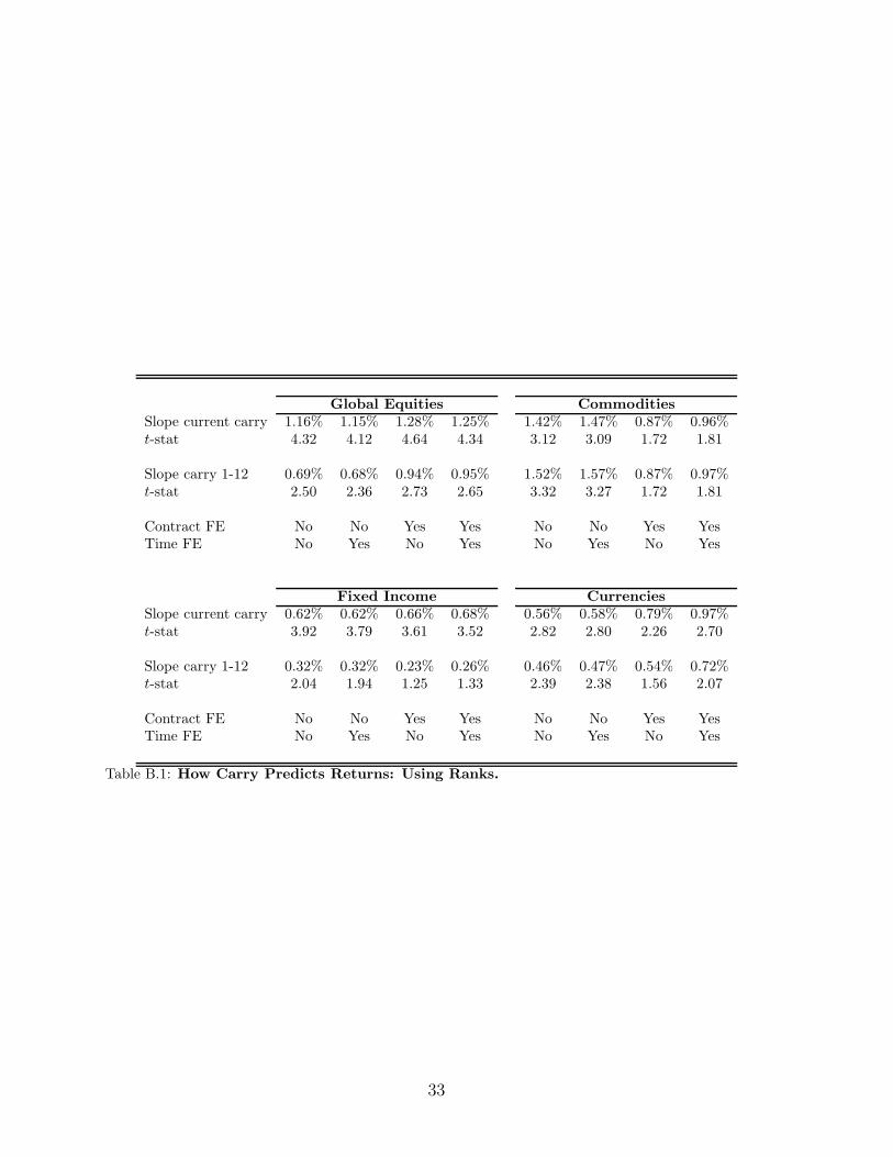
Global Equities Commodities

Slope current carry 1.16% 1.15% 1.28% 1.25% 1.42% 1.47% 0.87% 0.96%t-stat 4.32 4.12 4.64 4.34 3.12 3.09 1.72 1.81

Slope carry 1-12 0.69% 0.68% 0.94% 0.95% 1.52% 1.57% 0.87% 0.97%t-stat 2.50 2.36 2.73 2.65 3.32 3.27 1.72 1.81

Contract FE No No Yes Yes No No Yes YesTime FE No Yes No Yes No Yes No Yes

Fixed Income Currencies

Slope current carry 0.62% 0.62% 0.66% 0.68% 0.56% 0.58% 0.79% 0.97%t-stat 3.92 3.79 3.61 3.52 2.82 2.80 2.26 2.70

Slope carry 1-12 0.32% 0.32% 0.23% 0.26% 0.46% 0.47% 0.54% 0.72%t-stat 2.04 1.94 1.25 1.33 2.39 2.38 1.56 2.07

Contract FE No No Yes Yes No No Yes YesTime FE No Yes No Yes No Yes No Yes

Table B.1: How Carry Predicts Returns: Using Ranks.

33

References

Acharya, Viral, Lars Lochstoer, and Tarun Ramadorai, 2010, Limits to arbitrage and

hedging: Evidence from commodity markets, Working paper.

Acharya, Viral V., and Lasse Heje Pedersen, 2005, Asset pricing with liquidity risk,

Journal of Financial Economics 77, 375–410.

Asness, Cliff, Tobias Moskowitz, and Lasse Heje Pedersen, 2010, Value and momentum

everywhere, Working Paper.

Bacchetta, Philippe, and Eric van Wincoop, 2010, Infrequent portfolio decisions: A

solution to the forward discount puzzle, American Economic Review 100, 837–869.

Bailey, Warren, and K. C. Chan, 1993, Macroeconomic influences and the variability of

the commodity futures basis, Journal of Finance 48, 555–573.

Bansal, Ravi, and Amir Yaron, 2004, Risks for the long-run: A potential resolution of

asset pricing puzzles, Journal of Finance 59, 1481–1509.

Barr, David G., and Richard Priestley, 2004, Expected returns, risk and the integration

of international bond markets, Journal of International Money and Finance 23, 71–97.

Bessembinder, Hendrik, 1992, Msystematic risk, hedging pressure, and risk premiums in

futures markets, Review of Financial Studies 4, 637–667.

Binsbergen, Jules van, Michael W. Brandt, and Ralph S.J. Koijen, 2010, On the timing

and pricing of dividends, American Economic Review, forthcoming.

Binsbergen, Jules van, Wouter Hueskes, Ralph S.J. Koijen, and Evert B. Vrugt, 2010,

Equity yields, Working Paper: Northwestern University and University of Chicago.

Brunnermeier, Markus K., Stefan Nagel, and Lasse H. Pedersen, 2008, Carry Trades and

Currency Crashes, NBER Macroeconomics Annual 23, 313–348.

Brunnermeier, Markus .K., and Lasse H. Pedersen, 2009, Market Liquidity and Funding

Liquidity, Review of Financial Studies 22, 2201–2238.

Burnside, Craig, Martin Eichenbaum, Isaac Kleshchelski, and Sergio Rebelo, 2006, The

returns to currency speculation, Working Paper.

34

Campbell, John Y., and John H. Cochrane, 1999, By force of habit: A consumption-

based explanation of aggregate stock market behavior, Journal of Political Economy

107, 205–251.

Casassus, J., and P. Collin-Dufresne, 2005, Stochastic convenience yield implied from

commodity futures and interest rates, The Journal of Finance 60, 2283–2331.

Chan, Louis K. C., Yasushi Hamao, and Josef Lakonishok, 1991, Fundamentals and stock

returns in japan, Journal of Finance 46, 1739–1764.

Engel, Charles, 1996, The forward discount anomaly and the risk permium: A survey of

recent evidence, Journal of Empirical Finance 3, 123–192.

Erb, C.B., and C.R. Harvey, 2006, The strategic and tactical value of commodity futures,

Financial Analysts Journal pp. 69–97.

Fama, Eugene F., 1984, Forward and spot exchange rates, Journal of Monetary Economics

14, 319–338.

, and Kenneth R. French, 1987, Commodity futures prices: Some evidence on

forecast power, premiums, and the theory of storage, Journal of Business 60, 55–73.

, 1998, Value versus growth: The international evidence, Journal of Finance 53,

1975–1999.

, 2011, Size, value, and momentum in international stock returns, Working Paper.

Farhi, Emmanuel, and Xavier Gabaix, 2008, Rare disasters and exchange rates, working

paper.

Froot, Kenneth A., and Richard H. Thaler, 1990, Anomalies: Foreign exchange, Journal

of Economic Perspectives 4, 179–192.

Gabaix, Xavier, 2009, Variable rare disasters: An exactly solved framework for ten puzzles

in macro-finance, Working paper, NYU.

Garleanu, Nicolae, and Lasse Heje Pedersen, 2011, Margin-Based Asset Pricing and

Deviations from the Law of One Price, Review of Financial Studies 24, 1980–2022.

Gorton, Gary, Fumio Hayashi, and Geert Rouwenhorst, 2007, The fundamentals of

commodity futures returns, Working paper.

35

Griffin, John M., 2002, Are the fama and french factors global or country specific?, Review

of Financial Studies 15, 783–803.

, Xiuqing Ji, and J. Spencer Martin, 2003, Momentum investing and business

cycle risk: Evidence from pole to pole, Journal of Finance 58, 2515–2547.

Hong, Harrison, and Mothiro Yogo, 2010, What does futures market interest tell us about

the macroeconomy and asset prices?, Working paper.

Hou, Kewei, G. Andrew Karolyi, and Bong Chan Kho, 2010, What factors drive global

stock returns?, Working Paper.

Ilmanen, Antti, 1995, Time-varying expected returns in international bond markets,

Journal of Finance 50, 481–506.

Lewis, K.K., 1995, Puzzles in international financial markets, in Gene M. Grossman, and

Kenneth Rogoff, ed.: Handbook of International Economics vol. 3 (North Holland:

Amsterdam) Chap. 37.

Lucas, Robert, 1978, Asset prices in an exchange economy, Econometrica 46, 1429–1446.

Lustig, Hanno, Nicholas Roussanov, and Adrien Verdelhan, 2010, Countercyclical

currency risk premia, Working Paper.

Lustig, Hanno, and Adrien Verdelhan, 2007, The cross-section of foreign currency risk

premia and us consumption growth risk, American Economic Review 97, 89–117.

Meese, R.A., and K. Rogoff, 1983, Empirical exchange rate models of the seventies:: Do

they fit out of sample?, Journal of international economics 14, 3–24.

Moskowitz, Tobias, Yao Hua Ooi, and Lasse Heje Pedersen, 2010, Time series momentum,

Working Paper.

Moskowitz, Tobias J., Yao Hua Ooi, and Lasse Heje Pedersen, 2012, Time series

momentum, Journal of Financial Economics, forthcoming.

Rouwenhorst, K. Geert, 1998, International momentum strategies, Journal of Finance 53,

267–284.

Szymanowska, Marta, Frans de Roon, Theo E. Nijman, and Rob van den Goorbergh, 2011,

An anatomy of commodity futures risk premia, Working Paper: Erasmus University.

36

Tang, Ke, and Wei Xiong, 2010, Index investment and financialization of commodities,

Working paper.

Wachter, Jessica A., 2010, Can time-varying risk of rare disasters explain aggregate stock

market volatility?, Working Paper.

Yang, Fan, 2011, Investment shocks and the commodity basis spread, Working Paper:

University of Minnesota.

37

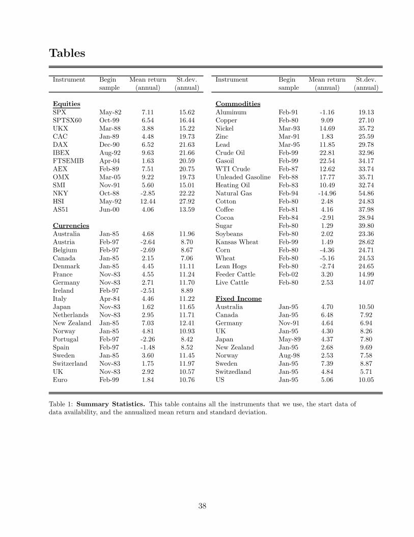
Tables

Instrument Begin Mean return St.dev. Instrument Begin Mean return St.dev.sample (annual) (annual) sample (annual) (annual)

Equities Commodities

SPX May-82 7.11 15.62 Aluminum Feb-91 -1.16 19.13SPTSX60 Oct-99 6.54 16.44 Copper Feb-80 9.09 27.10UKX Mar-88 3.88 15.22 Nickel Mar-93 14.69 35.72CAC Jan-89 4.48 19.73 Zinc Mar-91 1.83 25.59DAX Dec-90 6.52 21.63 Lead Mar-95 11.85 29.78IBEX Aug-92 9.63 21.66 Crude Oil Feb-99 22.81 32.96FTSEMIB Apr-04 1.63 20.59 Gasoil Feb-99 22.54 34.17AEX Feb-89 7.51 20.75 WTI Crude Feb-87 12.62 33.74OMX Mar-05 9.22 19.73 Unleaded Gasoline Feb-88 17.77 35.71SMI Nov-91 5.60 15.01 Heating Oil Feb-83 10.49 32.74NKY Oct-88 -2.85 22.22 Natural Gas Feb-94 -14.96 54.86HSI May-92 12.44 27.92 Cotton Feb-80 2.48 24.83AS51 Jun-00 4.06 13.59 Coffee Feb-81 4.16 37.98

Cocoa Feb-84 -2.91 28.94Currencies Sugar Feb-80 1.29 39.80Australia Jan-85 4.68 11.96 Soybeans Feb-80 2.02 23.36Austria Feb-97 -2.64 8.70 Kansas Wheat Feb-99 1.49 28.62Belgium Feb-97 -2.69 8.67 Corn Feb-80 -4.36 24.71Canada Jan-85 2.15 7.06 Wheat Feb-80 -5.16 24.53Denmark Jan-85 4.45 11.11 Lean Hogs Feb-80 -2.74 24.65France Nov-83 4.55 11.24 Feeder Cattle Feb-02 3.20 14.99Germany Nov-83 2.71 11.70 Live Cattle Feb-80 2.53 14.07Ireland Feb-97 -2.51 8.89Italy Apr-84 4.46 11.22 Fixed Income

Japan Nov-83 1.62 11.65 Australia Jan-95 4.70 10.50Netherlands Nov-83 2.95 11.71 Canada Jan-95 6.48 7.92New Zealand Jan-85 7.03 12.41 Germany Nov-91 4.64 6.94Norway Jan-85 4.81 10.93 UK Jan-95 4.30 8.26Portugal Feb-97 -2.26 8.42 Japan May-89 4.37 7.80Spain Feb-97 -1.48 8.52 New Zealand Jan-95 2.68 9.69Sweden Jan-85 3.60 11.45 Norway Aug-98 2.53 7.58Switzerland Nov-83 1.75 11.97 Sweden Jan-95 7.39 8.87UK Nov-83 2.92 10.57 Switzedland Jan-95 4.84 5.71Euro Feb-99 1.84 10.76 US Jan-95 5.06 10.05

Table 1: Summary Statistics. This table contains all the instruments that we use, the start data ofdata availability, and the annualized mean return and standard deviation.

38

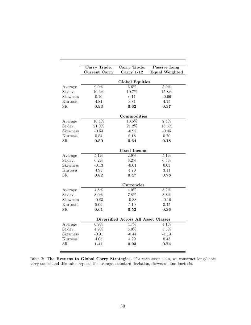
Carry Trade: Carry Trade: Passive Long:

Current Carry Carry 1-12 Equal Weighted

Global Equities

Average 9.9% 6.6% 5.9%St.dev. 10.6% 10.7% 15.8%Skewness 0.10 0.11 -0.66Kurtosis 4.81 3.81 4.15SR 0.93 0.62 0.37

Commodities

Average 10.4% 13.5% 2.4%St.dev. 21.0% 21.2% 13.5%Skewness -0.53 -0.92 -0.45Kurtosis 5.54 6.18 5.70SR 0.50 0.64 0.18

Fixed Income

Average 5.1% 2.9% 5.1%St.dev. 6.2% 6.2% 6.4%Skewness -0.13 -0.01 0.03Kurtosis 4.95 4.70 3.11SR 0.82 0.47 0.78

Currencies

Average 4.8% 4.0% 3.2%St.dev. 8.0% 7.8% 8.8%Skewness -0.83 -0.88 -0.10Kurtosis 5.09 5.19 3.45SR 0.61 0.52 0.36

Diversified Across All Asset Classes

Average 6.9% 4.7% 4.1%St.dev. 4.9% 5.0% 5.5%Skewness -0.31 -0.44 -1.13Kurtosis 4.05 4.29 8.43SR 1.41 0.93 0.74

Table 2: The Returns to Global Carry Strategies. For each asset class, we construct long/shortcarry trades and this table reports the average, standard deviation, skewness, and kurtosis.

39

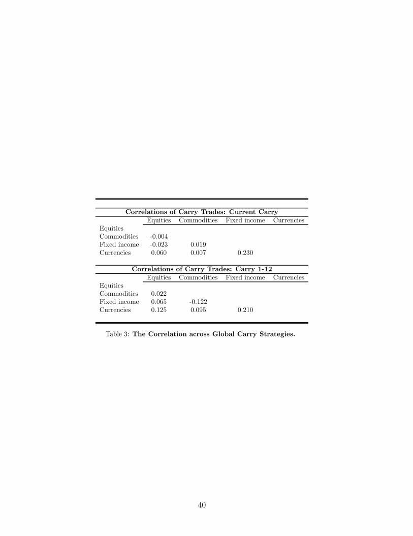
Correlations of Carry Trades: Current Carry

Equities Commodities Fixed income CurrenciesEquitiesCommodities -0.004Fixed income -0.023 0.019Currencies 0.060 0.007 0.230

Correlations of Carry Trades: Carry 1-12

Equities Commodities Fixed income CurrenciesEquitiesCommodities 0.022Fixed income 0.065 -0.122Currencies 0.125 0.095 0.210

Table 3: The Correlation across Global Carry Strategies.

40

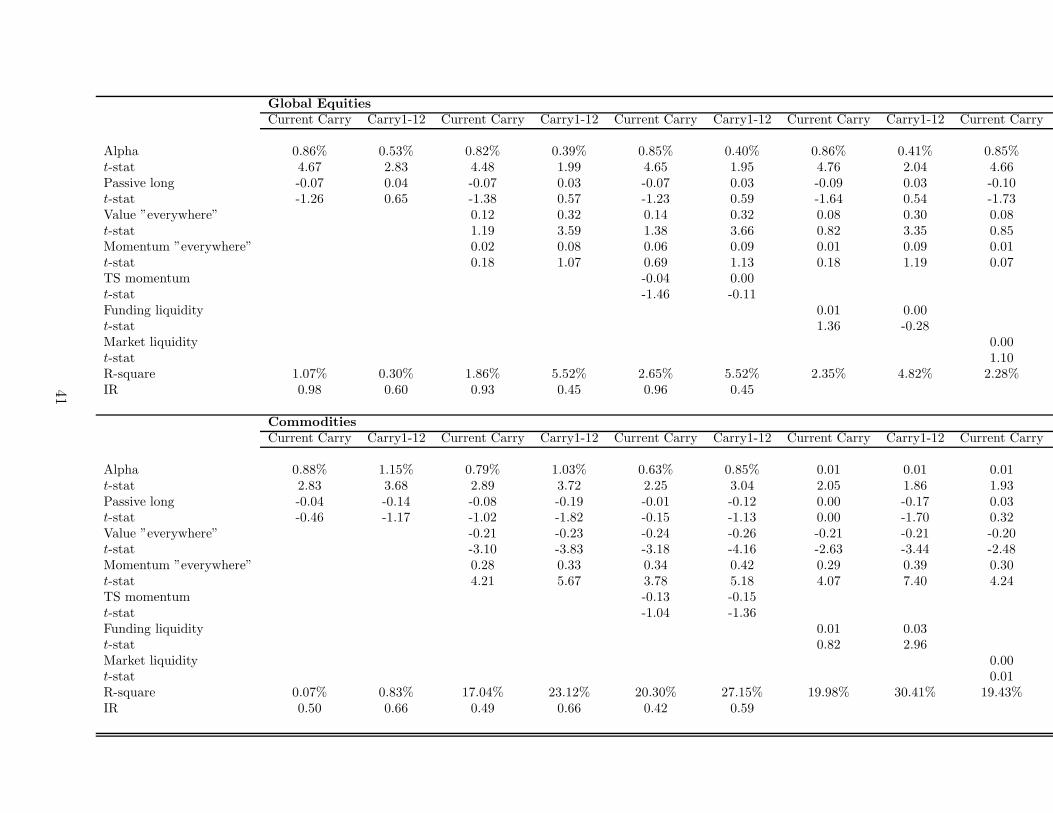
Global Equities

Current Carry Carry1-12 Current Carry Carry1-12 Current Carry Carry1-12 Current Carry Carry1-12 Current Carry

Alpha 0.86% 0.53% 0.82% 0.39% 0.85% 0.40% 0.86% 0.41% 0.85%t-stat 4.67 2.83 4.48 1.99 4.65 1.95 4.76 2.04 4.66Passive long -0.07 0.04 -0.07 0.03 -0.07 0.03 -0.09 0.03 -0.10t-stat -1.26 0.65 -1.38 0.57 -1.23 0.59 -1.64 0.54 -1.73Value ”everywhere” 0.12 0.32 0.14 0.32 0.08 0.30 0.08t-stat 1.19 3.59 1.38 3.66 0.82 3.35 0.85Momentum ”everywhere” 0.02 0.08 0.06 0.09 0.01 0.09 0.01t-stat 0.18 1.07 0.69 1.13 0.18 1.19 0.07TS momentum -0.04 0.00t-stat -1.46 -0.11Funding liquidity 0.01 0.00t-stat 1.36 -0.28Market liquidity 0.00t-stat 1.10R-square 1.07% 0.30% 1.86% 5.52% 2.65% 5.52% 2.35% 4.82% 2.28%IR 0.98 0.60 0.93 0.45 0.96 0.45

Commodities

Current Carry Carry1-12 Current Carry Carry1-12 Current Carry Carry1-12 Current Carry Carry1-12 Current Carry

Alpha 0.88% 1.15% 0.79% 1.03% 0.63% 0.85% 0.01 0.01 0.01t-stat 2.83 3.68 2.89 3.72 2.25 3.04 2.05 1.86 1.93Passive long -0.04 -0.14 -0.08 -0.19 -0.01 -0.12 0.00 -0.17 0.03t-stat -0.46 -1.17 -1.02 -1.82 -0.15 -1.13 0.00 -1.70 0.32Value ”everywhere” -0.21 -0.23 -0.24 -0.26 -0.21 -0.21 -0.20t-stat -3.10 -3.83 -3.18 -4.16 -2.63 -3.44 -2.48Momentum ”everywhere” 0.28 0.33 0.34 0.42 0.29 0.39 0.30t-stat 4.21 5.67 3.78 5.18 4.07 7.40 4.24TS momentum -0.13 -0.15t-stat -1.04 -1.36Funding liquidity 0.01 0.03t-stat 0.82 2.96Market liquidity 0.00t-stat 0.01R-square 0.07% 0.83% 17.04% 23.12% 20.30% 27.15% 19.98% 30.41% 19.43%IR 0.50 0.66 0.49 0.66 0.42 0.59

41

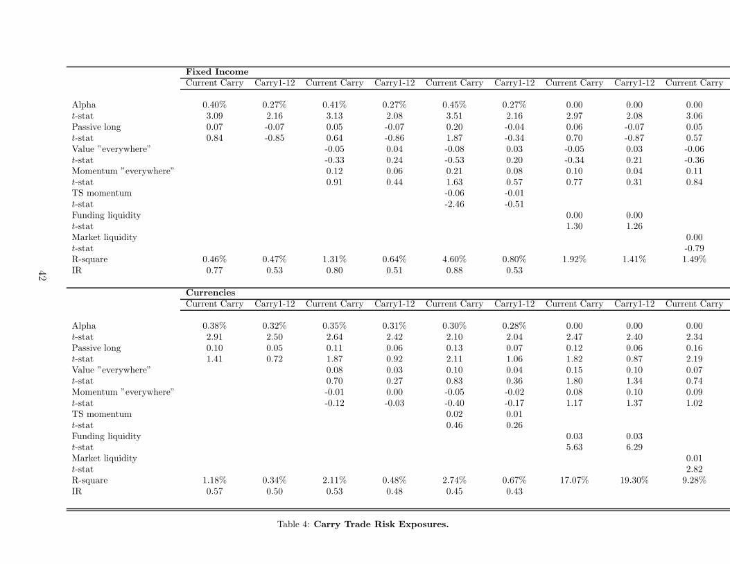
Fixed Income

Current Carry Carry1-12 Current Carry Carry1-12 Current Carry Carry1-12 Current Carry Carry1-12 Current Carry

Alpha 0.40% 0.27% 0.41% 0.27% 0.45% 0.27% 0.00 0.00 0.00t-stat 3.09 2.16 3.13 2.08 3.51 2.16 2.97 2.08 3.06Passive long 0.07 -0.07 0.05 -0.07 0.20 -0.04 0.06 -0.07 0.05t-stat 0.84 -0.85 0.64 -0.86 1.87 -0.34 0.70 -0.87 0.57Value ”everywhere” -0.05 0.04 -0.08 0.03 -0.05 0.03 -0.06t-stat -0.33 0.24 -0.53 0.20 -0.34 0.21 -0.36Momentum ”everywhere” 0.12 0.06 0.21 0.08 0.10 0.04 0.11t-stat 0.91 0.44 1.63 0.57 0.77 0.31 0.84TS momentum -0.06 -0.01t-stat -2.46 -0.51Funding liquidity 0.00 0.00t-stat 1.30 1.26Market liquidity 0.00t-stat -0.79R-square 0.46% 0.47% 1.31% 0.64% 4.60% 0.80% 1.92% 1.41% 1.49%IR 0.77 0.53 0.80 0.51 0.88 0.53

Currencies

Current Carry Carry1-12 Current Carry Carry1-12 Current Carry Carry1-12 Current Carry Carry1-12 Current Carry

Alpha 0.38% 0.32% 0.35% 0.31% 0.30% 0.28% 0.00 0.00 0.00t-stat 2.91 2.50 2.64 2.42 2.10 2.04 2.47 2.40 2.34Passive long 0.10 0.05 0.11 0.06 0.13 0.07 0.12 0.06 0.16t-stat 1.41 0.72 1.87 0.92 2.11 1.06 1.82 0.87 2.19Value ”everywhere” 0.08 0.03 0.10 0.04 0.15 0.10 0.07t-stat 0.70 0.27 0.83 0.36 1.80 1.34 0.74Momentum ”everywhere” -0.01 0.00 -0.05 -0.02 0.08 0.10 0.09t-stat -0.12 -0.03 -0.40 -0.17 1.17 1.37 1.02TS momentum 0.02 0.01t-stat 0.46 0.26Funding liquidity 0.03 0.03t-stat 5.63 6.29Market liquidity 0.01t-stat 2.82R-square 1.18% 0.34% 2.11% 0.48% 2.74% 0.67% 17.07% 19.30% 9.28%IR 0.57 0.50 0.53 0.48 0.45 0.43

Table 4: Carry Trade Risk Exposures.

42

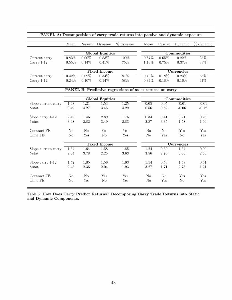
PANEL A: Decomposition of carry trade returns into passive and dynamic exposure

Mean Passive Dynamic % dynamic Mean Passive Dynamic % dynamic

Global Equities Commodities

Current carry 0.83% 0.00% 0.83% 100% 0.87% 0.65% 0.22% 25%Carry 1-12 0.55% 0.14% 0.41% 75% 1.13% 0.75% 0.37% 33%

Fixed Income Currencies

Current carry 0.42% 0.09% 0.34% 81% 0.40% 0.18% 0.23% 58%Carry 1-12 0.24% 0.10% 0.14% 58% 0.34% 0.18% 0.16% 47%

PANEL B: Predictive regressions of asset returns on carry

Global Equities Commodities

Slope current carry 1.48 1.21 1.53 1.25 0.05 0.05 -0.01 -0.01t-stat 3.49 4.27 3.45 4.29 0.56 0.59 -0.06 -0.12

Slope carry 1-12 2.42 1.46 2.89 1.76 0.34 0.41 0.21 0.26t-stat 3.48 2.82 3.49 2.83 2.87 3.35 1.58 1.94

Contract FE No No Yes Yes No No Yes YesTime FE No Yes No Yes No Yes No Yes

Fixed Income Currencies

Slope current carry 1.54 1.64 1.58 1.85 1.24 0.69 1.54 0.90t-stat 2.64 3.78 2.25 3.63 3.56 2.70 3.03 2.60

Slope carry 1-12 1.52 1.05 1.56 1.03 1.14 0.53 1.48 0.61t-stat 2.43 2.36 2.04 1.93 3.27 1.71 2.75 1.21

Contract FE No No Yes Yes No No Yes YesTime FE No Yes No Yes No Yes No Yes

Table 5: How Does Carry Predict Returns? Decomposing Carry Trade Returns into Static

and Dynamic Components.

43

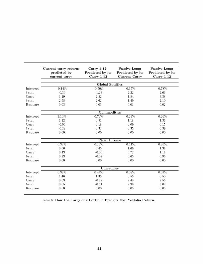
Current carry returns Carry 1-12: Passive Long: Passive Long:

predicted by Predicted by its Predicted by its Predicted by its

current carry Carry 1-12 Current Carry Carry 1-12

Global Equities

Intercept -0.14% -0.50% 0.65% 0.78%t-stat -0.39 -1.23 2.22 2.66Carry 1.29 2.52 1.84 3.38t-stat 2.58 2.62 1.49 2.10R-square 0.03 0.03 0.01 0.02

Commodities

Intercept 1.10% 0.70% 0.23% 0.26%t-stat 1.32 0.51 1.18 1.36Carry -0.06 0.18 0.09 0.15t-stat -0.28 0.32 0.35 0.39R-square 0.00 0.00 0.00 0.00

Fixed Income

Intercept 0.32% 0.26% 0.31% 0.26%t-stat 0.66 0.45 1.66 1.31Carry 0.43 -0.06 0.72 1.11t-stat 0.23 -0.02 0.65 0.96R-square 0.00 0.00 0.00 0.00

Currencies

Intercept 0.39% 0.44% 0.08% 0.07%t-stat 1.46 1.33 0.55 0.50Carry 0.03 -0.22 2.48 2.56t-stat 0.05 -0.31 2.99 3.02R-square 0.00 0.00 0.03 0.03

Table 6: How the Carry of a Portfolio Predicts the Portfolio Return.

44

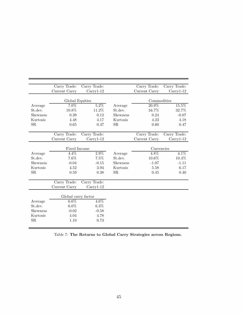
Carry Trade: Carry Trade: Carry Trade: Carry Trade:Current Carry Carry1-12 Current Carry Carry1-12

Global Equities CommoditiesAverage 7.0% 5.2% Average 20.9% 15.5%St.dev. 10.8% 11.2% St.dev. 34.7% 32.7%Skewness 0.39 0.12 Skewness 0.24 -0.07Kurtosis 4.48 4.17 Kurtosis 4.23 4.18SR 0.65 0.47 SR 0.60 0.47

Carry Trade: Carry Trade: Carry Trade: Carry Trade:Current Carry Carry1-12 Current Carry Carry1-12

Fixed Income CurrenciesAverage 4.4% 2.9% Average 4.8% 4.1%St.dev. 7.6% 7.5% St.dev. 10.6% 10.4%Skewness -0.04 -0.15 Skewness -1.07 -1.11Kurtosis 4.52 3.94 Kurtosis 5.58 6.17SR 0.59 0.38 SR 0.45 0.40

Carry Trade: Carry Trade:Current Carry Carry1-12

Global carry factorAverage 6.6% 4.6%St.dev. 6.0% 6.3%Skewness -0.02 -0.58Kurtosis 4.04 4.78SR 1.10 0.73

Table 7: The Returns to Global Carry Strategies across Regions.

45

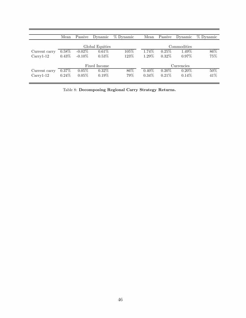
Mean Passive Dynamic % Dynamic Mean Passive Dynamic % Dynamic

Global Equities CommoditiesCurrent carry 0.58% -0.02% 0.61% 105% 1.74% 0.25% 1.49% 86%Carry1-12 0.43% -0.10% 0.53% 123% 1.29% 0.32% 0.97% 75%

Fixed Income CurrenciesCurrent carry 0.37% 0.05% 0.32% 86% 0.40% 0.20% 0.20% 50%Carry1-12 0.24% 0.05% 0.19% 79% 0.34% 0.21% 0.14% 41%

Table 8: Decomposing Regional Carry Strategy Returns.

46

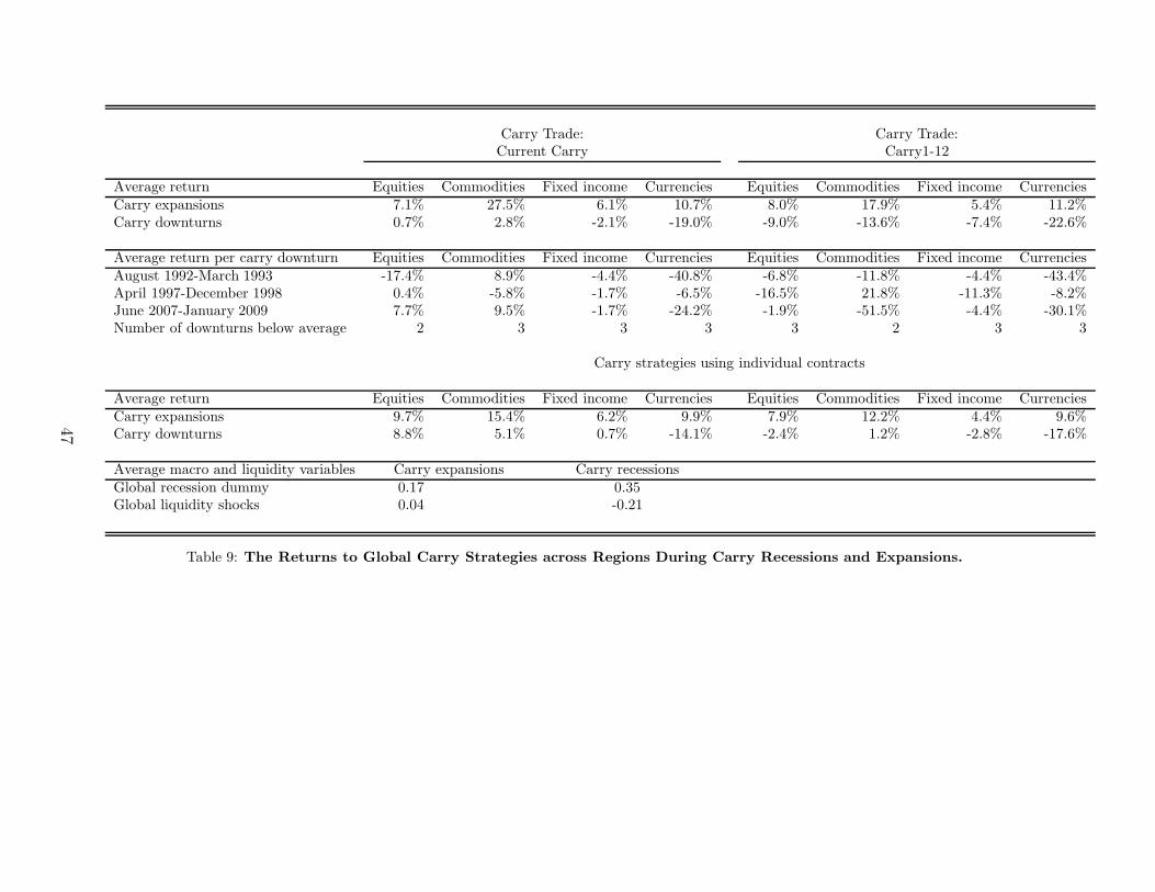
Carry Trade: Carry Trade:Current Carry Carry1-12

Average return Equities Commodities Fixed income Currencies Equities Commodities Fixed income CurrenciesCarry expansions 7.1% 27.5% 6.1% 10.7% 8.0% 17.9% 5.4% 11.2%Carry downturns 0.7% 2.8% -2.1% -19.0% -9.0% -13.6% -7.4% -22.6%

Average return per carry downturn Equities Commodities Fixed income Currencies Equities Commodities Fixed income CurrenciesAugust 1992-March 1993 -17.4% 8.9% -4.4% -40.8% -6.8% -11.8% -4.4% -43.4%April 1997-December 1998 0.4% -5.8% -1.7% -6.5% -16.5% 21.8% -11.3% -8.2%June 2007-January 2009 7.7% 9.5% -1.7% -24.2% -1.9% -51.5% -4.4% -30.1%Number of downturns below average 2 3 3 3 3 2 3 3

Carry strategies using individual contracts

Average return Equities Commodities Fixed income Currencies Equities Commodities Fixed income CurrenciesCarry expansions 9.7% 15.4% 6.2% 9.9% 7.9% 12.2% 4.4% 9.6%Carry downturns 8.8% 5.1% 0.7% -14.1% -2.4% 1.2% -2.8% -17.6%

Average macro and liquidity variables Carry expansions Carry recessionsGlobal recession dummy 0.17 0.35Global liquidity shocks 0.04 -0.21

Table 9: The Returns to Global Carry Strategies across Regions During Carry Recessions and Expansions.

47

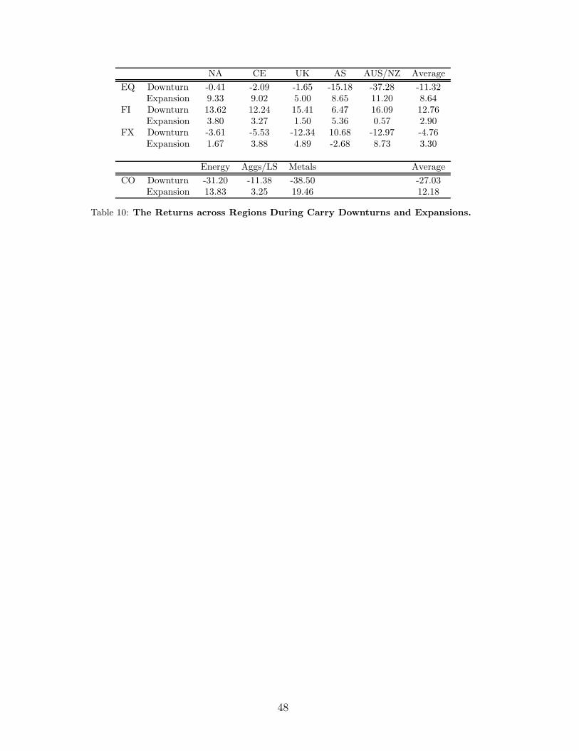
NA CE UK AS AUS/NZ Average

EQ Downturn -0.41 -2.09 -1.65 -15.18 -37.28 -11.32Expansion 9.33 9.02 5.00 8.65 11.20 8.64

FI Downturn 13.62 12.24 15.41 6.47 16.09 12.76Expansion 3.80 3.27 1.50 5.36 0.57 2.90

FX Downturn -3.61 -5.53 -12.34 10.68 -12.97 -4.76Expansion 1.67 3.88 4.89 -2.68 8.73 3.30

Energy Aggs/LS Metals Average

CO Downturn -31.20 -11.38 -38.50 -27.03Expansion 13.83 3.25 19.46 12.18

Table 10: The Returns across Regions During Carry Downturns and Expansions.

48

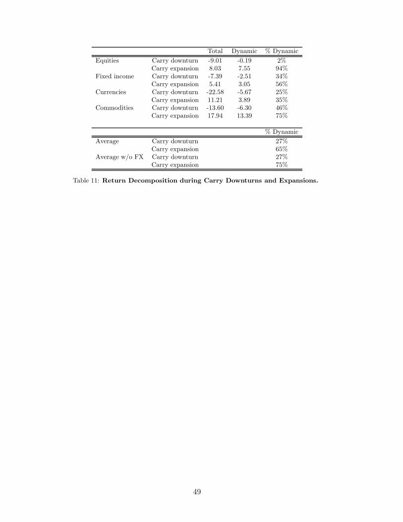
Total Dynamic % Dynamic

Equities Carry downturn -9.01 -0.19 2%Carry expansion 8.03 7.55 94%

Fixed income Carry downturn -7.39 -2.51 34%Carry expansion 5.41 3.05 56%

Currencies Carry downturn -22.58 -5.67 25%Carry expansion 11.21 3.89 35%

Commodities Carry downturn -13.60 -6.30 46%Carry expansion 17.94 13.39 75%

% Dynamic

Average Carry downturn 27%Carry expansion 65%

Average w/o FX Carry downturn 27%Carry expansion 75%

Table 11: Return Decomposition during Carry Downturns and Expansions.

49

Figures

50

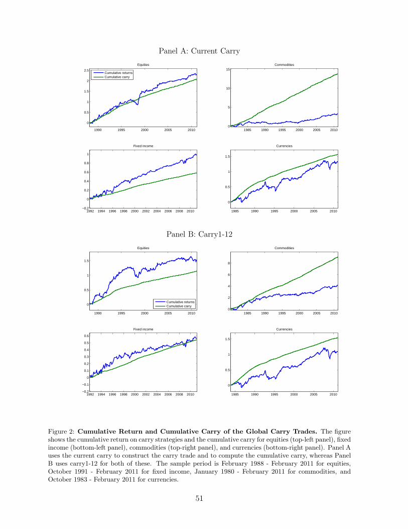
Panel A: Current Carry

1990 1995 2000 2005 2010

0

0.5

1

1.5

2

2.5

Equities

Cumulative returnsCumulative carry

1985 1990 1995 2000 2005 20100

5

10

15Commodities

1992 1994 1996 1998 2000 2002 2004 2006 2008 2010−0.2

0

0.2

0.4

0.6

0.8

1

Fixed income

1985 1990 1995 2000 2005 2010

0

0.5

1

1.5

Currencies

Panel B: Carry1-12

1990 1995 2000 2005 2010

0

0.5

1

1.5

Equities

Cumulative returnsCumulative carry

1985 1990 1995 2000 2005 20100

2

4

6

8

Commodities

1992 1994 1996 1998 2000 2002 2004 2006 2008 2010−0.2

−0.1

0

0.1

0.2

0.3

0.4

0.5

0.6

Fixed income

1985 1990 1995 2000 2005 2010

0

0.5

1

1.5

Currencies

Figure 2: Cumulative Return and Cumulative Carry of the Global Carry Trades. The figureshows the cumulative return on carry strategies and the cumulative carry for equities (top-left panel), fixedincome (bottom-left panel), commodities (top-right panel), and currencies (bottom-right panel). Panel Auses the current carry to construct the carry trade and to compute the cumulative carry, whereas PanelB uses carry1-12 for both of these. The sample period is February 1988 - February 2011 for equities,October 1991 - February 2011 for fixed income, January 1980 - February 2011 for commodities, andOctober 1983 - February 2011 for currencies.

51

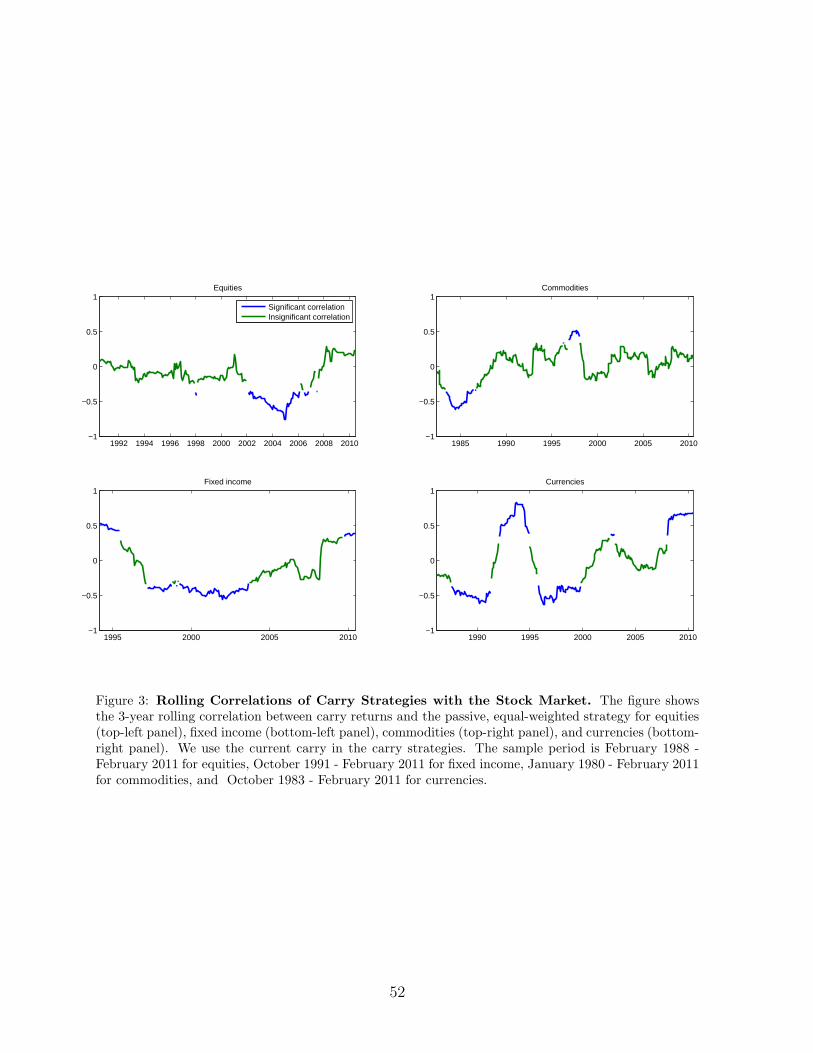
1992 1994 1996 1998 2000 2002 2004 2006 2008 2010−1

−0.5

0

0.5

1Equities

Significant correlationInsignificant correlation

1985 1990 1995 2000 2005 2010−1

−0.5

0

0.5

1Commodities

1995 2000 2005 2010−1

−0.5

0

0.5

1Fixed income

1990 1995 2000 2005 2010−1

−0.5

0

0.5

1Currencies

Figure 3: Rolling Correlations of Carry Strategies with the Stock Market. The figure showsthe 3-year rolling correlation between carry returns and the passive, equal-weighted strategy for equities(top-left panel), fixed income (bottom-left panel), commodities (top-right panel), and currencies (bottom-right panel). We use the current carry in the carry strategies. The sample period is February 1988 -February 2011 for equities, October 1991 - February 2011 for fixed income, January 1980 - February 2011for commodities, and October 1983 - February 2011 for currencies.

52

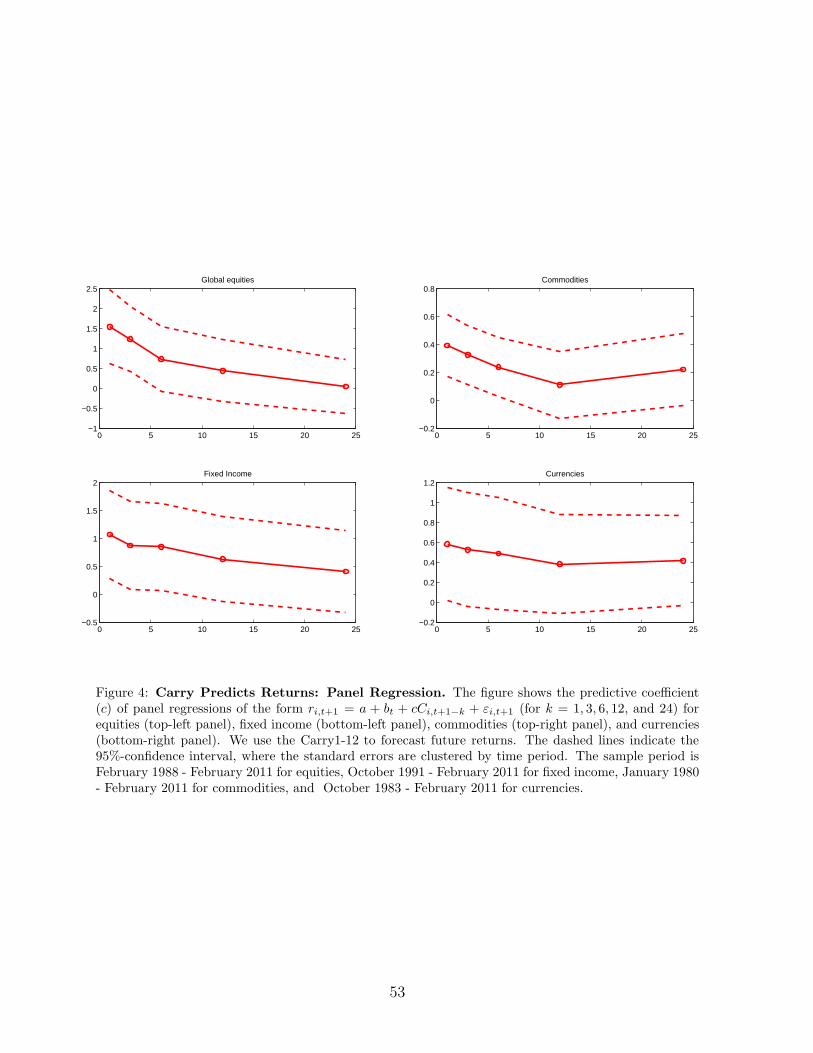
0 5 10 15 20 25−1

−0.5

0

0.5

1

1.5

2

2.5Global equities

0 5 10 15 20 25−0.2

0

0.2

0.4

0.6

0.8Commodities

0 5 10 15 20 25−0.5

0

0.5

1

1.5

2Fixed Income

0 5 10 15 20 25−0.2

0

0.2

0.4

0.6

0.8

1

1.2Currencies

Figure 4: Carry Predicts Returns: Panel Regression. The figure shows the predictive coefficient(c) of panel regressions of the form ri,t+1 = a + bt + cCi,t+1−k + εi,t+1 (for k = 1, 3, 6, 12, and 24) forequities (top-left panel), fixed income (bottom-left panel), commodities (top-right panel), and currencies(bottom-right panel). We use the Carry1-12 to forecast future returns. The dashed lines indicate the95%-confidence interval, where the standard errors are clustered by time period. The sample period isFebruary 1988 - February 2011 for equities, October 1991 - February 2011 for fixed income, January 1980- February 2011 for commodities, and October 1983 - February 2011 for currencies.

53

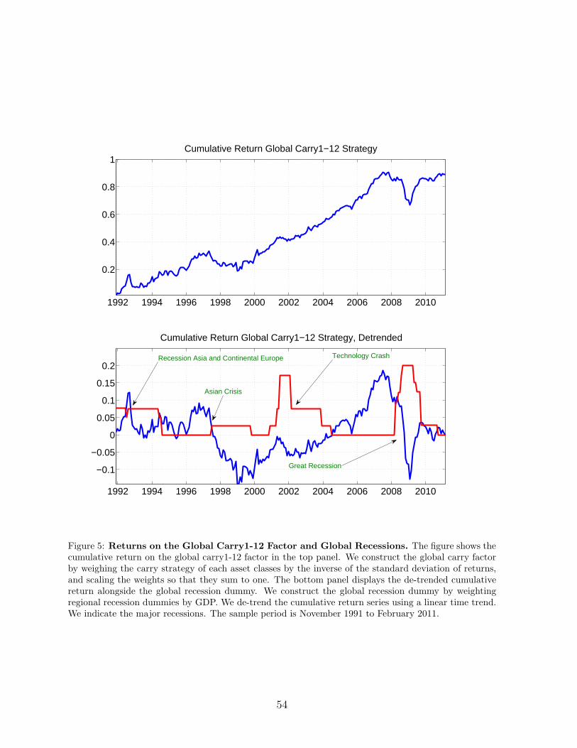
1992 1994 1996 1998 2000 2002 2004 2006 2008 2010

0.2

0.4

0.6

0.8

1Cumulative Return Global Carry1−12 Strategy

1992 1994 1996 1998 2000 2002 2004 2006 2008 2010

−0.1

−0.05

0

0.05

0.1

0.15

0.2

Cumulative Return Global Carry1−12 Strategy, Detrended

Recession Asia and Continental Europe

Asian Crisis

Technology Crash

Great Recession

Figure 5: Returns on the Global Carry1-12 Factor and Global Recessions. The figure shows thecumulative return on the global carry1-12 factor in the top panel. We construct the global carry factorby weighing the carry strategy of each asset classes by the inverse of the standard deviation of returns,and scaling the weights so that they sum to one. The bottom panel displays the de-trended cumulativereturn alongside the global recession dummy. We construct the global recession dummy by weightingregional recession dummies by GDP. We de-trend the cumulative return series using a linear time trend.We indicate the major recessions. The sample period is November 1991 to February 2011.

54

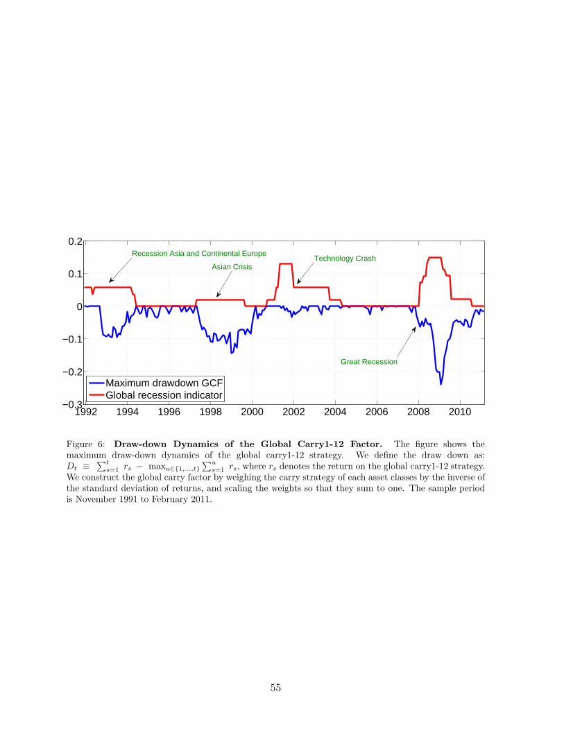
1992 1994 1996 1998 2000 2002 2004 2006 2008 2010−0.3

−0.2

−0.1

0

0.1

0.2

Maximum drawdown GCFGlobal recession indicator

Recession Asia and Continental Europe

Asian Crisis

Great Recession

Technology Crash

Figure 6: Draw-down Dynamics of the Global Carry1-12 Factor. The figure shows themaximum draw-down dynamics of the global carry1-12 strategy. We define the draw down as:Dt ≡

∑t

s=1rs − maxu∈{1,...,t}

∑u

s=1rs, where rs denotes the return on the global carry1-12 strategy.

We construct the global carry factor by weighing the carry strategy of each asset classes by the inverse ofthe standard deviation of returns, and scaling the weights so that they sum to one. The sample periodis November 1991 to February 2011.

55

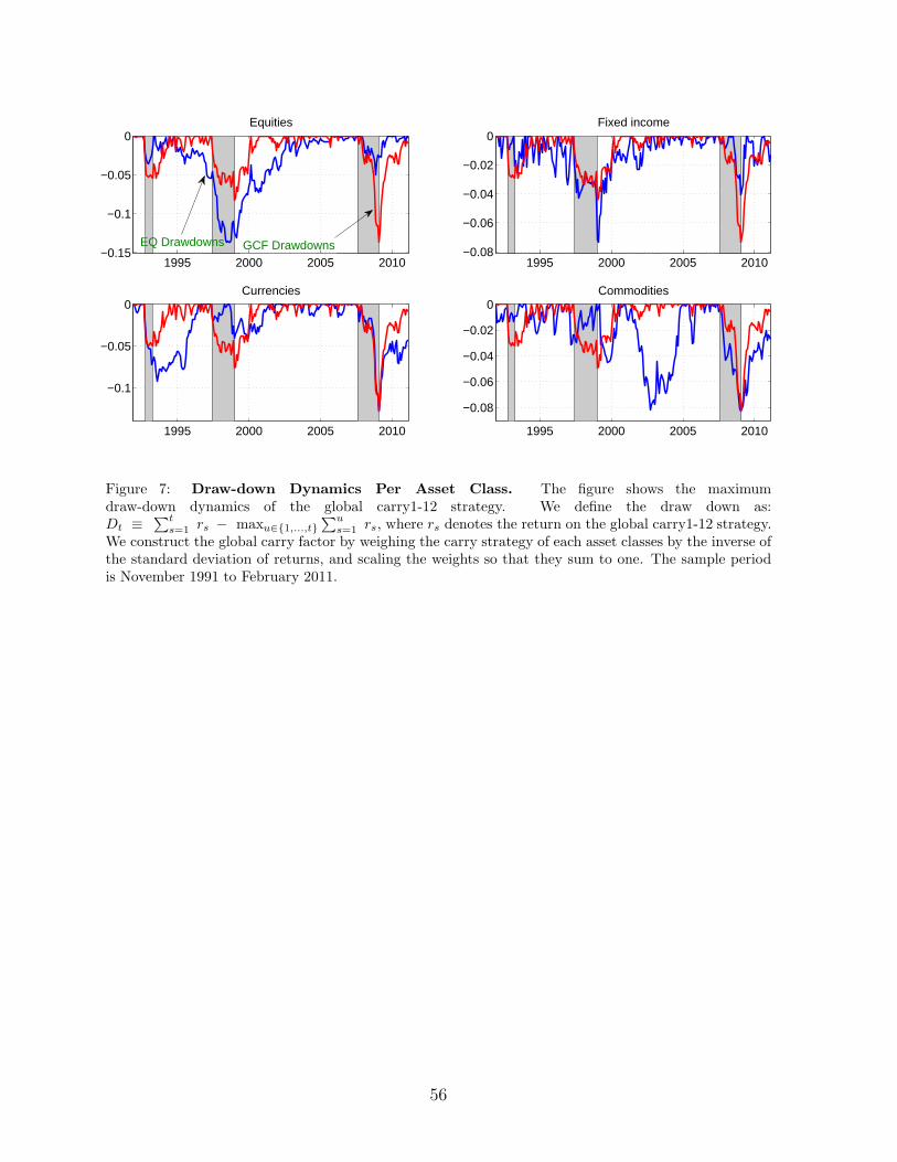
1995 2000 2005 2010−0.15

−0.1

−0.05

0Equities

1995 2000 2005 2010−0.08

−0.06

−0.04

−0.02

0Fixed income

1995 2000 2005 2010

−0.1

−0.05

0Currencies

1995 2000 2005 2010

−0.08

−0.06

−0.04

−0.02

0Commodities

EQ Drawdowns GCF Drawdowns

Figure 7: Draw-down Dynamics Per Asset Class. The figure shows the maximumdraw-down dynamics of the global carry1-12 strategy. We define the draw down as:Dt ≡

∑t

s=1rs − maxu∈{1,...,t}

∑u

s=1rs, where rs denotes the return on the global carry1-12 strategy.

We construct the global carry factor by weighing the carry strategy of each asset classes by the inverse ofthe standard deviation of returns, and scaling the weights so that they sum to one. The sample periodis November 1991 to February 2011.

56