Carpooling and the Economics of Self-Driving Cars∗

Michael Ostrovsky† Michael Schwarz‡

February 12, 2018

Abstract

We study the interplay between autonomous transportation, carpooling, and road pricing.

We discuss how improvements in these technologies, and interactions among them, will affect

transportation markets. Our main results show how to achieve socially efficient outcomes in such

markets, taking into account the costs of driving, road capacity, and commuter preferences. An

important component of the efficient outcome is the socially optimal matching of carpooling

riders. Our approach shows how to set road prices and how to share the costs of driving and

tolls among carpooling riders in a way that implements the efficient outcome.

∗We are grateful to Saurabh Amin, Alexandre Bayen, Ben Edelman, Emir Kamenica, Hal Varian, and LauraWynter for helpful comments and suggestions, and to Suraj Malladi for research assistance. Michael Schwarz wouldlike to disclose that although he is currently at Microsoft, this research was commenced when he was Chief Scientistfor Waze. The views expressed herein are those of the authors and do not necessarily reflect the views of their pastor current employers.

†Stanford Graduate School of Business and NBER; ostrovsky@stanford.edu.‡Microsoft; mschwarz@microsoft.com.

1

1 Introduction

The market for transportation will be transformed by three emerging technologies. Autonomous

driving technology is the most radical of the coming changes, but there are two other emerging

technologies that are less futuristic but potentially no less disruptive. The two other technologies are

technology for time-sensitive tolls that can be charged for each road segment without slowing down

cars and carpooling technology for seamlessly matching cars with multiple passengers. This paper

explores the issue of designing efficient transportation markets powered by these three technologies.

Of course, neither tolls nor carpooling are new. However, the frictions currently associated with

road pricing and carpooling are very high. These frictions are likely to decrease substantially in

the future because of technological improvements.

In the case of tolls, the first generation of the technology involved human toll collectors charging

a payment from each passing car, which had to stop to make the payment. The second (current)

generation of toll technology (like E-ZPass and FasTrak) involves costly hardware at the points

of toll collection. Both technologies are expensive to install and/or run, are thus limited to only

a few major locations, and do not allow toll collection on most road segments. E.g., even in the

major locations where toll collecting systems are installed, such as bridges, the tolls are often

charged only to cars going in one of the two directions, which is not sufficient for efficient traffic

management.1 Generally, implementing toll collection on only a small subset of roads may not be

welfare improving, because traffic flows from those roads may spill over to other streets, worsening

congestion there.

The third (next) generation of toll technology will reduce the cost of physical toll infrastructure

by orders of magnitude, because of advances in GPS, mobile, and other related technologies. These

technologies will make it feasible and practical to charge tolls systemwide, street intersection by

street intersection, allowing regulators to keep roads toll-free during off-peak hours, and to set tolls

high enough to keep traffic flowing during rush hour.2 Moreover, the ability to coordinate tolls on

all the roads in the system together (rather than only on a small subset) will allow regulators to use

the tolls as a powerful tool to optimize systemwide traffic, without worrying about “spillovers” from

paid roads to free ones. Of course, technological constraints are not the only potential barrier to

the adoption of systemwide tolls: commuters may worry about distributional consequences of such

1While adjusting the level of tolls in one direction makes it possible to control the overall flow of traffic, it doesnot allow the regulator to charge time-sensitive tolls in the opposite direction, and thus does not allow to spreadtraffic in that direction over time in an efficient pattern. To give just one example illustrating the high costs of thecurrent technology, in 2007 the U.S. federal government earmarked over one billion dollars for installing a handful oftolls in just five pilot metropolitan areas (“Cities to Split $1.1 Billion For Traffic Proposals,” the Wall Street Journal,August 14, 2007, https://www.wsj.com/articles/SB118713672357497944).

2Satellite-based systems are already in use in several European countries, where they are used to charge tolls ontrucks for road usage. In 2016, the Land Transport Authority of Singapore announced plans to implement a satellite-based toll system for all motorists by year 2020 (“LTA to roll out next-generation ERP from 2020, NCS-MHI to buildsystem for $556m,” the Straits Times, February 25, 2016, http://www.straitstimes.com/singapore/transport/ncs-mhi-to-build-islandwide-satellite-based-erp-for-556m).

2

tolls,3 or about not benefiting from the toll revenue collected by the government.4 As we explain in

Section 2.3, introducing systemwide tolls in the presence of frictionless carpooling technology helps

substantially alleviate these concerns: the two technologies are complementary.

Carpooling is of course also an old “technology,” with a potentially large upside: putting two

or three commuters in a car, instead of having them drive solo, would cut the number of cars

on the road and the cost of transportation in half. Various government initiatives have promoted

carpooling for over half a century, going back to World War II. Yet it still not widely used: according

to the US Census Bureau, only around 9.3% of commuters in the US carpooled to work, compared

to 76.4% who drove alone.5 Why will the future be different from the past? The answer is, again,

technological progress. Perfect carpool partners travel along similar routes at similar times. For

many people, there are many compatible carpool partners—however, these carpool partners change

day to day, because schedules change. Until recently, it was too hard to find a good carpool partner,

at least without advance planning, and too inconvenient to coordinate with him or her. This is

starting to change. New mobile phone apps (e.g., Waze Carpool and Scoop) automate the process

of finding suitable carpool matches with short detours and compatible travel times, and also keep

track of user reputation, preferences, and patterns, and make it seamless for passengers to reimburse

drivers for part of travel costs.6 The products are still in their infancy, available only in limited

geographic areas, but they clearly demonstrate the potential of technology to substantially lower

the frictions associated with carpooling, especially as the technology matures and the network of

commuters who use it grows. So even if the rest of the technological landscape remained unchanged,

the barriers to carpooling would drop, making it more attractive. But viewing technological progress

in carpooling in isolation would present an incomplete picture of its potential.

In Section 2, we argue that there are strong interdependencies between improvements in the

three technologies we mentioned: autonomous transportation, road pricing, and carpooling. Au-

tonomous transportation makes both road pricing and carpooling more convenient and attractive.

Road pricing and carpooling reinforce each other: the former makes the latter more attractive,

and vice versa. These observations raise a variety of questions about the efficient design of trans-

portation in light of these technological improvements and interactions among them. How should

road prices be set? How should carpooling groups be determined? How much should each of the

carpooling passengers pay (e.g., if one passenger is in the car for only a part of the ride, while

another passenger is in the car for the whole ride—but the car had to make a small detour to

3E.g., in response to a proposal to introduce toll lanes on highway 580 in Orange County, state Assemblyman AllanMansoor commented, “If you put toll lanes in, it’s a money grab. Who can afford $10 to $15? Seniors can’t affordit. Low-income families cannot afford it.” (http://abc7.com/news/politicians-oppose-oc-405-fwy-toll-lanes/234209/)

4In which case they may not benefit from having the tolls. E.g., in Vickrey’s (1969) canonical example, (homo-geneous) drivers are indifferent between paying efficient tolls and waiting in traffic: they simply pay in dollars whatthey used to pay in time. The increase in social welfare comes solely from the fact that the time in traffic is a purewaste, while the collected tolls become government revenue. If the revenue is not used to benefit the drivers in anyway, then their welfare is not improved.

5https://factfinder.census.gov/bkmk/table/1.0/en/ACS/16 5YR/S0801/0100000US6https://www.mercurynews.com/2017/01/03/road-warriors-unite-carpooling-apps-wont-save-the-planet-but-

may-help-us-save-each-other/

3

pick up the first passenger)? How should carpooling interact with road pricing (e.g., how should

tolls paid by passengers depend on the number of riders in the car)? Our modeling framework in

Section 3 is designed to address these questions.

The framework blends together ideas from coalition formation games (riders form coalitions to

carpool and share costs) and competitive equilibrium (road prices are set at the level that clears

the market). The framework naturally incorporates interactions between the two components: tolls

impact which carpooling coalitions get formed; in turn, the carpooling coalition formation process

impacts the demand for roads. Our main results in Sections 3.1 and 3.2 show how to achieve

socially efficient outcomes in such markets, taking into account the costs of driving, road capacity,

and commuter preferences. An important component of the efficient outcome is the socially optimal

matching of carpooling riders. Our approach shows how to set road prices and how to share the

costs of driving and tolls among carpooling riders in a way that implements the efficient outcome.

We find that efficient market design for this setting can be “decomposed” into (i) road pricing by

the road authorities (where road segments have positive prices only when they are at capacity, and

are free otherwise) and (ii) unconstrained coalition formation in which groups of riders are allowed

to arrange whichever carpooling trips they want, and can split the costs of those trips in any way

they choose. To the best of our knowledge, this is the first paper that jointly characterizes efficient

tolls and efficient carpooling arrangements.

Our main results are established for an economy in which all cars are self-driving. The technical

difference between a world in which all cars are self-driving vs. one in which some or all cars have

human drivers is that carpool matching with self-driving is a one-sided matching problem, while

with regular cars it is a two-sided one. Section 3.3 points out that our results can be adapted to a

world in which some or all cars are conventional.

In Sections 4 and 5 we discuss various assumptions behind our modeling framework, as well

as potential extensions and generalizations. In Section 4, we consider the issue of the potential

economic gains from increased car utilization (as measured by the fraction of time each car is on

the road). Perhaps surprisingly, these gains turn out to be relatively small—and, in particular,

much smaller than the potential gains from increased utilization of seats within a car (by arranging

carpools with multiple passengers traveling in the same car). This observation informs our mod-

eling framework, specifically, the assumptions that the physical cost of a trip depends only on the

characteristics of that trip, and that for a self-driving car, there is no cost of waiting between trips.

Section 5 concludes with a discussion of other issues related to our model and potential extensions.

2 Technological Interactions

In this section, we discuss the interactions between the three emerging technologies mentioned

in the introduction: autonomous transportation, frictionless carpooling, and improved road pricing.

This discussion explains why a transportation market powered by these technologies needs to be

studied in a unified framework. The framework itself is presented in Section 3. A reader interested

4

Self-DrivingCars

CarpoolingTolls

InformationTechnology

Figure 1: Technological influences

in our formal analysis can skip directly to that section.

Figure 1 illustrates influences between the technologies. The overall progress in information

technology makes self-driving cars feasible, and, as discussed in the introduction, also brings about

dramatic improvements in carpooling and road pricing. Autonomous transportation technology, in

turn, makes carpooling and road pricing even more attractive, as we discuss in Sections 2.1 and

2.2. Finally, as we discuss in Section 2.3, next-generation carpooling and road pricing technologies

are highly complementary and make each other more attractive.

2.1 The influence of autonomous transportation on carpooling

Carpooling can be viewed as a form of public transportation. Currently, the cost of drivers is a

significant component of public transit costs. Because drivers’ time is expensive, public transporta-

tion uses large vehicles that make frequent stops, resulting in slow and often inconvenient service.

By eliminating the cost of drivers’ time, self-driving technology will make public transportation

much cheaper than it is today. Moreover, it will make public transit more convenient by enabling

fewer stops and door-to-door transit at a reasonable cost. Carpooling will become much more

attractive in the world of self-driving cars, blurring the line between solo driving and mass transit.

Below we list various reasons for this impact of autonomous transportation on carpooling.

• No-hassle coordination: regardless of whether or not a rider carpools, the self-driving car

has to know its destination and the possible routes, and so coordinating carpooling does not

require effort on the part of riders.

• It is easy for an automated system to make carpooling matches in real time (i.e., when the

car is already moving) and adjust its route accordingly. For a human driver to accept a ride

request when the car is already moving could be inconvenient or unsafe.

5

• One of the key challenges in creating a carpooling platform is getting to a critical mass

where on-demand carpooling is reliable enough to be practical. With transportation services

powered by self-driving cars, this issue is resolved automatically.

• With several people sharing a ride, it does not have to be the case that the same person is

the first one getting in the car and the last one getting out of it.

• Detours are much less costly: it costs much less to sit in the car as a passenger who is

reading/sleeping/working while the car is making a five-minute detour than to drive during

that time. Essentially, with driving, a five-minute detour costs the driver her regular wage

for that period, while for a passenger in a self-driving car, the cost is lower.

• No need to depend on a potentially unreliable carpool driver.

• No-hassle payments. Social frictions are removed or reduced.

• People are reluctant to carpool in part due to the loss of flexibility: with conventional car-

pooling, the driver needs to commit to a departure time and the passenger needs to be ready

at the agreed-upon time. With real-time carpooling that can be enabled by self-driving cars,

it is possible to offer “asymmetric service”: the first passenger to be picked up pays a small

premium so that the car can wait for her (so she can leave her house at any time during a

certain time window). As the car starts moving, it can pick up other passengers along the

route.

• Consistency of experience. E.g., no need to worry about being matched with an unsafe driver.

• Regular cars are built for families; they are not optimized for carpooling. Self-driving cars

may be built with carpooling use in mind. The seating could then be arranged to maximize

the comfort and privacy of passengers.

2.2 The influence of autonomous transportation on road pricing

With self-driving cars, intelligent systemwide road pricing also becomes more attractive, for the

following reasons.

One reason is the potential equilibrium effect of autonomous transportation on road demand in

the absence of road pricing. Without the need to drive, a rider’s disutility from spending a certain

amount of time in traffic is substantially reduced: she can sleep, work, read, play videogames, and so

on—i.e., engage in many of the same leisure or productive activities that she would otherwise do at

home or at work. While individually attractive, this substantially reduced disutility from spending

time in traffic may lead to highly undesirable equilibrium effects, with riders being much more

willing to take trips during already congested times, and commute over longer distances. Riders

would thus impose even higher negative externalities on others, with ambiguous overall effects on

social welfare, despite the obvious individual benefits of the improved technology. The Tesla CEO

6

Elon Musk expressed a related concern that convenient and affordable autonomous transportation

may lead to increased congestion: “A lot of people think that once you make cars autonomous

that they’ll be able to go faster and that will alleviate congestion and to some degree that will be

true. But . . . the amount of driving that will occur will be much greater with shared autonomy

and actually, traffic will get far worse.”7 In such circumstances, intelligent systemwide road pricing

becomes particularly valuable.

Another reason why self-driving technology makes road pricing more attractive is largely logis-

tical, on the rider side. A passenger of a self-driving car already needs to enter her destination when

she begins the trip, and it is convenient to present road prices at that moment, as well as let her

choose among several options (e.g., a faster route vs. a cheaper one). Similarly, if the passenger’s

departure time is flexible, the system can present her with various options to travel at a lower price

at a different time. In other words, it is convenient to incorporate road pricing directly into the

user interface for autonomous transportation. Note that various carpooling options are also easy

to integrate into the same user interface, allowing the user to choose among various combinations

of options.

The third reason is also logistical, but on the side of technological infrastructure. Since a self-

driving car’s system must already have exact data on what route the car is taking, and at what

time, that data can in principle also be used to compute tolls, at a very low marginal cost relative

to the cost of developing the toll-collection infrastructure from scratch.

2.3 The complementarity between road pricing and carpooling

Finally, there is a strong complementarity between carpooling and road pricing. To illustrate

this complementarity, consider the following simple example based on Vickrey (1969). There is one

congested road, which is a “bottleneck.” Twice as many drivers want to go over that road during

a certain period of time than the road can allow. Without any interventions, we get congestion,

delay, and wasted time. To make the following example as transparent as possible, we assume that

the cost of driving is zero—the only issue is congestion and delay.

• Suppose carpooling becomes very convenient: its disutility (vs. driving solo) is some small

∆ > 0. This has no effect on outcomes, because nobody has an incentive to carpool.

• Suppose there is no carpooling and tolls are set at the socially optimal level. To make the

point particularly stark, suppose also that toll revenues are not spent in ways that benefit

the drivers who pay these tolls. Vickrey (1969) then shows that with homogeneous drivers,

none of the drivers are better off : they simply pay in dollars what they used to pay in time.8

• Now suppose we both have convenient carpooling and set socially optimal tolls. We then fully

relieve congestion, all riders arrive at their most preferred times, and are now much better

7https://electrek.co/2017/05/01/tesla-network-elon-musk-autonomous-ride-sharing-vision/8Society is better off overall, because tolls are an efficient mechanism for raising revenues. A driver’s time in traffic

is a social waste, while toll payments are an efficient transfer. However, as we stated above, drivers are no better offif toll revenues are used by the central authority in a way that does not benefit them.

7

off than they were before—even if all the revenue from tolls is simply destroyed. Moreover,

even if only a fraction of drivers can carpool, they become better off, paying in dollars less

than half of what they used to pay in time.9

Thus, deployed together, intelligent tolls and seamless carpooling operate as a “shock absorber”

for times of peak travel demand: on average, there will be more riders in each car during times of

peak demand than during off-peak hours. Note that both technologies are needed for this shock

absorber to work well, and they reinforce each other. The presence of tolls makes carpooling

more attractive, since it allows riders to share the costs of those tolls and thus pay less and travel

closer to their preferred times—in contrast to the situation with congestion delays and without

tolls, in which carpooling does not reduce any rider’s cost of waiting in traffic. A cost paid in

the form of dollars can be shared among the carpooling riders and thus substantially reduced for

each one of them individually, while a cost paid in the form of time spent in traffic cannot: each

of the carpooling riders “pays” the full amount. Conversely, the presence of convenient, seamless

carpooling makes tolls much more attractive politically, because it gives price-sensitive riders a

feasible way to commute during their preferred times, and can make them substantially better off

even if the revenue from tolls does not benefit them directly.

3 Model and Main Results

In this section, we present our model of a transportation marketplace with autonomous driving,

carpooling, and tolls, and state and prove our main results. In Section 3.1, we present the model

and the first result on efficiency. In Section 3.2, we present an auxiliary, “fractional” model of

transportation, and prove results on existence and efficiency. In Section 3.3, we discuss to what

extent our results are applicable to the world with human drivers.

3.1 Model and Efficiency

There is a finite set of riders m = 1, . . . ,M . There is also a finite set of road segments s =

1, . . . , S. Each road segment s identifies both the physical road segment that can be viewed as an

“indivisible” road unit (e.g., a part of a freeway between two exits) and a specific time. Note that

time is discretized and the same road at two different times is viewed as two distinct road segments.

Each road segment s has an integer capacity qs > 0.

9Hall (2017) discusses the difficulties of allocating toll revenue in ways that make all drivers better off, and alsoraises the question of whether tolls can make all drivers better off even if the revenue from tolls is destroyed. He showsthat putting appropriate tolls on some of the lanes on a congested highway can lead to a Pareto improvement, byrelieving hypercongestion on those lanes and thereby increasing those lanes’ throughput—which would in turn leadto fewer cars and a lower congestion level on the remaining free lanes. However, as Hall (2017) notes, “Obtaining aPareto improvement [. . . ] comes at a cost. By only pricing a portion of the lanes, we leave the other lanes congested,with all the resulting social costs. That said, inasmuch as generating a Pareto improvement makes it politicallyfeasible to implement tolling, then we are trading potential, but unrealized, welfare gains for actual welfare gains.”Our example shows that with carpooling, one may not need to face this trade-off: it may be possible to both obtainthe first-best outcome and generate Pareto improvement for all commuters (relative to the congested status quo),even if all revenue from tolls is destroyed.

8

A trip is a feasible combination of one or more riders and one or more road segments, and

possibly other characteristics (which can encode a wide variety of options: e.g., which rider gets

which seat, what type of car is used, and so on). There is a finite number T of possible trips

t = 1, . . . , T .

Each trip t has a non-negative physical cost c(t) ∈ R associated with it. This cost includes the

physical cost of the resources associated with the trip: gas or electricity used; wear and tear on the

car; etc.

Each rider m has a non-negative valuation for every possible trip t that involves him, vm(t) ∈ R.

We assume that for each rider m, there exists an “outside option” that is represented by a trip

that involves only one rider (m) and no road segments, gives rider m the valuation of zero, and has

the cost of zero. We also assume that for every trip t and every subset of riders involved in trip t,

there exists a trip t′ that involves exactly this subset of riders, involves the same segments as trip

t, has cost c(t′) ≤ c(t), and to every rider m in the subset, gives valuation vm(t′) ≥ vm(t). I.e.,

intuitively, we can drop any rider from a trip without increasing the physical cost of the trip and

without making other riders worse off. Finally, we assume that each trip creates non-negative net

value to its participants:∑

m∈t vm(t)− c(t) ≥ 0, where “m ∈ t” denotes the riders who participate

in trip t.

An assignment is a set of trips A such that each rider is involved in exactly one trip in A (some

of these riders may of course be assigned to their outside option). Assignment A is feasible if for

each road segment s, the number of trips in A that include road segment s does not exceed its

capacity qs.

An observation about our modeling assumptions is in order. By definition, there is no traffic

congestion in a feasible assignment. Obviously, in practice, setting tolls too low (e.g., at zero) can

lead to traffic delays, as cars may have to wait in queues in order to pass through road segments

that lack capacity to meet demand. However, for our purposes, we do not need to model traffic

congestion, much like general equilibrium models do not need to model consumer response to

shortages. Our assumptions say that as long as an assignment is feasible (i.e., the number of cars

on each road segment does not exceed that segment’s capacity), the speed of cars on that road

segment and hence each rider’s utility from a trip does not depend on the number of other cars

using the same road segments. In other words, we implicitly assumed that when traffic congestion

slows down the flow of traffic, the throughput of the road does not increase relative to maximum

throughput that is attainable at speed limit. While this is of course an approximation, it is in

fact largely consistent with the findings from the literature on traffic and road throughput. For

high levels of traffic congestion, overall road throughput is actually reduced relative to throughput

available at higher speeds (this phenomenon is known as “hypercongestion,” see Walters (1961),

who calls this phenomenon “the bottleneck case,” and Small and Chu (2003)). Thus, at high

congestion levels there is no trade-off between speed and throughput. For moderate levels of traffic,

there is a trade-off between the speed of traffic and throughput, however, assuming this trade-off

away is a reasonably accurate approximation of the real world traffic flows, which substantially

9

simplifies the analysis without losing much realism. For example, the highest possible throughput

on highways is attained at speeds that are close to speed limits (Hall, 1996; Varaiya, 2005).10 We

further discuss this assumption in more detail in Section 5.

We now introduce monetary transfers in our model. First, a non-negative vector p ∈ RM

specifies the price paid by each rider m. If a rider m is charged price pm and is assigned to trip tm,

his utility function is quasilinear in money:

Um(tm, pm) = vm(tm)− pm.

Second, a non-negative vector r ∈ RS specifies the tolls imposed by a regulator. Note that tolls are

segment-specific (rather than route-specific): the cost of using a route is equal to the sum of the

tolls for its individual segments. Note also that tolls are imposed on cars rather than on passengers,

and so in particular are not affected by the number of passengers in a car. We discuss the possibility

of more complex tolls that depend on the entire route or on the number of passengers after the

proof of Theorem 1.

An outcome is a triple (A, p, r) that specifies an assignment, the payments made by the riders,

and the tolls imposed by the regulator. An outcome is feasible if the corresponding assignment A

is feasible. An outcome is budget-balanced if the sum of prices paid by the riders for their trips is

greater than or equal to the sum of the total physical costs of those trips and the total tolls on the

road segments involved in those trips. An outcome is stable if no coalition of riders can organize

a trip by themselves (taking the physical cost of that trip and the underlying tolls as given) that

would give each of them a strictly higher utility than what they are getting in the outcome.

The social surplus of assignment A is equal to the sum of the valuations of all the riders from

the trips to which they are assigned in A minus the sum of the costs of the trips in A. Note that

prices p and tolls r do not enter this calculation.

The regulator is interested in maximizing social surplus. Note that feasibility, stability, and

budget-balancedness are not sufficient to guarantee that social surplus is maximized. For instance,

if all tolls are set at a very high level, the outcome that assigns every rider to his outside option and

charges him zero is feasible, stable, and budget-balanced – but is not in general surplus maximizing.

Intuitively, the problem with such a high level of tolls is that it leaves roads underutilized: high

tolls push riders away even from segments that have plenty of capacity. Our last condition rules out

such a possibility. Formally, we say that an outcome is market-clearing if for every road segment

such that the number of trips in A that include it is less than its capacity, the corresponding toll

is equal to zero.

We are now ready to state the first main result of the paper.

10From Varaiya (2005): “There are 26,000 sensors buried under the pavements of California freeways. Every thirtyseconds, those sensors send data to our computers here in Berkeley. The data tell us about the number of cars drivingon that freeway and their speeds at that time. . . . We’ve already learned quite a lot from all those data. For example,we’ve found the error in the old belief that an average speed of 40 to 45 mph maximizes traffic capacity; we nowknow for a fact that maximum capacity occurs at around 60 mph.”

10

Theorem 1 If an outcome (A, pA, rA) is feasible, stable, budget-balanced, and market-clearing,

then assignment A has the highest possible social surplus across all feasible assignments.

Proof. Suppose a different feasible assignment, B, generates a higher social surplus than does

assignment A. Take any trip t in assignment B, and all riders m involved in trip t. Since by

assumption outcome A is stable, this coalition of riders cannot benefit from organizing trip t by

themselves, given prices pA and tolls rA in outcome A. Thus, summing the utilities of all riders

involved in trip t, we get

∑m∈t

(vm(tAm)− pAm

)≥

(∑m∈t

vm(t)

)− c(t)− rA(t), (1)

where tAm denotes the trip in which rider m is involved under assignment A, and, slightly abusing

notation, rA(t) denotes the sum of the tolls on the segments involved in trip t in outcome (A, pA, rA).

Adding up equations (1) across all trips t in assignment B, we get

M∑m=1

vm(tAm)−M∑

m=1

pAm ≥M∑

m=1

vm(tBm)−∑t∈B

c(t)−S∑

s=1

rA(s)kB(s), (2)

where kB(s) denotes how many trips in assignment B use segment s.

Since outcome (A, pA, rA) is by assumption budget-balanced, we have

M∑m=1

pAm ≥∑t∈A

c(t) +S∑

s=1

rA(s)kA(s).

Thus, equation (2) implies that

M∑m=1

vm(tAm)−∑t∈A

c(t)−S∑

s=1

rA(s)kA(s) ≥M∑

m=1

vm(tBm)−∑t∈B

c(t)−S∑

s=1

rA(s)kB(s). (3)

The social surplus of assignment A is equal to∑M

m=1 vm(tAm)−∑

t∈A c(t), while the social surplus

of assignment B is equal to∑M

m=1 vm(tBm) −∑

t∈B c(t). To show that the former is greater than

or equal to the latter, it is now sufficient to observe that∑S

s=1 rA(s)kA(s) ≥

∑Ss=1 r

A(s)kB(s),

which follows from the market-clearing property of outcome (A, pA, rA): for every segment s with

rA(s) > 0, kA(s) is equal to the capacity of segment s, and is thus greater than or equal to kB(s).

The above result has a number of implications for how to set efficient tolls. Until recently

the only technology available for collecting tolls was to charge tolls per road segment. Thus, a

technological constraint necessitated that tolls be additive, i.e., the toll for the entire trip is the

sum of tolls, calculated per road segment, that the trip consists of. With technological advances

made over the last decade, it will soon be possible to seamlessly charge time-dependent tolls for each

11

road segment and to even make these tolls non-additive. Examples of non-additive tolls include

discounting tolls for individuals with long commutes or discounting tolls for one of the routes

available to commuters who have a choice between two reasonable routes. How much economic

gain can be realized from charging non-additive tolls? The above theorem answers this question:

the efficient outcome can be implemented with simple tolls that are additive in road segments, and

hence, charging more complex, non-additive tolls does not generate any economic gain.

Another natural question is how tolls should depend on the number of people in the car. Theo-

rem 1 shows that efficient outcomes can be obtained with tolls that do not depend on the number of

passengers. This result depends on the assumptions that commuters have utility functions quasilin-

ear in money and that the social planner’s objective is to maximize the total social surplus. Relaxing

these assumptions (e.g., incorporating distributional considerations into the planner’s utility func-

tion) may change this conclusion (e.g., leading to discounted tolls to carpoolers if lower-income

individuals are more likely to carpool).11,12

The above observations on the structure of tolls also depend on the assumption that the regu-

lator is able to set the tolls systemwide. If that is not feasible, and the regulator can only set tolls

on some set of segments, then the efficient toll structure may be more complex—but only if some

other segments (on which the regulator cannot set tolls) are congested.

3.2 Existence and Quasi-Outcomes

A feasible, stable, budget-balanced, and market-clearing outcome may fail to exist. For example,

suppose there are 101 commuters who want to travel from one town to another one. Each car can

fit two people, and the cost of the trip is $10, regardless of the number of travelers. Each traveler

has a disutility of $2 from carpooling. The road has plenty of capacity (e.g., more than 101 cars

can pass through it during the time desired by the commuters). In this market, a feasible, stable,

budget-balanced, and market-clearing outcome does not exist: each commuter would prefer to

carpool rather than riding on his own, but the total number of commuters is not divisible by 2.

To deal with the non-existence issue, we introduce quasi-assignments and quasi-outcomes, which

are “fractional” analogs of assignments and outcomes, respectively. We will show that feasible,

stable, budget-balanced, and market-clearing quasi-outcomes exist and are socially efficient. We

can then consider outcomes that are close to these socially efficient quasi-outcomes, and are thus

approximately efficient.

Formally, a quasi-assignment G is a vector in [0, 1]T that assigns a number in the interval [0, 1]

11Many tolls in the US are discounted for carpoolers. Our paper does not imply that efficiency would be enhancedif the discounts for carpoolers that are currently in place were removed. Currently, tolls are not set at the efficientlevel—on most road segments there are no tolls (i.e., a zero toll) and on many road segments that have tolls, thetolls are set below the market-clearing level (as evidenced by traffic congestion on those segments). In such cases,discounting tolls for carpoolers is likely to be welfare-enhancing even without distributional considerations.

12Of course, our finding that efficient tolls do not depend on the number of passengers in the car does not at allmean that carpooling and tolls are unrelated. As we discussed in Section 2.3, tolls and carpooling are complementaryand interdependent. With tolls, there is a stronger incentive to carpool. In turn, carpooling impacts the overalldemand for road segments, which then affects the level of efficient tolls.

12

to each trip t, such that for each rider m, the sum of numbers G(t) over all trips t that involve rider

m is equal to 1. (In particular, every assignment can be viewed as a quasi-assignment in which each

G(t) is equal to either 0 or 1.) The notion of social surplus for a quasi-assignment is generalized

accordingly. The social surplus of quasi-assignment G is equal to the sum of the valuations of all the

riders from the trips to which they are assigned in G minus the sum of the costs of the trips in G,

both weighted by the masses of the trips in G. Formally, the social surplus of quasi-assignment G

is equal to∑

t∈T(∑

m∈t vm(t)− c(t))G(t), where slightly abusing notation, we denote by “m ∈ t”

all riders m involved in trip t. Note that when G is an assignment (i.e., all weights are zero or one),

the definition of social surplus coincides with that of social surplus for an assignment.

A quasi-outcome is a triple (G, u, r), where G is a quasi-assignment, r ∈ RS is a vector of

non-negative tolls (one per segment), and u ∈ RM is a vector that specifies the utility of each rider

m. Utility u(m) pins down the payment that rider m would need to make for any trip t in which

he is involved and which has a positive weight G(t). Note that the definition of a quasi-outcome

implicitly implies that rider m is indifferent among all positive-weight trips in which he is involved.

A quasi-assignment G is feasible if for each segment s, the sum of G(t) over all trips t that

involve segment s is less than or equal to capacity qs. A quasi-outcome (G, u, r) is feasible if

the quasi-assignment G in it is feasible. A quasi-outcome (G, u, r) is market-clearing if for every

“underutilized” road segment s (i.e., a segment for which the sum of G(t) over all the trips t that

involve it is strictly less than its capacity), the toll r(s) is zero. A quasi-outcome (G, u, r) is stable

if it is not possible to organize a trip t that makes all the riders involved in it strictly better off than

they were under (G, u, r) (taking the physical cost of trip t and the corresponding tolls as given).

Formally, a quasi-outcome (G, u, r) is stable if for every trip t,∑

m∈t u(m) ≥∑

m∈t vm(t)−c(t)−r(t).Finally, a quasi-outcome (G, u, r) is budget-balanced if the sum of payments of all the riders for

their trips, weighted by the weights G(t) of those trips, is greater than or equal to the sum of the

physical costs of those trips and the total tolls on the road segments involved in those trips, both

again weighted by G(t):∑

t∈T∑

m∈t (vm(t)− u(m))G(t) ≥∑

t∈T (c(t) + r(t))G(t).

We are now ready to state and prove the second main result of the paper.

Theorem 2 There exists a feasible, stable, budget-balanced, and market-clearing quasi-outcome.

Any such quasi-outcome is socially efficient.

Our model blends together elements of matching and coalition formation theory (e.g., the notion

of stability) with elements of Walrasian equilibrium theory (e.g., the notion of market-clearing tolls)

that interact in a subtle way: the coalitions (i.e., trips) that get formed depend on the tolls—while

the tolls that need to be set to clear the market in turn depend on how coalitions get formed (and

thus how much demand there will be for various segments).

To handle this interdependence, the first step of our proof is to map our economy into an

auxiliary one that can be analyzed in the standard competitive equilibrium framework. We then

observe that the auxiliary economy has a competitive equilibrium. Finally, we show how to translate

the competitive equilibrium of the auxiliary economy into a feasible, stable, budget-balanced, and

market-clearing quasi-outcome.

13

Proof of Theorem 2.

Step 1 We begin by introducing an auxiliary economy. The consumers in this economy are new

agents called “trip organizers.” There are T types of those agents, one type for each trip in the

original economy. There are two trip organizers of each type. (Any other number greater than one

would also work; we only pick two for concreteness.)

The goods in this economy are the M riders and the S road segments from the original model.

The supply of every “rider good” is equal to one, and the supply of every “segment good” is equal

to the capacity of the corresponding segment. Price vector ρ ∈ RM+S assigns a price to every good

in the economy. We restrict prices to be non-negative.

Consumers (i.e., trip organizers) in this auxiliary economy can consume bundles of goods b ∈[0, 1]M+S . Note that consumption of any good can be any number between zero and one. The

key building block in the model is the utility function of the consumers. Specifically, given a price

vector ρ, the utility of a consumer of type t for a bundle of goods b is equal to Ut(b, ρ) = Vt(b)−ρT b,where

Vt(b) =

(∑m∈t

vm(t)− c(t)

)×min

g∈tb(g). (4)

The expression in parentheses is the surplus from trip t (i.e., the sum of the utilities from the trip

obtained by the riders involved in it, minus the physical cost of the trip). The expression outside

of the parentheses is what fraction of the trip “can be organized” if one has access to bundle b: it is

the minimum of b(g) over all goods (riders and segments) g involved in t. Note that we implicitly

assume free disposal: goods not involved in trip t do not affect the valuation, and goods involved

in t that are available in an amount greater than ming∈t b(g) also do not affect the valuation.

Step 2 We have now defined the auxiliary economy. We did not specify the initial allocation of

goods, because it does not affect equilibrium prices, due to the quasilinearity of utility functions. We

next turn to the question of the existence of a competitive equilibrium. Crucially, in the auxiliary

economy, consumers’ preferences are convex: for each consumer, the expression in the parentheses

in equation (4) is a constant, and so the utility function is linear in money and Leontief in other

goods. Thus, for ever vector of prices ρ ≥ 0, for any consumer, the set of optimal consumption

bundles given prices ρ is convex.13 In the rest of the proof, using standard fixed-point arguments,

13Note that the convexity of consumers’ demand sets is due to the fact that they are allowed to consume fractionalbundles. If they could only consume integer quantities, the demand sets would not be convex, and the equilibriumwould not necessarily exist. In essence, allowing for fractional bundles “convexifies” our original economy in asimilar way as how considering economies with a continuum of agents convexifies non-convex preferences in modelsof large markets going back to the the classical sequence of papers in the Journal of Political Economy (Farrell,1959; Rothenberg, 1960; Bator, 1961; Koopmans, 1961) and subsequent literature on the topic (see, e.g., Aumann(1964, 1966); Shapley and Shubik (1966); Starr (1969); Azevedo et al. (2013); and Azevedo and Hatfield (2015)).Note, however, that simply considering a continuum of agents at a finite number of transportation nodes would notresult in an appropriate framework for our setting. In such a model, every agent would have a continuum of perfectcarpooling partners, with the framework thus essentially assuming away the key question of carpool matching: allpartners in a given carpool will have identical origins and destinations. By contrast, in practice, much richer types ofcarpooling arrangements need to be accommodated. Our framework makes it possible to study such arrangements.

14

we will show that this economy therefore has a competitive equilibrium: a set of prices ρ∗ ≥ 0

and an allocation of bundles of goods B∗ to the consumers such that the total amount of goods

allocated is equal to the initial aggregate endowment, and such that each consumer is allocated an

individually optimal bundle given the prices.

Specifically, let V ∗ = maxt∈T(∑

m∈t vm(t)− c(t))

denote the largest possible surplus from any

trip, and define set W ⊂ RM+S of possible price vectors as W = [0, V ∗ + 2T ]M+S . Define the

tatonnement correspondence for price vectors ρ in W as follows. Take a price vector ρ ∈ W . For

each consumer, pick an optimal bundle given this price vector ρ, and let D ∈ RM+S be the sum

of these bundles. Let Q ∈ RM+S denote the available supply of all items (1 for riders and qs for

road segments). Define the tatonnement price adjustment function τ(ρ,D) = max{0, ρ+ (D−Q)}:price ρ adjusts by the amount of excess demand, but is restricted to remain non-negative. Note

that for all ρ ∈W and all corresponding D, we also have τ(ρ,D) ∈W .14

We now define the correspondence ϕ from W to W as follows: for every ρ, ϕ(ρ) is the set of

price vectors ρ′ ∈W such that for some profile B of bundles that are optimal for consumers given

price vector ρ, for the sum of those bundles D, we have ρ′ = τ(ρ,D).

The correspondence ϕ satisfies all the requirements of Kakutani’s fixed-point theorem: Set W is

a non-empty, compact, and convex subset of RM+S . Correspondence ϕ(ρ) is non-empty and convex

for all ρ ∈W . Finally, correspondence ϕ(ρ) has a closed graph.15 Thus, by Kakutani’s fixed-point

theorem, correspondence ϕ has at least one fixed point. Take a fixed point ρ∗ ∈ ϕ(ρ∗) and a profile

B∗ of consumer-optimal bundles with aggregate demand D∗ such that ρ∗ = τ(ρ∗, D∗). Then the

pair (ρ∗, B∗) constitutes a competitive equilibrium.16

Step 3 Take any competitive equilibrium of the auxiliary economy, (ρ∗, B∗). Observe that in

this equilibrium, the utility of every consumer is zero. This is because, by construction, there is an

“excess supply” of trip organizers: we have two of them for each trip t. At the same time, we only

have enough riders for at most one trip of type t. Thus, the only way to have market clearing is to

either have trip organizers be indifferent between organizing their trips (given the prices) and not

organizing them, or having them strictly prefer not organizing the trips. Since no trip organizer

will be losing money in a competitive equilibrium (because they can always choose to consume the

14By construction, τ(ρ,D) is non-negative. For every good g with ρg ≤ V ∗, τ(ρ,D)g ≤ V ∗ + 2T , because thereare 2T consumers in the economy and each consumer demands at most one unit of good g, so excess demand forgood g cannot be greater than 2T . Finally, for every good g with ρg > V ∗, the demand from every consumer is zero,and so τ(ρ,D)g ≤ ρg ≤ V ∗ + 2T .

15Take any sequence of pairs of prices (ρk, ρk) such that for every k, ρk ∈ ϕ(ρk), and such that limk→∞(ρk, ρk) =(ρ∗, ρ∗). For each k, take a profile Bk of consumers’ bundles of demands such that for the corresponding aggregatedemand Dk, we have τ(ρk, Dk) = ρk. Since each bundle belongs to the compact set [0, 1]M+S , and there is a finitenumber 2T of bundles in each profile, the sequence of profiles has a subsequence that converges to a limit, B∗.By the continuity of consumers’ demand functions, for the aggregate demand D∗ that corresponds to the profile ofbundles B∗, we have ρ∗ = τ(ρ∗, D∗), and so ρ∗ ∈ ϕ(ρ∗).

16Strictly speaking, this is not necessarily a competitive equilibrium according to the canonical definition, whichrequires that the markets for all goods clear. In our case, for goods with zero prices, supply can exceed demand. Forthe purposes of our proof, this difference is immaterial.

15

empty bundle and get the utility of zero), their utilities must be exactly zero.17

This observation allows us to go from a competitive equilibrium in the auxiliary economy to a

feasible, stable, budget-balanced, and market-clearing quasi-outcome in the original one, as follows.

For each segment s, its toll r∗(s) in the original economy is set equal to the competitive equilibrium

price ρ∗(s). Likewise, for each rider m, the utility u∗(m) in the original market is set equal to

ρ∗(m). To construct the quasi-assignment G∗, take first all riders m whose utility u∗(m) = ρ∗(m)

is greater than zero. See to which types of trip organizers, and in what quantities, these riders were

allocated under B∗. These will be the measures of trips of these consumers in quasi-assignment

G∗.18 Finally, for riders whose utilities are zero, assign them to their outside options with such

measures that the aggregate mass of trips in which they are involved is equal to 1.

The resulting quasi-outcome is feasible by construction: in the competitive equilibrium (ρ∗, B∗),

the aggregate demand for each segment s does not exceed its supply, qs, and thus the same is

true for quasi-assignment G∗. To see that the quasi-outcome is budget-balanced, we need to

show that∑

t∈T∑

m∈t (vm(t)− u∗(m))G∗(t) ≥∑

t∈T (c(t) + r∗(t))G∗(t). Rearranging the terms,

the expression is equivalent to∑

t∈T G∗(t)

((∑

m∈t vm(t)− c(t))−∑

m∈t u∗(m)− r∗(t)

)≥ 0, which

follows (with equality) from the fact that for each t such that G∗(t) > 0, the utility of each trip

organizer of type t, in equilibrium (ρ∗, B∗), is equal to zero.

To see that the quasi-outcome is stable, observe that if this it could be blocked by some trip t,

the immediate implication would be that in the competitive equilibrium (ρ∗, B∗) of the auxiliary

economy, there would be a way for a trip organizer of type t to receive a positive utility under prices

ρ∗—which cannot be the case. To see that the quasi-outcome is market-clearing, observe that in

the competitive equilibrium (ρ∗, B∗), the prices are only positive for road segments s for which the

aggregate demand is equal to their capacity; for the road segments whose supply exceeds demand,

prices are zero.

Thus, we have constructed a feasible, stable, budget-balanced, and market-clearing quasi-

outcome, completing the proof of the existence part of the theorem. We conclude with an ob-

servation that in this quasi-outcome, the implied payments paid by every rider for every trip that

he takes is non-negative, i.e., for every trip t with G∗(t) > 0 and every m ∈ t, we have u∗m ≤ vm(t).

This property follows from the assumption that one can “drop” riders from a trip without increasing

the physical cost of the trip and without making other riders worse off.

17In other words, if there is a trip organizer whose utility in the equilibrium (ρ∗, B∗) is strictly positive, he musthave demand 1 for each rider involved in his trip – and so will the other organizer of the same type. Thus, thedemand for each of the riders involved in their trip will be at least 2, while the supply of each rider is 1, and sodemand exceeds supply, which cannot happen in equilibrium.

18In the auxiliary economy, there are two trip organizers of each type t. For the construction of quasi-assignment G∗,the relative allocation of rider m between these two consumers does not matter; the only quantity that matters isthe total allocation of rider m to the consumers of type t. Note also that if in equilibrium, two riders with positiveutilities are allocated to a consumer of type t, they will be allocated with the same masses, because of the Leontiefform of trip organizers’ utility functions. Thus, for determining the measure G∗(t) of trip t in the quasi-outcome, itdoes not matter which positive-utility rider m ∈ t is used.

16

Step 4 The proof of efficiency of any feasible, stable, budget-balanced, and market-clearing quasi-

outcome is analogous to the proof of Theorem 1. Take any such quasi-outcome (GA, uA, rA), and

take any feasible quasi-assignment GB. The social surplus of quasi-assignment GA is equal to∑t∈T(∑

m∈t vm(t)− c(t))GA(t). This expression, by the budget-balancedness of quasi-outcome

(GA, uA, rA), is greater than or equal to∑

t∈T GA(t)

(∑m∈t u

A(m) + rA(t))

=∑

m∈M uA(m) +∑t∈T G

A(t)rA(t).

Next, by the stability of (GA, uA, rA), for every trip t we have∑

m∈t uA(m) ≥

∑m∈t vm(t) −

c(t) − rA(t). Rearranging the terms and aggregating across trips in GB, we get an upper bound

for the social surplus of quasi-assignment GB. Specifically,∑

t∈T(∑

m∈t vm(t)− c(t))GB(t) ≤∑

t∈T GB(t)

(∑m∈t u

A(m) + rA(t))

=∑

m∈M uA(m) +∑

t∈T GB(t)rA(t).

The last step of the proof is to observe that∑

t∈T GA(t)rA(t) ≥

∑t∈T G

B(t)rA(t), because by

the market-clearing of quasi-outcome (GA, uA, rA), we have rA(s) > 0 only for segments s that are

utilized to full capacity under quasi-assignment GA.

In the above example with 101 commuters, there are many feasible, stable, budget-balanced,

and market-clearing quasi-outcomes. They all involve only trips that have two riders who carpool,

and each rider’s cost for every trip that he takes with a positive weight is equal to $5. Of course, a

“non-fractional” outcome with such properties does not exist, due to integer constraints. However,

there are outcomes that are close: the ones that involve 50 pairs of carpooling riders, and one rider

who commutes solo. The social welfare in this outcome is close to the upper bound provided by

the feasible, stable, budget-balanced, and market-clearing quasi-outcomes.

Note that the machinery developed in this section can be used to compute both efficient tolls

and prices for shared transportation in self-driving cars.

3.3 The world with human drivers

The model with carpooling and the main results (Theorems 1 and 2) can be easily adapted to

a world in which some or all of the cars have human drivers. Each trip now needs to specify which

(if any) of the people involved is the driver (with the rest being passengers), and we also need to

make some minor modifications to our modeling assumptions. E.g., the price paid by the driver

may be negative (i.e., his passengers pay him for the ride) or positive (when, e.g., he drives solo

and needs to pay tolls). But the essence of the model remains the same.

However, our model and results do not apply to a world with professional drivers (i.e., taxis,

Uber, Lyft, and so on). The reason for this distinction is that in the world with professional drivers,

we can no longer assume that the cost of a trip only depends on the characteristics of the trip itself.

In that world, a professional driver’s idle time of waiting for the next trip is costly, and someone

needs to cover that cost. In such a world, the costs of trips are interdependent: the tighter can the

trips be scheduled (i.e., the lower is the idle time of professional drivers), the lower is the average

cost per trip. At first glance, it may seem that the economics of trip costs are similar in the case

of self-driving cars: tighter scheduling of trips leads to a higher utilization of cars, which in turn

leads to a lower per-trip cost. However, as we show in the next section, in the case of self-driving

17

cars the savings from higher utilization are likely to be very small (in particular, much smaller than

the per-trip costs that depend solely on a trip’s characteristics), allowing us to abstract away from

them in our framework.

4 Cost Structure

In this section, we discuss the cost structure of transportation. Specifically, we focus on the

question of when and whether higher utilization (i.e., increasing a car’s annual mileage and thus

decreasing its idle time) leads to substantial cost savings. We start out by presenting our results

and numerical examples, and then discuss their implications for our analysis and other related

considerations.

4.1 Model and results

Our model of costs is deliberately very simple, to make the logic and takeaways as transparent

as possible. We make the following assumptions. A car costs C and dies after N miles or A years,

whichever comes first. The annualized real interest rate is r. A car is driven K miles per year;

its utilization rate is thus proportional to K. Fuel (or electricity), maintenance, and insurance are

variable costs, m per mile.

We define the cost per mile, G, as the number such that the present value of all costs of owning

and operating a car over its lifetime is equal to the present value of the flow cost G over all the

miles driven by the car. For example, if the interest rate is zero, then G is simply the total cost of

owning and operating the car over its lifetime divided by its lifetime mileage.

Proposition 1 For r > 0, the cost per mile G is equal to m+ CrK(1−e−rT )

, where T = min{A, NK }.For r = 0, the cost per mile is G = m+ C

KT .

Proof. Note that T is the age at which the car will die. The present value of all costs of owning

and operating a car over its lifetime is therefore equal to

C +

∫ T

0mKe−rtdt. (5)

The present value of the flow costs G is equal to∫ T

0GKe−rtdt. (6)

The result of the proposition follows immediately from equating expressions (5) and (6).

Note that there is no discontinuity at r = 0 (because lim r1−e−rT = 1

T ).

Corollary 1 If r = 0 and N < AK (i.e., the real interest rate is zero and cars die from usage

rather than old age), an increase in annual mileage yields no cost savings.

18

Proof. If AK > N , then T = NK . If, in addition, r = 0, then G = m + C

N . For any K ′ > K, we

also have AK ′ > N , and thus (for r = 0) G′ = m+ CN . Thus, if the real interest rate is zero and the

utilization rate is high enough so that the car dies from usage, the cost per mile does not change

as the utilization rate increases.

To get a sense of the magnitude of savings from increasing car utilization, let us now consider

an example with parameter values that roughly match a typical American car.

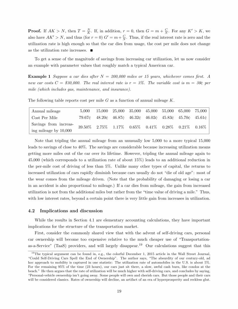
Example 1 Suppose a car dies after N = 200,000 miles or 15 years, whichever comes first. A

new car costs C = $30,000. The real interest rate is r = 3%. The variable cost is m = 30¢ per

mile (which includes gas, maintenance, and insurance).

The following table reports cost per mile G as a function of annual mileage K.

Annual mileage 5,000 15,000 25,000 35,000 45,000 55,000 65,000 75,000

Cost Per Mile 79.67¢ 48.20¢ 46.87¢ 46.32¢ 46.02¢ 45.83¢ 45.70¢ 45.61¢

Savings from increas-

ing mileage by 10,00039.50% 2.75% 1.17% 0.65% 0.41% 0.28% 0.21% 0.16%

Note that tripling the annual mileage from an unusually low 5,000 to a more typical 15,000

leads to savings of close to 40%. The savings are considerable because increasing utilization means

getting more miles out of the car over its lifetime. However, tripling the annual mileage again to

45,000 (which corresponds to a utilization rate of about 15%) leads to an additional reduction in

the per-mile cost of driving of less than 5%. Unlike many other types of capital, the returns to

increased utilization of cars rapidly diminish because cars usually do not “die of old age”: most of

the wear comes from the mileage driven. (Note that the probability of damaging or losing a car

in an accident is also proportional to mileage.) If a car dies from mileage, the gain from increased

utilization is not from the additional miles but rather from the “time value of driving a mile.” Thus,

with low interest rates, beyond a certain point there is very little gain from increases in utilization.

4.2 Implications and discussion

While the results in Section 4.1 are elementary accounting calculations, they have important

implications for the structure of the transportation market.

First, consider the commonly shared view that with the advent of self-driving cars, personal

car ownership will become too expensive relative to the much cheaper use of “Transportation-

as-a-Service” (TaaS) providers, and will largely disappear.19 Our calculations suggest that this

19The typical argument can be found in, e.g., the colorful December 1, 2015 article in the Wall Street Journal,“Could Self-Driving Cars Spell the End of Ownership”. The author says, “The absurdity of our century-old, adhoc approach to mobility is captured in one statistic: The utilization rate of automobiles in the U.S. is about 5%.For the remaining 95% of the time (23 hours), our cars just sit there, a slow, awful cash burn, like condos at thebeach.” He then argues that the rate of utilization will be much higher with self-driving cars, and concludes by saying,“Personal-vehicle ownership isn’t going away. Some people will own and cherish cars. But those people and their carswill be considered classics. Rates of ownership will decline, an artifact of an era of hyperprosperity and reckless glut.

19

view may not materialize. Consider a typical consumer—someone who drives 15,000 miles a year

(corresponding to an approximately 5% utilization rate) and lives in an area where parking is free

and readily available. For this consumer, the efficiency gain from switching away from car ownership

to using a TaaS fleet with three times higher utilization rate is less than 5%. Such a consumer may

easily choose to forgo this modest cost saving in favor of various benefits of personal car ownership,

such as, e.g., having a tennis racket or golf clubs in the trunk. Of course, for other consumers (e.g.,

those who live in areas where parking is very costly20 or those who drive very little), it would make

sense to use TaaS. Our framework in Section 3 naturally incorporates both models and allows them

to co-exist.

A closely related point is that beyond a fairly minimal utilization level, it is cheap for self-driving

cars to wait for a good nearby match with a rider or a group of riders, instead of repositioning the

car after a trip.21 This observation drives a key feature of our model in Section 3 that the cost of

a car trip only depends on the characteristics of that trip and not on the characteristics of other

trips in the system (if a car needed to be repositioned by a substantial distance from the end of

one trip to the beginning of the next one, or if waiting after the end of one trip until the beginning

of the next one was expensive, then the costs of trips would not be “separable”).

Proposition 1 implies that car-sharing platforms cannot deliver significant reductions in the

cost per mile relative to a typical personal car.22 For the relevant parameter range, the returns

to increased utilization are modest. This is in contrast to the airline industry, in which increasing

utilization is a high priority. The reason for this difference is that at 20,000 miles a year (which

corresponds to less than a 7% utilization rate), cars die after about 10 years, while airplanes can last

for decades at much higher utilization rates. If car manufacturers find a way to build cars that can

last for 20 years at double-digit utilization rates, just like planes do, then increasing utilization will

become a priority for TaaS fleet operators. Since self-driving cars can be utilized more intensively

than regular cars, automakers will have a stronger incentive than before to build more durable

cars. If and when cars become significantly more durable than they currently are, the economic

Twenty-five years from now, the only people still owning cars will be hobbyists, hot-rodders and flat-earth dissenters.Everyone else will be happy to share.”

Similarly, in a Bloomberg Television interview in November 2017, Jeff Holden, the chief product officer at Uber,said: “Our view is that individual car ownership is something that will go away because it is very inefficient. Individualowners use a car only 4 percent of the time, while with ride sharing a vehicle can be on the road 80 to 90 percent ofthe time. When you get to those kinds of utilizations what you see happen is prices go way down. So why would youown your own car? It’s just a hobby at that point. It just doesn’t make sense.”

20Calculations similar to those in Section 4.1 show that in areas where parking is very costly, the economic benefitof shared mobility (aside from that from carpooling, discussed below) is likely to come primarily from saving on thecost of parking rather than from getting more value out of the car.

21In most metropolitan areas, traffic flows are not perfectly balanced: e.g., in the mornings more cars are comingfrom suburbs to the downtown than in the opposite direction, and vice versa in the evenings. It is possible toincrease the utilization rate at the cost of having cars drive empty miles to get to high-demand areas. In light ofour calculations, even if it were possible to triple the utilization rate at the cost of increasing the number of “empty”miles by 5% of the total number of miles driven, such a trade-off would not be economically valuable.

22Indeed, in order to cover the overhead of operating the platform, car-sharing fleets such as Zipcar, Getaround,and Car2Go charge a significant premium relative to the cost per mile of a personal car. These car-sharing platformscreate economic value not because of more intensive use of a car, but because of the more intensive use of the parkingspot that the car occupies. For this reason, car-sharing platforms appear to succeed in areas where parking is scarce.

20

gain from increasing utilization may become significant, and so the economics and structure of the

transportation industry would also change.

There is another possible reason why car utilization may be more important than our example

suggests. We assumed that over the relevant time horizon, the cost of cars in real dollars remains

constant. Outside of the steady state, during times when the cost of making a car is expected

to decline, the cost decline can be incorporated into the model by increasing the interest rate

parameter by the expected annual cost reduction of self-driving cars. During the times when the

real price of new cars is expected to decline rapidly, increasing utilization may lead to significant

cost savings.

We conclude this section by highlighting the distinction between two ways of thinking about

“increasing car utilization.” One way is increasing the percentage of time the car is being used—

and that is the usual interpretation, and the one we considered in this section. The other way,

which we emphasize in Sections 2 and 3, is increasing the number of car seats that are utilized at

the times when the car is driving. As we have seen, doubling (or even tripling) the number of miles

a typical car is driven in a year reduces the cost per mile by less than 5%. In contrast, doubling

the average number of riders in the car reduces the cost per passenger by 50%. Thus, the potential

economic benefits of carpooling (higher seat utilization) are an order of magnitude greater than the

economic benefits of increasing the fraction of time each car is being used—even before we count

the positive externalities that carpoolers impose on other drivers by reducing traffic.

5 Concluding Remarks

We conclude with several remarks on our framework and results and their potential extensions

and generalizations.

One simplifying assumption in our model is that as long as the number of cars on a road segment

is below the segment’s capacity, the speed of the flow does not depend on the number of cars. In

other words, as long as the number of cars trying to go on a road segment is at its capacity or

below, there is no additional benefit to anyone from trying to reduce that number further (by further

raising the tolls, or by other means). As we discussed in Section 3.1, this approximation is very

accurate for highways: the maximum throughput is achieved at speeds close to the speed limit. For

cities, the relationship between the number of cars and traffic speed is more gradual. However, as in

the case of highways, the key consideration for efficient traffic management is to keep the demand

for travel below the level of hypercongestion, where both the speed of traffic and overall throughput

drop. This is the approach that our framework naturally incorporates. This approach, while only

an approximation of full social welfare maximization, has an important advantage that it can be

implemented based purely on data on traffic flows, without having to estimate or make judgments

about riders’ preferences. And implementing this approach would already be a major improvement

over the status quo. So we view this approach of focusing on the optimization of the overall flow of

traffic (as opposed to incorporating much more intricate utility trade-offs between speed and flow)

21

as the right first step for systemwide toll systems.23 Having said that, we should point out that our

framework also easily allows the regulator to implement more flexible traffic management policies.

While a traffic regulator cannot artificially increase the capacity qs of segment s, he can of course

artificially decrease it to any lower level q′s < qs. And our framework allows the same street to have

different capacities at different times of day. So if a regulator believes that at certain times and on

certain roads, it would be optimal to have traffic flows that are lower than those roads’ physical

capacities, our framework is flexible enough to accommodate this objective.

Another simplifying assumption made in our paper is that matches among carpooling partners

can be made frictionlessly. In other words, we implicitly assume that riders have access to a platform

that makes it easy to organize carpools. How such platforms will operate and compete is an open

question for future research.

Next, our model allows for time-varying demand for transportation, and accommodates time-

sensitive tolls. However, it assumes that demand fluctuations are known. A natural question is

how the model would change in a world with uncertainty, with unpredictable fluctuations in trans-

portation demand or road capacity. While the analysis of this question is beyond the scope of this

paper, we note that in many locations, traffic is quite predictable, occurring with regular patterns

(e.g., morning and evening commute times on weekdays). Thus, even if we restrict attention to

deterministic (but time-sensitive) tolls, and set the tolls in accordance with those regular patterns

to ensure that traffic flows freely a high fraction of the time, this deterministic policy may capture

much of the potential upside (relative to fully flexible stochastic tolls that adjust to demand and

supply fluctuations in real time).

Also, the presence of uncertainty raises the question of how much information should be disclosed

to commuters. Das et al. (2017) consider a model of congestion with solo drivers and no tolls, and

show that under uncertainty, suppressing some information may improve overall social welfare and

mitigate congestion. We leave to future research the analysis of the interplay between agents’

information sets, tolls, and carpooling in the presence of uncertainty.

We would like to conclude with a word of caution. Our paper proposes a “market solution” to

the question of designing an efficient transportation system: road prices are set by the regulator

at the market-clearing level, and a free coalition-formation market allows any groups of carpooling

partners to form. However, it is important to keep in mind that not all “market solutions” are

created equal: not every market solution would achieve an efficient outcome, or even get close to

it. For instance, privatizing roads and then letting road operators set prices freely would not work:

the revenue-maximizing profile of tolls may be very different from the efficiency-maximizing one.

Our approach proposes a market-based solution that does achieve a socially efficient outcome.

23In addition to being technically easier to implement, this approach is also more straightforward to communicateto the public, and may thus be more politically feasible.

22

References

Aumann, R. J. (1964). Markets with a continuum of traders. Econometrica 32 (1/2), 39–50.

Aumann, R. J. (1966). Existence of competitive equilibria in markets with a continuum of traders.

Econometrica 34 (1), 1–17.

Azevedo, E. M. and J. W. Hatfield (2015). Existence of equilibrium in large matching markets with

complementarities. Working Paper .

Azevedo, E. M., E. G. Weyl, and A. White (2013). Walrasian equilibrium in large, quasilinear

markets. Theoretical Economics 8 (2), 281–290.

Bator, F. M. (1961). On convexity, efficiency, and markets. Journal of Political Economy 69 (5),

480–483.

Das, S., E. Kamenica, and R. Mirka (2017). Reducing congestion through information design. In

Proceedings of the 55th Allerton Conference on Communication, Control, and Computing, pp.

1279–1284.

Farrell, M. J. (1959). The convexity assumption in the theory of competitive markets. Journal of

Political Economy 67 (4), 377–391.

Hall, F. L. (1996). Traffic stream characteristics. Traffic Flow Theory. US Federal Highway Ad-

ministration.

Hall, J. D. (2017). Pareto improvements from Lexus lanes. Journal of Public Economics, forth-

coming.

Koopmans, T. C. (1961). Convexity assumptions, allocative efficiency, and competitive equilibrium.

Journal of Political Economy 69 (5), 478–479.

Rothenberg, J. (1960). Non-convexity, aggregation, and Pareto optimality. Journal of Political

Economy 68 (5), 435–468.

Shapley, L. S. and M. Shubik (1966). Quasi-cores in a monetary economy with nonconvex prefer-

ences. Econometrica 34 (4), 805–827.

Small, K. A. and X. Chu (2003). Hypercongestion. Journal of Transport Economics and Pol-

icy 37 (3), 319–352.

Starr, R. M. (1969). Quasi-equilibria in markets with non-convex preferences. Econometrica 37 (1),

25–38.

Varaiya, P. (2005). What we’ve learned about highway congestion. Access Magazine 1 (27).

23

Vickrey, W. S. (1969). Congestion theory and transport investment. American Economic Re-

view 59 (2), 251–260.

Walters, A. A. (1961). The theory and measurement of private and social cost of highway congestion.

Econometrica 29 (4), 676–699.

24