Carpathian Journal of Electrical Engineering

No

rth

Un

ivers

ity o

f B

aia

Mare

C

arp

ath

ian

Jo

urn

al o

f E

lectr

ical E

ng

ineeri

ng

V

olu

me 4

, N

um

ber

1, 2010

Volume 4, Number 1, 2010North University of Baia Mare

Faculty of Engineering

Electrical Engineering Department

Carpathian Journal ofElectrical Engineering

NORDTECH PUBLISHERISSN 1843 - 7583

NORTH UNIVERSITY of BAIA MARE

FACULTY of ENGINEERING ELECTRICAL ENGINEERING DEPARTMENT

RO-430083, Baia Mare, Maramureş county, dr. Victor Babeş street, no. 62A,

phone: +40 (0) 362-401256 fax: +40 (0) 262-276153

http://www.ubm.ro

Carpathian Journal of Electrical Engineering

Volume 4, Number 1, 2010

ISSN 1843 – 7583

http://cee.ubm.ro/cjee.html

CHIEF EDITOR

Liviu Emil PETREAN North University of Baia Mare, Romania

MANAGING EDITOR

Mircea HORGOŞ North University of Baia Mare, Romania

EDITORIAL SECRETARY

Liviu NEAMŢ North University of Baia Mare, Romania

SCIENTIFIC BOARD

Theodoros D. TSIBOUKIS Aristotle University of Thessaloniki, Greece

Florin BREABĂN University Artois, France

Luis Adriano DOMINGUES Brazilian Electrical Energy Research Center, Brazil

Andrei VLADIMIRESCU University of California at Berkeley, USA

Tom O’DWYER Analog Devices, Ireland

Ştefan MARINCA Analog Devices, Ireland

Adam TIHMER University of Miskolc, Hungary

Jozsef VASARHELYI University of Miskolc, Hungary

Clint COLE Washington State University, SUA

Gene APPERSON Digilent Inc. SUA

Jan TURAN Technical University of Kosice, Slovakia

Andrei MARINESCU Research and Testing Institute ICMET, Romania

Emil SIMION Technical University of Cluj-Napoca, Romania

Iuliu DELESEGA Politehnica University of Timişoara, Romania

Alexandru SIMION Gheorghe Asachi Technical University of Iasi, Romania

Liviu Emil PETREAN North University of Baia Mare, Romania

Dan Călin PETER North University of Baia Mare, Romania

Constantin OPREA North University of Baia Mare, Romania

Carpathian Journal of Electrical Engineering Volume 4, Number 1, 2010

5

CONTENTS

Ioan ŢILEA

HIGH FREQUENCY ELECTROMAGNETIC PROCESSES IN INDUCTION MOTORS

SUPPLIED FROM PWM INVERTERS ...................................................................................... 7

Cristinel COSTEA

ON DISTRIBUTED MODEL PREDICTIVE CONTROL FOR LOAD FREQUENCY

PROBLEM ................................................................................................................................ 13

Olivian CHIVER, Liviu NEAMT, Zoltan ERDEI, Eleonora POP

CONSIDERATIONS REGARDING ASYNCHRONOUS MOTOR ROTOR PARAMETERS

DETERMINATION BY FEM .................................................................................................... 21

Liviu NEAMŢ, Arthur DEZSI

SWITCHED RELUCTANCE MOTOR OPTIMAL GEOMETRY DESIGN .............................. 29

Zoltan ERDEI, Paul BORLAN and Olivian CHIVER

COMPARISON BETWEEN ANALOG AND DIGITAL FILTERS ............................................ 37

Dumitru Dan POP, Vasile Simion CRĂCIUN, Liviu Neamţ, Radu Tîrnovan, Teodor

VAIDA

AN ECONOMICAL AND TECHNICAL CASE STUDY FOR A SMALL HYDROPOWER

SYSTEM .................................................................................................................................... 43

INSTRUCTIONS FOR AUTHORS ........................................................................................... 51


6


7

HIGH FREQUENCY ELECTROMAGNETIC PROCESSES IN

INDUCTION MOTORS SUPPLIED FROM PWM INVERTERS

Ioan ŢILEA

North University of Baia Mare

Key words: electromagnetic interference, inverter, induction motor

Abstract: The paper presents the electromagnetic interference between induction motors and inverters when at

high frequency electromagnetic process appears in induction motors having a parallel resonant effect because of

parasitic capacitive coupling between windings and ground, using a numerical model in simulink and a high

frequency induction motor equivalent circuit model this effect is shown.

1. INTRODUCTION

In modern PWM variable frequency AC motor drive the switching frequency is very

high, up to 200 kHz. The high frequency components of the inverter output voltage involves

electromagnetic interference problems, such as resonant parallel effect, due to the stray

capacitance between windings and ground. The output voltage of the inverter is generated as a

pulse string; the resultant current is modified substantially by the motor inductance and

consists basically of a sine wave at the fundamental frequency [1].

When supplying AC motors with high switching frequency because of the resonant

effect the motor inductance is modify and the current no longer consists of a sin wave but

becomes more like the inverter output voltage thus the di/dt greatly increases.

In order to predict the conducted electromagnetic interference, high frequency

induction motor equivalent circuit will be used.

2. THE BASIC MODELS

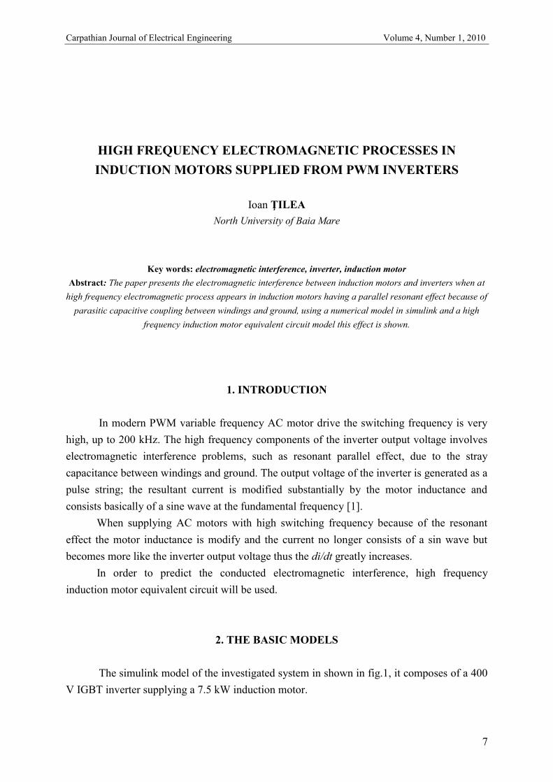
The simulink model of the investigated system in shown in fig.1, it composes of a 400

V IGBT inverter supplying a 7.5 kW induction motor.


8

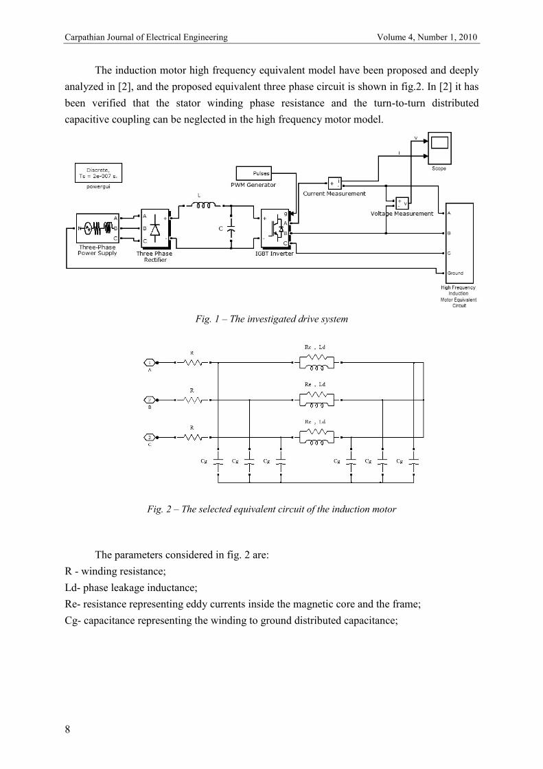
The induction motor high frequency equivalent model have been proposed and deeply

analyzed in [2], and the proposed equivalent three phase circuit is shown in fig.2. In [2] it has

been verified that the stator winding phase resistance and the turn-to-turn distributed

capacitive coupling can be neglected in the high frequency motor model.

Fig. 1 – The investigated drive system

Fig. 2 – The selected equivalent circuit of the induction motor

The parameters considered in fig. 2 are:

R - winding resistance;

Ld- phase leakage inductance;

Re- resistance representing eddy currents inside the magnetic core and the frame;

Cg- capacitance representing the winding to ground distributed capacitance;


9

3. SIMULATION RESULTS

The simulations were made in simulink using the models in fig.1 and fig. 2; the

fundamental frequency of the inverter has been keep at a constant 50 Hz only the switching

frequency is modify.

The values for the parameters considered in fig. 2 were obtained from [2], for a 7.5 kW

induction motor:

Cg= 0.953[nF];

Ld= 12.5[mH];

Re= 7.54[kΩ];

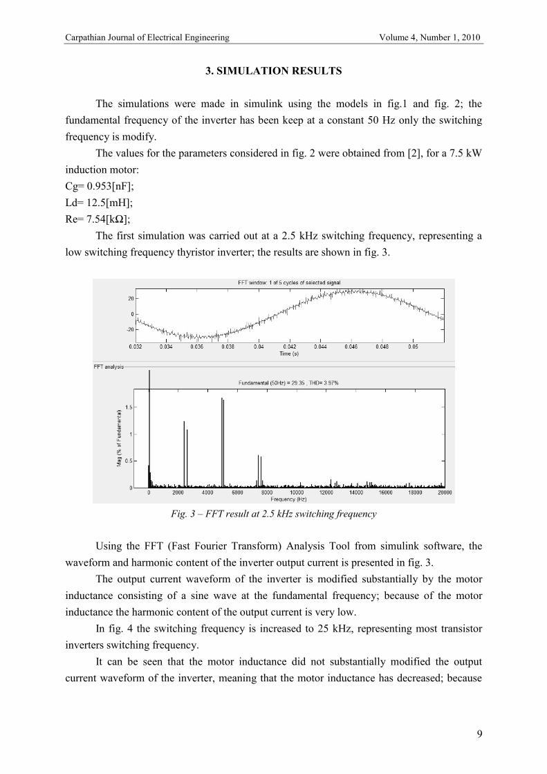
The first simulation was carried out at a 2.5 kHz switching frequency, representing a

low switching frequency thyristor inverter; the results are shown in fig. 3.

Fig. 3 – FFT result at 2.5 kHz switching frequency

Using the FFT (Fast Fourier Transform) Analysis Tool from simulink software, the

waveform and harmonic content of the inverter output current is presented in fig. 3.

The output current waveform of the inverter is modified substantially by the motor

inductance consisting of a sine wave at the fundamental frequency; because of the motor

inductance the harmonic content of the output current is very low.

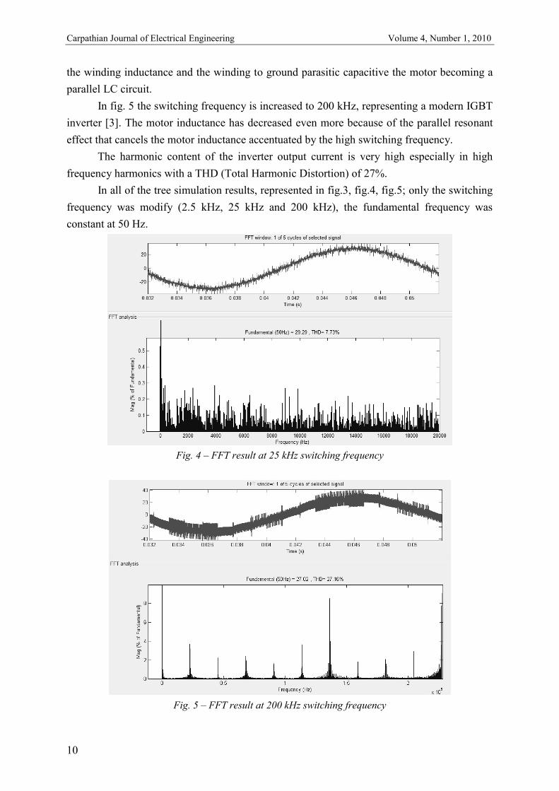
In fig. 4 the switching frequency is increased to 25 kHz, representing most transistor

inverters switching frequency.

It can be seen that the motor inductance did not substantially modified the output

current waveform of the inverter, meaning that the motor inductance has decreased; because


10

the winding inductance and the winding to ground parasitic capacitive the motor becoming a

parallel LC circuit.

In fig. 5 the switching frequency is increased to 200 kHz, representing a modern IGBT

inverter [3]. The motor inductance has decreased even more because of the parallel resonant

effect that cancels the motor inductance accentuated by the high switching frequency.

The harmonic content of the inverter output current is very high especially in high

frequency harmonics with a THD (Total Harmonic Distortion) of 27%.

In all of the tree simulation results, represented in fig.3, fig.4, fig.5; only the switching

frequency was modify (2.5 kHz, 25 kHz and 200 kHz), the fundamental frequency was

constant at 50 Hz.

Fig. 4 – FFT result at 25 kHz switching frequency

Fig. 5 – FFT result at 200 kHz switching frequency


11

4. CONCLUSION

At high switching frequencies the inverter power losses dramatically decreases so there

is an interest in making inverters that can work at high switching frequencies. Using a power

filter will minimize the effect of the high switching frequency but some application such as

vector control used in variable speed drives cannot work using output power filters.

High switching frequencies create electromagnetic interference problems between

inverter and motor in the form of resonant effects that cancels out the motor inductance,

increasing the di/dt output current of the inverter producing even more electromagnetic

interference along inverter-motor cable path.

REFERENCES

1. GAMBICA/REMA Technical Guide, Variable speed drives and motors, Technical Report No.2,

2002.

2. A. Boglietti, A. Cavagnino, M. Lazzari, Experimental high frequency parameter identification of

AC electrical motors, IEEE Xplore, 2005.

3. T. Friedli, S. D. Round, D. Hassler, J. W. Kolar, Design and performance of a 200 kHz All-SiC

JFET Current Source Converter, Industry Applications Society Annual Meeting, 2008.

4. J. Luszcz, K. Iwan, Conducted EMI propagation in inverter-fed AC motors, Electrical Power

quality and Utilisation, Magazine Vol. II, No.1, 2006.

5. S. Bartos, I. Dolezel, J. Necesany, J. Skramlik, V. Valouch, Theoretical and experimental

investigation of parasitic effects in induction motors drives supplied from semiconductor inverters,

Acta Electrotehnica et Informatica, Vol. 8, No. 4, 2008.


12


13

ON DISTRIBUTED MODEL PREDICTIVE CONTROL

FOR LOAD FREQUENCY PROBLEM

Cristinel COSTEA

North University from Baia Mare, Electric Department, [email protected]

Key words: Distributed Control, Load Frequency Control, Multi-Agent Systems

Abstract: The paper discribe a multi-agent application in power systems for the problem

of Load Frequency Control. The connections between subsystems are treated by each

controller agent as a set of disturbance signals. Each area maintain the tie-lines power

flow to specified values,based on communication between neighboring agents.

1. INTRODUCTION

One of the most implemented advanced control techniques in last decade in the

process industries [1] is Model Predictive Control (MPC), and its popularity is due to the

versatility in coping with constraints. The main concept of MPC is to use a model of the plant

to predict the future evolution of the system and is based on the idea of finite receding

horizon, emulating infinite horizon optimal control algorithms.

Using a model of the system to be controlled, at each sample period t an optimal

control problem is solved with the aid of constrained numerical optimization methods.

Following this, only the first part of the solution is implemented for the duration of the sample

period. Due to model uncertainty and disturbances, the actual output trajectory may deviate

from the predicted trajectory, thus a measurement of the actual output at the next sample

instant t + 1 is taken, and the optimal control problem is updated with the new measurement.

This process of measuring, solving a constrained optimization problem and implementing

only the first part of the optimal control sequence is repeated at future sample instants, and in

this way a feedback control law is produced. A thorough survey on the subject is [2].

From an algorithmic perspective, most MPC implementations result in the requirement

to solve, at each sample instant, a quadratic program (QP) :


14

(1)

This is a centralized approach that is considered impractical for the control problem of

large-scale systems (such as power networks), when the optimization problem is too big for

real time computation. The solution may be to decompose the problem into a set of smaller

subproblems and the overall system into appropriately subsystems with distinct MPC

controllers for each subsystem.

The new method of distributed MPC can be solved in a parallel manner if the

controllers are well coordinated; we intend to realize this by a particular communication

among the agents and not through a centralized supervisor. Thus, each subsystem problem

will be solved by an individual controller agent using local information and collaborating to

other agents to achieve global decisions.

Multi-agent systems (MAS) paradigm has matured during the last decade and effective

applications have been used; in MAS tasks are deploy by interacting entities (abstraction

objects named agents), capable of autonomous actions in its environment; agents cooperates

with each other, but each agent has incomplete information or capabilities for solving the

problem (has a limited viewpoint); there is no system global control, data are decentralized

and computation is asynchronous [3].

In industrial application agent technology can be use in process automation functions

where the tasks require cooperative distributed problem solving. Typical applications refer to

cooperative robots, sensor networks, traffic control, electronic markets. MAS can be

considered "self-organized systems" as they tend to find the best solution for their problems

without external intervention. Multi-agent technologies can be applied also, in a variety of

applications related to power system, such as disturbance diagnosis, restoration, secondary

voltage control or power system visualization [4].

2. MULTI-AGENT MODEL PREDICTIVE CONTROL

We will consider a network that is partitioned into subnetworks and each subsystem model

is represented as a discrete, linear time-invariant (LTI) model of the form (3)

(2)

where at time k for subsystem i, are local states, are the local

inputs, are the local known perturbation, are the local outputs and

are external influences due to interconnections between subsystems.

For each subsystem the controller will be implemented by a software agent; in each step

k the agent compute the next command solving an optimization problem (4) by

collaboration with other similar agents.


15

(3)

The expression of objective function from equation (4) can be expanded in order to

reformulate the MPC problem such as a quadratic programming (QP) problem for which

solvers are easy to find.

Just for simplicity will consider in next equations a prediction horizon N=3

(4)

and with following notations

, ,

, (5)

The weight matrix Qu , Qu from (3) is given by


16

(6)

and the objective function of agent i in step k can be written now as a QP problem:

(7)

The MPC problem in this form is echivalent to (4) for which standard and efficient

codes exist, many suppliers of MPC writing their own solvers [5]. The QP solver shipped

together with Matlab (quadprog) computes the answer with ten degrees of freedom or more in

well under a second, but generally are considered rather slow in terms of computational

speed; however Matlab provides a unified interface to other solvers.

The objective function (3) or (7) uses a quadratic cost function subject to the

constraints imposed on the manipulated variables as well as state or/and output variables,

expressing as a variable rate change or to keep the variable within certain bounds. According

to system equation (2), constraints can be formulated:

(8)

but it can be easly reformulated in term of equation (7).

The communication between agents can improve the predictions about the future

evolutions of interconnections variables. The observations in [6] suggest that information

exchange between neighboring agents can have a beneficial effect in stability, when it leads to

reduced prediction mismatch. As each system converges to its equilibrium, predictions on the

behavior of neighbors should get more and more accurate to satisfy the stability condition.

Each of the agents in the system can use MPC and through an iterative scheme

determine following actions, performing in parallel:

1) At sampling time instant k, agent i make a measurement of the current state of the

subsystem , send to and receive information from other neighboring agents.

2) Determine the best future behavior of local system according to a specified local

objective, solving an optimization problem over a certain horizon. During this

optimization there may be also communication with other agents.

3) Implement the first input of found actions until the next step.

4) Move horizon to the next sampling time. Move on to the next decision step.


17

3. MULTI-AREA POWER SYSTEM MODEL

The frequency is one of the main variables characterizing the power systems. The

purpose of load-frequency control (LFC) is to keep power generation equal to power

consumption under consumption disturbances, such that the frequency is maintained close to

a nominal frequency. LFC is becoming much more significant today due to deregulation of

power systems, and in last years a number of decentralized control strategies has been

developed for load-frequency control [7].

In a distributed manner, we consider more interconnected power subsystems where

each area must contribute to absorb any load change such that frequency does not deviate and

also, must maintain the tie-line power flow to its pre-specified value. If each considered area

is supervised by an controller agent, the agents have to obtain agreement with other agents on

power flowing over lines between subnetworks in order to be able to perform adequate local

frequency control.

Fig.1 – Diagram for the subsystem i of multi-area system

Models for electric power systems are generally nonlinear. However, for load

frequency control, the linearized model is generally used to design control schemes. Similar

to [7][8][9], Fig. 1 shows a block diagram for the ith subsystem of a multi-area power system.

The notations used in the dynamic model description of the ith area power subsystem

1,..,n are as follows:

∆fi incremental change in frequency (Hz)

∆ change in rotor angle

∆Pgi incremental change in generator output (p.u. MW)

∆Xvi incremental change in governor valve position (p.u. MW)

∆Pci incremental change in integral control

∆Pti incremental change in the tie line power (p.u. MW)


18

∆Pdi load disturbance (p.u. MW)

Tgi governor time constant (s)

Tti turbine time constant (s)

Tpi plant model time constant (s)

Kpi plant gain for ith area subsystem

Ri speed regulation due to governor action (Hz /p.u. MW)

The state variable equations from block diagram are derived as follows [8],[9]:

(9)

The differential equation for the power system:

(10)

(11)

The differential equation for the speed governor :

(12)

(13)

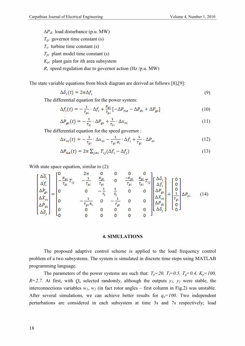
With state space equation, similar to (2):

(14)

4. SIMULATIONS

The proposed adaptive control scheme is applied to the load frequency control

problem of a two subsystems. The system is simulated in discrete time steps using MATLAB

programming language.

The parameters of the power systems are such that: Tp=20, Tt=0.5, Tg=0.4, Kp=100,

R=2.7. At first, with Qu selected randomly, although the outputs y1, y2 were stable, the

interconnections variables w1, w2 (in fact rotor angles – first column in Fig.2) was unstable.

After several simulations, we can achieve better results for qu=100. Two independent

perturbations are considered in each subsystem at time 3s and 7s respectively; load


19

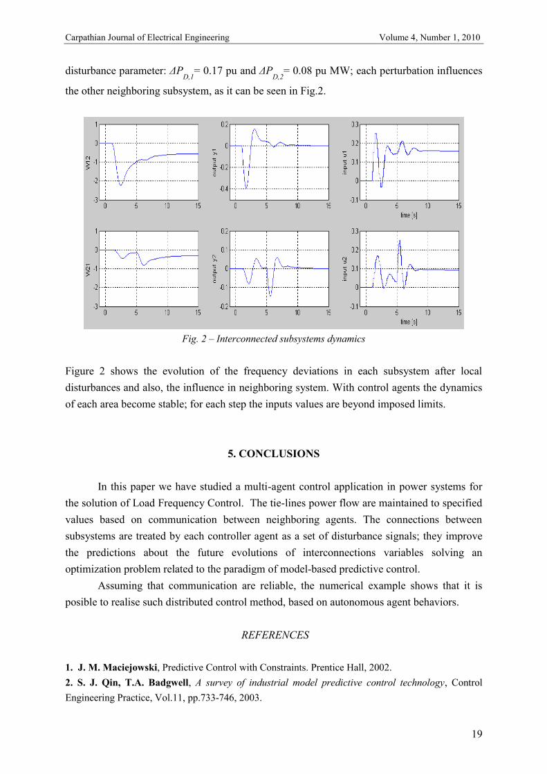
disturbance parameter: ΔPD,1

= 0.17 pu and ΔPD,2

= 0.08 pu MW; each perturbation influences

the other neighboring subsystem, as it can be seen in Fig.2.

Fig. 2 – Interconnected subsystems dynamics

Figure 2 shows the evolution of the frequency deviations in each subsystem after local

disturbances and also, the influence in neighboring system. With control agents the dynamics

of each area become stable; for each step the inputs values are beyond imposed limits.

5. CONCLUSIONS

In this paper we have studied a multi-agent control application in power systems for

the solution of Load Frequency Control. The tie-lines power flow are maintained to specified

values based on communication between neighboring agents. The connections between

subsystems are treated by each controller agent as a set of disturbance signals; they improve

the predictions about the future evolutions of interconnections variables solving an

optimization problem related to the paradigm of model-based predictive control.

Assuming that communication are reliable, the numerical example shows that it is

posible to realise such distributed control method, based on autonomous agent behaviors.

REFERENCES

1. J. M. Maciejowski, Predictive Control with Constraints. Prentice Hall, 2002.

2. S. J. Qin, T.A. Badgwell, A survey of industrial model predictive control technology, Control

Engineering Practice, Vol.11, pp.733-746, 2003.


20

3. K. Sycara,Multi-agent Systems,AI Magazine,The American Association for Artificial Intelligence,

10(2), pp. 79-93, 1998.

4. S. D. J. Mcarthur, E. M. Davidson, V. M. Catterson, A. L. Dimeas, N. D. Hatziargyriou, F.

Ponci, T. Funabashi, Multi-Agent Systems for Power Engineering Applications Part I: Concepts,

Approaches, and Technical Challenges, In Power Systems, IEEE Transactions on, Vol. 22, No. 4.

(2007), pp. 1743-1752.

5. J. A. Rossiter, Model-based Predictive Control - a Practical Approach, CRC Press, 2003.

6. T. Keviczky, F. Borrelli and G. J. Balas, Decentralized Receding Horizon Control for Large Scale

Dynamically Decoupled Systems, Automatica, December 2006, Vol. 42, No. 12, pp. 2105-2115.

7. H. Bevrani, Y. Mitani,K. Tsuji, Robust decentralised load-frequency control using an iterative

linear matrix inequalities algorithm, IEE Proceedings - Generation, Transmission and Distribution,

2004, 151(3):pp. 347-354.

8. M.T. Alrifai, M. Zribi, Decentralized Controllers for Power System Load Frequency Control,

ICGST International Journal on Automatic Control and System Engineering, 5(II), pp. 7-22, 2005.

9. M. Zribi, M. Al-Rashed, M. Alrifai, Adaptive decentralized load frequency control of multi-area

power systems, International Journal of Electrical Power & Energy Systems, 27(8), pp. 575-583, 2005.


21

CONSIDERATIONS REGARDING ASYNCHRONOUS MOTOR ROTOR

PARAMETERS DETERMINATION BY FEM

Olivian CHIVER, Liviu NEAMT, Zoltan ERDEI, Eleonora POP

North University of Baia Mare, email: [email protected], [email protected], [email protected],

[email protected].

Key words: asynchronous motor, rotor parameters, finite elements method.

Abstract: The paper presents some considerations about asynchronous motor rotor parameters determination,

using software based on finite elements method (FEM). For this, 2D magnetostatic and time harmonic analysis

will be realized, at different frequencies, in case of a three phase asynchronous motor.

1. INTRODUCTION

The asynchronous motor rotor parameters are determined experimentally by

two tests: no load test and short circuit test. Magnetization resistance and the sum between

stator leakage reactance and magnetization reactance are determined on the basis of

measurements realized in no load test. Based on measurements of short circuit test are

determined the short circuit resistance and reactance respectively. While the rotor resistance

at start moment can be determined from the short circuit resistance (the stator resistance can

be measured), the rotor leakage reactance can not be separated from the stator leakage

reactance. In order to determine the stator leakage reactance separately, the “removed rotor

method” [4] can be used.

2. PARAMETERS DETERMINATION BY FEM

Numerical methods development, especially FEM, makes possible the simulation of

any permanent or transient regime, therefore the previously presented methods can also be

simulated.


22

The ideal no load test assumes that the rotor speed is synchronous with the rotating

magnetic field generated by the stator winding (s=0), then no current is induced in rotor bars.

The rotor becomes exclusively a part of the nonlinear magnetic path for the stator magnetic

flux.

No load test numerical simulation by FEM can be realized by a 2D magnetostatic field

analysis, the goal being the magnetization reactance determination.

In case of an asynchronous motor with squirrel cage rotor (with high bars), double

layered stator winding with shortened pitch to 5/6, six notches per pole and phase, two poles

pair, the required numerical model for magnetostatic analysis is presented in figure 1.

Fig. 1. The numerical model

Since the rotating electrical machines are symmetrical, the numerical model

corresponds to a single pole, and the periodic boundary conditions are used.

The equivalent electrical circuit in case of no load regime is presented in fig. 2a. In

order to realize the simulation, current sources are used.

a) b) c)

Fig. 2. The equivalent electrical circuits


23

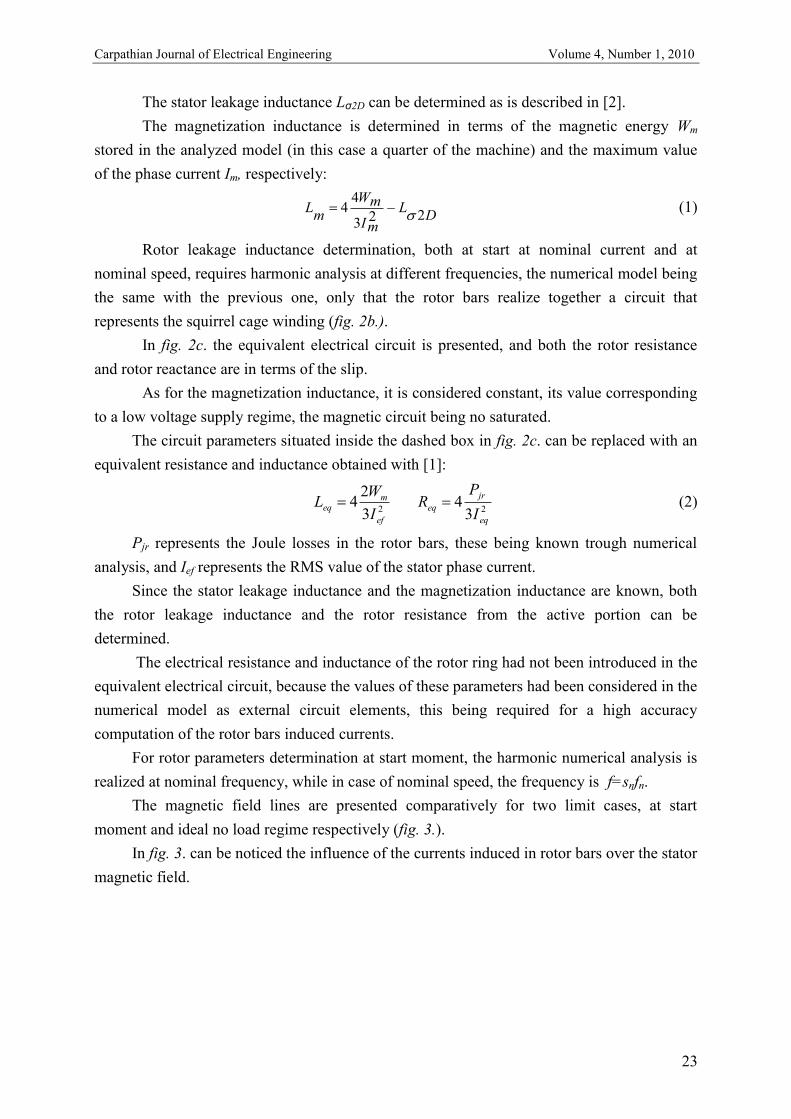
The stator leakage inductance Lσ2D can be determined as is described in [2].

The magnetization inductance is determined in terms of the magnetic energy Wm

stored in the analyzed model (in this case a quarter of the machine) and the maximum value

of the phase current Im, respectively:

DL

mI

mW

mL

223

44

(1)

Rotor leakage inductance determination, both at start at nominal current and at

nominal speed, requires harmonic analysis at different frequencies, the numerical model being

the same with the previous one, only that the rotor bars realize together a circuit that

represents the squirrel cage winding (fig. 2b.).

In fig. 2c. the equivalent electrical circuit is presented, and both the rotor resistance

and rotor reactance are in terms of the slip.

As for the magnetization inductance, it is considered constant, its value corresponding

to a low voltage supply regime, the magnetic circuit being no saturated.

The circuit parameters situated inside the dashed box in fig. 2c. can be replaced with an

equivalent resistance and inductance obtained with [1]:

23

24

ef

meq

I

WL

234

eq

jr

eqI

PR (2)

Pjr represents the Joule losses in the rotor bars, these being known trough numerical

analysis, and Ief represents the RMS value of the stator phase current.

Since the stator leakage inductance and the magnetization inductance are known, both

the rotor leakage inductance and the rotor resistance from the active portion can be

determined.

The electrical resistance and inductance of the rotor ring had not been introduced in the

equivalent electrical circuit, because the values of these parameters had been considered in the

numerical model as external circuit elements, this being required for a high accuracy

computation of the rotor bars induced currents.

For rotor parameters determination at start moment, the harmonic numerical analysis is

realized at nominal frequency, while in case of nominal speed, the frequency is f=snfn.

The magnetic field lines are presented comparatively for two limit cases, at start

moment and ideal no load regime respectively (fig. 3.).

In fig. 3. can be noticed the influence of the currents induced in rotor bars over the stator

magnetic field.


24

Fig. 3. Flux lines at start and at nominal speed

In case of asynchronous motors with high rotor bars or those with double squirrel cage,

the rotor parameters have different values at start moment and at nominal speed, because of

the non uniform current distribution in the rotor bars at high frequencies.

In fig. 4. the flux lines and current density in rotor bars are presented for two stator

current frequencies: 50Hz (the start moment) – left, and 2.5Hz (nominal speed) – right, in

case of an asynchronous motor with high bars.

Fig. 4. The current distribution in high rotor bars at start and at nominal speed

The variation of rotor leakage inductance and the rotor resistance in terms of current

frequency is presented in fig 5. in case of 55 kW asynchronous motor, with height of the rotor

bars 25 mm, and the height/width bar ratio 8.3.

Fig. 5. The rotor leakage reactance and rotor resistance in terms of frequency


25

For this motor, the equivalent rotor resistance decreases from 0.07 Ω at start moment to

0.04 Ω at 3% slip, decreasing 1.75 times, while the rotor leakage inductance increases from

0.49 mH at start moment to 1.04 mH at 3% slip, increasing 2.1 times.

In order to study the rotor parameters change, have been realized models representing

asynchronous motors with power in 5.5 – 1000 kW scale, and for each rotor the reduced

height of the bar has been computed with relation:

cr

rb

bh

20 (3)

Has been noted with h – high of the rotor bar, b – width of the rotor bar, bcr – width of

the notch, ρ – the electrical rotor bar resistivity, and ωr=2πfr.

The nominal slip values have been chosen in 0.05 – 1.6 scale, in terms of the motor

power, and the results regarding the value of the increasing resistance coefficient kr in terms

of the reduced height of the rotor bar ξ, for the analyzed models, are presented in fig. 6a.

The analytic curve that represents the variation of the increasing resistance coefficient kr

in terms of the reduced height of the rotor bar is presented comparatively.

A good concordance between analytically obtained and FEM results can be noticed.

a) b)

Fig. 6. The kr and kx coefficient in terms of reduced height of the rotor bar, ξ

The results obtained by presented method, regarding the variation of leakage inductance

from active portion of the rotor in terms of the reduced height of the rotor bar ξ, are showed in

fig 6b.

The comparison between the decreasing coefficient values, kx, obtained by FEM and

analytically, respectively, highlights the fact that, generally, for values of the reduced height

of the rotor bar ξ up to 1.66, the discrepancies are important.

The explanation consist in the following: leakage inductance of the rotor in nominal

regime determined according to the presented method is higher than the leakage inductance

corresponding to the start. This high value is due to the higher value of the magnetic energy

stored in the model analyzed at low frequency (at nominal regime) than the magnetic energy

stored in the model analyzed at nominal frequency (at start regime). Considering that this


26

increase of the magnetic energy is only due to the leakage inductance could explain the high

value of leakage inductance at nominal regime.

The detailed analysis of the models regarding the magnetic energy stored in different

parts of the machine however highlights that the most important increases are in the magnetic

circuit and in the air-gap.

Thus, if at start moment the magnetic energy stored in the magnetic circuit is

insignificant in comparison with the total energy, at nominal regime, this energy increases 20-

30 times, up to 10%. At start moment, the magnetic energy stored in the air-gap represents

about 30% from the total magnetic energy, and at nominal speed this energy comes up to

50%.

Based on these observations, for rotor slots leakage inductance determination, only the

magnetic energy stored in the rotor slots has been taken into consideration, the relation of

dependence being presented in (2).

In order to established the kx coefficient, it has been taken into consideration that only

leakage inductance corresponding to the rotor bar portion is affected by nonuniform

distribution of the current.

In figure 7., kx coefficient values obtained by FEM, based on magnetic energy stored in

rotor slots, are presented in terms of the reduced height of the rotor bar ξ.

Fig.7. The kx coefficient in terms of reduced height of the rotor bar, ξ, obtained by magnetic

energy stored in rotor slots

This time, a good concordance between analytically and FEM obtained results can be

noticed.

The values higher than one (up to 1.06), are due to the fact that in case of squirrel cage

rotor without high bars, at start moment the current distribution is uniform like at nominal

speed, fig. 8.


27

50 Hz 2.5 Hz

Fig. 8. The rotor bars current distribution in case of rotor without high bars

On the other hand, if at start moment the current distribution is uniform, more field lines

close by rotor slots (fig. 8.), and thus the value of the magnetic energy stored in rotor slots is

higher than that at nominal speed, although not all these lines represent the leakage field.

3. CONCLUZIONS

The computation of the rotor slots leakage inductance based on the first presented

method, leads to satisfactory results only in case of the machines with the reduced height of

the rotor bar generally higher than 1.66, in this case the rotor bars current distribution being

nonuniform.

The computation of the rotor leakage inductance and of kx coefficient based on the

magnetic energy stored in the rotor slots highlights a good concordance between analytically

and FEM results.

Thus can be noticed that the rotor leakage inductance determination from magnetic energy

stored in rotor slots has a satisfactory accuracy, the method could be applied in general case,

regardless of rotor bars shape.

REFERENCES

1. Bianchi N., „Electrical machine analysis using finite elements”, CRC Taylor & Francis Group,

2005;


28

2. Chiver O., Micu E., Barz C., „Stator winding leakage inductances determination using Finite

Elements Method”, 11th International Conference on Optimization of Electrical and Electronic

Equipment OPTIM'08, Braşov, România, May 22-24, 2008;

3 Cioc I., Nica C., „Proiectarea maşinilor electrice”, Ed.D.P., Bucuresti 1994;

4. Draganescu O. Gh., „Incercarile maşinilor electrice rotative”, Ed. Tehnică, Bucureşti 1987;

5. Fireţeanu V., “Modele numerice în studiul şi concepţia dispozitivelor electrotehnice”, Ed. Matrix

Rom, Bucureşti, 2004;

6. MagNet User‟s Guide;

7. www.infolytica.com/.../doccenter.

http://www.info-optim.ro/index.htm


http://www.infolytica.com/.../doccenter



29

SWITCHED RELUCTANCE MOTOR OPTIMAL GEOMETRY DESIGN

Liviu NEAMŢ, Arthur DEZSI

North University of Baia Mare, Romania, Eaton Electrical Group, Romania

[email protected]

Key words: SRM, Finite Element Method, Design

Abstract: This paper deals with the Switched Reluctance Motor (SRM) analysis using Finite Element Method

(FEM) for geometrical optimization in terms of volume ratio of torque on the rotor, the so-called specific torque.

The optimization parameter is the pair: stator and rotor pole angles, which forms a crucial part of the design

process.

1. INTRODUCTION

In the world market for electrical drives applications some domains, such as electric

traction motor, pumps and compressors at high speeds, robots and numerically controlled

machine tools, aeronautics and space technical, computer peripherals, etc., became clearly

dominated by the stepper motor - electronic converter assembly, known as SRM.

These led, unsurprisingly, to a huge interest from researchers, in obtaining a more

efficient motor and electronic converter and in development of design methods less

influenced by simplified assumptions with a high generality.

2. SRM PRELIMINARY DESIGN

SRM design should be initiated with a first step, so-called pre sizing, which provides

an initial set of geometric data.

Obtaining the diameter and length of stepper motor is considered in several works [1],

[2], [3] stems from the recommendations, in accordance with ISO, of the International

Electrotechnical Commission (IEC), by assimilation with asynchronous machine. The


30

preliminary selection of frame size goes automatically at the outer diameter of the stator. The

outer diameter of the stator is fixed in millimeters:

2)3( sizeframeDe , (1)

The rotor diameter is initially considered as the frame size, the feed-backs from design

procedure leading to required changes.

Once established these key dimensions it‟ll proceed to calculate the stator, βS and the

rotor, βR, pole arcs both expressed in radians, which is recommended to satisfy the following

relationships [2], [3], providing a maximum torque without engine to remain locked or to lose

steps:

RS , (2)

pS , (3)

R

RSZ

2 , (4)

The three relations describe a triangle so the SRM will function optimally only if the

stator and rotor pole angles will be found in this triangle. Fig.1. shows feasible triangle for a

8/6 machine. The region below OE represents condition 1, the region above GH represents

condition 2 and the region below DF represents condition 3. For example, if βS= 200 then

200< βR< 40

0.

Identification of optimal values for arcs involves calculating the maximum torque for

different combinations, as long as relations (2) - (4) only set some restrictions. Since

determining the maximum torque is subject to there overall package size of the resulting

motor, this step is one that sends to the initial phase of design for each new tested value of the

arc.

Fig. 1 - Feasible triangle for a 8/6 machine


31

Determination of machine torque can be done analytically from a number of

simplifying assumptions and magnetic equivalent circuit models.

FEM remains the best analysis tool. The easy way to accomplish the non linearity and

the complicated structure of the materials, great accuracy of the simulation, reduced costs,

speed of analysis permit to take into account a lot of models and choose the best fitting of a

desired imputed condition.

Will be considered a SRM prototype 8/6 which has the following characteristics:

Power output: 3728 [W]kwP

Speed: 1500 [ / min]N rot

Peak current: 13 [A]pi

Input AC voltage 480 [V]acV

The torque to be developed by the machine is:

3728=23.7459 [ ]

15002 2

60 60

kwPT N mN

, (5)

The machine will be designed with an IEC frame size of 100. The outer diameter of

the stator is fixed as follows:

0 3 2 100 3 2 194 [mm]D gabarit (6)

The maximum stack length for frame 100 is restricted to 200 mm: 200 [mm]L

For a machine of this frame size, a practical air-gap length can be assumed to be:

0.5 [mm]

The bore diameter D equal to the frame size is selected: D=100 [mm].

The remaining sizes are determined based on relatively simple relations and are not

elements of variability within the meaning of optimization in this paper.

So the only undetermined sizes are stator and rotor pole arcs. Using Fig.1, and

considering only the integer values of the angles resulted from triangle ABC, a total of 496

possible combinations become valid. Removing the combinations when s r and all

combinations over 5r s , because it follows a very high torque oscillation it remain to

be analyzed 80 possible combinations of rotor polar arc and polar arc stator, Fig. 2.


32

Fig. 2 - Combinations analyzed

3. SRM OPTIMIZATION

All 80 combinations of stator and rotor arc are carried out by FEM analysis using

Infolytica Magnet V 7 [5].

Fig. 3 – Optimized SRM

For example the geometry, final mesh and the magnetic field spectrum are presented

for two combinations:


33

Fig. 4 – SRM with βs = 150, βr=16

0. Resulted maximum torque of 22.37719369403 [Nm].

Fig. 5 – SRM with βs = 22

0, βr=23

0. Resulted maximum torque of 22.96590710053 [Nm].

Below are presented, in graphical form, the values of maximum torque for the 80

analyzed combinations of arcs stator – rotor:

Fig.6. Maximum SRM torque


34

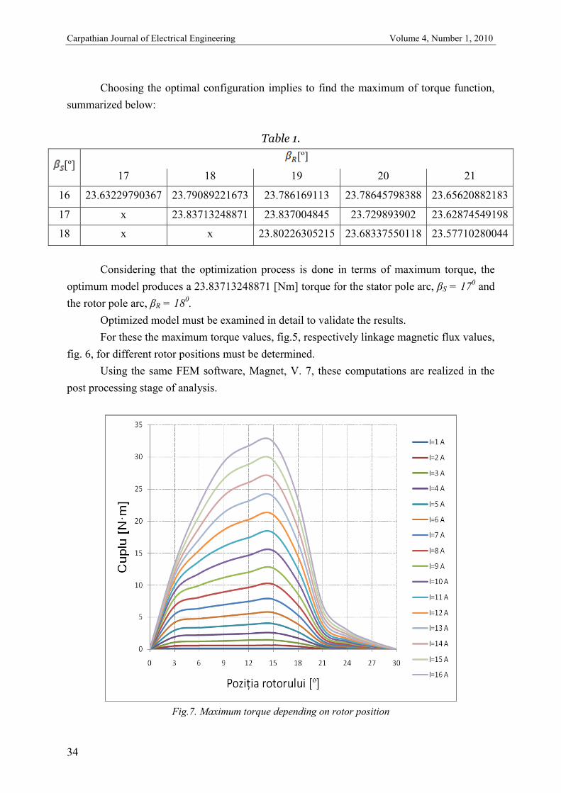
Choosing the optimal configuration implies to find the maximum of torque function,

summarized below:

Table 1.

[º] [º]

17 18 19 20 21

16 23.63229790367 23.79089221673 23.786169113 23.78645798388 23.65620882183

17 x 23.83713248871 23.837004845 23.729893902 23.62874549198

18 x x 23.80226305215 23.68337550118 23.57710280044

Considering that the optimization process is done in terms of maximum torque, the

optimum model produces a 23.83713248871 [Nm] torque for the stator pole arc, βS = 170 and

the rotor pole arc, βR = 180.

Optimized model must be examined in detail to validate the results.

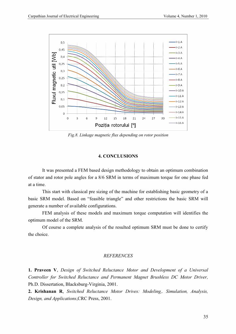
For these the maximum torque values, fig.5, respectively linkage magnetic flux values,

fig. 6, for different rotor positions must be determined.

Using the same FEM software, Magnet, V. 7, these computations are realized in the

post processing stage of analysis.

Fig.7. Maximum torque depending on rotor position


35

Fig.8. Linkage magnetic flux depending on rotor position

4. CONCLUSIONS

It was presented a FEM based design methodology to obtain an optimum combination

of stator and rotor pole angles for a 8/6 SRM in terms of maximum torque for one phase fed

at a time.

This start with classical pre sizing of the machine for establishing basic geometry of a

basic SRM model. Based on “feasible triangle” and other restrictions the basic SRM will

generate a number of available configurations.

FEM analysis of these models and maximum torque computation will identifies the

optimum model of the SRM.

Of course a complete analysis of the resulted optimum SRM must be done to certify

the choice.

REFERENCES

1. Praveen V, Design of Switched Reluctance Motor and Development of a Universal

Controller for Switched Reluctance and Permanent Magnet Brushless DC Motor Driver,

Ph.D. Dissertation, Blacksburg-Virginia, 2001.

2. Krishanan R, Switched Reluctance Motor Drives: Modeling,. Simulation, Analysis,

Design, and Applications,CRC Press, 2001.


36

3. Miller, TJE, Switched Reluctance Motors and their Control, Magna Physics Publishing

and Clarendon Press, Oxford, 1993.

4. Torkaman, H. Afjei E, Comprehensive study of 2-D and 3-D finite element analysis of a switched

reluctance motor. J. Applied Sci., 8: 2758-2763, 2008.

5. Magnet CAD Package, User Manual. Infolytica Corporation Ltd., Montreal, Canada, 2007.

6. Faiz J, Ganji B, De Doncker R. W, Fiedler J.O, Electromagnetic Modeling of Switched

ReluctanceMotor Using Finite Element Method, IEEE Industrial Electronics, IECON 2006.

7. Lee J. W, Kim H. K, Kwon B. I, Kim B. T, New Rotor Shape Design for Minimum Torque Ripple

of SRM Using FEM, IEEE Transactions on Magnetics, Vol. 40, No. 2, March 2004.


37

COMPARISON BETWEEN ANALOG AND DIGITAL FILTERS

Zoltan ERDEI*, Paul BORLAN** and Olivian CHIVER*

* North University of Baia Mare, Romania

[email protected]

Key words: analog filters, digital filters, signal proccesing

Abstract: Digital signal processing(DSP) is one of the most powerful technologies and will model science and

engineering in the 21st century. Revolutionary changes have already been made in different areas of research

such as communications, medical imaging, radar and sonar technology, high fidelity audio signal reproducing

etc. Each of these fields developed a different signal processing technology with its own algorithms, mathematics

and technology, Digital filters are used in two general directions: to separate mixed signals and to restore

signals that were compromised in different modes. The objective of this paper is to compare some basic digital

filters versus analog filters such as low-pass, high-pass, band-pass filters. Scientists and engineers comprehend

that, in comparison with analog filters, digital filters can process the same signal in real-time with broader

flexibility. This understanding is considered important to instill incentive for engineers to become interested in

the field of DSP. The analysis of the results will be made using dedicated libraries in MATLAB and Simulink

software, such as the Signal Processing Toolbox.

1. INTRODUCTION

Analog filters are a first layer block in signal processing, often used in electronics.

Passive filters have been the base of communications since the 1920‟s and are of considerable

importance for frequencies situated between 100 and 500 kHz. Hundreds, if not thousands of

types of passive filters have been developed in order to satisfy the needs of different

applications. However most filters can be described by few common charactheristics. First

of them is the frequency domain of their bandpass. The bandpass of a filter is frequency

domain over which an input signal will pass. Signals of frequencies that are not in the

bandpass will be attenuated.

2. LOWPASS FILTER

Lowpass filters allow low frequency signals to pass, while they block high frequency


38

signals. The concept of lowpass filter exists in various forms, including electronic circuits,

digital algorithms used to process data sets, acoustic barriers, image processing etc. Low-pass

filters play the same role in signal processing that moving averages do in some other fields,

such as finance; both tools provide a smoother form of a signal which removes the short-term

oscillations, leaving only the long-term trend. In equation (1) you can see the break

frequency, also called the turnover frequency or cutoff frequency (in Hz).

(1)

where R is the resistor, with a value in ohms, and C is the capacitor, with a value in Farads.

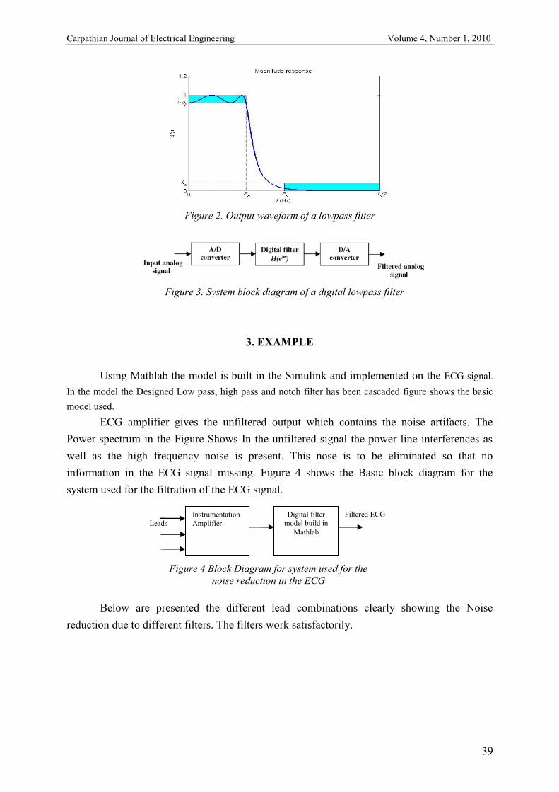
In figure 1 you can see the analog realization of a lowpass filter and in figure 2 you

can see the output waveform of a lowpass filter.

Same filter response can be obtained using a digital filter as shown by the system

block diagram in figure 3. The analog signal x(t) is converted into a discrete-time signal x(n),

which is processed by the digital filter, to yield a discrete-time output y(n). Finally, the

discrete output y(n) is converted into an analog form y(t). The cutoff frequency of digital

filter response H(ejώ

) is related to the analog cutoff frequency through the important analog-

digital frequency relation

ώ=ΏT (2)

where T(s) is the sampling interval of discrete-time system.

Hence, the unit of analog frequency, Ώ, is radians/s and while the unit of digital

frequency, ώ, is radians.

The digital filter can be realized using a Digital Signal Processor (DSP). The DSP can

be programmed to act as any kind of filter. This is one of the main advantages of digital

systems.

In digital processing the signal is represented by a signal of numbers that are stored

and then processed.

Figure 1. Analog realization of lowpass filter


39

Figure 2. Output waveform of a lowpass filter

Figure 3. System block diagram of a digital lowpass filter

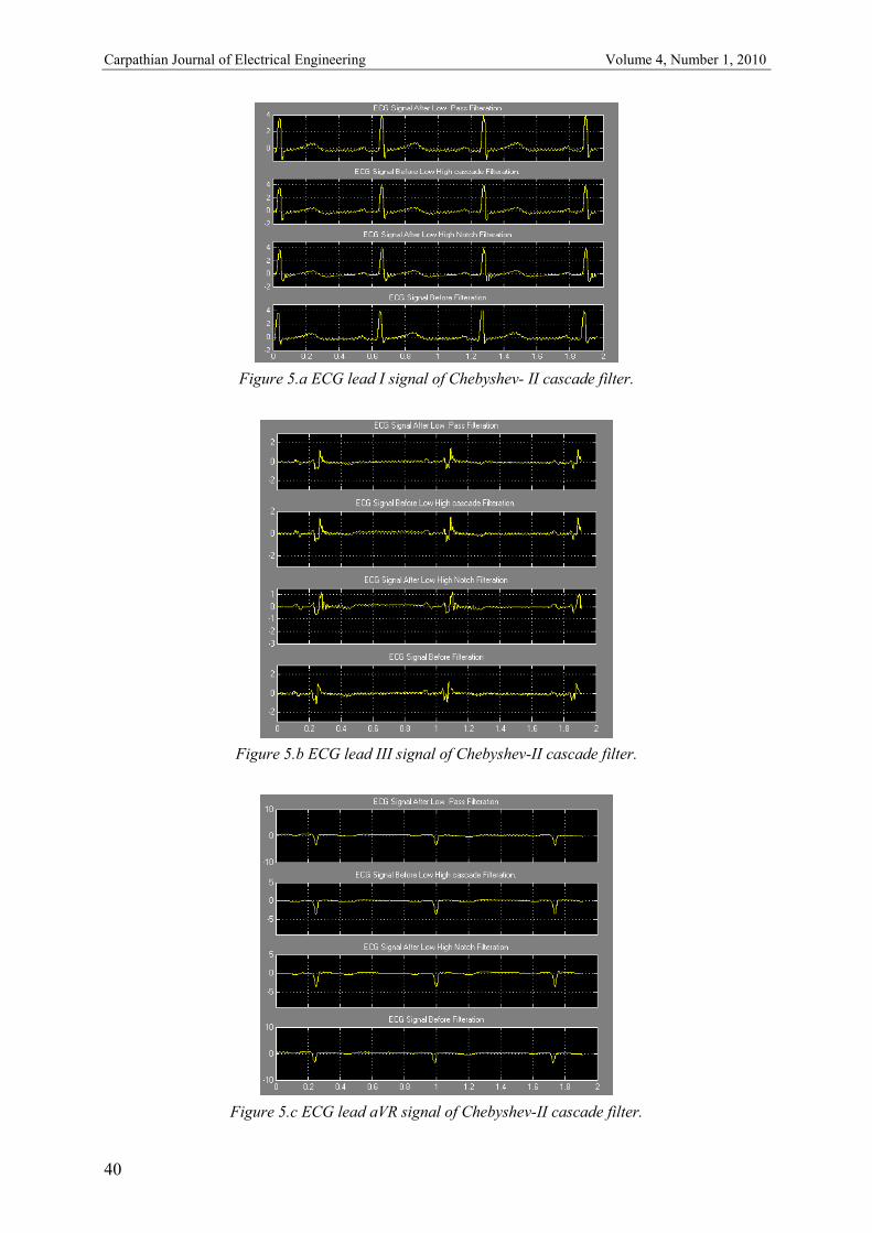
3. EXAMPLE

Using Mathlab the model is built in the Simulink and implemented on the ECG signal.

In the model the Designed Low pass, high pass and notch filter has been cascaded figure shows the basic

model used.

ECG amplifier gives the unfiltered output which contains the noise artifacts. The

Power spectrum in the Figure Shows In the unfiltered signal the power line interferences as

well as the high frequency noise is present. This nose is to be eliminated so that no

information in the ECG signal missing. Figure 4 shows the Basic block diagram for the

system used for the filtration of the ECG signal.

Below are presented the different lead combinations clearly showing the Noise

reduction due to different filters. The filters work satisfactorily.

Instrumentation

Amplifier

Digital filter

model build in

Mathlab

Filtered ECG

Leads

Figure 4 Block Diagram for system used for the

noise reduction in the ECG


40

Figure 5.a ECG lead I signal of Chebyshev- II cascade filter.

Figure 5.b ECG lead III signal of Chebyshev-II cascade filter.

Figure 5.c ECG lead aVR signal of Chebyshev-II cascade filter.


41

Figure 6.a Frequency Spectrum for Chebyshev II Filter Before Filtration of the ECG Signal

Figure 6.b Frequency Spectrum for Chebyshev II Filter after Filtration of the ECG Signal.

4. CONCLUSIONS

With visualization of above results by appropriate design if the Digital Chebyshev

type II Filter the noise in the ECG signal can be effectively reduced.

Throughout our experiments we used MATLAB and SIMULINK in order to simulate

de filter and process the input signal.

Some of the key features that distinguish digital filters from analog filters are: digital

filters are programmable, implemented using software packages, can easily be changed or

updated without affecting their circuitry (hardware), can be designed, tested and implemented

on a general purpose computer, are independable of physical variables such as temperature,

tolerances of elements, noise, fluctuations or inteferences. Analog filters use elements that

are environment dependent, and any filter change is usually hard to implement and a complete

design is often required.

REFERENCES

1. Wai-Kai Chen, “Passive, active and digital filters”, Ed. CRC Press, 2006

2. Robert J. Shilling, Sandra L. Harris, “Fundamentals of digital signal processing using Matlab”,

Ed. Thomson, 2005

3. Steven W. Smith, “The scientist and engineer’s guide to digital signal processing”, 2nd

edition,

California Technical Publishing, 1999


42

4. MAHESH S. CHAVAN Application of the Chebyshev Type II Digital Filter For Noise Reduction

In ECG Signal Proceedings of the 5th WSEAS Int. Conf. on Signal Processing, Computational

Geometry & Artificial Vision, Malta, September 15-17, 2005 (pp1-8)

5. Scokolow M., Mcllory M.B. and Cheithen,M.D’ ClinicalCardiology‟; 5th ed (VALANGEMedical

Book, 1990).

6. P.K.Kulkarni,Vinod Kumar,“ Removal of power line interference and baseline wonder using real

time Digital filter”, Proceedings of international conference on computer application in electrical

engineering Recent advantages. Roorkee, India. September 1997, pp 20-25.

7. Huta, J.C. and Webster. J.G. 1973, “60 Hz Interferences Electrocardiography”, IEEE trans. BME

-20, pp 91-101.

8. Marques.De.Sa.J.P. “Digital FIR filtering for removel of baseline wonder,” Journal of Clinical

Engineering vol. pp. 235-240.

9. Yi-Sheng, Zhu,et al. “ P-wave detectionby an adaptive QRS-T cancellation technique”.1987


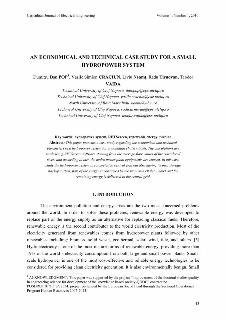
43

AN ECONOMICAL AND TECHNICAL CASE STUDY FOR A SMALL

HYDROPOWER SYSTEM

Dumitru Dan POP1, Vasile Simion CRĂCIUN, Liviu Neamţ, Radu Tîrnovan, Teodor

VAIDA

Technical University of Cluj Napoca, [email protected]


North University of Baia Mare [email protected]



Key words: hydropower system, RETScreen, renewable energy, turbine

Abstract: This paper presents a case study regarding the economical and technical

parameters of a hydropower system for a mountain chalet - hotel. The calculations are

made using RETScreen software starting from the average flow values of the considered

river, and according to this, the hydro power plant equipments are chosen. In this case

study the hydropower system is connected to central grid but also having its own storage

backup system, part of the energy is consumed by the mountain chalet – hotel and the

remaining energy is delivered to the central grid.

1. INTRODUCTION

The environment pollution and energy crisis are the two most concerned problems

around the world. In order to solve these problems, renewable energy was developed to

replace part of the energy supply as an alternative for replacing classical fuels. Therefore,

renewable energy is the second contributor to the world electricity production. Most of the

electricity generated from renewables comes from hydropower plants followed by other

renewables including: biomass, solid waste, geothermal, solar, wind, tide, and others. [5]

Hydroelectricity is one of the most mature forms of renewable energy, providing more than

19% of the world‟s electricity consumption from both large and small power plants. Small-

scale hydropower is one of the most cost-effective and reliable energy technologies to be

considered for providing clean electricity generation. It is also environmentally benign. Small

1 ACKNOWLEDGMENT: This paper was supported by the project "Improvement of the doctoral studies quality

in engineering science for development of the knowledge based society-QDOC” contract no.

POSDRU/107/1.5/S/78534, project co-funded by the European Social Fund through the Sectorial Operational

Program Human Resources 2007-2013.


44

hydro is in most cases “run-of-river”; in other words any dam or barrage is quite small,

usually just a weir, and little or no water is stored. Therefore run-of-river installations do not

have the same kinds of adverse effect on the local environment as large-scale hydro (they do

not have negative effects to the environment such as replacement of settlements, loss of

historical sites and agricultural fields, destruction of ecological life). [12]

Each hydro site is unique, since about 75% of the development cost is determined by

the location and site conditions. Only about 25% of the cost is relatively fixed, being the cost

of manufacturing the electromechanical equipment. The development of small hydro projects

typically takes from 2 to 5 years to complete, from conception to final commissioning. This

time is required to undertake studies and design work, to receive the necessary approvals and

to construct the project. Once constructed, small hydro plants require little maintenance over

their useful life, which can be well over 50 years. Normally, one part-time operator can easily

handle operation and routine maintenance of a small hydro plant, with periodic maintenance

of the larger components of a plant usually requiring help from outside contractors. [1]

Although there is no universally agreed definition for „„small hydro‟‟, the upper limit

varies between 2.5 and 25MVA and a maximum of 10MW is the most widely accepted value

worldwide. The terms mini- and micro-hydro are also used to refer to groupings of capacity

below the „„small‟‟ designation. Generally in industrial terms, mini- and micro-hydro

typically refer to schemes below 2MW and below 500kW, respectively. These are arbitrary

divisions and many of the principles involved apply to both smaller and larger schemes. [4]

Small hydropower systems allow achieving self-sufficiency by using the best as

possible the scarce natural resource that is the water, as a decentralized and low-cost of

energy production, since they are in the forefront of many developing countries. In Europe the

development of small hydroelectricity grows up since the seventy decade, essentially, caused

by the world energy crisis, and the concerns of negative environmental impacts associated to

the energy production. Hydropower is the most important energy source in what concerns no

carbon dioxide, sulphur dioxide, nitrous oxides or any other type of air emissions and no solid

or liquid wastes production. The introduction of innovative solutions coupled to renewable

energy technologies should contribute to a substantial global reduction in emission of CO2

and other gases, which are responsible for greenhouse effects. The hydroelectric power plant

utilizes a natural or artificial fall of a river and enhances the main advantages comparing with

other electricity sources, namely saving consumption of fossil, fuel, or firewood, being self-

sufficient without the need of imported components. [11]

Hydroelectricity is now recognized as key technologies in bringing renewable

electricity to rural populations in developing countries, many of whom do not have access to

electric power. [7] Typically, small hydro generation is located close to the end-user which

reduces or eliminates transmission losses and it gives independence from the world‟s fossil

fuel fluctuations. [6]


45

2. DESCRIPTION OF SMALL HYDROPOWER SYSTEM

A hydropower system has the following mechanical and electrical components: a

water turbine that converts the energy of flowing or falling water into mechanical energy that

drives a generator which generates electrical power, a control mechanism to provide stable

electrical power and electrical transmission lines to deliver the power to its destination. [2]

Hydropower systems use the energy in flowing water to produce electricity or

mechanical energy. Although there are several ways to harness the moving water to produce

energy, run-of-the-river systems, which do not require large storage reservoirs, are often used

for microhydro, and sometimes for small-scale hydro, projects. For run-of-the-river hydro

projects, a portion of a river‟s water is diverted to a channel, pipeline, or pressurized pipeline

(penstock) that delivers it to a waterwheel or turbine. The moving water rotates the wheel or

turbine, which spins a shaft. The motion of the shaft can be used for mechanical processes,

such as pumping water, or it can be used to power an alternator or generator to generate

electricity. This fact sheet will focus on how to develop a run-of-the-river project. [8] In fig. 1

is presented a functional scheme of a small hydropower

The amount of power available from a hydropower system is directly related to the

flow rate, head, the force of gravity and a efficiency factor. The theoretical power output (in

kW) can be calculated using the following equation:

egHQP (1)

where:

Q = usable flow rate (m3/s);

H = Gross head (m);

g = Gravitational constant (9.8 m/s2);

e = efficiency factor (0.5 to 0.7).

Fig. 1 - Small Hydro System Description

Head (m) Head (m)

Flow (m3/s)


46

There are two types of turbines, impulse and reaction. For each application the turbine

is chosen depending on the head and flow available. In table 1 we present different types of

water turbines. [2]

Table1. Transposing principle

Turbine runner High head

(more than 100 m)

Medium high

(20 to 100 m)

Low head

(5 to 10 m)

Ultra-low head

(less than 5 m)

Impulse Pelton

Turgo

Cross-flow

Turgo

Multi-Jet Pelton

Cross-flow

Multi-Jet Pelton

Water wheel

Reaction - Francis

Pump-as-turbine

Propeller

Kaplan

Propeller

Kaplan

The „capacity factor‟ is a ratio summarizing how hard a turbine is working, expressed

as follows:

yearhourskWcapacityinstalled

yearkWHyearpergeneratedenergyfactorcapacity

/8760)(

)/((%)

(2)[3]

Generators convert the mechanical (rotational) energy produced by the turbine to

electrical energy. There are two types of generators: synchronous and asynchronous.

Synchronous generators are standard in electrical power generation and are used in most

power plants. Asynchronous generators are more commonly known as induction generators.

Both of these generators are available in three-phase or single-phase systems. [2]

3. CASE STUDY AND RESULTS

The case study is for a mountain chalet - hotel with 30 rooms in a tourist area. The

need for electrical energy is all over the year because the area has ski slopes in winter and

rafting, climbing and other summer activities. The flow is from a real river but by economical

reasons we can‟t provide the name and the location of it. The analyze is made using

RETScreen software which is a decision support tool developed with the contribution of

numerous experts from Canadian government, industry, and academia. The software can be

used to evaluate the energy production and savings, costs, emission reductions, financial

viability and risk for various types of renewable energy.

The hydropower system is connected to central grid (20 kW) witch is located nearby.

We chose to have backup batteries so we use synchronous generators and an inverter. We

have made a list of consumers resulting the electrical power necessary for the building, the

installed power Pi=70 kW.


47

The water intake location was chosen at the limit with the protected area so that we

can obtain all the necessary approvals, the type of water intake is Tyrolean. The location

where the power house will be located belongs to the owner of the mountain chalet – hotel.

The distance between the intake and the power house is 2500 m resulting a head of 100 m.

The connection between intake and power house will be made with an PAFSIN GRP

adduction, with diameter D=600 mm and asperity e=0,03 mm. In calculating the diameter of

the adduction the maximum hydraulic losses was considered 6,6%.

Knowing the head (100 m) and the design flow (0,430 m3/s) we have chosen from

product database a single impulse turbine, Pelton model, manufactured by Voith Siemens.

(Fig. 2)

Fig. 2 – Inserted data and results from RETScreen

After inserting the flow values in the program according to the hydro data achieved from

Hydrological Institute (table 2), we obtained the following turbine efficiency curve (Fig. 3)

and flow duration and power curves (Fig. 4) for that specific river. The firm flow (0.44 m3/s)

was calculated by the software after inserting the hydrological data and residual flow (0,091

m3/s).

Table 2. Hydrological data and results for turbine efficiency and combine efficience


48

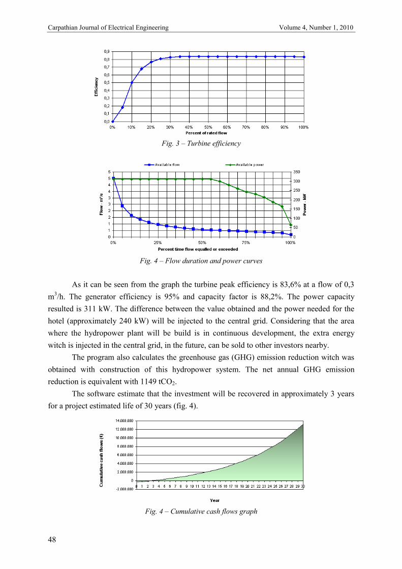
Fig. 3 – Turbine efficiency

Fig. 4 – Flow duration and power curves

As it can be seen from the graph the turbine peak efficiency is 83,6% at a flow of 0,3

m3/h. The generator efficiency is 95% and capacity factor is 88,2%. The power capacity

resulted is 311 kW. The difference between the value obtained and the power needed for the

hotel (approximately 240 kW) will be injected to the central grid. Considering that the area

where the hydropower plant will be build is in continuous development, the extra energy

witch is injected in the central grid, in the future, can be sold to other investors nearby.

The program also calculates the greenhouse gas (GHG) emission reduction witch was

obtained with construction of this hydropower system. The net annual GHG emission

reduction is equivalent with 1149 tCO2.

The software estimate that the investment will be recovered in approximately 3 years

for a project estimated life of 30 years (fig. 4).

Fig. 4 – Cumulative cash flows graph


49

4. CONCLUSIONS

We have chosen an optimal positioning of the intake and power plant to obtain a

maximum head. The Tyrolean intake is located on the main river, in the most concentrated

area in terms of affluent river s so we can take a higher flow, outside the protected area.

The optimal diameter for the adduction was chose for not having higher hydraulic

losses. By using the PAFSIN GRP material for adduction because it has smaller asperity, we

obtained a diameter of 600 mm, comparing with a steel adduction witch would be with 100

mm bigger.

The design flow was chosen smaller than the firm flow resulting a constant function of

turbine during the entire year, considering that the river flow is variable and it also ensures the

power needed for the mountain chalet – hotel. Even more, it provides profit by injecting the

remaining power into the central grid.

The turbine will operate at maximal parameters about 60% of the year according to the

graphics obtained through the RETScreen software.

Electricity production from hydropower has been, and still is today, the first renewable

source used to generate electricity. Nowadays hydropower electricity in the European Union

both large and small scale represents 13% of the total electricity generated, so reducing the

CO2 emissions by more than 67 million tons a year.

The most important advantages that hydropower systems have over wind, wave and

solar power are:

• a high efficiency (70 - 90%), by far the best of all energy technologies;

• a high capacity factor (typically >50%), compared with 10% for solar and 30% for wind;

• a high level of predictability, varying with annual rainfall patterns;

• slow rate of change; the output power varies only gradually from day to day (not from

minute to minute);

• a good correlation with demand i.e. output is maximum in winter;

• it is a long-lasting and robust technology; systems can readily be engineered to last for 50

years or more.

RETScreen is a very useful tool for verifying technical and economical aspects for a

hydropower system. Using this software we were able obtain information that this

hydropower system can provide the necessary power needed for the hotel and also an

estimated period for recover the initial investment.

REFERENCES

[1] Natural Resources Canada, Small hydro project analysis chapter, Canada 2004

[2] Natural Resources Canada, Micro-Hydropower systems, Canada, 2004

[3] The British Hydropower Association, A guide to UK mini-hydro developments, UK, 2005


50

[4] Y. Aslana, O. Arslanb, C. Yasara, A sensitivity analysis for the design of small-scale

hydropower plant: Kayabogazi case study, Renewable energy, volume 33, pp. 791-801, 2007

[5] R. Bakis, Electricity production opportunities from multipurpose dams (case study),

Renewable energy, volume 32, pp. 1723-1738, 2007

[6] K. V. Alexander, E. P. Giddens, Microhydro: Cost-effective, modular systems for low

heads, Renewable energy, volume 33, pp. 1379-1391, 2008

[7] A. A. Williams, R. Simpson, Pico hydro – Reducing technical risks for rural

electrification, Renewable energy, volume 34, pp. 1986-1991, 2009

[8] U.S.A. National Renewable Energy Laboratory, Small hydropower systems, USA, 2001

[9] G. Taljan, A.F. Gubina, Energy-based system well-being analysis for small systems with

intermittent renewable energy sources, Renewable energy, volume 34, pp. 2651-2661, 2009

[10] European Small Hydropower Association, Guide on how to develop a small

hydropower plant, 2004

[11] H. Ramos, B. A. de Almeida, Small hydropower schemes as an important renewable

energy source, International Conference Hidroenergia (99), Vienna, Austria, 1999

[12] http://www.retscreen.net/


51

INSTRUCTIONS FOR AUTHORS

Name SURNAME, Name Surname, ...

Affiliation, email of 1st author, Affiliation, email of 2

nd author, ...

Key words: List 3-4 keywords

Abstract: Abstract of max. 120 words

1. INTRODUCTION

The paper must be written in English. It shall contain at least the following chapters:

Introduction, research course (mathematical algorithm); method used; results and conclusions,

references.

Use DIN A4 Format (297 x 210 mm) MSWord format. Margins: top, bottom, left and

right 2.5 mm each. The text should be written on one side of the page only. Use Times New

Roman fonts, line spacing 1. The font formats are: paper title: 14 pt bold italic, capital letters,

author's name(s): 12 pt italic for name and 12 pt. bold, italic for surname; Affiliation: 11 pt.

italic; key words: 10 pt, bold; Abstract: 10 pt. italic, word Abstract in 10 pt. bold; chapter

titles (do not use automatic numbering): 12 pt bold, capital letters; subtitles: 12 pt bold lower

capitals; body text: 12 pt. regular. tables and figures caption: 11 pt. italic; references: author

11 pt. bold, title 11 pt. italic, year, pages, ... in regular.

The number of pages is not restricted.

2. FIGURES AND TABLES

Figures have to be made in high quality, which is suitable for reproduction and print.

Don't include photos or color prints. Place figures and tables at the top or bottom of a page

wherever possible, as close as possible to the first reference to them in the paper.


52

0

1

2

3

4

5

6

0 5 10 15 20 25 30 35 40

B [μ

T]

Distance [m]

IIII.3

I.2

II.2I.1

II.1

Fig. 4 - Magnetic flux density at 1 m above the ground

Table1. Transposing principle

Circuit

1 2 1 2 1 2 1 2 1 2 1 2

1/3

line

length

R T R R R S R T R S R R

S S S T S R S R S T S S

T R T S T T T S T R T T

1/3

line

length

T S T T T R T S T R T T

R R R S R T R T R S R R

S T S R S S S R S T S S

1/3

line

length

S R S S S T S R S T S S

T T T S T S T S T R T T

R S R T R R R T R S R R

Name I.1 I.2 I.3 II.1 II.2 III

3. EQUATIONS

Equations are centred on page and are numbered in round parentheses, flush to right

margin. In text respect the following rules: all variables are italic, constants are regular; the

references are cited in the text between right parentheses: [1], the list of references has to be

arranged in order of citation.

REFERENCES

1. International Commission on Non-ionizing Radiation Protection, Guidelines for limiting

exposure to time-varying electric, magnetic and electromagnetic fields (Up to 300 GHz), Health

Physics, 74, pp. 494-522, 1998.


53

2. A. Marincu, M. Greconici, The electromagnetic field around a high voltage 110 KV electrical

overhead lines and the influence on the biological sistems, Proceedings of the 5th International Power

Systems Conference, pp. 357-362, Timisoara, 2003.

3. Gh. Hortopan, Compatibilitate electromagnetică, Ed. Tehnică, 2005.

Documents

Carpathian Journal of Electrical Engineering