Embed Size (px)
Citation preview

Carnegie Mellon
Efficient Inference for Distributions on
Permutations
Jonathan HuangCMU
Carlos GuestrinCMU
Leonidas GuibasStanford
Identity Management [Shin et al. ‘03]
A
B
C
D
C
Observe identity at Track 4
Track 1
Track 2
Track 3
Track 4
Track 1
Track 3
Track
4
(Can you tell where A,B, and D are?)
indicates identity confusion between tracks
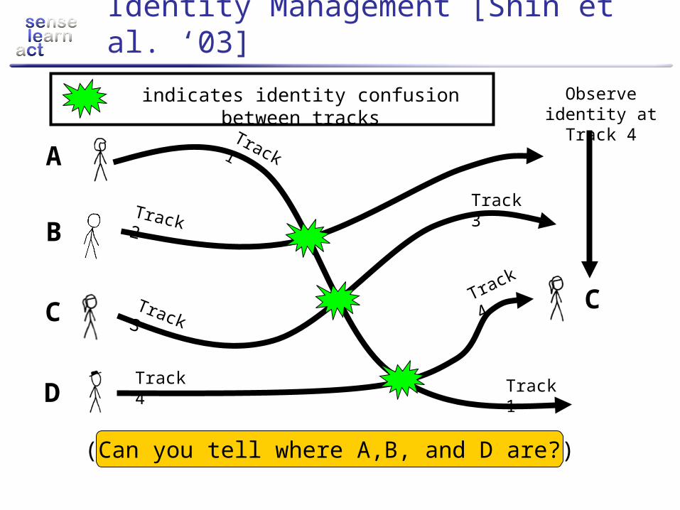
Reasoning with Permutations
We model uncertainty in identity management with distributions over permutations
A B C D
Tra
ck p
erm
uta
tion
s
Identities
Probability of each track
permutation
1 2 3 4
2 1 3 4
1 3 2 4
3 1 2 4
2 3 1 4
3 2 1 4
1 2 4 3
2 1 4 3
0
0
1/10
0
1/20
1/5
0
0
“Alice is at Track 1, and Bob is at Track 3,
and Cathy is at Track 2,and David is at Track 4with probability 1/10”
P()

How many permutations?There are n! permutations!
Graphical models not appropriate due to mutual exclusivity constraints which lead to a fully connected graph
If A is in Track 1, then B cannot be in Track 1
n n! Memory required to store n! doubles
9 362,880 3 megabytes
12 4.8x10⁸ 9.5 terabytes
15 1.31x101
2
1729 petabytes
24 6.2x10²³ 4.5x10¹² petabytesAvogadro’s
Number

ObjectivesPermutations appear in many real world problems!
Identity Management / Data AssociationCard Shuffling AnalysisRankings and Voting Analysis
We will:Find a principled, compact representation for distributions over permutations with tuneable approximation qualityReformulate Hidden Markov Model inference operations with respect to our new representation:
MarginalizationConditioning

1st order summariesAn idea: store marginal probabilities that identity j maps to track i
A B C D
Tra
ck p
erm
uta
tion
s
Identities
1 2 3 4
2 1 3 4
1 3 2 4
3 1 2 4
2 3 1 4
3 2 1 4
1 2 4 3
2 1 4 3
0
0
1/10
0
1/20
1/5
0
0
“David is at Track 4with probability:
=1/10+1/20+1/5=7/20 ”
P()

1st order summariesWe can summarize a distribution using a matrix of 1st order marginalsRequires storing only n2 numbers!Example:
3/10 0 1/2 1/5
1/5 1/2 3/10 0
3/10 1/5 1/20 9/20
1/5 3/10 3/20 7/20
A B C D
1
2
3
4
Identities
Tra
cks
“Cathy is at Track 3 with probability 1/20”
“Bob is at Track 2 with zero probability”

The problem with 1st order
What 1st order summaries can capture:P(Alice is at Track 1) = 3/5 P(Bob is at Track 2) = 1/2
Now suppose:Tracks 1 and 2 are close, and Alice and Bob are not next to each other…Then P({Alice,Bob} occupy Tracks{1,2}) = 0
Moral: 1st order summaries cannot capture higher order dependencies!
Unordered Pairs

2nd order summariesIdea #2: store marginal probabilities that identities {k,l} map to tracks {i,j}
A B C D
Tra
ck p
erm
uta
tion
s
Identities
1 2 3 4
2 1 3 4
1 3 2 4
3 1 2 4
2 3 1 4
3 2 1 4
1 2 4 3
2 1 4 3
0
0
1/10
0
1/20
1/5
0
0
“Alice and Bob occupy Tracks 1 and 2 with zero
probability”
P()
Requires storing O(n4) numbers – one for each pair of unordered pairs, ({i,j},{k,l})

Et cetera…And so forth… We can define:
3rd-order marginals
4th-order marginals … nth-order marginals (which recovers the original distribution but requires n! numbers)
Fundamental Trade-off: we can capture higher-order dependencies at the cost of storing more numbers
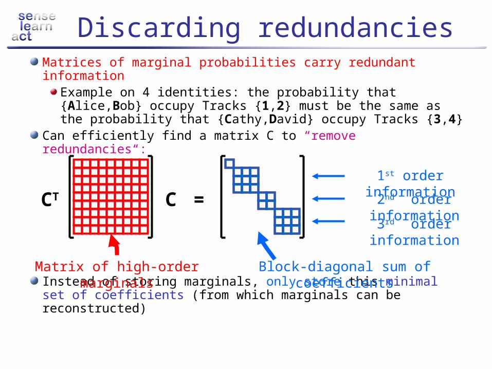
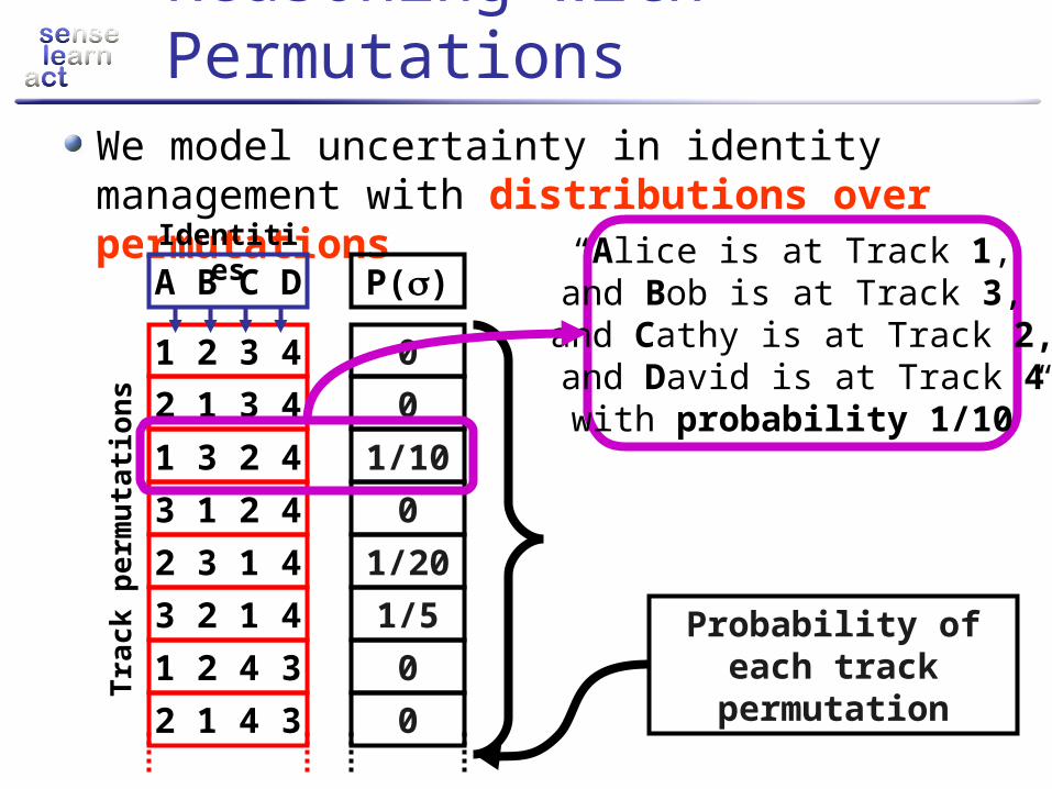
Discarding redundanciesMatrices of marginal probabilities carry redundant information
Example on 4 identities: the probability that {Alice,Bob} occupy Tracks {1,2} must be the same as the probability that {Cathy,David} occupy Tracks {3,4}
Can efficiently find a matrix C to “remove redundancies“:
Instead of storing marginals, only store this minimal set of coefficients (from which marginals can be reconstructed)
CT C =
Matrix of high-order marginals
Block-diagonal sum of coefficients
1st order information2nd order information3rd order
information

The Fourier viewOur minimal set of coefficients can be interpreted as a generalized Fourier basis!! [Diaconis, ‘88]General picture provided by group theory:
The space of functions on a group can be decomposed into Fourier components with the familiar properties: Orthogonality, Plancherel’s theorem, Convolution theorem, …
For permutations, simple marginals are “low-frequency”:
1st order marginals are “lowest-frequency” basis functions2nd order (unordered) marginals are 2nd lowest-frequency basis functions…

Group representationsThe analog of sinusoidal basis functions for groups are called group representationsA group representation, of a group G is a map from G to the set of d d matrices such that for all , G:
Example: The trivial representation ¿0 is defined by:
¿0 is the constant basis function and captures the normalization constant of a distribution in the generalized Fourier theory
This is like:
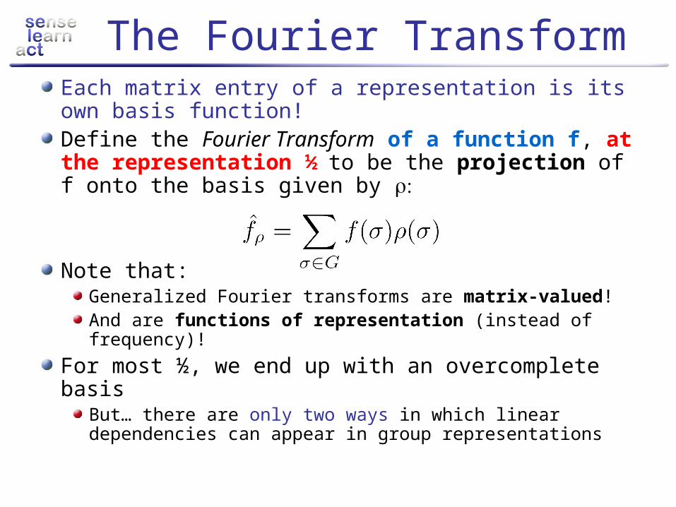
The Fourier TransformEach matrix entry of a representation is its own basis function!Define the Fourier Transform of a function f, at the representation ½to be the projection of f onto the basis given by
Note that:Generalized Fourier transforms are matrix-valued!And are functions of representation (instead of frequency)!
For most ½, we end up with an overcomplete basisBut… there are only two ways in which linear dependencies can appear in group representations
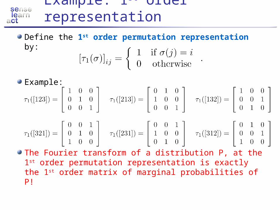
Example: 1st order representation
Define the 1st order permutation representation by:
Example:
The Fourier transform of a distribution P, at the 1st order permutation representation is exactly the 1st order matrix of marginal probabilities of P!

Two sources of overcompleteness
1. Can combine two representations, , to get a new representation (called the direct sum representation):
Example: (direct sum of two trivial representations)
2. Given a representation ½1, can “change the basis” to get a new representation by conjugating with an invertible matrix, C:
½1 and ½2 are called equivalent representations
Dealing with overcompleteness
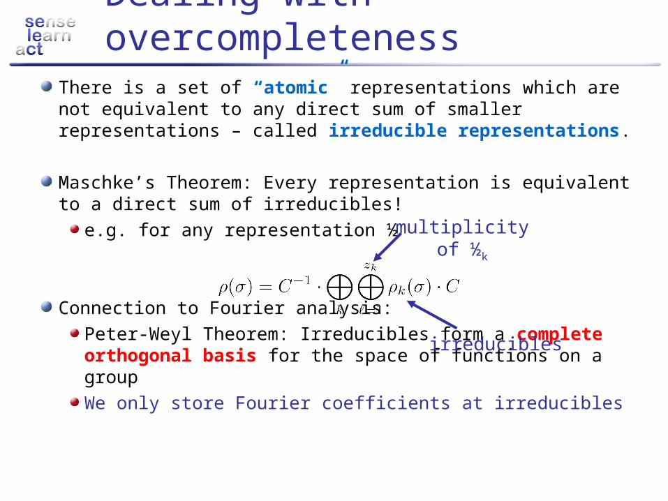
There is a set of “atomic” representations which are not equivalent to any direct sum of smaller representations – called irreducible representations.
Maschke’s Theorem: Every representation is equivalent to a direct sum of irreducibles!
e.g. for any representation ½
Connection to Fourier analysis:Peter-Weyl Theorem: Irreducibles form a complete orthogonal basis for the space of functions on a groupWe only store Fourier coefficients at irreducibles
irreducibles
multiplicity of ½k

Hidden Markov model inference
Prediction/Rollup:
Conditioning:
1 2 3 4
z1 z2 z3 z4
Latent Permutations
Identity Observations
Problem Statement: For each timestep, return posterior marginal probabilities conditioned on all past observationsTo do inference using Fourier coefficients, we need to cast all inference operations in the Fourier domain
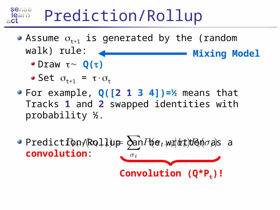
Prediction/RollupAssume t+1 is generated by the (random walk) rule:
Draw Q()Set t+1 = t
For example, Q([2 1 3 4])=½ means that Tracks 1 and 2 swapped identities with probability ½.
Prediction/Rollup can be written as a convolution:
Mixing Model
Convolution (Q*Pt)!

Fourier Domain Prediction/Rollup
Convolutions are pointwise products in the Fourier domain!
Can update individual frequency components independently:Update rule: for each irreducible ½:
Fourier domain Prediction/Rollup is exact on the maintained Fourier components!
matrix multiplication

ConditioningBayes rule is a pointwise product of the likelihood function and prior distribution:
Example likelihood function: P(z=green | ¾(Alice)=Track 1) = 9/10(“If Alice is at Track 1, then we see green at Track 1 with probability 9/10”)
PriorPosteriorLikelihood
Track 1
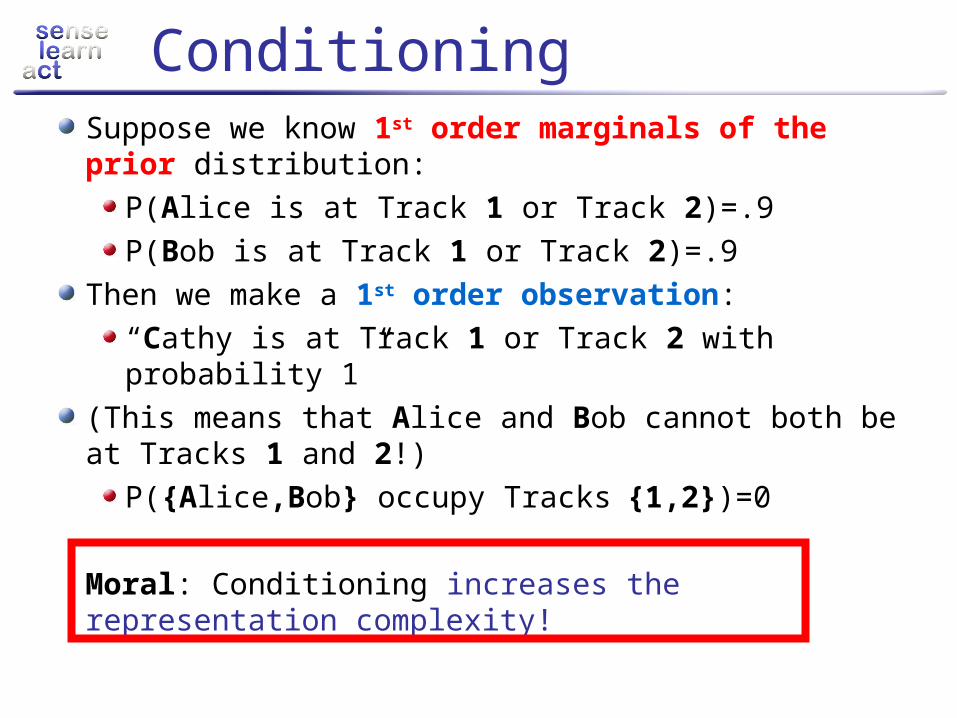
ConditioningSuppose we know 1st order marginals of the prior distribution:
P(Alice is at Track 1 or Track 2)=.9P(Bob is at Track 1 or Track 2)=.9
Then we make a 1st order observation: “Cathy is at Track 1 or Track 2 with probability 1”
(This means that Alice and Bob cannot both be at Tracks 1 and 2!)
P({Alice,Bob} occupy Tracks{1,2})=0
Moral: Conditioning increases the representation complexity!
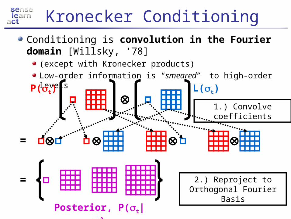
Kronecker ConditioningConditioning is convolution in the Fourier domain [Willsky, ‘78]
(except with Kronecker products)Low-order information is “smeared” to high-order levels
P(t) L(t)
=
= 2.) Reproject to Orthogonal Fourier Basis
Posterior, P(t|z)
1.) Convolve coefficients
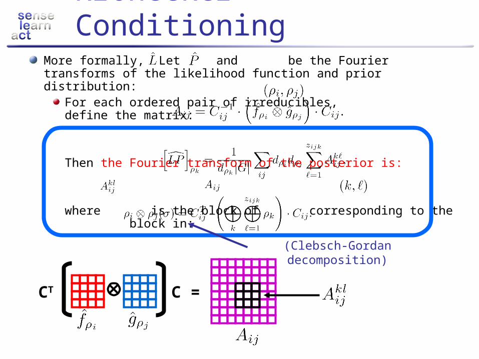
Kronecker ConditioningMore formally, Let and be the Fourier transforms of the likelihood function and prior distribution:
For each ordered pair of irreducibles, define the matrix:
Then the Fourier transform of the posterior is:
where is the block of corresponding to the block in:
(Clebsch-Gordan decomposition)
CT C =

Bandlimiting and error analysis
For tractability, discard “high-frequency” coefficients
Equivalently, maintain low-order marginalsFourier domain Prediction/Rollup is exactKronecker Conditioning introduces errorBut if we have enough coefficients, then Kronecker conditioning is exact at a subset of low-frequency terms!
Theorem. If the Kronecker Conditioning Algorithm is called using pth order terms of the prior and qth order terms of the likelihood, then the (|p-q|)th order marginals of the posterior can be reconstructed without error.

Dealing with negative numbers
Consecutive Conditioning steps propagates errors to all frequency levelsErrors can cause our marginal probabilities to be negative!Solution: Project to the Marginal Polytope (Fourier coefficients corresponding to nonnegative marginal probabilities)
Minimize the distance to the Marginal Polytope in the Fourier domain by using the Plancherel theorem:
Minimization can be written as an efficient Quadratic program!

Algorithm summaryInitialize prior Fourier coefficient matricesFor each timestep t = 1,2,…,T
Prediction/Rollup:For all coefficient matrices
Conditioning
For all pairs of coefficient matrices Compute and reproject to the orthogonal Fourier basis using the Clebsch-Gordan decomposition
Drop high frequency coefficients ofProject to the Marginal polytope using a Quadratic program
Return marginal probabilities for all timesteps

Simulated data drawn from HMM
Accuracy of Kronecker Conditioning after
several mixings (n=8)Running Time for
processing 10 timesteps
Measured at 1st order marginals
2nd order (ordered)
2nd order (unordered)
1st order
Exact inference
(Keeping all 2nd order marginals is enough to ensure zero error for 1st
order marginals)
Bett
er
Bett
er
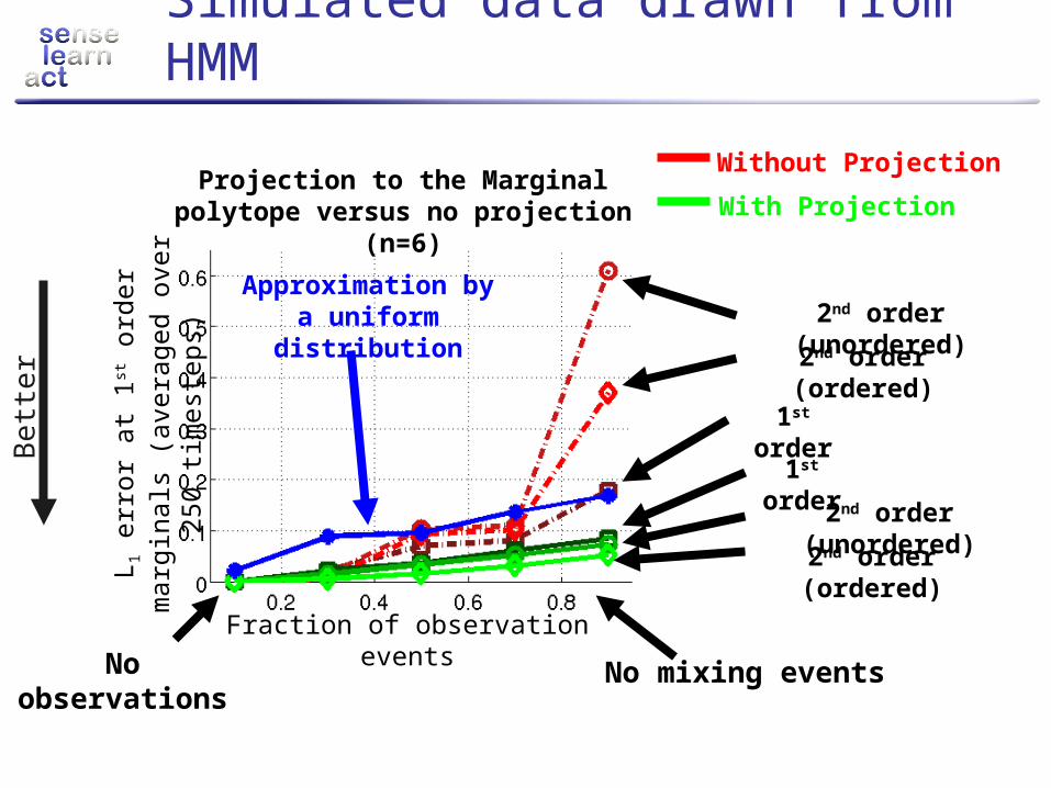
Simulated data drawn from HMM
Fraction of observation events
L 1 e
rror
at
1st o
rder
marg
inals
(a
vera
ged o
ver
250 t
imest
eps)
Projection to the Marginal polytope versus no projection
(n=6)With Projection
Without Projection
1st order
2nd order (ordered)
2nd order (unordered)
Approximation by a uniform
distribution
1st order
2nd order (ordered)
2nd order (unordered)
No mixing eventsNo observations
Bett
er
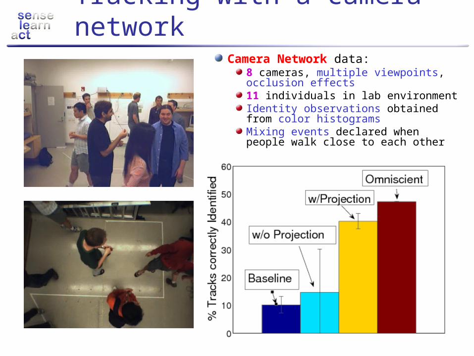
Tracking with a camera network
Camera Network data:8 cameras, multiple viewpoints, occlusion effects11 individuals in lab environmentIdentity observations obtained from color histogramsMixing events declared when people walk close to each other

ConclusionsPresented an intuitive, principled representation for distributions on permutations with
Fourier-analytic interpretations, andTuneable approximation quality
Formulated general and efficient inference operations directly in the Fourier DomainAnalyzed sources of error which can be introduced by bandlimiting and showed how to combat them by projecting to the marginal polytopeEvaluated approach on real camera network application and simulated data