Embed Size (px)
Citation preview
8/3/2019 Carlo R. Laing- On the application of "equation-free" modelling to neural systems
http://slidepdf.com/reader/full/carlo-r-laing-on-the-application-of-equation-free-modelling-to-neural-systems 1/34
On the application of “equation-free” modelling to neural systems
Carlo R. Laing ( ¡ £ ¡ ¦ ¨ ¨ ! ! # % ¡ ¢ ¡ ) )0
Institute of Information and Mathematical Sciences, Massey University, Auckland, New Zealand
July 26, 2005
Abstract. “Equation-free modelling” is a recently-developed technique for bridging the gap between detailed,microscopic descriptions of systems and macroscopic descriptions of their collective behaviour. It uses short,repeated bursts of simulation of the microscopic dynamics to analyse the effective macroscopic equations, eventhough such equations are not directly available for evaluation. This paper demonstrates these techniques ona variety of networks of model neurons, and discusses the advantages and limitations of such an approach.New results include an understanding of the effects of including gap junctions in a model capable of sustainingspatially localised “bumps” of activity, and an investigation of a network of coupled bursting neurons.
1. Introduction
Many physical systems involve the interaction of many “units” — particles, cells, molecules,random walkers, etc. — and the equations governing the local dynamics of these units andthe interactions between them are often known in some detail. Many of these systems have“emergent” macroscopic behaviour, such as a convective roll in a fluid heated from below.Often, it is this behaviour that is of interest to us, rather than the detailed behaviour of the many individual units (water molecules, in this example). For some systems such as
fluid flow, we can construct approximate equations that govern the macroscopic dynamicsand work directly with them, ignoring the microscopic details. This is appropriate if weare interested in phenomena that occur on much larger spatial scales, and much longertime-scales, than those associated with individual molecules.
However, for many systems of interest it is not possible to derive such macroscopicequations. Equation-free (EF) modelling, developed in the past few years by Kevrekidis etal. (Gear et al., 2002; Kevrekidis et al., 2003; Makeev et al., 2002; Moller et al., 2005; Runborget al., 2002), is a way of analysing the macroscopic equations for such a system, eventhough the equations are not known explicitly, by using short bursts of appropriately-initialised simulations of the microscopic dynamics. Its success relies on there being aseparation of time-scales in the system, with the macroscopic variables of interest changing
on a much longer time-scale than most of the microscopic variables. It is computationallyintensive, with repeated simulations of often highly-detailed models on a microscopic level
being required; this makes them amenable to implementation on parallel computers. Theidea is similar to that of approximate inertial manifolds in the analysis of partial differentialequations (Garcia-Archilla et al., 1998), where the amplitudes of higher modes (which,for example, have rapid spatial variation) are “slaved” to (or are functions of) the ampli-tudes of a finite number of lower modes (which, for example have slow spatial variation).Thus a simulation of the lower modes, together with knowledge of the slaving relation-ship, is sufficient to give an accurate description of the solutions of the whole PDE. For a
broader overview of the problem of extracting macroscopic dynamics from a microscopicdescription of a system, see Givon et al. (2004).
1
Corresponding author.
c2
2005 Kluwer Academic Publishers. Printed in the Netherlands.
3 4 6 8 @ 3 B C D F 4 H P Q S T U V T Q U U X P Y Q a Q S P c D Y

8/3/2019 Carlo R. Laing- On the application of "equation-free" modelling to neural systems
http://slidepdf.com/reader/full/carlo-r-laing-on-the-application-of-equation-free-modelling-to-neural-systems 2/34
2 Laing
The ideas involving in EF modelling have previously been implemented for a variety
of different problems; for example, a Lattice-Boltzmann implementation of the FitzHugh-Nagumo PDE in one spatial dimension (Gear et al., 2002), and kinetic Monte Carlo modelsof simple chemical reactions on a surface (Makeev et al., 2002). The purpose of this paper isto demonstrate in detail the EF modelling of several different networks of model neurons.As will be seen, some of the results could have been obtained by different methods, butsome new results that could not be obtained by other methods will also be shown. Theemphasis here is on an exposition of the techniques rather than the novel results.
Neural systems are suitable for this type of analysis for several reasons. One is that neu-ral systems normally have a wide range of time-scales, which is a crucial requirement forthe ideas discussed here to work. For example, spike frequency adaptation normally occurson a much longer time-scale than the processes involved in the generation of a single action
potential. Another reason is the wide range in the level of description of various neuralsystems, from single ion channels to much larger ensembles of neurons (Koch, 1999) andultimately, brain regions. While a specific system may be well understood at a particularlevel of description, it is often hard to integrate that system into a larger one without mak-ing drastic simplifications. For example, while a single neuron may be well-characterisedin terms of the ion channels involved in its action potential generation, often that detailis thrown away when a network of such neurons is studied, and only the frequency of firing for a fixed input is considered. For the examples we study, we can include as muchdetail as is known in the description of the dynamics of individual neurons (keeping thesingle neuron model in a “black box” to be simulated when necessary) but we can stilldescribe the behaviour of a network of neurons in terms of a small number of macroscopicvariables.
The structure of the paper is as follows. We now give a brief introduction to EF mod-elling; much more detail can be found elsewhere (Gear et al., 2002; Kevrekidis et al., 2003;Makeev et al., 2002; Moller et al., 2005; Runborg et al., 2002). In Sec. 2 we discuss a simplenetwork of model neurons, all-to-all coupled with slow excitatory coupling. In Sec. 3 westudy two populations that mutually inhibit one another; this leads to bistability. In Sec. 4we investigate a system capable of supporting spatial patterns, while Sec. 5 discusses anetwork of bursting neurons, and in Sec. 6 we study a noisy network. We conclude inSec. 7.
Equation-free modellingConsider numerical integration in time, or simulation, of a complex system whose micro-scopic dynamics one knows in detail. An example is a network of coupled neurons. Let U
be the macroscopic variable that one hopes describes the system (for example, an averagerate of firing), and let u be the vector-valued variable describing the microscopic state of the system (for example, a vector containing the voltages and gating variables of all of the neurons in the network). u is normally much higher-dimensional than U. We supposethat there exists a function F(U) such that the dynamics of U are given by the differentialequation
dU
dt F(U) (1)
We do not have an explicit formula for F(U) and cannot evaluate it in the usual sense of a function evaluation, but we assume that F(U) exists and is well-behaved (for example,
that it is differentiable). We also assume that U changes slowly in time relative to the rate
3 4 6 8 @ 3 B C D F 4 H P Q S T U V T Q U U X P Y Q a Q S P c D Q
8/3/2019 Carlo R. Laing- On the application of "equation-free" modelling to neural systems
http://slidepdf.com/reader/full/carlo-r-laing-on-the-application-of-equation-free-modelling-to-neural-systems 3/34
Equation-free modelling 3
of change of most of the components of u Suppose that we want to make an Euler step
forward in time, from an initial condition U0, i.e. we know the state of U now, and want toknow it at a small time h in the future. The formula is
U1 U0
¡
hF(U0) (2)
where U1 is the value of U at time t h, and h is the time-step we have chosen. To evaluateF(U0) we initialise the microscopic system (the full network) with an initial condition u0
that is consistent with U having the value U0. This is done with a “lifting” operator, M,such that u0
MU0. This is a one-to-many operation, as there are generally an infinitenumber of initial conditions for the microscopic system that are consistent with U having aparticular value. We typically do this by choosing u0 from a conditional probability densityfunction p(u0
¢
U0). We also have a “restricting” operator, m, which extracts the value of U,
given u, i.e. U
mu. This is normally a many-to-one operator, and could be as simple astaking an average. The operators M and m satisfy mM I , the identity, so that lifting andthen immediately restricting should have no effect, within roundoff error.
We then run the microscopic system for a short amount of time,£
. During this timethe quickly-changing components of u vary so that the probability density function of u
becomes “slaved” to (or determined by) the current value of U (Kevrekidis et al., 2003). LetU
¤
mu¢
t¥
¤, i.e. the restriction of u after a time
£. We then run the microscopic simulation
for a further time ∆t. This time is long enough for U to change appreciably, but not solong that nonlinear effects appear in its behaviour, i.e. over the time interval [
£ ¦ £
¡
∆t], Ushould change approximately linearly with time. We then use a simple forward difference
U¤ ©
∆t
U¤
∆t (3)
as an approximation todU
dt
U¥
U0
(4)
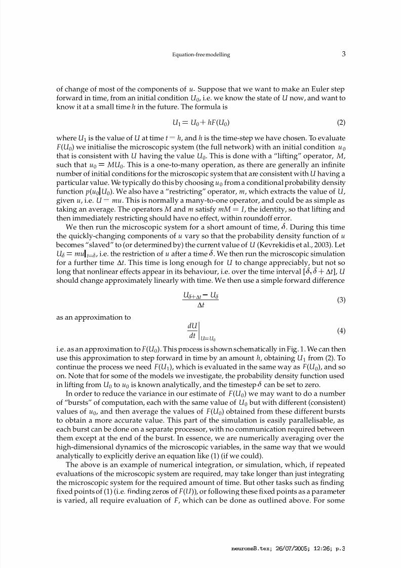
i.e. as an approximation to F(U0). This process is shown schematically in Fig. 1. We can thenuse this approximation to step forward in time by an amount h, obtaining U1 from (2). Tocontinue the process we need F(U1), which is evaluated in the same way as F(U0), and soon. Note that for some of the models we investigate, the probability density function usedin lifting from U0 to u0 is known analytically, and the timestep
£can be set to zero.
In order to reduce the variance in our estimate of F(U0) we may want to do a number
of “bursts” of computation, each with the same value of U0 but with different (consistent)values of u0, and then average the values of F(U0) obtained from these different burststo obtain a more accurate value. This part of the simulation is easily parallelisable, aseach burst can be done on a separate processor, with no communication required betweenthem except at the end of the burst. In essence, we are numerically averaging over thehigh-dimensional dynamics of the microscopic variables, in the same way that we wouldanalytically to explicitly derive an equation like (1) (if we could).
The above is an example of numerical integration, or simulation, which, if repeatedevaluations of the microscopic system are required, may take longer than just integratingthe microscopic system for the required amount of time. But other tasks such as findingfixed points of (1) (i.e. finding zeros of F(U)), or following these fixed points as a parameter
is varied, all require evaluation of F, which can be done as outlined above. For some
3 4 6 8 @ 3 B C D F 4 H P Q S T U V T Q U U X P Y Q a Q S P c D
8/3/2019 Carlo R. Laing- On the application of "equation-free" modelling to neural systems
http://slidepdf.com/reader/full/carlo-r-laing-on-the-application-of-equation-free-modelling-to-neural-systems 4/34
4 Laing
Time
U
δ
∆ t
Figure 1. A schematic diagram showing the time
, during which the fast variables become “slaved” to theslow ones, and the time ∆t, during which the change in U is determined. The thick line represents the trueevolution of U, while the jagged line represents the restriction mu from one particular realisation of themicroscopic dynamics. In this case, u was not initialised with a value consistent with the true value of U(0),hence the difference in initial conditions. See Sec. 1 for more detail.
of these tasks, evaluation of derivatives of F with respect to variables or parameters areneeded. These can be approximated through finite differences, i.e. through running themicroscopic system with nearby initial conditions, or at slightly different parameter values.It is this ability to simulate the microscopic system at will with specific initial conditions(which is either very difficult or impossible for a physical system) that is exploited in theEF modelling paradigm.
2. One population, positive feedback
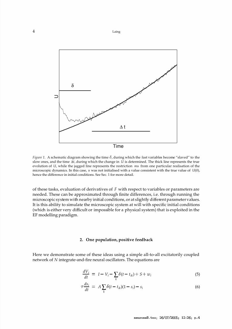
Here we demonstrate some of these ideas using a simple all-to-all excitatorily couplednetwork of N integrate-and-fire neural oscillators. The equations are
dV idt
I
V i ∑
k
£(t
tik)¡
S¡
wi (5)
¡
dsi
dt
A∑k£
(t
tik)(1
si)
si (6)
3 4 6 8 @ 3 B C D F 4 H P Q S T U V T Q U U X P Y Q a Q S P c D ¢
8/3/2019 Carlo R. Laing- On the application of "equation-free" modelling to neural systems
http://slidepdf.com/reader/full/carlo-r-laing-on-the-application-of-equation-free-modelling-to-neural-systems 5/34
Equation-free modelling 5
for i 1¦
N , where tik is the kth firing time of neuron i (defined to be the times at which
V i reaches 1 from below), S is the average of the si,
S
1
N
N
∑i
¥ 1
si (7)
and the sums over k are over all past firing times. V i is the voltage of neuron i and lies in[0
¦1), si is the strength of the synapses leaving neuron i, I is a constant input current and A
controls the overall strength of synapses. The function£
(¡) is the Dirac delta function, used
to reset the V i to zero, and increment the si upon firing. The variables wi are independentGaussian white noise terms, with properties
¢
wi(t)£
0¢
wi(t)wi(s)£
¤2
£(t
s) (8)
for each i, where the angled brackets indicate averages. The parameter¤
controls the noiseintensity. Noise was added to this system to smooth out the function describing the firingfrequency of a single neuron as a function of its input current, which is known not to
be differentiable everywhere for type I neurons, of which the integrate-and-fire neuron isan example (Gerstner and Kistler, 2002). This enables continuation algorithms, which relyon functions being sufficiently differentiable, to be used, and also makes the model more
biologically realistic.To ensure a separation of timescales, ¡ is chosen to be 50, which is large relative to the
timescale of changes in voltage (i.e. we have slow synapses). In the absence of coupling( A 0), each model neuron behaves like an independent integrate-and-fire neuron, witha noisy input. When A is not zero, the neurons are coupled through the average of the s i.
Each time neuron i fires, si is increased by an amount A(1 si)¦
¡
; in between firing timessi undergoes exponential decay back to zero with time constant ¡ . For a range of valuesof I , the system (5)-(6) is attracted to a state where all neurons are firing approximatelyperiodically and are not synchronised.
For this system the vector u describing the microscopic state of the network would beformed from all of the V i and si. Using the EF modelling approach, we assume that exactvalues of all of these variables are not of interest, in terms of describing the state of thenetwork, Instead, the assumption is that the single variable S characterises the dynamicsof the system, and that there is a single equation governing the dynamics of S, say
dS
dt F(S; I ) (9)
Thus for this system, the macroscopic variable U is just S. It should be stressed that it is anassumption that the behaviour of the network (5)-(6) can be accurately described by (9).
In order to perform numerical bifurcation analysis of (9) we need to be able to evaluateF(S; I ) and its partial derivatives with respect to both S and I . To evaluate F(S; I ) werun (5)-(6) for a short amount of time and monitor S during that integration. The integration must
be long enough for S to change appreciably and for the V i to redistribute (if necessary) sothat their probability density function is appropriate for the current value of S (i.e. for thesystem to “heal” (Gear et al., 2002)), but not so long that nonlinear effects start to come intoplay, since nonlinear effects will reduce the validity of the approximation (3). The correctintegration time can be determined by running a number of simulations and observing thedifferent time-scales in the dynamics. Alternatively, for a system like (5)-(6), we can use the
explicitly-given slow time-scale, ¡ , to choose the integration time, setting it to, say, ¡
¦ 2.
3 4 6 8 @ 3 B C D F 4 H P Q S T U V T Q U U X P Y Q a Q S P c D X
8/3/2019 Carlo R. Laing- On the application of "equation-free" modelling to neural systems
http://slidepdf.com/reader/full/carlo-r-laing-on-the-application-of-equation-free-modelling-to-neural-systems 6/34
6 Laing
2.1. INITIAL CONDITIONS
The question of initial conditions must be addressed. From a particular value of S we needto generate 2N initial conditions, for the V i and si. In principle, since S is the average of thesi, we could choose the si(0) from any distribution with mean S. For simplicity, we choosesi(0) S for all i. (This is one component of our lifting operator, M; the restricting operatoris just the averaging of the si.) Also in principle, the V i(0) could be chosen in any way fromthe interval [0
¦1). However, there are some points to be considered.
If all V i(0) are chosen to be equal then the neurons will start off synchronised, since allsi(0) are equal to one another as well. The nonzero noise intensity will break up this syn-chronisation, but we need this to occur well before the end of the short burst of simulation.A better choice would be to take the V i(0) from a uniform distribution over [0
¦
1). Thiswould remove the problem of synchronisation but it is still not the best solution. A mo-ment’s thought shows that during periodic firing the V i are not spread uniformly throughthe interval [0
¦1) but are more likely to be near 1 than near 0. In fact, if ¤ 0 (i.e. the noise
intensity is zero), the probability density function (PDF) for the V i is p(V i¢
I ¡
S), where
p(V i¢
I )
1B(I ¡ V i)
if I ¢
1
£(V i
I ) if I £
1(10)
where B log[I ¦
(I
1)]. When ¤ ¤ 0 it is also possible to calculate the PDF for theV i (Brunel and Hakim, 1999; Fourcaud and Brunel, 2002):
p(V i¢
I )
2 f 0¤
exp¦
(V i
I )2
¤
2§ ¨
(1 ¡
I )
¡I
exp(s2) ds if V i £0
(1¡
I )
(V i ¡I )
exp(s2) ds if V i ¢ 0(11)
where f 0 is the stationary firing rate:
f 0
¦ ! "
(1 ¡
I )
¡I
exp$
x2 % [1¡
erf(x)]dx§
¡ 1
(12)
and erf is the error function. We will use the PDF given by (10), rather than (11), for threereasons. Firstly, there are difficulties with numerically implementing (11) when ¤ ¤ 0,due to overflow errors. Secondly, the difference between the PDFs (10) and (11) is onlysignificant when I
¡
S'
1. Thirdly, due to the difference in timescales for the V i and si, asmentioned above, the initial conditions for the V
iare largely irrelevant.
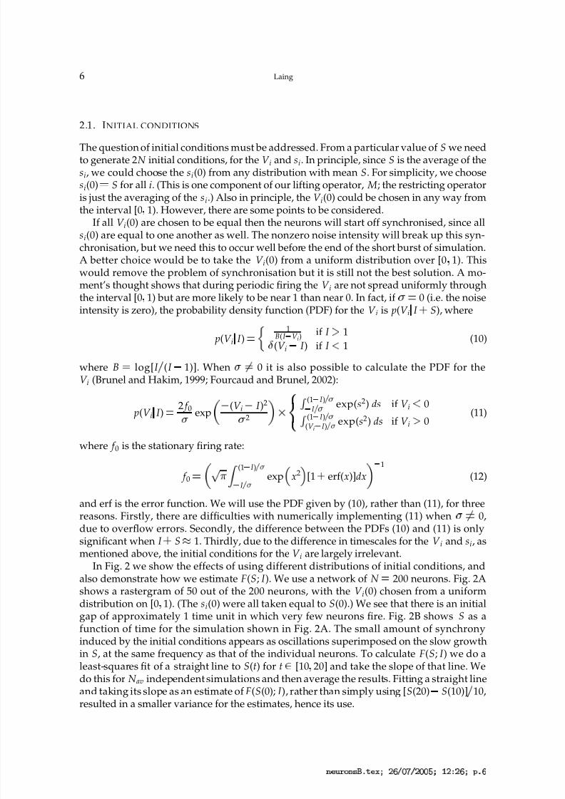
In Fig. 2 we show the effects of using different distributions of initial conditions, andalso demonstrate how we estimate F(S; I ). We use a network of N 200 neurons. Fig. 2Ashows a rastergram of 50 out of the 200 neurons, with the V i(0) chosen from a uniformdistribution on [0
¦1). (The si(0) were all taken equal to S(0).) We see that there is an initial
gap of approximately 1 time unit in which very few neurons fire. Fig. 2B shows S as afunction of time for the simulation shown in Fig. 2A. The small amount of synchronyinduced by the initial conditions appears as oscillations superimposed on the slow growthin S, at the same frequency as that of the individual neurons. To calculate F(S; I ) we do aleast-squares fit of a straight line to S(t) for t
([10
¦20] and take the slope of that line. We
do this for N av independent simulations and then average the results. Fitting a straight lineand taking its slope as an estimate of F(S(0); I ), rather than simply using [S(20)
S(10)]¦
10,
resulted in a smaller variance for the estimates, hence its use.
3 4 6 8 @ 3 B C D F 4 H P Q S T U V T Q U U X P Y Q a Q S P c D S
8/3/2019 Carlo R. Laing- On the application of "equation-free" modelling to neural systems
http://slidepdf.com/reader/full/carlo-r-laing-on-the-application-of-equation-free-modelling-to-neural-systems 7/34
Equation-free modelling 7
0 5 10 15 200.162
0.164
0.166
0.168
Time
S
D
C
2 4 6 8 10 12 14 16 18 20
10
20
30
40
50
0 5 10 15 200.162
0.164
0.166
0.168
S
B
A
2 4 6 8 10 12 14 16 18 20
10
20
30
40
50
Figure 2. Demonstration of the effects of different probability density functions for the V i(0), for the sys-tem (5)-(6). A: A rastergram showing the firing times of 50 out of 200 neurons (vertical scale: neuron index).The V i(0) were randomly chosen from a uniform distribution on [0 1). B: S (the mean of the si) as a functionof time for the simulation in A. Also shown is the straight line (slope ¡ 1 40 £ 10 ¤
4) fitted to the second half of the simulation. C: Same as A, but with the V i(0) taken from the PDF (10). D: Same as B, but for the sim-ulation shown in C (slope ¡ 1 17 £ 10 ¤
4). Different realisations give qualitatively similar results (not shown).Parameters are S(0) ¡ 0 165 I ¡ 1. Other initial conditions are si(0) ¡ S(0) for i ¡ 1 N .
3 4 6 8 @ 3 B C D F 4 H P Q S T U V T Q U U X P Y Q a Q S P c D V
8/3/2019 Carlo R. Laing- On the application of "equation-free" modelling to neural systems
http://slidepdf.com/reader/full/carlo-r-laing-on-the-application-of-equation-free-modelling-to-neural-systems 8/34
8 Laing
0 0.05 0.1 0.15−8
−6
−4
−2
0
2
4
6
8
x 10−4
S
F ( S ; I )
I=0.91
I=0.93
I=0.95
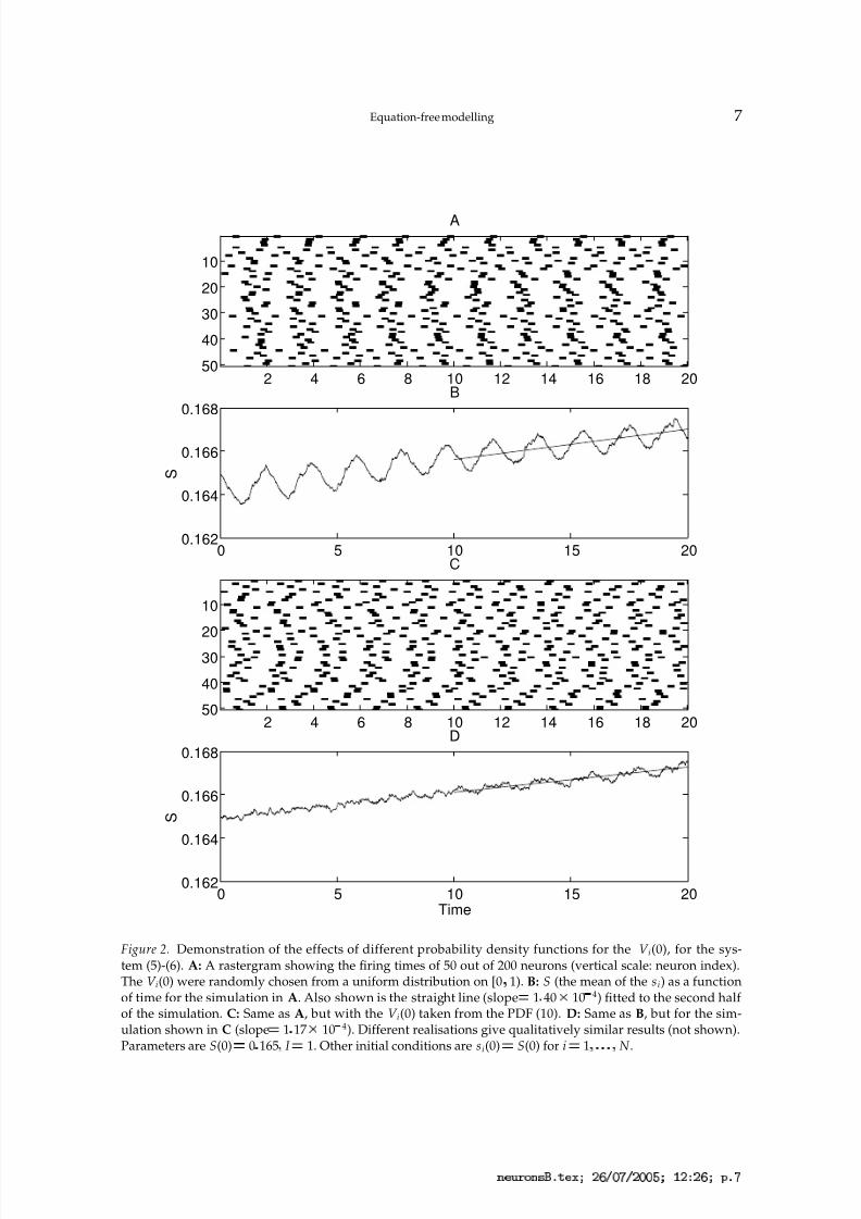
Figure 3. The function F(S; I ) (eqn. (9)), as calculated from direct simulation of (5)-(6), for three different valuesof I . Macroscopic fixed points occur when F(S; I ) ¡ 0. We have used a network of N ¡ 200 neurons, averagingover N av
¡ 30 realisations. Other parameters are A ¡ 0 4
¡ 50 ¡
¡ 0 0245.
Figure 2C shows a rastergram for 50 out of the 200 neurons when the V i(0) are chosenfrom the PDF given by (10). The lack of any synchrony is clear in Fig. 2D, where we plotS as a function of time for the simulation in Fig. 2C. Any oscillations seen here are due tothe noise and the fact that we do not have an infinite number of asynchronous neurons.Also shown in Fig. 2D is a least-squares fit of a straight line to S, as in Fig. 2B. The slope of this line differs from the slope in panel A by less than 20%. It is clear that other choices indetermining F(S; I ) are possible. For example, one could fit a straight line over a differenttime interval, or use S(20)
S(0), or fit a quadratic q(t) to S(t) and use q(20)
q(0), or anynumber of other possibilities.
This Figure also shows that S changes on a time scale much slower than that of theV i. Indeed, for this initial condition, the simulation must be run for 200 time units beforeS appears to saturate. This is expected, as each synaptic strength s i evolves with a timeconstant ¡
50.InFig. 3 we show F(S; I ) as a function of S, calculated as above, for three different values
of I . We again used a network of N 200 neurons, and averaged N av 30 times. We see
that for I 0 91, there is one stable fixed point very close to S 0 (it is stable, since F£
0for S
¢0). There are three fixed points for I 0 93 and only one, at a high value of S, for
I 0 95. We can see that there are some bifurcations of fixed points as I is varied. We now
discuss this.
3 4 6 8 @ 3 B C D F 4 H P Q S T U V T Q U U X P Y Q a Q S P c D £
8/3/2019 Carlo R. Laing- On the application of "equation-free" modelling to neural systems
http://slidepdf.com/reader/full/carlo-r-laing-on-the-application-of-equation-free-modelling-to-neural-systems 9/34
Equation-free modelling 9
0.9 0.92 0.94 0.96 0.98 10
0.02
0.04
0.06
0.08
0.1
0.12
0.14
0.16
0.18
I
S
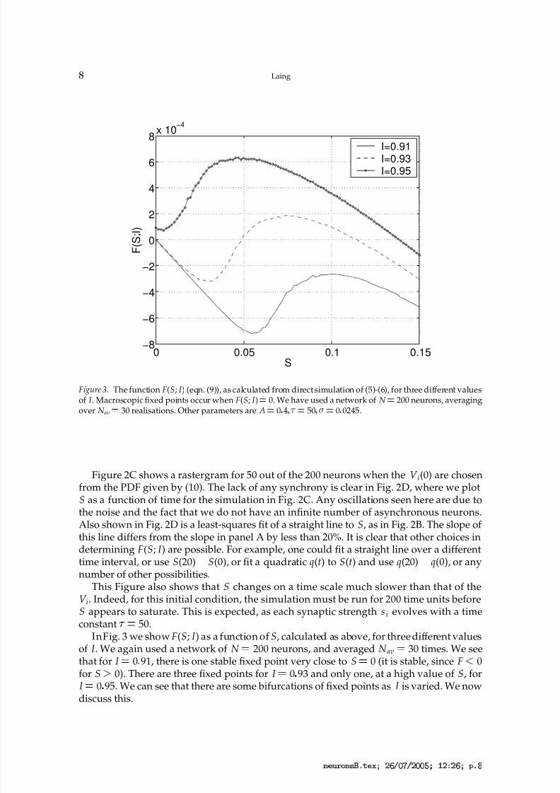
Figure 4. The curve of macroscopic steady states of the integrate-and-fire network (5)-(6) (points joined bya line). Parameters are A ¡ 0 4
¡ 50 ¡
¡ 0 0245. A network of N ¡ 200 was used, with averaging overN av
¡ 30 realisations. The dashed line shows the fixed points of the rate-based noise-free case [eqn. (15), with f given by (17)], while the solid line shows the solution of the rate-based system [eqn. (15), with f given
by (18)] with ¡
¡
0 0245.
2.2. FIXED POINTS
Figure 4 shows the curve of macroscopic fixed points for (5)-(6) as I is varied. These arefixed points of S, not of the microscopic variables (the V i and si). We have traced thiscurve using pseudo-arclength continuation (Doedel et al., 1991). Also shown in Fig. 4 aretwo curves that can be calculated analytically using a rate-based formulation, as we nowdiscuss.
Taking the average of the term ∑k £(t
tik) in Eqn. (6) over an interval of length T ,we obtain the number of times that neuron i has fired during that interval, divided by
T , i.e. the average firing rate of that neuron during that time interval. The neurons areidentical, each receiving an effective input current of I
¡
S. Thus each neuron will be firingat a rate f (I
¡
S), where f (I ) is the firing rate for a single integrate-and-fire neuron withinput I . Thus we can approximate (6) by
¡
dsidt
A f (I ¡
S)(1
si)
si i 1¦
¦ N (13)
Taking the average of these N equations we obtain one equation for S:
¡
dS
dt A f (I
¡
S)(1
S)
S (14)
Fixed points satisfy
g(S ¦ I ) 0 (15)
3 4 6 8 @ 3 B C D F 4 H P Q S T U V T Q U U X P Y Q a Q S P c D
8/3/2019 Carlo R. Laing- On the application of "equation-free" modelling to neural systems
http://slidepdf.com/reader/full/carlo-r-laing-on-the-application-of-equation-free-modelling-to-neural-systems 10/34
10 Laing
where
g(S ¦ I )
A f (I
¡
S)(1
S)
S¡ (16)
For a noise free neuron, i.e. when ¤ 0,
f (I ) f 1(I ) H (I
1)¦
log
I
I
1¡
§
¡ 1
(17)
where H is the Heaviside function. When ¤ ¤ 0,
f (I ) f 2(I )
¦ !"
b
aexp
$ x2 % [1¡
erf(x)]dx§
¡ 1
(18)
where a
I ¦
¤ , b (1
I )¦
¤ , and erf is the error function (Fourcaud and Brunel, 2002).Plotted in Fig. 4 are solutions of (15) where f (I ) is given by (17) (dashed line), and where
f (I ) is given by (18) (solid line). We see that for S greater than about 0 1, the three curvesare close. However, below the turning point the curve of macroscopic fixed points is much
better approximated by the curve for the rate-based model with the correct amount of noise, in the sense of the curves being closer to one another. The agreement between thesecurves is a useful confirmation that the method is working. We now discuss the stabilityof these fixed points.
2.3. STABILITY
The stability of a fixed point of (9) is given by the sign of ¢
F¦ ¢
S. A positive derivativeindicates instability, whereas a negative derivative indicates stability. A similar remark
holds for the rate-based equation, (15). To find the partial derivative of F(S; I ) with respectto its arguments we use finite differences. For example,
¢F
¢S
S¥S
'
F(S¡ ¤
; I )
F(S; I )¤
(19)
and similarly for¢ F ¦ ¢ I . In all following work we use a value of
¤
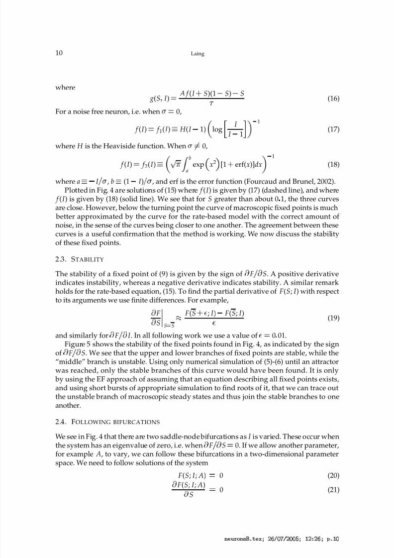
0 01.Figure 5 shows the stability of the fixed points found in Fig. 4, as indicated by the sign
of ¢ F ¦ ¢ S. We see that the upper and lower branches of fixed points are stable, while the
“middle” branch is unstable. Using only numerical simulation of (5)-(6) until an attractorwas reached, only the stable branches of this curve would have been found. It is only
by using the EF approach of assuming that an equation describing all fixed points exists,
and using short bursts of appropriate simulation to find roots of it, that we can trace outthe unstable branch of macroscopic steady states and thus join the stable branches to oneanother.
2.4. FOLLOWING BIFURCATIONS
We see in Fig. 4 that there are two saddle-node bifurcations as I is varied. These occur whenthe system has an eigenvalue of zero, i.e. when
¢F
¦ ¢S 0. If we allow another parameter,
for example A, to vary, we can follow these bifurcations in a two-dimensional parameterspace. We need to follow solutions of the system
F(S; I ; A) 0 (20)
¢
F(S; I ; A)¢ S
0 (21)
3 4 6 8 @ 3 B C D F 4 H P Q S T U V T Q U U X P Y Q a Q S P c D Y U
8/3/2019 Carlo R. Laing- On the application of "equation-free" modelling to neural systems
http://slidepdf.com/reader/full/carlo-r-laing-on-the-application-of-equation-free-modelling-to-neural-systems 11/34
Equation-free modelling 11
0.9 0.92 0.94 0.96 0.98 1−0.02
−0.01
0
0.01
0.02
0.03
0.04
I
E i g e n v a l u e
Figure 5. Eigenvalues for the steady states shown in Fig. 4. Positive values correspond to instability, negativeto stability. The points joined by a line are for macroscopic steady states of (5)-(6). The dashed line shows thestability for the rate-based noise-free case, while the solid line shows the stability for the rate-based systemwith ¡
¡ 0 0245.
where we have now explicitly included the dependence of F on A. Following solutionsto these equations requires more averaging (i.e. a much larger value of N av and/or N )to be successful, since we need to numerically estimate second derivatives of F duringcontinuation, not just first derivatives (Makeev et al., 2002).
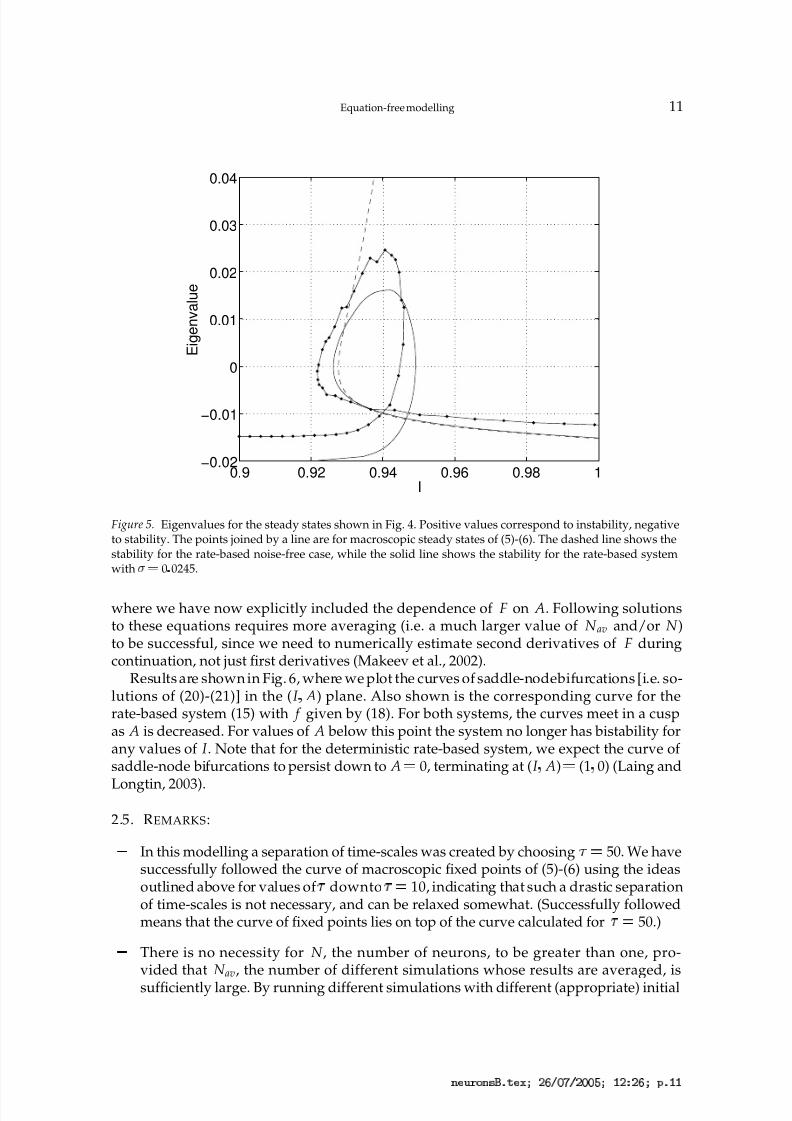
Results are shown in Fig. 6, where we plot the curves of saddle-nodebifurcations [i.e. so-lutions of (20)-(21)] in the (I
¦A) plane. Also shown is the corresponding curve for the
rate-based system (15) with f given by (18). For both systems, the curves meet in a cuspas A is decreased. For values of A below this point the system no longer has bistability forany values of I . Note that for the deterministic rate-based system, we expect the curve of saddle-node bifurcations to persist down to A 0, terminating at (I
¦A) (1
¦0) (Laing and
Longtin, 2003).
2.5. REMARKS:
In this modelling a separation of time-scales was created by choosing ¡
50. We havesuccessfully followed the curve of macroscopic fixed points of (5)-(6) using the ideasoutlined above for values of ¡ downto ¡
10, indicating that such a drastic separationof time-scales is not necessary, and can be relaxed somewhat. (Successfully followedmeans that the curve of fixed points lies on top of the curve calculated for ¡
50.)
There is no necessity for N , the number of neurons, to be greater than one, pro-vided that N av, the number of different simulations whose results are averaged, is
sufficiently large. By running different simulations with different (appropriate) initial
3 4 6 8 @ 3 B C D F 4 H P Q S T U V T Q U U X P Y Q a Q S P c D Y Y
8/3/2019 Carlo R. Laing- On the application of "equation-free" modelling to neural systems
http://slidepdf.com/reader/full/carlo-r-laing-on-the-application-of-equation-free-modelling-to-neural-systems 12/34
12 Laing
0.92 0.93 0.94 0.95 0.960.2
0.25
0.3
0.35
0.4
I
A
Figure 6. Solid line: the curve of saddle-node bifurcations of macroscopic steady states of the integrate-and-firenetwork (5)-(6). A network of N ¡ 1000 neurons was used, with averaging over N av
¡ 50 realisations. Otherparameters are
¡ 50 ¡
¡ 0 0245. Dashedline: the curve of saddle-node bifurcations for the rate-based systemwith ¡
¡ 0 0245. Figure 4 shows a horizontal “slice” through this figure at A ¡ 0 4.
conditions, we are still effectively sampling the whole space of microscopic variables.Having a larger N makes S more smooth, as it is the average of N variables, which inturn reduces the value of N av needed to obtain a reliable estimate of dS
¦dt.
In particular, the results obtained for N 1 are those that would be obtained if wehad a network of N identical neurons that were perfectly synchronised during the entire
burst of simulation. We return to this point in Sec. 7.
We also note that during the averaging we are performing, we are actually simultane-ously averaging over initial conditions for the V i and over realisations of the Gaussianwhite noise in (5).
As can be seen, there are a number of quantities that must be chosen, e.g. the numberof bursts to be averaged over (N av), and the lengths of the bursts. An element of trialand error may be involved in choosing these and it is possible that certain choices willcause the algorithms to break down. Verification of results through different means(for example, numerical simulation) may be prudent.
3 4 6 8 @ 3 B C D F 4 H P Q S T U V T Q U U X P Y Q a Q S P c D Y Q
8/3/2019 Carlo R. Laing- On the application of "equation-free" modelling to neural systems
http://slidepdf.com/reader/full/carlo-r-laing-on-the-application-of-equation-free-modelling-to-neural-systems 13/34
Equation-free modelling 13
3. Two mutually inhibiting populations
We now discuss a more complicated network of two distinct populations of identicalmodel integrate-and-fire neurons, each population inhibiting the other through the av-eraged synaptic activity.
3.1. THE MODEL
The equations are
dV 1idt
I 1
V 1i ∑k
£(t
t1ik)
S2 ¡
w1i (22)
dV 2idt
I 2
V 2i ∑k
£
(t
t2ik)
S1 ¡
w2i (23)
¡
ds1i
dt A∑
k
£(t
t1ik)(1
s1i )
s1i (24)
¡
ds2i
dt A∑
k
£(t
t2ik)(1
s2i )
s2i (25)
for 1¦
¦ N , where the superscripts identify the population,
S
p
1
N
N
∑i ¥ 1 s
p
i (26)
and the other terms have the same meanings as in the previous example. Note that all of the Gaussian white noise terms are independent.
For a fixed I 1 I 2¢
1 and A small, both populations will fire at the same rate. But for A large enough it is possible for one population to fire strongly, completely suppressingthe other in a “winner takes all” scenario. If I 1 I 2, this system is symmetric with respectto interchanging the populations, and we expect this symmetry to manifest itself in termsof the possible bifurcations that can occur. We again take ¡
50 to provide a separation of time scales.
Our assumption is that the dynamics are governed by the equations
dS1
dt F(S1
¦S2; A) (27)
dS2
dt F(S2
¦S1; A) (28)
where the same function F is used, due to the symmetry. We investigate these equationsin the same way as in the previous section. To evaluate F(S1
¦S2; A), we initialise each
s1i (0) S1 and s2
i (0) S2, and initialise the V 1i (0) using the PDF p(V 1i¢
I 1
S2) and theV 2i (0) using the PDF p(V 2i
¢
I 2
S1), where p is given by (10). We then integrate for 20time units and fit a straight line to S1(t) for 10
£t
£20 and take its slope — this is our
estimate of F(S1¦S2; A). Fitting another straight line to S2 over the same time interval gives
us an estimate of F(S2¦ S1; A). This procedure is repeated N av times with different initial
3 4 6 8 @ 3 B C D F 4 H P Q S T U V T Q U U X P Y Q a Q S P c D Y
8/3/2019 Carlo R. Laing- On the application of "equation-free" modelling to neural systems
http://slidepdf.com/reader/full/carlo-r-laing-on-the-application-of-equation-free-modelling-to-neural-systems 14/34
14 Laing
conditions for the voltages and different Gaussian white noise terms, and the results are
averaged.
3.2. RATE EQUATIONS
In a similar way to that in the previous section, we can write approximate rate equations forthe system (22)-(25), under the assumptions that we have an infinite number of perfectlyasynchronous neurons. The equations we obtain are
¡
dS1
dt A f (I 1
S2)(1
S1)
S1 (29)
¡
dS2
dt A f (I 2
S1)(1
S2)
S2 (30)
where f (I ) is the firing frequency of a neuron with input current I . We use the func-tion given by (18), with the same value of ¤ as that used in the simulations of (22)-(25).From (29)-(30) we see that when S1 S2, both of these values are given by the roots of
A f (I
S)(1
S)
S 0 (31)
whereas when S1 ¤ S2, all fixed points of (29)-(30) can be found by finding the roots of
A f ¦
I
A f (I
S)
1¡
A f (I
S) §
(1
S)
S 0 (32)
where I 1 I 2 I . The stability of these fixed points is determined by the eigenvalues of
the Jacobian of (29)-(30), evaluated at the fixed points.
3.3. NUMERICAL RESULTS
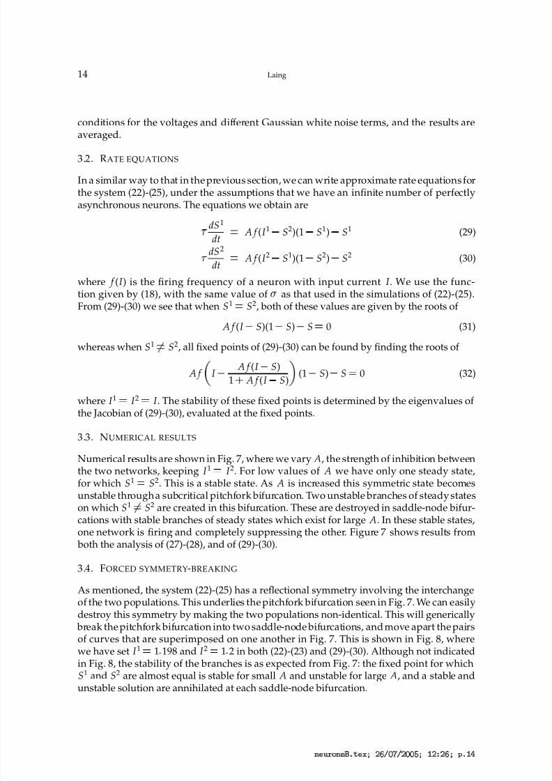
Numerical results are shown in Fig. 7, where we vary A, the strength of inhibition betweenthe two networks, keeping I 1 I 2. For low values of A we have only one steady state,for which S1 S2. This is a stable state. As A is increased this symmetric state becomesunstable through a subcritical pitchfork bifurcation. Two unstable branches of steady stateson which S1 ¤
S2 are created in this bifurcation. These are destroyed in saddle-node bifur-cations with stable branches of steady states which exist for large A. In these stable states,one network is firing and completely suppressing the other. Figure 7 shows results from
both the analysis of (27)-(28), and of (29)-(30).
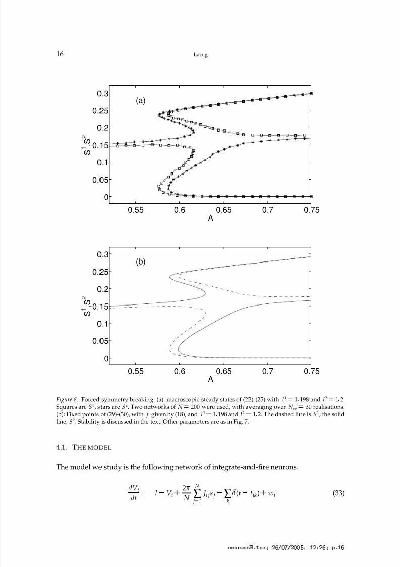
3.4. FORCED SYMMETRY-BREAKING
As mentioned, the system (22)-(25) has a reflectional symmetry involving the interchangeof the two populations. This underlies the pitchfork bifurcation seen in Fig. 7. We can easilydestroy this symmetry by making the two populations non-identical. This will generically
break the pitchfork bifurcation into two saddle-node bifurcations, and move apart the pairsof curves that are superimposed on one another in Fig. 7. This is shown in Fig. 8, wherewe have set I 1 1 198 and I 2 1 2 in both (22)-(23) and (29)-(30). Although not indicatedin Fig. 8, the stability of the branches is as expected from Fig. 7: the fixed point for whichS1 and S2 are almost equal is stable for small A and unstable for large A, and a stable and
unstable solution are annihilated at each saddle-node bifurcation.
3 4 6 8 @ 3 B C D F 4 H P Q S T U V T Q U U X P Y Q a Q S P c D Y ¢
8/3/2019 Carlo R. Laing- On the application of "equation-free" modelling to neural systems
http://slidepdf.com/reader/full/carlo-r-laing-on-the-application-of-equation-free-modelling-to-neural-systems 15/34
Equation-free modelling 15
0.55 0.6 0.65 0.7 0.75
0
0.05
0.1
0.15
0.2
0.25
0.3
A
S 1
, S 2
Figure 7. Steady states for a pair of mutually inhibiting populations. The system is symmetric with respectto interchanging S1 and S2. Circles and crosses joined by lines indicate macroscopic steady states of (22)-(25).Circles indicate stable states and crosses unstable, as determined by the sign of the most positive eigenvaluesof the Jacobian of (27)-(28). Along the “central” branch, S1 ¡ S2, while along the other branches S1
¡ S2. Weused two networks of N ¡ 1000 neurons each, averaging over N av
¡ 50 realisations. Solid lines are stable
fixed points of (29)-(30) while dashed lines are unstable fixed points of these equations. Other parameters areI 1 ¡ I 2 ¡ 1 2
¡ 50 ¡
¡ 0 0245.
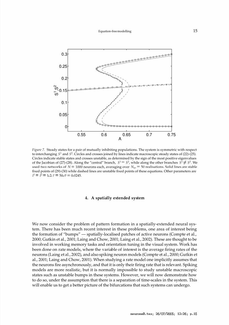
4. A spatially extended system
We now consider the problem of pattern formation in a spatially-extended neural sys-
tem. There has been much recent interest in these problems, one area of interest beingthe formation of “bumps” — spatially-localised patches of active neurons (Compte et al.,2000; Gutkin et al., 2001; Laing and Chow, 2001; Laing et al., 2002). These are thought to beinvolved in working memory tasks and orientation tuning in the visual system. Work has
been done on rate models, where the variable of interest is the average firing rates of theneurons (Laing et al., 2002), and also spiking neuron models (Compte et al., 2000; Gutkin etal., 2001; Laing and Chow, 2001). When studying a rate model one implicitly assumes thatthe neurons fire asynchronously, and that it is only their firing rate that is relevant. Spikingmodels are more realistic, but it is normally impossible to study unstable macroscopicstates such as unstable bumps in these systems. However, we will now demonstrate howto do so, under the assumption that there is a separation of time-scales in the system. This
will enable us to get a better picture of the bifurcations that such systems can undergo.
3 4 6 8 @ 3 B C D F 4 H P Q S T U V T Q U U X P Y Q a Q S P c D Y X
8/3/2019 Carlo R. Laing- On the application of "equation-free" modelling to neural systems
http://slidepdf.com/reader/full/carlo-r-laing-on-the-application-of-equation-free-modelling-to-neural-systems 16/34
16 Laing
0.55 0.6 0.65 0.7 0.750
0.05
0.1
0.15
0.2
0.25
0.3(a)
A
S 1
, S 2
0.55 0.6 0.65 0.7 0.75
0
0.05
0.1
0.15
0.2
0.25
0.3(b)
A
S 1
, S 2
Figure 8. Forced symmetry breaking. (a): macroscopic steady states of (22)-(25) with I 1 ¡ 1 198 and I 2 ¡ 1 2.Squares are S1, stars are S2. Two networks of N ¡ 200 were used, with averaging over N av
¡ 30 realisations.(b): Fixed points of (29)-(30), with f given by (18), and I 1 ¡ 1 198 and I 2 ¡ 1 2. The dashed line is S1; the solidline, S2. Stability is discussed in the text. Other parameters are as in Fig. 7.
4.1. THE MODEL
The model we study is the following network of integrate-and-fire neurons.
dV i
dt
I
V i
¡
2!
N
N
∑ j ¥ 1 J i js j
∑k£
(t
tik)
¡
wi (33)
3 4 6 8 @ 3 B C D F 4 H P Q S T U V T Q U U X P Y Q a Q S P c D Y S
8/3/2019 Carlo R. Laing- On the application of "equation-free" modelling to neural systems
http://slidepdf.com/reader/full/carlo-r-laing-on-the-application-of-equation-free-modelling-to-neural-systems 17/34
Equation-free modelling 17
0 20 40 60
0
0.2
0.4
0.6
0.8
Neuron index, i
s i
0 20 40 60−0.1
0
0.1
0.2
0.3
Neuron index, i
C o u p l i n g f u n c t i o n
J i j
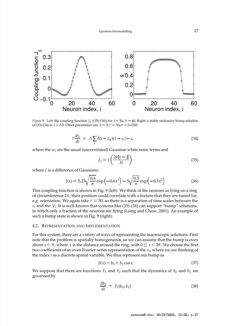
Figure 9. Left: the coupling function J ij ((35)-(36)) for j ¡ 30 N ¡ 60. Right: a stable stationary bump solutionof (33)-(34) at I ¡ 0 9. Other parameters are A ¡ 5
¡ 50 ¡
¡ 0 0245.
¡
dsidt
A∑k
£(t
tik)(1
si)
si (34)
where the wi are the usual (uncorrelated) Gaussian white noise terms and
J i j J ¦
2!
¢
i
j¢
N §
(35)
where J is a difference of Gaussians:
J (x) 5 25
0 6
!
exp$
0 6x2 %
5
0 5
!
exp$
0 5x2 % (36)
This coupling function is shown in Fig. 9 (left). We think of the neurons as lying on a ringof circumference 2
!
; their position could correlate with a feature that they are tuned for,e.g. orientation. We again take ¡
50, so there is a separation of time scales between thesi and the V i. It is well-known that systems like (33)-(34) can support “bump” solutions,in which only a fraction of the neurons are firing (Laing and Chow, 2001). An example of such a bump state is shown in Fig. 9 (right).
4.2. REPRESENTATION AND IMPLEMENTATION
For this system, there are a variety of ways of representing the macroscopic solutions. Firstnote that the problem is spatially homogeneous, so we can assume that the bump is evenabout x
!
, where x is the distance around the ring, with 0¡
x£
2!
. We choose the firsttwo coefficients of an even Fourier series representation of the s i, where we are thinking of the index i as a discrete spatial variable. We thus represent our bump as
S(x) b0¡
b1 cos x (37)
We suppose that there are functions F1 and F2 such that the dynamics of b0 and b1 aregoverned by
db0dt
F1(b0 ¦ b1) (38)
3 4 6 8 @ 3 B C D F 4 H P Q S T U V T Q U U X P Y Q a Q S P c D Y V
8/3/2019 Carlo R. Laing- On the application of "equation-free" modelling to neural systems
http://slidepdf.com/reader/full/carlo-r-laing-on-the-application-of-equation-free-modelling-to-neural-systems 18/34
18 Laing
db1
dt
F2(b0 ¦ b1) (39)
and that these can faithfully represent the dynamics of bumps in (33)-(34). See below fordiscussion about our choice of macroscopic variables.
Our restricting operator m takes the values
si¡
and generates b0 and b1 via
b0
1
N
N
∑i
¥ 1
si and b1
2
N
N
∑i
¥ 1
si cos¦
2!
i
N §
(40)
(This is just the first two terms of a discrete cosine transform of the s i.) Our lifting operator M generates initial conditions
si(0)¡
from b0 and b1 in the obvious way:
si(0)
b0¡
b1 cos ¦
2!
i
N § i
1 ¦
¦ N (41)
For simplicity we do not include any random components in the
si(0)¡
, although it would be consistent to add a random number from a distribution with mean zero to each s i(0),for example.
The initial conditions for the V i are generated in a similar way to that in earlier sections.Given the set
si(0)¡
, for each neuron we calculate the initial effective drive current:
I i I
¡
2!
N
N
∑ j
¥ 1
J i js j(0) i 1¦
¦ N (42)
We then choose each V i(0) from the PDF p(V i(0)
¢
I i), where p is given by (10).We estimate F1(b0(0)
¦b1(0)) and F2(b0(0)
¦b1(0)) in the usual way. Given values of b0(0)
and b1(0), lift them to initial conditions using eqn. (41) and generate the V i(0) as above, runthe system (33)-(34) for 20 time steps, generating b0(t) and b1(t) using the time-dependentversions of (40), then do a least-squares fit to find the slopes of b0(t) and b1(t) as func-tions of time over the time interval [10
¦
20]. These are our estimates of F1(b0(0)¦b1(0)) and
F2(b0(0)¦b1(0)), respectively. Actually, N av simulations are run in parallel, with different
initial conditions for the V i and different realisations of the white noise, and the s i(t) arethen averaged over realisations before b0(t) and b1(t) are generated and the slopes are fit.Another possibility would be to find the slopes for each realisation, and then average theseslopes.
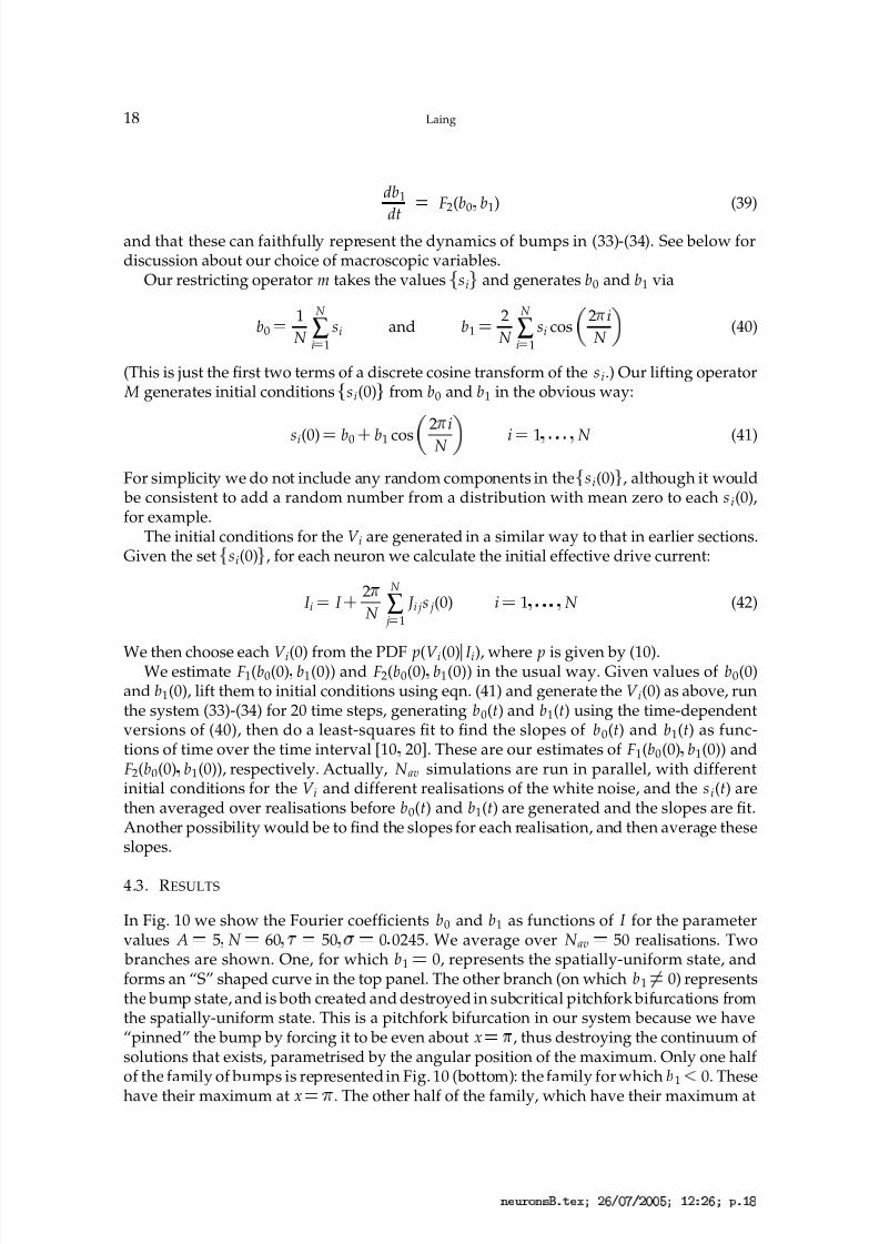
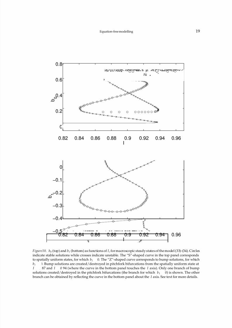
4.3. RESULTS
In Fig. 10 we show the Fourier coefficients b0 and b1 as functions of I for the parametervalues A 5
¦N 60
¦
¡
50¦
¤ 0 0245. We average over N av 50 realisations. Two
branches are shown. One, for which b1 0, represents the spatially-uniform state, and
forms an “S” shaped curve in the top panel. The other branch (on which b1¤ 0) represents
the bump state, and is both created and destroyed in subcritical pitchfork bifurcations fromthe spatially-uniform state. This is a pitchfork bifurcation in our system because we have“pinned” the bump by forcing it to be even about x
!
, thus destroying the continuum of solutions that exists, parametrised by the angular position of the maximum. Only one half of the family of bumps is represented in Fig. 10 (bottom): the family for which b1 £
0. These
have their maximum at x
! . The other half of the family, which have their maximum at
3 4 6 8 @ 3 B C D F 4 H P Q S T U V T Q U U X P Y Q a Q S P c D Y £
8/3/2019 Carlo R. Laing- On the application of "equation-free" modelling to neural systems
http://slidepdf.com/reader/full/carlo-r-laing-on-the-application-of-equation-free-modelling-to-neural-systems 19/34
Equation-free modelling 19
0.82 0.84 0.86 0.88 0.9 0.92 0.94 0.96
0
0.2
0.4
0.6
0.8
I
b 0
0.82 0.84 0.86 0.88 0.9 0.92 0.94 0.96−0.5
−0.4
−0.3
−0.2
−0.1
0
I
b 1
Figure10. b0 (top) and b1 (bottom) as functions of I , for macroscopic steady states of the model (33)-(34). Circlesindicate stable solutions while crosses indicate unstable. The “S”-shaped curve in the top panel correspondsto spatially uniform states, for which b1
¡ 0. The “Z”-shaped curve corresponds to bump solutions, for whichb1
¡ 0. Bump solutions are created/destroyed in pitchfork bifurcations from the spatially uniform state atI 0 87 and I 0 94 (where the curve in the bottom panel touches the I axis). Only one branch of bumpsolutions created/destroyed in the pitchfork bifurcations (the branch for which b1
¡
0) is shown. The other branch can be obtained by reflecting the curve in the bottom panel about the I axis. See text for more details.
3 4 6 8 @ 3 B C D F 4 H P Q S T U V T Q U U X P Y Q a Q S P c D Y
8/3/2019 Carlo R. Laing- On the application of "equation-free" modelling to neural systems
http://slidepdf.com/reader/full/carlo-r-laing-on-the-application-of-equation-free-modelling-to-neural-systems 20/34
20 Laing
x 0 and which have b1 ¢0, can be obtained by reflecting the curve in Fig. 10 (bottom)
about the I axis.Stability is also indicated in Fig. 10. This is determined by examining the eigenvalues
of the 2¨
2 Jacobian of the associated differential equations for b0 and b1, at the steadystates. On the “middle” branch of the spatially-uniform state, both of these eigenvaluesare positive. On all other unstable branches, one eigenvalue is positive and the othernegative. When following the spatially-uniform state through a pitchfork bifurcation, theeigenvector corresponding to the zero eigenvalue has a large entry in the b1 componentand a very small entry in the b0 component, indicating that the instability acts to break thespatial uniformity. Note that there are regions of both bistability and tristability, betweenthe “all-off” state, the bump state, and the “all-on” state.
By tracing out the unstable branches, we have been able to piece together the stable
branches, which are the only branches we would have observed using straight-forwardnumerical integration.
4.4. A RATE MODEL
As with some previous examples, we can derive an effective rate model whose dynamicsshould closely mimic those of the spiking neural network (33)-(34). The sum over j ineqn. (33) is the discretised version of the convolution of J and S, where J is the continu-ous function (36). Thus, moving to a spatial continuum, the effective drive to a neuron atposition x is I
¡
( J S)(x), where the convolution of J and S is given by
( J S)(x)
"
2 ¡
0
J (x
y)S( y) dy (43)
Replacing the sum of delta functions in (34) by the firing rate f , where f is given by (18),we obtain the nonlocal PDE
¡
¢S(x
¦t)
¢t
A f [I ¡
( J S)(x)][1
S(x¦t)]
S(x¦t) (44)
Writing S as the Fourier series (37), we can find the differential equations that b0 and b1
obey:
¡
db0
dt
A(1
b0)
2!
"
2 ¡
0 f ( g(x)) dx
Ab1
2!
"
2 ¡
0 f ( g(x))cos(x) dx
b0 (45)
¡ db1
dt A(1 b0)
!
"
2¡
0 f ( g(x))cos(x) dx
Ab1
!
"
2¡
0 f ( g(x))cos2 (x) dx
b1 (46)
where g(x) I
¡¢
b0¡
¤
b1 cos x (47)
and
¢
"
2 ¡
0 J ( y) dy and
¤
"
2 ¡
0 J ( y)cos y dy (48)
Note that the manifold defined by b1 0 is invariant, and on this manifold the dynamics
of b0 are given by
¡
db0dt
A f (I ¡ ¢
b0) (1 b0) b0 (49)
3 4 6 8 @ 3 B C D F 4 H P Q S T U V T Q U U X P Y Q a Q S P c D Q U
8/3/2019 Carlo R. Laing- On the application of "equation-free" modelling to neural systems
http://slidepdf.com/reader/full/carlo-r-laing-on-the-application-of-equation-free-modelling-to-neural-systems 21/34
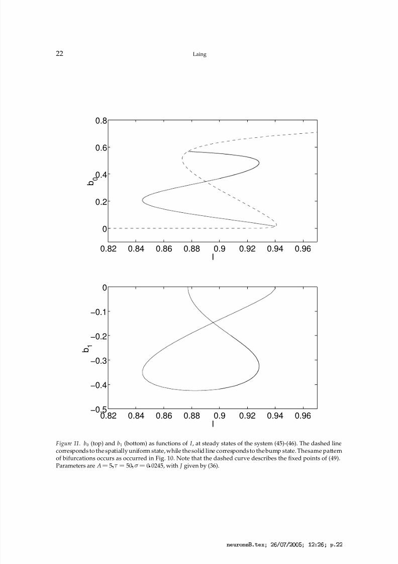
Equation-free modelling 21
Comparing this with eqn. (14), which is derived for a homogeneous population with pos-
itive feedback, we see the similarities, and also the importance of the quantity¢
, equal to2
!
times the mean of J . Fixed points of (49) are shown with a dashed line in Fig. 11 (top).In Fig. 11 we show fixed points of (45)-(46) as I is varied, for both the bump state and
the spatially-uniform state. We see very good agreement with the results obtained fromthe network of spiking neurons (Fig. 10). However, we now discuss a situation in which itis not possible to derive an equivalent rate formulation, for which EF modelling providesinformation that could not be derived any other way.
4.5. INCLUDING GAP JUNCTIONS
Although much of the communication between neurons occurs through synapses, thereare often significant connections via gap junctions (Chow and Kopell, 2000; Kopell and
Ermentrout, 2004). To investigate the effects of including such connections, we modify (33)-(34) to
dV idt
I
V i¡
(V i © 1
2V i¡
V i¡ 1)
¡
2!
N
N
∑ j
¥ 1
J i js j ∑
k
£(t
tik)¡
wi (50)
¡
dsidt
A∑k
£(t
tik)(1
si)
si (51)
where
¢0 is a measure of gap junction conductivity, and V
¡ 1 V N and V N © 1
V 1.All other terms have their previous meanings. Including a term like this acts to keep thevoltages of neighbouring neurons more similar.
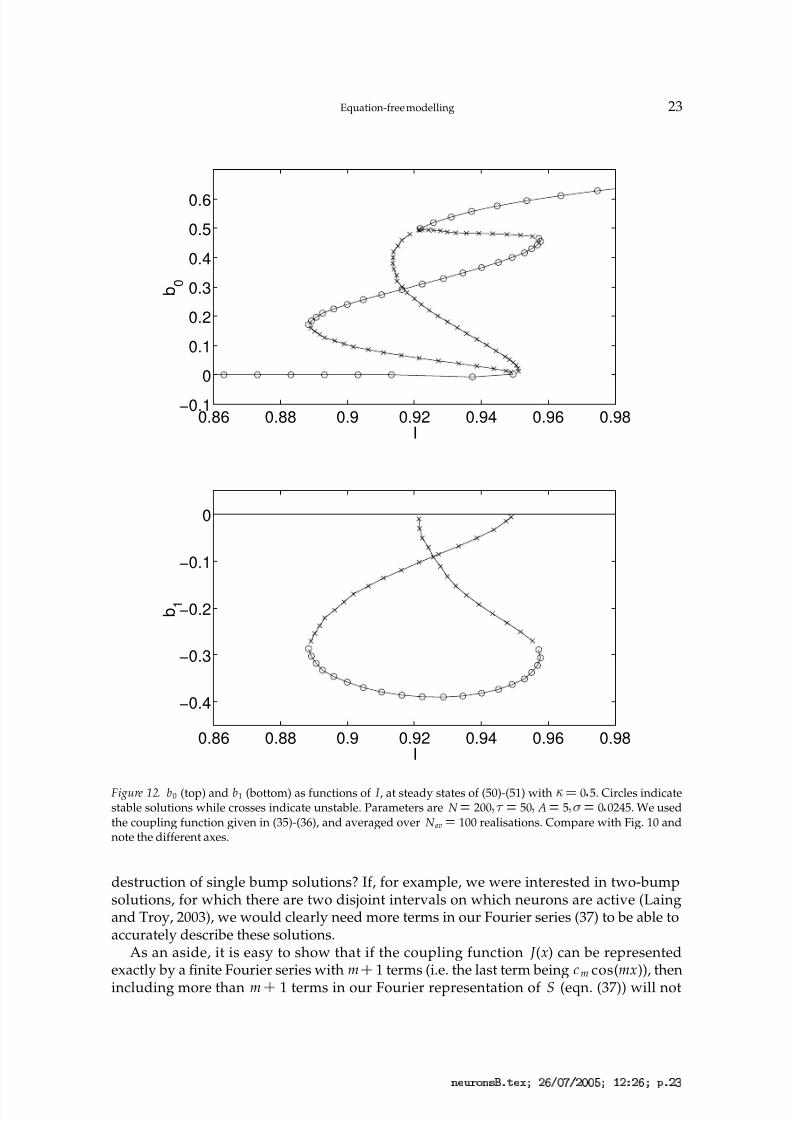
In Fig. 12 we show results of the same form as those in Fig. 10, but for (50)-(51) with
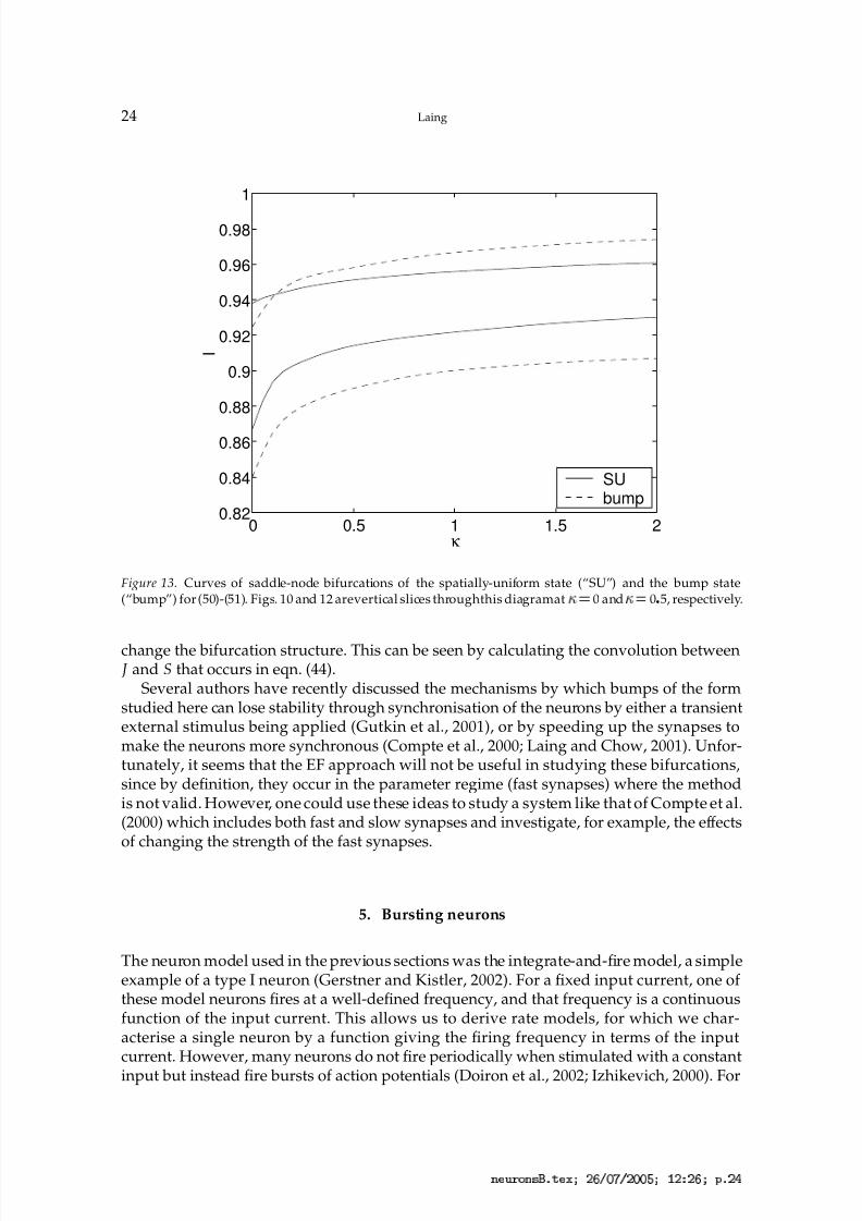
0 5. Including gap junctions in this way simultaneously decreases the size of the interval of I values for which the system can support a stable bump and shifts this interval to highervalues of I . We further demonstrate this in Fig. 13 where we trace the four saddle-node
bifurcations in Figs. 10 and 12 as is varied.The inclusion of the term involving voltage differences in (50) means that deriving a
rate model description of (50)-(51) [such as that in Sec. 4.4 for the system (33)-(34)] is notpossible. Thus, as far as we are aware, these results are novel and could not be derived anyother way. This demonstrates one of the limitations of rate models. Note that from the EFpoint of view, macroscopic stationary states of (50)-(51) are just as easy to analyse as thoseof (33)-(34). Indeed, further levels of complexity could be included and the model neurons
in (33) could be replaced by models that are as realistic as one would like, and the processrepeated.
4.6. DISCUSSION
An obvious question relates to the appropriateness of representing a bump, an example of which is shown in Fig. 9 (right), by just the first two components of a Fourier series. Themain justification for this is that we are specifically interested in bump solutions whichhave only one maximum on the domain. Previous work on models of this type showsthat they can typically support only one bump, and extensive numerical simulation forthe system (33)-(34) suggests that this is also the case here (not shown). This is an exampleof choosing the macroscopic variables (b0 and b1) so that questions of interest can be an-
swered. In this case, the question is: what bifurcations are responsible for the creation and
3 4 6 8 @ 3 B C D F 4 H P Q S T U V T Q U U X P Y Q a Q S P c D Q Y
8/3/2019 Carlo R. Laing- On the application of "equation-free" modelling to neural systems
http://slidepdf.com/reader/full/carlo-r-laing-on-the-application-of-equation-free-modelling-to-neural-systems 22/34
22 Laing
0.82 0.84 0.86 0.88 0.9 0.92 0.94 0.96
0
0.2
0.4
0.6
0.8
I
b 0
0.82 0.84 0.86 0.88 0.9 0.92 0.94 0.96−0.5
−0.4
−0.3
−0.2
−0.1
0
I
b 1
Figure 11. b0 (top) and b1 (bottom) as functions of I , at steady states of the system (45)-(46). The dashed linecorresponds to the spatially uniform state, while the solid line corresponds to the bump state. Thesame patternof bifurcations occurs as occurred in Fig. 10. Note that the dashed curve describes the fixed points of (49).Parameters are A ¡ 5
¡ 50 ¡
¡ 0 0245, with J given by (36).
3 4 6 8 @ 3 B C D F 4 H P Q S T U V T Q U U X P Y Q a Q S P c D Q Q
8/3/2019 Carlo R. Laing- On the application of "equation-free" modelling to neural systems
http://slidepdf.com/reader/full/carlo-r-laing-on-the-application-of-equation-free-modelling-to-neural-systems 23/34
Equation-free modelling 23
0.86 0.88 0.9 0.92 0.94 0.96 0.98−0.1
0
0.1
0.2
0.3
0.4
0.5
0.6
I
b 0
0.86 0.88 0.9 0.92 0.94 0.96 0.98
−0.4
−0.3
−0.2
−0.1
0
I
b 1
Figure 12. b0 (top) and b1 (bottom) as functions of I , at steady states of (50)-(51) with
¡ 0 5. Circles indicatestable solutions while crosses indicate unstable. Parameters are N ¡ 200
¡ 50 A ¡ 5 ¡
¡ 0 0245. We usedthe coupling function given in (35)-(36), and averaged over N av
¡ 100 realisations. Compare with Fig. 10 andnote the different axes.
destruction of single bump solutions? If, for example, we were interested in two-bumpsolutions, for which there are two disjoint intervals on which neurons are active (Laingand Troy, 2003), we would clearly need more terms in our Fourier series (37) to be able toaccurately describe these solutions.
As an aside, it is easy to show that if the coupling function J (x) can be representedexactly by a finite Fourier series with m
¡
1 terms (i.e. the last term being cm cos(mx)), then
including more than m¡
1 terms in our Fourier representation of S (eqn. (37)) will not
3 4 6 8 @ 3 B C D F 4 H P Q S T U V T Q U U X P Y Q a Q S P c D Q
8/3/2019 Carlo R. Laing- On the application of "equation-free" modelling to neural systems
http://slidepdf.com/reader/full/carlo-r-laing-on-the-application-of-equation-free-modelling-to-neural-systems 24/34
24 Laing
0 0.5 1 1.5 20.82
0.84
0.86
0.88
0.9
0.92
0.94
0.96
0.98
1
κ
I
SUbump
Figure 13. Curves of saddle-node bifurcations of the spatially-uniform state (“SU”) and the bump state(“bump”) for (50)-(51). Figs. 10 and 12 arevertical slices throughthis diagramat
¡ 0 and
¡ 0 5, respectively.
change the bifurcation structure. This can be seen by calculating the convolution between J and S that occurs in eqn. (44).
Several authors have recently discussed the mechanisms by which bumps of the formstudied here can lose stability through synchronisation of the neurons by either a transientexternal stimulus being applied (Gutkin et al., 2001), or by speeding up the synapses tomake the neurons more synchronous (Compte et al., 2000; Laing and Chow, 2001). Unfor-tunately, it seems that the EF approach will not be useful in studying these bifurcations,since by definition, they occur in the parameter regime (fast synapses) where the methodis not valid. However, one could use these ideas to study a system like that of Compte et al.(2000) which includes both fast and slow synapses and investigate, for example, the effectsof changing the strength of the fast synapses.
5. Bursting neurons
The neuron model used in the previous sections was the integrate-and-fire model, a simpleexample of a type I neuron (Gerstner and Kistler, 2002). For a fixed input current, one of these model neurons fires at a well-defined frequency, and that frequency is a continuousfunction of the input current. This allows us to derive rate models, for which we char-acterise a single neuron by a function giving the firing frequency in terms of the inputcurrent. However, many neurons do not fire periodically when stimulated with a constant
input but instead fire bursts of action potentials (Doiron et al., 2002; Izhikevich, 2000). For
3 4 6 8 @ 3 B C D F 4 H P Q S T U V T Q U U X P Y Q a Q S P c D Q ¢
8/3/2019 Carlo R. Laing- On the application of "equation-free" modelling to neural systems
http://slidepdf.com/reader/full/carlo-r-laing-on-the-application-of-equation-free-modelling-to-neural-systems 25/34
Equation-free modelling 25
these neurons, such a characterisation is not appropriate, and it may not be possible to
derive a rate-based approximation.In this section we analyse a network of model “ghostbursting” neurons (Doiron et
al., 2002), coupled with slow excitatory synapses. These neurons are found in the elec-trosensory lateral line lobe of the weakly electric fish Apteronotus leptorhynchus and arethought to be involved in electrosensory processing (Doiron et al., 2003). Although thesecells receive input from the outside world via electroreceptors, the majority of their inputis via feedback loops (Berman and Maler, 1999). We have coupled them with synapseshaving a time-constant of 100msec, where the longest time-constant associated with theintrinsic neuron dynamics is 5msec. The equations are given in Appendix A, along with adiscussion of the implementation of initial conditions.
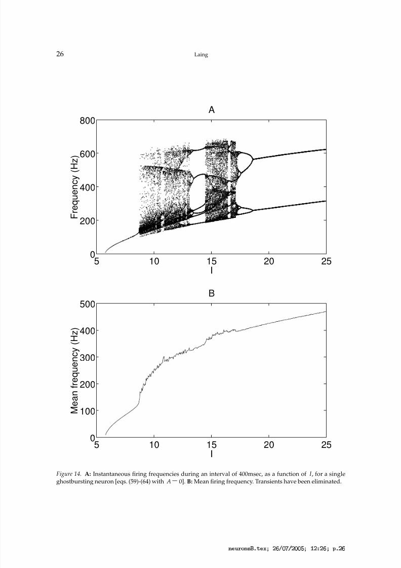
The behaviour of a single isolated ghostbursting neuron [eqs. (59)-(64) with A 0] as
the input current, I , is varied is shown in Fig. 14. The top panel shows the instantaneousfiring frequencies (i.e. reciprocals of the interspike intervals) over a period of 400msec, fordifferent values of I . There are three different types of firing behaviour: (i) periodic firing(5 6
£ I £8 6), (ii) bursting (8 6
£ I £18 6) and (iii) “doublet” firing (18 6
£ I ), in whichthe interspike intervals are alternately short and long (Doiron et al., 2002). Note that thereare many bifurcations as I is varied in the bursting regime. The bottom panel shows theaverage firing frequency as a function of I . The non-smoothness of this curve is due tothe bifurcations that occur as I is varied, and the curve does not become smoother if theaveraging is over more than 400msec (data not shown).
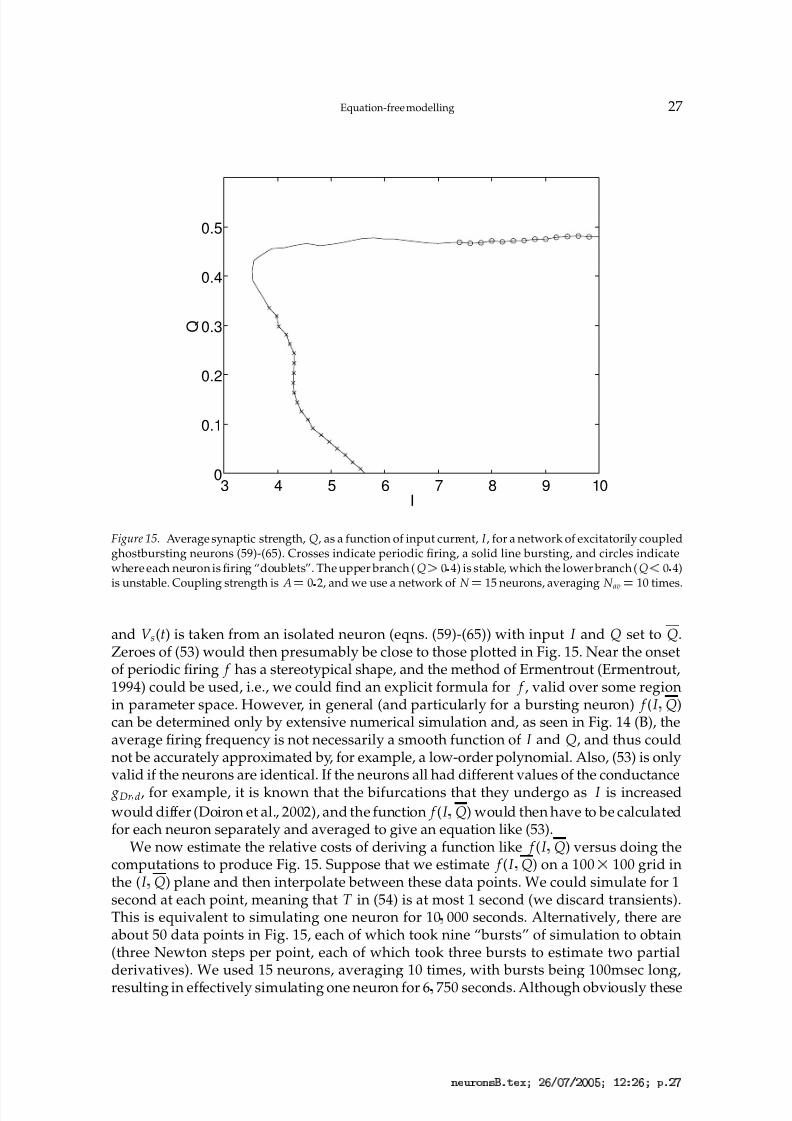
The results for the coupled system [eqs. (59)-(65) with A 0 2] are shown in Fig. 15,where we plot Q, the average synaptic strength, as a function of the input current to theneuron somas (all equal). As expected, the excitatory nature of the coupling causes bistabil-ity to occur, with stable firing now possible at values of I below the threshold for the onsetof firing in an isolated neuron (I '
5 6). (Quiescence is also stable for these values of I .)With reference to Fig. 14, we can divide the curve in Fig. 15 into three sections, dependingon whether the neurons are firing periodically, bursting, or firing doublets. We see that onthe stable branch, the neurons are either bursting or firing doublets, while on the unstable
branch they are either bursting or firing periodically.The curve in Fig. 15 is relatively smooth, in comparison with the curve in Fig. 14 (B), pre-
sumably because coupling the neurons in this all-to-all fashion and measuring an averagequantity “smears out” the fine structure seen in Fig. 14. While knowing the details of thefine structure may be of interest when one is analysing the behaviour of an individualneuron, it could be argued that the behaviour shown in Fig. 15 is a more appropriate
representation of the macroscopic fixed points of the coupled system.To attempt to derive a macroscopic equation governing the behaviour of this system,
one could take the equation for the evolution of the slow variables (65)
100dqi
dt ¤ (V is)(1
qi)
qi (52)
and replace it by
100dQ
dt f (I ¦ Q)(1
Q)
Q (53)
where
f (I ¦ Q)
limT ¢ ¡
1
T "
T
0
¤
(V s(t)) dt (54)
3 4 6 8 @ 3 B C D F 4 H P Q S T U V T Q U U X P Y Q a Q S P c D Q X
8/3/2019 Carlo R. Laing- On the application of "equation-free" modelling to neural systems
http://slidepdf.com/reader/full/carlo-r-laing-on-the-application-of-equation-free-modelling-to-neural-systems 26/34
26 Laing
5 10 15 20 250
200
400
600
800
I
F r e q u
e n c y ( H z )
A
5 10 15 20 250
100
200
300
400
500
I
M e a
n f r e q u e n c y ( H z )
B
Figure 14. A: Instantaneous firing frequencies during an interval of 400msec, as a function of I , for a singleghostbursting neuron [eqs. (59)-(64) with A ¡ 0]. B: Mean firing frequency. Transients have been eliminated.
3 4 6 8 @ 3 B C D F 4 H P Q S T U V T Q U U X P Y Q a Q S P c D Q S
8/3/2019 Carlo R. Laing- On the application of "equation-free" modelling to neural systems
http://slidepdf.com/reader/full/carlo-r-laing-on-the-application-of-equation-free-modelling-to-neural-systems 27/34
Equation-free modelling 27
3 4 5 6 7 8 9 100
0.1
0.2
0.3
0.4
0.5
I
Q
Figure 15. Average synaptic strength, Q, as a function of input current, I , for a network of excitatorily coupledghostbursting neurons (59)-(65). Crosses indicate periodic firing, a solid line bursting, and circles indicatewhere each neuron is firing “doublets”. The upper branch (Q
0 4) is stable, which the lower branch (Q¡
0 4)
is unstable. Coupling strength is A
¡
0 2, and we use a network of N
¡
15 neurons, averaging N av¡
10 times.
and V s(t) is taken from an isolated neuron (eqns. (59)-(65)) with input I and Q set to Q.Zeroes of (53) would then presumably be close to those plotted in Fig. 15. Near the onsetof periodic firing f has a stereotypical shape, and the method of Ermentrout (Ermentrout,1994) could be used, i.e., we could find an explicit formula for f , valid over some regionin parameter space. However, in general (and particularly for a bursting neuron) f (I
¦Q)
can be determined only by extensive numerical simulation and, as seen in Fig. 14 (B), theaverage firing frequency is not necessarily a smooth function of I and Q, and thus couldnot be accurately approximated by, for example, a low-order polynomial. Also, (53) is onlyvalid if the neurons are identical. If the neurons all had different values of the conductance gDr
¡
d, for example, it is known that the bifurcations that they undergo as I is increased
would differ (Doiron et al., 2002), and the function f (I ¦Q) would then have to be calculated
for each neuron separately and averaged to give an equation like (53).We now estimate the relative costs of deriving a function like f (I
¦Q) versus doing the
computations to produce Fig. 15. Suppose that we estimate f (I ¦Q) on a 100
¨
100 grid inthe (I
¦Q) plane and then interpolate between these data points. We could simulate for 1
second at each point, meaning that T in (54) is at most 1 second (we discard transients).This is equivalent to simulating one neuron for 10
¦000 seconds. Alternatively, there are
about 50 data points in Fig. 15, each of which took nine “bursts” of simulation to obtain(three Newton steps per point, each of which took three bursts to estimate two partialderivatives). We used 15 neurons, averaging 10 times, with bursts being 100msec long,
resulting in effectively simulating one neuron for 6 ¦ 750 seconds. Although obviously these
3 4 6 8 @ 3 B C D F 4 H P Q S T U V T Q U U X P Y Q a Q S P c D Q V
8/3/2019 Carlo R. Laing- On the application of "equation-free" modelling to neural systems
http://slidepdf.com/reader/full/carlo-r-laing-on-the-application-of-equation-free-modelling-to-neural-systems 28/34
28 Laing
numbers can be varied and do not represent the total cost they still indicate that for a
system like this, without an analytic f I curve for each neuron, the EF approach cancompete with more traditional methods, particularly if the system is heterogeneous.
In terms of implementation, there is little difference between the network of burstingneurons studied here and the network of integrate-and-fire neurons studied in Sec. 2 — itis only the complexity of the individual neuron model that has changed. Thus this methodcould easily be extended to networks of very detailed model neurons (for example, thoseof Doiron et al. (2001)) with, for example, less-ordered connectivities.
Although this example is not particularly biologically realistic, since in practice thepositive feedback is faster than that modelled here, it does demonstrate that the ideas putforward here can be used with realistic models that incorporate ion channel dynamics,rather than just integrate-and-fire models. It also demonstrates how to initialise the “fast”
variables in the microscopic description when an explicit probability density function forthem is not known (see Appendix).
6. A noisy network
In this section we discuss a network of coupled excitatory and inhibitory neurons thatcould be used to store a single bit of information, i.e. it is bistable for some range of param-eters, as is the network in Sec. 2. We use integrate-and-fire neurons, as in Secs. 2-4, but nowall of the neurons are subject to high levels of noise, in the form of randomly occurringsynaptic events. We include heterogeneity in the excitatory population, and assume thatthe excitatory synapses are slow and inhibitory ones fast. The system can be thought of asdescribing spatially uniform states of previous working memory models (Compte et al.,2000; Gutkin et al., 2001). The high levels of noise and the fact that the inhibitory synapsesare not slow precludes the derivation of a rate equation for this model.
6.1. THE MODEL
We have N e excitatory neurons and N i inhibitory, with coupling both within and betweenpopulations. The equations are
dV
j
edt
I ¡
¤ j
V je¡
gee(Ee
V je )(Se¡ ¤
je (t))¡
gie(Ei
V je )(Si¡ ¤
ji (t))
∑k
£ (t
t jke )(55)
¡
eds
je
dt A∑
k
£(t
t jke )(1
s je)
s je (56)
dV midt
I i
V mi¡
gei(Ee
V mi )(Se¡ ¤ m
e (t))¡
gii(Ei
V mi )(Si¡ ¤ m
i (t)) ∑
n
£
(t
tmni )(57)
¡
idsmidt
A∑n
£(t
tmni )(1
smi )
smi (58)
for j 1¦
¦N e and m 1
¦
N i. The subscripts on the variables and parameters label
their type (excitatory/inhibitory), and the superscripts index them. t jke is the kth firing time
3 4 6 8 @ 3 B C D F 4 H P Q S T U V T Q U U X P Y Q a Q S P c D Q £
8/3/2019 Carlo R. Laing- On the application of "equation-free" modelling to neural systems
http://slidepdf.com/reader/full/carlo-r-laing-on-the-application-of-equation-free-modelling-to-neural-systems 29/34
Equation-free modelling 29
of the jth excitatory neuron, and similarly for tmni . We have
Se
1
N e
N e
∑ j
¥ 1
s je Si
1
N i
N i
∑m
¥ 1
smi
The functions¤
e
i(t) (mimicking randomly occuring excitatory/inhibitory synaptic activ-
ity) are formed from the sum of pulses of the form 0 1e ¡t
2 (t¢
0), whose arrival times arechosen from a Poisson process whose mean rate is 0.2. There are no correlations betweenarrival times for different neurons, nor between random inhibitory and excitatory input.
Reversal potentials are Ee 1 4
¦Ei
0 5. Other parameters are A 0 3¦
¡
e 30
¦
¡
i
1¦
I i
0
9, gee
5¦
gei
2¦
gie
1. We vary gii. The heterogeneity in the excitatory pop-ulation comes from choosing ¤ j
0 1¡
0 2( j
1)¦
(N e
1), i.e. the current offsets forthe excitatory neurons range uniformly from
0 1 to 0.1. We use N e 160 and N i
40,to model the approximate observed ratio of cell types (Compte et al., 2000). Note that theexcitatory synapses are the only slow variables in the network, mimicking, for example,NMDA-type transmission (Compte et al., 2000).
For this model, we assume that the macroscopic description of the system is given by
dSe ¦dt F(Se ¦
I ), in the usual way. To evaluate F(
Se ¦I ), we choose to initialise the V
je (0) and
V mi (0) from the distribution (10) with I 1 1 (the choice of this value of I was arbitrary), we
set s je(0)
Se for each j, and we choose the smi (0) from a uniform distribution between 0 and A. A more accurate lifting operator, M, could be chosen, but the numerical results indicate
that this one is sufficient, and it is easy to implement. This confirms that the initialisationof the fast variables need not be particularly accurate, as their probability distribution isquickly slaved to the dynamics of the slow variables.
6.2. RESULTS AND DISCUSSION
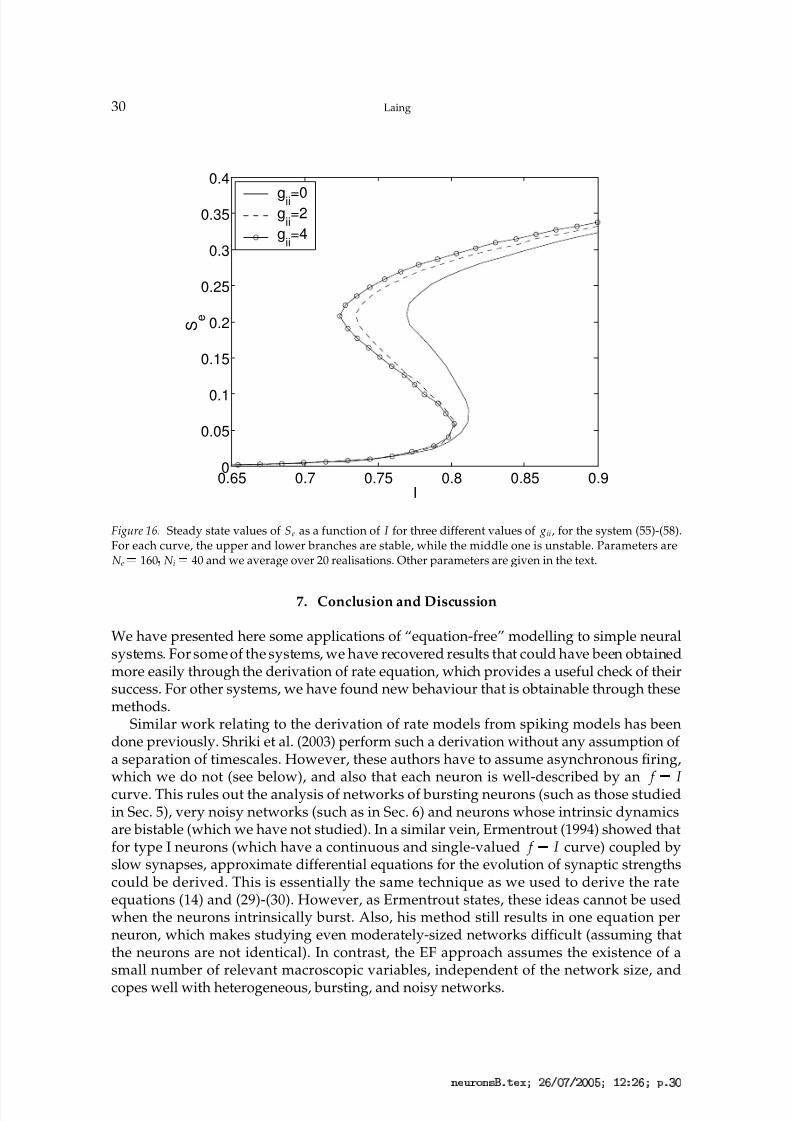
An example of the sort of results we can obtain is shown in Fig. 16, where we plot thesteady state values of Se (the average strength of synaptic connections from the excitatorypopulation) as a function of I (the average current injected into the excitatory population),for three different values of the inhibitory-to-inhibitory conductance ( g
ii). We see that
increasing gii increases the range of values of I for which the system is bistable, for theindicated values of the other parameters. Note that this parameter, g ii, directly affects onlythe dynamics of some of the fast variables, in much the same way that does in the modelin Sec. 4.5. Of course, much more can be determined about this network, in a similar way.
There are several reasons why a rate-based description of this system cannot be analyti-cally derived. One is the high level of noise in the system, in the form of randomly arrivingsynaptic input. This is of such a high intensity and form that it is not meaningful to derivea firing rate function for an uncoupled individual neuron such that given in (18) (which isappropriate only when the noise appears as Gaussian white noise). Another reason is thatwhile the excitatory synapses are slow the inhibitory ones are not. Thus it is not possibleto treat Si as approximately constant, so we cannot derive the firing rate of an individual
neuron as a function of Se and Si, as Ermentrout does (Ermentrout, 1994).
3 4 6 8 @ 3 B C D F 4 H P Q S T U V T Q U U X P Y Q a Q S P c D Q
8/3/2019 Carlo R. Laing- On the application of "equation-free" modelling to neural systems
http://slidepdf.com/reader/full/carlo-r-laing-on-the-application-of-equation-free-modelling-to-neural-systems 30/34
30 Laing
0.65 0.7 0.75 0.8 0.85 0.90
0.05
0.1
0.15
0.2
0.25
0.3
0.35
0.4
I
S e
gii=0g
ii=2
gii=4
Figure 16. Steady state values of Se as a function of I for three different values of gii, for the system (55)-(58).For each curve, the upper and lower branches are stable, while the middle one is unstable. Parameters areN e
¡ 160 N i¡ 40 and we average over 20 realisations. Other parameters are given in the text.
7. Conclusion and Discussion
We have presented here some applications of “equation-free” modelling to simple neuralsystems. For some of the systems, we have recovered results that could have been obtainedmore easily through the derivation of rate equation, which provides a useful check of theirsuccess. For other systems, we have found new behaviour that is obtainable through thesemethods.
Similar work relating to the derivation of rate models from spiking models has beendone previously. Shriki et al. (2003) perform such a derivation without any assumption of a separation of timescales. However, these authors have to assume asynchronous firing,which we do not (see below), and also that each neuron is well-described by an f
I curve. This rules out the analysis of networks of bursting neurons (such as those studiedin Sec. 5), very noisy networks (such as in Sec. 6) and neurons whose intrinsic dynamicsare bistable (which we have not studied). In a similar vein, Ermentrout (1994) showed thatfor type I neurons (which have a continuous and single-valued f
I curve) coupled byslow synapses, approximate differential equations for the evolution of synaptic strengthscould be derived. This is essentially the same technique as we used to derive the rateequations (14) and (29)-(30). However, as Ermentrout states, these ideas cannot be usedwhen the neurons intrinsically burst. Also, his method still results in one equation perneuron, which makes studying even moderately-sized networks difficult (assuming thatthe neurons are not identical). In contrast, the EF approach assumes the existence of asmall number of relevant macroscopic variables, independent of the network size, and
copes well with heterogeneous, bursting, and noisy networks.
3 4 6 8 @ 3 B C D F 4 H P Q S T U V T Q U U X P Y Q a Q S P c D U
8/3/2019 Carlo R. Laing- On the application of "equation-free" modelling to neural systems
http://slidepdf.com/reader/full/carlo-r-laing-on-the-application-of-equation-free-modelling-to-neural-systems 31/34
Equation-free modelling 31
A crucial requirement for the success of EF methods is the separation of time-scales
(although see the remark in Sec. 2.5). Without this, by the time the fast variables have become “slaved” (i.e. after the time
£in Fig. 1) the slow variable(s) will have also changed
significantly, so that a linear approximation to their time derivative will no longer bevalid, and the method is no longer successful. We have only considered slow synapses,
but one hallmark of neural systems is their wide range of time-scales, from the submil-lisecond opening of ion channels to synaptic plasticity that may occur over seconds orlonger (Varela et al., 1997), and the ideas presented here should be more widely applicablethan just to slow synapses. At a more technical level, for the EF approach to work onemust assume that there is a low-dimensional macroscopic description of the state of thesystem which is complete in the sense that the dynamics of the variables in this descriptiondepend only on the values of those variables, i.e. the system is closed (Makeev et al., 2002).
In practice this is difficult, if not impossible, to show, but the usefulness of this methodlies in the results that can be obtained simply by applying the methods, without too muchconcern for their justification.
One issue we have not addressed is the analysis of periodic orbits. The ideas presentedhere can be used to follow both stable and unstable periodic orbits in the phase space of the macroscopic variables (and detect their bifurcations) by treating them as fixed pointsof a return map on a Poincare section. However, one must now consider the relationship
between the period of the periodic orbit and the intrinsic time-scales of the underlyingsystem. For example, it may be necessary to “lift-evolve-restrict” the macroscopic variablesseveral times in succession in order to complete one period of oscillation (Makeev et al.,2002).
Anotherissue not addressed here is synchronisation (although see the remark in Sec. 2.5).It is well known that populations of coupled model neurons can synchronise, and suchsynchronisation is often thought to be important (Gerstner and Kistler, 2002). In the workdiscussed here we have always assumed that the populations of neurons were not synchro-nised, by choosing microscopic initial conditions for each neuron from probability densityfunctions of isolated neurons. This, combined with short simulation times and the additionof noise, ensured that our simulations accurately described states of asynchronous firing.(In the bump states discussed in Sec. 4, synchronous firing is not possible (Laing and Chow,2001).) However, we can still use the ideas presented here even if neurons become synchro-nised at the spike-to-spike level. In this case, we effectively have a population of N 1neuron. As discussed at the end of Sec. 2, this just means that we need to increase N av inorder to obtain accurate estimates of the derivatives of the slow variable(s). Conceptually,
we can see that since our macroscopic variables change on a slow time-scale relative tointerspike intervals, whether neurons are synchronised or not on a spike-to-spike levelwill not affect the rate of change of those variables.
Although we have largely studied stochastic systems here, this is not a requirement forthe EF method to work, as is demonstrated in Sec. 5 where we study a small network of deterministic bursting neurons. Adding noise to the neuron models brings them closer toreality (Koch, 1999), and has the added advantage of smoothing out some of the functionsthat determine the curves of fixed points, making the numerical work easier.
The ideas presented here have also been applied to continuum models with hetero-geneous domains (Runborg et al., 2002), and it would be interesting to apply them toneural field models of the form (44) with, for example, a periodic spatial modulation of the
current, I . Bressloff has studied a similar situation in the context of travelling waves, using
3 4 6 8 @ 3 B C D F 4 H P Q S T U V T Q U U X P Y Q a Q S P c D Y
8/3/2019 Carlo R. Laing- On the application of "equation-free" modelling to neural systems
http://slidepdf.com/reader/full/carlo-r-laing-on-the-application-of-equation-free-modelling-to-neural-systems 32/34
32 Laing
homogenization and averaging (Bressloff, 2001), and it would be interesting to compare
the results of the two different approaches. Another area of interest would be to studya spatially-extended system that is explicitly discrete (i.e. not resulting from discretiz-ing a continuous system) from the point of view of there being an effective continuumdescription of, for example, travelling waves (Moller et al., 2005).
There is nothing in this type of analysis that restricts the model neurons to be identical— indeed, the excitatory population in Sec. 6 is heterogeneous — or even of the same typeor described at the same level of complexity. In principle, neurons in different populationscould be described with different levels of complexity. For example, excitatory neuronscould be modelled using the Hodgkin-Huxley-type formalism, while inhibitory neuronscould be of a more generic nature, e.g. integrate-and-fire.
In summary, we have demonstrated for several neural models a new technique for the
analysis of systems for which a microscopic description is available but for which macro-scopic equations cannot or have not been derived. Many of the results presented here couldhave been derived by using a rate model description with much less computational effort.Specifically, the results derived using EF modelling in Secs. 2,3 and some of Sec. 4 werewell-approximated by results derived from a rate description. However, new results have
been found (in Sec. 4.5 where we investigate the effects of including gap junctions in amodel for “bump” formation, in Sec. 5 describing the coupled ghostbursters, and in Sec. 6,where we study a noisy network with fast inhibitory synapses). We believe that the ideaspresented here are widely applicable and will be valuable in bridging the gap betweendetailed models of single neurons and a macroscopic “coarse” description of the dynamicsof networks of them.
Acknowledgements: I thank Alona Ben-Tal for carefully reading the manuscript, and thereferees for their useful comments. This work was supported by the Marsden Fund ad-ministered by the Royal Society of New Zealand.
Appendix
A. Ghostbursting neuron model
We now give the equations for the network of “ghostbursting” model neurons discussed
in Sec. 5. The single neuron model we use has been presented and analysed elsewhere (Do-iron et al., 2002). For a network of N all-to-all excitatorily coupled neurons the equationsare
CdV isdt
I ¡
gNa¡
sm2¡
¡
s(V is)(1
nis)(V Na
V is)¡
gDr¡
s(nis)
2(V K
V is)
¡
gc(V id
V is) ¦
¡
gleak(V l
V is) (59)
¡
n¡
sdni
s
dt n ¡
¡
s(V is)
nis (60)
CdV iddt
AQ(V id
V e)¡
gNa¡
dm2¡
¡
d(V id)hid(V Na
V id)
¡
gDr¡
d(nid)2 pi
d(V K
V id)¡
gc(V is
V id) ¦ (1
)¡
gleak(V l
V id) (61)
3 4 6 8 @ 3 B C D F 4 H P Q S T U V T Q U U X P Y Q a Q S P c D Q
8/3/2019 Carlo R. Laing- On the application of "equation-free" modelling to neural systems
http://slidepdf.com/reader/full/carlo-r-laing-on-the-application-of-equation-free-modelling-to-neural-systems 33/34
Equation-free modelling 33
¡
h¡
d
dhid
dt
h ¡
¡
d
(V i
d
)
hi
d
(62)
¡
n¡
d
dnid
dt n ¡
¡
d(V id)
nid (63)
¡
p¡
d
dp id
dt p ¡
¡
d(V id)
pid (64)
100dqi
dt ¤ (V is)(1
qi)
qi (65)
for i 1¦
N , where a subscript “s/d” denotes a somatic/dendritic variable, the super-script labels the neuron, and
Q
1
N
N
∑i
¥ 1
qi (66)
Parameters are gNa¡
s 55
¦ gDr¡
s 20
¦ gc 1
¦ gleak 0 18
¦ gNa¡
d 5
¦ gDr¡
d 15, (in units of
mS/cm2) ¡
n¡
s 0 39
¦
¡
h¡
d 1
¦
¡
n¡
d 0 9
¦
¡
p¡
d 5 (in units of msec), V Na
40 mV, V K
88 5 mV, V l
70 mV, V e 0 mV, C 1
¢
F/cm2. The feedback strength A is specified inthe text.
Functions are
m ¡
¡
s(V )
1¡
exp[
(V ¡
40)¦
3]¡
¡ 1 (67)
n ¡
¡
s(V )
1¡
exp[
(V ¡
40)¦
3]¡
¡ 1 (68)
m ¡
¡
d(V )
1¡
exp[
(V ¡
40)¦
5]¡
¡ 1 (69)
h¡
¡ d(V )
1¡
exp[(V ¡
52) ¦ 5] ¡
¡
1 (70)n ¡
¡
d(V )
1¡
exp[
(V ¡
40)¦
5]¡
¡ 1 (71)
p ¡
¡
d(V )
1¡
exp[(V ¡
65)¦
6]¡
¡ 1 (72)¤ (V ) 5
¦
1¡
exp[
(V ¡
20)¦
5]¡
(73)
The macroscopic variable is Q. To implement the microscopic initial conditions, wechose qi(0) Q(0) for i 1
¦
N . To choose the initial conditions for the other variables,we first ran a simulation of an isolated neuron for 70,000 time steps, during which I waslinearly increased from I 7 75 to I 18 25, thus sweeping through a range of possiblestates in which a neuron could be. To initialise N neurons we randomly choose N integersfrom a uniform distribution on [1
¦70
¦000], say k1 ¦
kN . The six initial variables of theith neuron, V is(0)
¦ nis(0)
¦
¦ pid(0) are then set to the state that the “test” neuron was in
at the kith timestep of the sweep. The integers k1 ¦
kN are rechosen at the start of eachsimulation. In this way we hope to initialise each neuron “close” to a state consistent withthe current value of Q.
References
Berman NJ, Maler L (1999) Neural architecture of the electrosensory lateral line lobe: adaptations for co-incidence detection, a sensory searchlight and frequency-dependent adaptive filtering. J. Exp. Biol. 202:1243-1253.
Bressloff PC (2001) Traveling fronts and wave propagation failure in an inhomogeneous neural network.Physica D 155: 83-100.
3 4 6 8 @ 3 B C D F 4 H P Q S T U V T Q U U X P Y Q a Q S P c D
8/3/2019 Carlo R. Laing- On the application of "equation-free" modelling to neural systems
http://slidepdf.com/reader/full/carlo-r-laing-on-the-application-of-equation-free-modelling-to-neural-systems 34/34
34 Laing
Brunel N, Hakim V (1999) Fast global oscillations in networks of integrate-and-fire neurons with low firing
rates. Neural Comput. 11: 1621-1671.Chow CC, Kopell N (2000) Dynamics of spiking neurons with electrical coupling. Neural Comput. 12: 1643-1678.
Compte A, Brunel N, Goldman-Rakic PS, Wang X-J (2000) Synaptic mechanisms and network dynamicsunderlying spatial working memory in a cortical network model. Cereb Cortex 10: 910-923.
DoedelE, KellerHB, Kernevez JP (1991) Numerical analysis and control of bifurcation problems. (I) Bifurcationin finite dimensions. Int. J. Bifn. Chaos. 1: 493-520.
Doiron B, Chacron MJ, Maler L, Longtin A, Bastian J (2003) Inhibitory feedback required for networkoscillatory responses to communication but not prey stimuli. Nature. 421: 539-543.
Doiron B, Laing CR, Longtin A, Maler L (2002) Ghostbursting: a novel neuronal burst mechanism. J. Comput.Neurosci. 12: 5-25.
Doiron B, Longtin A, Turner RW, Maler L (2001) Model of gamma frequency burst discharge generated byconditional backpropagation. J. Neurophysiol. 86: 1523-1545.
Ermentrout B (1994) Reduction of conductance-based models with slow synapses to neural nets. NeuralComput. 6: 679-695.
Fourcaud N, Brunel N (2002) Dynamics of the firing probability of noisy integrate-and-fire neurons. NeuralComput. 14: 2057-2110.
Garcia-Archilla B, Novo J, Titi, ES (1998) Postprocessing the Galerkin method: a novel approach to approxi-mate inertial manifolds. SIAM J. Numer. Anal. 35: 941-972.
Gear CW, Kevrekidis IG, Theodoropoulos C (2002) “Coarse” integration/bifurcation analysis via microscopicsimulators: micro-Galerkin methods. Comp. Chem. Eng. 26: 941-963.
Gerstner W, Kistler W (2002) Spiking neuron models: single neurons, populations, plasticity. CambridgeUniversity Press.
Givon D, Kupferman R, Stuart A (2004) Extracting macroscopic dynamics: model problems and algorithms.Nonlinearity 17: R55-R127.
Gutkin BS, Laing CR, Colby CL, Chow CC, Ermentrout GB (2001). Turning on and off with excitation: the roleof spike-timing asynchrony and synchrony in sustained neural activity. J. Comput. Neurosci. 11: 121-134.
Izhikevich EM (2000) Neural excitability, spiking and bursting. Int. J. Bifn. Chaos. 10: 1171-1266.Kevrekidis IG, Gear CW, Hyman JM, Kevrekidis PG, Runborg O, Theodoropoulos C (2003) Equation-free,
coarse-grained multiscale computation: enabling microscopic simulators to perform system-level analysis.Comm. Math. Sci. 1: 715-762.
Koch C (1999) Biophysics of Computation: Information Processing in Single Neurons. OxfordUniversity Press.Kopell N, Ermentrout B (2004) Chemical and electrical synapses perform complementary roles in the
synchronization of interneuronal networks. Proc. Nat. Acad. Sci. USA 101: 15482-15487.Laing CR, Chow CC (2001) Stationary bumps in networks of spiking neurons. Neural Comput. 13: 1473-1494.Laing CR, Longtin A (2003) Dynamics of deterministic and stochastic paired excitatory-inhibitory delayed
feedback. Neural Comput. 15: 2779-2822.Laing CR, Troy, WC (2003) Two-bump solutions of Amari-type models of neuronal pattern formation.
Physica D 187: 190-218.Laing CR, Troy WC, Gutkin B, Ermentrout GB (2002) Multiple bumps in a neuronal model of working memory.
SIAM J. Appl. Math. 63: 62-97.Makeev AG, Maroudas D, Kevrekedis IG (2002) “Coarse” stability and bifurcation analysis using stochastic
simulators: Kinetic Monte Carlo examples. J. Chem. Phys. 116: 10083-10091.Moller J, Runborg O, Kevrekidis PG, Lust K, Kevrekidis IG (2005) Equation-free, effective computation for
discrete systems: a time stepper based approach. Int. J. Bifn. Chaos. 15: 975-996.Runborg O, Theodoropoulos C, Kevrekidis IG (2002) Effective bifurcation analysis: a time-stepper-based
approach. Nonlinearity. 15: 491-511.Shriki O, Hansel D, Sompolinsky H (2003) Rate models for conductance-based cortical neuronal networks.
Neural Comput. 15: 1809-1841.Varela JA, Sen K, Gibson J, Fost J, Abbott LF, Nelson SB (1997) A quantitative description of short-term
plasticity at excitatory synapses in layer 2/3 of rat primary visual cortex. J. Neurosci. 17: 7926-7940.


![Laing Heating Circulator Ecocirc Vario[1]](https://img.pdfslide.us/doc/110x75/552675504a7959c3238b46fe/laing-heating-circulator-ecocirc-vario1.jpg)