Embed Size (px)
Citation preview
BC–MIT Number Theory Seminar, September 15, 2015
The sum-of-proper-divisors function
Carl Pomerance, Dartmouth College

As we all know, functions in mathematics
are ubiquitous and indispensable.
But what was the very first function
mathematicians studied?
I would submit as a candidate, the
function s(n) of Pythagoras.
1

The sum-of-proper-divisors function
Let s(n) be the sum of the proper divisors of n:
For example:
s(10) = 1 + 2 + 5 = 8, s(11) = 1,
s(12) = 1 + 2 + 3 + 4 + 6 = 16.
In modern notation: s(n) = σ(n)− n, where σ(n) is the sum of
all of n’s natural divisors.
2

Pythagoras noticed that s(6) = 1 + 2 + 3 = 6
If s(n) = n, we say n is perfect.
And he noticed that
s(220) = 284, s(284) = 220.
If s(n) = m, s(m) = n, and m 6= n, we say n,m are an amicable
pair and that they are amicable numbers.
So 220 and 284 are amicable numbers.
3
Some problems
• Are there infinitely many perfect numbers?, And what canwe say about their distribution?
• Are there infinitely many amicable pairs?, And what can wesay about their distribution?
• What can we say about the s-dynamical system?
• What can we say about the distribution of the fractionss(n)/n?
• What numbers are of the form s(n)?
4
Euclid came up with a formula for perfect numbers 2300 years
ago:
If 2p − 1 is prime, then 2p−1(2p − 1) is perfect.
Euler proved that all even perfect numbers are given by
Euclid’s formula.
What about odd perfect numbers? Well, there are none known.
5
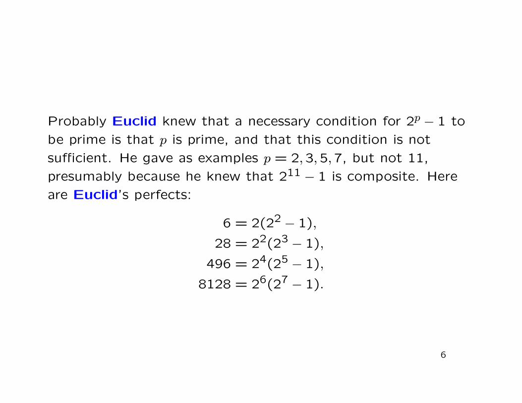
Probably Euclid knew that a necessary condition for 2p − 1 to
be prime is that p is prime, and that this condition is not
sufficient. He gave as examples p = 2,3,5,7, but not 11,
presumably because he knew that 211 − 1 is composite. Here
are Euclid’s perfects:
6 = 2(22 − 1),
28 = 22(23 − 1),
496 = 24(25 − 1),
8128 = 26(27 − 1).
6
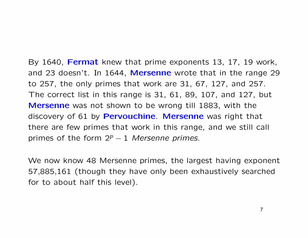
By 1640, Fermat knew that prime exponents 13, 17, 19 work,
and 23 doesn’t. In 1644, Mersenne wrote that in the range 29
to 257, the only primes that work are 31, 67, 127, and 257.
The correct list in this range is 31, 61, 89, 107, and 127, but
Mersenne was not shown to be wrong till 1883, with the
discovery of 61 by Pervouchine. Mersenne was right that
there are few primes that work in this range, and we still call
primes of the form 2p − 1 Mersenne primes.
We now know 48 Mersenne primes, the largest having exponent
57,885,161 (though they have only been exhaustively searched
for to about half this level).
7
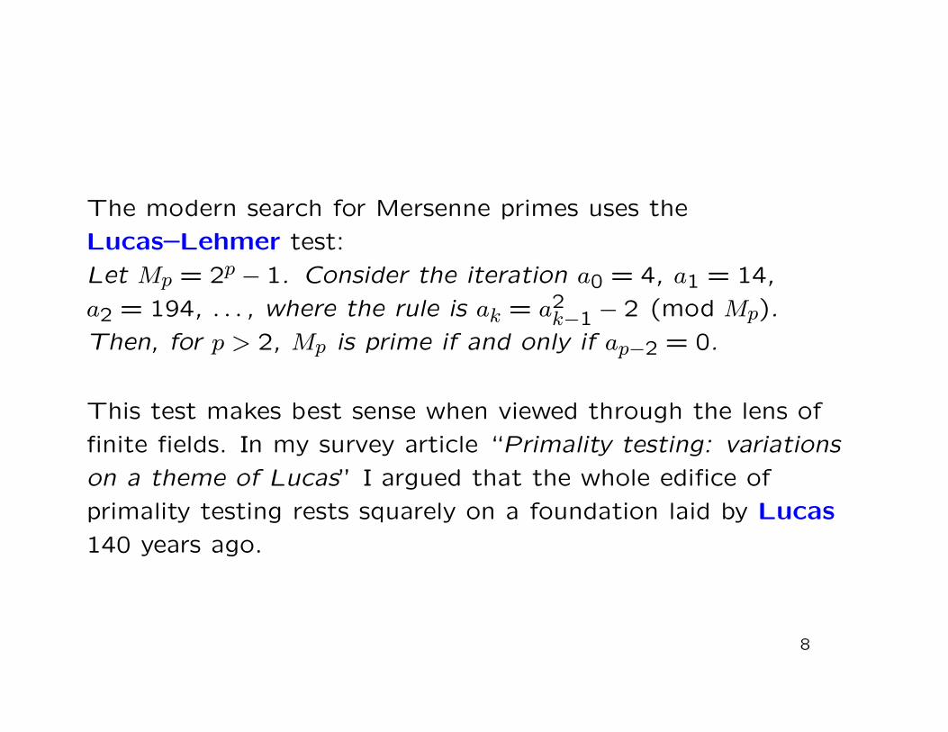
The modern search for Mersenne primes uses the
Lucas–Lehmer test:
Let Mp = 2p − 1. Consider the iteration a0 = 4, a1 = 14,
a2 = 194, . . . , where the rule is ak = a2k−1 − 2 (mod Mp).
Then, for p > 2, Mp is prime if and only if ap−2 = 0.
This test makes best sense when viewed through the lens of
finite fields. In my survey article “Primality testing: variations
on a theme of Lucas” I argued that the whole edifice of
primality testing rests squarely on a foundation laid by Lucas
140 years ago.
8

Probably there are no odd perfect numbers. Here’s why I think
so:
One might view the residue s(n) (mod n) as “random”, where
the event that n is perfect implies s(n) ≡ 0 (mod n). It’s been
known since Euler (and easy to prove) that an odd perfect
number n must be of the form pm2 where p is prime and
p | σ(m2) (= s(m2) +m2). In particular, there are at most
O(logm) possibilities for p, once m is given. Once one of these
p’s is chosen, we will have s(pm2) ≡ 0 (mod p), so there
remains at best a 1/m2 chance that pm2 will be perfect. Since∑(logm)/m2 converges, there should be at most finitely many
odd perfect numbers. But we know there are no small ones, so
it is likely there are none.
9
Let us return to the problem of amicable numbers introduced
by Pythagoras 2500 years ago.
Recall: Two numbers are amicable if the sum of the proper
divisors of one is the other and vice versa. The Pythagoras
example: 220 and 284.
10

In the 9th century, Thabit ibn Qurra found a formula, similar
to Euclid’s for even perfect numbers, that gave a few
examples. Descartes and Fermat rediscovered Thabit’s
formula, and Euler generalized it, finding 58 amicable pairs.
His generalized formula missed the second smallest pair, found
in 1866 by Paganini at the age of 16: namely 1184 and 1210.
So far we know about twelve million pairs, and probably there
are infinitely many, but we have no proof.
11
Beyond individual examples and possible formulas, how are the
amicable numbers distributed within the natural numbers?
Let A(x) denote the number of integers in [1, x] that belong to
an amicable pair. We have no good lower bounds for A(x) as
x→∞, but what about an upper bound?
For perfect numbers, which might be viewed as a subset of the
amicables, we know a fair amount about upper bounds. For
example, the heuristic argument mentioned earlier for odd
perfect numbers can be fashioned into a proof that the number
of perfect numbers to x is O(√x logx).
12
There are much better upper bounds for the distribution of
perfect numbers. The champion result is due to Hornfeck and
Wirsing: the number of perfect numbers in [1, x] is at most
xo(1).
But amicables form a larger set, maybe much larger.
Erdos (1955) was the first to show A(x) = o(x), that is, the
amicable numbers have asymptotic density 0.
His insight: the smaller member of an amicable pair is
abundant (meaning s(n) > n), the larger is deficient (meaning
s(m) < m). Thus, we have an abundant number with the sum
of its proper divisors being deficient.
13
Erdos (1955): A(x) = o(x) as x→∞. Said his method would
give A(x) = O(x/ log log logx).
14
Erdos (1955): A(x) = o(x) as x→∞. Said his method would
give A(x) = O(x/ log log logx).
Rieger (1973): A(x) ≤ x/(log log log logx)1/2, x large.
15
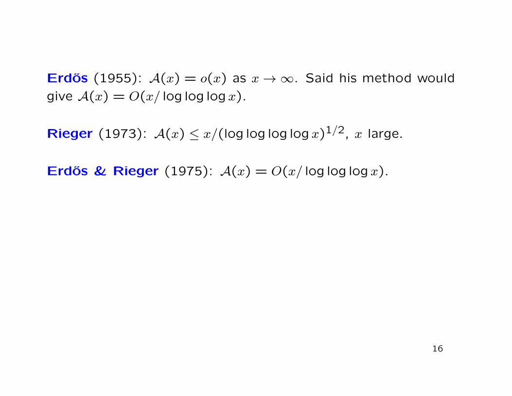
Erdos (1955): A(x) = o(x) as x→∞. Said his method would
give A(x) = O(x/ log log logx).
Rieger (1973): A(x) ≤ x/(log log log logx)1/2, x large.
Erdos & Rieger (1975): A(x) = O(x/ log log logx).
16
Erdos (1955): A(x) = o(x) as x→∞. Said his method would
give A(x) = O(x/ log log logx).
Rieger (1973): A(x) ≤ x/(log log log logx)1/2, x large.
Erdos & Rieger (1975): A(x) = O(x/ log log logx).
P (1977): A(x) ≤ x/ exp((log log logx)1/2), x large.
17
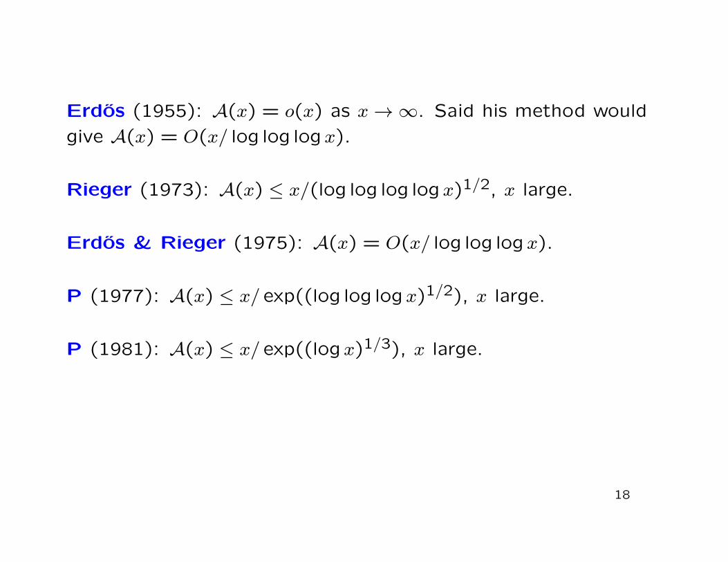
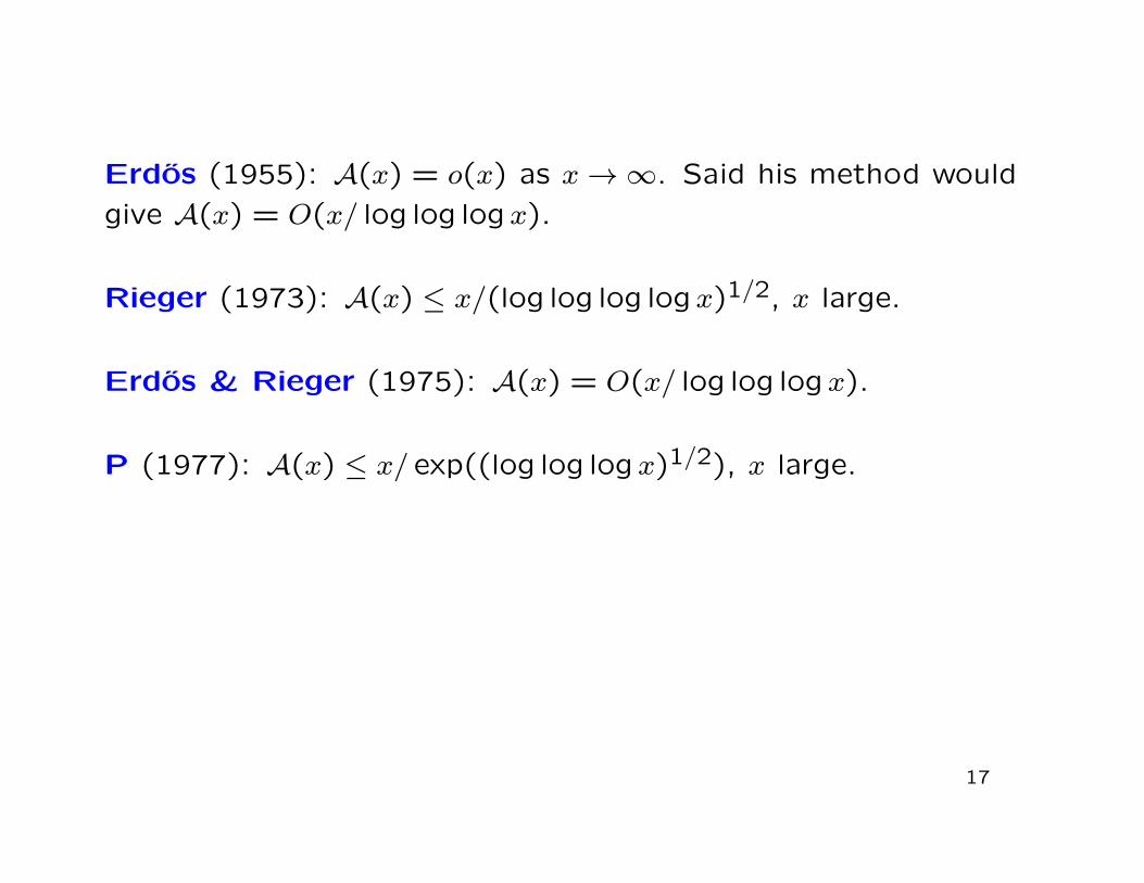
Erdos (1955): A(x) = o(x) as x→∞. Said his method would
give A(x) = O(x/ log log logx).
Rieger (1973): A(x) ≤ x/(log log log logx)1/2, x large.
Erdos & Rieger (1975): A(x) = O(x/ log log logx).
P (1977): A(x) ≤ x/ exp((log log logx)1/2), x large.
P (1981): A(x) ≤ x/ exp((logx)1/3), x large.
18
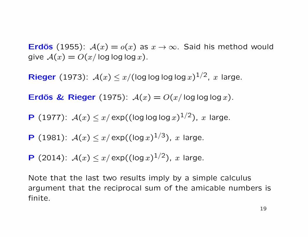
Erdos (1955): A(x) = o(x) as x→∞. Said his method wouldgive A(x) = O(x/ log log logx).
Rieger (1973): A(x) ≤ x/(log log log logx)1/2, x large.
Erdos & Rieger (1975): A(x) = O(x/ log log logx).
P (1977): A(x) ≤ x/ exp((log log logx)1/2), x large.
P (1981): A(x) ≤ x/ exp((logx)1/3), x large.
P (2014): A(x) ≤ x/ exp((logx)1/2), x large.
Note that the last two results imply by a simple calculusargument that the reciprocal sum of the amicable numbers isfinite.
19
So, what is this sum of reciprocals? Using a complete roster of
all amicables to 1014 we can show the reciprocal sum A satisfies
A > 0.0119841556 . . . .
20
So, what is this sum of reciprocals? Using a complete roster of
all amicables to 1014 we can show the reciprocal sum A satisfies
A > 0.0119841556 . . . .
Bayless & Klyve (2011): A < 656,000,000.
21
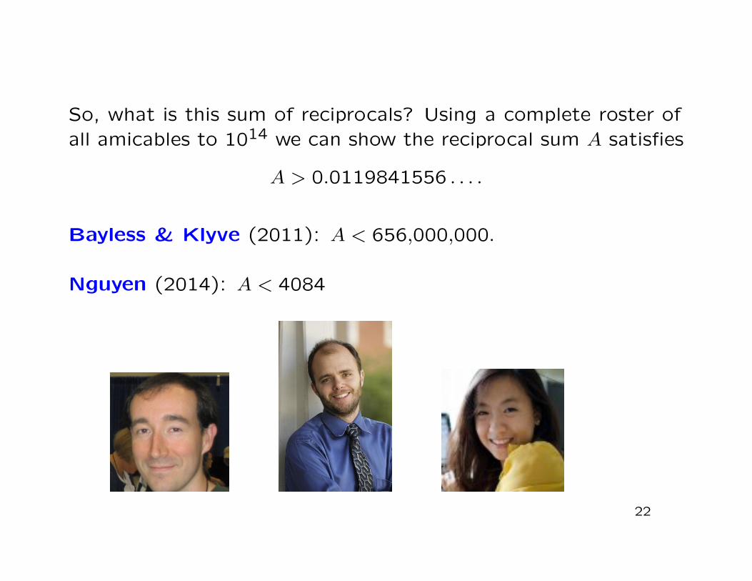
So, what is this sum of reciprocals? Using a complete roster ofall amicables to 1014 we can show the reciprocal sum A satisfies
A > 0.0119841556 . . . .
Bayless & Klyve (2011): A < 656,000,000.
Nguyen (2014): A < 4084
22
Back to Pythagoras:
A number n is perfect if s(n) = n.
A number n is amicable if s(s(n)) = n, but not perfect.
That is, Pythagoras not only invented the first function, but
also the first dynamical system.
Let’s take a look at this system.
Many orbits end at 1, while others cycle:
23
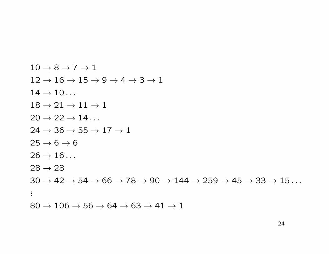
10→ 8→ 7→ 1
12→ 16→ 15→ 9→ 4→ 3→ 1
14→ 10 . . .
18→ 21→ 11→ 1
20→ 22→ 14 . . .
24→ 36→ 55→ 17→ 1
25→ 6→ 6
26→ 16 . . .
28→ 28
30→ 42→ 54→ 66→ 78→ 90→ 144→ 259→ 45→ 33→ 15 . . ....
80→ 106→ 56→ 64→ 63→ 41→ 1
24

Some orbits are likely to be arbitrarily long. For example,
consider the orbit
25→ 6→ 6.
It can be preceded by 95:
95→ 25→ 6→ 6.
And again preceded by 445:
445→ 95→ 25→ 6→ 6.
What’s happening here: To hit an odd number m, write m− 1
as the sum of two different primes: p+ q = m− 1. Then
s(pq) = m. So, Goldbach’s conjecture implies one can back up
forever.
25
Lenstra (1975):
There are arbitrarily long increasing “aliquot” sequences
n < s(n) < s(s(n)) < · · · < sk(n).
Erdos (1976): In fact, for each fixed k, if n < s(n), then
almost surely the sequence continues to increase for k − 1 more
steps.
Nevertheless, we have the Catalan–Dickson conjecture:
Every aliquot sequence is bounded.
Here are some data in graphical form for the sequence starting
with 564. (The least starting number which is in doubt is 276.)
See aliquot.de, maintained by Wolfgang Creyaufmuller.
26
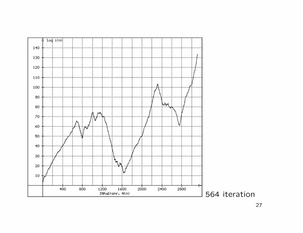
564 iteration27

This has been continued for over 3000 iterations; the numbers
that would need to be factored in order to go farther are over
160 decimal digits.
There are 5 orbits starting below 1000 where it’s not clear
what’s happening:
276, 552, 564, 660, 966,
known as the “Lehmer five”.
The Guy & Selfridge counter conjecture:
For asymptotically all n with n < s(n), the aliquot sequence
starting with n is unbounded.
28

Recently Bosma did a statistical study of
aliquot sequences with starting numbers
below 106. About one-third of the
even starters are still open and running
beyond 1099. Strong evidence for Guy–
Selfridge?
29
One can also ask about cycles in the s-dynamical system
beyond the fixed points (perfect numbers) and 2-cycles
(amicable pairs). There are about 12 million cycles known,
with all but a few being 2-cycles, and most of the rest being
1-cycles and 4-cycles. There are no known 3-cycles, and the
longest known cycle has length 28.
Say a number is sociable if it is in some cycle. Do the sociable
numbers have density 0? The Erdos result on increasing
aliquot sequences shows this if one restricts to cycles of
bounded length. Recently, Kobayashi, Pollack, & P showed
that apart possibly from sociable numbers that are odd and
abundant, they have density 0. Further, we computed that the
density of odd abundant numbers, whether or not they are
sociable, is about 0.002.
30
Earlier we mentioned abundant numbers (s(n) > n) and
deficient numbers (s(n) < n). These terms were defined by
Nicomachus in the 1st century. More generally, one can ask
about
{n : s(n) > un}
for each nonnegative real number u. Does this set have an
asymptotic density? If so, how does it vary as u varies?
The question was first posed for u = 1 by Erich Bessel-Hagen
in 1929.
31
In his 1933 Berlin doctoral thesis, Felix Behrend proved that if
the density exists, it lies between 0.241 and 0.314.
And later in 1933, building on work of I. J. Schoenberg from
1928 dealing with Euler’s function, Harold Davenport showed
the density exists.
In fact, the density D(u) of those n with s(n)/n > u exists, and
D(u) is continuous.
32
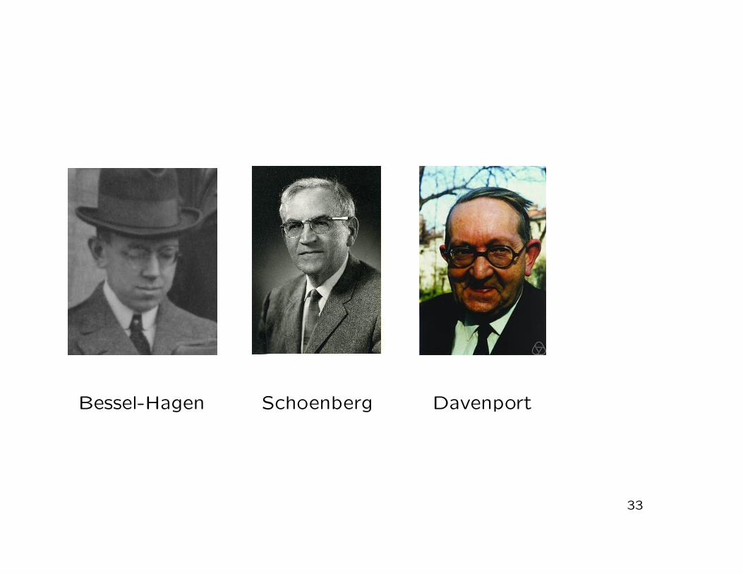
Bessel-Hagen Schoenberg Davenport
33
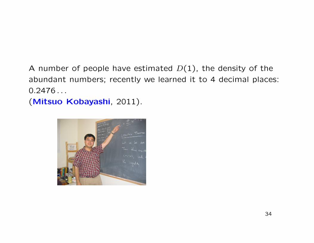
A number of people have estimated D(1), the density of the
abundant numbers; recently we learned it to 4 decimal places:
0.2476 . . .
(Mitsuo Kobayashi, 2011).
34
The Schoenberg–Davenport approach towards the
distribution function of s(n)/n was highly analytic and technical.
Beginning around 1935, Paul Erdos began studying this
subject, looking for the great theorem that would unite and
generalize the work on Euler’s function and s, and also to look
for an elementary method.
This culminated in the Erdos–Wintner theorem in 1939 (with
echoes from Kolmogorov):
35
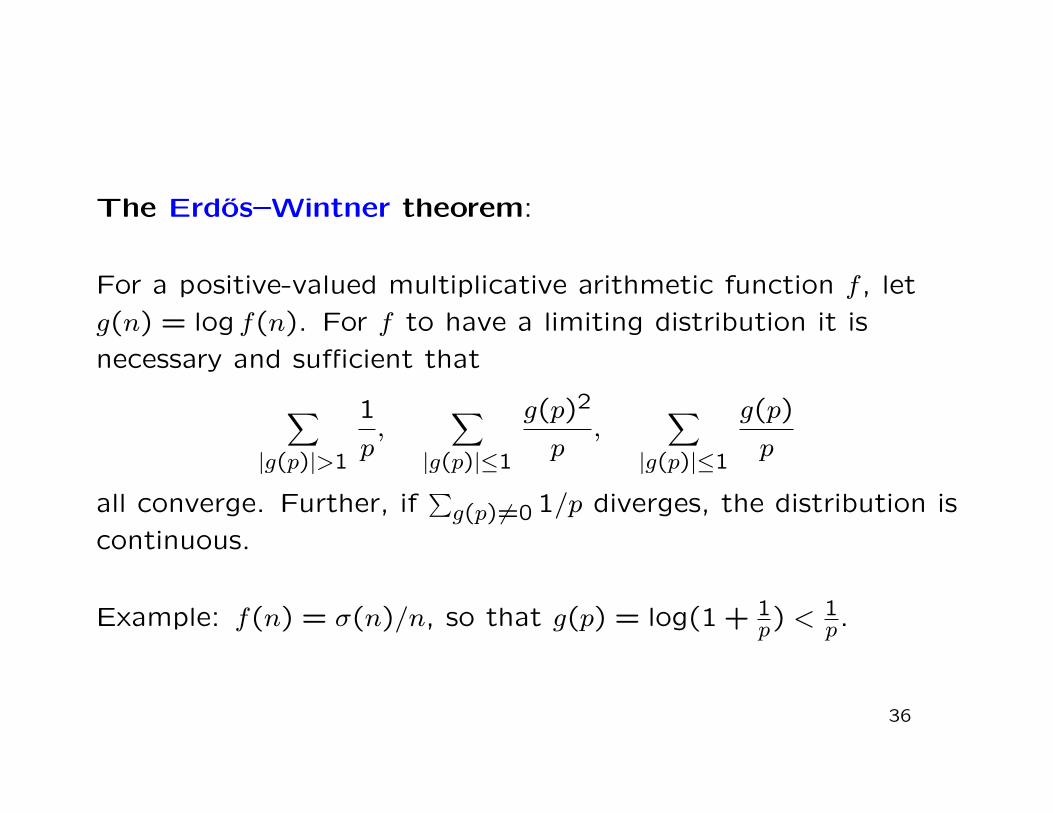
The Erdos–Wintner theorem:
For a positive-valued multiplicative arithmetic function f , let
g(n) = log f(n). For f to have a limiting distribution it is
necessary and sufficient that
∑|g(p)|>1
1
p,
∑|g(p)|≤1
g(p)2
p,
∑|g(p)|≤1
g(p)
p
all converge. Further, if∑g(p) 6=0 1/p diverges, the distribution is
continuous.
Example: f(n) = σ(n)/n, so that g(p) = log(1 + 1p) < 1
p.
36

Erdos Wintner
37
But what of other familiar arithmetic functions such as ω(n),
which counts the number of distinct primes that divide n?
This function is additive, so it is already playing the role of
g(n).
38
However, ω(p) = 1 for all primes p, so the 2nd and 3rd series
diverge.
The solution is in how you measure. Hardy and Ramanujan
had shown that ω(n)/ log logn→ 1 as n→∞ through a set of
asymptotic density 1. There is a threshold function, so one
should be studying the difference ω(n)− log logn.
39
Ramanujan Hardy
40
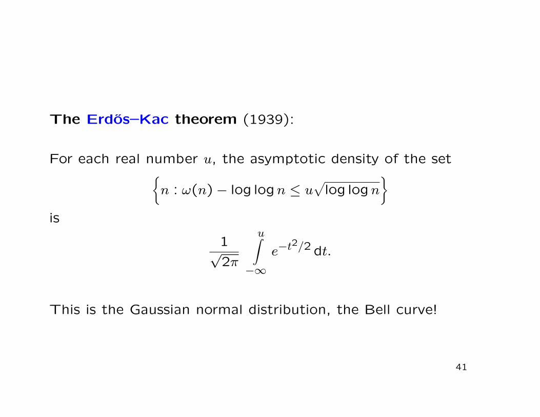
The Erdos–Kac theorem (1939):
For each real number u, the asymptotic density of the set{n : ω(n)− log logn ≤ u
√log logn
}is
1√2π
u∫−∞
e−t2/2 dt.
This is the Gaussian normal distribution, the Bell curve!
41

(!) Kac
42
In 1973, Erdos considered the range of s(n): which integers m
are in the form s(n)? He showed that
• Almost all odd numbers are of the form s(n) (assuming a
slightly stronger form of Goldbach’s conjecture, every odd
number except 5 is in the range).
• There is a positive proportion of even numbers not in the
range.
Last year Luca and P showed that a positive proportion of
even numbers are in the range, and the same goes for any
residue class.
43
This theorem, more likely the proof, may help with the
following.
Erdos, Granville, P, Spiro Conjecture: If A is a set of natural
numbers of positive lower density then s(A) has positive lower
density.
A consequence of this is a conjecture of Erdos: For each k,
but for a set of density 0, if n > s(n), the sequence
n, s(n), s2(n), . . . , sk(n) is decreasing.
As mentioned, Erdos proved the analogous result when
n < s(n).
44
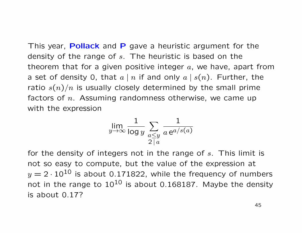
This year, Pollack and P gave a heuristic argument for the
density of the range of s. The heuristic is based on the
theorem that for a given positive integer a, we have, apart from
a set of density 0, that a | n if and only a | s(n). Further, the
ratio s(n)/n is usually closely determined by the small prime
factors of n. Assuming randomness otherwise, we came up
with the expression
limy→∞
1
log y
∑a≤y2 | a
1
a ea/s(a)
for the density of integers not in the range of s. This limit is
not so easy to compute, but the value of the expression at
y = 2 · 1010 is about 0.171822, while the frequency of numbers
not in the range to 1010 is about 0.168187. Maybe the density
is about 0.17?45
Sir Fred Hoyle wrote in 1962 that there were two difficult
astronomical problems faced by the ancients. One was a good
problem, the other was not so good.
46
The good problem: Why do the planets wander through the
constellations in the night sky?
The not-so-good problem: Why is it that the sun and the
moon are the same apparent size?
47
So, was the study of s(n) a good problem in the sense ofHoyle?
It led us to the study of arithmetic functions and theirdistribution functions, opening up the entire field ofprobabilistic number theory.
It led us to the Lucas–Lehmer primality test and essentially allof modern primality testing.
The aliquot sequence problem helped to spur on the quest forfast factoring algorithms.
The study of the distribution of special numbers did not stopwith amicables. We have studied prime numbers, and that hasled us to analytic number theory and the Riemann Hypothesis.
48

So, maybe having a little fun along the way was okay!

Thank you
49