Career Concerns, Inaction and Market Inefficiency: Evidence From Utility Regulation

CAREER CONCERNS, INACTION AND MARKETINEFFICIENCY: EVIDENCE FROM UTILITY REGULATION*

SEVERIN BORENSTEIN†

MEGHAN R. BUSSE‡

RYAN KELLOGG§

We study how incentive conflicts known as ‘career concerns’ can gen-erate inefficiencies not only within firms but also in market outcomes.Career concerns may lead agents to avoid actions that, while value-increasing in expectation, could potentially be associated with a badoutcome. We apply this theory to natural gas procurement by regu-lated public utilities and show that career concerns may lead to areduction in surplus-increasing market transactions during periodswhen the benefits of trade are likely to be greatest. We show that datafrom natural gas markets are consistent with this prediction and diffi-cult to explain using alternative theories.

I. INTRODUCTION

ONE OF THE CENTRAL PROBLEMS THAT MANAGERS AND REGULATORS FACE ariseswhen they must rely on agents, whose efforts and abilities are imperfectlyobservable, to choose actions that will advance the manager’s or regulator’sgoals. The usual solution when efforts and abilities are unobservable is toreward agents on the basis of observable outcomes. As Holmstrom [1982/1999] discusses, an important question is how to design a mechanism basedon outcomes that will motivate an agent to undertake the level of risk thatis optimal from the principal’s point of view. There is more than one

*We are grateful for helpful comments from Lucas Davis, Paul Gertler, Erin Mansur, SteveTadelis, Matt White, Frank Wolak, three anonymous referees and the Editor, and fromseminar participants at U.C. Berkeley, the U.C. Energy Institute, the University of Michigan,and NBER. Special thanks to Koof Kalkstein for sharing his extensive knowledge of thenatural gas markets with us. We are grateful to the OpenLink Fund within U.C. Berkeley’sColeman Fung Risk Management Research Center and to the Energy Institute at the HaasSchool of Business for financial support.

†Authors’ affiliations: Haas School of Business, University of California, Berkeley,California 94720-1900, U.S.A. and National Bureau of Economic Researche-mail: [email protected].

‡Kellogg School of Management, Northwestern University, Evanston, Illinois 60208,U.S.A. and National Bureau of Economic Researche-mail: [email protected].

§Department of Economics, University of Michigan, Ann Arbor, Michigan 48109-1220,U.S.A. and National Bureau of Economic Researche-mail: [email protected].

THE JOURNAL OF INDUSTRIAL ECONOMICS 0022-1821Volume LX June 2012 No. 2

© 2012 Blackwell Publishing Ltd and the Editorial Board of The Journal of Industrial Economics

220

possible impediment. One classic reason why an agent may undertakeinsufficient risk is that he or she is simply more risk averse over income thanthe principal is. If this is the case, then an incentive scheme that rewardsan agent as a linear function of the principal’s payoffs will result in lessrisk-taking than the principal would prefer.

Holmstrom describes a second reason for an agent to undertake insuffi-cient risk that does not hinge on risk aversion over income: ‘career con-cerns.’ Career concerns arise when agents differ in their levels of ability andwhen long-term rewards (such as compensation, retention or promotion)depend not only on the outcomes of the agents’ actions but also on what theprincipal infers from those outcomes about the agents’ underlying levelsof ability.

Examples in which rewards are based only on outcomes (and are there-fore not influenced by career concerns) include sales commissions or anykind of piece-rate compensation. In these cases, agents are paid on the basisof output and the principal makes no attempt to assess how hard the agentworked or how skilled he or she is. In contrast, there are many examples inwhich career concerns arise because rewards depend on ex post inferencesrather than on explicit functions of output alone. Consider, for example,the tenure review process for assistant professors. While more and betterpublications will help a professor receive tenure, there are generally noexplicit contracts that specify how many papers of what quality will guar-antee tenure. Instead, the tenure decision depends in large part on thesenior faculty’s inference about the candidate based on the candidate’soutput and observable actions.

A key insight of Holmstrom’s is that if agents recognize that theirrewards depend in part on the principal’s ex post inference, then they maytry to manipulate the principal’s formation of that inference. Consideringan agent delegated to make investment decisions, Holmstrom concludesthat he will not prefer the investment opportunities that have the highestexpected payoffs but instead those that ‘leave him protected by exogenousreasons for failure’ (Holmstrom [1982/1999], p. 179 in 1999 version). Saidanother way, the agent ‘will take less risk, because of a concern for thenegative talent evaluation that follows upon failure’ (Holmstrom [1982/1999] p. 180 in 1999 version).

Career concerns have since been discussed in a variety of contexts inthe economics literature. Scharfstein and Stein [1990] point to inferencemanipulation as a reason for managers to mimic the investment decisionsof others (‘follow the herd’). Brandenburger and Polak [1996] show thatdecision-makers whose rewards depend in part on what an outside observer(‘the market’) thinks of the decision will ignore their own contrary privateinformation in order to choose what the market thinks is correct, a phe-nomenon they call ‘covering your posteriors.’ Prendergast and Stole [1996]show that agents may distort the degree to which they appear to learn from

CAREER CONCERNS, INACTION AND MARKET INEFFICIENCY 221


new information in order to distort the inferences drawn by their principals.Harbaugh [2006] shows that an agent will avoid gambles in which a loss hasthe potential to reveal poor judgment. Finally, Chevalier and Ellison [1999]show empirically that the portfolio choices of mutual fund managers andtheir promotion and retention outcomes are consistent with a careerconcerns model.

Business practitioners also recognize this phenomenon. During the1980’s, a period in which IBM dominated the emerging personal computermarket, this behavior was embodied in a phrase that was known by everycorporate purchasing agent: ‘No one ever got fired for buying IBM.’Taking the risk of purchasing a different brand of PC was seen as havingtangible downside for the purchasing agent if the alternative machineperformed poorly and little upside if it resulted in overall cost savings.

In this paper, we aim to extend this aspect of the principal-agent litera-ture by examining empirically the impact of career concerns not only on thefirm but also in the market when many firms make decisions this way. Suchimpacts could arise in many situations, given the wide array of settingsin which career concerns potentially apply. To date, studies examining thebroader impacts of career concerns have focused on financial markets,showing that career concerns can exacerbate credit cycles (Rajan [1994]),preclude information revelation (Dasgupta and Prat [2008]), and amplifythe impact of financial shocks on bond prices (Guerrieri and Kondor[2009]). In contrast, we examine markets for a physical good—naturalgas—over which firms hold private valuations. We find that career con-cerns in this setting reduce firms’ incentives to undertake transactions,distorting market prices and resulting in a loss of surplus-increasing trade.

We focus on the gas procurement decisions of regulated gas utilities(local distribution companies). Regulators, who are the principals in thiscontext, want utilities, who are the agents, to minimize their costs so as tominimize ultimately the costs to ratepayers, but at the same time they wantutilities to ensure service quality by avoiding service curtailments. We arguethat career concerns in this setting are manifest at the firm level as inactionin forward wholesale markets: utilities will avoid transactions that couldlead regulators to conclude that the utility was to blame for negativeoutcomes such as high procurement costs or service failures.1 In our model,utilities may receive only a noisy signal of whether they should sell orpurchase gas in forward markets. We argue that even if a utility believesthat selling gas in the forward market is the better decision in expectation,it may instead make no forward transaction if there is a possibility that itwill later need to re-purchase gas at a very high price on the spot marketor be forced to curtail customers. The need for high-cost spot market

1 In other contexts, career concerns can lead to inefficiently high levels of effort, rather thaninaction.

SEVERIN BORENSTEIN, MEGHAN R. BUSSE AND RYAN KELLOGG222


procurement may still arise should the utility not undertake a forwardtransaction; however, in this case the utility will be able to blame itsinaction on exogenous market forces because local natural gas marketsare occasionally illiquid. That is, the utility will be able to claim that itattempted to purchase gas on the forward market but was thwarted byilliquidity. The utility cannot make this argument if it actually sold gasduring the forward market, since it will have revealed itself as havingadjusted inventories in the (ex post) wrong direction. Thus, inaction is ameans for the utility to protect itself from revealing a mistake in judgment.

When multiple utilities are affected by career concerns and display aresulting preference for inaction, the efficiency of wholesale markets maybe adversely affected. In particular, in ‘tight’ markets in which demand ishigh and the threat of extremely high spot prices and even curtailments issalient, inaction will lead to a reduction in the volume of forward trans-actions and a forward price premium. In this way, career concerns thatoperate within a firm can spill over to have implications for market out-comes. In our context, the implication is that efforts on the part of agentsto influence principals’ inferences can distort markets by eliminatingPareto-improving trades. Moreover, this distortion occurs at the timeswhen the potential gains from trade are likely to be greatest.

The data and our empirical analysis do not permit a direct test of careerconcerns. Rather, we use market-level data from more than 100 local gasmarkets between 1993 and 2008 to establish two empirical regularities:forward price premia increase and forward trading volumes fall in tightmarkets. These two regularities are consistent with our model of careerconcerns, and we argue that they are not well-explained by a standardmodel of forward markets. Thus, our tests of career concerns are indirect.Unfortunately, firm-level data on transactions are not available, so wecannot observe individual actions within a firm that could yield morecompelling evidence of career concerns, nor can we investigate inter-firmdifferences in incentives or organization. Within the standard model offorward markets, we do consider two factors that could drive some of themarket outcomes we observe, namely price risk aversion and ‘security ofsupply’ concerns (i.e., stockout risk). We conclude that, given the institu-tions of the natural gas market, these factors could create a forward pricepremium, but neither could explain the decline in forward market tradingvolumes that we find occur when the market is tight. Here again ourinference is indirect. While we consider what we think are the most likelyalternative explanations, there could be other alternative theories that areconsistent with one or both of our empirical findings.

In what follows, we first present in section II a simple, general model thatformalizes the idea that career concerns can lead to inaction and then relatethe model to the context of natural gas procurement. Section III describesthe relevant institutional details of the natural gas industry and the specific



incentives for inaction in tight markets. Section IV discusses the impacts ofinaction on market performance and derives market-level empirical impli-cations. Section IV also describes several alternative mechanisms thatmight generate similar empirical predictions in these markets. Sections Vand VI describe, respectively, our data and empirical approach. Section VIIpresents our empirical results and discusses the extent to which the esti-mated results support either career concerns or alternatives as explana-tions for what we observe. Section VIII concludes and discusses broaderimplications.

II. A MODEL OF CAREER CONCERNS AND INACTION

II(i). The Model

This section presents a simple principal-agent model that demonstrateshow career concerns may lead to inaction. In the model, some agents willprefer to take no action rather than take an action that increases theprincipal’s value in expectation but potentially reveals the agent to be of thetype the principal finds less desirable.2

Consider a risk-neutral principal that would like in each period to maxi-mize a scalar value Vt = btqt, where qt is a choice variable qt ∈ {-1,0,1} andbt is a random variable with mean zero that is continuously distributed onγ γ,⎡⎣ ⎤⎦ , where γ γ< <0 .The principal cannot observe bt directly before having to choose qt, but

the principal employs a risk-neutral agent whose job it is to know bt in eachperiod and to choose qt in order to maximize Vt. Each period, the agentreceives compensation equal to some share of Vt, including when Vt isnegative. Since the probability is zero that bt = 0, it will always be optimalfrom the principal’s perspective to have a well-informed agent choose eitherqt = 1 or qt = -1. Some share of the time, a, however, the agent is forced byexogenous circumstances to choose qt = 0, which might be thought of astaking no action since it guarantees Vt = 0. The principal cannot verify inany given instance whether the agent has been forced to choose qt = 0 or hasdone so voluntarily.

There are two possible types of agents. Agents know their types, but anagent’s type is unobservable to the principal. Type A agents always get aperfect signal of bt and, given their incentives, choose the optimal qt. TypeB agents get a perfect signal of bt with probability r (0 < r < 1 and uncor-related with b). With probability 1-r they get a noisy signal, β̂. The noisy

signal is unbiased, E β̂ β⎡⎣ ⎤⎦ = , but has support over γ γ,⎡⎣ ⎤⎦ and can indicate

2 The model’s setup is in the spirit of Brandenburger and Polak [1996]; it differs in that itfocuses on the agent’s possible strategy of taking no action at all in order to avoid revealinginformation about his or her type.



the incorrect sign of b. The agent knows whether the signal it has receivedis perfect or noisy. The principal knows that both type A and type B agentsexist but does not know which type its current agent is.

After each period, the principal observes bt, qt, and Vt. The principalreceives Vt and pays (or charges) the agent a share of it. The principal thendecides whether to retain or fire the agent. If the agent is fired, a new agentis drawn from a pool of agents of both types. The probability of drawing atype A agent is known to the principal and is strictly between zero and one.Following the retention or firing decision, a new period begins. We assumethat the environment is changing frequently enough, the relationshipbetween principal and agent is short enough, or a is large enough that theprincipal cannot reliably infer whether the rate at which the agent takesaction q = 0 is inconsistent with a.

This model implies the following results.

Result 1: If a type B agent wished solely to maximize the expected Vt(no career concerns), then it would never voluntarily choose qt = 0.3

Result 2: An agent that chooses qt of the wrong sign is fully revealed to betype B.4

Result 3: If hiring is costless, the principal should always fire an agentrevealed to be type B.5

Result 4: Depending on the type B agent’s outside employment opportunityand discount rate, in equilibrium it may respond to an imperfect signal byclaiming, untruthfully, that it is forced to select qt = 0 that period.

The first three results follow directly from the model. Result 4 arisesbecause a type B agent knows that if it makes a mistake, it will be firedimmediately. When the type B agent knows that its signal is perfect, thereis no chance that it will be fired if it acts in accordance with the signal.However, when the agent knows that its signal is imperfect, acting inaccordance with the signal will lead with a nonzero probability to amistake. If that probability is large enough (either because β̂ is very closeto zero or the signal is very noisy), if the agent’s outside employmentopportunities are poor enough relative to the existing contract, and if itsdiscount rate is low enough, then the type B agent will choose to forego the

3 Proof: When the signal is perfect, choosing qt with the same sign as bt results in Vt > 0 withcertainty. Even when the signal is imperfect, choosing qt with the same sign as β̂t results inE[Vt] > 0.

4 Proof: Type A agents are always perfectly informed. They know which qt will maximizeVt, and it is in their interest to choose that qt.

5 Proof: The expected value of a new draw is higher than that of a certain type B agentbecause the new draw can be no worse than type B and because there is no scope forimprovement in the model.



chance to earn the positive payment it would obtain if it chose qt correctly.6

It will instead claim that it could not choose a non-zero qt due to exogenousfactors. This inaction prevents the principal from having an opportunity toinfer that the agent is of the low-quality type.7

II(ii). Correspondence of the Model to Natural Gas Procurement

Here, we summarize the correspondence between the model and thecontext of natural gas procurement before giving a more complete descrip-tion of the institutional features of natural gas markets in section III.

The principals in the model correspond to state Public Utilities Commis-sions (PUC’s). PUC’s have two primary objectives: (1) to ensure reliablegas supply so that customers will not be interrupted, even during peakdemand periods; and (2) to minimize customer rates while allowing theutility to achieve a reasonable rate of return. The agents are local distribu-tion companies (LDC’s). LDC’s are public utilities that are responsible forpurchasing natural gas on wholesale markets and distributing that gasthrough a local network of gas lines to ratepaying customers in a definedgeographic area.

The value function in the model represents the value of the LDCadjusting its gas position for period t, i.e., making transactions to changethe amount of natural gas the LDC has available to fulfill the demandarising from its customers in period t. The LDC’s position includes bothgas the LDC has in storage in its local distribution area and scheduled gasdeliveries arranged under long-term contracts with gas suppliers and inter-state pipeline companies, either of which can be increased or decreasedthrough pre-period t transactions. The value function Vt incorporates boththe principal’s goal of service reliability and its desire for the LDC tominimize its costs of operation and thereby minimize customer rates.Operation costs include the costs of procuring gas, expenses associated withholding excess reserves of gas in inventory, and opportunity costs of notselling gas on wholesale markets.

6 The proof of this possibility result is straightforward by showing that it can’t be privately

optimal for a type B agent never to lie. Consider the case in which β̂ ε= + , arbitrarily close tozero. The gain from choosing q � 0 is arbitrarily small and the probability of being revealedto be type B is substantial, nearly 50% if β̂ is distributed symmetrically. Under the assump-tion that the environment is changing sufficiently frequently that the principal cannot reliablyinfer whether the rate at which the agent takes action q = 0 is inconsistent with a, lying bychoosing q = 0 does not impose a risk of being fired.

7 It is important to the results that the principal not be able to commit never to fire theagent. Since the principal in equilibrium does not learn about the agent’s type, such acommitment would be optimal for the principal because it would eliminate the incentive of atype B agent to choose not to act (acting always yields positive value for the principal inexpectation). Assuming that the principal cannot commit to retain the agent seems appro-priate in our context of utility regulation and in most business settings.



An explicit, non-stylized form of this value function would be moredifficult to specify than that of a typical profit function because thepressures PUC’s face are political pressures rather than profit pressures.A document called the ‘Natural Gas Information Toolkit’ published in2008 by The National Association of Regulatory Utility Commissionersdescribes the pressure PUC’s and LDC’s anticipated arising when summer2008 gas prices hit record levels: ‘Social dismay could occur, especially incold areas of the country where households consume large amounts ofnatural gas during the winter months. Gas utilities, in addition, couldexperience higher bad debt and other financial problems and, along withstate commissions, would be the recipients of public wrath,’ (NARUC[2008] p. iii). Speaking in more general terms, the Toolkit says, ‘Statecommissions and gas utilities have taken the brunt of public outcriesover high gas prices. State commissions desire to have natural gas remainaffordable for all customers and priced ‘ “fairly and reasonably,” ’(NARUC [2008] p. 2).

The value function at any point in time, Vt, dictates whether it is better(in expectation) for the LDC to purchase or to sell gas on the wholesalemarket. The job of the LDC is to know bt, using projections of customerdemand, and to act accordingly. The correct value of adjusting reservesis revealed when demand is realized, after the procurement decision hasbeen made. The types of agents represent the possibility that some LDC’s(or some individuals who are employed by LDC’s) may be better thanothers at forecasting demand. The probability a that the agent is forcedto choose q = 0 corresponds to the fact that local natural gas markets areoccasionally illiquid, so that an LDC may not be able to trade withoutsubstantially moving the price or may not be able to find a counterpartyat all.

The correspondence of the model’s results to the natural gas procure-ment setting is that there may be instances in which the regulator’s interestmight be served best by the LDC’s either buying or selling gas; however, theLDC would rather make no transaction than risk engaging in the wrongtransaction. This preference for inaction occurs because the LDC, if it doesnothing, can always claim ex post that it tried to do the right thing but wasthwarted by the illiquidity of the market. Alternatively, taking an actionwould expose the LDC to the possibility that the action was incorrect,in which case the regulator would be able to infer clearly that a mistakewas made.

III. NATURAL GAS PROCUREMENT AND INACTION IN ‘TIGHT’ MARKETS

This section presents the relevant details of natural gas markets and arguesthat LDCs’ incentives for inaction will tend to be manifest only in ‘tight’markets in which demand and prices are high. We also argue that the



incentive for inaction will tend to be asymmetric, in that LDC’s will bemore wary of making sales of gas than of making purchases.

III(i). Institutional Aspects of LDCs’ Gas Procurement Decisions

The delivery of natural gas to end-use consumers involves three stages:production from natural gas wells, interstate transmission, and localdistribution. These three stages are handled by three different types ofcompanies: natural gas producers, pipeline transportation companies, andLDC’s, respectively. A fourth set of firms, gas marketers, act as inter-mediaries, aggregating volumes across producers (many of which are verysmall firms), matching buyers and sellers, and often taking market posi-tions themselves.

Natural gas production in the United States is generally considered to becompetitive — industry concentration amongst producers is extremely low— and wellhead prices have been fully de-controlled since 1993.8

The areas of the country in which natural gas is produced — a beltrunning northwest to southeast from the Rocky Mountains to the Gulf ofMexico9— is not where demand centers are. Demand is concentrated in theNortheast, Upper Midwest, and West Coast. Thus, a network of interstatetransmission pipelines has been developed. The pipeline companies aredistinct firms that do not own any natural gas themselves, but rather act astransporters of gas on behalf of producers, LDC’s, and gas marketers. Themaximum tariffs that interstate pipelines may charge are regulated by theFederal Energy Regulatory Commission (FERC) under a cost-of-serviceframework.

LDC’s purchase gas on wholesale markets and deliver it to ratepayingcustomers.10 Each LDC is regulated by its state’s Public Utilities Commis-sion (PUC), which controls retail prices through cost-of-service regulationin which the wholesale cost of gas supply is passed through to ratepayers.Retail prices generally adjust only with a lag, giving LDC’s incentives toreduce their natural gas purchase costs if possible. An additional incentiveis provided by the threat of a prudency review process should the PUCbelieve that the LDC is paying abnormally high prices for gas. An LDC canalso expect to be reviewed if it does not procure sufficient gas supplies andmust curtail customers. (Because retail rates are regulated and do notchange on a day-to-day basis, there is little scope for end-use customerresponse to high wholesale prices.)

8 Wellhead natural gas price deregulation began in 1978 with the Natural Gas Policy Act.Prices were fully de-controlled in 1993 under the Natural Gas Wellhead Decontrol Act.

9 About 20% of the natural gas consumed in the U.S. is imported, about 90% of whichcomes from Canada.

10 Some merchant electric generators and large industrial firms also purchase gas directly inwholesale markets.



An LDC must make gas procurement decisions along two dimensions:(1) how far in advance to procure; and (2) whether to take ownership ofwholesale gas at a location near its customers or at a location near gasproducers. An LDC has three options for purchase timing: it can purchasegas through long-term contracts, through a monthly forward market calledthe ‘bidweek’ market, or in a day-ahead spot market. LDC’s typicallyarrange to fulfill at least some of their natural gas needs by signing long-term contracts with natural gas marketers or relatively large producers thatdo their own marketing. These contracts often have time horizons meas-ured in years and typically include (or are paired with) a purchase oftransportation rights over the necessary pipelines to transport the naturalgas from the production location to the LDC’s distribution area.

The ‘bidweek’ market’s name derives from the fact that it occurs during‘bidweek,’ the last five trading days of each month. As it goes into bidweek,an LDC has a certain level of gas ‘reserves’ at its disposal to meet demandover the upcoming month. The level of reserves is determined by its long-term contracts and by storage carried over from the previous month. In thebidweek market the LDC can adjust its level of reserves by buying addi-tional gas if it thinks its reserves are inadequate or by selling reserves forwhich the market price exceeds its private shadow value. Potential trans-action partners include other LDC’s, gas marketers, and large producers.Transactions in the bidweek market are for a specified volume of gas to bedelivered to a local market for every day of the upcoming month. Bidweekmarkets operate at approximately 100 locations across the United States.

Finally, an LDC can make daily adjustments to its reserves through aday-ahead spot market. Spot markets, like bidweek markets, are local andprovide LDC’s with an opportunity to buy or sell gas in order to matchtheir retail demand on a day-to-day basis.

In both the bidweek and spot markets, an LDC can carry out transac-tions near its service area or at some distance away. Should the LDC electto take ownership near its customers, it must contract with a gas supplierfor delivery to its local area; in this case, the supplier is responsible forarranging the necessary pipeline transportation. Alternatively, if the trans-fer of ownership occurs at a distant location, the LDC is responsible forcontracting transportation. Transportation can be arranged either througha direct contract with the pipeline company or through a contract with anexisting holder of transportation rights on the pipeline.

Market participants have indicated to us that the local bidweek and spotmarkets in areas served by LDC’s are occasionally illiquid. These marketslack a centralized market-maker, and the consequent lack of informationmakes it difficult for LDC’s to identify suitable trading partners and prices.Liquidity is also limited by a coordination problem because the transferof the gas itself must be linked to a contract for the necessary pipelinetransportation capacity. These search and coordination problems are



particularly acute in the spot market, in which there is only one day toconsummate a trade, although they are present at bidweek as well. Becauseof these barriers to trade, an LDC can occasionally find itself facing fewsuitable counterparties in its local market, leading to situations in whichit can have market power exercised against it. Industry participants havealso told us that instances may occur in which an LDC cannot complete atransaction at any price, particularly in the spot market.

III(ii). Incentives for Inaction in ‘Tight’ Gas Markets

We focus our analysis on the decisions of LDC’s in the forward bidweekmarket. The task of an LDC in this market is to know whether to buy or sellgas given its initial reserve level, its projected customer demand over theupcoming month, and its projection of spot prices over the upcomingmonth. For example, if an LDC expects to need additional gas and believesthat spot prices are likely to be higher than the price at which it can buy gasat bidweek, it should purchase bidweek gas.

LDC’s are charged by regulators to be ‘prudent’ in acquiring gas sup-plies, which means (in very simple terms) that LDC’s should acquire suf-ficient gas to serve customer demand and not pay too high a price for it.Regulators enforce this objective with the threat of prudency reviews andpossible reprimands for LDC’s who are determined ex post to have actedimprudently. The punishment value for LDC’s of regulatory reviews is noteasily specified, nor are punishments written into formal rules, but it is clearthat the LDC’s believe they are real and that their wish to avoid a reviewaffects the decisions they make.

In particular, industry participants have expressed to us a belief that theexpected regulatory penalty an LDC would face following a curtailment ora purchase of gas at an extremely high spot price varies with the inferencethe regulator would draw regarding why the incident happened. One utilityexecutive told us with regard to this issue that ‘[avoiding] regret is the primemover’ in dealing with regulators. If an LDC is forced to purchase gas atextremely high spot prices or, even worse, curtail customers, it would preferto be able to argue that it made a ‘good faith effort’ to avert the problemby buying gas at bidweek but was thwarted by an illiquid market. If theutility has in fact sold gas during bidweek, it will not be able to make thisargument. Inaction during bidweek therefore protects LDC’s from the riskof a particularly harsh regulatory review.11

Within the agency relationship between the regulator and the LDC,the threat of a regulatory review helps ensure that the LDC pursues the

11 A 2001 report published by The National Regulatory Research Institute describes spe-cific cases in which LDC’s in various states were reprimanded or found to be imprudent forrelying too heavily on spot markets and having to pay high prices for gas as a consequence(Costello and Cita [2001], pp. 59–62).



regulator’s prudency objectives. There are also political reasons for usingthe threat of a review. The regulator is ultimately accountable to thegovernor and legislature, and they in turn are accountable to their constitu-ents. While high retail rates or curtailments will attract customer ire when-ever they occur, the political fallout will be greater if the utility has takensome action that can be interpreted as having caused or contributed to thebad outcome. (Although the circumstances are quite different, the black-outs during the California electricity crisis and the subsequent recall ofGovernor Gray Davis suggest that a widespread belief that public utilitieshave been poorly overseen can have substantial political consequences.)An LDC can provide itself political ‘cover’ and some protection from‘Monday-morning quarterbacking’ in a regulatory review of high-pricedspot purchases or curtailments if it at least avoided selling gas in thepreceding bidweek.12

In the simple model of section II, the principal’s incentive to fire the agentfollowing an incorrect decision stemmed from a rational inference aboutthe agent’s quality and the fact that the principal’s value is maximized byhiring a new, potentially higher-skilled, agent. In the natural gas context,the regulator cannot ‘fire’ an LDC. While individual managers within anLDC could be fired, we have not found any instances of a PUC callingdirectly for the firing of an individual. Of course, career concerns couldarise within the LDC itself, leading an individual manager responsible forgas procurement not to sell reserves, even at an expected positive value tothe LDC, if there were a possibility that the LDC would subsequently needto buy the gas back on the spot market and face a prudency review.13 Inwhat follows, we will focus our discussion on the interaction between theregulator and the LDC. In this context, the relevant disciplinary actions wehave in mind are not literal firings, but regulatory reviews, reprimands, andother such institutional—rather than individual—punishments.

An LDC’s concern about regulatory reviews, political fallout, or infer-ences regarding its ability are likely to only be salient in what are referredto in the industry as ‘tight’ markets. A ‘tight’ bidweek market is one inwhich consumer demand for gas in the upcoming month is expected to behigh relative to the total supply that is available to the LDC’s in the region(including supplies available to be withdrawn from storage). More pre-cisely, in a tight bidweek market, LDC’s believe that there is some chance

12 Although this paper models career concerns arising between LDC’s and regulators, itcould also be the case that LDC’s faithfully implement the wishes of regulators but that thereis something analogous to a career concern that arises between regulators and elected officialsor between elected officials and the electorate.

13 Such internal career concerns incentives could also be relevant for other market partici-pants such as gas marketers, though in that case the incentive conflict would be between thepersonal career advancement of an employee and the (unregulated) profit motive of the gasmarketer.



that the customer demand that will be realized in the upcoming month willbe sufficiently high that LDC’s holding insufficient gas reserves will beforced to either pay very high spot prices or curtail customers if they cannotexecute a spot purchase. Because of this curtailment risk, tight marketsare naturally associated with high bidweek prices and high expected spotprices. For example, there were spells of particularly cold weather inthe Northeast in February, 2003, January, 2004, and December, 2004–January, 2005; record low temperatures were set in Boston in the 2003 and2004 events. During each of these spells, gas prices in the region increasedsubstantially in both the bidweek and spot markets.14 The bidweek priceincreases can be attributed to either forecasts of further cold weather orto the depletion of storage volumes during the cold snaps. These priceincreases were also partially transmitted to natural gas supply areas suchas Louisiana via the interstate pipeline system. Other examples of tightmarkets include California in late 2000 following a period of intensedemand for natural gas by electricity generators (and a supply disruptioncaused by an explosion on the El Paso pipeline system) and much of theeastern half of the U.S. in late 2005 following Hurricanes Katrina and Rita.

Tight markets are also likely to be associated with a high spot pricevariance. In a tight market, an LDC’s supplies of gas may be insufficient tomeet consumer demand. Thus, the LDC’s marginal valuation of gas will bedetermined by how much gas it needs in order to serve the inelastic demandof its retail customers, rather than, for example, the value of storing gas forfuture months. As a result, the LDC’s demand for gas in the market willbecome inelastic. Because the external supply of gas will also be inelasticdue to pipeline capacity constraints, small shocks to customers’ demandwill translate into large spot price movements.

Career concerns are salient in tight bidweek markets because of this highspot price variance and the threat of curtailments. Even if bidweek pricesare sufficiently high that an LDC believes that selling gas at bidweek is thevalue-maximizing decision in expectation, it faces the risk that a positivedemand shock will require it to curtail customers or re-purchase the gas ata spot price that is much higher than the bidweek price at which it sold.Inaction in this situation will protect the LDC from a particularly severeregulatory review and an adverse reputational impact. In a market that isnot tight, however, there is no threat of curtailment and the variance of spot

14 At the Boston ‘citygate’ pricing point, for example, daily spot prices during February,2003, January, 2004, and January, 2005 regularly exceeded $10 per million British thermalunits (mmBtu) and reached as high as $47.50/mmBtu on January 15th, 2004 when a recordlow temperature of -4 degrees Fahrenheit was recorded. Bidweek prices for delivery in March,2003, February, 2004, and February, 2005 were $11.35, $10.07, and $9.36 per mmBtu,respectively. In contrast, the bidweek price did not exceed $3.70/mmBtu throughout thewinter of 2001–2002, for which there were only 5 days in which the high temperature wasat or below the freezing point. (Historical weather data were obtained from WeatherSpark.com.)



prices will be relatively low. There is therefore very little chance that theLDC will experience one of the adverse outcomes that the regulator wishesit to avoid.

Finally, the incentive for inaction in tight markets is likely to be asym-metric: an LDC will be more concerned about selling in a tight bidweekmarket than about buying. If an LDC sells gas, it exposes itself to the riskof a positive demand shock that could force it to either buy gas at anextremely high spot price or curtail customers, triggering a regulatoryreview. If the LDC instead buys gas at bidweek, it is exposed to the risk ofa negative demand shock in which the spot price will fall below the bidweekprice. In this scenario, however, the LDC will not be forced to reveal its(ex post) error by selling gas at spot. It can instead simply undertake nospot transaction and therefore avoid openly ‘buying high and selling low.’15

Furthermore, this downside risk scenario imposes no risk of a curtail-ment.16 An LDC’s willingness to buy gas in bidweek markets should nottherefore be substantially affected by incentives for inaction, even in tightmarket situations.

IV. MARKET IMPLICATIONS OF CAREER CONCERNS IN TIGHT MARKETS

In order to consider the effect of inaction on market outcomes, we firstdescribe how prices and volumes are determined in the bidweek and spotmarkets. At any point in time, LDC’s will have different marginal values ofthe reserves they hold, which stem from differences in their initial reservelevels, expected local end-use demand, costs of storage, and future priceprojections. These differences drive trade in the bidweek and spot markets.In a market in which available supplies are ample relative to expectedupcoming demand—that is, a market that is not tight—there is essentiallyzero near-term risk of curtailments or substantial price volatility. In thiscase, an arbitrage condition will bind between these markets, and thebidweek price should be approximately equal to the expected spot price,consistent with the weak-form efficient markets hypothesis.

In a tight market, however, LDC’s that have career concerns will be lesswilling to sell gas during bidweek; they may prefer inaction. The impactof a threat of regulatory punishment is similar to a tax on forward sales ofgas, increasing sellers’ reservation values. Thus, career concerns cause

15 Even if the regulator later observes from market survey data (such as that used in thispaper) that the spot price was lower than the bidweek price paid by the LDC, the LDC canclaim that the spot market was illiquid and that, had it purchased gas at spot instead, it wouldhave been forced to pay a price similar to the bidweek price.

16 A final reason for asymmetry arises because, if the regulatory punishment is convex in theabsolute difference between the bidweek price and the spot price, the right-skewed distribu-tion of spot prices implies that the expected punishment from positive demand shocks isgreater than the expected punishment from negative demand shocks.



transactions that would otherwise be Pareto-improving not to occur, cre-ating a deadweight loss. The upward (or inward) shift in the bidweek gassupply curve increases the bidweek price and reduces the quantity ofbidweek gas traded.17 These two implications of career concerns and inac-tion form the basis of our empirical analysis. We will test whether it is thecase that in tight markets, bidweek prices systematically exceed expectedspot prices and whether the volumes of gas traded in tight bidweek marketsare lower than volumes traded in bidweek markets that are not tight.18

Before we describe our empirical approach to estimating these effects,it is useful to consider whether factors other than career concerns couldexplain forward price premia and low transactions volumes in tightmarkets. There are several reasons apart from career concerns that forwardprice premia might arise. First, the illiquidity of spot markets suggeststhat an LDC would rather pay a premium at bidweek to ‘lock in’ gas supplyover the upcoming month than rely on the spot market to respond todemand shocks and avoid curtailments. The industry refers to this prefer-ence as a concern for ‘security of supply;’ it is similar to stockout risk inother contexts. In equilibrium, security of supply concerns will lead toforward price premia in tight markets. Forward premia may also arisepurely from price risk aversion if LDC’s buying gas during bidweek aremore risk-averse over money than are sellers.19 Under price risk aversion,buying gas during a tight bidweek market provides insurance against spotprices that will have a high variance over the upcoming month.

Both the pure security of supply story and the price risk aversion storyare distinct from the career concerns and inaction story in that they do notinvolve asymmetric incentives for selling gas during bidweek relative tobuying gas or doing nothing. Thus, the bidweek reservation price at whichan LDC affected by security of supply concerns or price risk aversion willbe willing to sell gas will be the same as the reservation price at which theLDC will be willing to buy. In the absence of a wedge between sellers’ andbuyers’ reservation values, there is no obvious reason why a pure securityof supply concern or price risk aversion should systematically lead to areduction in transaction volumes in tight markets. (For a more completediscussion of these effects, see Borenstein, Busse, and Kellogg [2007].)

17 An inward shift in the bidweek demand is not likely to result from career concerns, asexplained above. If such a shift did occur, it would also reduce bidweek volume but wouldtend to lower bidweek prices relative to spot rather than raise them.

18 For example, returning to the Northeast cold spells noted above, we find that bidweekprices substantially exceeded realized spot prices in each instance. During the December,2004–January, 2005 cold spell, Platts actually recorded zero bidweek transactions at theBoston citygate for delivery in January. (While we do not believe that this zero is a data error,our empirical analysis excludes such zeros in order to be conservative.) We do not havevolume data on the earlier cold spells since Platts did not record volume data during thatperiod, as discussed in section V below.

19 This explanation is undermined somewhat by the fact that the same firms are bidweeksellers in some months and buyers in other months.



Moreover, there are several additional reasons to think that, in theabsence of career concerns, bidweek market volumes should actuallyincrease when spot markets are expected to be tight. The first reason is ascale effect: tight local gas markets are associated with cold weather andhigher-than-normal volumes of gas deliveries to end consumers. Thisincrease in delivery volume will tend to scale up the volumes that need to betraded in order to equate marginal valuations across firms. That is, if thevolumes of initial reserves that are misallocated across firms (relative totheir desired reserves for the upcoming month) increase with the total levelof consumption in the market, then the forward quantity traded shouldincrease in tight markets.

Second, trading volumes will increase in tight markets if market tightnessis associated with increased heterogeneity of LDCs’ demand levels. Anincrease in heterogeneity may arise through an increase in the variability offirms’ demands, driven by uncertainty over demand shocks that potentiallyaffect the LDC’s in an area non-uniformly. Uncertainty about weather andcustomer demand that exists prior to the bidweek market, but is partiallyresolved by bidweek, will increase the level of misallocation that LDC’swish to correct through forward trading. Misallocation is likely to begreater in tight gas markets than in non-tight markets that are generallyassociated with relatively low local demand uncertainty.

Finally, the presence of transaction costs should also lead to highertrading volumes in tight markets. For a given quantity of misallocatedreserves, the gains from reallocation are likely to be greater in a tightmarket. In a non-tight market, most LDC’s operate in a fairly elasticregion of their marginal valuation curve, implying that the gains frommost potential trades will be small relative to the gains from trade in atight market. Thus, if there are transaction costs of trading reserves, theywill impede fewer trades in tight markets, leading to greater tradingvolumes.

While none of these three effects—scale, heterogeneity and transactioncosts—decisively predicts how the quantity of gas traded in forwardmarkets will behave in the absence of career concerns, each effect clearlytilts in the direction of greater forward transaction volumes in tightmarkets. The three effects taken together imply that it is unlikely that thesecurity of supply or price risk aversion models alone would explaindecreases in forward trading in tight markets. Thus, we may differentiatebetween inaction and these alternative models by empirically examining therelationship between bidweek trading volume and market tightness.

If career concerns do decrease trading volumes in tight markets, thewelfare impact is likely to be particularly negative because tight markets areassociated with inelastic demand and supply. Thus, the gains from trade arelikely to be particularly large and preemption of those trades particularlycostly.



V. DATA

We obtained all natural gas market price and trading volume data fromPlatts’ GASdat product. These data consist of location-specific observa-tions in the day-ahead (spot) markets and the forward month (bidweek)markets, and are available from February, 1993, through March, 2008.Data are reported for more than 100 locations, each of which is a node ona pipeline where gas can be delivered to a local market or injected into thepipeline from a producing area. Platts obtains daily spot market prices andvolumes via surveys of trades made at each location. The reported dailyprice at each location is the volume-weighted average price of reportedtrades. Bidweek data occur on a monthly basis, and Platts’ bidweek pricesrepresent the volume-weighted average price of all surveyed trades at eachlocation during bidweek.20 Bidweek takes place over the last five tradingdays of each month and consists of trades for gas to be delivered during thefollowing month. Because our aim is to relate bidweek prices and volumesto spot prices, we average the daily spot data within each month so thatthey are compatible with the monthly bidweek data.21

The years and months covered by the spot price data vary by location.For example, data for Henry Hub in Louisiana span 1993 to 2008 whiledata at the Carthage Hub in northeast Texas are only available for 1997 to2002. These variations in coverage occur because trading activity in somelocations varies over time, and Platts does not record observations whenthere are an insufficient number of trades to allow it to determine theaverage price. There also exist missing observations within the coverageperiod of each location: 4.8 per cent of all possible spot price observationsis missing. To avoid distortions when calculating average monthly spotprices, we eliminate from the data locations for which more than 1 per centof observations is missing. These dropped locations are characterized bylow transactions volumes and comprise one-fourth of the locations in thedata.

Within the bidweek data, coverage similarly varies by location. Data forSeptember, 2007, are missing for all but one location, and we drop thismonth from the data. Amongst the remaining bidweek location-months thatoverlap with spot market observations at non-dropped locations, bidweekprices are observed for 99.3 per cent of all possible location-months.

A merge of the bidweek and spot price data yields a dataset containing9,496 location-months for which both spot and bidweek prices exist, spread

20 Platts will sometimes use the median of reported prices if it finds that one high-volumetransaction skews its bidweek sample. Unfortunately, there are no indicators in the data todetermine which observations are computed in this way.

21 We use an unweighted average of the daily spot prices rather than a volume-weightedaverage because the unweighted average better reflects the nature of bidweek transactions,which specify a fixed volume of gas to be delivered every day of the month.



over 98 locations.22 Summary statistics for the spot and bidweek prices areshown in table I. Both data series are highly right-skewed, as indicated bythe excess of the mean over the median prices and by the large observedmaximum prices. The summary statistics of the spot and bidweek prices arevery similar, and the difference in means of 0.2 cents per million Britishthermal units (mmBtu) is not statistically significant.23 Thus, on average,there is no statistically discernible forward premium or discount in pricesfor natural gas.

Platts reports the volume of gas traded during bidweek at each marketlocation from June, 1999 to March, 2008, with a gap in coverage from July,2002 to June, 2004.24 There exist 4,410 location-months, spread over 74locations, for which bidweek volume, bidweek price, and spot price dataexist.25,26 Summary statistics for bidweek volumes are given in table I. Inour empirical specifications, we will use the logarithm of volume to avoid

22 The count of 9,496 location-months includes only those observations for which recursiveregression spot price predictions can ultimately be generated, as discussed in section VI below.Without this restriction, there are 15,620 location-months.

23 Statistical significance was tested via a paired t-test with standard errors two-wayclustered on location and month-of-sample: the t-statistic is 0.05.

24 This gap occurs due to a changeover in publications by Platts, prompted by its mergerwith FT Energy in 2001. While prices are reported for these dates, volumes are not. Inaddition, there are a further 147 observations outside of these dates during which prices arereported but not volumes.

25 The 4,410 observations do not include 46 location-months for which we observe abidweek volume of zero. We drop these observations because our empirical specification usesthe logarithm of bidweek volume, and a tobit specification is impractical and subject to theincidental parameters problem given the large number of fixed effects used (Neyman andScott [1948], Greene [2004]). We have examined an alternative specification in which we codethe observations with zero volume as having a volume of one million cubic feet, the lowestvolume observed in the data. This approach yields estimated bidweek volume effects that areslightly stronger in magnitude than those discussed below.

26 We have also estimated our price regressions using the 4,410 observations we use for thevolume regressions rather than the 9,496 observation results reported in the paper. We obtaincomparable results with the smaller subset.

TABLE ISPOT AND BIDWEEK DATA SUMMARY STATISTICS

Number ofobservations

Number oflocations Median Mean

StdDev Min Max

Bidweek Price ($/mmBtu) 9496 98 3.09 4.01 2.47 0.84 19.76Spot Price ($/mmBtu) 9496 98 3.01 4.01 2.41 0.87 23.96Bidweek Volume (million

cubic ft/day)4410 74 338 538 582 1 4992

Spot volume (millioncubic ft/day)

4324 69 352 557 690 0.807 8139

Notes: Price data cover February, 1993, through March, 2008. Volume data cover June, 1999, throughMarch, 2008. Reported spot volumes are averages within each location-month. Volume data are reported inwhole numbers; thus, the minimum bidweek volume is 1 without further significant figures. mmBtu denotemillions of British thermal units.



scaling problems associated with the fact that some locations generally seemuch larger volumes than others: average volumes at each location rangefrom 4 million cubic feet per day to approximately 1,300 million cubic feetper day.

VI. EMPIRICAL FRAMEWORK AND OPERATIONALIZATION OFMARKET ‘TIGHTNESS’

Our theory of career concerns and inaction yields two implications fornatural gas markets: (1) bidweek prices will exceed expected spot prices intight markets; and (2) bidweek volumes will be lower in tight markets thanin markets that are not tight. A natural measure of tightness is the expectedspot price of natural gas. Tight bidweek markets are defined as cases inwhich LDCs’ expected spot demand for gas is high relative to availablesupply, a condition that naturally leads to an increase in the expected spotprice. We therefore aim to test our hypotheses by estimating the parametersof the following equations:

(1) BidWeek Spot E Spot f tit it it i it− = + [ ]+ + ( ) +β β μ ε0 1 .

(2) ln .Volume E Spot g tit it i it( ) = + [ ]+ + ( ) +γ γ ν η0 1

Here, BidWeekit is the price during bidweek of month t-1 for gas to bedelivered at location i in month t, Volumeit is the trading volume during thebidweek of month t-1 at location i, and Spotit is the average daily spot pricefor gas at location i over month t. E[Spotit] is the expectation at the beginningof bidweek in month t-1 of Spotit. The mi and ni are location fixed effects, andf(t) and g(t) are 8th-order Chebychev polynomials in time that control for thesecular upward trend in natural gas prices over the sample period.27 Ifforward price premia arise in tight markets, then b1 will be positive. Ifforward volumes are lower in tight markets, then g1 will be negative.

In order to estimate equations [1] and [2] directly, we would have toobserve E[Spotit]. Because we do not observe market participants’ expec-tations of spot prices for a particular month, we must take an indirectapproach. We begin by noting that market participants are experienced,professional traders and should therefore have spot price expectations thatare unbiased predictors of the actual spot price. Thus, any new informationthat becomes available after expectations are formed will be orthogonal tothe information that is incorporated into the expected spot price:

(3) Spot E Spot E Spotit it it it it= [ ]+ ⊥ [ ]ξ ξ,

27 We have also estimated all equations using 6th and 10th order polynomials; doing sodoes not substantially change the reported results.



Using equation [3], we can estimate equations [1] and [2] by substitutingSpotit for E[Spotit] and accounting for the endogeneity introduced by xit:

(4) BidWeek Spot Spot f tit it it i it it− = + + + ( ) + −( )β β μ ε β ξ0 1 1 .

(5) ln .Volume Spot g tit it i it it( ) = + + + ( ) + −( )γ γ ν η γ ξ0 1 1

Using Spotit as a right-hand-side regressor introduces classical measure-ment error in both [4] and [5] and simultaneity bias in [4]. In order to useSpotit as a regressor, we need an instrument that is correlated with therealized spot price but uncorrelated with the errors (eit - b1xit) and(hit - g1xit).

As an instrument, we construct a forecast of the spot market price that isbased on information available to us and determined prior to the bidweekmarket in period t-1.28 To illustrate our approach, suppose we wish toforecast the spot price at the Chicago Citygate in November, 2001, usinginformation available to traders at the start of bidweek in October (Octoberbidweek is when forward contracts are set for delivery in November). Wecannot, of course, use the bidweek price itself to create the forecast, as ouraim is to test for a premium in the bidweek price during tight marketperiods. Instead, we construct the forecast using two additional pieces ofinformation: (1) the New York Mercantile Exchange (NYMEX) futuresprice of gas at Henry Hub, Louisiana, for delivery in November 2001,priced at the start of bidweek;29 and (2) the spot price differential fromHenry Hub to Chicago, also priced at the start of bidweek. The formeryields a measure of the expected price of gas at Henry Hub in November,which will be correlated with November prices nationwide, while the lattermeasures the price differential to Chicago near the end of October, whichwill be correlated with the price differential in November. Because of thedeep liquidity of both the NYMEX futures market and the Henry Hub spotmarket, and because the majority of NYMEX market participants have nointention of taking physical delivery of gas, NYMEX futures prices are notsubject to security of supply or career concerns that might drive a forwardprice premium in tight markets. Thus, we may use the NYMEX futuresmarket to generate unbiased forecasts of Henry Hub spot prices.

More generally, for all locations and months in our data, we forecast theexpected spot price for location i in month t using equation [6] below, inwhich FutureHH.t is the NYMEX futures price for delivery at Henry Hub in

28 As an alternative to our instrumental variables approach, we could replace E[Spotit] inequation [1] directly with our forecast of spot price. However, doing so would cause theestimated standard errors to be biased downwards (Murphy and Topel [1985]).

29 A NYMEX futures contract specifies a price for delivery of gas for a calendar month atthe Henry Hub pipeline interconnect and storage facility in Louisiana.



month t, taken at the start of bidweek in month t-1; Spoti,t-1 is the spotprice at location i at the start of bidweek in month t-1; and di is a locationfixed effect.

(6) SpotForecast a a Future a Spot Spotit HH t i t HenryHub t= + + −− −0 1 2 1, , , 11[ ]+ di

To use equation [6] to predict expected spot prices, we must first estimatethe equation’s parameters—a0, a1, a2, and the di’s—by running the regres-sion specified in equation 7 below. This equation includes an unobservedorthogonal disturbance nit to account for information revealed between thestart of bidweek in month t-1 and month t.

(7) Spot Future Spot Spotit HH t i t HenryHub t i= + + −[ ]+ +− −α α α δ ν0 1 2 1 1, , , iit

In the process of estimating equation [7] and then generating forecastsusing equation [6], we take care to avoid using any future information inour forecasts. That is, when we forecast the spot price for month t usingequation [6], we use parameters that are estimated using only informationrevealed prior to month t-1. This means that we do not use our entiresample of spot price information to produce estimates of the a’s and di’sfrom equation [7], and then apply these estimated parameters to generate afull time series of prices from equation [6].

Instead, we estimate equation [7] using recursive regressions. Ratherthan estimate a single set of α̂ ’s, we estimate a different coefficient vectorˆ ˆ , ˆ , ˆ , ˆα α α α δt t t t t= ( )0 1 2 for each month t using data only up to month t - 2.

These coefficients are then substituted for the corresponding a’s and d’s inequation [6] to generate expected spot prices for month t. While thisapproach ensures that our spot price prediction for any month t does notinclude any information revealed after t, it does come with the cost thatthere are few observations with which to estimate equation [7] in the earlypart of our sample. To avoid generating estimates based upon only ahandful of points, we predict spot prices only for locations and monthsfor which the coefficient vector in [7] was estimated using at least 24observations.30

Results from the estimation of equation [7] are summarized in Table II.For illustration, the first column of this table reports results using the fullsample of spot price data. The estimated coefficients on the NYMEXfuture price and the spot price differential are positive, as expected, and

30 There is a tradeoff in setting the minimum number of observations required to estimateequation [7]: a high minimum number yields more precise predictions of spot prices butreduces the total number of predictions and therefore the number of observations in the mainspecifications, equations [4] and [5]. The primary results concerning forward price premia andtrading quantities in local natural gas markets do not qualitatively change as we adjust theminimum number, even when we increase it to 48 months.



statistically significant. Standard errors for these estimates and all estimatesdiscussed below are two-way clustered on location and month-of-sample toallow for arbitrary serial correlation of the residuals within each locationand arbitrary cross-sectional correlation of monthly residuals across loca-tions (Cameron, Gelbach and Miller [2011]).31 This result indicates that theNYMEX futures price and the spot price differential carry useful informa-tion with which to predict current prices.

Table II also reports the results of recursive regressions of equation[7]. We ran 182 regressions to generate parameters for the forecast of spotprices from February, 1993, to March, 2008. The estimated coefficient onthe NYMEX future price is positive in every regression, and the estimatedcoefficient on the price differential is positive for 180 of 182. We use theseestimated parameters to forecast spot prices using equation [6] and then usethese forecasts as instruments for the spot price in our main specifications,equations [4] and [5].

Before proceeding with estimating equations [4] and [5], we first verifyempirically that our measure of market tightness is correlated with animportant feature of tight markets: a high spot price variance. As discussedin Section III, in a tight gas market both demand and supply for gas shouldbe relatively inelastic, implying that supply and demand shocks occurringbetween the bidweek and spot markets should drive large changes in thespot price relative to its expectation at bidweek. We operationalize thisintuition by estimating equation [8] below, in which we instrument forSpotit using SpotForecastit. If high expected spot markets are associatedwith tight markets, l1 should be positive. ri and h(t) denote location fixedeffects and an 8th-order Chebychev polynomial in time.

31 Throughout all our estimates, allowing for cross-sectional correlation substantiallyincreases the estimated standard errors while allowing for serial correlation has only a mildimpact.

TABLE IIFULL SAMPLE AND RECURSIVE REGRESSION RESULTS FOR DETERMINANTS OF SPOT PRICE

FullSampleResults

Mean Coef OverValid RR Predictions

(182 regressions)

Std Deviation of CoefOver Vaid RR Predictions

(182 regressions)

Henry Hub (HH) future price 0.8796 0.8637 0.0671(0.0527)

Location to HH spot pricedifferential

0.3375 0.2905 0.1028(0.1043)

N 13,848 — —

Notes: Unit of observation is a location-month. ‘Spot price’ denotes the average of daily spot prices for themonth. Regressors ‘HH future price’ and ‘Location to HH spot price differential’ are taken at the start ofbidweek the month prior to that corresponding to the spot price dependent variable. Regressions includelocation fixed effects. Values in parentheses indicate standard errors two-way clustered on location andmonth-of-sample. Units for all prices are $/mmBtu (millions of British thermal units).



(8) ln Spot SpotForecast Spot h tit it it i it it−( )( ) = + + + ( ) + −20 1 1λ λ ρ ε λ ξ(( ).

The estimate of equation [8] is given in column 1 of table III. The esti-mate of l1 is 0.817 and statistically significant at the 1 per cent level. Theinterpretation of this coefficient is that a one dollar increase in the expectedspot price is associated with an increase in the variance of the realized spotprice by a factor of 2.26. The within-location standard deviation ofln((Spotit - SpotForecastit)

2) is equal to 2.62, so this estimated effect iseconomically significant.

Column 2 of Table III verifies that this result is not purely driven byseasonality by adding month-of-year fixed effects to the specification. Theestimate of l1 changes little as a result. Column 3 allows for a linearlocation-specific time trend, column 4 allows for location-specific month-of-year effects, and column 5 allows for both a location-specific time trendand location-specific month-of-year effects. The interpretation of the esti-mate of l1 is essentially the same in each specification: the variance of thespot price is higher when the spot price is expected to be high. These lastresults verify that the increase in spot price variance in tight markets is notmerely a seasonal phenomenon, nor is it driven by location-specific seculartrends.32

VII. ESTIMATION RESULTS

VII(i). Forward Price Premia

The results of estimating equation [4] are reported in Table IV. The resultspresented in column 1 are those obtained through the estimation of [4] as

32 Results of this regression and those discussed below are also essentially unchanged whenlocation-specific 2nd or 4th-order polynomial time trends are allowed for.

TABLE IIIDETERMINANTS OF THE VARIANCE OF THE SPOT PRICE. DEPENDENT VARIABLE IS

LOG((REALIZED SPOT PRICE—RECURSIVE REGRESSION PREDICTED SPOT PRICE)2)

(1) (2) (3) (4) (5)

Spot price (instrumented with recursiveregression prediction)

0.8172 0.7515 0.7463 0.7551 0.7499(0.1853) (0.1789) (0.1830) (0.1773) (0.1812)

Location fixed effects Y Y Y Y Y8th order polynomial in year-month Y Y Y Y YMonth-of-year fixed effects N Y Y Y YLinear time trend * location fixed effects N N Y N YMonth-of-year * location fixed effects N N N Y YNnumber of observations 9496 9496 9496 9496 9496

Notes: Unit of observation is a location-month. ‘Spot price’ denotes the average of daily spot prices for themonth. Values in parentheses indicate standard errors two-way clustered on location and month-of-sample.Units for all prices are $/mmBtu (millions of British thermal units).



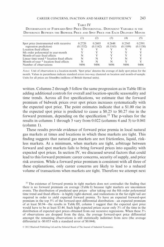
written. Columns 2 through 5 follow the same progression as in Table III inadding additional controls for overall and location-specific seasonality andtime trends. Across all five specifications, we estimate that the forwardpremium of bidweek prices over spot prices increases systematically withthe expected spot price. The point estimates indicate that a $1.00 rise inthe expected spot price is predicted to cause a $0.25 to $0.27 rise in theforward premium, depending on the specification.33 The p-values for theresults in columns 1 through 5 vary from 0.022 (columns 4 and 5) to 0.041(column 1).

These results provide evidence of forward price premia in local naturalgas markets at times and locations in which these markets are tight. Thisfinding suggests that natural gas markets are not frictionless, liquid, risk-less markets. At a minimum, when markets are tight, arbitrage betweenforward and spot markets fails to bring forward prices into equality withexpected spot prices. In section IV, we discussed several factors that couldlead to this forward premium: career concerns, security of supply, and pricerisk aversion. While a forward price premium is consistent with all three ofthese explanations, only career concerns are likely to lead to a reducedvolume of transactions when markets are tight. Therefore we attempt next

33 The existence of forward premia in tight markets does not contradict the finding thatthere is no forward premium on average (Table I) because tight markets are uncommonevents. The distribution of predicted spot prices—after taking out the 8th order polynomialtime trend and fixed effects—is highly right-skewed, and realizations in the far-right tail arerequired in order to yield expected forward premia. To have an expected forward-spotpremium in the top 5% of the forward-spot differential distribution—an expected premiumof at least $0.94—the results in Table III, column 1 suggest that the expected spot pricewould have to be at least $3.44. Such high expected prices occur only 3% of the time in thedistribution of expected spot prices obtained from our recursive regressions. When these 3%of observations are dropped from the data, the average forward-spot price differentialamongst the remaining observations is still statistically indistinct from zero (the averagedifferential is -$0.053 with a standard error of $0.044).

TABLE IVDETERMINANTS OF FORWARD-SPOT PRICE DIFFERENTIAL. DEPENDENT VARIABLE IS THE

DIFFERENCE BETWEEN THE BIDWEEK PRICE AND SPOT PRICE FOR EACH DELIVERY MONTH

(1) (2) (3) (4) (5)


0.2720 0.2603 0.2648 0.2545 0.2591(0.1332) (0.1142) (0.1163) (0.1109) (0.1130)

Location fixed effects Y Y Y Y Y8th order polynomial in year-month Y Y Y Y YMonth-of-year fixed effects N Y Y Y YLinear time trend * location fixed effects N N Y N YMonth-of-year * location fixed effects N N N Y YNumber of observations 9496 9496 9496 9496 9496




to distinguish amongst these theories, or at least assess which is dominant,by examining data on forward trading volumes in markets that are tightversus volumes in markets that are not tight.

VII(ii). Forward Trading Volumes

Column 1 of Table V reports the results of estimating equation [5] with thebidweek volume data. The estimated coefficient on the spot price demon-strates that forward trading volumes are significantly lower in tightmarkets. A $1.00 increase in the expected spot price is predicted to decreasethe logarithm of forward trading volume by 0.093, equivalent to a decreasein volume of 8.9%. The effect is statistically significant at the 1% level andis robust to the addition of additional controls for overall and location-specific seasonality and time trends.

An alternative explanation for these forward volume results is thatnatural gas trading simply becomes more difficult when markets aretight. For example, it may be that it becomes difficult to physically con-summate a trade when the gas delivery infrastructure is near its capa-city. However, if such a transactions cost story explains the decrease inforward trading volumes when markets are tight, then we should alsoobserve that spot trading volumes also decrease when markets are tight.The inaction model, on the other hand, does not imply decreases in spottrades. Thus, we can use data on spot trading volumes to distinguish thesetwo explanations.34

Platts’ spot market data provides observations of daily spot tradingvolumes, and we average these volumes within each location-month togenerate monthly time series of spot market volumes at each location. For

34 Another alternative hypothesis is that the correlation of shocks across utilities increasesin tight markets, lowering transactions volumes. Under this hypothesis, volumes shoulddecrease in both bidweek and spot markets, not just bidweek markets.

TABLE VDETERMINANTS OF LOG(BIDWEEK TRADING VOLUME)

(1) (2) (3) (4) (5)


-0.0931 -0.0956 -0.0837 -0.0961 -0.0830(0.0232) (0.0213) (0.0206) (0.0217) (0.0211)





comparability to the bidweek volume results, we use only location-monthsfor which bidweek volume data are also available. Spot volumes were notrecorded at 5 of these locations; the spot volume dataset therefore consistsof 4,324 observations spread over 69 locations.35 Summary statistics forspot volumes are given in Table I; these volumes are of similar magnitudesto those in the bidweek market.

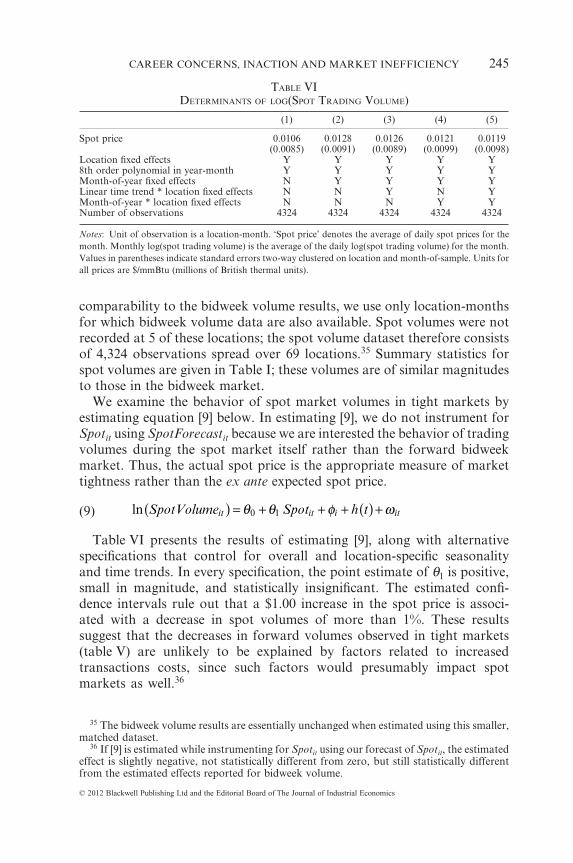
We examine the behavior of spot market volumes in tight markets byestimating equation [9] below. In estimating [9], we do not instrument forSpotit using SpotForecastit because we are interested the behavior of tradingvolumes during the spot market itself rather than the forward bidweekmarket. Thus, the actual spot price is the appropriate measure of markettightness rather than the ex ante expected spot price.

(9) ln SpotVolume Spot h tit it i it( ) = + + + ( ) +θ θ φ ω0 1

Table VI presents the results of estimating [9], along with alternativespecifications that control for overall and location-specific seasonalityand time trends. In every specification, the point estimate of q1 is positive,small in magnitude, and statistically insignificant. The estimated confi-dence intervals rule out that a $1.00 increase in the spot price is associ-ated with a decrease in spot volumes of more than 1%. These resultssuggest that the decreases in forward volumes observed in tight markets(table V) are unlikely to be explained by factors related to increasedtransactions costs, since such factors would presumably impact spotmarkets as well.36

35 The bidweek volume results are essentially unchanged when estimated using this smaller,matched dataset.

36 If [9] is estimated while instrumenting for Spotit using our forecast of Spotit, the estimatedeffect is slightly negative, not statistically different from zero, but still statistically differentfrom the estimated effects reported for bidweek volume.

TABLE VIDETERMINANTS OF LOG(SPOT TRADING VOLUME)

(1) (2) (3) (4) (5)

Spot price 0.0106 0.0128 0.0126 0.0121 0.0119(0.0085) (0.0091) (0.0089) (0.0099) (0.0098)


Notes: Unit of observation is a location-month. ‘Spot price’ denotes the average of daily spot prices for themonth. Monthly log(spot trading volume) is the average of the daily log(spot trading volume) for the month.Values in parentheses indicate standard errors two-way clustered on location and month-of-sample. Units forall prices are $/mmBtu (millions of British thermal units).



The implication of these results is that trade in forward markets isreduced when spot prices are expected to be high. This outcome suggeststhat there is a market inefficiency at work: forward markets shrink at thevery time they are most needed. These reductions in forward quantitiestraded are consistent with the inaction model in which the regulator penal-izes supply shortfalls caused by forward sales more than shortfalls causedby insufficient forward purchases. Absent the behavior caused by thisregulatory asymmetry, a model of security of supply concerns alone wouldnot predict the observed effects, nor would a model of price-risk aversion.

VIII. CONCLUSION AND BROADER RELEVANCE

We have presented a model of natural gas procurement by regulated utili-ties in which career concerns between the utilites and their regulators leadto an incentive for inaction in forward natural gas markets. In particular, in‘tight’ market situations in which customer demand is expected to be highin the near-term, career concerns can lead a utility to be unwilling to sell gasin the forward market, even when the forward price exceeds the expectedspot price over the upcoming month. This incentive for inaction derivesfrom the possibility that a positive demand shock might force the utility tobuy gas in the spot market at an extremely high price or even curtail itscustomers. When such an outcome can be linked to a sale of gas in theforward market, it will diminish the utility’s reputation and may lead to aparticularly harsh punishment by the regulator.

When several utilities in an area face career concerns and incentives forinaction, a forward price premium and a decrease in forward trade result.The incentive for inaction and commensurate reduction in trade is mostsalient in tight gas markets, as we verify empirically. Unfortunately, it is insuch situations that trade is most valuable: demand is expected to be highand there may be a large increase in social surplus from transferring gas tothose utilities that value it most.

As career concerns and problems of essential input procurement arehardly unique to the natural gas industry, we suspect that incentives forinaction may exist in other settings as well. Agents’ responses to theseincentives in aggregate can have significant market repercussions. Forexample, a procurement agent within a firm may carry excess inventoriesof inputs so (s)he can never be blamed for a disruption in the productionprocess. In aggregate, this behavior would distort allocation of the inputsamong input customers. Likewise, an agent might stick to historical sourc-ing when a new vendor would have higher expected value for the firm(‘nobody ever got fired for buying IBM’). Again, in aggregate such behav-ior could make it difficult for a new input supplier to enter the market.Finally, human resource managers in an industry might prefer to selectexcessively conventional job candidates, thereby in aggregate discouraging



people of less conventional talents or backgrounds from investing in theskills to enter the industry.

The imposition of particularly harsh penalties for observable actions thatcan be linked to negative outcomes may be efficient from the principal’spoint of view, suggesting that rational managers in an organization may bewilling to apply them. However, we demonstrate that the impacts of theseincentives extend beyond the principal-agent relationship in which theyare applied and can cause significant market inefficiencies. In markets fornecessary inputs, the career concerns generated by these principal-agentrelationships can cause firms to be reluctant to engage in trades, even whendifferences in marginal valuations are significant.

REFERENCES

Borenstein, S.; Busse, M. and Kellogg, R., 2007, ‘Principal-Agent Incentives, ExcessCaution and Market Inefficiency: Evidence from Utility Regulation,’ Center for theStudy of Energy Markets Working Paper No. 174 (University of California EnergyInstitute, 2547 Channing Way, Berkeley, California, U.S.A.).

Brandenburger, A. and Polak, B. 1996, ‘When Managers Cover their Posteriors:Making Decisions the Market Wants to See,’ RAND Journal of Economics, 27(3),pp. 523–541.

Cameron, A.C.; Gelbach, J. and Miller, D. 2011, ‘Robust Inference with Multi-WayClustering,’ Journal of Business and Economic Statistics, 28(2), pp. 238–249.

Chevalier, J. and Ellison, G. 1999, ‘Career Concerns of Mutual Fund Managers,’Quarterly Journal of Economics, 114(2), pp. 389–432.

Costello, K.W. and Cita, J. 2001, ‘Use of Hedging by Local Gas Distribution Compa-nies: Basic Considerations and Regulatory Issues,’ The National RegulatoryResearch Institute report NRRI No. 01–08 (National Regulatory Research Institute,8730 Georgia Avenue no. 201, Silver Spring, Maryland, U.S.A.).

Dasgupta, A. and Prat, A. 2008, ‘Information Aggregation in Financial Markets withCareer Concerns,’ Journal of Economic Theory, 143(1), pp. 83–113.

Greene, W. 2004. ‘Fixed Effects and Bias Due to the Incidental Parameters Problem inthe Tobit Model,’ Econometric Reviews, 23(2), pp. 125–147.

Guerrieri, V. and Kondor, P. 2009, ‘Fund Managers, Career Concerns, and AssetPrice Volatility,’ National Bureau of Economic Research working paper No. 14898(National Bureau of Economic Research, Inc., 1050 Massachusetts Avenue,Cambridge, Massachusetts, U.S.A.).

Harbaugh, R., 2006, ‘Prospect Theory or Skill Signaling?’ Working Papers 2005–06(Indiana University, Kelley School of Business, Department of Business Economicsand Public Policy, 1275 E. 10th Street, Bloomington, Indiana, U.S.A.).

Holmstrom, B. 1982/1999, ‘Managerial Incentive Problems: A Dynamic Perspective,’Festschrift für Lars Wahlback [1982], republished in 1999 in Review of EconomicStudies, 66(1), pp. 169–182.

Murphy, K.M. and Topel, R.H. 1985, ‘Estimation and Inference in Two-StepEconometric Models,’ Journal of Business and Economic Statistics, 3(4), pp. 370–379.

National Association of Regulatory Utility Commissioners. 2008, ‘Natural Gas Infor-mation Toolkit.’ (NARUC, 1101 Vermont Avenue, N.W., Suite 200, Washington,D.C., U.S.A.).



Neyman, J and Scott, E.L. 1948. ‘Consistent Estimates Based on Partially ConsistentObservations,’ Econometrica, 16(1), pp. 1–32.

Prendergast, C. and Stole, L. 1996, ‘Impetuous Youngsters and Jaded Old-Timers:Acquiring a Reputation for Learning,’ Journal of Political Economy, 104(6), pp.1105–1134.

Rajan, R.G. 1994, ‘Why Bank Credit Policies Fluctuate: A Theory and Some Evidence,’Quarterly Journal of Economics, 109(2), pp. 399–441.

Scharfstein, D.S. and Stein, J.C. 1990, ‘Herd Behavior and Investment,’ AmericanEconomic Review, 80(3), pp. 465–479.



Documents

Career Concerns, Inaction and Market Inefficiency: Evidence From Utility Regulation