Embed Size (px)
Citation preview
Cardiovascular Fluid Mechanics
- lecture notes 8W090 -
F.N. van de Vosse (2013)
Eindhoven University of Technologydepartment of Biomedical Engineering

Preface i
Preface
As cardiovascular disease is a major cause of death in the western world, knowledgeof cardiovascular pathologies, including heart valve failure and atherosclerosis is ofgreat importance. This knowledge can only be gathered after well understandingthe circulation of the blood. Also for the development and usage of diagnostic tech-niques, like ultrasound and magnetic resonance assessment of blood flow and vesselwall displacement, knowledge of the fluid mechanics of the circulatory system is in-dispensable. Moreover, awareness of cardiovascular fluid mechanics is of great helpin endovascular treatment of diseased arteries, the design of vascular prostheses thatcan replace these arteries when treatment is not successful, and in the developmentof prosthetic heart valves. Finally, development and innovation of extra-corporalsystems strongly relies on insight into cardiovascular fluid mechanics. The lecturenotes focus on fluid mechanical phenomena that occur in the human cardiovascularsystem and aim to contribute to better understanding of the circulatory system.
ii Cardiovascular Fluid Mechanics - lecture notes
In the introductory part of these notes a short overview of the circulatory systemwith respect to blood flow and pressure will be given. In chapter 1 a simple modelof the vascular system will be presented despite the fact that the fluid mechanics ofthe cardiovascular system is complex due to the non-linear and non-homogeneousrheological properties of blood and arterial wall, the complex geometry and thepulsatile flow properties.An important part, chapter 2, is dedicated to the description of Newtonian flowin straight, curved and bifurcating, rigid tubes. With the aid of characteristic di-mensionless parameters the flow phenomena will be classified and related to specificphysiological phenomena in the cardiovascular system. In this way difference be-tween flow in the large arteries and flow in the micro-circulation and veins and thedifference between flow in straight and curved arteries will be elucidated. It will beshown that the flow in branched tubes shows a strong resemblance to the flow incurved tubes.Although flow patterns as derived from rigid tube models do give a good approx-imation of those that can be found in the vascular system, they will not provideinformation on pressure pulses and wall motion. In order to obtain this informa-tion a short introduction to vessel wall mechanics will be given and models for wallmotion of distensible tubes as a function of a time dependent pressure load will bederived in chapter 3.The flow in distensible tubes is determined by wave propagation of the pressurepulse. The main characteristics of the wave propagation including attenuation andreflection of waves at geometrical transitions are treated in chapter 4, using a one-dimensional wave propagation model.As blood is a fluid consisting of blood cells suspended in plasma its rheologicalproperties differ from that of a Newtonian fluid. In chapter 5 constitutive equationsfor Newtonian flow, generalized Newtonian flow, viscoelastic flow and the flow ofsuspensions will be dealt with. It will be shown that the viscosity of blood is shearand history dependent as a result of the presence of deformation and aggregation ofthe red blood cells that are suspended in plasma. The importance of non-Newtonianproperties of blood for the flow in large and medium sized arteries will be discussed.Finally in chapter 6 the importance of the rheological (non-Newtonian) properties ofblood, and especially its particulate character, for the flow in the micro-circulationwill be elucidated. Velocity profiles as a function of the ratio between the vesseldiameter and the diameter of red blood cells will be derived.In the appendix A, a short review of the equations governing fluid mechanics isgiven. This includes the main concepts determining the constitutive equations forboth fluids and solids. Using limiting values of the non-dimensional parameters,simplifications of these equations will be derived in subsequent chapters.In order to obtain a better understanding of the physical meaning, many of themathematical models that are treated are implemented in MATLAB. Descriptionsof these implementations are available in a separate manuscript: ’CardiovascularFluid Mechanics - computational models’.
Contents
1 General introduction 1
1.1 Introduction . . . . . . . . . . . . . . . . . . . . . . . . . . . . . . . . 1
1.2 The cardiovascular system . . . . . . . . . . . . . . . . . . . . . . . . 2
1.2.1 The heart . . . . . . . . . . . . . . . . . . . . . . . . . . . . . 3
1.2.2 The systemic circulation . . . . . . . . . . . . . . . . . . . . . 7
1.3 Pressure and flow in the cardiovascular system . . . . . . . . . . . . 9
1.3.1 Pressure and flow waves in arteries . . . . . . . . . . . . . . . 9
1.3.2 Pressure and flow in the micro-circulation . . . . . . . . . . . 13
1.3.3 Pressure and flow in the venous system . . . . . . . . . . . . 13
1.4 Simple model of the vascular system . . . . . . . . . . . . . . . . . . 13
1.4.1 Periodic deformation and flow . . . . . . . . . . . . . . . . . . 13
1.4.2 The windkessel model . . . . . . . . . . . . . . . . . . . . . . 14
1.4.3 Vascular impedance . . . . . . . . . . . . . . . . . . . . . . . 15
1.5 Summary . . . . . . . . . . . . . . . . . . . . . . . . . . . . . . . . . 16
2 Newtonian flow in blood vessels 17
2.1 Introduction . . . . . . . . . . . . . . . . . . . . . . . . . . . . . . . . 17
2.2 Steady and pulsatile Newtonian flow in straight tubes . . . . . . . . 18
2.2.1 Fully developed flow . . . . . . . . . . . . . . . . . . . . . . . 18
2.2.2 Entrance flow . . . . . . . . . . . . . . . . . . . . . . . . . . . 25
2.3 Steady and pulsating flow in curved and branched tubes . . . . . . . 27
2.3.1 Steady flow in a curved tube . . . . . . . . . . . . . . . . . . 27
2.3.2 Unsteady fully developed flow in a curved tube . . . . . . . . 33
2.3.3 Flow in branched tubes . . . . . . . . . . . . . . . . . . . . . 35
2.4 Summary . . . . . . . . . . . . . . . . . . . . . . . . . . . . . . . . . 35
3 Mechanics of the vessel wall 37
3.1 Introduction . . . . . . . . . . . . . . . . . . . . . . . . . . . . . . . . 37
3.2 Morphology . . . . . . . . . . . . . . . . . . . . . . . . . . . . . . . . 38
3.3 Mechanical properties . . . . . . . . . . . . . . . . . . . . . . . . . . 39
3.4 Incompressible elastic deformation . . . . . . . . . . . . . . . . . . . 42
3.4.1 Deformation of incompressible linear elastic solids . . . . . . 42
3.4.2 Approximation for small strains . . . . . . . . . . . . . . . . . 43
3.5 Wall motion . . . . . . . . . . . . . . . . . . . . . . . . . . . . . . . . 45
3.6 Summary . . . . . . . . . . . . . . . . . . . . . . . . . . . . . . . . . 47
iii
iv Cardiovascular Fluid Mechanics - lecture notes
4 Wave phenomena in blood vessels 49
4.1 Introduction . . . . . . . . . . . . . . . . . . . . . . . . . . . . . . . . 49
4.2 Pressure and flow . . . . . . . . . . . . . . . . . . . . . . . . . . . . . 50
4.3 Fluid flow . . . . . . . . . . . . . . . . . . . . . . . . . . . . . . . . . 51
4.4 Wave propagation . . . . . . . . . . . . . . . . . . . . . . . . . . . . 53
4.4.1 Derivation of a quasi one-dimensional model . . . . . . . . . 53
4.4.2 Wave speed and attenuation constant . . . . . . . . . . . . . 56
4.5 Wave reflection . . . . . . . . . . . . . . . . . . . . . . . . . . . . . . 61
4.5.1 Wave reflection at discrete transitions . . . . . . . . . . . . . 61
4.5.2 Multiple wave reflection: effective admittance . . . . . . . . . 64
4.5.3 Vascular impedance and cardiac work . . . . . . . . . . . . . 67
4.6 Summary . . . . . . . . . . . . . . . . . . . . . . . . . . . . . . . . . 68
5 Non-Newtonian flow in blood vessels 69
5.1 Introduction . . . . . . . . . . . . . . . . . . . . . . . . . . . . . . . . 69
5.2 Mechanical properties of blood . . . . . . . . . . . . . . . . . . . . . 70
5.2.1 Morphology . . . . . . . . . . . . . . . . . . . . . . . . . . . . 70
5.2.2 Rheological properties of blood . . . . . . . . . . . . . . . . . 72
5.3 Newtonian models . . . . . . . . . . . . . . . . . . . . . . . . . . . . 75
5.3.1 Constitutive equations . . . . . . . . . . . . . . . . . . . . . . 75
5.3.2 Viscometric results . . . . . . . . . . . . . . . . . . . . . . . . 76
5.4 Generalized Newtonian models . . . . . . . . . . . . . . . . . . . . . 76
5.4.1 Constitutive equations . . . . . . . . . . . . . . . . . . . . . . 76
5.4.2 Viscometric results . . . . . . . . . . . . . . . . . . . . . . . . 77
5.5 Viscoelastic models . . . . . . . . . . . . . . . . . . . . . . . . . . . . 80
5.5.1 Constitutive equations . . . . . . . . . . . . . . . . . . . . . . 80
5.5.2 Viscometric results . . . . . . . . . . . . . . . . . . . . . . . . 83
5.6 Rheology of suspensions . . . . . . . . . . . . . . . . . . . . . . . . . 86
5.6.1 Constitutive equations . . . . . . . . . . . . . . . . . . . . . . 86
5.6.2 Viscometric results . . . . . . . . . . . . . . . . . . . . . . . . 88
5.7 Rheology of whole blood . . . . . . . . . . . . . . . . . . . . . . . . . 88
5.7.1 Experimental observations . . . . . . . . . . . . . . . . . . . . 88
5.7.2 Constitutive equations . . . . . . . . . . . . . . . . . . . . . . 90
5.8 Summary . . . . . . . . . . . . . . . . . . . . . . . . . . . . . . . . . 91
6 Flow patterns in the micro-circulation 93
6.1 Introduction . . . . . . . . . . . . . . . . . . . . . . . . . . . . . . . . 93
6.2 Flow in small arteries and small veins: Dv > 2Dc . . . . . . . . . . . 94
6.3 Velocity profiles . . . . . . . . . . . . . . . . . . . . . . . . . . . . . . 94
6.3.1 Flow . . . . . . . . . . . . . . . . . . . . . . . . . . . . . . . . 96
6.3.2 Effective viscosity . . . . . . . . . . . . . . . . . . . . . . . . 96
6.3.3 Concentration . . . . . . . . . . . . . . . . . . . . . . . . . . . 97
6.3.4 Cell velocity . . . . . . . . . . . . . . . . . . . . . . . . . . . . 98
6.4 Flow in arterioles and venules : Dc < Dv < 2Dc . . . . . . . . . . . . 98
6.4.1 Velocity profiles . . . . . . . . . . . . . . . . . . . . . . . . . . 98
6.4.2 Flow . . . . . . . . . . . . . . . . . . . . . . . . . . . . . . . . 98
Contents v
6.4.3 Effective viscosity . . . . . . . . . . . . . . . . . . . . . . . . 996.4.4 Concentration . . . . . . . . . . . . . . . . . . . . . . . . . . . 996.4.5 Cell velocity . . . . . . . . . . . . . . . . . . . . . . . . . . . . 100
6.5 Flow in capillaries: Dv < Dc . . . . . . . . . . . . . . . . . . . . . . . 1006.6 Summary . . . . . . . . . . . . . . . . . . . . . . . . . . . . . . . . . 102
A Basic equations 103
A.1 Introduction . . . . . . . . . . . . . . . . . . . . . . . . . . . . . . . . 103A.2 The state of stress and deformation . . . . . . . . . . . . . . . . . . . 104
A.2.1 Stress . . . . . . . . . . . . . . . . . . . . . . . . . . . . . . . 104A.2.2 Displacement and deformation . . . . . . . . . . . . . . . . . 104A.2.3 Velocity and rate of deformation . . . . . . . . . . . . . . . . 107A.2.4 Constitutive equations . . . . . . . . . . . . . . . . . . . . . . 108
A.3 Equations of motion . . . . . . . . . . . . . . . . . . . . . . . . . . . 109A.3.1 Reynolds’ transport theorem . . . . . . . . . . . . . . . . . . 109A.3.2 Continuity equation . . . . . . . . . . . . . . . . . . . . . . . 110A.3.3 The momentum equation . . . . . . . . . . . . . . . . . . . . 111A.3.4 Initial and boundary conditions . . . . . . . . . . . . . . . . . 112
A.4 Incompressible viscous flow . . . . . . . . . . . . . . . . . . . . . . . 112A.4.1 Newtonian flow . . . . . . . . . . . . . . . . . . . . . . . . . . 112
A.5 Incompressible in-viscid flow . . . . . . . . . . . . . . . . . . . . . . . 113A.5.1 Irotational flow . . . . . . . . . . . . . . . . . . . . . . . . . . 114A.5.2 Boundary conditions . . . . . . . . . . . . . . . . . . . . . . . 115
A.6 Incompressible boundary layer flow . . . . . . . . . . . . . . . . . . . 115A.6.1 Newtonian boundary layer flow . . . . . . . . . . . . . . . . . 115A.6.2 Initial and boundary conditions . . . . . . . . . . . . . . . . . 116

vi Cardiovascular Fluid Mechanics - lecture notes
Chapter 1
General introduction
1.1 Introduction
The study of cardiovascular fluid mechanics is only possible with some knowledgeof cardiovascular physiology. In this chapter a brief introduction to cardiovascularphysiology will be given. Some general aspects of the fluid mechanics of the heart,the arterial system, the micro-circulation and the venous system as well as themost important properties of the vascular tree that determine the pressure and flowcharacteristics in the cardiovascular system will be dealt with. Although the fluidmechanics of the vascular system is complex due to complexity of geometry andpulsatility of the flow, a simple linear model of this system will be derived.
1
2 Cardiovascular Fluid Mechanics - lecture notes
1.2 The cardiovascular system
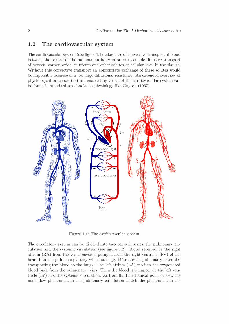
The cardiovascular system (see figure 1.1) takes care of convective transport of bloodbetween the organs of the mammalian body in order to enable diffusive transportof oxygen, carbon oxide, nutrients and other solutes at cellular level in the tissues.Without this convective transport an appropriate exchange of these solutes wouldbe impossible because of a too large diffusional resistance. An extended overview ofphysiological processes that are enabled by virtue of the cardiovascular system canbe found in standard text books on physiology like Guyton (1967).
pa
pv
head, arms
liver, kidneys
legs
lungs
stomach, gut
Figure 1.1: The cardiovascular system
The circulatory system can be divided into two parts in series, the pulmonary cir-culation and the systemic circulation (see figure 1.2). Blood received by the rightatrium (RA) from the venae cavae is pumped from the right ventricle (RV) of theheart into the pulmonary artery which strongly bifurcates in pulmonary arteriolestransporting the blood to the lungs. The left atrium (LA) receives the oxygenatedblood back from the pulmonary veins. Then the blood is pumped via the left ven-tricle (LV) into the systemic circulation. As from fluid mechanical point of view themain flow phenomena in the pulmonary circulation match the phenomena in the
General Introduction 3
systemic circulation, in the sequel of this course only the systemic circulation willbe considered.
pulmonary
circulationsystemic
circulation
aorta
a. pulmonaris
RA LAv.cava
RV LV
v.pulmonaris
aortic valve
mitral valve
tricuspid valve
pulmonary valve
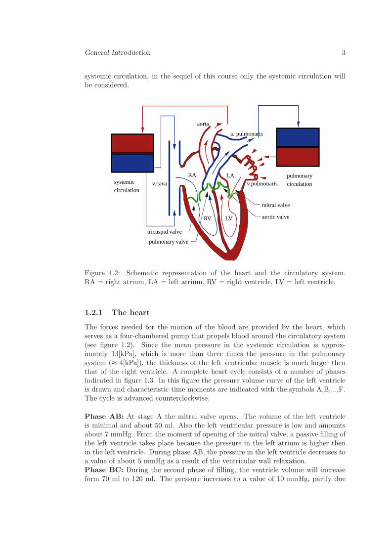
Figure 1.2: Schematic representation of the heart and the circulatory system.RA = right atrium, LA = left atrium, RV = right ventricle, LV = left ventricle.
1.2.1 The heart
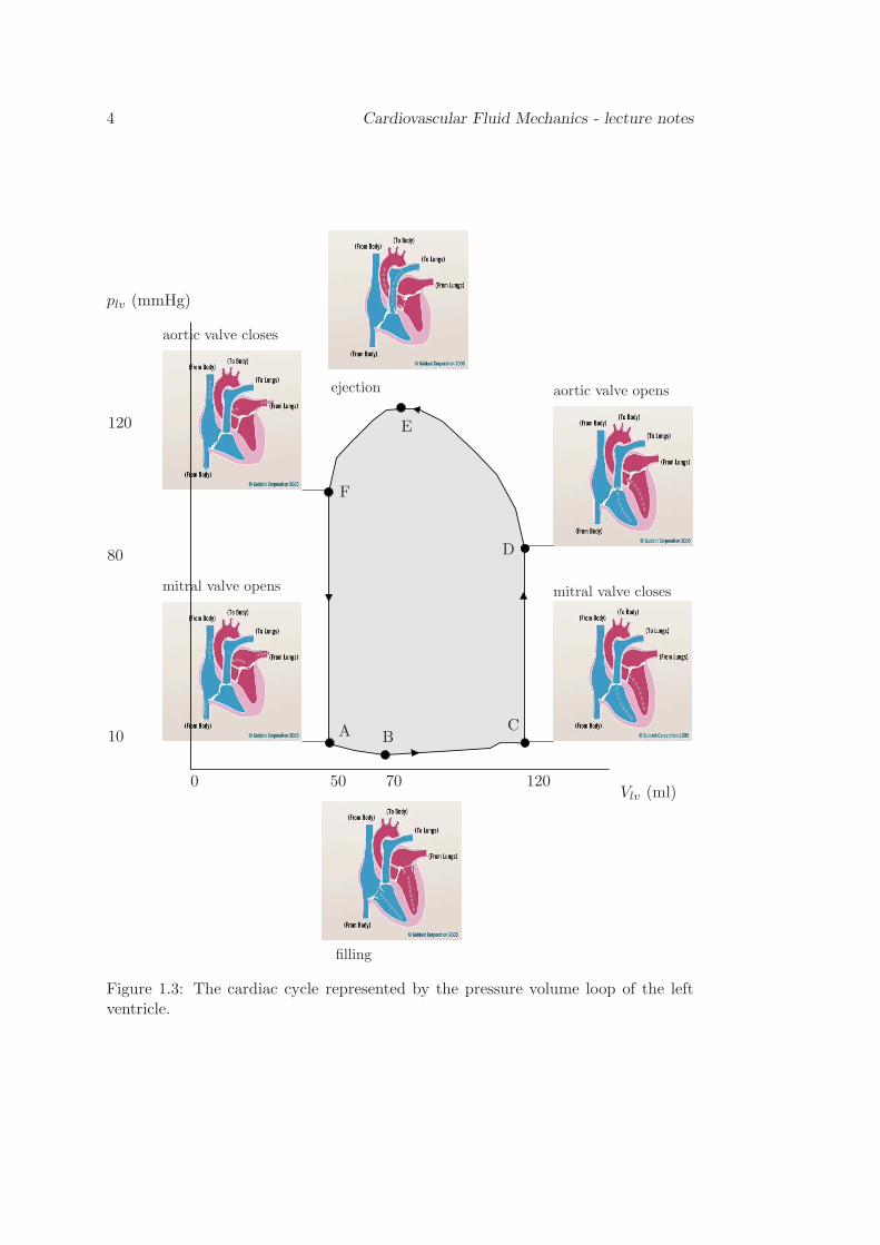
The forces needed for the motion of the blood are provided by the heart, whichserves as a four-chambered pump that propels blood around the circulatory system(see figure 1.2). Since the mean pressure in the systemic circulation is approx-imately 13[kPa], which is more than three times the pressure in the pulmonarysystem (≈ 4[kPa]), the thickness of the left ventricular muscle is much larger thenthat of the right ventricle. A complete heart cycle consists of a number of phasesindicated in figure 1.3. In this figure the pressure volume curve of the left ventricleis drawn and characteristic time moments are indicated with the symbols A,B,...,F.The cycle is advanced counterclockwise.
Phase AB: At stage A the mitral valve opens. The volume of the left ventricleis minimal and about 50 ml. Also the left ventricular pressure is low and amountsabout 7 mmHg. From the moment of opening of the mitral valve, a passive filling ofthe left ventricle takes place because the pressure in the left atrium is higher thenin the left ventricle. During phase AB, the pressure in the left ventricle decreases toa value of about 5 mmHg as a result of the ventricular wall relaxation.Phase BC: During the second phase of filling, the ventricle volume will increaseform 70 ml to 120 ml. The pressure increases to a value of 10 mmHg, partly due
4 Cardiovascular Fluid Mechanics - lecture notes
plv (mmHg)
Vlv (ml)0
10
50 70
80
120
120
aortic valve opens
aortic valve closes
mitral valve opens mitral valve closes
filling
ejection
A BC
D
E
F
Figure 1.3: The cardiac cycle represented by the pressure volume loop of the leftventricle.
General Introduction 5
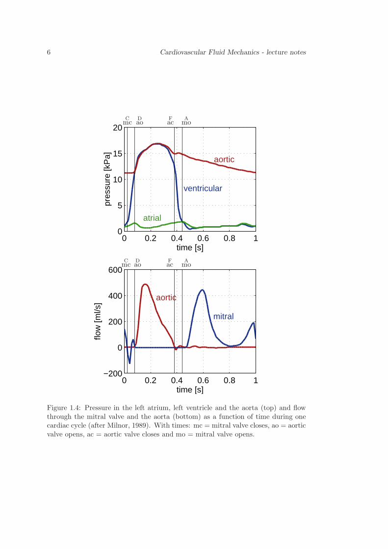
to the contraction of the atrium at the end of this phase induced by a stimulus formuscle contraction of the sinoatrial node.Phase CD: This phase starts with the closure of the mitral valve induced by theincrease pressure in the ventricle. Both the mitral and aortic valve are closed. Due tothe incompressibility of the blood inside the ventricle the volume of approximately120 ml will not change. In this phase also the contraction of the left ventriclestarts, controlled by a stimulus generated by the atrioventricular node, resulting ina pressure rapidly increasing from 10 mmHg to 80 mmHg. This phase is called theisovolumetric contraction.Phase DE: This phase starts when the aortic valve opens due to the fact thatthe ventricular pressure has become larger then the aortic pressure. As blood flowvrom the ventricle into the aorta, ventriclular volume decreases with an amount ofabout 45 ml. The pressure is still increasing as a result of the strong contractionand reaches its maximum value of 120 mmHg.Phase EF: At stage E the contraction of the heart starts to loose its strength andthe ventricular pressure decreases from 120 mmHg to about 100 mmHg. The bloodflowing through the aortic valve is decelerated until the moment that the aortic valvecloses at stage F. The volume of the ventricle then has reached its minimum valueof about 50 ml.Phase FA: This is the isovolumetric relaxation. Both valves are close and thecardiac muscle relaxes. As a result the pressure rapidly decreases from 100 mmHgto 10 mmHg at stage A.Note that the phases described above are not all of the same length. This becomesclear if we look at the ventricular and aortic pressure and aortic flow as a functionof time during the cardiac cycle as given in figure 1.4. The mitral valve opens (mo)at stage A and until the mitral valve closes (mc), atrial pressure and contractioncauses a filling of the ventricles with hardly any increase of the ventricular pressure.In the left heart the mitral valve is opened and offers very low resistance. The aorticvalve is closed. Shortly after this, at the onset of systole the two ventricles contractsimultaneously. At the same time the mitral valve closes (mc) and a sharp pressurerise in the left ventricle occurs. At the moment that this ventricular pressure exceedsthe pressure in the aorta, the aortic valve opens (ao) and blood is ejected into theaorta. The ventricular and aortic pressure first rise and then fall as a result of acombined action of ventricular contraction forces and the resistance and complianceof the systemic circulation. Due to this pressure fall (or actually the correspondingflow deceleration) the aortic valve closes (ac) and the pressure in the ventricle dropsrapidly, the mitral valve opens (mo), while the heart muscle relaxes (diastole).Since, in the heart, both the blood flow velocities as well as the geometrical lengthscales are relatively large, the fluid mechanics of the heart is strongly determined byinertial forces which are in equilibrium with pressure forces.
6 Cardiovascular Fluid Mechanics - lecture notes
0 0.2 0.4 0.6 0.8 10
5
10
15
20
time [s]
pres
sure
[kP
a]
atrial
aortic
ventricular
0 0.2 0.4 0.6 0.8 1−200
0
200
400
600
time [s]
flow
[ml/s
] aortic
mitral
Amo
Amo
Cmc
Cmc
Dao
Dao
Fac
Fac
Figure 1.4: Pressure in the left atrium, left ventricle and the aorta (top) and flowthrough the mitral valve and the aorta (bottom) as a function of time during onecardiac cycle (after Milnor, 1989). With times: mc = mitral valve closes, ao = aorticvalve opens, ac = aortic valve closes and mo = mitral valve opens.
General Introduction 7
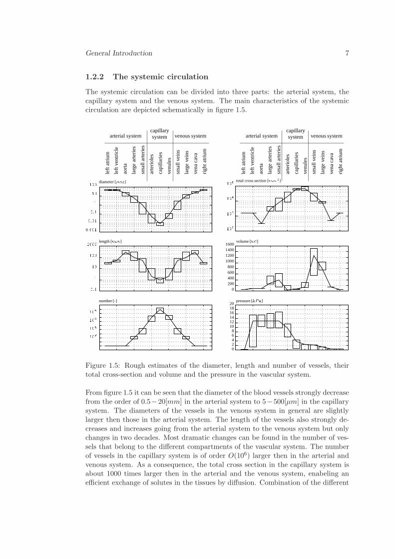
1.2.2 The systemic circulation
The systemic circulation can be divided into three parts: the arterial system, thecapillary system and the venous system. The main characteristics of the systemiccirculation are depicted schematically in figure 1.5.
1102104106108 number [-]
0:11101001000 length [mm]
1101000:0010:010:1 diameter [mm]
sma
lla
rte
ries
sma
llve
ins
larg
eve
ins
ven
aca
va
righ
tatr
ium
left
ven
tric
le
ao
rta
larg
ea
rte
ries
art
erio
les
cap
illa
ries
ven
ule
s
left
atr
ium
arterial systemcapillarysystem venous system
102103104105 total cross section [mm2]
0200400600800
1000120014001600
volume [ml]02468
101214161820
pressure [kPa]
sma
lla
rte
ries
sma
llve
ins
larg
eve
ins
ven
aca
va
righ
tatr
ium
left
ven
tric
le
ao
rta
larg
ea
rte
ries
art
erio
les
cap
illa
ries
ven
ule
s
left
atr
ium
arterial systemcapillarysystem venous system
Figure 1.5: Rough estimates of the diameter, length and number of vessels, theirtotal cross-section and volume and the pressure in the vascular system.
From figure 1.5 it can be seen that the diameter of the blood vessels strongly decreasefrom the order of 0.5−20[mm] in the arterial system to 5−500[µm] in the capillarysystem. The diameters of the vessels in the venous system in general are slightlylarger then those in the arterial system. The length of the vessels also strongly de-creases and increases going from the arterial system to the venous system but onlychanges in two decades. Most dramatic changes can be found in the number of ves-sels that belong to the different compartments of the vascular system. The numberof vessels in the capillary system is of order O(106) larger then in the arterial andvenous system. As a consequence, the total cross section in the capillary system isabout 1000 times larger then in the arterial and the venous system, enabeling anefficient exchange of solutes in the tissues by diffusion. Combination of the different
8 Cardiovascular Fluid Mechanics - lecture notes
dimensions mentioned above shows that the total volume of the venous system isabout 2 times larger then the volume of the arterial system and much larger thenthe total volume of the capillary system. As can be seen from the last figure, themean pressure falls gradually as blood flows into the systemic circulation. The pres-sure amplitude, however, shows a slight increase in the proximal part of the arterialsystem.
The arterial system is responsible for the transport of blood to the tissues. Be-sides the transport function of the arterial system the pulsating flow produced bythe heart is also transformed to a more-or-less steady flow in the smaller arteries.Another important function of the arterial system is to maintain a relatively higharterial pressure. This is of importance for a proper functioning of the brain andkidneys. This pressure can be kept at this relatively high value because the distalend of the arterial system strongly bifurcates into vessels with small diameters (ar-terioles) and hereby forms a large peripheral resistance. The smooth muscle cells inthe walls are able to change the diameter and hereby the resistance of the arterioles.In this way the circulatory system can adopt the blood flow to specific parts inaccordance to momentary needs (vasoconstriction and vasodilatation). Normallythe heart pumps about 5 liters of blood per minute but during exercise the heartminute volume can increase to 25 liters. This is partly achieved by an increase ofthe heart frequency but is mainly made possible by local regulation of blood flowby vasoconstriction and vasodilatation of the distal arteries (arterioles). Unlike thesituation in the heart, in the arterial system, also viscous forces may become ofsignificant importance as a result of a decrease in characteristic velocity and lengthscales (diameters of the arteries).
Leaving the arterioles the blood flows into the capillary system, a network of smallvessels. The walls consist of a single layer of endothelial cells lying on a basementmembrane. Here an exchange of nutrients with the interstitial liquid in the tissuestakes place. In physiology, capillary blood flow is mostly referred to as micro circu-lation. The diameter of the capillaries is so small that the whole blood may not beconsidered as a homogeneous fluid anymore. The blood cells are moving in a singlefile (train) and strongly deform. The plasma acts as a lubrication layer. The fluidmechanics of the capillary system hereby strongly differs from that of the arterialsystem and viscous forces dominate over inertia forces in their equilibrium with thedriving pressure forces.
Finally the blood is collected in the venous system (venules and veins) in whichthe vessels rapidly merge into larger vessels transporting the blood back to the heart.The total volume of the venous system is much larger then the volume of the arterialsystem. The venous system provides a storage function which can be controlled byconstriction of the veins (venoconstriction) that enables the heart to increase thearterial blood volume. As the diameters in the venous system are of the same orderof magnitude as in the arterial system, inertia forces may become influential again.Both characteristic velocities and pressure amplitudes, however, are lower than inthe arterial system. As a consequence, in the venous system, instationary inertia
General Introduction 9
forces will be of less importance then in the arterial system. Moreover, the pressurein the venous system is that low that gravitational forces become of importance.
The geometrical dimensions referred to above and summarized in figure 1.5 showthat the vascular tree is highly bifurcating and will be geometrically complex. Flowphenomena related with curvature and bifurcation of the vessels (see chapter 2) cannot be neglected. As in many cases the length of the vessels is small compared tothe length needed for fully developed flow, also entrance flow must be included instudies of cardiovascular fluid mechanics.
1.3 Pressure and flow in the cardiovascular system
1.3.1 Pressure and flow waves in arteries
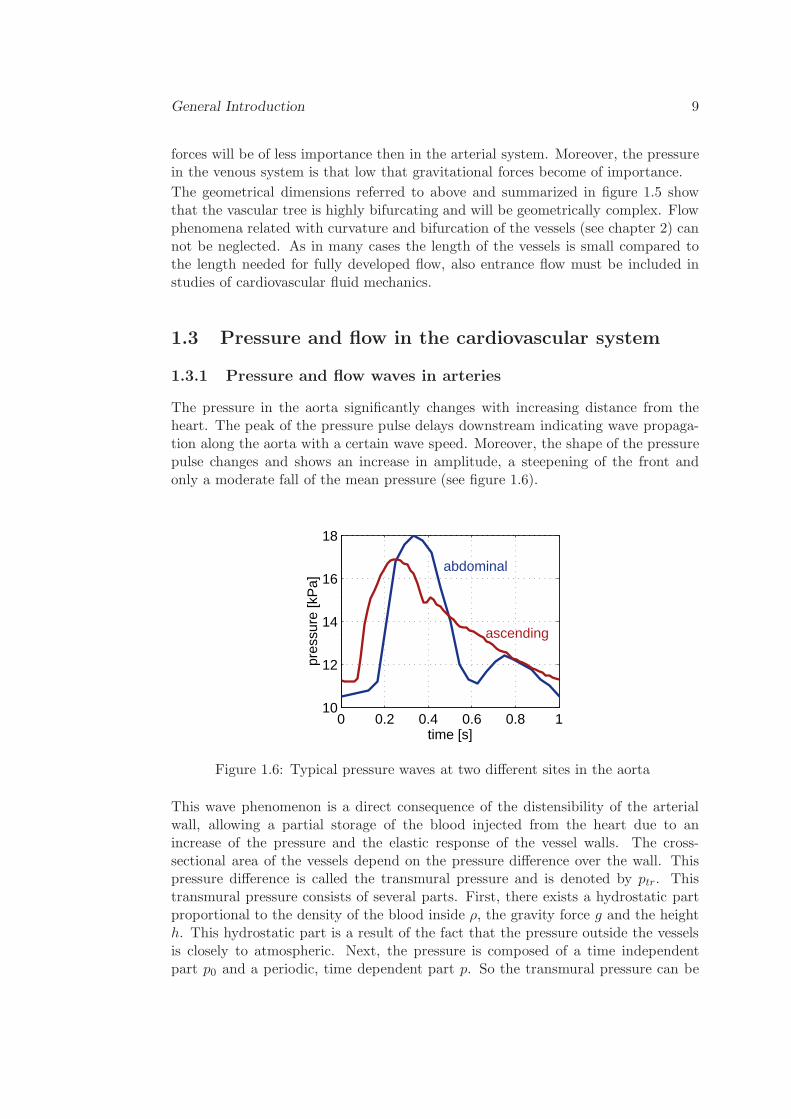
The pressure in the aorta significantly changes with increasing distance from theheart. The peak of the pressure pulse delays downstream indicating wave propaga-tion along the aorta with a certain wave speed. Moreover, the shape of the pressurepulse changes and shows an increase in amplitude, a steepening of the front andonly a moderate fall of the mean pressure (see figure 1.6).
0 0.2 0.4 0.6 0.8 110
12
14
16
18
time [s]
pres
sure
[kP
a]
abdominal
ascending
Figure 1.6: Typical pressure waves at two different sites in the aorta
This wave phenomenon is a direct consequence of the distensibility of the arterialwall, allowing a partial storage of the blood injected from the heart due to anincrease of the pressure and the elastic response of the vessel walls. The cross-sectional area of the vessels depend on the pressure difference over the wall. Thispressure difference is called the transmural pressure and is denoted by ptr. Thistransmural pressure consists of several parts. First, there exists a hydrostatic partproportional to the density of the blood inside ρ, the gravity force g and the heighth. This hydrostatic part is a result of the fact that the pressure outside the vesselsis closely to atmospheric. Next, the pressure is composed of a time independentpart p0 and a periodic, time dependent part p. So the transmural pressure can be
10 Cardiovascular Fluid Mechanics - lecture notes
written as:
ptr = ρqh+ p0 + p (1.1)
Due to the complex nonlinear anisotropic and viscoelastic properties of the arterialwall, the relation between the transmural pressure and the cross sectional area Aof the vessel is mostly nonlinear and can be rather complicated. Moreover it variesfrom one vessel to the other. Important quantities with respect to this relation, usedin physiology, are the compliance or alternatively the distensibility of the vessel.The compliance C is defined as:
C =∂A
∂p(1.2)
The distensibility D is defined by the ratio of the compliance and the cross sectionalarea and hereby is given by:
D =1
A
∂A
∂p=C
A(1.3)
In the sequel of this course these quantities will be related to the material propertiesof the arterial wall. For small diameter changes in thin walled tubes, with radius aand wall thickness h, without longitudinal strain, e.g., it can be derived that:
D =2a
h
1− µ2
E. (1.4)
Here µ denotes Poisson ’s ratio and E Young ’s modulus. From this we can see thatbesides the properties of the material of the vessel (E,µ) also geometrical properties(a, h) play an important role.The value of the ratio a/h varies strongly along the arterial tree. The veins are moredistensible than the arteries. Mostly, in some way, the pressure-area relationship,i.e. the compliance or distensibility, of the arteries or veins that are considered, haveto be determined from experimental data. A typical example of such data is givenin figure 1.7 where the relative transmural pressure p/p0 is given as a function of therelative cross-sectional area A/A0. As depicted in this figure, the compliance changeswith the pressure load since at relatively high transmural pressure, the collagen fibresin the vessel wall become streched and prevent the artery from further increase ofthe circumferential strain.The flow is driven by the gradient of the pressure and hereby determined by thepropagation of the pressure wave. Normally the pressure wave will have a pulsatingperiodic character. In order to describe the flow phenomena we distinguish betweensteady and unsteady part of this pulse. Often it is assumed that the unsteady partcan be described by means of a linear theory, so that we can introduce the conceptof pressure and flow waves which be superpositions of several harmonics:
p =N∑
n=1
pneniωt q =
N∑
n=1
qneniωt (1.5)
Here pn and qn are the complex Fourier coefficients and hereby p and q are thecomplex pressure and the complex flow, ω denotes the angular frequency of the
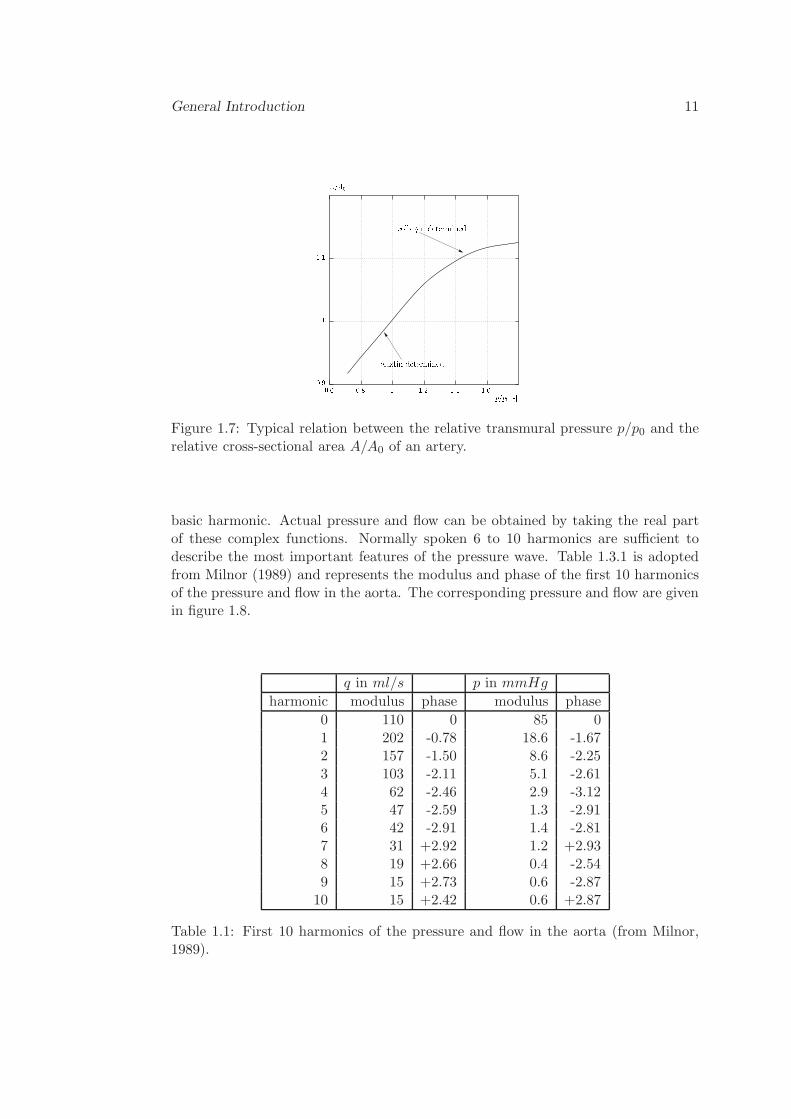
General Introduction 11
0.6 0.8 1 1.2 1.4 1.60.91
1.1p=p0 [-]
A=A0 [-]
elastin determinedcollagen determined
Figure 1.7: Typical relation between the relative transmural pressure p/p0 and therelative cross-sectional area A/A0 of an artery.
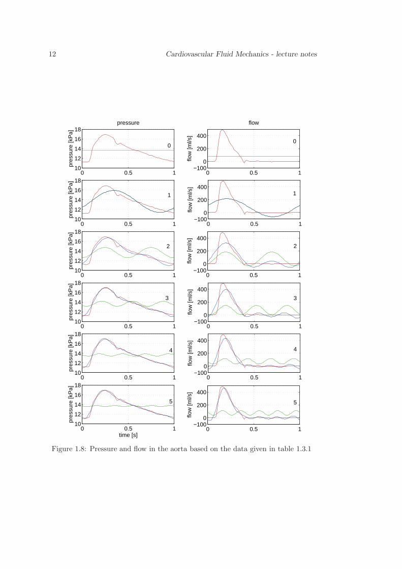
basic harmonic. Actual pressure and flow can be obtained by taking the real partof these complex functions. Normally spoken 6 to 10 harmonics are sufficient todescribe the most important features of the pressure wave. Table 1.3.1 is adoptedfrom Milnor (1989) and represents the modulus and phase of the first 10 harmonicsof the pressure and flow in the aorta. The corresponding pressure and flow are givenin figure 1.8.
q in ml/s p in mmHg
harmonic modulus phase modulus phase
0 110 0 85 01 202 -0.78 18.6 -1.672 157 -1.50 8.6 -2.253 103 -2.11 5.1 -2.614 62 -2.46 2.9 -3.125 47 -2.59 1.3 -2.916 42 -2.91 1.4 -2.817 31 +2.92 1.2 +2.938 19 +2.66 0.4 -2.549 15 +2.73 0.6 -2.8710 15 +2.42 0.6 +2.87
Table 1.1: First 10 harmonics of the pressure and flow in the aorta (from Milnor,1989).
12 Cardiovascular Fluid Mechanics - lecture notes
0 0.5 110
12
14
16
18
pres
sure
[kP
a]
0 0.5 1−100
0
200
400flo
w [m
l/s]
0 0.5 1−100
0
200
400
flow
[ml/s
]
0 0.5 1−100
0
200
400
flow
[ml/s
]
0 0.5 1−100
0
200
400
flow
[ml/s
]
0 0.5 1−100
0
200
400
flow
[ml/s
]
0 0.5 1−100
0
200
400
flow
[ml/s
]
flow
3
2
1
0
4
5
0 0.5 110
12
14
16
18
pres
sure
[kP
a]
1
0 0.5 110
12
14
16
18
pres
sure
[kP
a]
2
0 0.5 110
12
14
16
18
time [s]
pres
sure
[kP
a]
5
0 0.5 110
12
14
16
18
pres
sure
[kP
a]
pressure
0
0 0.5 110
12
14
16
18
pres
sure
[kP
a]
4
3
Figure 1.8: Pressure and flow in the aorta based on the data given in table 1.3.1
General Introduction 13
1.3.2 Pressure and flow in the micro-circulation
The micro-circulation is a strongly bifurcating network of small vessels and is re-sponsible for the exchange of nutrients and gases between the blood and the tissues.Mostly blood can leave the arterioles in two ways. The first way is to follow ametarteriole towards a specific part of the tissue and enter the capillary system.This second way is to bypass the tissue by entering an arterio venous anastomosisthat shortcuts the arterioles and the venules. Smooth muscle cells in the walls of themetarterioles, precapillary sphincters at the entrance of the capillaries and glomusbodies in the anastomoses regulate the local distribution of the flow. In contrastwith the arteries the pressure in the micro-vessels is more or less constant in timeyielding an almost steady flow. This steadiness, however, is strongly disturbed bythe ’control actions’ of the regulatory system of the micro-circulation. As the di-mensions of the blood cells are of the same order as the diameter of the micro-vesselsthe flow and deformation properties of the red cells must be taken into account inthe modeling of the flow in the micro-circulation (see chapter 2).
1.3.3 Pressure and flow in the venous system
The morphology of the systemic veins resemble arteries. The wall however is notas thick as in the arteries of the same diameter. Also the pressure in a vein ismuch lower than the pressure in an artery of the same size. In certain situationsthe pressure can be so low that in normal functioning the vein will have an ellipticcross-sectional area or even will be collapsed for some time. Apart from its differentwall thickness and the relatively low pressures, the veins distinguish from arteriesby the presence of valves to prevent back flow.
1.4 Simple model of the vascular system
1.4.1 Periodic deformation and flow
In cardiovascular fluid dynamics the flow often may be considered as periodic ifwe assume a constant duration of each cardiac cycle. In many cases, i.e. if thedeformation and the flow can be described by a linear theory, the displacements andvelocity can be decomposed in a number of harmonics using a Fourier transform:
v =N∑
n=0
vneinωt (1.6)
Here vn are the complex Fourier coefficients, ω denotes the angular frequency of thebasic harmonic. Note that a complex notation of the velocity is used exploiting therelation:
eiωt = cos(ωt) + i sin(ωt) (1.7)
with i =√−1. The actual velocity can be obtained by taking the real part of the
complex velocity. By substitution of relation (1.6) in the governing equations thatdescribe the flow, often an analytical solution can be derived for each harmonic.
14 Cardiovascular Fluid Mechanics - lecture notes
Superposition of these solution then will give a solution for any periodic flow as longas the equations are linear in the solution v.
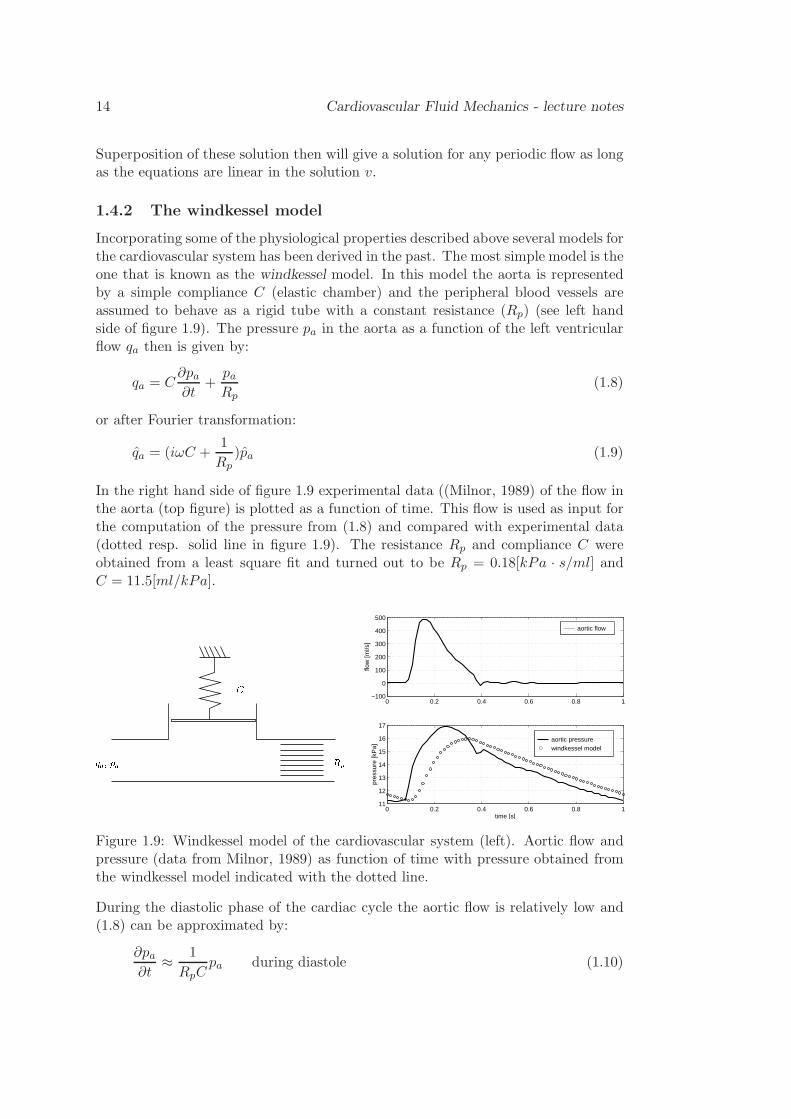
1.4.2 The windkessel model
Incorporating some of the physiological properties described above several models forthe cardiovascular system has been derived in the past. The most simple model is theone that is known as the windkessel model. In this model the aorta is representedby a simple compliance C (elastic chamber) and the peripheral blood vessels areassumed to behave as a rigid tube with a constant resistance (Rp) (see left handside of figure 1.9). The pressure pa in the aorta as a function of the left ventricularflow qa then is given by:
qa = C∂pa∂t
+paRp
(1.8)
or after Fourier transformation:
qa = (iωC +1
Rp)pa (1.9)
In the right hand side of figure 1.9 experimental data ((Milnor, 1989) of the flow inthe aorta (top figure) is plotted as a function of time. This flow is used as input forthe computation of the pressure from (1.8) and compared with experimental data(dotted resp. solid line in figure 1.9). The resistance Rp and compliance C wereobtained from a least square fit and turned out to be Rp = 0.18[kPa · s/ml] andC = 11.5[ml/kPa].
qa, paC
Rp
aortic flow
0 0.2 0.4 0.6 0.8 1−100
0
100
200
300
400
500
flow
[ml/s
]
aortic pressure windkessel model
0 0.2 0.4 0.6 0.8 111
12
13
14
15
16
17
time [s]
pres
sure
[kP
a]
Figure 1.9: Windkessel model of the cardiovascular system (left). Aortic flow andpressure (data from Milnor, 1989) as function of time with pressure obtained fromthe windkessel model indicated with the dotted line.
During the diastolic phase of the cardiac cycle the aortic flow is relatively low and(1.8) can be approximated by:
∂pa∂t
≈ 1
RpCpa during diastole (1.10)
General Introduction 15
with solution pa ≈ pase−t/RpC with pas peak systolic pressure. This approximate
solution resonably corresponds with experimental data.
During the systolic phase of the flow the aortic flow is much larger then the peripheralflow (qa ≫ pa/Rp) yielding:
∂pa∂t
≈ 1
Cqa during systole (1.11)
with solution pa ≈ pad+(1/C)∫
qadt with pad the diastolic pressure. Consequently aphase difference between pressure and flow is expected. Experimental data, however,show pa ≈ pad + kqa, so pressure and flow are more or less in-phase (see figure1.9). Notwithstanding the significant phase error in the systolic phase, this simplewindkessel model is often used to derive the cardiac work at given flow. Note that forlinear time-preiodic systems, better fits can be obtained using the complex notation(1.9) with frequency dependent resistance (Rp(ω)) and compliance C(ω)).
In chapter 4 of this course we will show that this model has strong limitations andis in contradiction with important features of the vascular system.
1.4.3 Vascular impedance
As mentioned before the flow of blood is driven by the force acting on the bloodinduced by the gradient of the pressure. The relation of these forces to the resultingmotion of blood is expressed in the longitudinal impedance:
ZL =∂p
∂z/q (1.12)
The longitudinal impedance is a complex number defined by complex pressures andcomplex flows. It can be calculated by frequency analysis of the pressure gradientand the flow that have been recorded simultaneously. As it expresses the flow inducedby a local pressure gradient, it is a property of a small (infinitesimal) segment ofthe vascular system and depends on local properties of the vessel. The longitudinalimpedance plays an important role in the characterization of vascular segments.It can be measured by a simultaneous determination of the pulsatile pressure attwo points in the vessel with a known small longitudinal distance apart from eachother together with the pulsatile flow. In the chapter 4, the longitudinal impedancewill be derived mathematically using a linear theory for pulsatile flow in rigid anddistensible tubes. A second important quantity is the input impedance defined asthe ratio of the pressure and the flow at a specific cross-section of the vessel:
Zi = p/q (1.13)
The input impedance is not a local property of the vessel but a property of a specificsite in the vascular system. If some input condition is imposed on a certain site inthe system, than the input impedance only depends on the properties of the entirevascular tree distal to the cross-section where it is measured. In general the inputimpedance at a certain site depends on both the proximal and distal vascular tree.
16 Cardiovascular Fluid Mechanics - lecture notes
The compliance of an arterial segment is characterized by the transverse impedancedefined by:
ZT = p/∂q
∂z≈ −p/iωA (1.14)
This relation expresses the flow drop due to the storage of the vessel caused by theradial motion of its wall (A being the cross-sectional area) at a given pressure (notethat iωA represents the partial time derivative ∂A/∂t). In chapter 4 it will be shownthat the impedance-functions as defined here can be very useful in the analysis ofwave propagation and reflection of pressure and flow pulses traveling through thearterial system.
1.5 Summary
In this chapter a short introduction to cardiovascular fluid mechanics is given. Asimple (windkessel) model has been derived based on the knowledge that the car-diovascular systems is characterized by an elastic part (large arteries) and a flowresitance (micro circulation) In this model it is ignored that the fluid mechanics ofthe cardiovascular system is characterized by complex geometries and complex con-stitutive behavior of the blood and the vessel wall. The vascular system, however,is strongly bifurcating and time dependent (pulsating) three-dimensional entranceflow will occur. In the large arteries the flow will be determined by both viscousand inertia forces and movement of the nonlinear viscoelastic anisotropic wall maybe of significant importance. In the smaller arteries viscous forces will dominateand non-Newtonian viscoelastic properties of the blood may become essential in thedescription of the flow field.In the next chapter the basic equations that govern the fluid mechanics of the car-diovascular system (equations of motion and constitutive relations) will be derived.With the aid of characteristic dimensionless numbers these equations often can besimplified and solved for specific sites of the vascular system. This will be the subjectof the subsequent chapters.
Chapter 2
Newtonian flow in blood vessels
2.1 Introduction
In this section the flow patterns in rigid straight, curved and branching tubes will beconsidered. First, fully developed flow in straight tubes will be dealt with and it willbe shown that this uni-axial flow is characterized by two dimensionless parameters,the Reynolds number Re and the Womersley number α, that distinguish betweenflow in large and small vessels. Also derived quantities, like wall shear stress andvascular impedance, can be expressed as a function of these parameters.For smaller tube diameters (micro-circulation), however, the fluid can not be takento be homogeneous anymore and the dimensions of the red blood cells must be takeninto account (see chapter 6). In the entrance regions of straight tubes, the flow ismore complicated. Estimates of the length of these regions will be derived for steadyand pulsatile flow.The flow in curved tubes is not uni-axial but exhibits secondary flow patterns per-pendicular to the axis of the tube. The strength of this secondary flow field dependson the curvature of the tube which is expressed in another dimensionless parameter:the Dean number. Finally it will be shown that the flow in branched tubes shows astrong resemblance to the flow in curved tubes.
17
18 Cardiovascular Fluid Mechanics - lecture notes
2.2 Steady and pulsatile Newtonian flow in straight tubes
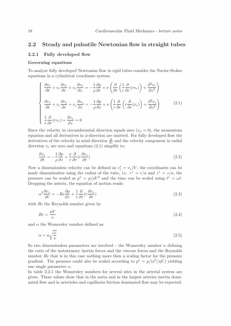
2.2.1 Fully developed flow
Governing equations
To analyze fully developed Newtonian flow in rigid tubes consider the Navier-Stokesequations in a cylindrical coordinate system:
∂vr∂t
+ vr∂vr∂r
+ vz∂vr∂z
= −1
ρ
∂p
∂r+ ν
(
∂
∂r
(
1
r
∂
∂r(rvr)
)
+∂2vr∂z2
)
∂vz∂t
+ vr∂vz∂r
+ vz∂vz∂z
= −1
ρ
∂p
∂z+ ν
(
1
r
∂
∂r
(
r∂
∂r(vz)
)
+∂2vz∂z2
)
1
r
∂
∂r(rvr) +
∂vz∂z
= 0
(2.1)
Since the velocity in circumferential direction equals zero (vφ = 0), the momentumequation and all derivatives in φ-direction are omitted. For fully developed flow thederivatives of the velocity in axial direction ∂
∂z and the velocity component in radialdirection vr are zero and equations (2.1) simplify to:
∂vz∂t
= −1
ρ
∂p
∂z+ν
r
∂
∂r(r∂vz∂r
) (2.2)
Now a dimensionless velocity can be defined as v∗z = vz/V , the coordinates can bemade dimensionless using the radius of the tube, i.e. r∗ = r/a and z∗ = z/a, thepressure can be scaled as p∗ = p/ρV 2 and the time can be scaled using t∗ = ωt.Dropping the asterix, the equation of motion reads:
α2 ∂vz∂t
= −Re∂p∂z
+1
r
∂
∂r(r∂vz∂r
) (2.3)
with Re the Reynolds number given by
Re =aV
ν(2.4)
and α the Womersley number defined as:
α = a
√
ω
ν(2.5)
So two dimensionless parameters are involved : the Womersley number α definingthe ratio of the instationary inertia forces and the viscous forces and the Reynoldsnumber Re that is in this case nothing more then a scaling factor for the pressuregradient. The pressure could also be scaled according to p∗ = p/(a2/ηV ) yieldingone single parameter α.In table 2.2.1 the Womersley numbers for several sites in the arterial system aregiven. These values show that in the aorta and in the largest arteries inertia domi-nated flow and in arterioles and capillaries friction dominated flow may be expected.
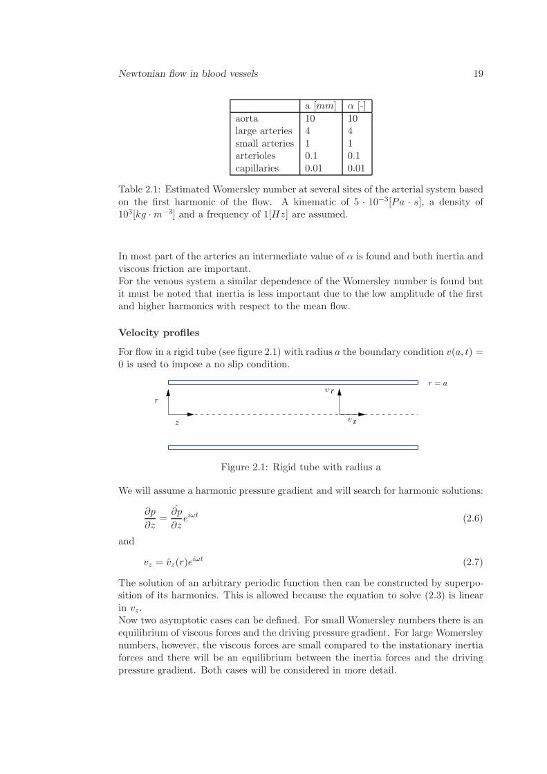
Newtonian flow in blood vessels 19
a [mm] α [-]
aorta 10 10large arteries 4 4small arteries 1 1arterioles 0.1 0.1capillaries 0.01 0.01
Table 2.1: Estimated Womersley number at several sites of the arterial system basedon the first harmonic of the flow. A kinematic of 5 · 10−3[Pa · s], a density of103[kg ·m−3] and a frequency of 1[Hz] are assumed.
In most part of the arteries an intermediate value of α is found and both inertia andviscous friction are important.For the venous system a similar dependence of the Womersley number is found butit must be noted that inertia is less important due to the low amplitude of the firstand higher harmonics with respect to the mean flow.
Velocity profiles
For flow in a rigid tube (see figure 2.1) with radius a the boundary condition v(a, t) =0 is used to impose a no slip condition.
r
zv
r
r = av
z
Figure 2.1: Rigid tube with radius a
We will assume a harmonic pressure gradient and will search for harmonic solutions:
∂p
∂z=∂p
∂zeiωt (2.6)
and
vz = vz(r)eiωt (2.7)
The solution of an arbitrary periodic function then can be constructed by superpo-sition of its harmonics. This is allowed because the equation to solve (2.3) is linearin vz.Now two asymptotic cases can be defined. For small Womersley numbers there is anequilibrium of viscous forces and the driving pressure gradient. For large Womersleynumbers, however, the viscous forces are small compared to the instationary inertiaforces and there will be an equilibrium between the inertia forces and the drivingpressure gradient. Both cases will be considered in more detail.
20 Cardiovascular Fluid Mechanics - lecture notes
Small Womersley number flow. If α ≪ 1 equation (2.3) (again in dimension-full form) yields:
0 = −1
ρ
∂p
∂z+ν
r
∂
∂r(r∂vz∂r
) (2.8)
Substitution of (2.6) and (2.7) yields:
ν∂2vz(r)
∂r2+ν
r
∂vz(r)
∂r=
1
ρ
∂p
∂z(2.9)
with solution:
vz(r, t) = − 1
4η
∂p
∂z(a2 − r2)eiωt (2.10)
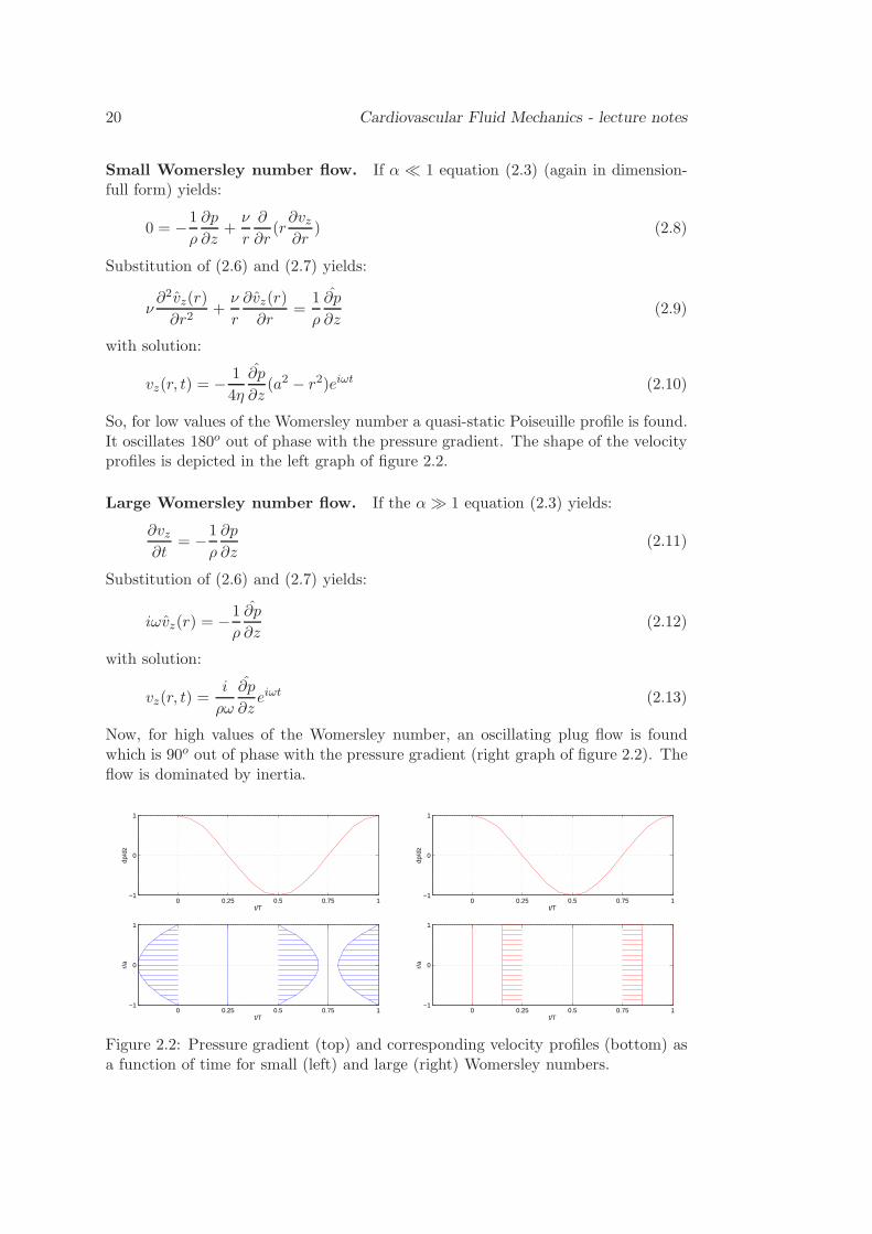
So, for low values of the Womersley number a quasi-static Poiseuille profile is found.It oscillates 180o out of phase with the pressure gradient. The shape of the velocityprofiles is depicted in the left graph of figure 2.2.
Large Womersley number flow. If the α≫ 1 equation (2.3) yields:
∂vz∂t
= −1
ρ
∂p
∂z(2.11)
Substitution of (2.6) and (2.7) yields:
iωvz(r) = −1
ρ
∂p
∂z(2.12)
with solution:
vz(r, t) =i
ρω
∂p
∂zeiωt (2.13)
Now, for high values of the Womersley number, an oscillating plug flow is foundwhich is 90o out of phase with the pressure gradient (right graph of figure 2.2). Theflow is dominated by inertia.
0 0.25 0.5 0.75 1−1
0
1
t/T
r/a
0 0.25 0.5 0.75 1−1
0
1
t/T
dp/d
z
0 0.25 0.5 0.75 1−1
0
1
t/T
r/a
0 0.25 0.5 0.75 1−1
0
1
t/T
dp/d
z
Figure 2.2: Pressure gradient (top) and corresponding velocity profiles (bottom) asa function of time for small (left) and large (right) Womersley numbers.
Newtonian flow in blood vessels 21
Arbitrary Womersley number flow. Substitution of (2.6) and (2.7) in equation(2.2) yields:
ν∂2vz(r)
∂r2+ν
r
∂vz(r)
∂r− iωvz(r) =
1
ρ
∂p
∂z(2.14)
Substitution of
s = i3/2αr/a (2.15)
in the homogeneous part of this equation yields the equation of Bessel for n = 0:
∂2vz∂s2
+1
s
∂vz∂s
+ (1− n2
s2)vz = 0 (2.16)
with solution given by the Bessel functions of the first kind:
Jn(s) =∞∑
k=0
(−1)k
k!(n + k)!
(
s
2
)2k+n
(2.17)
so:
J0(s) =∞∑
k=0
(−1)k
k!k!
(
s
2
)2k
= 1− (s
2)2 +
1
1222(z
2)4 − 1
122232(z
2)6 + ... (2.18)
(see Abramowitz and Stegun, 1964).
Together with the particular solution :
vpz =i
ρω
∂p
∂z(2.19)
we have:
vz(s) = KJ0(s) + vpz (2.20)
Using the boundary condition vz(a) = 0 then yields:
K = − vpzJ0(αi3/2)
(2.21)
and finally:
vz(r) =i
ρω
∂p
∂z
[
1− J0(i3/2αr/a)
J0(i3/2α)
]
(2.22)
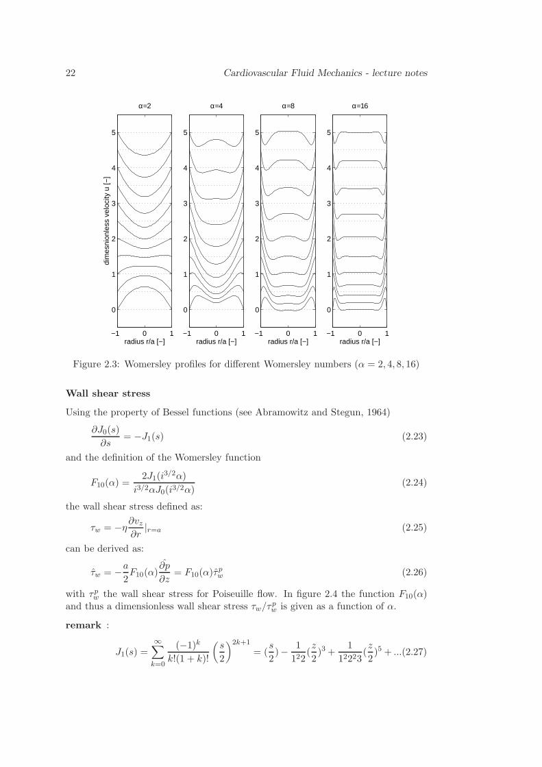
These are the well known Womersley profiles (Womersley, 1957) displayed in figure2.3. As can be seen from this figure, the Womersley profiles for intermediate Wom-ersley numbers are characterized by a phase-shift between the flow in the boundarylayer and the flow in the central core of the tube. Actually, in the boundary layerviscous forces dominate the inertia forces and the flow behaves like the flow for smallWomersley numbers. For high enough Womersley numbers, in the central core, in-ertia forces are dominant and flattened profiles that are shifted in phase are found.The thickness of the instationary boundary layer is determined by the Womersleynumber. This will be discussed in more detail in section 2.2.2.
22 Cardiovascular Fluid Mechanics - lecture notes
−1 0 1
0
1
2
3
4
5
dim
esni
onle
ss v
eloc
ity u
[−]
radius r/a [−]
α=2
−1 0 1
0
1
2
3
4
5
radius r/a [−]
α=4
−1 0 1
0
1
2
3
4
5
radius r/a [−]
α=8
−1 0 1
0
1
2
3
4
5
radius r/a [−]
α=16
Figure 2.3: Womersley profiles for different Womersley numbers (α = 2, 4, 8, 16)
Wall shear stress
Using the property of Bessel functions (see Abramowitz and Stegun, 1964)
∂J0(s)
∂s= −J1(s) (2.23)
and the definition of the Womersley function
F10(α) =2J1(i
3/2α)
i3/2αJ0(i3/2α)(2.24)
the wall shear stress defined as:
τw = −η∂vz∂r
|r=a (2.25)
can be derived as:
τw = −a2F10(α)
∂p
∂z= F10(α)τ
pw (2.26)
with τpw the wall shear stress for Poiseuille flow. In figure 2.4 the function F10(α)and thus a dimensionless wall shear stress τw/τ
pw is given as a function of α.
remark :
J1(s) =∞∑
k=0
(−1)k
k!(1 + k)!
(
s
2
)2k+1
= (s
2)− 1
122(z
2)3 +
1
12223(z
2)5 + ...(2.27)
Newtonian flow in blood vessels 23
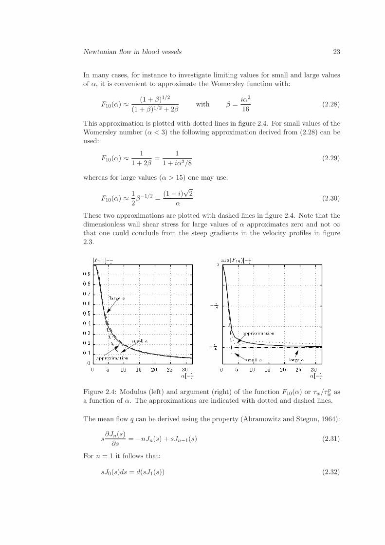
In many cases, for instance to investigate limiting values for small and large valuesof α, it is convenient to approximate the Womersley function with:
F10(α) ≈(1 + β)1/2
(1 + β)1/2 + 2βwith β =
iα2
16(2.28)
This approximation is plotted with dotted lines in figure 2.4. For small values of theWomersley number (α < 3) the following approximation derived from (2.28) can beused:
F10(α) ≈1
1 + 2β=
1
1 + iα2/8(2.29)
whereas for large values (α > 15) one may use:
F10(α) ≈1
2β−1/2 =
(1− i)√2
α(2.30)
These two approximations are plotted with dashed lines in figure 2.4. Note that thedimensionless wall shear stress for large values of α approximates zero and not ∞that one could conclude from the steep gradients in the velocity profiles in figure2.3.
00.10.20.30.40.50.60.70.8 jF10j[]0 5 10 15 20 25 30
0 arg(F10)[]0.9[]5 10 15 20 25 300 []48large approximation small approximationsmall large
Figure 2.4: Modulus (left) and argument (right) of the function F10(α) or τw/τpw as
a function of α. The approximations are indicated with dotted and dashed lines.
The mean flow q can be derived using the property (Abramowitz and Stegun, 1964):
s∂Jn(s)
∂s= −nJn(s) + sJn−1(s) (2.31)
For n = 1 it follows that:
sJ0(s)ds = d(sJ1(s)) (2.32)
24 Cardiovascular Fluid Mechanics - lecture notes
and together with J1(0) = 0 the flow becomes:
q =
a∫
0
vz2πrdr = iπa2
ρω[1− F10(α)]
∂p
∂z
= [1− F10(α)] q∞
=8i
α2[1− F10(α)] qp
(2.33)
with
q∞ =iπa2
ρω
∂p
∂zand qp =
πa4
8η
∂p
∂z(2.34)
Combining equation (2.26) with equation (2.33) by elimination of ∂p∂z finally yields:
τw =a
2Aiωρ
F10(α)
1− F10(α)q (2.35)
With A = πa2 the cross-sectional area of the tube. In the next chapter this expres-sion for the wall shear stress will be used to approximate the shear forces that thefluid exerts on the wall of the vessel.
Vascular impedance
The longitudinal impedance defined as:
ZL = − ∂p∂z/q (2.36)
can be derived directly from equation (2.33) and reads:
ZL = iωρ
πa21
1− F10(α)(2.37)
For a Poiseuille profile the longitudinal impedance is defined by integration of (2.10)and is given by:
Zp =8η
πa4(2.38)
From this it can be derived that the impedance of a rigid tube for oscillating flow re-lated to the impedance for steady flow (Poiseuille resistance) is given by the followingequation:
ZL
Zp=iα2
8
1
1− F10(α)(2.39)
In figure 2.5 the relative impedance is plotted as a function of the Womersley numberα. The relative longitudinal impedance is real for α ≪ 1 and becomes imaginaryfor α → ∞. This expresses the fact that for low frequencies (or small diameters)
Newtonian flow in blood vessels 25
modulus
real
imag
1 10 1000.1
1
10
100
1000
α
rela
tive
impe
danc
e
modulus
real
imag
0 8 16 24 320
20
40
60
80
100
α
real
tive
impe
danc
eargument
0 8 16 24 320
π/4
π/2
α
rela
tive
impe
danc
e
argument
1 10 100π/16
π/8
π/4
π/2
α
rela
tive
impe
danc
e
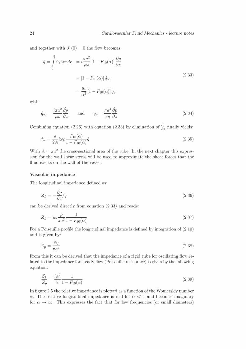
Figure 2.5: The relative impedance for oscillating flow in a tube (linear scale at thetop and logarithmic scale at the bottom) as a function of α.
the viscous forces are dominant, whereas for high frequencies (or large diameters)inertia is dominant and the flow behaves as an inviscid flow.
For small values of α the relative impedance results in (see 2.29):
ZL(α < 3)
Zp≈ 1 +
iα2
8(2.40)
Viscous forces then dominate and the pressure gradient is in phase with the flowand does not (strongly) depend on alpha. For large values of α (2.30) gives:
ZL(α > 15)
Zp≈ iα2
8(2.41)
indicating that the pressure gradient is out of phase with the flow and increasesquadratically with α.
2.2.2 Entrance flow
In general the flow in blood vessels is not fully developed. Due to transitions andbifurcations the velocity profile has to develop from a certain profile at the entranceof the tube (see figure 2.6).
In order to obtain an idea of the length needed for the flow to develop, the flow witha characteristic velocity V along a smooth boundary with characteristic length L is
26 Cardiovascular Fluid Mechanics - lecture notes
V
L
δ
x2
x1
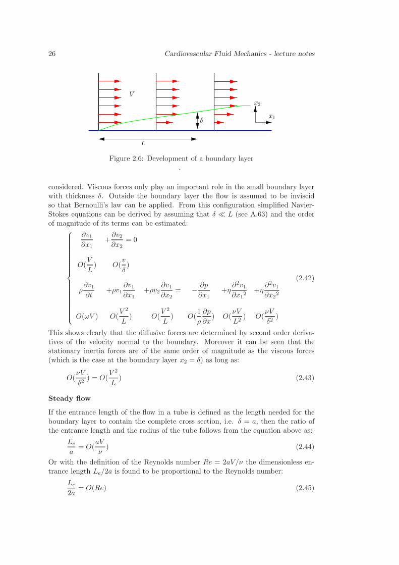
Figure 2.6: Development of a boundary layer.
considered. Viscous forces only play an important role in the small boundary layerwith thickness δ. Outside the boundary layer the flow is assumed to be inviscidso that Bernoulli’s law can be applied. From this configuration simplified Navier-Stokes equations can be derived by assuming that δ ≪ L (see A.63) and the orderof magnitude of its terms can be estimated:
∂v1∂x1
+∂v2∂x2
= 0
O(V
L) O(
v
δ)
ρ∂v1∂t
+ρv1∂v1∂x1
+ρv2∂v1∂x2
= − ∂p
∂x1+η
∂2v1∂x12
+η∂2v1∂x22
O(ωV ) O(V 2
L) O(
V 2
L) O(
1
ρ
∂p
∂x) O(
νV
L2) O(
νV
δ2)
(2.42)
This shows clearly that the diffusive forces are determined by second order deriva-tives of the velocity normal to the boundary. Moreover it can be seen that thestationary inertia forces are of the same order of magnitude as the viscous forces(which is the case at the boundary layer x2 = δ) as long as:
O(νV
δ2) = O(
V 2
L) (2.43)
Steady flow
If the entrance length of the flow in a tube is defined as the length needed for theboundary layer to contain the complete cross section, i.e. δ = a, then the ratio ofthe entrance length and the radius of the tube follows from the equation above as:
Le
a= O(
aV
ν) (2.44)
Or with the definition of the Reynolds number Re = 2aV/ν the dimensionless en-trance length Le/2a is found to be proportional to the Reynolds number:
Le
2a= O(Re) (2.45)
Newtonian flow in blood vessels 27
In Schlichting (1960) one can find that for laminar flow, for Le : v(Le, 0) = 0.99 ·2V :
Le
2a= 0.056Re (2.46)
For steady flow in the carotid artery, for instance, Re = 300, and thus Le ≈ 40a.This means that the flow will never become fully developed since the length of thecarotid artery is much less than 40 times its radius. In arterioles and smaller vessels,however, Re < 10 and hereby Le < a, so fully developed flow will be found in manycases.
Oscillating flow
For oscillating flow the inlet length is smaller as compared to the inlet length forsteady flow. This can be seen from the following. The unsteady inertia forces are ofthe same magnitude as the viscous forces when:
O(V ω) = O(νV
δ2) (2.47)
and thus:
δ = O(
√
ν
ω) (2.48)
This means that for fully developed oscillating flow a boundary layer exists with arelative thickness of:
δ
a= O(α−1) (2.49)
If, for oscillating flow, the inlet length is defined as the length for which the viscousforces still are of the same magnitude as the stationary inertia forces, i.e.:
O(νV
δ2) = O(
V 2
Le) (2.50)
then together with (2.49) the inlet length is of the order
Le = O(V δ2
ν) = O(
a
α2Re) (2.51)
Note that this holds only for α > 1. For α < 1 the boundary layer thicknessis restricted to the radius of the tube and we obtain an inlet length of the samemagnitude as for steady flow.
2.3 Steady and pulsating flow in curved and branched
tubes
2.3.1 Steady flow in a curved tube
Steady entrance flow in a curved tube
The flow in a curved tube is determined by an equilibrium of convective forces,pressure forces and viscous forces. Consider, the entrance flow in a curved tube
28 Cardiovascular Fluid Mechanics - lecture notes
inner wall lower wall
outer wall
upper wall
BCA
V
profilesaxial velocity
secondary velocitystreamlines
O
R0 θ
Rz
O
φ
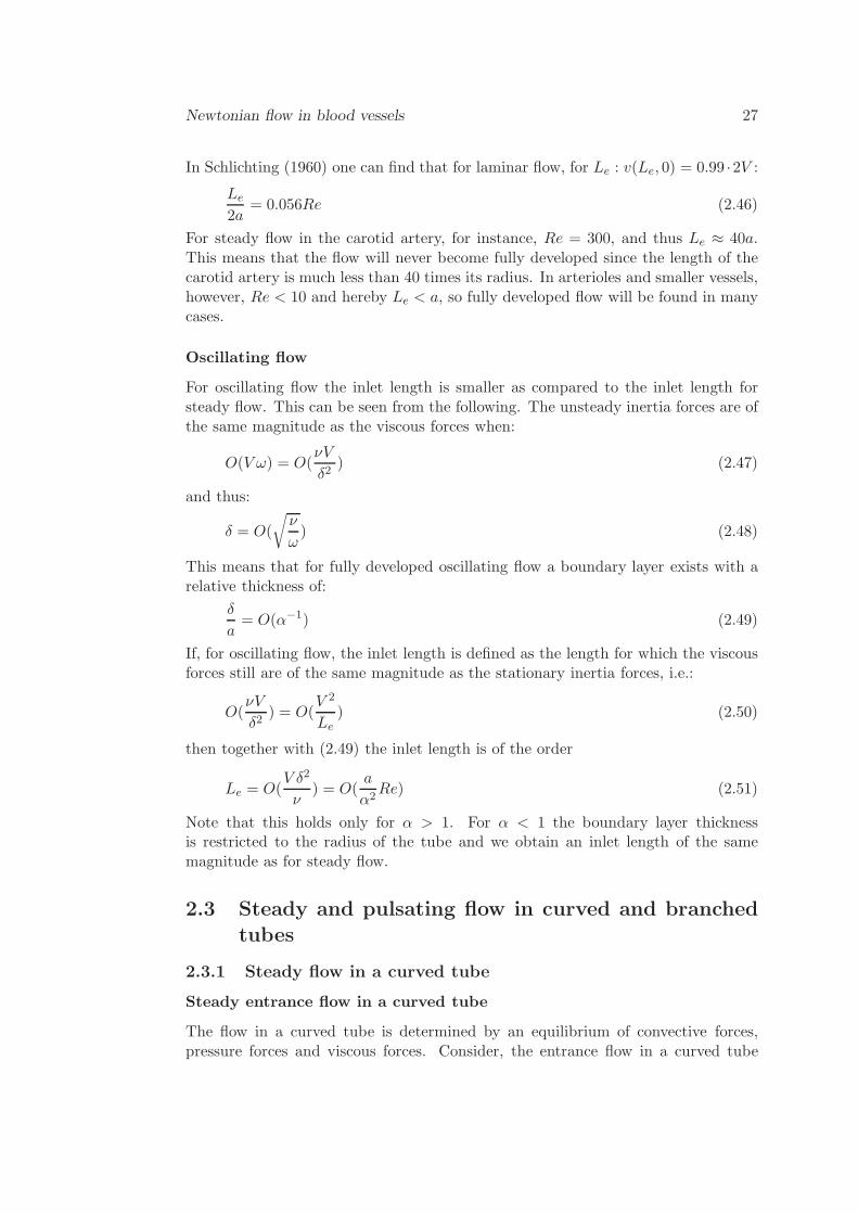
Figure 2.7: Axial velocity profiles, secondary velocity streamlines and helical motionof particles for entrance flow in a curved tube.
with radius a and a radius of curvature R0. With respect to the origin O we candefine a cylindrical coordinate system (R, z, φ). At the entrance (A: R0 − a < R <R0 + a, −a < z < a, φ = 0) a uniformly distributed irotational (plug) flow vφ = V(see figure 2.7) is assumed. As long as the boundary layer has not yet developed(R0φ << 0.1aRe) the viscous forces are restricted to a very thin boundary layer andthe velocity is restricted to one component, vφ. The other components (vR and vz)are small compared to vφ. In the core the flow is inviscid so Bernoulli’s law can beapplied:
p+ 12ρv
2φ = constant (2.52)
With p the pressure, and ρ the density of the fluid. The momentum equation inR-direction shows an equilibrium of pressure forces and centrifugal forces:
∂p
∂R=ρv2φR
(2.53)
As a consequence, the pressure is largest at the outer wall and smallest at the innerwall. Together with Bernoulli’s law it follows that the velocity will become largestat the inner wall and lowest at the outer wall of the tube (see figure 2.7 location(B)). Indeed, elimination of the pressure from (2.52) and (2.53) yields:
∂vφ∂R
= −vφR
(2.54)
and thus:
vφ =k1R
(2.55)
Newtonian flow in blood vessels 29
The constant k1 can be determined from the conservation of mass in the plane ofsymmetry (z = 0):
2aV =
R0+a∫
R0−a
vφ(R′)dR′ = k1 ln
R0 + a
R0 − a(2.56)
and thus:
k1 =2aV
ln 1+δ1−δ
(2.57)
with δ = a/R0. So in the entrance region (φ << 0.1δRe) initially the followingvelocity profile will develop:
vφ(R) =2aV
R ln 1+δ1−δ
(2.58)
It is easy to derive that for small values of δ this reduces to vφ(R) = (R0/R)V .Note that the velocity profile does only depend on R and does not depend on theazimuthal position θ in the tube. In terms of the toroidal coordinate system (r, θ, φ)we have:
R(r, θ) = R0 − r cos θ (2.59)
and the velocity profile given in (2.58) is:
vφ(r, θ) =2aV
(R0 − r cos θ) ln 1+δ1−δ
=2δV
(1− δ(r/a) cos θ) ln 1+δ1−δ
(2.60)
Again for small values of δ this reduces to vφ(r, θ) = V/(1− δ(r/a) cos θ).
Going more downstream, due to viscous forces a boundary layer will develop alongthe walls of the tube and will influence the complete velocity distribution. Finallythe velocity profile will look like the one that is sketched at position C. This profiledoes depend on the azimuthal position. In the plane of symmetry it will have amaximum that is shifted to the outer wall. In the direction perpendicular to theplane of symmetry an M-shaped profile will be found (see figure 2.7). This velocitydistribution can only be explained if we also consider the secondary flow field, i.e.the velocity components in the plane of a cross-section (φ =constant) of the tubeperpendicular to the axis.Viscous forces will diminish the axial velocity in the boundary layer along the wallof the curved tube. As a result, the equilibrium between the pressure gradient in R-direction and the centrifugal forces will be disturbed. In the boundary layers we will
have ρV 2
R < ∂p∂R and in the central core ρV 2
R > ∂p∂R . Consequently the fluid particles
in the central core will accelerate towards the outer wall, whereas fluid particles inthe boundary layer will accelerate in opposite direction. In this way a secondary
30 Cardiovascular Fluid Mechanics - lecture notes
vortex will develop as indicated in figure 2.7. This motion of fluid particles from theinner wall towards the outer wall in the core and along the upper and lower wallsback to the inner wall will have consequences for the axial velocity distribution.Particles with a relatively large axial velocity will move to the outer wall and due toconvective forces, the maximum of the axial velocity will shift in the same direction.On the other hand, particles in the boundary layer at the upper and lower walls willbe transported towards the inner wall and will convect a relatively low axial velocity.In this way in the plane of symmetry an axial velocity profile will develop with amaximum at the outer wall, and a minimum at the inner wall. For large curvaturesor large Reynolds numbers even negative axial velocity at the inner wall can occurdue to boundary layer separation.
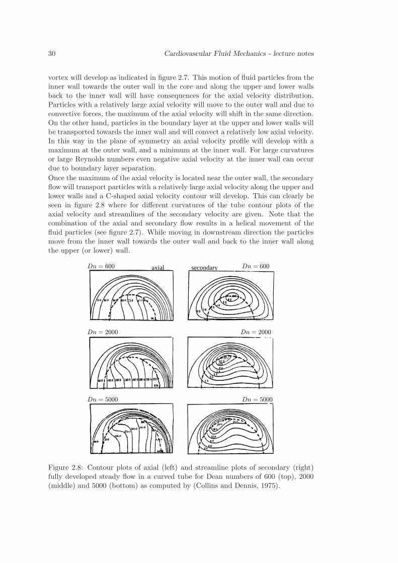
Once the maximum of the axial velocity is located near the outer wall, the secondaryflow will transport particles with a relatively large axial velocity along the upper andlower walls and a C-shaped axial velocity contour will develop. This can clearly beseen in figure 2.8 where for different curvatures of the tube contour plots of theaxial velocity and streamlines of the secondary velocity are given. Note that thecombination of the axial and secondary flow results in a helical movement of thefluid particles (see figure 2.7). While moving in downstream direction the particlesmove from the inner wall towards the outer wall and back to the inner wall alongthe upper (or lower) wall.
Dn = 5000 Dn = 5000
axialDn = 600 Dn = 600secondary
Dn = 2000 Dn = 2000
Figure 2.8: Contour plots of axial (left) and streamline plots of secondary (right)fully developed steady flow in a curved tube for Dean numbers of 600 (top), 2000(middle) and 5000 (bottom) as computed by (Collins and Dennis, 1975).
Newtonian flow in blood vessels 31
Steady fully developed flow in a curved tube
In order to obtain a more quantitative description of the flow phenomena it is conve-nient to use the toroidal coordinate system (r, θ, φ) as is depicted in figure 2.7. Thecorresponding velocity components are vr, vθ and vφ. The Navier-Stokes equationsin toroidal coordinates read (Ward-Smith, 1980):in r-direction:
∂vr∂t
+1
rB
[
∂
∂r(rBv2r) +
∂
∂θ(Bvrvθ) +
∂
∂φ(δrvφvr)−Bv2θ − δr cos θv2φ
]
=
−∂p∂r
+1
Re
1
rB
[
∂
∂r(rB
∂vr∂r
) +∂
∂θ(B
r
∂vr∂θ
) +∂
∂φ(δ2r
B
∂vr∂φ
)
]
−
1
r2(2∂vθ∂θ
+ vr) +δ sin θvθrB
+δ2 cos θ
B2(vθ sin θ − vr cos θ − 2
∂vφ∂φ
)
(2.61)
in θ-direction:
∂vθ∂t
+1
rB
[
∂
∂r(rBvrvθ) +
∂
∂θ(Bv2θ) +
∂
∂φ(δrvφvθ) +Bvrvθ + δr sin θv2φ
]
=
−∂p∂θ
+1
Re
1
rB
[
∂
∂r(rB
∂vθ∂r
) +∂
∂θ(B
r
∂vθ∂θ
) +∂
∂φ(δ2r
B
∂vθ∂φ
)
]
+
1
r2(2∂vr∂θ
− vθ)−δ sin θvrrB
− δ2 sin θ
B2(vθ sin θ − vr cos θ − 2
∂vφ∂φ
)
(2.62)
in φ-direction:
∂vφ∂t
+1
rB
[
∂
∂r(rBvφvr) +
∂
∂θ(Bvφvθ) +
∂
∂φ(δrv2φ) + δrvφ(vr cos θ − vθ sin θ)
]
=
− δ
B
∂p
∂φ+
1
Re
1
rB
[
∂
∂r(rB
∂vφ∂r
) +∂
∂θ(B
r
∂vφ∂θ
) +∂
∂φ(δ2r
B
∂vφ∂φ
)
]
+
2δ2
B2(∂vr∂φ
cos θ − ∂vθ∂φ
sin θ − vφ2)
(2.63)
continuity:
∂
∂r(rBvr) +
∂
∂θ(Bvθ) +
∂
∂φ(δrvφ) = 0 (2.64)
with
δ =a
R0and B = 1 + δr cos θ
For fully developed flow all derivatives in φ direction are zero ( ∂∂φ = 0). This of
course does not hold for the driving force ∂p∂φ . If we scale according to:
r∗ =r
a, p∗ =
p
ρV 2, v∗r =
vrV, v∗θ =
vθV, v∗φ =
vφV
(2.65)
32 Cardiovascular Fluid Mechanics - lecture notes
the continuity equation and the momentum equation in r-direction read after drop-ping the asterix:
∂vr∂r
+vrr
[
1 + 2δr cos θ
1 + δr cos θ
]
+1
r
∂vθ∂θ
− δvθ sin θ
1 + δr cos θ= 0 (2.66)
and
vr∂vr∂r
+vθr
∂vr∂θ
− v2θr
− δv2φ cos θ
1 + δr cos θ=
−∂p∂r
+1
Re
[(
1
r
∂
∂θ− δ sin θ
1 + δr cos θ
)(
1
r
∂vr∂θ
− ∂vθ∂r
− vθr
)]
(2.67)
The two important dimensionless parameters that appear are the curvature ratio δand the Reynolds number Re defined as:
δ =a
R0and Re =
2aV
ν(2.68)
with a the radius and R0 the curvature of the tube. If we restrict ourselves to theplane of symmetry (θ = 0, π , cos θ = ±1 and vθ = 0) we have for the momentumequation:
vr∂vr∂r
− δ±v2φ1± δr
= −∂p∂r
+1
Re
[(
1
r
∂
∂θ
)(
1
r
∂vr∂θ
− ∂vθ∂r
)]
(2.69)
If we consider small curvatures (δ ≪ 1) only, knowing that vφ = O(1) and r isalready scaled and in the interval [0, 1], the momentum equation yields vr
∂vr∂r =
O(δv2φ) = O(δ) and thus O(vr) = δ1/2. From the continuity equation (2.66) it canbe seen that vr and vθ scale in the same way, i.e. O(vr) = O(vθ), and thus alsoO(vθ) = δ1/2. If instead of using (2.65) we would use:
r∗ =r
a, p∗ =
p
δρV 2, v∗r =
vrδ1/2V
, v∗θ =vθ
δ1/2V, v∗φ =
vφV
(2.70)
The continuity equation and momentum equation in r-direction for δ ≪ 1 would be(again after dropping the asterix):
∂vr∂r
+vrr
+1
r
∂vθ∂θ
= 0 (2.71)
and
vr∂vr∂r
+vθr
∂vr∂θ
− v2θr
− v2φ cos θ =
−∂p∂r
+1
δ1/2Re
[
1
r
∂
∂θ
(
1
r
∂vr∂θ
− ∂vθ∂r
− vθr
)]
(2.72)
From this we can see that for small curvature another dimensionless parameter, theDean number, can be defined as:
Dn = δ1/2Re. (2.73)
Newtonian flow in blood vessels 33
The secondary flow depends on two important parameters, the Reynolds numberRe and the curvature δ or the Dean number Dn and the curvature δ. The lastcombination is often used because for small curvature only the Dean number is ofimportance.
For large Dean numbers the viscous term in (2.72) can be neglected in the core ofthe secondary flow field and one can talk about a boundary layer of the secondaryflow. The thickness δs of this boundary layer can be derived from the momentumequation in θ-direction:
vr∂vθ∂r
+vθr
∂vθ∂θ
− vrvθr
+ δv2φ sin θ
1 + δr cos θ=
−1
r
∂p
∂θ+
1
δ1/2Re
[(
∂
∂r+
δ cos θ
1 + δr cos θ
)(
∂vθ∂r
+vθr
− 1
r
∂vr∂r
)]
(2.74)
If we assume that at r = a− δs the viscous and inertia forces are of the same orderof magnitude we have:
δsa
= O(Dn−1/2) (2.75)
In figure 2.8 the boundary layer of the secondary flow is indicated with a dashedline and indeed decreases with increasing Dean numbers.
2.3.2 Unsteady fully developed flow in a curved tube
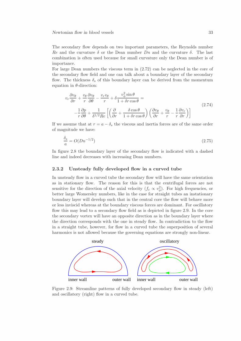
In unsteady flow in a curved tube the secondary flow will have the same orientationas in stationary flow. The reason for this is that the centrifugal forces are notsensitive for the direction of the axial velocity (fc ∝ v2φ). For high frequencies, orbetter large Womersley numbers, like in the case for straight tubes an instationaryboundary layer will develop such that in the central core the flow will behave moreor less inviscid whereas at the boundary viscous forces are dominant. For oscillatoryflow this may lead to a secondary flow field as is depicted in figure 2.9. In the corethe secondary vortex will have an opposite direction as in the boundary layer wherethe direction corresponds with the one in steady flow. In contradiction to the flowin a straight tube, however, for flow in a curved tube the superposition of severalharmonics is not allowed because the governing equations are strongly non-linear.
inner wall outer wall inner wall outer wall
oscillatorysteady
Figure 2.9: Streamline patterns of fully developed secondary flow in steady (left)and oscillatory (right) flow in a curved tube.
34 Cardiovascular Fluid Mechanics - lecture notes
0 0.1 0.2 0.3 0.4 0.5 0.6 0.7 0.8 0.9 10
0.2
0.4
0.6
0.8
1
1.2
1.4
exp.
4530
A A'A'
0 15 75
num.num.exp.
ooo: experimental |: numerical
exp.60 90
num.exp. num.BA A'AA'B'A
B B'
0 0.1 0.2 0.3 0.4 0.5 0.6 0.7 0.8 0.9 10
0.2
0.4
0.6
0.8
1
1.2
1.4
A A'B B' AA'B|: numerical
B'AA A'
A'0 15 30
exp.
45 60 75 90num.exp. num.exp.num.num.exp.
ooo: experimental
0 0.1 0.2 0.3 0.4 0.5 0.6 0.7 0.8 0.9 10
0.2
0.4
0.6
0.8
1
1.2
1.4
A A'B B' AA'B
exp.B'AA A'
A'0 15 30
ooo: experimental
exp.
|: numerical45 60 75 90
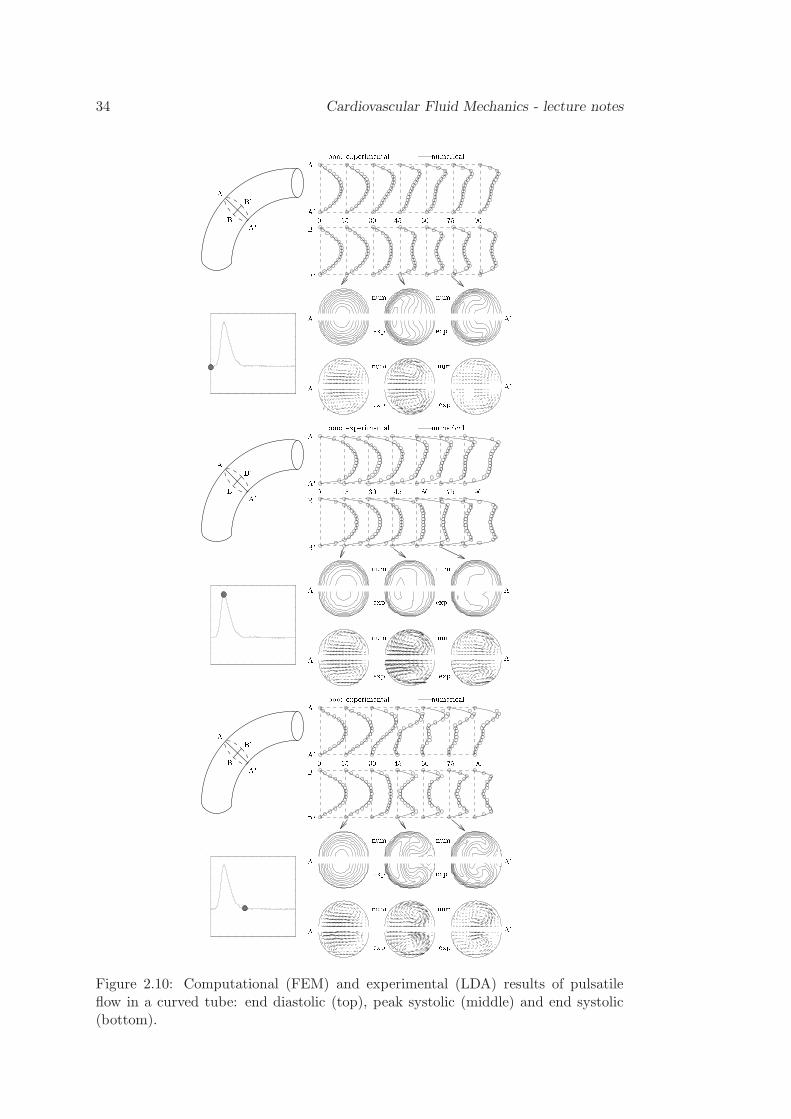
num.exp. num.exp.num.num.Figure 2.10: Computational (FEM) and experimental (LDA) results of pulsatileflow in a curved tube: end diastolic (top), peak systolic (middle) and end systolic(bottom).
Newtonian flow in blood vessels 35
In pulsating flow this second vortex will not be that pronounced as in oscillatingflow but some influence can be depicted. This is shown in the figure 2.10 where theresults of a finite element computation of pulsating flow in a curved tube are giventogether with experimental (laser Doppler) data.
2.3.3 Flow in branched tubes
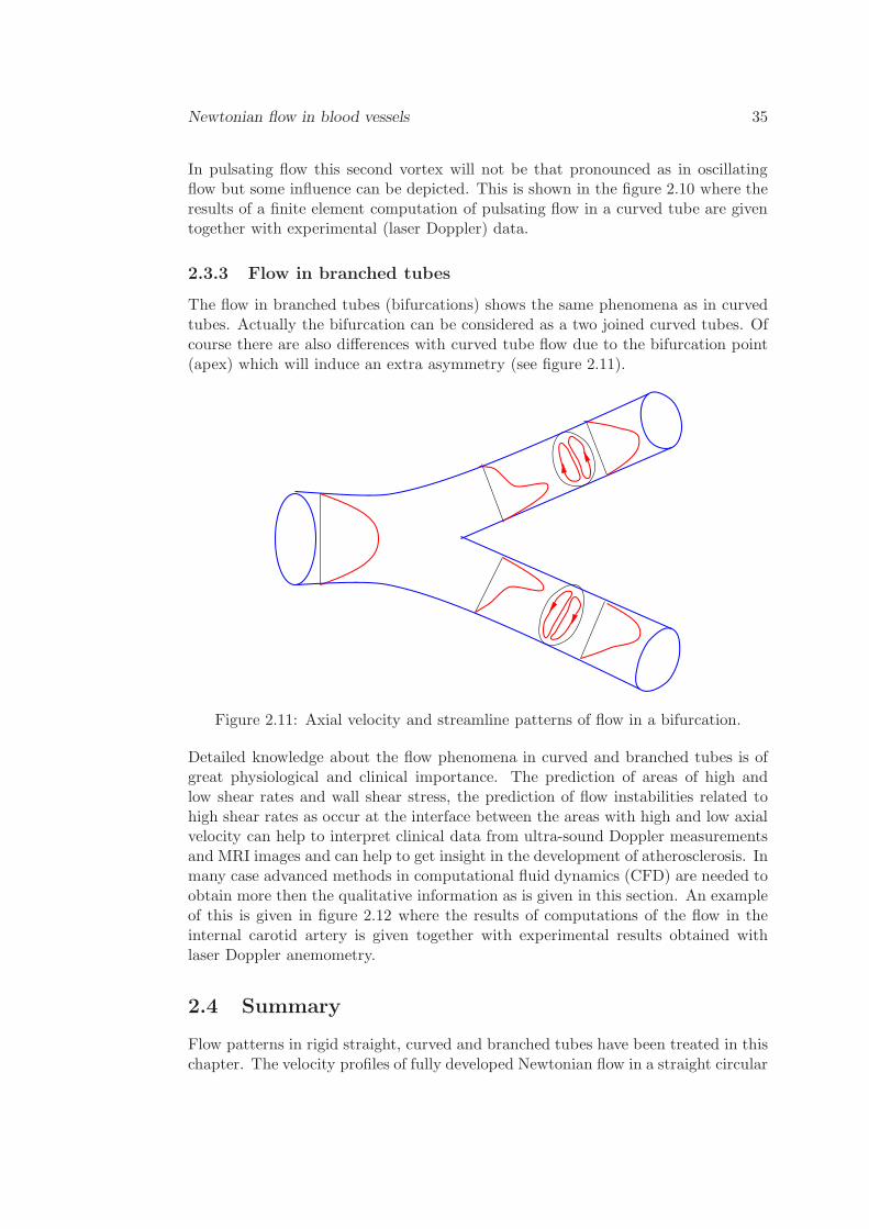
The flow in branched tubes (bifurcations) shows the same phenomena as in curvedtubes. Actually the bifurcation can be considered as a two joined curved tubes. Ofcourse there are also differences with curved tube flow due to the bifurcation point(apex) which will induce an extra asymmetry (see figure 2.11).
Figure 2.11: Axial velocity and streamline patterns of flow in a bifurcation.
Detailed knowledge about the flow phenomena in curved and branched tubes is ofgreat physiological and clinical importance. The prediction of areas of high andlow shear rates and wall shear stress, the prediction of flow instabilities related tohigh shear rates as occur at the interface between the areas with high and low axialvelocity can help to interpret clinical data from ultra-sound Doppler measurementsand MRI images and can help to get insight in the development of atherosclerosis. Inmany case advanced methods in computational fluid dynamics (CFD) are needed toobtain more then the qualitative information as is given in this section. An exampleof this is given in figure 2.12 where the results of computations of the flow in theinternal carotid artery is given together with experimental results obtained withlaser Doppler anemometry.
2.4 Summary
Flow patterns in rigid straight, curved and branched tubes have been treated in thischapter. The velocity profiles of fully developed Newtonian flow in a straight circular
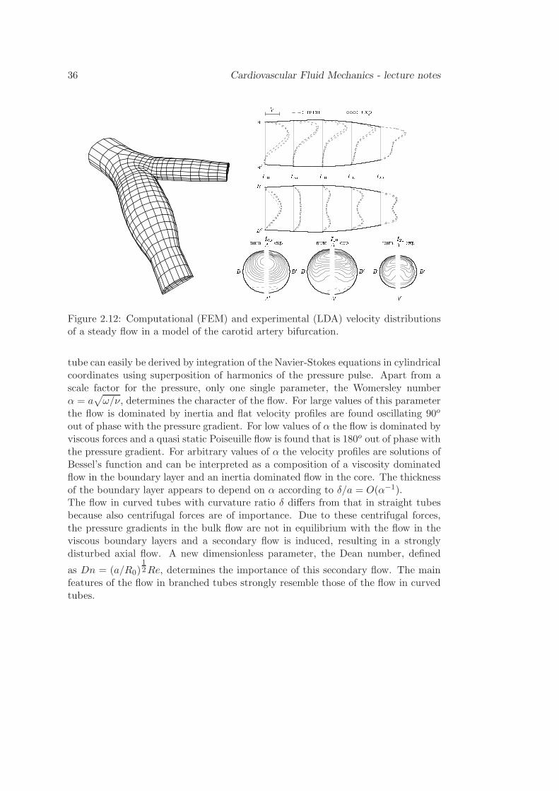
36 Cardiovascular Fluid Mechanics - lecture notes: num. : exp.I05I00 I10 I15 I20
AA0
exp.BB0
V
A A AB BA0 A0 A0B B0 B0 B0I00 I10 I20num. exp. num. exp. num.Figure 2.12: Computational (FEM) and experimental (LDA) velocity distributionsof a steady flow in a model of the carotid artery bifurcation.
tube can easily be derived by integration of the Navier-Stokes equations in cylindricalcoordinates using superposition of harmonics of the pressure pulse. Apart from ascale factor for the pressure, only one single parameter, the Womersley numberα = a
√
ω/ν, determines the character of the flow. For large values of this parameterthe flow is dominated by inertia and flat velocity profiles are found oscillating 90o
out of phase with the pressure gradient. For low values of α the flow is dominated byviscous forces and a quasi static Poiseuille flow is found that is 180o out of phase withthe pressure gradient. For arbitrary values of α the velocity profiles are solutions ofBessel’s function and can be interpreted as a composition of a viscosity dominatedflow in the boundary layer and an inertia dominated flow in the core. The thicknessof the boundary layer appears to depend on α according to δ/a = O(α−1).The flow in curved tubes with curvature ratio δ differs from that in straight tubesbecause also centrifugal forces are of importance. Due to these centrifugal forces,the pressure gradients in the bulk flow are not in equilibrium with the flow in theviscous boundary layers and a secondary flow is induced, resulting in a stronglydisturbed axial flow. A new dimensionless parameter, the Dean number, defined
as Dn = (a/R0)12Re, determines the importance of this secondary flow. The main
features of the flow in branched tubes strongly resemble those of the flow in curvedtubes.
Chapter 3
Mechanics of the vessel wall
3.1 Introduction
In the arterial system, the amplitude of the pressure pulse is that large that the ar-teries significantly deform during the cardiac cycle. This deformation is determinedby the mechanical properties of the arterial wall. In this section an outline of themechanical properties of the main constituents of the vessel wall and the wall as awhole is given taking the morphology as a point of departure. A simple linear elasticmodel for wall displacement due to change in transmural pressure will be derived.
37
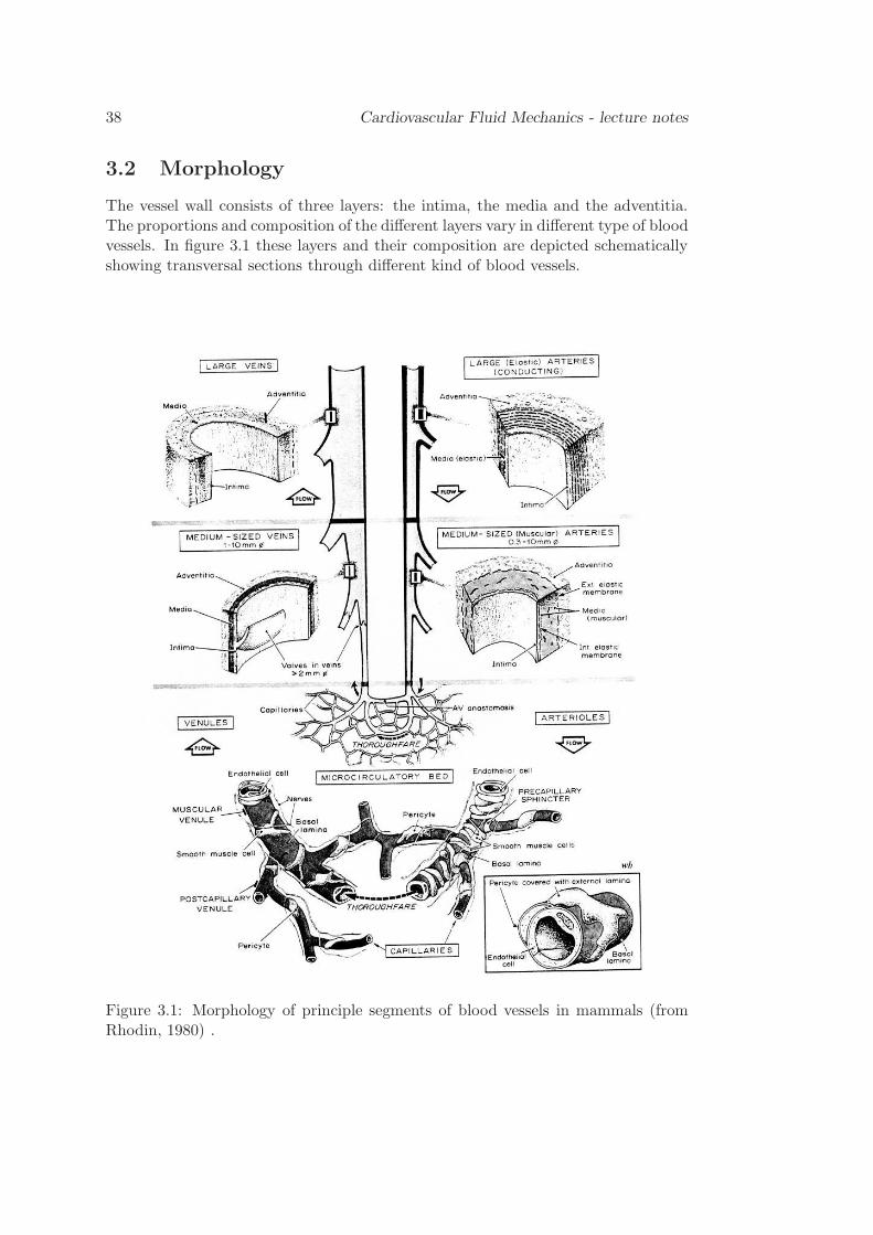
38 Cardiovascular Fluid Mechanics - lecture notes
3.2 Morphology
The vessel wall consists of three layers: the intima, the media and the adventitia.The proportions and composition of the different layers vary in different type of bloodvessels. In figure 3.1 these layers and their composition are depicted schematicallyshowing transversal sections through different kind of blood vessels.
Figure 3.1: Morphology of principle segments of blood vessels in mammals (fromRhodin, 1980) .
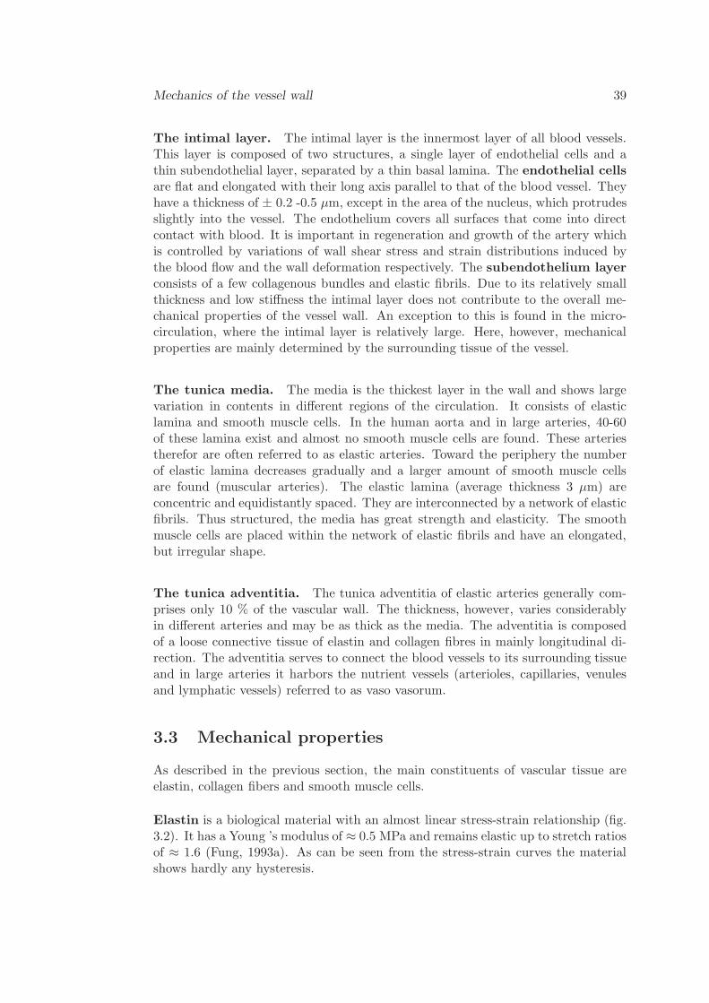
Mechanics of the vessel wall 39
The intimal layer. The intimal layer is the innermost layer of all blood vessels.This layer is composed of two structures, a single layer of endothelial cells and athin subendothelial layer, separated by a thin basal lamina. The endothelial cellsare flat and elongated with their long axis parallel to that of the blood vessel. Theyhave a thickness of ± 0.2 -0.5 µm, except in the area of the nucleus, which protrudesslightly into the vessel. The endothelium covers all surfaces that come into directcontact with blood. It is important in regeneration and growth of the artery whichis controlled by variations of wall shear stress and strain distributions induced bythe blood flow and the wall deformation respectively. The subendothelium layer
consists of a few collagenous bundles and elastic fibrils. Due to its relatively smallthickness and low stiffness the intimal layer does not contribute to the overall me-chanical properties of the vessel wall. An exception to this is found in the micro-circulation, where the intimal layer is relatively large. Here, however, mechanicalproperties are mainly determined by the surrounding tissue of the vessel.
The tunica media. The media is the thickest layer in the wall and shows largevariation in contents in different regions of the circulation. It consists of elasticlamina and smooth muscle cells. In the human aorta and in large arteries, 40-60of these lamina exist and almost no smooth muscle cells are found. These arteriestherefor are often referred to as elastic arteries. Toward the periphery the numberof elastic lamina decreases gradually and a larger amount of smooth muscle cellsare found (muscular arteries). The elastic lamina (average thickness 3 µm) areconcentric and equidistantly spaced. They are interconnected by a network of elasticfibrils. Thus structured, the media has great strength and elasticity. The smoothmuscle cells are placed within the network of elastic fibrils and have an elongated,but irregular shape.
The tunica adventitia. The tunica adventitia of elastic arteries generally com-prises only 10 % of the vascular wall. The thickness, however, varies considerablyin different arteries and may be as thick as the media. The adventitia is composedof a loose connective tissue of elastin and collagen fibres in mainly longitudinal di-rection. The adventitia serves to connect the blood vessels to its surrounding tissueand in large arteries it harbors the nutrient vessels (arterioles, capillaries, venulesand lymphatic vessels) referred to as vaso vasorum.
3.3 Mechanical properties
As described in the previous section, the main constituents of vascular tissue areelastin, collagen fibers and smooth muscle cells.
Elastin is a biological material with an almost linear stress-strain relationship (fig.3.2). It has a Young ’s modulus of ≈ 0.5 MPa and remains elastic up to stretch ratiosof ≈ 1.6 (Fung, 1993a). As can be seen from the stress-strain curves the materialshows hardly any hysteresis.
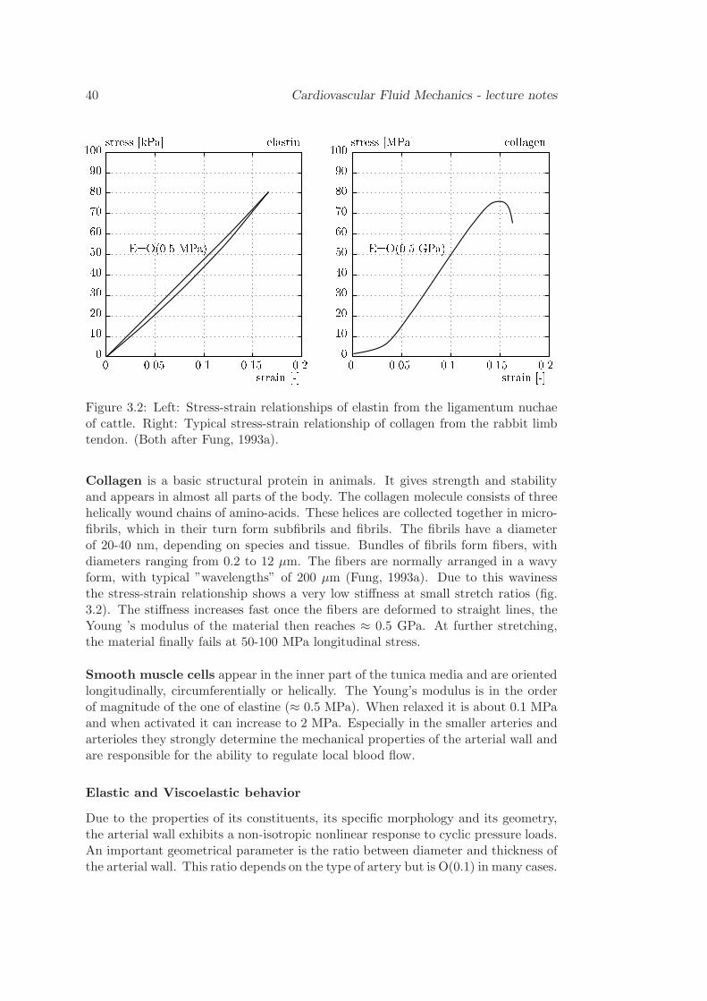
40 Cardiovascular Fluid Mechanics - lecture notes
0.05 0.1 0.15 0.20102030405060708090100
strain [-]
stress [kPa] elastin
0 0.05 0.1 0.15 0.20102030405060708090100
strain [-]
stress [MPa] collagen
0E=O(0.5 MPa) E=O(0.5 GPa)
Figure 3.2: Left: Stress-strain relationships of elastin from the ligamentum nuchaeof cattle. Right: Typical stress-strain relationship of collagen from the rabbit limbtendon. (Both after Fung, 1993a).
Collagen is a basic structural protein in animals. It gives strength and stabilityand appears in almost all parts of the body. The collagen molecule consists of threehelically wound chains of amino-acids. These helices are collected together in micro-fibrils, which in their turn form subfibrils and fibrils. The fibrils have a diameterof 20-40 nm, depending on species and tissue. Bundles of fibrils form fibers, withdiameters ranging from 0.2 to 12 µm. The fibers are normally arranged in a wavyform, with typical ”wavelengths” of 200 µm (Fung, 1993a). Due to this wavinessthe stress-strain relationship shows a very low stiffness at small stretch ratios (fig.3.2). The stiffness increases fast once the fibers are deformed to straight lines, theYoung ’s modulus of the material then reaches ≈ 0.5 GPa. At further stretching,the material finally fails at 50-100 MPa longitudinal stress.
Smooth muscle cells appear in the inner part of the tunica media and are orientedlongitudinally, circumferentially or helically. The Young’s modulus is in the orderof magnitude of the one of elastine (≈ 0.5 MPa). When relaxed it is about 0.1 MPaand when activated it can increase to 2 MPa. Especially in the smaller arteries andarterioles they strongly determine the mechanical properties of the arterial wall andare responsible for the ability to regulate local blood flow.
Elastic and Viscoelastic behavior
Due to the properties of its constituents, its specific morphology and its geometry,the arterial wall exhibits a non-isotropic nonlinear response to cyclic pressure loads.An important geometrical parameter is the ratio between diameter and thickness ofthe arterial wall. This ratio depends on the type of artery but is O(0.1) in many cases.
Mechanics of the vessel wall 41
Moreover the vessels are thetered mainly longitudinal by the surrounding tissue. Dueto these complex properties it formally is not possible to define a Young’s modulusas can be done in linear elasticity theory. Still in order to obtain a global idea ofthe elastic behavior it is possible to lump all properties together as if the vessel wallwas homogeneous. This can be done by measuring the stress strain relationship anduse the result to define an effective Young’s modulus. In figure 3.3 a typical stressstrain relationship of a large artery is shown. The stiffness in longitudinal directionis higher then in circumferential direction especially at larger stretch ratios yieldinga different effective incremental Young’s modulus. Still the relation is non-linear dueto the wavy form of the collagen fibres that consequently contribute to the stiffnessonly at higher stretch ratios. It will be clear that linear elasticity can not be appliedstraight forward. Linearization, however, about an equilibrium state (for instancethe mean or diastolic pressure) yields a linearized or incremantal effective Young’smodulus that in many cases is approriate the use in linear elasticity analysis.
longitudinalcircumferantial1 1.1 1.2 1.3 1.4 1.5 1.6 1.700.10.20.30.40.50.60.70.80.9
stretch ratio [-]
Cauchy stress [MPa]
Figure 3.3: Typical stress-strain relationship (broken line = longitudinal, solid line= circumferential) of aortic wall material (after Kasyanov and Knet-s, 1974) .
Vascular tissue normally is viscoelastic. When a cyclic load is applied to it inan experiment, the load-displacement curve for loading differs from the unloadingcurve: hysteresis due to viscoelasticity is found ( see figure 3.2). Moreover, thecurves change after several repetitions of the same loading/unloading cycle. After acertain number of repetitions, the loading-unloading curve doesn’t change anymore,and the loading/unloading curves almost coincide. The state of the specimen then iscalled preconditioned (Fung et al., 1979; Fung, 1993a). How well this state resembles
42 Cardiovascular Fluid Mechanics - lecture notes
the in-vivo situation is not reported.
3.4 Incompressible elastic deformation
In appendix A section A.2.4 it is shown that in general elastic solids can be describedby the constitutive equation σ = −pI + τ (B). The most simple version of such arelation will be the one in which the extra stress τ linearly depends on the Fingertensor. Materials that obey such a relation are referred to as linear elastic or neo-Hookean solids. Most rubber like materials but also to some extend biologicaltissues like the arterial wall are reasonably described by such a neo-Hookean model.
3.4.1 Deformation of incompressible linear elastic solids
The equations that describe the deformation of incompressible linear elastic solidsare given by the continuity equation (A.38) and the momentum equation (A.39)together with the constitutive equation:
σ = −pI +G(B − I) (3.1)
with p the pressure and G the shear modulus. Note that the linear relation betweenthe extra stress and the strain is taken such that if there is no deformation (B = I)the strain measure B− I = 0. The momentum and continuity equations then read:
ρ∂v
∂t+ ρ(v · ∇)v = ρf −∇p+G∇ · (B − I).
∇ · v = 0
(3.2)
After introduction of the non-dimensional variables x∗ = x/L, t∗ = t/θ and char-acteristic strain γ, the characteristic displacement is U = γL and the characteris-tic velocity is V = U/θ = γL/θ. Using a characteristic pressure p∗ = p/p0, thedimensionless equations for elastic deformation then become (after dropping thesuperscript ∗):
ργL
θ2∂v
∂t+ργ2L
θ2(v · ∇)v = ρgf − p0
L∇p+ γG
L∇ · (B − I)
∇ · v = 0
(3.3)
Unfortunately in the solid mechanics community it is not common to use dimen-sionless parameters and we have to introduce them ourselves or use an example toshow which of the terms are of importance in this equation. If we assume that wedeform a solid with density ρ = O(103)[kg/m3], shear modulus G = O(105)[Pa]and characteristic length L = O(10−2)[m] with a typical strain γ = O(10−1) in acharacteristic time θ = O(1)[s], the terms at the left hand side have an order ofmagnitude of O(1)[Pa/m] and O(10−2)[Pa/m]. The deformation forces at the righthand side, however, have an order of magnitude O(104)[Pa/m]. As a consequencethe terms at the left hand side can be neglected. Gravity forces can not be neglectedautomatically but are often not taken into account because they work on the body
Mechanics of the vessel wall 43
as a whole and do not induce extra deformation unless large hydrostatic pressuregradients occur. The momentum equation then reads:
∇ · σ = −∇p+G∇ · (B − I) = 0
det(F ) = 1(3.4)
Note that the continuity equation is expressed in terms of the deformation tensorF (see below). Equations (3.4) can be solved after applying boundary conditions ofthe form (see (A.43)):
in normal direction:prescribed displacement:
(u · n) = unΓ
or prescribed stress:(σ · n) · n = (s · n)
in tangential directions:prescribed displacemnet:
(u · ti) = utiΓ i = 1, 2
or prescribed stress:(σ · n) · ti = (s · ti)
(3.5)
In linear elasticity the incompressibility constraint (det(F ) = 1) is oftenly circum-vented by assuming the material to be (slightly) compressible. In that case it isconvenient to decompose the deformation in a volumetric part and an isochoric partaccording to:
F = J1/3F (3.6)
with J the volume ratio defined by:
J = det(F ) =dV
dV0(3.7)
Consequently det(F ) = det(J−1/3I) · det(F ) = 1 and an equivalent neo-Hookeanmodel can be taken according to:
σ = κ(J − 1)I +G(B − I) (3.8)
with κ the compression modulus and B = F · F c= J−2/3F · F c.
3.4.2 Approximation for small strains
For small strains γ (i.e. ||∇u|| ≈ ||∇0u|| << 1) the deformation tensor F can bewritten as:
F = (∇0x)c = (∇0(x0 + u))c = I + (∇0u)c ≈ I + (∇u)c (3.9)
The volume ratio for small deformations then yields:
J = det(F ) ≈ det(I + (∇u)c) ≈ 1 + tr(∇u) (3.10)
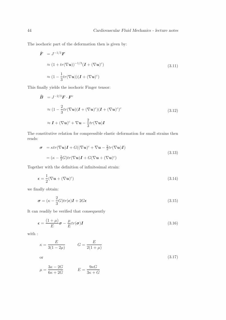
44 Cardiovascular Fluid Mechanics - lecture notes
The isochoric part of the deformation then is given by:
F = J−1/3F
≈ (1 + tr(∇u))−1/3(I + (∇u)c)
≈ (1− 1
3tr(∇u))(I + (∇u)c)
(3.11)
This finally yields the isochoric Finger tensor:
B = J−2/3F · F c
≈ (1− 2
3tr(∇u)(I + (∇u)c)(I + (∇u)c)c
≈ I + (∇u)c +∇u− 2
3tr(∇u)I
(3.12)
The constitutive relation for compressible elastic deformation for small strains thenreads:
σ = κtr(∇u)I +G((∇u)c +∇u− 23tr(∇u)I)
= (κ− 23G)tr(∇u)I +G(∇u+ (∇u)c)
(3.13)
Together with the definition of infinitesimal strain:
ǫ =1
2(∇u+ (∇u)c) (3.14)
we finally obtain:
σ = (κ− 2
3G)tr(ǫ)I + 2Gǫ (3.15)
It can readily be verified that consequently
ǫ =(1 + µ)
Eσ − µ
Etr(σ)I (3.16)
with :
κ =E
3(1 − 2µ)G =
E
2(1 + µ)
or
µ =3κ− 2G
6κ+ 2GE =
9κG
3κ+G
(3.17)
Mechanics of the vessel wall 45
Note that the Young’s modulus E and Poisson ratio µ can be determined by atensile test. Using the expression for the strain given by (3.16) it follows that:
ǫzz =∆l
l0=
1
Eσzz
ǫxx = ǫyy =∆h
h0= − µ
Eσzz
and consequently:
E =σzzǫzz
µ = −ǫxxǫzz
h0 h0 +hl0 +ll0
zz3.5 Wall motion
Consider a linear elastic thin walled tube with constant wall thickness h , densityρw, Young’s modulus E and Poisson’s ratio µ (see figure 3.4).
z
r
u
r=ah
r
v z
v
r
o
Figure 3.4: Distensible tube with radius a(z, t), wall thickness h
If the thickness of the wall is assumed to be that small that σrr = 0, the momentumequation in z-direction is given by:
εzz =∂uz∂z
=1
E(σzz − µσφφ) (3.18)
with uz the wall displacement in axial direction. Assuming again axial restraint(uz = 0) then εzz = 0 and thus:
σzz = µσφφ (3.19)
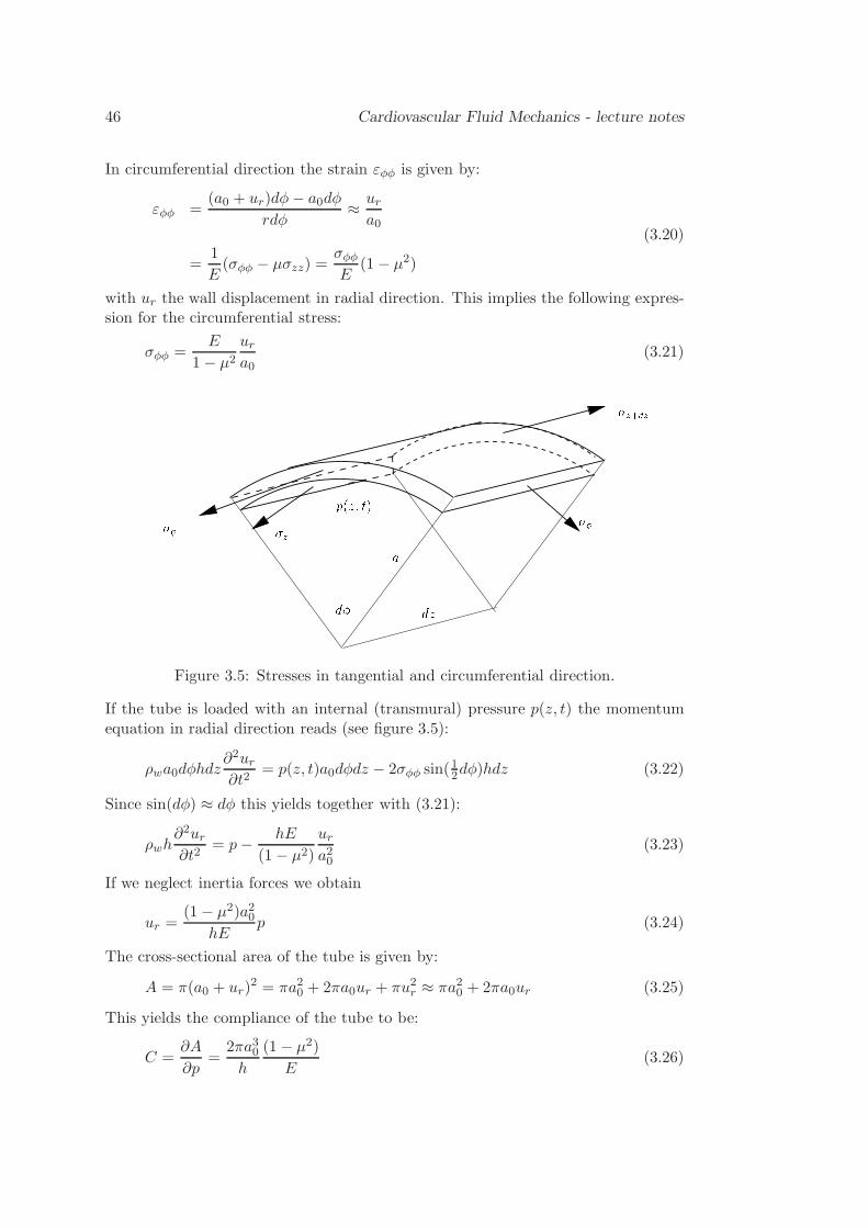
46 Cardiovascular Fluid Mechanics - lecture notes
In circumferential direction the strain εφφ is given by:
εφφ =(a0 + ur)dφ− a0dφ
rdφ≈ ura0
=1
E(σφφ − µσzz) =
σφφE
(1− µ2)
(3.20)
with ur the wall displacement in radial direction. This implies the following expres-sion for the circumferential stress:
σφφ =E
1− µ2ura0
(3.21)z+dzz p(z; t) ad dz
Figure 3.5: Stresses in tangential and circumferential direction.
If the tube is loaded with an internal (transmural) pressure p(z, t) the momentumequation in radial direction reads (see figure 3.5):
ρwa0dφhdz∂2ur∂t2
= p(z, t)a0dφdz − 2σφφ sin(12dφ)hdz (3.22)
Since sin(dφ) ≈ dφ this yields together with (3.21):
ρwh∂2ur∂t2
= p− hE
(1− µ2)
ura20
(3.23)
If we neglect inertia forces we obtain
ur =(1− µ2)a20
hEp (3.24)
The cross-sectional area of the tube is given by:
A = π(a0 + ur)2 = πa20 + 2πa0ur + πu2r ≈ πa20 + 2πa0ur (3.25)
This yields the compliance of the tube to be:
C =∂A
∂p=
2πa30h
(1− µ2)
E(3.26)
Mechanics of the vessel wall 47
Oftenly instead of the compliance C the distensibility
D =1
A0C =
2a0h
(1− µ2)
E(3.27)
is used. In the next chapter D will be used to derive expressions for the propagationof pressure waves in distensible tubes.
3.6 Summary
A short introduction to vessel wall mechanics based on morphology and materialproperties of the main constitutents (elastine and collagen) is given. Although theconstitutive behavior of vessel wall is anisotropic and visco-elastic simple linearelastic models based on thin walled tubes can be valuable. To this end, simpleexpressions for the compliance and distensibility of thin walled tubes are derivedand related to parameters that can be derived from tensile tests.

48 Cardiovascular Fluid Mechanics - lecture notes
Chapter 4
Wave phenomena in blood
vessels
4.1 Introduction
In this chapter we will show that traveling pressure and flow waves are the result ofthe distensibility (or compliance) of the arteries (see chapter 1 equations (1.2),(1.3)and (1.4) or chapter 3 equations (3.26) and (3.27)) and the pulsatile character ofthe pressure. A typical relation between the pressure and cross-sectional area of anartery is given in figure 1.7 and shows that the compliance normally does not have aconstant value but strongly depends on the pressure. In this chapter, however, onlysmall area variations will be considered and a linear relation between the pressureamplitude and the vessel diameter will be assumed. Apart from wave propagationand the importance of viscous forces expressed in the value of the Womersley numberα, also wave reflection from arterial bifurcations or transitions in mechanical orgeometrical properties will be dealt with. Moreover, attenuation of waves as a resultof fluid viscosity and wall visco-elasticity will be discussed.
49
50 Cardiovascular Fluid Mechanics - lecture notes
4.2 Pressure and flow
In the physiological introduction of this course (chapter 1) it is mentioned that theheart is a four-chambered pump that generates a pulsating pressure and flow (seefigure 1.4). The frequency contents of the pressure and flow in the aorta is given intable 1.3.1 and shows that the pulsatile character of the pressure and flow can bedescribed very well with the first 8 to 10 harmonics (see also figure 1.8). Moreover, inchapter 1 a simple (windkessel) model was introduced to describe the pressure/flowrelation or impedance of the arterial system using the compliance Ce = dV/dp ofthe elastic arteries and the resistance Rp of the periferal arteries (see also equation1.8):
qa = Ce∂pa∂t
+paRp
(4.1)
and with pa = paeiωt, qa = qae
iωt:
Z =paqa
=Rp(1− iωRpCe)
1 + ω2R2pC
2e
(4.2)
In figure 4.1 the absolute value and argument of the impedance given by (4.2) isshown as a function of the harmonics. Experimental data (indicated with lines(Milnor, 1989)) show that the windkessel model does not predict accurate resultsespecially for the phase of the higher harmonics. Moreover, as illustrated in figure(1.6), the pressure and flow waves change their shape with increasing distance fromthe heart. This is a result of traveling waves and never can be described by thewindkessel model.
In order to describe the pressure and flow in terms of traveling waves (i.e. p = p(z, t)and q = q(z, t)) the following complex notation will be used:
p(z, t) = pei(ωt−kz) and q(z, t) = qei(ωt−kz) (4.3)
here ω is the angular frequency, k = kr + iki is the complex wave number andp = |p|eiφ denotes the complex amplitude. The actual pressure (c.q. flow) is definedas the real part of (4.3):
Re [p(z, t)] = |p|ekizcos(ωt− krz + φ) (4.4)
It will be clear that (−ki) is a measure for the attenuation of the wave and thatkr = 2π/λ with λ the wavelength.
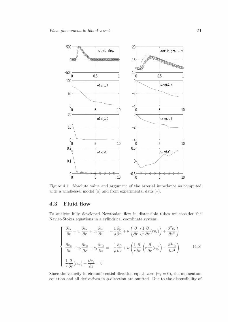
Wave phenomena in blood vessels 51
0 0.5 1−500
0
500
0 0.5 110
15
20
0 5 100
50
100
0 5 10−4
−2
0
0 5 100
10
20
0 5 10−4
−2
0
0 5 100
0.1
0.2
0 5 10−0.5
0
0.5
arg(qa)arg(pa)
aortic owabs(qa)
aortic pressure
abs(pa)abs(Z) arg(Z)
Figure 4.1: Absolute value and argument of the arterial impedance as computedwith a windkessel model (o) and from experimental data (–).
4.3 Fluid flow
To analyze fully developed Newtonian flow in distensible tubes we consider theNavier-Stokes equations in a cylindrical coordinate system:
∂vr∂t
+ vr∂vr∂r
+ vz∂vr∂z
= −1
ρ
∂p
∂r+ ν
(
∂
∂r
(
1
r
∂
∂r(rvr)
)
+∂2vr∂z2
)
∂vz∂t
+ vr∂vz∂r
+ vz∂vz∂z
= −1
ρ
∂p
∂z+ ν
(
1
r
∂
∂r
(
r∂
∂r(vz)
)
+∂2vz∂z2
)
1
r
∂
∂r(rvr) +
∂vz∂z
= 0
(4.5)
Since the velocity in circumferential direction equals zero (vφ = 0), the momentumequation and all derivatives in φ-direction are omitted. Due to the distensibility of
52 Cardiovascular Fluid Mechanics - lecture notes
the tube, pressure and flow waves will propagate with a finite wave speed c = ω/krand a typical wavelength λ = 2π/kr. First a properly scaled dimensionless form ofthe Navier-Stokes equations will be derived. To this end the radial coordinates aremade dimensionless using the mean radius of the tube, i.e. r′ = r/a0. The axialcoordinates, however, must be scaled with the real part of the wave number kr:z′ = zkr (see (4.3)). The axial velocity is made dimensionless with its characteristicvalue over a cross-section: v′z = vz/V . From the continuity equation it can be derivedthat the radial velocity then must be made dimensionless as: v′r = (vr/V )(1/kra).The characteristic time t′ = ωt can be written as t′ = (krc)t with c the wave speed.Together with a dimensionless pressure p′ = p/(ρV c) the dimensionless Navier-Stokes equations read:
∂v′r∂t′
+V
c
(
v′r∂v′r∂r′
+ v′z∂v′r∂z′
)
=
− 1
k2ra20
∂p′
∂r′+
1
α2
(
∂
∂r′
(
1
r′∂
∂r′(r′v′r)
)
+ a20k2r
∂2v′r∂z′2
)
∂v′z∂t′
+V
c
(
v′r∂v′z∂r′
+ v′z∂v′z∂z′
)
=
−∂p′
∂z′+
1
α2
(
1
r′∂
∂r′
(
r′∂
∂r′(v′z)
)
+ a20k2r
∂2v′z∂z′2
)
1
r′∂
∂r′(r′v′r) +
∂v′z∂z′
= 0
(4.6)
Besides the Womersley parameter α = a0√
ω/ν the dimensionless parameters thatplay a role in this equation are the speed ratio S = V/c and the circumference-to-wavelength ratio G = a0kr = 2πa0/λ. Under the assumptions that the wave velocityc is much larger then the fluid velocity V , the wavelength λ is much larger then thetube radius a0 ,i.e.:
S =V
c≪ 1, G2 = (kra0)
2 = (2πa0λ
)2 ≪ 1 (4.7)
it can readily be shown that the equations of motion reduce to:
∂p
∂r= 0
∂vz∂t
= −1
ρ
∂p
∂z+ ν
1
r
∂
∂r
(
r∂vz∂r
)
1
r
∂
∂r(rvr) +
∂vz∂z
= 0
(4.8)
If we search for harmonic solutions with angular frequency ω and wave number k:
p = pei(ωt−kz) (4.9)
Wave phenomena in blood vessels 53
and
vz = vz(r)ei(ωt−kz) (4.10)
substitution in equation (4.8) yields exactly the same differential equation for vz asin the case of a rigid tube given in equation (2.22). If we further assume that thewall motion is axially restrained, which is thought to be relevant in vivo (Pedley,1980), also the boundary condition for vz is not different from the one in rigid tubesbut now must be applied in a linearized way at r = a0. It will be clear that inthat case we obtain exactly the same Womersley solution given by equation (2.22).Substitution of:
∂p
∂z= −ikp (4.11)
yields:
vz(r) =k
ρω
[
1− J0(i3/2αr/a0)
J0(i3/2α)
]
p (4.12)
In Womersley (1957) a relation similar to (4.12) is derived, however without theassumption of axial constraint. In that case the second term in the brackets ismultiplied with an extra parameter that only slightly differs from unity. The wallshear stress is equal to the wall shear stress for rigid tubes and is defined by equation(2.35). The wave number k still has to be determined and depends on the propertiesof the arterial wall. In the next section the wall motion will be analyzed, againassuming axial restraint.
4.4 Wave propagation
4.4.1 Derivation of a quasi one-dimensional model
In order to obtain an expression for the wave number introduced in the previoussection, a quasi one-dimensional wave propagation model for pressure and flow waveswill be derived. To this end the Leibnitz formulae (or Reynolds transport theorem)will be used to integrate the equations of motion given in (4.8). This formulae wasderived in appendix A (equation A.32). A more suitable form for the application inthis chapter is:
d
dz
a(z)∫
0
s(r, z)dr =
a(z)∫
0
∂s(r, z)
∂zdr + s(a, z)
∂a
∂z|a (4.13)
See also figure 4.2.Application to the second term of the continuity equation in (4.8) integrated overthe radius:
2π
a(z)∫
0
1
r
∂
∂r(rvr)rdr +
a(z)∫
0
∂vz∂z
rdr
= 0 (4.14)
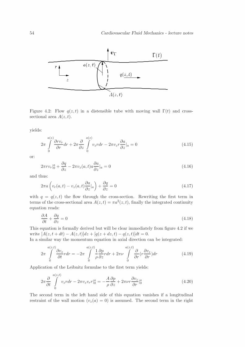
54 Cardiovascular Fluid Mechanics - lecture noteszr q(z; t)va(z; t) (t)A(z; t)Figure 4.2: Flow q(z, t) in a distensible tube with moving wall Γ(t) and cross-sectional area A(z, t).
yields:
2π
a(z)∫
0
∂rvr∂r
dr + 2π∂
∂z
a(z)∫
0
vzrdr − 2πvzr∂a
∂z|a = 0 (4.15)
or:
2πrvr|a0 +∂q
∂z− 2πvz(a, t)a
∂a
∂z|a = 0 (4.16)
and thus:
2πa
(
vr(a, t)− vz(a, t)∂a
∂z|a)
+∂q
∂z= 0 (4.17)
with q = q(z, t) the flow through the cross-section. Rewriting the first term interms of the cross-sectional area A(z, t) = πa2(z, t), finally the integrated continuityequation reads:
∂A
∂t+∂q
∂z= 0 (4.18)
This equation is formally derived but will be clear immediately from figure 4.2 if wewrite [A(z, t+ dt)−A(z, t)]dz + [q(z + dz, t)− q(z, t)]dt = 0.In a similar way the momentum equation in axial direction can be integrated:
2π
a(z,t)∫
0
∂vz∂t
rdr = −2π
a(z,t)∫
0
1
ρ
∂p
∂zrdr + 2πν
a(z,t)∫
0
∂
∂r(r∂vz∂r
)dr (4.19)
Application of the Leibnitz formulae to the first term yields:
2π∂
∂t
a(z,t)∫
0
vzrdr − 2πvzvrr|a0 = −Aρ
∂p
∂z+ 2πνr
∂vz∂r
|a0 (4.20)
The second term in the left hand side of this equation vanishes if a longitudinalrestraint of the wall motion (vz(a) = 0) is assumed. The second term in the right
Wave phenomena in blood vessels 55
hand side can be written in terms of the wall shear stress defined in equation (2.25).The integrated momentum equation then reads:
ρ∂q
∂t+A
∂p
∂z= −2Aτ
a(4.21)
Together with the expression for the wall shear stress given in (2.35) and linearisationof the A∂p
∂z term we finally obtain:
ρ∂q
∂t+A0
∂p
∂z= −f0q (4.22)
with f0 a friction function defined as:
f0(ω) = iωρF10(ω)
1− F10(ω)(4.23)
The linearized one-dimensional equations that describe the pressure and flow indistensible tubes under the assumption that V/c≪ 1, (2πa/λ)2 ≪ 1 and under theassumption that the wall motion is longitudinally constrained thus are given by:
C0∂p
∂t+∂q
∂z= 0
ρ∂q
∂t+A0
∂p
∂z= −f0q
(4.24)
with C0 the linearized compliance given by:
C0 = (∂A
∂p)p=p0 (4.25)
Alternatively using the mean velocity v instead of the flow q = Av:
D0∂p
∂t+∂v
∂z= 0
ρ∂v
∂t+∂p
∂z= −f0v
(4.26)
with D0 a linearized distensibility given by:
D0 =1
A0(∂A
∂p)p=p0 (4.27)
In the next section we will derive the wave number k for inviscid, viscosity domi-nated and general flow (i.e. large, small and intermediate values of the Womersleyparameter α).
56 Cardiovascular Fluid Mechanics - lecture notes
4.4.2 Wave speed and attenuation constant
The linearized one-dimensional mass and momentum equations for unsteady viscousflow through a distensible tube has been derived by integrating the continuity andmomentum equations over a cross-section of the tube assuming the wave-length tobe large compared to the diameter of the tube and the phase velocity of the waveto be large compared to the mean fluid velocity. Moreover it is assumed that themotion of the tube wall is restrained longitudinally. Due to the linearity assumed,the resulting equations (4.18) and (4.22) can be solved in the frequency domain bysubstituting harmonic solutions
p(ω, z, t) = p(ω, 0)ei(ωt−kz) (4.28)
q(ω, z, t) = q(ω, 0)ei(ωt−kz) (4.29)
A(ω, z, t) = A(ω, 0)ei(ωt−kz) (4.30)
where p(ω, 0), q(ω, 0) and A(ω, 0) are the complex amplitudes representing both theamplitude and the phase of the waves measured at location z = 0, ω is the angularfrequency and k(ω) is the wave number ; a complex number defined by:
k(ω) =ω
c− i
γ(ω)
λ(4.31)
Here c denotes the phase velocity of the waves and the wave length is given byλ = 2πc/ω. The exponential decrease of the amplitude of the waves is described bythe attenuation constant γ(ω) = −2πki/kr.
Viscoelastic wall behavior is described by an experimentally determined constitutiverelationship between the cross-sectional area A and the complex amplitude p:
A = C(ω)p (4.32)
where C(ω) is the dynamic compliance. For thin walled visco-elastic tubes thisrelationship can also be derived from equations (3.26) using a complex Young’smodulus E = Er + iEi.
Large Womersley number flow
For large Womersley parameters the flow will be inviscid and the friction functionf0 can be neglected. Substitution of (4.28-4.30) in (4.24) yields:
iωC(ω)p− ik(ω)q = 0
−ik(ω)A0p+ iωρq = 0(4.33)
with solution:
k0(ω) = ±√
ω2ρC(ω)
A0= ± ω
c0(4.34)
Wave phenomena in blood vessels 57
where the positive (negative) sign holds for waves traveling in the positive (negative)z-direction and c0 denotes the Moens-Korteweg wave speed given by:
c0(ω) =
√
A0
ρC(ω)=
√
1
ρD0(ω). (4.35)
Note that the subscript 0 is used in k0 and c0 in order to obey conventions inliterature despite the fact that k∞ and c∞ would be more meaningful since α→ ∞.For thin walled tubes the Moens-Korteweg wave speed can be derived from 3.26)and reads:
c0 =
√
1
ρ
hE
2a0(1− µ2)(4.36)
Note that the wave number k0 = ω/c0 is a real number expressing that the phasevelocity c equals the Moens-Korteweg wave speed and that the attenuation constantγ equals zero:
α→ ∞ : c(ω) = c0, γ(ω) = 0. (4.37)
As there is no friction and the compliance is assumed to be real (no visco-elasticity),no attenuation (γ(ω) = 0) of the wave will occur. The corresponding wave equationcan be derived form (4.24): after elimination of the flow and keeping in mind thatthe friction function is neglected we obtain the differential equation:
∂2p
∂t2− 1
ρD0
∂2p
∂z2= 0 (4.38)
This is a wave equation with wave speed c0 =√
1/ρD0 . So for large α and real valuesfor the distensibility D0 the pressure wave travels without damping in z-direction.
Equation (4.33) can also be solved with respect to the ratio q/p between the flowand the pressure:
Y0 =q
p= C(ω)
ω
k(ω)= ±A0
ρc0(4.39)
This ratio is referred to as the admittance Y0 and is equal to the reciprocal value ofthe impedance:
Y ≡ 1
Z≡ q
p(4.40)
As k(ω) represents two waves (one wave traveling in positive z-direction (k > 0)and one wave traveling in negative z-direction (k < 0)) there are two flow andpressure waves: forward traveling waves qf = +Y pf and backward traveling wavesqb = −Y pb. The total pressure and flow is the sum of these waves p(z, t) = pf (z, t)+pb(z, t) resp. q(z, t) = qf (z, t) + qb(z, t).
58 Cardiovascular Fluid Mechanics - lecture notes
Small Womersley number flow
For small Womersley parameters the flow will be dominated by viscous forces andthe friction function f0 can be approximated by its Poiseuille value f0 = 8η/a20whereas the instationary inertia forces in the momentum equation can be neglected.Substitution of (4.28-4.30) in (4.24) yields:
iωC(ω)p− ik(ω)q = 0
−ik(ω)A0p+8η
a20q = 0
(4.41)
and has a non-trivial solution if:
k(ω) = ±√
−8iηωC(ω)
A0a20
= ± ω
c0
√
−8i
α2= ±2(1− i)
αk0 (4.42)
where the positive (negative) sign now holds for waves traveling in the positive(negative) z-direction and c0 denotes the Moens-Korteweg wave speed.
Now the wave number is a complex number and the phase velocity c and attenuationconstant γ are given by:
α→ 0 : c(ω) = 12αc0, γ(ω) = 2π. (4.43)
As the real and imaginary part of the wave number are equal, the wave is dampedcritically. This can also be seen from (4.24): after elimination of the flow andkeeping in mind that the instationary inertia forces can be neglected we obtain thedifferential equation:
∂p
∂t=A0a
20
8ηC0
∂2p
∂z2=
a208ηD0
∂2p
∂z2(4.44)
This is a diffusion equation with diffusion coefficient D = a20/8ηD0. So for small αthe wave equation reduces to a diffusion equation showing critical damping of thepressure in z-direction. This phenomena is responsible for the large pressure dropthat is found in the micro-circulation where the Womersley parameter is low as aresult of the small diameters of the vessels.
The admittance Y now is a complex number given by:
Y = ±A0
ρc0
i+ 1
4α =
i+ 1
4αY0 (4.45)
Arbitrary Womersley number flow
Substitution of equations (4.28-4.30), (4.32) and (4.23) in equations (4.18) and (4.22)yields:
iωC(ω)p− ik(ω)q = 0
−ik(ω)A0p+ (iωρ+ f0)q = 0(4.46)
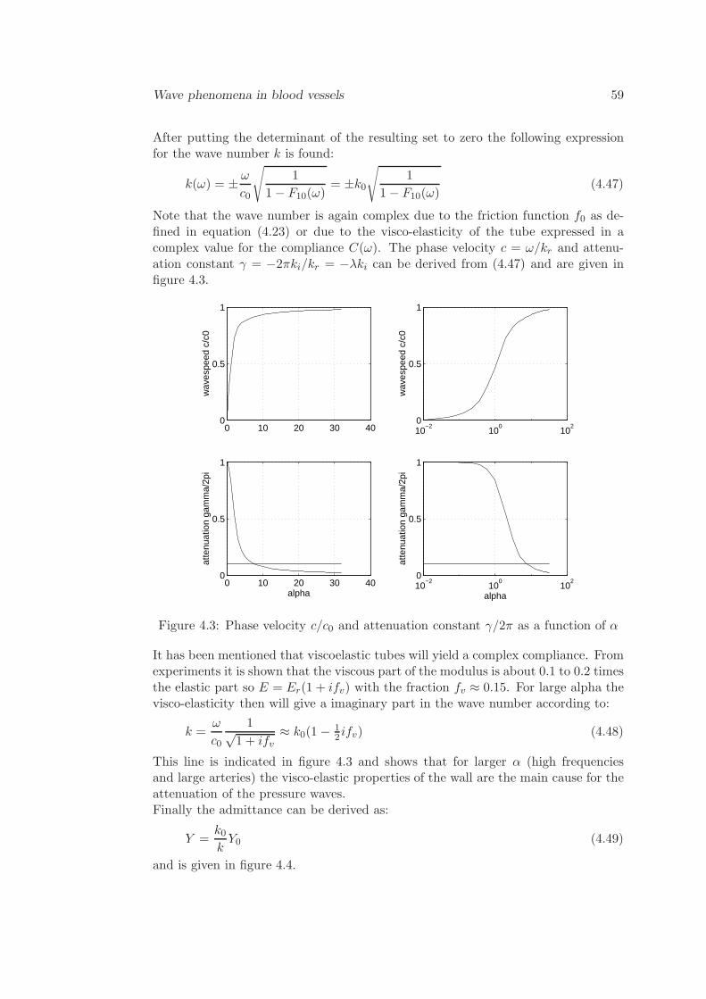
Wave phenomena in blood vessels 59
After putting the determinant of the resulting set to zero the following expressionfor the wave number k is found:
k(ω) = ± ω
c0
√
1
1− F10(ω)= ±k0
√
1
1− F10(ω)(4.47)
Note that the wave number is again complex due to the friction function f0 as de-fined in equation (4.23) or due to the visco-elasticity of the tube expressed in acomplex value for the compliance C(ω). The phase velocity c = ω/kr and attenu-ation constant γ = −2πki/kr = −λki can be derived from (4.47) and are given infigure 4.3.
0 10 20 30 400
0.5
1
wav
espe
ed c
/c0
0 10 20 30 400
0.5
1
alpha
atte
nuat
ion
gam
ma/
2pi
10−2
100
102
0
0.5
1
wav
espe
ed c
/c0
10−2
100
102
0
0.5
1
alpha
atte
nuat
ion
gam
ma/
2pi
Figure 4.3: Phase velocity c/c0 and attenuation constant γ/2π as a function of α
It has been mentioned that viscoelastic tubes will yield a complex compliance. Fromexperiments it is shown that the viscous part of the modulus is about 0.1 to 0.2 timesthe elastic part so E = Er(1 + ifv) with the fraction fv ≈ 0.15. For large alpha thevisco-elasticity then will give a imaginary part in the wave number according to:
k =ω
c0
1√1 + ifv
≈ k0(1− 12 ifv) (4.48)
This line is indicated in figure 4.3 and shows that for larger α (high frequenciesand large arteries) the visco-elastic properties of the wall are the main cause for theattenuation of the pressure waves.Finally the admittance can be derived as:
Y =k0kY0 (4.49)
and is given in figure 4.4.
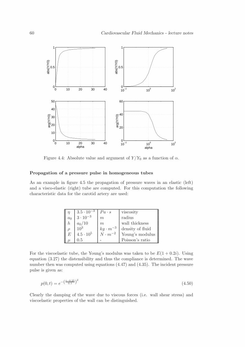
60 Cardiovascular Fluid Mechanics - lecture notes
0 10 20 30 400
0.5
1ab
s(Y
/Y0)
0 10 20 30 400
10
20
30
40
50
alpha
arg(
Y/Y
0)
10−2
100
102
0
0.5
1
abs(
Y/Y
0)
10−2
100
102
0
20
40
60
alpha
arg(
Y/Y
0)
Figure 4.4: Absolute value and argument of Y/Y0 as a function of α.
Propagation of a pressure pulse in homogeneous tubes
As an example in figure 4.5 the propagation of pressure waves in an elastic (left)and a visco-elastic (right) tube are computed. For this computation the followingcharacteristic data for the carotid artery are used:
η 3.5 · 10−3 Pa · s viscositya0 3 · 10−3 m radiush a0/10 m wall thicknessρ 103 kg ·m−3 density of fluidE 4.5 · 105 N ·m−2 Young’s modulusµ 0.5 - Poisson’s ratio
For the viscoelastic tube, the Young’s modulus was taken to be E(1 + 0.2i). Usingequation (3.27) the distensibility and thus the compliance is determined. The wavenumber then was computed using equations (4.47) and (4.35). The incident pressurepulse is given as:
p(0, t) = e−(t−0.25
0.1 )2
(4.50)
Clearly the damping of the wave due to viscous forces (i.e. wall shear stress) andviscoelastic properties of the wall can be distinguished.
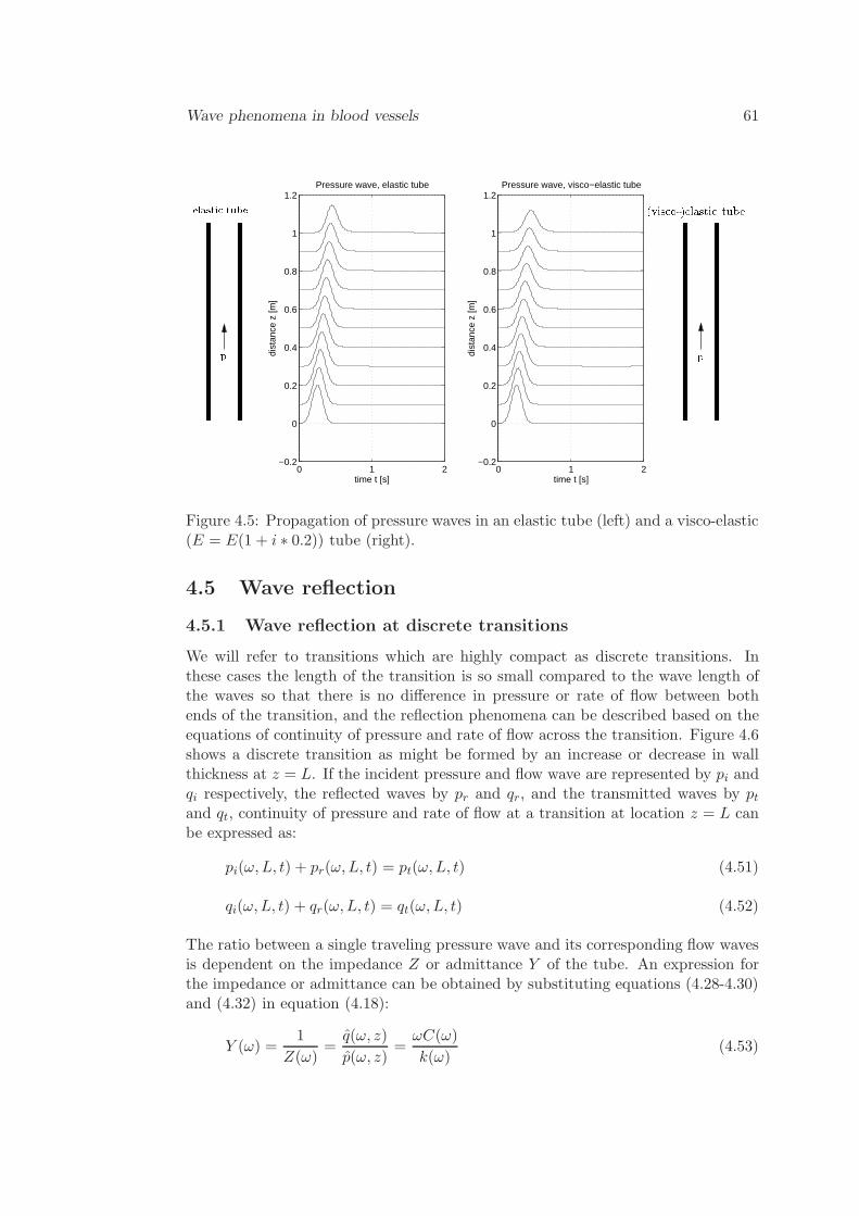
Wave phenomena in blood vessels 61
0 1 2−0.2
0
0.2
0.4
0.6
0.8
1
1.2
time t [s]
dist
ance
z [m
]
Pressure wave, elastic tube
0 1 2−0.2
0
0.2
0.4
0.6
0.8
1
1.2
time t [s]di
stan
ce z
[m]
Pressure wave, visco−elastic tube (visco-)elastic tubep pelastic tubeFigure 4.5: Propagation of pressure waves in an elastic tube (left) and a visco-elastic(E = E(1 + i ∗ 0.2)) tube (right).
4.5 Wave reflection
4.5.1 Wave reflection at discrete transitions
We will refer to transitions which are highly compact as discrete transitions. Inthese cases the length of the transition is so small compared to the wave length ofthe waves so that there is no difference in pressure or rate of flow between bothends of the transition, and the reflection phenomena can be described based on theequations of continuity of pressure and rate of flow across the transition. Figure 4.6shows a discrete transition as might be formed by an increase or decrease in wallthickness at z = L. If the incident pressure and flow wave are represented by pi andqi respectively, the reflected waves by pr and qr, and the transmitted waves by ptand qt, continuity of pressure and rate of flow at a transition at location z = L canbe expressed as:
pi(ω,L, t) + pr(ω,L, t) = pt(ω,L, t) (4.51)
qi(ω,L, t) + qr(ω,L, t) = qt(ω,L, t) (4.52)
The ratio between a single traveling pressure wave and its corresponding flow wavesis dependent on the impedance Z or admittance Y of the tube. An expression forthe impedance or admittance can be obtained by substituting equations (4.28-4.30)and (4.32) in equation (4.18):
Y (ω) =1
Z(ω)=q(ω, z)
p(ω, z)=ωC(ω)
k(ω)(4.53)
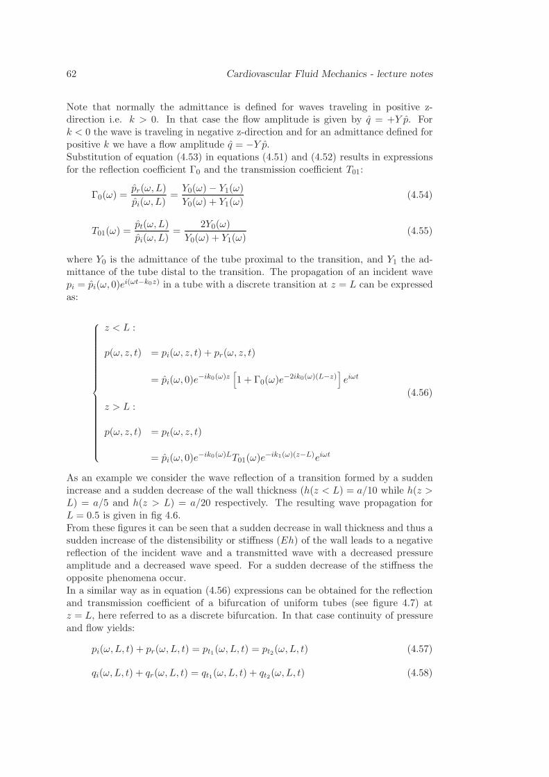
62 Cardiovascular Fluid Mechanics - lecture notes
Note that normally the admittance is defined for waves traveling in positive z-direction i.e. k > 0. In that case the flow amplitude is given by q = +Y p. Fork < 0 the wave is traveling in negative z-direction and for an admittance defined forpositive k we have a flow amplitude q = −Y p.Substitution of equation (4.53) in equations (4.51) and (4.52) results in expressionsfor the reflection coefficient Γ0 and the transmission coefficient T01:
Γ0(ω) =pr(ω,L)
pi(ω,L)=Y0(ω)− Y1(ω)
Y0(ω) + Y1(ω)(4.54)
T01(ω) =pt(ω,L)
pi(ω,L)=
2Y0(ω)
Y0(ω) + Y1(ω)(4.55)
where Y0 is the admittance of the tube proximal to the transition, and Y1 the ad-mittance of the tube distal to the transition. The propagation of an incident wavepi = pi(ω, 0)e
i(ωt−k0z) in a tube with a discrete transition at z = L can be expressedas:
z < L :
p(ω, z, t) = pi(ω, z, t) + pr(ω, z, t)
= pi(ω, 0)e−ik0(ω)z
[
1 + Γ0(ω)e−2ik0(ω)(L−z)
]
eiωt
z > L :
p(ω, z, t) = pt(ω, z, t)
= pi(ω, 0)e−ik0(ω)LT01(ω)e
−ik1(ω)(z−L)eiωt
(4.56)
As an example we consider the wave reflection of a transition formed by a suddenincrease and a sudden decrease of the wall thickness (h(z < L) = a/10 while h(z >L) = a/5 and h(z > L) = a/20 respectively. The resulting wave propagation forL = 0.5 is given in fig 4.6.
From these figures it can be seen that a sudden decrease in wall thickness and thus asudden increase of the distensibility or stiffness (Eh) of the wall leads to a negativereflection of the incident wave and a transmitted wave with a decreased pressureamplitude and a decreased wave speed. For a sudden decrease of the stiffness theopposite phenomena occur.In a similar way as in equation (4.56) expressions can be obtained for the reflectionand transmission coefficient of a bifurcation of uniform tubes (see figure 4.7) atz = L, here referred to as a discrete bifurcation. In that case continuity of pressureand flow yields:
pi(ω,L, t) + pr(ω,L, t) = pt1(ω,L, t) = pt2(ω,L, t) (4.57)
qi(ω,L, t) + qr(ω,L, t) = qt1(ω,L, t) + qt2(ω,L, t) (4.58)
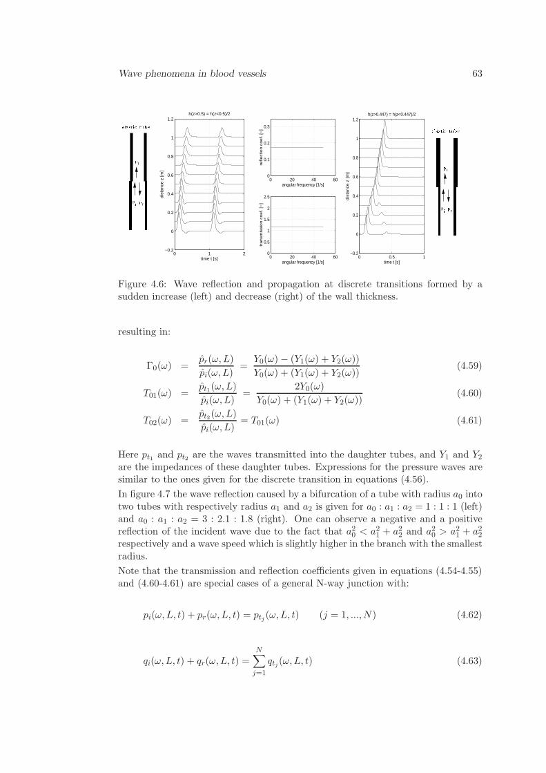
Wave phenomena in blood vessels 63
0 1 2−0.2
0
0.2
0.4
0.6
0.8
1
1.2
time t [s]
dist
ance
z [m
]
h(z>0.5) = h(z<0.5)/2
0 20 40 600
0.1
0.2
0.3
angular frequency [1/s]
refle
ctio
n c
oe
f. [
−]
0 20 40 600
0.5
1
1.5
2
2.5
angular frequency [1/s]tr
an
smis
sio
n c
oe
f. [
−]
0 0.5 1−0.2
0
0.2
0.4
0.6
0.8
1
1.2
time t [s]
dis
tan
ce z
[m
]
h(z>0.447) = h(z<0.447)/2
pr
t
pr
t
pi pelastic tube pi pelastic tubeFigure 4.6: Wave reflection and propagation at discrete transitions formed by asudden increase (left) and decrease (right) of the wall thickness.
resulting in:
Γ0(ω) =pr(ω,L)
pi(ω,L)=
Y0(ω)− (Y1(ω) + Y2(ω))
Y0(ω) + (Y1(ω) + Y2(ω))(4.59)
T01(ω) =pt1(ω,L)
pi(ω,L)=
2Y0(ω)
Y0(ω) + (Y1(ω) + Y2(ω))(4.60)
T02(ω) =pt2(ω,L)
pi(ω,L)= T01(ω) (4.61)
Here pt1 and pt2 are the waves transmitted into the daughter tubes, and Y1 and Y2are the impedances of these daughter tubes. Expressions for the pressure waves aresimilar to the ones given for the discrete transition in equations (4.56).
In figure 4.7 the wave reflection caused by a bifurcation of a tube with radius a0 intotwo tubes with respectively radius a1 and a2 is given for a0 : a1 : a2 = 1 : 1 : 1 (left)and a0 : a1 : a2 = 3 : 2.1 : 1.8 (right). One can observe a negative and a positivereflection of the incident wave due to the fact that a20 < a21 + a22 and a20 > a21 + a22respectively and a wave speed which is slightly higher in the branch with the smallestradius.
Note that the transmission and reflection coefficients given in equations (4.54-4.55)and (4.60-4.61) are special cases of a general N-way junction with:
pi(ω,L, t) + pr(ω,L, t) = ptj (ω,L, t) (j = 1, ..., N) (4.62)
qi(ω,L, t) + qr(ω,L, t) =N∑
j=1
qtj (ω,L, t) (4.63)
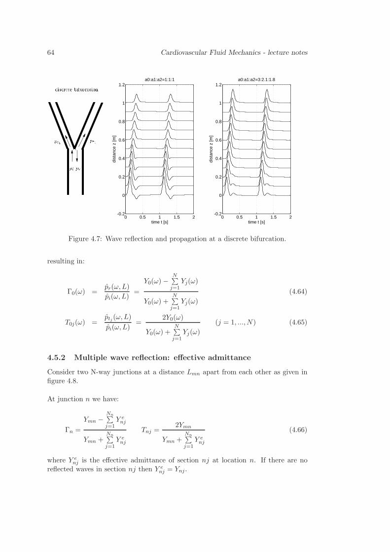
64 Cardiovascular Fluid Mechanics - lecture notes
0 0.5 1 1.5 2-0.2
0
0.2
0.4
0.6
0.8
1
1.2
time t [s]
dist
ance
z [m
]
a0:a1:a2=1:1:1
0 0.5 1 1.5 2-0.2
0
0.2
0.4
0.6
0.8
1
1.2
time t [s]
dist
ance
z [m
]
a0:a1:a2=3:2.1:1.8pt2 pi prdiscrete bifurcationpt1
Figure 4.7: Wave reflection and propagation at a discrete bifurcation.
resulting in:
Γ0(ω) =pr(ω,L)
pi(ω,L)=
Y0(ω)−N∑
j=1Yj(ω)
Y0(ω) +N∑
j=1Yj(ω)
(4.64)
T0j(ω) =ptj (ω,L)
pi(ω,L)=
2Y0(ω)
Y0(ω) +N∑
j=1Yj(ω)
(j = 1, ..., N) (4.65)
4.5.2 Multiple wave reflection: effective admittance
Consider two N-way junctions at a distance Lmn apart from each other as given infigure 4.8.
At junction n we have:
Γn =
Ymn −Nn∑
j=1Y enj
Ymn +Nn∑
j=1Y enj
Tnj =2Ymn
Ymn +Nn∑
j=1Y enj
(4.66)
where Y enj is the effective admittance of section nj at location n. If there are no
reflected waves in section nj then Y enj = Ynj .
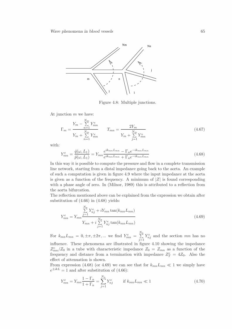
Wave phenomena in blood vessels 65
m n
1
Nm
1
j
Nn
Figure 4.8: Multiple junctions.
At junction m we have:
Γm =
Ym −Nm∑
n=1Y emn
Ym +Nm∑
n=1Y emn
Tmn =2Ym
Ym +Nm∑
j=1Y emn
(4.67)
with:
Y emn =
q(ω,L1)
p(ω,L1)= Ymn
eikmnLmn − Γne−ikmnLmn
eikmnLmn + Γne−ikmnLmn(4.68)
In this way it is possible to compute the pressure and flow in a complete transmissionline network, starting from a distal impedance going back to the aorta. An exampleof such a computation is given in figure 4.9 where the input impedance at the aortais given as a function of the frequency. A minimum of |Z| is found correspondingwith a phase angle of zero. In (Milnor, 1989) this is attributed to a reflection fromthe aorta bifurcation.The reflection mentioned above can be explained from the expression we obtain aftersubstitution of (4.66) in (4.68) yields:
Y emn = Ymn
Nn∑
j=1Y enj + iYmn tan(kmnLmn)
Ymn + iNn∑
j=1Y enj tan(kmnLmn)
(4.69)
For kmnLmn = 0,±π,±2π, ... we find Y emn =
Nn∑
j=1Y enj and the section mn has no
influence. These phenomena are illustrated in figure 4.10 showing the impedanceZemn/Z0 in a tube with characteristic impedance Z0 = Zmn as a function of the
frequency and distance from a termination with impedance ZeT = 4Z0. Also the
effect of attenuation is shown.From expression (4.68) (or 4.69) we can see that for kmnLmn ≪ 1 we simply havee±ikL = 1 and after substitution of (4.66):
Y emn = Ymn
1− Γn
1 + Γn=
Nn∑
j=1
Y enj if kmnLmn ≪ 1 (4.70)
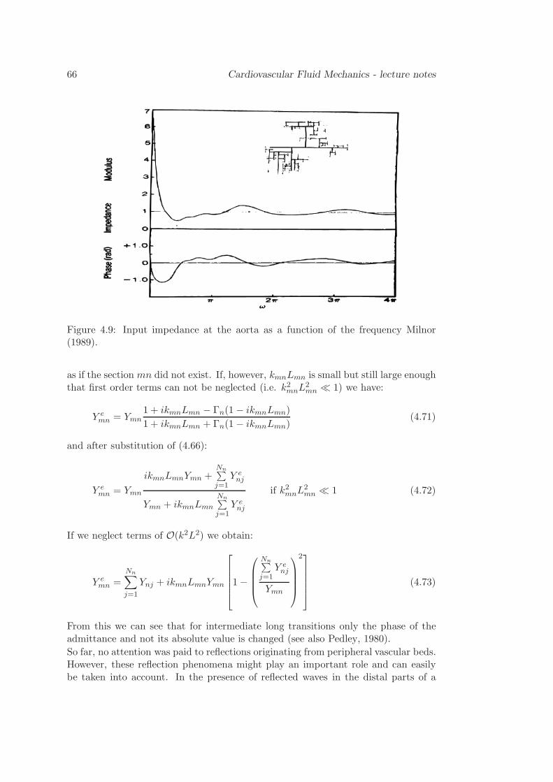
66 Cardiovascular Fluid Mechanics - lecture notes
Figure 4.9: Input impedance at the aorta as a function of the frequency Milnor(1989).
as if the section mn did not exist. If, however, kmnLmn is small but still large enoughthat first order terms can not be neglected (i.e. k2mnL
2mn ≪ 1) we have:
Y emn = Ymn
1 + ikmnLmn − Γn(1− ikmnLmn)
1 + ikmnLmn + Γn(1− ikmnLmn)(4.71)
and after substitution of (4.66):
Y emn = Ymn
ikmnLmnYmn +Nn∑
j=1Y enj
Ymn + ikmnLmn
Nn∑
j=1Y enj
if k2mnL2mn ≪ 1 (4.72)
If we neglect terms of O(k2L2) we obtain:
Y emn =
Nn∑
j=1
Ynj + ikmnLmnYmn
1−
Nn∑
j=1Y enj
Ymn
2
(4.73)
From this we can see that for intermediate long transitions only the phase of theadmittance and not its absolute value is changed (see also Pedley, 1980).
So far, no attention was paid to reflections originating from peripheral vascular beds.However, these reflection phenomena might play an important role and can easilybe taken into account. In the presence of reflected waves in the distal parts of a
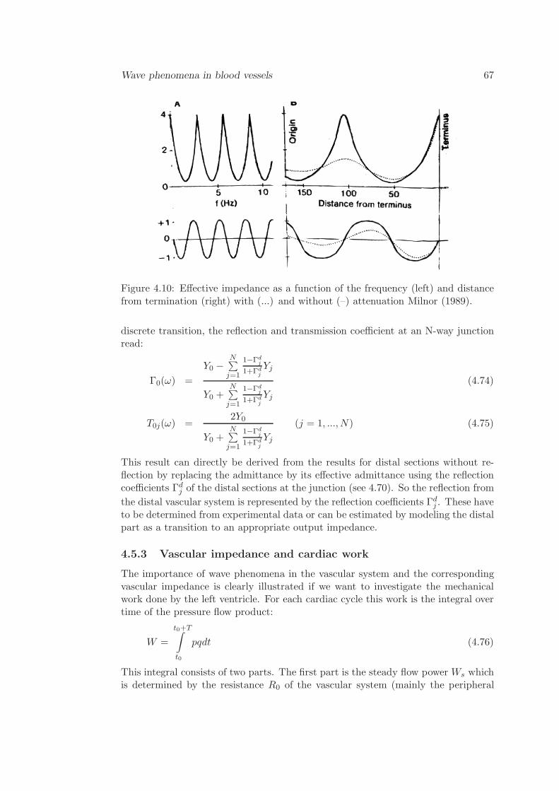
Wave phenomena in blood vessels 67
Figure 4.10: Effective impedance as a function of the frequency (left) and distancefrom termination (right) with (...) and without (–) attenuation Milnor (1989).
discrete transition, the reflection and transmission coefficient at an N-way junctionread:
Γ0(ω) =
Y0 −N∑
j=1
1−Γdj
1+Γdj
Yj
Y0 +N∑
j=1
1−Γdj
1+Γdj
Yj
(4.74)
T0j(ω) =2Y0
Y0 +N∑
j=1
1−Γdj
1+Γdj
Yj
(j = 1, ..., N) (4.75)
This result can directly be derived from the results for distal sections without re-flection by replacing the admittance by its effective admittance using the reflectioncoefficients Γd
j of the distal sections at the junction (see 4.70). So the reflection from
the distal vascular system is represented by the reflection coefficients Γdj . These have
to be determined from experimental data or can be estimated by modeling the distalpart as a transition to an appropriate output impedance.
4.5.3 Vascular impedance and cardiac work
The importance of wave phenomena in the vascular system and the correspondingvascular impedance is clearly illustrated if we want to investigate the mechanicalwork done by the left ventricle. For each cardiac cycle this work is the integral overtime of the pressure flow product:
W =
t0+T∫
t0
pqdt (4.76)
This integral consists of two parts. The first part is the steady flow power Ws whichis determined by the resistance R0 of the vascular system (mainly the peripheral
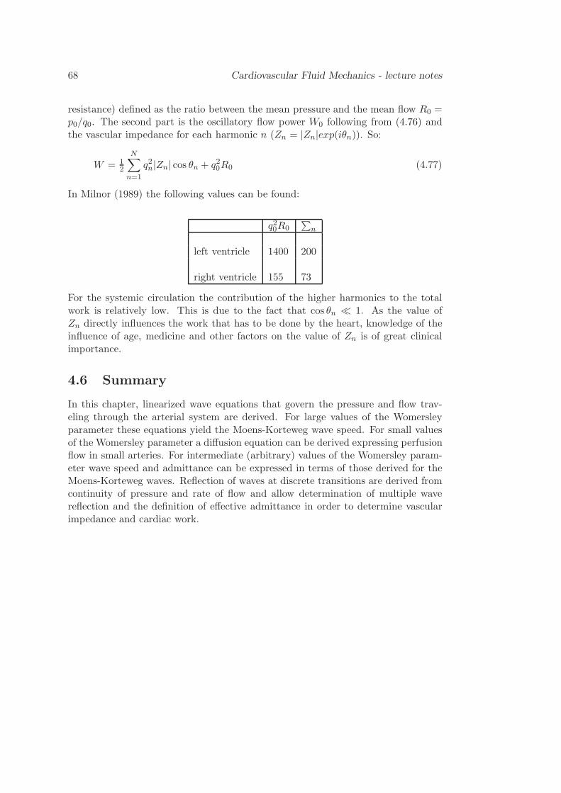
68 Cardiovascular Fluid Mechanics - lecture notes
resistance) defined as the ratio between the mean pressure and the mean flow R0 =p0/q0. The second part is the oscillatory flow power W0 following from (4.76) andthe vascular impedance for each harmonic n (Zn = |Zn|exp(iθn)). So:
W = 12
N∑
n=1
q2n|Zn| cos θn + q20R0 (4.77)
In Milnor (1989) the following values can be found:
q20R0∑
n
left ventricle 1400 200
right ventricle 155 73
For the systemic circulation the contribution of the higher harmonics to the totalwork is relatively low. This is due to the fact that cos θn ≪ 1. As the value ofZn directly influences the work that has to be done by the heart, knowledge of theinfluence of age, medicine and other factors on the value of Zn is of great clinicalimportance.
4.6 Summary
In this chapter, linearized wave equations that govern the pressure and flow trav-eling through the arterial system are derived. For large values of the Womersleyparameter these equations yield the Moens-Korteweg wave speed. For small valuesof the Womersley parameter a diffusion equation can be derived expressing perfusionflow in small arteries. For intermediate (arbitrary) values of the Womersley param-eter wave speed and admittance can be expressed in terms of those derived for theMoens-Korteweg waves. Reflection of waves at discrete transitions are derived fromcontinuity of pressure and rate of flow and allow determination of multiple wavereflection and the definition of effective admittance in order to determine vascularimpedance and cardiac work.
Chapter 5
Non-Newtonian flow in blood
vessels
5.1 Introduction
After a brief introduction to methods to measure fluid properties, in this chaptersequentially constitutive equations for Newtonian flow, generalized Newtonian flow,viscoelastic flow and the flow of suspensions will be dealt with. It will be shownthat the viscosity of blood is shear and history dependent as a result of the presenceof deformation and aggregation of the red blood cells that are suspended in plasma.The consequence of this non-Newtonian behavior on the velocity profiles in steadyand pulsatile flow will be illustrated.
69
70 Cardiovascular Fluid Mechanics - lecture notes
5.2 Mechanical properties of blood
Blood is a complex fluid consisting of blood cells suspended in plasma. The rheolog-ical behavior strongly depends in the properties of the suspended particles. In thissection some of the main aspects of blood rheology are given starting from a shortdescription of the morphology.
5.2.1 Morphology
Plasma is the continuous liquid medium in which the blood cells are suspended.It is an aqueous saline solution with proteins. The outline of the composition ofthe plasma is given in table 5.1. The density of plasma is 1.03 · 103 kg/m3. Ifdenaturisation of the proteins is avoided, plasma behaves like a Newtonian fluidwith a dynamic viscosity of η = 1.2 · 10−3Pa · s.The inorganic constituents of the plasma are a governing factor in various transportprocesses and generate an osmotic pressure of about 8∗105 Pa (equivalent to a 0.9%sodium chlorine solution by weight). The proteins have various functions and canbe divided into three groups:
fibrinogen : a large, asymmetric molecule which is intimately concerned with thecoagulation of blood. Although the concentration of fibrinogen is low, due toits asymmetry, it attributes significantly to the elevated viscosity of plasma.
albumin : a small molecule which is important for the osmotic pressure of theproteins.
globulins : a relatively symmetric molecule which is involved in transport of lipidsand antibody reactions.
Apart from the buffering function of all the proteins, both fibrinogen and the glob-ulins are involved in the aggregation of the erythrocytes.An outline of the composition of suspended blood cells is given in table 5.2.
The red blood cells, or erythrocytes, occupy 45 % of the blood volume and dominatethe rheological behavior of blood.
erythrocytes : form the dominant particulate matter of blood. The volume con-centration of the erythrocytes, called haematocrite, is about 45 %. The densityof the erythrocytes is 1.08 ∗103 kg/m3. The erythrocyte is a biconcave dis-coid and the main dimensions are given in figure 5.2.1. The membrane of theerythrocytes has a thickness of 80 nm and consists of a phospholipid bilayer.This bilayer is covered with albumin at the outside and with another layer ofprotein, spectrin, at the inside. The spectrin layer is a skeletal protein andsupports the lipid bilayer. The liquid interior of the erythrocyte is a saturatedsolution of hemoglobin (32 % by weight), behaving like a Newtonian fluid witha dynamic viscosity of η = 6·10−3Pa·s. The hemoglobin (MW = 68.000) is aprotein complex, consisting of an Fe2+ complex, the haem group, surroundedby amino acid molecules. The haem group is essential for transport processes
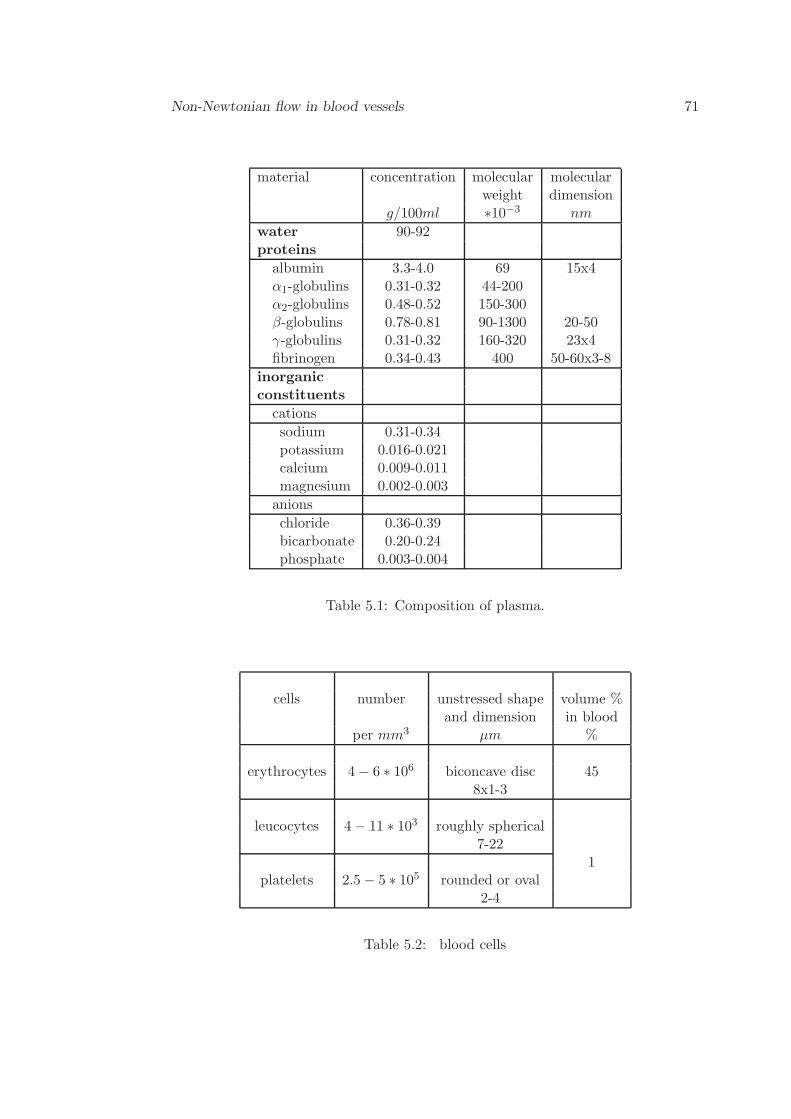
Non-Newtonian flow in blood vessels 71
material concentration molecular molecularweight dimension
g/100ml ∗10−3 nm
water 90-92proteins
albumin 3.3-4.0 69 15x4α1-globulins 0.31-0.32 44-200α2-globulins 0.48-0.52 150-300β-globulins 0.78-0.81 90-1300 20-50γ-globulins 0.31-0.32 160-320 23x4fibrinogen 0.34-0.43 400 50-60x3-8
inorganic
constituents
cations
sodium 0.31-0.34potassium 0.016-0.021calcium 0.009-0.011magnesium 0.002-0.003
anions
chloride 0.36-0.39bicarbonate 0.20-0.24phosphate 0.003-0.004
Table 5.1: Composition of plasma.
cells number unstressed shape volume %and dimension in blood
per mm3 µm %
erythrocytes 4− 6 ∗ 106 biconcave disc 458x1-3
leucocytes 4− 11 ∗ 103 roughly spherical7-22
1platelets 2.5− 5 ∗ 105 rounded or oval
2-4
Table 5.2: blood cells
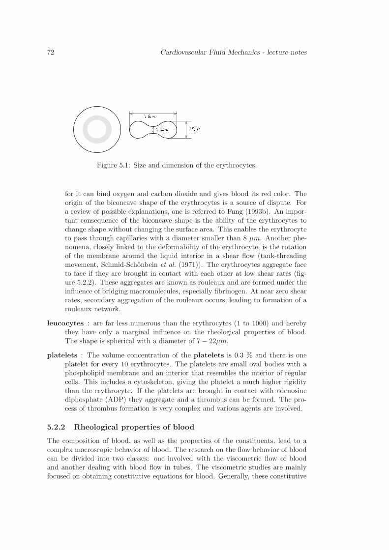
72 Cardiovascular Fluid Mechanics - lecture notes
2:8m1:2m7:8mFigure 5.1: Size and dimension of the erythrocytes.
for it can bind oxygen and carbon dioxide and gives blood its red color. Theorigin of the biconcave shape of the erythrocytes is a source of dispute. Fora review of possible explanations, one is referred to Fung (1993b). An impor-tant consequence of the biconcave shape is the ability of the erythrocytes tochange shape without changing the surface area. This enables the erythrocyteto pass through capillaries with a diameter smaller than 8 µm. Another phe-nomena, closely linked to the deformability of the erythrocyte, is the rotationof the membrane around the liquid interior in a shear flow (tank-threadingmovement, Schmid-Schonbein et al. (1971)). The erythrocytes aggregate faceto face if they are brought in contact with each other at low shear rates (fig-ure 5.2.2). These aggregates are known as rouleaux and are formed under theinfluence of bridging macromolecules, especially fibrinogen. At near zero shearrates, secondary aggregation of the rouleaux occurs, leading to formation of arouleaux network.
leucocytes : are far less numerous than the erythrocytes (1 to 1000) and herebythey have only a marginal influence on the rheological properties of blood.The shape is spherical with a diameter of 7− 22µm.
platelets : The volume concentration of the platelets is 0.3 % and there is oneplatelet for every 10 erythrocytes. The platelets are small oval bodies with aphospholipid membrane and an interior that resembles the interior of regularcells. This includes a cytoskeleton, giving the platelet a much higher rigiditythan the erythrocyte. If the platelets are brought in contact with adenosinediphosphate (ADP) they aggregate and a thrombus can be formed. The pro-cess of thrombus formation is very complex and various agents are involved.
5.2.2 Rheological properties of blood
The composition of blood, as well as the properties of the constituents, lead to acomplex macroscopic behavior of blood. The research on the flow behavior of bloodcan be divided into two classes: one involved with the viscometric flow of bloodand another dealing with blood flow in tubes. The viscometric studies are mainlyfocused on obtaining constitutive equations for blood. Generally, these constitutive
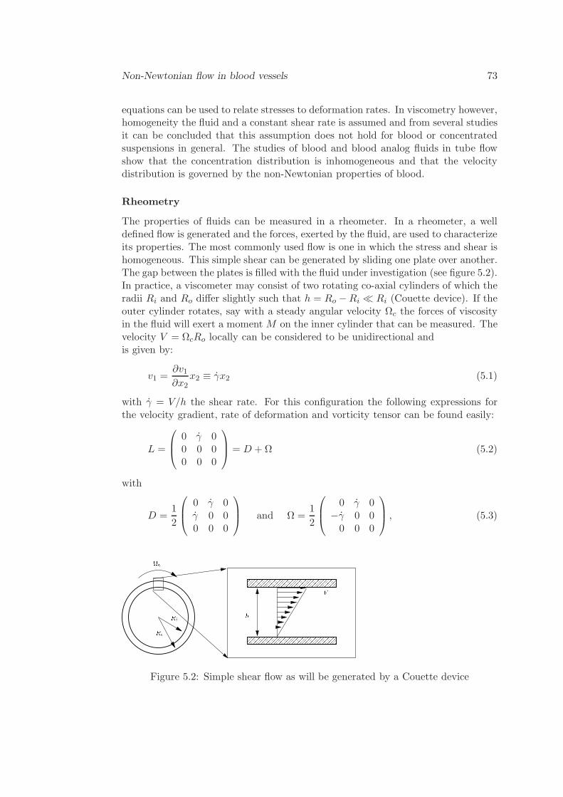
Non-Newtonian flow in blood vessels 73
equations can be used to relate stresses to deformation rates. In viscometry however,homogeneity the fluid and a constant shear rate is assumed and from several studiesit can be concluded that this assumption does not hold for blood or concentratedsuspensions in general. The studies of blood and blood analog fluids in tube flowshow that the concentration distribution is inhomogeneous and that the velocitydistribution is governed by the non-Newtonian properties of blood.
Rheometry
The properties of fluids can be measured in a rheometer. In a rheometer, a welldefined flow is generated and the forces, exerted by the fluid, are used to characterizeits properties. The most commonly used flow is one in which the stress and shear ishomogeneous. This simple shear can be generated by sliding one plate over another.The gap between the plates is filled with the fluid under investigation (see figure 5.2).In practice, a viscometer may consist of two rotating co-axial cylinders of which theradii Ri and Ro differ slightly such that h = Ro −Ri ≪ Ri (Couette device). If theouter cylinder rotates, say with a steady angular velocity Ωc the forces of viscosityin the fluid will exert a moment M on the inner cylinder that can be measured. Thevelocity V = ΩcRo locally can be considered to be unidirectional andis given by:
v1 =∂v1∂x2
x2 ≡ γx2 (5.1)
with γ = V/h the shear rate. For this configuration the following expressions forthe velocity gradient, rate of deformation and vorticity tensor can be found easily:
L =
0 γ 00 0 00 0 0
= D +Ω (5.2)
with
D =1
2
0 γ 0γ 0 00 0 0
and Ω =
1
2
0 γ 0−γ 0 00 0 0
, (5.3)
c RiRo h VFigure 5.2: Simple shear flow as will be generated by a Couette device
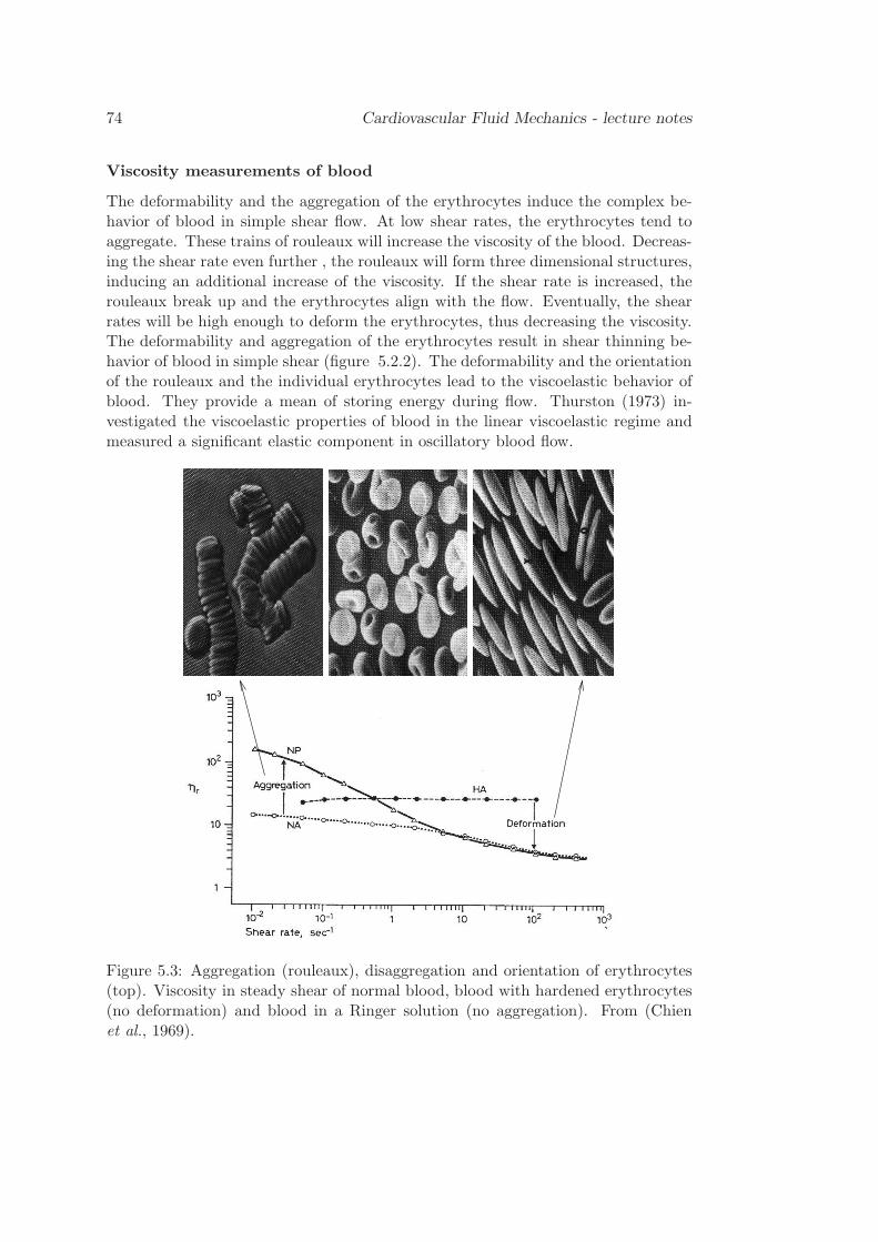
74 Cardiovascular Fluid Mechanics - lecture notes
Viscosity measurements of blood
The deformability and the aggregation of the erythrocytes induce the complex be-havior of blood in simple shear flow. At low shear rates, the erythrocytes tend toaggregate. These trains of rouleaux will increase the viscosity of the blood. Decreas-ing the shear rate even further , the rouleaux will form three dimensional structures,inducing an additional increase of the viscosity. If the shear rate is increased, therouleaux break up and the erythrocytes align with the flow. Eventually, the shearrates will be high enough to deform the erythrocytes, thus decreasing the viscosity.The deformability and aggregation of the erythrocytes result in shear thinning be-havior of blood in simple shear (figure 5.2.2). The deformability and the orientationof the rouleaux and the individual erythrocytes lead to the viscoelastic behavior ofblood. They provide a mean of storing energy during flow. Thurston (1973) in-vestigated the viscoelastic properties of blood in the linear viscoelastic regime andmeasured a significant elastic component in oscillatory blood flow.
Figure 5.3: Aggregation (rouleaux), disaggregation and orientation of erythrocytes(top). Viscosity in steady shear of normal blood, blood with hardened erythrocytes(no deformation) and blood in a Ringer solution (no aggregation). From (Chienet al., 1969).
Non-Newtonian flow in blood vessels 75
5.3 Newtonian models
5.3.1 Constitutive equations
As indicated in appendix A, a constitutive equation for fluids may have the form
σ = σ(B) = σ(2D). (5.4)
A general way to construct an arbitrary function σ(2D) is to expand the functionin a power series. This yields:
σ = f0D0 + f1D
1 + f2D2 + f3D
3 + ... (5.5)
The Cayley Hamilton theorem (Chadwick, 1976) states that for (any symmetric)tensor D it can be shown that:
D3 − IDD2 + IIDD − IIIDI = 0 (5.6)
Here ID, IID and IIID are the invariants of D defined as:
ID = trD
= D11 +D22 +D33
(5.7)
IID = 12(I
2D − trD2)
=
∣
∣
∣
∣
∣
D11 D12
D21 D22
∣
∣
∣
∣
∣
+
∣
∣
∣
∣
∣
D22 D23
D32 D23
∣
∣
∣
∣
∣
+
∣
∣
∣
∣
∣
D33 D31
D13 D11
∣
∣
∣
∣
∣
(5.8)
IIID = detD
=
∣
∣
∣
∣
∣
∣
∣
D11 D12 D13
D21 D22 D33
D31 D32 D33
∣
∣
∣
∣
∣
∣
∣
(5.9)
As a consequence any power series of D can be written as:
K∑
k
fkDk = g0D
0 + g1D1 + g2D
2 (5.10)
With gi scalar functions of the invariants of D. 1
Using this result in (5.5) yields
σ = g0D0 + g1D
1 + g2D2 (5.11)
If there is no deformation, for an incompressible fluid the Cauchy stress tensor mustreduce to a hydrostatic pressure −pI. As D0 = I, it follows that g0 = −p. ForNewtonian fluids g1 is found to be a constant and g2 = 0. If the dynamic viscosityis defined as η = g1/2, the constitutive equation reads:
σ = −pI + 2ηD (5.12)
1Note that for incompressible flows ID = 0.
76 Cardiovascular Fluid Mechanics - lecture notes
5.3.2 Viscometric results
If we substitute the expression for D that was derived for simple shear (5.3) weobtain the following normal and shear stress for Newtonian fluid in a Couette flowdevice:
σ11 = σ22 = σ33 = −p (5.13)
τ = σ12 = σ21 = ηγ (5.14)
There will be a linear relation between shear stress τ and shear rate γ. The viscosityis defined as the slope of the line. If the velocity V of the Couette device wouldvary in time but not that fast that inertia forces should be taken into account, thenrelation (5.14) indicates that for Newtonian fluids, the shear stress would followinstantaneously. This is in contradiction with viscoelastic fluids where a historydependent response would be found.
5.4 Generalized Newtonian models
5.4.1 Constitutive equations
One of the most striking properties of fluids that differ from Newtonian flow is theshear rate dependency of the viscosity. This shear rate dependency of the viscosityis generally found for polymeric liquids, emulsions and concentrated suspensions. Inorder to characterize such fluids a non-Newtonian scalar viscosity, dependent on therate-of-strain tensor γ can be introduced. The dependency on γ must be such thatthe resulting constitutive equation does not depend on the coordinate system used.It has been shown that this is achieved if the three independent scalar invariants ofD are used (see equation 5.11).Since tr(D) = ∇ · u, for incompressible fluids ID = 0. Further, experimental obser-vations show that dependency on D2 is rarely found (Macosko, 1994) so g2 in (5.11)is taken to be zero. Finally, data to fit these constitutive equations are obtainedfrom simple shearing flows like in plane Couette flow. Therefore only for simpleshear valuable forms for η can be found in literature. In that case from (5.3) it canbe derived that det(D) = 0. The generalized Newtonian constitutive equations thenget the form:
σ = −pI + 2η(IID)D (5.15)
From equation (5.9) it follows that for incompressible flows
IID = −12(tr(D
2)). (5.16)
In other words, if we define the shear rate as γ =√
2tr(D2) the constitutive equa-tions for incompressible generalized Newtonian fluids reduce to:
σ = −pI + 2η(γ)D (5.17)
The most important generalized Newtonian models are:
Non-Newtonian flow in blood vessels 77
Power-law model :In a power-law model the viscosity is assumed to depend on the shear rate accordingto:
η = η0(λγ)n−1 (5.18)
with η0 the viscosity for γ = 1/λ, λ a time constant and n the power-law constant.If n > 1 the fluid is called shear thickening and if n < 1 the fluid is said to beshear thinning. Examples of shear thinning fluids are all kinds of polymer solu-tions and melts but also yogurt and blood. Shear thickening can be found in someconcentrated suspensions of small particles. Note that the power-law model cannotdescribe the viscosity at very low and at very high shear rates as it goes to physicallyunrealistic values of 0 and ∞ respectively.
Carreau-Yasuda model :A more realistic model is given by:
η − η∞η0 − η∞
= [1 + (λγ)a](n−1)/a (5.19)
With η0 the viscosity at low shear rate, η∞ the viscosity at high shear rate, λ a timeconstant and n the power-law constant. The parameter a determines the transitionbetween the low-shear-rate region and the power-law region.
Casson model :Bingham (1922) proposed a model in which a certain yield-stress τ 0 is needed
in order to break networks of polymer chains (in polymer solutions and melts) orrouleaux (in blood) and induce any deformation at all. This can be expressed bythe following equation:
τ1
m = τ1
m
0 + (η∞γ)1
m (5.20)
For m = 1 the model is called a Bingham model and for m = 2 a Casson model. Interms of a shear dependent viscosity this can also be written as:
η = η∞[1 + (τ0η∞γ
)1
m ]m (5.21)
Where τ0 is some measure of τ 0 ( i.e. τ0 = |τ 0| like γ = |γ|). Originally, this modelhas been proposed for suspensions of spherical particles like paints but it has provento be useful for blood flow as well.
5.4.2 Viscometric results
Equivalent to Newtonian fluids the following normal and shear stress for generalizedNewtonian fluids is found in a Couette rheometer:
σ11 = σ22 = σ33 = −p (5.22)
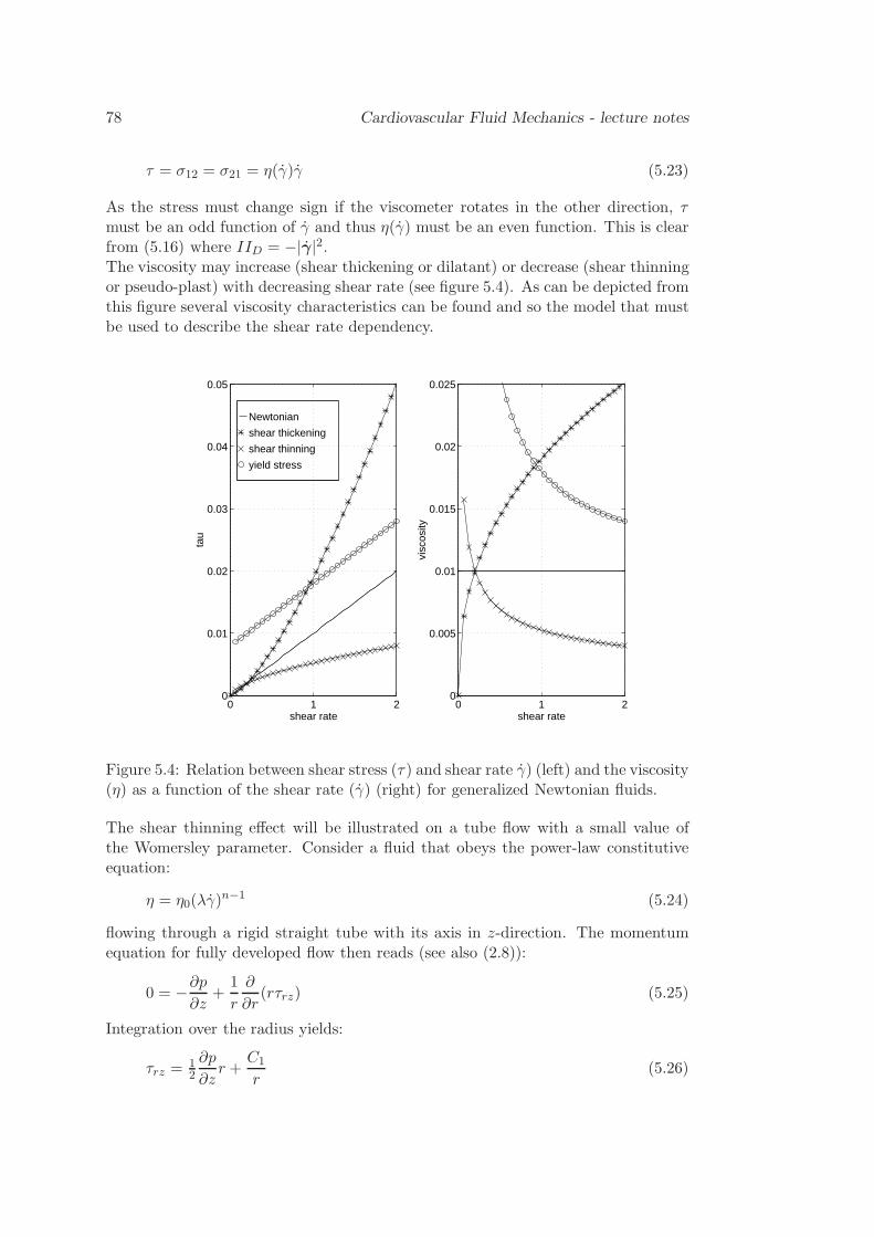
78 Cardiovascular Fluid Mechanics - lecture notes
τ = σ12 = σ21 = η(γ)γ (5.23)
As the stress must change sign if the viscometer rotates in the other direction, τmust be an odd function of γ and thus η(γ) must be an even function. This is clearfrom (5.16) where IID = −|γ|2.The viscosity may increase (shear thickening or dilatant) or decrease (shear thinningor pseudo-plast) with decreasing shear rate (see figure 5.4). As can be depicted fromthis figure several viscosity characteristics can be found and so the model that mustbe used to describe the shear rate dependency.
0 1 20
0.005
0.01
0.015
0.02
0.025
shear rate
visc
osity
Newtonian
shear thickening
shear thinning
yield stress
0 1 20
0.01
0.02
0.03
0.04
0.05
shear rate
tau
Figure 5.4: Relation between shear stress (τ) and shear rate γ) (left) and the viscosity(η) as a function of the shear rate (γ) (right) for generalized Newtonian fluids.
The shear thinning effect will be illustrated on a tube flow with a small value ofthe Womersley parameter. Consider a fluid that obeys the power-law constitutiveequation:
η = η0(λγ)n−1 (5.24)
flowing through a rigid straight tube with its axis in z-direction. The momentumequation for fully developed flow then reads (see also (2.8)):
0 = −∂p∂z
+1
r
∂
∂r(rτrz) (5.25)
Integration over the radius yields:
τrz =12
∂p
∂zr +
C1
r(5.26)
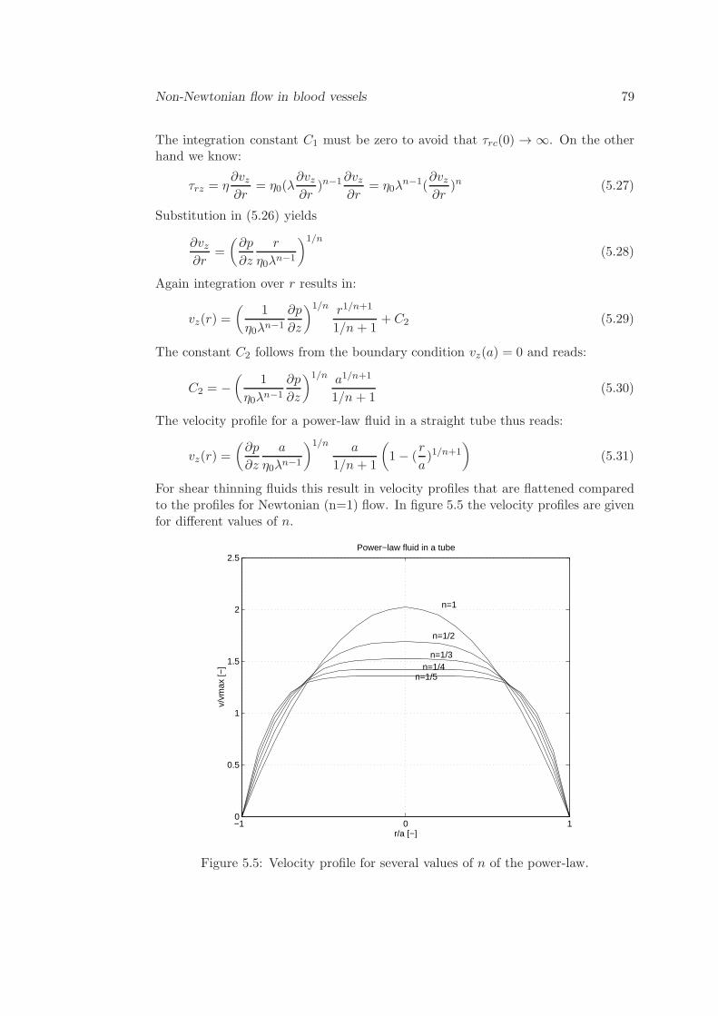
Non-Newtonian flow in blood vessels 79
The integration constant C1 must be zero to avoid that τrc(0) → ∞. On the otherhand we know:
τrz = η∂vz∂r
= η0(λ∂vz∂r
)n−1∂vz∂r
= η0λn−1(
∂vz∂r
)n (5.27)
Substitution in (5.26) yields
∂vz∂r
=
(
∂p
∂z
r
η0λn−1
)1/n
(5.28)
Again integration over r results in:
vz(r) =
(
1
η0λn−1
∂p
∂z
)1/n r1/n+1
1/n + 1+ C2 (5.29)
The constant C2 follows from the boundary condition vz(a) = 0 and reads:
C2 = −(
1
η0λn−1
∂p
∂z
)1/n a1/n+1
1/n + 1(5.30)
The velocity profile for a power-law fluid in a straight tube thus reads:
vz(r) =
(
∂p
∂z
a
η0λn−1
)1/n a
1/n + 1
(
1− (r
a)1/n+1
)
(5.31)
For shear thinning fluids this result in velocity profiles that are flattened comparedto the profiles for Newtonian (n=1) flow. In figure 5.5 the velocity profiles are givenfor different values of n.
−1 0 10
0.5
1
1.5
2
2.5
r/a [−]
v/vm
ax [−
]
Power−law fluid in a tube
n=1
n=1/2
n=1/3n=1/4
n=1/5
Figure 5.5: Velocity profile for several values of n of the power-law.
80 Cardiovascular Fluid Mechanics - lecture notes
5.5 Viscoelastic models
5.5.1 Constitutive equations
If instationary inertia forces can be neglected, for (generalized) Newtonian fluids themomentary stress at a fixed location x, τ(t) is determined by a momentary shearrate γ(t) and is found to be τ(t) = η(IID)γ(t). Generalized Newtonian models candescribe the shear rate dependency of viscosity quite well but can not describe timedependence in the response to deformation. This time dependency is illustratedclearly by the fact that some fluids return to their original form when the appliedstress is released. These fluids do not only have viscous properties (τ(t) = τ(γ(t)))but show also elastic properties (τ(t0, t) = τ(γ(t0, t))). This can be the result ofthe presence of long molecular chains or deformable particles which show an elasticrelaxation after deformation. Note that the elastic response at a fixed location x notonly depends on the time but also on a reference time t0. This, of course, originatesfrom the fact that unlike the shear and strain rate, the shear and strain are definedwith respect to a reference state. The relation between shear and shear rate can beexpressed as:
γ(t) =∂γ(t0, t)
∂t(5.32)
and
γ(t0, t) =
t∫
t0
γ(t′′)dt′′ (5.33)
Constitutive equations for viscoelastic materials are often based on Boltzmann’s su-perposition principle. Each increment in shear δγn at time tn that is experiencedby the material will induce a shear stress τn which will be a function of time butwill be independent of the shear stress that is induced by other increments in shear.So, like infinitesimal strains, also infinitesimal stresses are additive. The time de-pendence of the response to a shear rate increment at time t = tn can be defined bya relaxation function G(t − tn). The relaxation function G(t − tn) mostly is takento be an exponential decay with time constant or characteristic relaxation time λ0according to:
G(t− tn) = G0e−
1
λ0(t−tn)
(5.34)
Following Boltzmann’s superposition principle, the total shear stress at time t thenis given by:
τ(t) =∑
n
δγnG0e−
1
λ0(t−tn)
(5.35)
If we write
δγn(t) =δγ(tn, t)
δtδt ≈ γ(tn)δt (5.36)
Non-Newtonian flow in blood vessels 81
the following expression is found:
τ(t) =
t∫
−∞
γ(t′)G0e−
1
λ0(t−t′)
dt′ (5.37)
Partial integration yields:
τ(t) = G0e−
1
λ0(t−t′)
γ(t, t′)|t−∞ +
t∫
−∞
G0
λ0e−
1
λ0(t−t′)
γ(t, t′)dt′ (5.38)
Here the following definition has been used:
γ(t, t′) =
t∫
t′
γ(t′′)dt′′ (5.39)
Note that γ(t, t′) expresses the shear that is experienced in the period of time betweent′ and t (t′ < t′′ < t) and thus γ(t, t) = 0. As a consequence the first term in (5.38)vanishes. The shear stress then reduces to:
τ(t) =
t∫
−∞
G0
λ0e−
1
λ0(t−t′)
γ(t, t′)dt′ (5.40)
A three-dimensional analog is known as the Lodge integral equation. It provides ageneral integral constitutive equation for viscoelastic fluids (see Macosko, 1994) andreads:
σ(t) =
t∫
−∞
G0
λ0e−
1
λ0(t−t′)
B(t, t′)dt′ (5.41)
In (5.40) the one-dimensional shear stress τ(t) is replaced by the Cauchy stress σ(t)and the shear γ(t, t′) is replaced by the general measure B(t, t′).
A corresponding differential form can be derived by differentiation of the Lodgeintegral equation (5.41). As the upper bound of the integral depends on t theLeibnitz formula is used:
dσ(t)
dt=
G0
λ0e−
1
λ0(t−t′)
B(t, t′)|t−∞+
t∫
−∞
G0
λ0e−
1
λ0(t−t′)
(
− 1
λ0B(t, t′) + B(t, t′)
)
dt′
(5.42)
The first term vanishes for t′ = −∞ and yields (G0/λ0)B(t, t) = (G0/λ0)I for t′ = t.The second part of the second term can be simplified with the aid of relation (A.25).So (5.42) reduces to:
dσ
dt=G0
λ0I − 1
λ0σ +L · σ + σ ·Lc (5.43)
82 Cardiovascular Fluid Mechanics - lecture notes
or:
λ0
(
dσ
dt−L · σ − σ · Lc
)
+ σ = G0I (5.44)
Elimination of the hydrostatic part G0I by substitution of σ = τ +G0I yields:
λ0(τ −L · τ − τ ·Lc −G0L · I −G0I · Lc) + τ = 0 (5.45)
and finally with
L = (∇v)c, (5.46)
L · I + I ·Lc = 2D, (5.47)
η0 = G0λ0 and (5.48)
dτ
dt=∂τ
∂t+ v · ∇τ (5.49)
the differential form of the Lodge integral equation (5.41) is obtained and reads:
λ0
∂τ
∂t+ v · ∇τ − [(∇v)c · τ + τ · (∇v)]
+ τ = 2η0D (5.50)
The term in between the brackets is called the upper convected time derivativeof τ . The constitutive model is called the upper convected Maxwell (UCM) modeland forms the basis of many other models that are proposed in literature.
After introduction of the non-dimensional variables: x∗ = x/L, v∗ = v/V , t∗ = t/θand τ ∗ = τL/η0V a dimensionless form of this equation is given by:
De∂τ
∂t+We [v · ∇τ − (∇v)c · τ − τ · (∇v)] + τ = γ (5.51)
With the dimensionless numbers:
De =λ0θ
Deborah number
We =λ0V
LWeissenberg number
(5.52)
with De the Deborah number defined as the ratio of a characteristic relaxationtime of the fluid λ0 to a characteristic time of the flow θ and We the Weissenbergnumber defined as the ratio of a characteristic relaxation time of the fluid λ0 and acharacteristic time measure of shear rate L/V .
If the Weissenberg number is small a linear viscoelastic (Maxwell) model is foundaccording to:
De∂τ
∂t+ τ = γ (5.53)
Non-Newtonian flow in blood vessels 83
or in dimensionfull form:
λ0∂τ
∂t+ τ = η0γ (5.54)
with η0 the viscosity and λ0 a time constant (for deformation of red blood cellsλ0 = O(0.1s) ). The presence of the time derivative term introduces an elasticcontribution with elastic modulus η0/λ0. For large Deborah numbers this equationyields a constitutive equation for a simple Hookean solid with elastic modulus G =η0/λ0:
τ = Gγ (5.55)
which only holds for small strains γ ≪ 1
Generalized upper convected Maxwell models use more then one relaxation time:
G(t− tn) =K∑
k=0
Gke−
1
λk(t−tk)
(5.56)
Note that for viscoelastic solids at least one time constant λk = ∞ must exist.
5.5.2 Viscometric results
The material behavior of viscoelastic fluids can be illustrated clearly by two experi-mental observations:
Response to a step input in the shear rate :If we define the function S(t) as:
S(t) =
0 t < 0
1 t ≥ 0(5.57)
and a shear rate according to:
γ(t) = γoS(t) (5.58)
The corresponding stress then is found to be:
τ(t) = ηγ0(1− e−t/λ) for t > 0 (5.59)
This indeed consists of two contributions:
elastic : τ = (η/λ)γ0t for t ≪ λ
viscous : τ = ηγ0 for t≫ λ
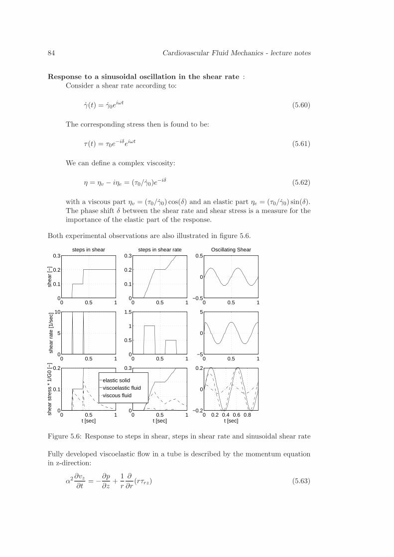
84 Cardiovascular Fluid Mechanics - lecture notes
Response to a sinusoidal oscillation in the shear rate :Consider a shear rate according to:
γ(t) = γ0eiωt (5.60)
The corresponding stress then is found to be:
τ(t) = τ0e−iδeiωt (5.61)
We can define a complex viscosity:
η = ηv − iηe = (τ0/γ0)e−iδ (5.62)
with a viscous part ηv = (τ0/γ0) cos(δ) and an elastic part ηe = (τ0/γ0) sin(δ).The phase shift δ between the shear rate and shear stress is a measure for theimportance of the elastic part of the response.
Both experimental observations are also illustrated in figure 5.6.
0 0.5 10
0.1
0.2
0.3
shea
r [−
]
steps in shear
0 0.5 10
5
10
shea
r ra
te [1
/sec
]
0 0.5 10
0.1
0.2
t [sec]
shea
r st
ress
* 1
/G0
[−]
0 0.5 10
0.1
0.2
0.3steps in shear rate
0 0.5 10
0.5
1
1.5
0 0.5 10
0.1
0.2
0.3
t [sec]
0 0.5 1−0.5
0
0.5Oscillating Shear
0 0.5 1−5
0
5
elastic solid viscoelastic fluidviscous fluid
0 0.2 0.4 0.6 0.8−0.2
0
0.2
t [sec]
Figure 5.6: Response to steps in shear, steps in shear rate and sinusoidal shear rate
Fully developed viscoelastic flow in a tube is described by the momentum equationin z-direction:
α2 ∂vz∂t
= −∂p∂z
+1
r
∂
∂r(rτrz) (5.63)
Non-Newtonian flow in blood vessels 85
With the aid of:
v =
00vz
∇v =
0 0 γ0 0 00 0 0
(5.64)
with γ = ∂vz∂r . It can easily be verified that v ·∇τ = 0 and that the upper convected
Maxwell model reduces to:
De ∂∂t
τrr τrφ τrzτφr τφφ τφzτzr τzφ τzz
−We
0 0 τrrγ0 0 τφrγτrrγ τrφγ 2τzrγ
+
+
τrr τrφ τrzτφr τφφ τφzτzr τzφ τzz
=
0 0 γ0 0 0γ 0 0
(5.65)
Making use of symmetry of τ and assuming a stress free initial condition, this yields:
De∂τrz∂t
+ τrz = γ (5.66)
and
De∂τzz∂t
− 2Weγτrz + τzz = 0 (5.67)
We search for harmonic solutions:
vz(r) = vz(r)eiωt,
∂p
∂z=∂p
∂zeiωt, τrz(r) = τrz(r)e
iωt (5.68)
Equation (5.66) in dimensionfull form then can be solved and yields the followingrelation between the shear stress and the shear rate:
τrz =η
1 + iωλγ (5.69)
This shows that the solution of (5.63) for viscoelastic flow is exactly the same asthe one for Newtonian flow except for the viscosity that in the viscoelastic case is acomplex function according to:
ν∗ =ν
1 + iωλ(5.70)
The two dimensionless parameters thus are:
De = ωλ (5.71)
and
α∗ = a
√
ω(1 + iDe)
ν= (1 + iDe)1/2α (5.72)
The solution of the velocity field will again be (see (2.22)):
vz(r) =i
ρω
∂p
∂z
[
1− J0(i3/2α∗r/a)
J0(i3/2α∗)
]
(5.73)
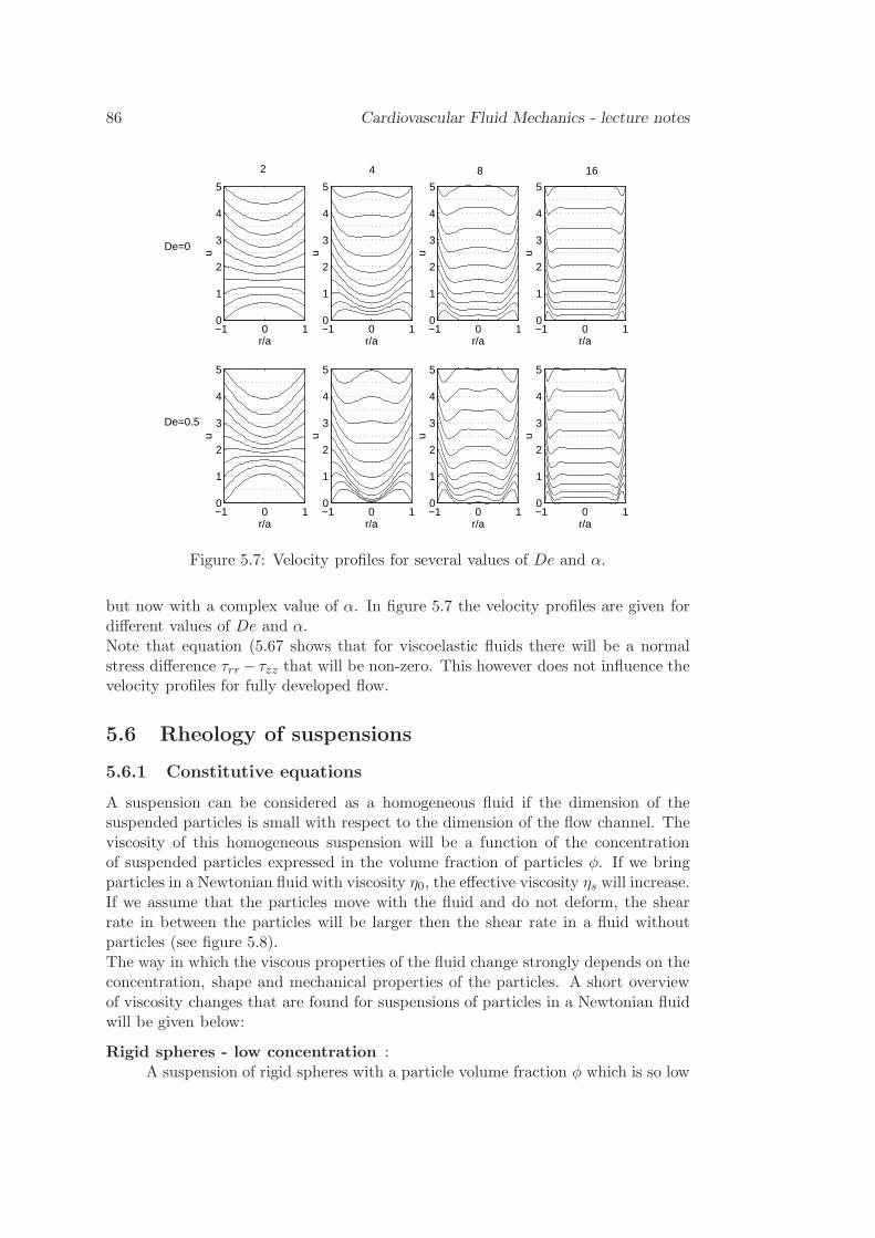
86 Cardiovascular Fluid Mechanics - lecture notes
−1 0 10
1
2
3
4
5
u
r/a−1 0 10
1
2
3
4
5
u
r/a−1 0 10
1
2
3
4
5
u
r/a−1 0 10
1
2
3
4
5
u
r/a
−1 0 10
1
2
3
4
5
u
r/a−1 0 10
1
2
3
4
5
u
r/a−1 0 10
1
2
3
4
5
u
r/a−1 0 10
1
2
3
4
5
ur/a
2 4 8 16
De=0
De=0.5
Figure 5.7: Velocity profiles for several values of De and α.
but now with a complex value of α. In figure 5.7 the velocity profiles are given fordifferent values of De and α.Note that equation (5.67 shows that for viscoelastic fluids there will be a normalstress difference τrr − τzz that will be non-zero. This however does not influence thevelocity profiles for fully developed flow.
5.6 Rheology of suspensions
5.6.1 Constitutive equations
A suspension can be considered as a homogeneous fluid if the dimension of thesuspended particles is small with respect to the dimension of the flow channel. Theviscosity of this homogeneous suspension will be a function of the concentrationof suspended particles expressed in the volume fraction of particles φ. If we bringparticles in a Newtonian fluid with viscosity η0, the effective viscosity ηs will increase.If we assume that the particles move with the fluid and do not deform, the shearrate in between the particles will be larger then the shear rate in a fluid withoutparticles (see figure 5.8).The way in which the viscous properties of the fluid change strongly depends on theconcentration, shape and mechanical properties of the particles. A short overviewof viscosity changes that are found for suspensions of particles in a Newtonian fluidwill be given below:
Rigid spheres - low concentration :A suspension of rigid spheres with a particle volume fraction φ which is so low
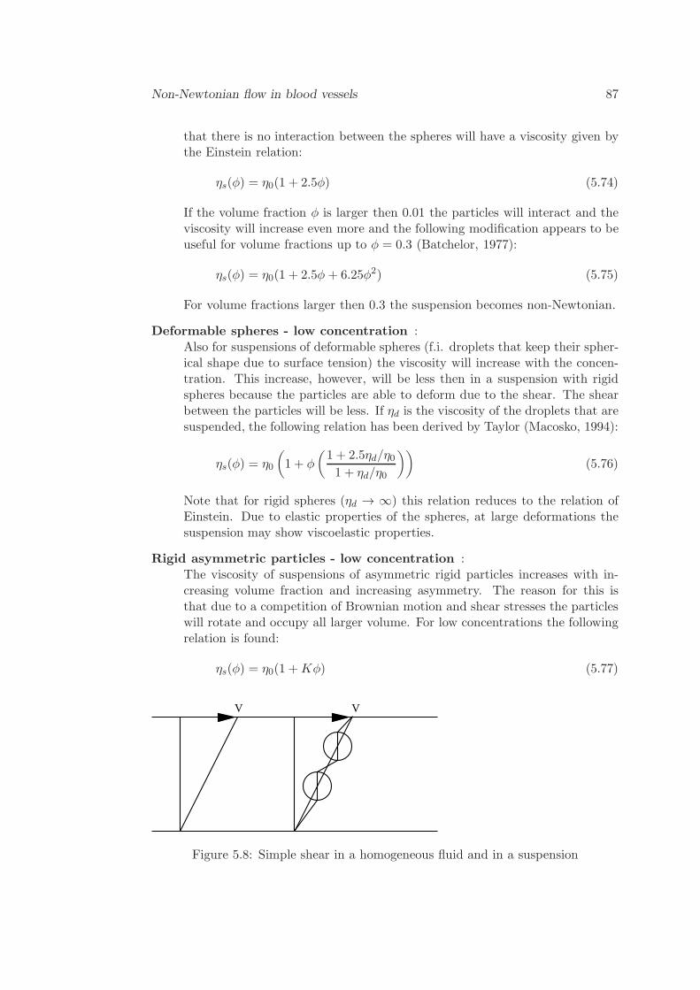
Non-Newtonian flow in blood vessels 87
that there is no interaction between the spheres will have a viscosity given bythe Einstein relation:
ηs(φ) = η0(1 + 2.5φ) (5.74)
If the volume fraction φ is larger then 0.01 the particles will interact and theviscosity will increase even more and the following modification appears to beuseful for volume fractions up to φ = 0.3 (Batchelor, 1977):
ηs(φ) = η0(1 + 2.5φ + 6.25φ2) (5.75)
For volume fractions larger then 0.3 the suspension becomes non-Newtonian.
Deformable spheres - low concentration :Also for suspensions of deformable spheres (f.i. droplets that keep their spher-ical shape due to surface tension) the viscosity will increase with the concen-tration. This increase, however, will be less then in a suspension with rigidspheres because the particles are able to deform due to the shear. The shearbetween the particles will be less. If ηd is the viscosity of the droplets that aresuspended, the following relation has been derived by Taylor (Macosko, 1994):
ηs(φ) = η0
(
1 + φ
(
1 + 2.5ηd/η01 + ηd/η0
))
(5.76)
Note that for rigid spheres (ηd → ∞) this relation reduces to the relation ofEinstein. Due to elastic properties of the spheres, at large deformations thesuspension may show viscoelastic properties.
Rigid asymmetric particles - low concentration :The viscosity of suspensions of asymmetric rigid particles increases with in-creasing volume fraction and increasing asymmetry. The reason for this isthat due to a competition of Brownian motion and shear stresses the particleswill rotate and occupy all larger volume. For low concentrations the followingrelation is found:
ηs(φ) = η0(1 +Kφ) (5.77)
V V
Figure 5.8: Simple shear in a homogeneous fluid and in a suspension
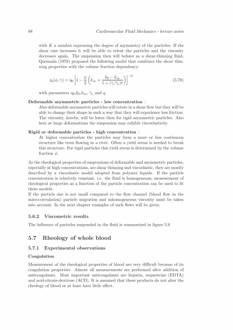
88 Cardiovascular Fluid Mechanics - lecture notes
with K a number expressing the degree of asymmetry of the particles. If theshear rate increases it will be able to orient the particles and the viscositydecreases again. The suspension then will behave as a shear-thinning fluid.Quemada (1978) proposed the following model that combines the shear thin-ning properties with the volume fraction dependency:
ηs(φ, γ) = η0
[
1− φ
2
(
k∞ +k0 − k∞
1 + (γ/γc)q
)]−2
(5.78)
with parameters η0,k0,k∞, γc and q.
Deformable asymmetric particles - low concentration :Also deformable asymmetric particles will rotate in a shear flow but they will beable to change their shape in such a way that they will experience less friction.The viscosity, hereby, will be lower then for rigid asymmetric particles. Alsohere at large deformations the suspension may exhibit viscoelasticity.
Rigid or deformable particles - high concentration :At higher concentration the particles may form a more or less continuousstructure like trees flowing in a river. Often a yield stress is needed to breakthis structure. For rigid particles this yield stress is determined by the volumefraction φ.
As the rheological properties of suspensions of deformable and asymmetric particles,especially at high concentrations, are shear thinning and viscoelastic, they are mostlydescribed by a viscoelastic model adopted from polymer liquids. If the particleconcentration is relatively constant, i.e. the fluid is homogeneous, measurement ofrheological properties as a function of the particle concentration can be used to fitthese models.
If the particle size is not small compared to the flow channel (blood flow in themicro-circulation) particle migration and inhomogeneous viscosity must be takeninto account. In the next chapter examples of such flows will be given.
5.6.2 Viscometric results
The influence of particles suspended in the fluid is summarized in figure 5.9
5.7 Rheology of whole blood
5.7.1 Experimental observations
Coagulation
Measurement of the rheological properties of blood are very difficult because of itscoagulation properties. Almost all measurements are performed after addition ofanticoagulants. Most important anticoagulants are heparin, sequestrine (EDTA)and acid-citrate-dextrose (ACD). It is assumed that these products do not alter therheology of blood or at least have little effect.
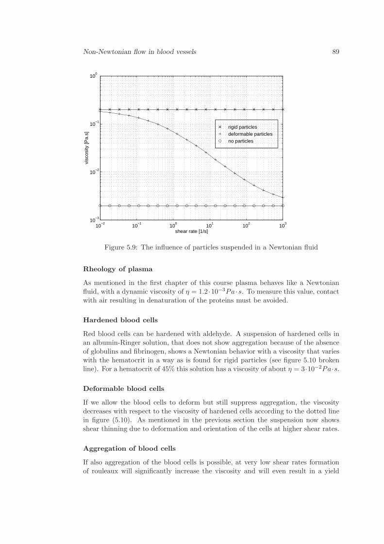
Non-Newtonian flow in blood vessels 89
rigid particles deformable particlesno particles
10−2
10−1
100
101
102
103
10−3
10−2
10−1
100
shear rate [1/s]
visc
osity
[Pa.
s]
Figure 5.9: The influence of particles suspended in a Newtonian fluid
Rheology of plasma
As mentioned in the first chapter of this course plasma behaves like a Newtonianfluid, with a dynamic viscosity of η = 1.2 ·10−3Pa ·s. To measure this value, contactwith air resulting in denaturation of the proteins must be avoided.
Hardened blood cells
Red blood cells can be hardened with aldehyde. A suspension of hardened cells inan albumin-Ringer solution, that does not show aggregation because of the absenceof globulins and fibrinogen, shows a Newtonian behavior with a viscosity that varieswith the hematocrit in a way as is found for rigid particles (see figure 5.10 brokenline). For a hematocrit of 45% this solution has a viscosity of about η = 3·10−2Pa·s.
Deformable blood cells
If we allow the blood cells to deform but still suppress aggregation, the viscositydecreases with respect to the viscosity of hardened cells according to the dotted linein figure (5.10). As mentioned in the previous section the suspension now showsshear thinning due to deformation and orientation of the cells at higher shear rates.
Aggregation of blood cells
If also aggregation of the blood cells is possible, at very low shear rates formationof rouleaux will significantly increase the viscosity and will even result in a yield
90 Cardiovascular Fluid Mechanics - lecture notes
stress with an order of magnitude equal to 1− 5 · 10−3Pa. At higher shear rates therouleaux will break down and a behavior as is found for the albumin-Ringer solutionwill be found.
103100101102 deformation
visc
osi
ty[Pa:s]
shear rate [1=s] 102101100101erythrocytes in Ringer
hardened erythrocytes
normal blood
aggregation
Figure 5.10: Viscosity in steady shear of normal blood, blood with hardened ery-throcytes (no deformation) and blood in a Ringer solution (no aggregation). From(Chien et al., 1969).
Viscoelastic properties of blood
The deformability and the orientation of the rouleaux and the individual erythro-cytes lead to the viscoelastic behavior of blood. They provide a mean of storing en-ergy during flow. Thurston (1973) investigated the viscoelastic properties of bloodin the linear viscoelastic regime and measured a significant elastic component inoscillatory blood flow (figure 5.11).
McMillan et al. (1987) investigated the transient properties of blood in viscometricflow. They measured the shear stress generated by blood, subjected to a number ofsequential steps in the shear rate. The overshoot in the shear stress was attributedto orientation of erythrocytes and aggregates. The delayed relaxation of the shearstress can be related to the viscoelastic properties of blood. The transient data canbe used to compute time scales for the formation and break-up of rouleaux.
5.7.2 Constitutive equations
The constitutive equation (5.50) is a relation between τ and γ. More complexrelations can be obtained using more then one time constant and superposition ofsimple models. Also non-linear relations letting e.g. γ = γ(τ · τ ), η = η(γ) or
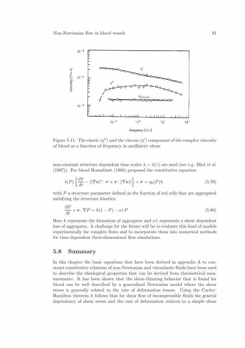
Non-Newtonian flow in blood vessels 91
103102vi
sco
sity
[Pa:s]100
101101 0plasma 101
frequency [Hz]
102000
Figure 5.11: The elastic (η′′) and the viscous (η′) component of the complex viscosityof blood as a function of frequency in oscillatory shear.
non-constant structure dependent time scales λ = λ(γ) are used (see e.g. Bird et al.
(1987)). For blood Rosenblatt (1988) proposed the constitutive equation:
λ(P )
dτ
dt− [(∇v)c · τ + τ · (∇v)]
+ τ = η0(P )γ (5.79)
with P a structure parameter defined as the fraction of red cells that are aggregatedsatisfying the structure kinetics:
∂P
∂t+ v · ∇P = k(1− P )− αγP (5.80)
Here k represents the formation of aggregates and αγ represents a shear dependentloss of aggregates. A challenge for the future will be to evaluate this kind of modelsexperimentally for complex flows and to incorporate them into numerical methodsfor time-dependent three-dimensional flow simulations.
5.8 Summary
In this chapter the basic equations that have been derived in appendix A to con-struct constitutive relations of non-Newtonian and viscoelastic fluids have been usedto describe the rheological properties that can be derived from rheometrical mea-surements. It has been shown that the shear-thinning behavior that is found forblood can be well described by a generalized Newtonian model where the shearstress is generally related to the rate of deformation tensor. Using the Cayley-Hamilton theorem it follows that for shear flow of incompressible fluids the generaldependency of shear stress and the rate of deformation reduces to a simple shear
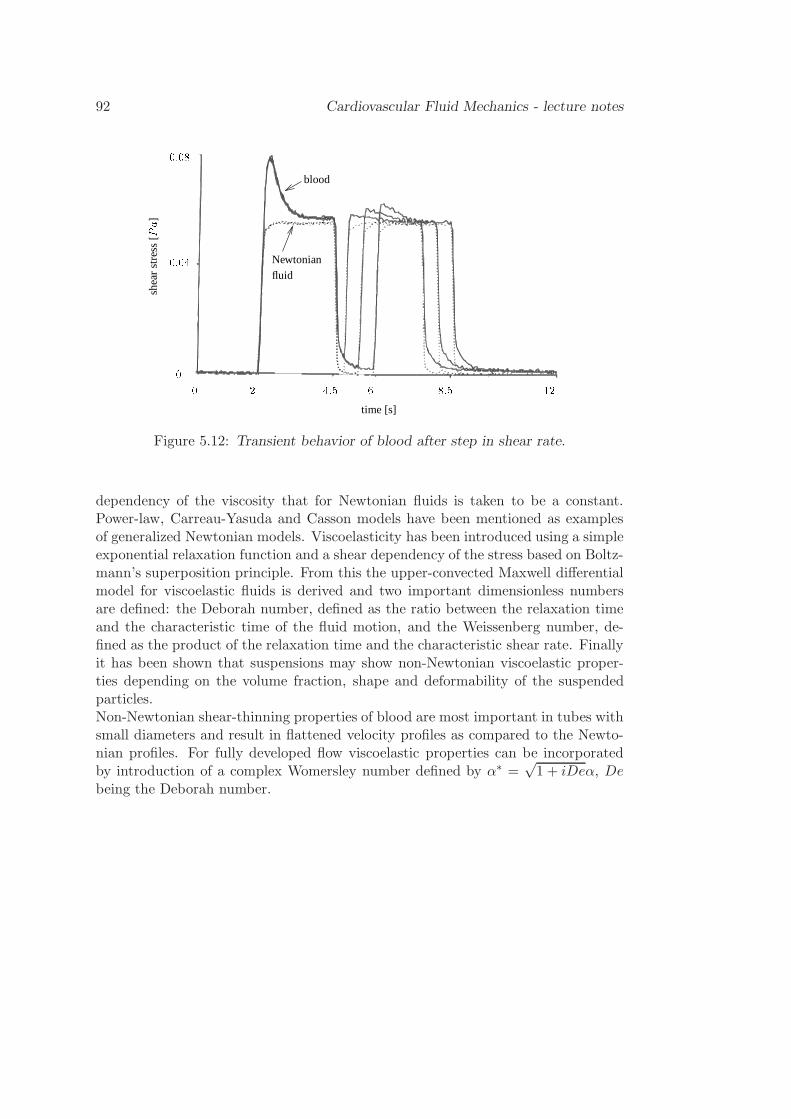
92 Cardiovascular Fluid Mechanics - lecture notes
00:040:08
shea
rst
ress
[Pa]0 2
blood
4:5 6 8:5 12time [s]
Newtonianfluid
Figure 5.12: Transient behavior of blood after step in shear rate.
dependency of the viscosity that for Newtonian fluids is taken to be a constant.Power-law, Carreau-Yasuda and Casson models have been mentioned as examplesof generalized Newtonian models. Viscoelasticity has been introduced using a simpleexponential relaxation function and a shear dependency of the stress based on Boltz-mann’s superposition principle. From this the upper-convected Maxwell differentialmodel for viscoelastic fluids is derived and two important dimensionless numbersare defined: the Deborah number, defined as the ratio between the relaxation timeand the characteristic time of the fluid motion, and the Weissenberg number, de-fined as the product of the relaxation time and the characteristic shear rate. Finallyit has been shown that suspensions may show non-Newtonian viscoelastic proper-ties depending on the volume fraction, shape and deformability of the suspendedparticles.Non-Newtonian shear-thinning properties of blood are most important in tubes withsmall diameters and result in flattened velocity profiles as compared to the Newto-nian profiles. For fully developed flow viscoelastic properties can be incorporatedby introduction of a complex Womersley number defined by α∗ =
√1 + iDeα, De
being the Deborah number.
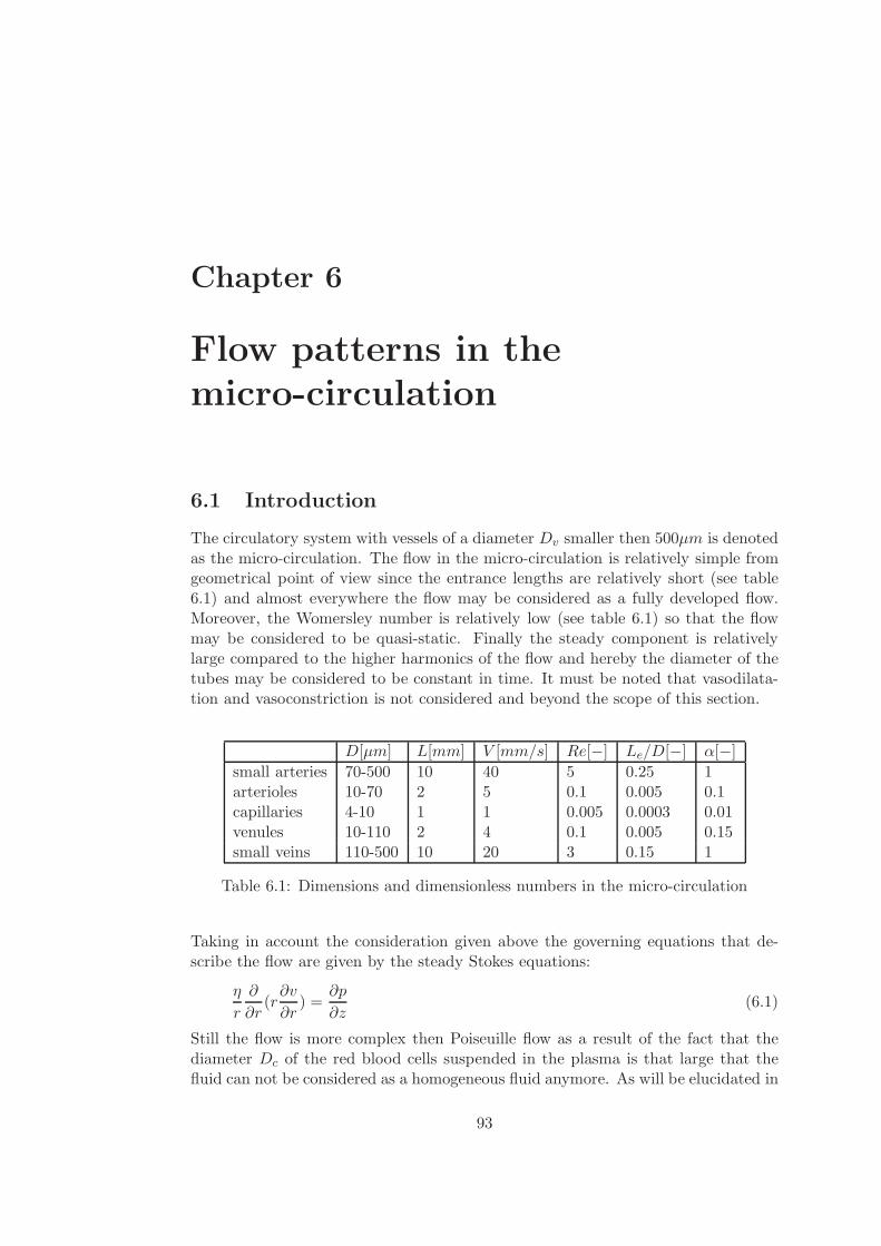
Chapter 6
Flow patterns in the
micro-circulation
6.1 Introduction
The circulatory system with vessels of a diameter Dv smaller then 500µm is denotedas the micro-circulation. The flow in the micro-circulation is relatively simple fromgeometrical point of view since the entrance lengths are relatively short (see table6.1) and almost everywhere the flow may be considered as a fully developed flow.Moreover, the Womersley number is relatively low (see table 6.1) so that the flowmay be considered to be quasi-static. Finally the steady component is relativelylarge compared to the higher harmonics of the flow and hereby the diameter of thetubes may be considered to be constant in time. It must be noted that vasodilata-tion and vasoconstriction is not considered and beyond the scope of this section.
D[µm] L[mm] V [mm/s] Re[−] Le/D[−] α[−]
small arteries 70-500 10 40 5 0.25 1arterioles 10-70 2 5 0.1 0.005 0.1capillaries 4-10 1 1 0.005 0.0003 0.01venules 10-110 2 4 0.1 0.005 0.15small veins 110-500 10 20 3 0.15 1
Table 6.1: Dimensions and dimensionless numbers in the micro-circulation
Taking in account the consideration given above the governing equations that de-scribe the flow are given by the steady Stokes equations:
η
r
∂
∂r(r∂v
∂r) =
∂p
∂z(6.1)
Still the flow is more complex then Poiseuille flow as a result of the fact that thediameter Dc of the red blood cells suspended in the plasma is that large that thefluid can not be considered as a homogeneous fluid anymore. As will be elucidated in
93
94 Cardiovascular Fluid Mechanics - lecture notes
the next sections, the flow in the micro-circulation can be divided into three regimes:small arteries and small veins (Dv > 2Dc), arterioles and venules (Dc < Dv < 2Dc)and capillaries (Dv < Dc).
6.2 Flow in small arteries and small veins: Dv > 2Dc
If the ratio of the vessel diameterDv and the cell diameterDc is large, we may assumethat the fluid in the core of the vessel is a homogeneous suspension of particles. Theconcentration of the particles in the core is constant and hereby the core will havea viscosity ηc. At the vessel wall, however, the concentration of particles will belower due to the fact that they can not penetrate through the wall. A possibleconcentration profile then will look like the one depicted in figure 6.1. At a distancesmaller then half the cell diameter 1
2Dc the concentration is assumed to be zeroc(a − 1
2Dc < r < a) = 0. The concentration in the core is assumed to be constantc(r < a− 1
2Dc) = cc. With the definition ac = a− 12Dc this yields:
c =
cc 0 < r < ac0 ac < r < a
(6.2)
The viscosity then will be also a function of the radius according to:
η =
ηc 0 < r < acηp ac < r < a
(6.3)
6.3 Velocity profiles
The velocity profiles can be computed from the momentum equations:
∂
∂r
(
rηc∂v
∂r
)
= r∂p
∂z0 < r < ac
∂
∂r
(
rηp∂v
∂r
)
= r∂p
∂zac < r < a
(6.4)
Integration from 0 to r assuming the stress to be constant over the interface r = ac,again integration from 0 to r assuming the velocity to be constant over the interfaceand substitution of the boundary conditions at r = a yields:
v(r) =r2 − a2c4ηc
∂p
∂z+a2c − a2
4ηp
∂p
∂z0 < r < ac
v(r) =r2 − a2
4ηp
∂p
∂zac < r < a
(6.5)
or with the dimensionless radius ξ = r/a and the dimensionless core diameter λc =ac/a:
v(ξ) = − a2
4ηc(λ2c − ξ2)
∂p
∂z+
a2
4ηp(λ2c − 1)
∂p
∂z0 < ξ < λc
v(ξ) = − a2
4ηp(1− ξ2)
∂p
∂zλc < ξ < 1
(6.6)
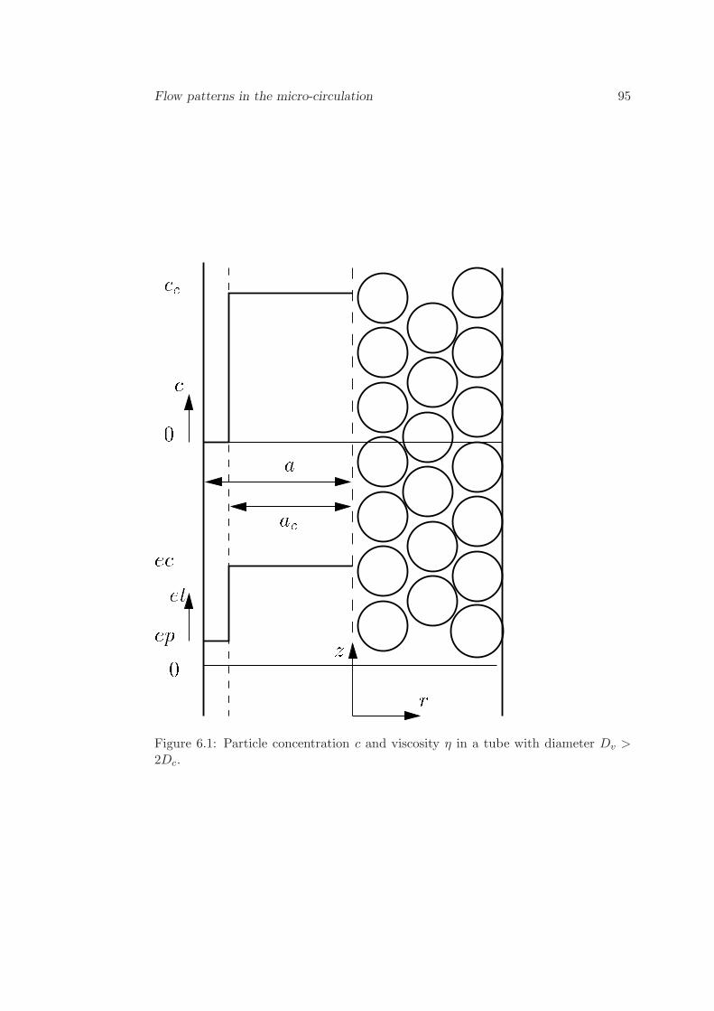
Flow patterns in the micro-circulation 95
acc0epecetc ac z r0
Figure 6.1: Particle concentration c and viscosity η in a tube with diameter Dv >2Dc.
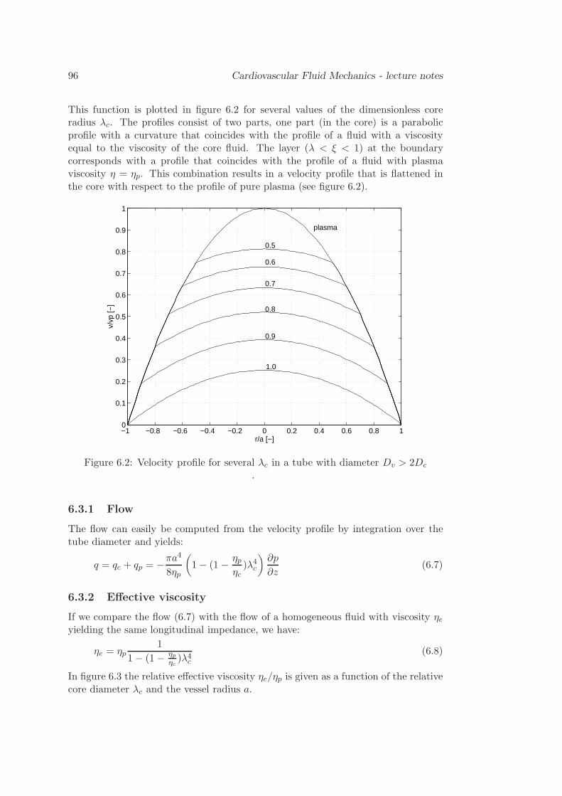
96 Cardiovascular Fluid Mechanics - lecture notes
This function is plotted in figure 6.2 for several values of the dimensionless coreradius λc. The profiles consist of two parts, one part (in the core) is a parabolicprofile with a curvature that coincides with the profile of a fluid with a viscosityequal to the viscosity of the core fluid. The layer (λ < ξ < 1) at the boundarycorresponds with a profile that coincides with the profile of a fluid with plasmaviscosity η = ηp. This combination results in a velocity profile that is flattened inthe core with respect to the profile of pure plasma (see figure 6.2).
−1 −0.8 −0.6 −0.4 −0.2 0 0.2 0.4 0.6 0.8 10
0.1
0.2
0.3
0.4
0.5
0.6
0.7
0.8
0.9
1
r/a [−]
v/vp
[−]
plasma
0.5
0.6
0.7
0.8
0.9
1.0
Figure 6.2: Velocity profile for several λc in a tube with diameter Dv > 2Dc
.
6.3.1 Flow
The flow can easily be computed from the velocity profile by integration over thetube diameter and yields:
q = qc + qp = −πa4
8ηp
(
1− (1− ηpηc
)λ4c
)
∂p
∂z(6.7)
6.3.2 Effective viscosity
If we compare the flow (6.7) with the flow of a homogeneous fluid with viscosity ηeyielding the same longitudinal impedance, we have:
ηe = ηp1
1− (1− ηpηc)λ4c
(6.8)
In figure 6.3 the relative effective viscosity ηe/ηp is given as a function of the relativecore diameter λc and the vessel radius a.
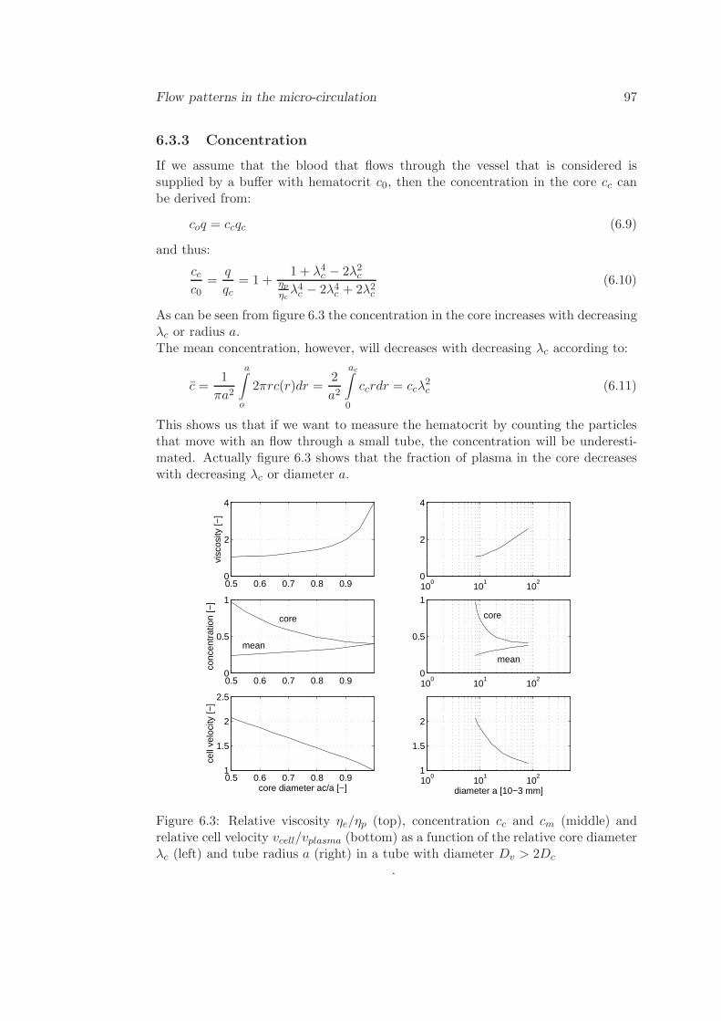
Flow patterns in the micro-circulation 97
6.3.3 Concentration
If we assume that the blood that flows through the vessel that is considered issupplied by a buffer with hematocrit c0, then the concentration in the core cc canbe derived from:
coq = ccqc (6.9)
and thus:
ccc0
=q
qc= 1 +
1 + λ4c − 2λ2cηpηcλ4c − 2λ4c + 2λ2c
(6.10)
As can be seen from figure 6.3 the concentration in the core increases with decreasingλc or radius a.The mean concentration, however, will decreases with decreasing λc according to:
c =1
πa2
a∫
o
2πrc(r)dr =2
a2
ac∫
0
ccrdr = ccλ2c (6.11)
This shows us that if we want to measure the hematocrit by counting the particlesthat move with an flow through a small tube, the concentration will be underesti-mated. Actually figure 6.3 shows that the fraction of plasma in the core decreaseswith decreasing λc or diameter a.
0.5 0.6 0.7 0.8 0.90
2
4
visc
osity
[−]
100
101
102
0
2
4
0.5 0.6 0.7 0.8 0.90
0.5
1
conc
entr
atio
n [−
]
0.5 0.6 0.7 0.8 0.91
1.5
2
2.5
core diameter ac/a [−]
cell
velo
city
[−]
100
101
102
0
0.5
1
100
101
102
1
1.5
2
diameter a [10−3 mm]
core core
mean
mean
Figure 6.3: Relative viscosity ηe/ηp (top), concentration cc and cm (middle) andrelative cell velocity vcell/vplasma (bottom) as a function of the relative core diameterλc (left) and tube radius a (right) in a tube with diameter Dv > 2Dc
.
98 Cardiovascular Fluid Mechanics - lecture notes
6.3.4 Cell velocity
In order to determine the velocity of the cells relative to the velocity of the sur-rounding plasma we compute the volume flow of cells:
qcell = 2π
a∫
0
vcrdr = vcellcπa2 (6.12)
The volume flow of plasma is:
qplasma = 2π
a∫
0
v(1 − c)dr = vplasma(1− c)πa2 (6.13)
The ratio between both flows is given by the hematocrit c0 according to:
qplasma
qcell=
1− c0c0
(6.14)
This yields (see also figure 6.3):
vcellvplasma
=c0
1− c0
1− c
c(6.15)
6.4 Flow in arterioles and venules : Dc < Dv < 2Dc
If the vessel diameter is in between 1 and 2 times the cell diameter, the cells haveto move in a single train (see figure 6.4). The velocity in the core hereby will beconstant. Similar to what has been shown in the previous section for vessels with adiameter larger then 2Dc the velocity, flow, effective viscosity, effective concentrationand cell velocity can be computed. As the central core behaves as a solid cylinder,it can be seen as a fluid with an infinite viscosity. The equations that are derivedin the previous section can be simplified for the case that ηc → ∞. Note thatin the previous section with decreasing diameter the influence of the plasma layerincreased. In this section, for smaller diameters, decreasing the diameter will alsodecrease the influence of the plasma layer.
6.4.1 Velocity profiles
The velocity can be derived from (6.6) using ηc → ∞.
v(ξ) =a2
4ηp(λ2c − 1)
∂p
∂z0 < ξ < λc
v(ξ) = − a2
4ηp(1− ξ2)
∂p
∂zλc < ξ < 1
(6.16)
6.4.2 Flow
The flow again can be derived from the velocity profiles are can be computed from(6.7) using ηc → ∞.
q = qc + qp = −πa4
8ηp
(
1− λ4c
) ∂p
∂z(6.17)
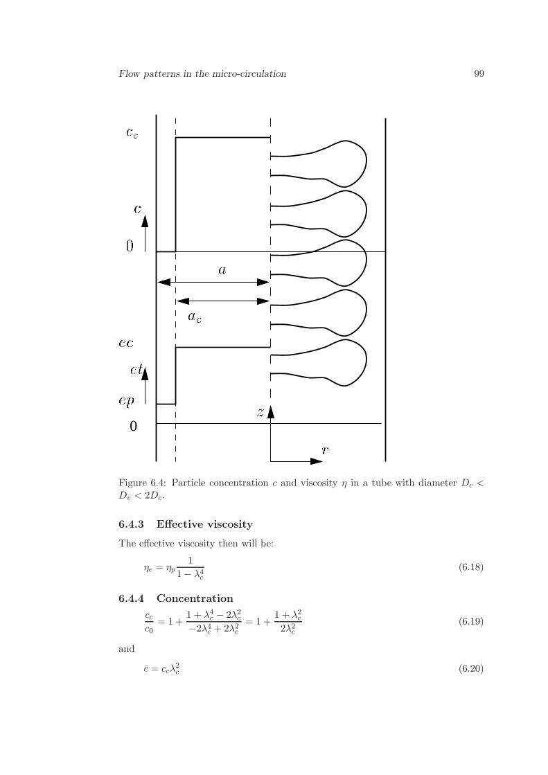
Flow patterns in the micro-circulation 99
0
acc0epecetc
z racFigure 6.4: Particle concentration c and viscosity η in a tube with diameter Dc <Dv < 2Dc.
6.4.3 Effective viscosity
The effective viscosity then will be:
ηe = ηp1
1− λ4c(6.18)
6.4.4 Concentration
ccc0
= 1 +1 + λ4c − 2λ2c−2λ4c + 2λ2c
= 1 +1 + λ2c2λ2c
(6.19)
and
c = ccλ2c (6.20)
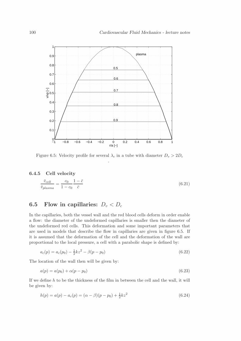
100 Cardiovascular Fluid Mechanics - lecture notes
−1 −0.8 −0.6 −0.4 −0.2 0 0.2 0.4 0.6 0.8 10
0.1
0.2
0.3
0.4
0.5
0.6
0.7
0.8
0.9
1
r/a [−]
v/vp
[−]
plasma
0.5
0.6
0.7
0.8
0.9
Figure 6.5: Velocity profile for several λc in a tube with diameter Dv > 2Dc
.
6.4.5 Cell velocity
vcellvplasma
=c0
1− c0
1− c
c(6.21)
6.5 Flow in capillaries: Dv < Dc
In the capillaries, both the vessel wall and the red blood cells deform in order enablea flow: the diameter of the undeformed capillaries is smaller then the diameter ofthe undeformed red cells. This deformation and some important parameters thatare used in models that describe the flow in capillaries are given in figure 6.5. Ifit is assumed that the deformation of the cell and the deformation of the wall areproportional to the local pressure, a cell with a parabolic shape is defined by:
ac(p) = ac(p0)− 12kz
2 − β(p− p0) (6.22)
The location of the wall then will be given by:
a(p) = a(p0) + α(p − p0) (6.23)
If we define h to be the thickness of the film in between the cell and the wall, it willbe given by:
h(p) = a(p)− ac(p) = (α− β)(p − p0) +12kz
2 (6.24)
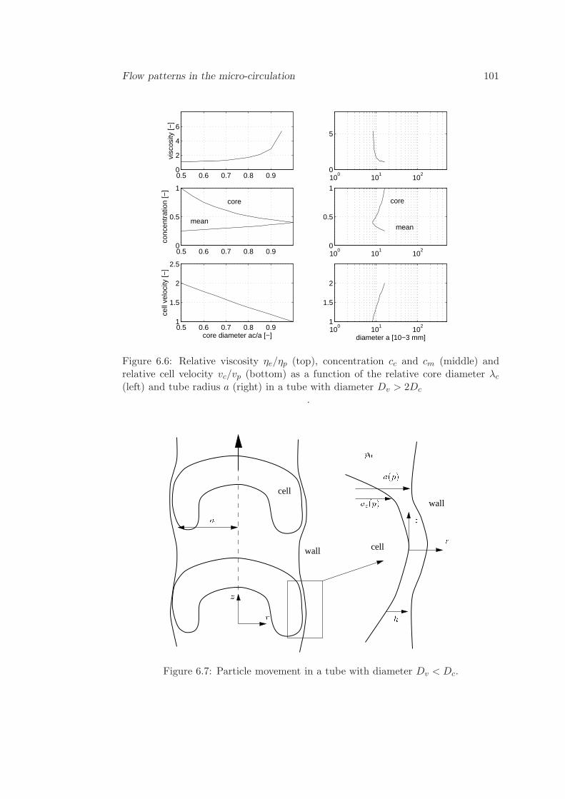
Flow patterns in the micro-circulation 101
0.5 0.6 0.7 0.8 0.90
2
4
6
visc
osity
[−]
100
101
102
0
5
0.5 0.6 0.7 0.8 0.91
1.5
2
2.5
core diameter ac/a [−]
cell
velo
city
[−]
0.5 0.6 0.7 0.8 0.90
0.5
1
conc
entr
atio
n [−
]
100
101
102
0
0.5
1
100
101
102
1
1.5
2
diameter a [10−3 mm]
core core
meanmean
Figure 6.6: Relative viscosity ηe/ηp (top), concentration cc and cm (middle) andrelative cell velocity vc/vp (bottom) as a function of the relative core diameter λc(left) and tube radius a (right) in a tube with diameter Dv > 2Dc
.
a z rcell
wall hcell
wallrza(p)ac(p)p0Figure 6.7: Particle movement in a tube with diameter Dv < Dc.
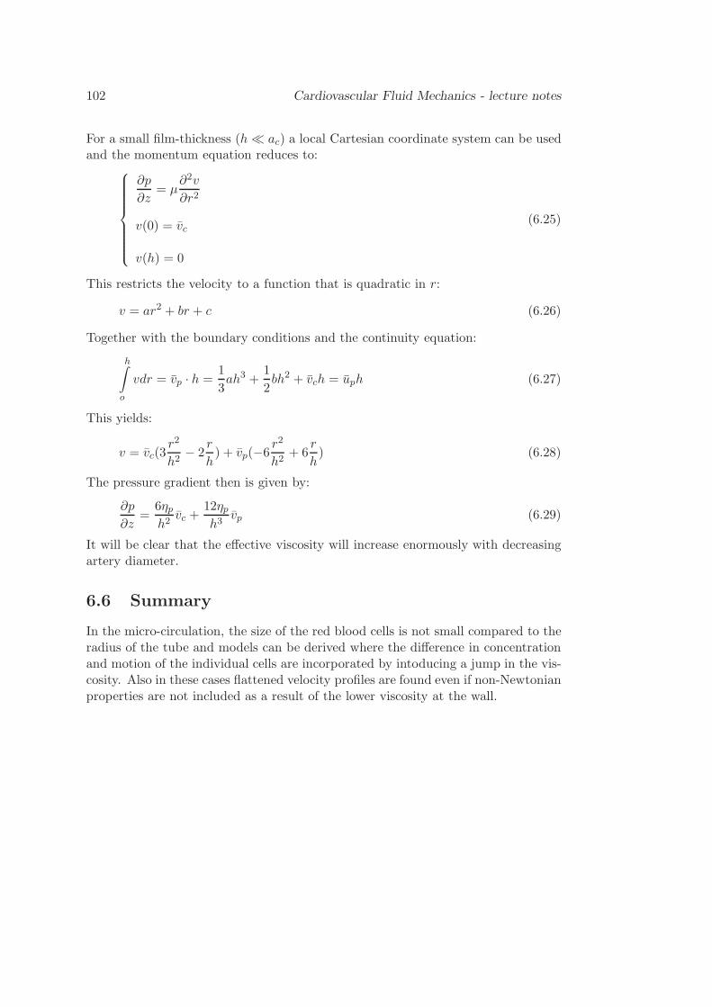
102 Cardiovascular Fluid Mechanics - lecture notes
For a small film-thickness (h≪ ac) a local Cartesian coordinate system can be usedand the momentum equation reduces to:
∂p
∂z= µ
∂2v
∂r2
v(0) = vc
v(h) = 0
(6.25)
This restricts the velocity to a function that is quadratic in r:
v = ar2 + br + c (6.26)
Together with the boundary conditions and the continuity equation:
h∫
o
vdr = vp · h =1
3ah3 +
1
2bh2 + vch = uph (6.27)
This yields:
v = vc(3r2
h2− 2
r
h) + vp(−6
r2
h2+ 6
r
h) (6.28)
The pressure gradient then is given by:
∂p
∂z=
6ηph2
vc +12ηph3
vp (6.29)
It will be clear that the effective viscosity will increase enormously with decreasingartery diameter.
6.6 Summary
In the micro-circulation, the size of the red blood cells is not small compared to theradius of the tube and models can be derived where the difference in concentrationand motion of the individual cells are incorporated by intoducing a jump in the vis-cosity. Also in these cases flattened velocity profiles are found even if non-Newtonianproperties are not included as a result of the lower viscosity at the wall.
Appendix A
Basic equations
A.1 Introduction
In this section the equations that govern the deformation of a solid and motion of afluid will be given. For isothermal systems these can be derived from the equationsof conservation of mass and momentum. For non-isothermal systems the motion isalso determined by the conservation of energy. Using limiting values of the non-dimensional parameters, simplifications of these equations can be derived that willbe used in subsequent chapters. For a detailed treatment of general fluid dynamicsand boundary layer flow the reader is referred to Batchelor (1967) and Schlichting(1960) respectively. More details concerning non-Newtonian and viscoelastic fluidflow can be found in chapter 5 and in Bird et al. (1960, 1987).
103
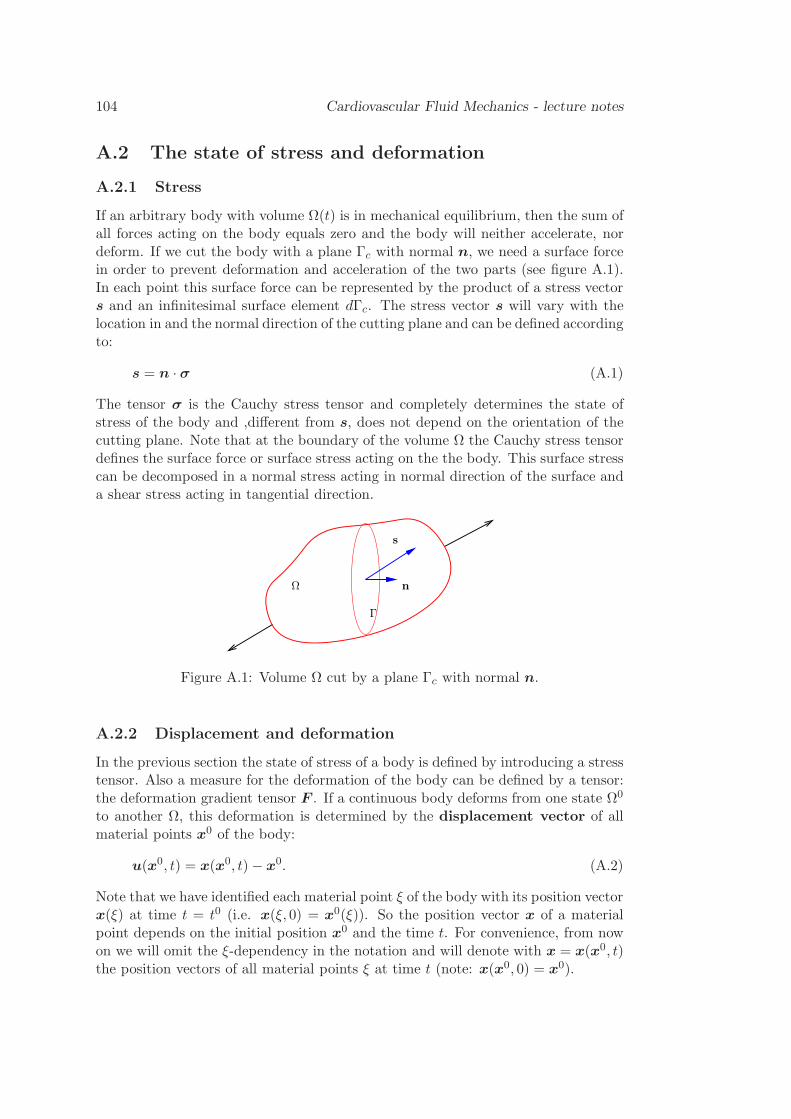
104 Cardiovascular Fluid Mechanics - lecture notes
A.2 The state of stress and deformation
A.2.1 Stress
If an arbitrary body with volume Ω(t) is in mechanical equilibrium, then the sum ofall forces acting on the body equals zero and the body will neither accelerate, nordeform. If we cut the body with a plane Γc with normal n, we need a surface forcein order to prevent deformation and acceleration of the two parts (see figure A.1).In each point this surface force can be represented by the product of a stress vectors and an infinitesimal surface element dΓc. The stress vector s will vary with thelocation in and the normal direction of the cutting plane and can be defined accordingto:
s = n · σ (A.1)
The tensor σ is the Cauchy stress tensor and completely determines the state ofstress of the body and ,different from s, does not depend on the orientation of thecutting plane. Note that at the boundary of the volume Ω the Cauchy stress tensordefines the surface force or surface stress acting on the the body. This surface stresscan be decomposed in a normal stress acting in normal direction of the surface anda shear stress acting in tangential direction.
Ω
Γ
n
s
Figure A.1: Volume Ω cut by a plane Γc with normal n.
A.2.2 Displacement and deformation
In the previous section the state of stress of a body is defined by introducing a stresstensor. Also a measure for the deformation of the body can be defined by a tensor:the deformation gradient tensor F . If a continuous body deforms from one state Ω0
to another Ω, this deformation is determined by the displacement vector of allmaterial points x0 of the body:
u(x0, t) = x(x0, t)− x0. (A.2)
Note that we have identified each material point ξ of the body with its position vectorx(ξ) at time t = t0 (i.e. x(ξ, 0) = x0(ξ)). So the position vector x of a materialpoint depends on the initial position x0 and the time t. For convenience, from nowon we will omit the ξ-dependency in the notation and will denote with x = x(x0, t)the position vectors of all material points ξ at time t (note: x(x0, 0) = x0).
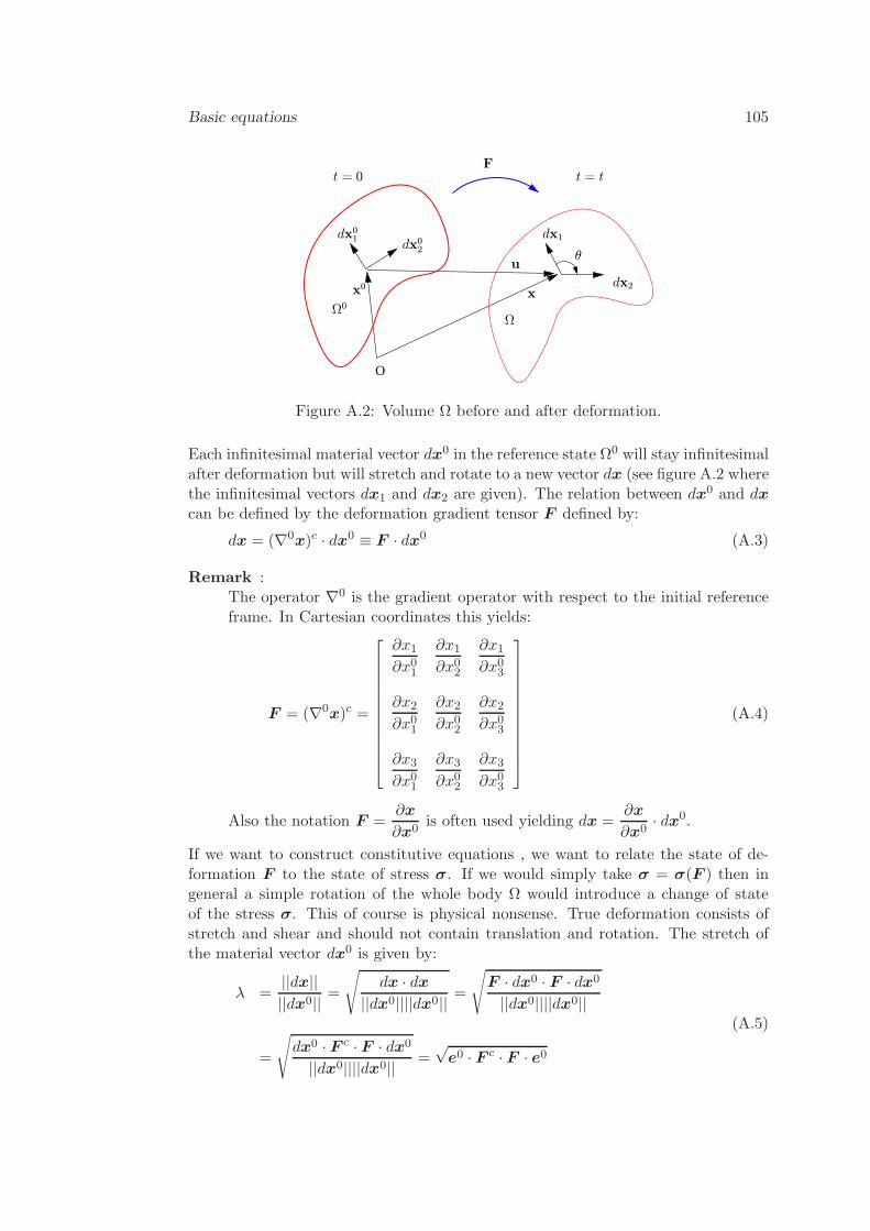
Basic equations 105
t = 0
Ω0
dx01
x0
dx02
F
Ω
u
x
dx1
θ
t = t
dx2
O
Figure A.2: Volume Ω before and after deformation.
Each infinitesimal material vector dx0 in the reference state Ω0 will stay infinitesimalafter deformation but will stretch and rotate to a new vector dx (see figure A.2 wherethe infinitesimal vectors dx1 and dx2 are given). The relation between dx0 and dxcan be defined by the deformation gradient tensor F defined by:
dx = (∇0x)c · dx0 ≡ F · dx0 (A.3)
Remark :The operator ∇0 is the gradient operator with respect to the initial referenceframe. In Cartesian coordinates this yields:
F = (∇0x)c =
∂x1∂x01
∂x1∂x02
∂x1∂x03
∂x2∂x01
∂x2∂x02
∂x2∂x03
∂x3∂x01
∂x3∂x02
∂x3∂x03
(A.4)
Also the notation F =∂x
∂x0is often used yielding dx =
∂x
∂x0· dx0.
If we want to construct constitutive equations , we want to relate the state of de-formation F to the state of stress σ. If we would simply take σ = σ(F ) then ingeneral a simple rotation of the whole body Ω would introduce a change of stateof the stress σ. This of course is physical nonsense. True deformation consists ofstretch and shear and should not contain translation and rotation. The stretch ofthe material vector dx0 is given by:
λ =||dx||||dx0|| =
√
dx · dx||dx0||||dx0|| =
√
F · dx0 · F · dx0
||dx0||||dx0||
=
√
dx0 · F c · F · dx0
||dx0||||dx0|| =√e0 · F c · F · e0
(A.5)
106 Cardiovascular Fluid Mechanics - lecture notes
with e0 = dx0/||dx0|| the unit vector in the direction of dx0 and F c the transposeof F . The shear deformation between two initially perpendicular material vectorsdx0
1 and dx02 is determined by the angle θ between the vectors after deformation
(see figure A.2):
cos(θ) =dx1 · dx2√
dx1 · dx1
√dx2 · dx2
=e01 · F c · F · e02
√
e01 · F c · F · e01√
e02 · F c · F · e02
(A.6)
Equations (A.5) and (A.6) show that true deformation can be described by theCauchy-Green deformation tensor C given by:
C = F c · F (A.7)
Note that in the derivation of the stretch λ and the shear θ the vectors dx, dx1 anddx2 are eliminated using the definition of the deformation gradient tensor F . Thismeans that the stretch and shear is defined with respect to the initial geometry Ω0.This is common in solid mechanics where the initial state is mostly well known andfree of stress.
In a similar way one can derive:
λ =||dx||||dx0|| =
√e · F · F c · e (A.8)
and:
cos(θ) =e1 · F · F c · e2√
e1 · F · F c · e1√e2 · F · F c · e2
(A.9)
Note that now the stretch and shear is defined with respect to the new (deformed)geometry, which is more suitable for fluids but also commonly used for rubber-likesolids.The tensor product
B = F · F c (A.10)
is called the Finger tensor.
Remark :The Finger tensor can also be derived by decomposing the deformation gradi-ent tensor into a stretching part U and a rotation R:
F = U ·R (A.11)
By multiplying F with its transpose (F ·F c = U ·R·(U ·R)c = U ·R·Rc ·U c =U ·U c), the rotation is removed since for rotation R ·Rc = I must hold.
Unlike the deformation gradient tensor F the Cauchy-Green deformation tensor C =F c ·F and the Finger tensor B = F ·F c both can be used to construct constitutiverelations relating the state of deformation with the state of stress without introducingspurious stresses after simple rotation.
Basic equations 107
A.2.3 Velocity and rate of deformation
In fluid mechanics not only the deformation but also the rate of deformation is ofimportance. The rate of deformation depends on the relative velocity dv between twopoints defined by the material vector dx. The velocity of material points x = x(x0, t)is defined by the rate of displacement:
v(x0, t) = u(x0, t)
= lim∆t→0
u(x0, t+∆t)− u(x0, t)
∆t
(A.12)
Together with the definition of the displacement (A.2) this yields:
v(x0, t) = lim∆t→0
x(x0, t+∆t)− x(x0, t)
∆t
= x(x0, t)
(A.13)
The rate of change of a infinitesimal material vector dx follows from (A.3) and reads:
dv = dx = F · dx0 (A.14)
The infinitesimal velocity can also be related to the infinitesimal material vectoraccording to:
dv =∂v
∂x· dx+
∂v
∂tdt (A.15)
and for a fixed instant of time (dt = 0):
dv =∂v
∂x· dx ≡ L · dx (A.16)
L is called the velocity gradient tensor.Using (A.16) this yields L · dx = dv = dx = F · dx0 = F · F−1dx, showing thatthe tensor F is defined by the tensor product of the velocity gradient tensor and thedeformation gradient tensor:
F = L · F (A.17)
The velocity gradient tensor L is often written as the dyadic product of the gradientvector ∇ and the velocity vector v:
L =∂v
∂x= (∇v)c (A.18)
If we want to relate the rate of deformation to the state of stress we must decomposeL into a part that describes the rate of deformation and a part that represents therate of rotation. This is achieved by the following decomposition:
L = D +Ω (A.19)
with:
D = U = 12 (L+Lc) = 1
2(∇v + (∇v)c) (A.20)
108 Cardiovascular Fluid Mechanics - lecture notes
Ω = R = 12(L−Lc) = 1
2(∇v − (∇v)c) (A.21)
2D (also written as γ) is the rate of deformation or rate of strain tensor and Ω
is the vorticity or spin tensor. This can be derived readily if we realize that in(A.14) we are only interested in the instantaneous rate of separation of points, i.e.we consider a deformation that takes place in an infinitesimal period of time dt sox0 → x. In that case we have after combination of (A.11) and (A.17):
limx0→x
L · F = limx0→x
(U ·R+U · R) (A.22)
Since L, U and R are defined in the current reference state they only depend on x
and t and do not depend on x0 we get:
L · limx0→x
F = U · limx0→x
R+ limx0→x
U · R (A.23)
and thus by virtue of limx0→x
F = limx0→x
U = limx0→x
R = I:
L = U + R (A.24)
So, the velocity gradient tensor L is the sum of the rate of stretching tensor U andthe rate of rotation tensor R.
A.2.4 Constitutive equations
For later use in deriving constitutive equations the following relations are given:
B = F · F c + F · F c
= L · F · F c + F · F c ·Lc
= L ·B +B ·Lc(A.25)
from which it follows that
B = 2D (A.26)
Constitutive equations for solids are oftenly constructed using a relation between thestress tensor σ and the Finger tensor B: σ = σ(B). Fluids are mostly described bya relation between the stress tensor σ and the time derivative of the Finger tensorB or by virtue of (A.26): σ = σ(D). Incompressible media (fluid or solid) on whichto a constant pressure force is exerted will not deform. Still the state of stress willchange whenever the external pressure changes. This property can incorporated inthe constitutive equations by taking:
σ = −pI + τ (B) and σ = −pI + τ (D) resp. (A.27)
The tensor τ is called the extra stress tensor.The most simple versions are found for incompressible linear elastic solids that can bedescribed σ = −pI+GB and incompressible Newtonian fluids where σ = −pI+2ηDwith p the pressure, G the shear modulus and η the dynamic viscosity.Viscoelastic materials (fluids or solids) in general are characterized by a constitutiveequation of the form: τ = τ (B, B, B, ...). In the sections that follow these relationsbetween stress and strain will be used in different forms.
Basic equations 109
A.3 Equations of motion
The equations needed for the determination of the variables pressure (p) and velocity(v) can be derived by requiring conservation of mass, momentum and energy offluid moving through a small control volume Ω. A general procedure to obtain theseequations is provided by the transport theorem of Reynolds.
A.3.1 Reynolds’ transport theorem
Consider an arbitrary volume Ω = Ω(t) with boundary surface Γ = Γ(t) not neces-sarily moving with the fluid and let Ψ(x, t) be a scalar, vector or tensor function ofspace and time defined in Ω(t). The volume integral:
∫
Ω(t)
Ψ(x, t)dΩ (A.28)
is a well defined function of time only. The rate of change of Ψ in Ω(t) is given by:
d
dt
∫
Ω(t)
Ψ(x, t)dΩ =
lim∆t→0
1
∆t
∫
Ω(t+∆t)
Ψ(x, t+∆t)dΩ−∫
Ω(t)
Ψ(x, t)dΩ
.
(A.29)
If the boundary Γ(t) moves with velocity vΓ this will introduce a flux of Ψ propor-tional to vΓ · n. As a consequence:
∫
Ω(t+∆t)
Ψ(x, t+∆t)dΩ =
∫
Ω(t)
Ψ(x, t+∆t)dΩ+∆t
∫
Γ(t)
Ψ(x, t+∆t)vΓ ·ndΓ(A.30)
The rate of change of Ψ then can be written as:
d
dt
∫
Ω(t)
ΨdΩ = lim∆t→0
1
∆t
∫
Ω(t)
Ψ(x, t+∆t)dΩ +
∆t
∫
Γ(t)
Ψ(x, t+∆t)vΓ · ndΓ−∫
Ω(t)
Ψ(x, t)dΩ
=
∫
Ω(t)
lim∆t→0
1
∆t[Ψ(x, t+∆t)dΩ−Ψ(x, t)dΩ]+
∫
Γ(t)
lim∆t→0
Ψ(x, t+∆t)vΓ · ndΓ
(A.31)
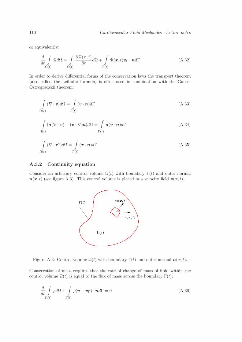
110 Cardiovascular Fluid Mechanics - lecture notes
or equivalently:
d
dt
∫
Ω(t)
ΨdΩ =
∫
Ω(t)
∂Ψ(x, t)
∂tdΩ+
∫
Γ(t)
Ψ(x, t)vΓ · ndΓ (A.32)
In order to derive differential forms of the conservation laws the transport theorem(also called the Leibnitz formula) is often used in combination with the Gauss-Ostrogradskii theorem:
∫
Ω(t)
(∇ · v)dΩ =
∫
Γ(t)
(v · n)dΓ (A.33)
∫
Ω(t)
(a(∇ · v) + (v · ∇)a)dΩ =
∫
Γ(t)
a(v · n)dΓ (A.34)
∫
Ω(t)
(∇ · τ c)dΩ =
∫
Γ(t)
(τ · n)dΓ (A.35)
A.3.2 Continuity equation
Consider an arbitrary control volume Ω(t) with boundary Γ(t) and outer normaln(x, t) (see figure A.3). This control volume is placed in a velocity field v(x, t).(t) (t) n(x; t)v(x; t)Figure A.3: Control volume Ω(t) with boundary Γ(t) and outer normal n(x, t).
Conservation of mass requires that the rate of change of mass of fluid within thecontrol volume Ω(t) is equal to the flux of mass across the boundary Γ(t):
d
dt
∫
Ω(t)
ρdΩ+
∫
Γ(t)
ρ(v − vΓ) · ndΓ = 0 (A.36)
Basic equations 111
The first term can be rewritten with Leibnitz formula. Applying the Gauss-Ostrogradskiidivergence theorem this yields:
∫
Ω(t)
[
∂ρ
∂t+∇ · (ρv)
]
dΩ = 0 (A.37)
Since this equation must hold for all arbitrary control volumes Ω(t), the followingdifferential form can be derived:
∂ρ
∂t+∇ · (ρv) = 0 (A.38)
This differential form of the equation for conservation of mass is called the continuityequation.
A.3.3 The momentum equation
Consider again the control volume Ω(t) with boundary Γ(t) and outer normal n(x, t)placed in a velocity field v(x, t). The rate of change of linear momentum summedwith the flux of momentum through the boundary Γ(t) is equal to the sum of theexternal volume and boundary forces.
d
dt
∫
Ω(t)
ρvdΩ+
∫
Γ(t)
ρv(v − vΓ) · ndΓ =
∫
Ω(t)
ρfdΩ+
∫
Γ(t)
sdΓ (A.39)
Here f denotes the body force per unit of mass and s denotes the stress vector actingon the boundary Γ of Ω. If again the control volume is considered to be fixed inspace one can apply the Gauss-Ostrogradskii divergence theorem. Then, making useof the Cauchy stress tensor σ defined by (see (A.1):
s = n · σ (A.40)
equation (A.39) yields:
∫
Ω(t)
[
∂ρv
∂t+ ρv(∇ · v) + (v · ∇)ρv
]
dΩ =
∫
Ω(t)
[ρf +∇ · σ] dΩ (A.41)
After substitution of the continuity equation (A.38) the differential form of (A.41)will be the momentum equation:
ρ∂v
∂t+ ρ(v · ∇)v = ρf +∇ · σ (A.42)
112 Cardiovascular Fluid Mechanics - lecture notes
A.3.4 Initial and boundary conditions
Without going into the mathematics needed to prove that a unique solution of theequations of motion (A.38) and (A.42) exists, the boundary conditions that areneeded to solve these equations can be deduced from the integral formulation ofthe continuity and momentum equations (A.36) and (A.39) respectively. From themomentum equation (A.39) it can be seen that both the velocity and the stressvector could be prescribed on the boundary. Since these quantities are related byvirtue of a constitutive equation, only one of them (for each coordinate direction)should be used. So for each local boundary coordinate direction one can describeeither its velocity v or its stress vector s. Defining n as the outer normal and ti(i = 1, 2) the tangential unit vectors to the boundary Γ this yields:
in normal direction:the Dirichlet condition:
(v · n) = vnΓ
or Neumann condition:(σ · n) · n = (s · n)
in tangential directions:the Dirichlet conditions:
(v · ti) = vtiΓ i = 1, 2
or Neumann conditions:(σ · n) · ti = (s · ti)
(A.43)
For time-dependent problems initial conditions for velocity and stress must be givenas well.
A.4 Incompressible viscous flow
For incompressible isothermal flow the density ρ is constant in space and time andthe mass conservation or continuity equation is given by:
∇ · v = 0 (A.44)
In a viscous fluid, besides pressure forces also viscous forces contribute to the stresstensor and in general the total stress tensor can be written as (see appendix A):
σ = −pI+ τ (B). (A.45)
In order to find solutions of the equations of motion the viscous stress tensor τ
has to be related to the kinematics of the flow by means of a constitutive equationdepending on the rheological properties of the fluid. In this section only Newtonianfluids will be discussed briefly.
A.4.1 Newtonian flow
In Newtonian flow there is a linear relation between the viscous stress τ and therate of deformation tensor γ according to:
τ = 2ηD = ηγ (A.46)
Basic equations 113
with η the dynamic viscosity and the rate of deformation tensor defined as:
γ = ∇v + (∇v)c. (A.47)
Substitution in the momentum equation yields the Navier-Stokes equations:
ρ∂v
∂t+ ρ(v · ∇)v = ρf −∇p+ η∇2v
∇ · v = 0
(A.48)
After introduction of the non-dimensional variables: x∗ = x/L, v∗ = v/V , t∗ = t/θ,p∗ = p/ρV 2 and f∗ = f/g, the dimensionless Navier-Stokes equations for incom-pressible Newtonian flow become (after dropping the superscript ∗):
Sr∂v
∂t+ (v · ∇)v =
1
Fr2f −∇p+ 1
Re∇2v
∇ · v = 0
(A.49)
With the dimensionless parameters:
Sr =L
θVStrouhal number
Re =ρV L
ηReynolds number
Fr =V√gL
Froude number
(A.50)
A.5 Incompressible in-viscid flow
For incompressible isothermal flow the density ρ is constant in space and time andthe mass conservation or continuity equation is given by:
∇ · v = 0 (A.51)
In an in-viscid fluid, the only surface force is due to the pressure, which acts normalto the surface. In that case the stress tensor can be written as:
σ = −pI (A.52)
The momentum and continuity equations then lead to the Euler equations:
ρ∂v
∂t+ ρ(v · ∇)v = ρf −∇p
∇ · v = 0
(A.53)
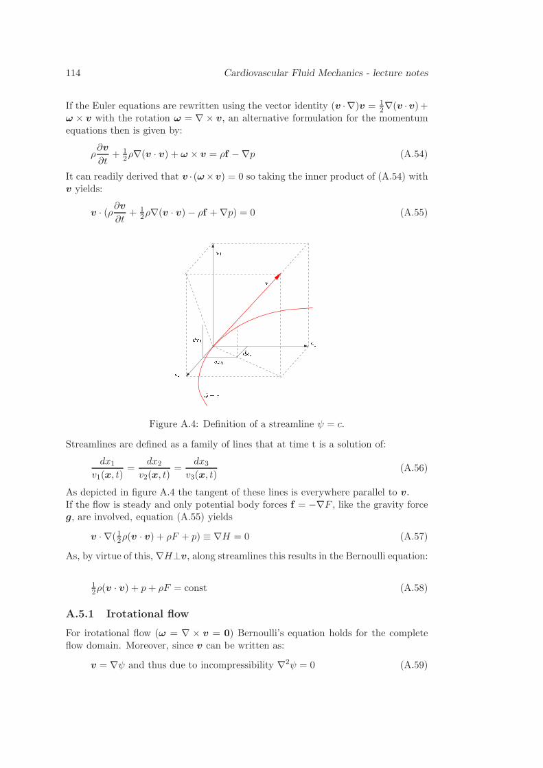
114 Cardiovascular Fluid Mechanics - lecture notes
If the Euler equations are rewritten using the vector identity (v ·∇)v = 12∇(v ·v)+
ω × v with the rotation ω = ∇ × v, an alternative formulation for the momentumequations then is given by:
ρ∂v
∂t+ 1
2ρ∇(v · v) + ω × v = ρf −∇p (A.54)
It can readily derived that v · (ω×v) = 0 so taking the inner product of (A.54) withv yields:
v · (ρ∂v∂t
+ 12ρ∇(v · v)− ρf +∇p) = 0 (A.55)
v3
dx2dx3v2 dx1 v1
= c
v
Figure A.4: Definition of a streamline ψ = c.
Streamlines are defined as a family of lines that at time t is a solution of:
dx1v1(x, t)
=dx2
v2(x, t)=
dx3v3(x, t)
(A.56)
As depicted in figure A.4 the tangent of these lines is everywhere parallel to v.If the flow is steady and only potential body forces f = −∇F , like the gravity forceg, are involved, equation (A.55) yields
v · ∇(12ρ(v · v) + ρF + p) ≡ ∇H = 0 (A.57)
As, by virtue of this, ∇H⊥v, along streamlines this results in the Bernoulli equation:
12ρ(v · v) + p+ ρF = const (A.58)
A.5.1 Irotational flow
For irotational flow (ω = ∇ × v = 0) Bernoulli’s equation holds for the completeflow domain. Moreover, since v can be written as:
v = ∇ψ and thus due to incompressibility ∇2ψ = 0 (A.59)
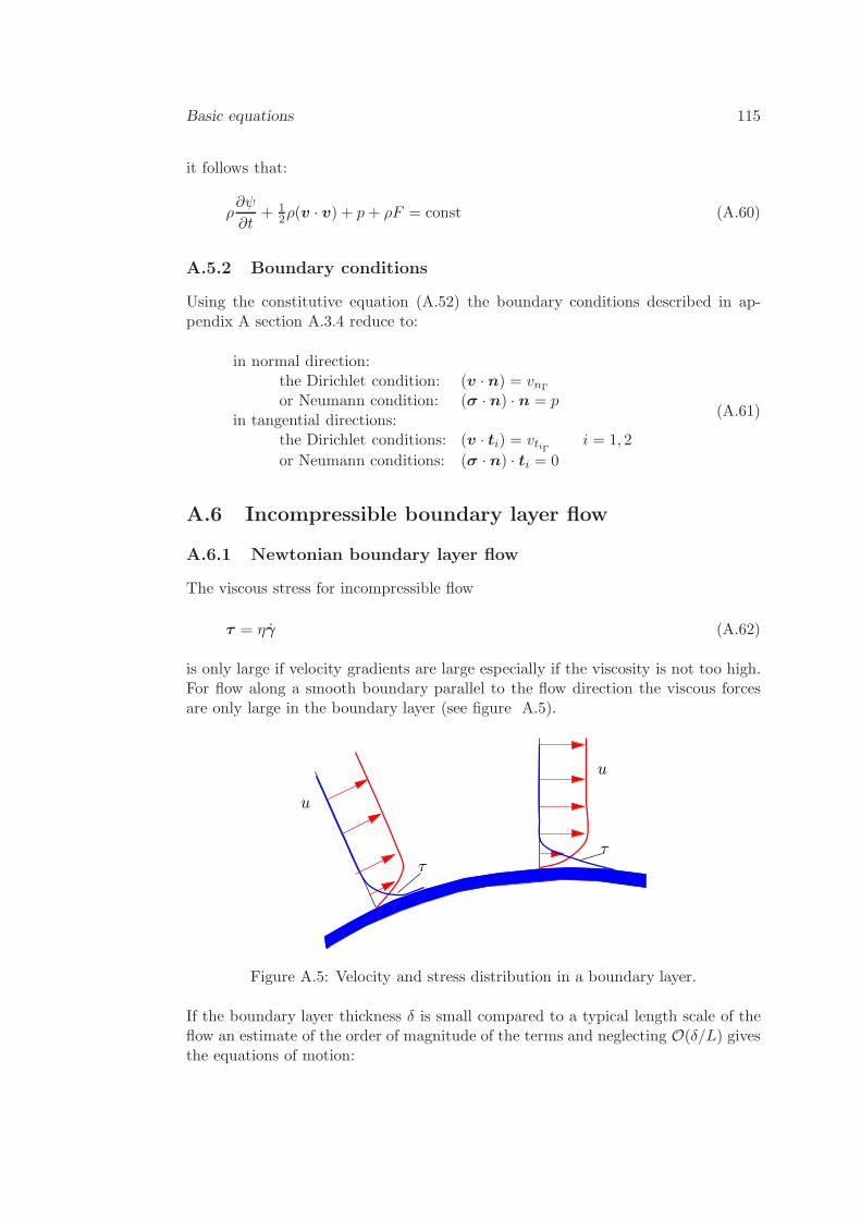
Basic equations 115
it follows that:
ρ∂ψ
∂t+ 1
2ρ(v · v) + p+ ρF = const (A.60)
A.5.2 Boundary conditions
Using the constitutive equation (A.52) the boundary conditions described in ap-pendix A section A.3.4 reduce to:
in normal direction:the Dirichlet condition: (v · n) = vnΓ
or Neumann condition: (σ · n) · n = pin tangential directions:
the Dirichlet conditions: (v · ti) = vtiΓ i = 1, 2
or Neumann conditions: (σ · n) · ti = 0
(A.61)
A.6 Incompressible boundary layer flow
A.6.1 Newtonian boundary layer flow
The viscous stress for incompressible flow
τ = ηγ (A.62)
is only large if velocity gradients are large especially if the viscosity is not too high.For flow along a smooth boundary parallel to the flow direction the viscous forcesare only large in the boundary layer (see figure A.5).
u
u
τ
τ
Figure A.5: Velocity and stress distribution in a boundary layer.
If the boundary layer thickness δ is small compared to a typical length scale of theflow an estimate of the order of magnitude of the terms and neglecting O(δ/L) givesthe equations of motion:
116 Cardiovascular Fluid Mechanics - lecture notes
∂v1∂x1
+∂v2∂x2
= 0
ρ∂v1∂t
+ ρv1∂v1∂x1
+ ρv2∂v1∂x2
= − ∂p
∂x1+ η
∂2v1∂x22
∂p
∂x2= 0
(A.63)
Outside the boundary layer the flow is assumed to be in-viscid and application ofBernoulli in combination with the second equation of (A.63) gives:
− ∂p
∂x1= ρV
∂V
∂x1(A.64)
A.6.2 Initial and boundary conditions
This set of equations requires initial conditions:
v1(x10 , x2, 0) = v01(x1, x2) (A.65)
and boundary conditions:
v1(x10 , x2, t) = v10(x2, t)v1(x1, 0, t) = 0v1(x1, δ, t) = V (x1, t)
(A.66)
The boundary layer thickness δ can often be estimated by stating that at x2 = δ theviscous forces O(ηV/ρδ2) are of the same magnitude as the stationary inertia forcesO(V 2/L) or in-stationary inertia forces O(V/θ).
Bibliography
Abramowitz, M. and Stegun, I. (1964). Handbook of Mathematical functions. DoverPublications, Dover.
Batchelor, G. (1967). An Introduction to Fluid Mechanics. Cambridge UniversityPress, Cambridge.
Batchelor, G. K. (1977). The effect of brownian motion on the bulk stress in asuspension of spherical particles. J. Fluid Mech., 83, 97–117.
Bingham, E. (1922). Fluidity and Plasticity . McGraw-Hill, New York.
Bird, R., Stewart, W., and Lightfood, E. (1960). Transport phenomena. John Wiley& Sons, New York.
Bird, R., Armstrong, R., and Hassager, O. (1987). Dynamics of Polymer Liquids.John Wiley & Sons, New York.
Chadwick, P. (1976). Continuum Mechanics. John Wiley & Sons, New York.
Chien, S., Usami, S., Dellenback, R. J., and Gregersen, M. I. (1969). Shear-dependent deformation of erythrocyts in rheology of human blood. American
Journal of Physiology , 219, 136–142.
Collins, W. M. and Dennis, S. C. R. (1975). The steady motion of a viscous fluid ina curved tube. Q.J.Mech. Appl. Math, 28, 133–156.
Fung, Y. (1993a). Mechanical Properties and Active Remodeling of Blood Vessels,chapter 8, pages 321–391. In Fung (1993b), 2nd edition.
Fung, Y., Fronek, K., and Patitucci, P. (1979). Pseudoelasticity of arteries and thechoice of its mathematical ex pression. American Journal of Physiology , 237,H620–H631.
Fung, Y. C. (1993b). Biomechanics, Mechanical Properties of Living Tissues.Springer Verlag, New York Berlin Heidelberg, 2nd edition.
Guyton, A. C. (1967). Textbook of Medical Physiology . Saunders.
Kasyanov, V. and Knet-s, I. (1974). Deformation energy function of large humanblood vessels. Mekhanika Polimerov , 1, 122–128.
117
118 Cardiovascular Fluid Mechanics - lecture notes
Macosko, C. W. (1994). Rheology, principles, measurements and applications. VCHpublishers, Inc., New York.
McMillan, D., Strigberger, J., and Utterback, N. (1987). Rapidly recovered transientflow resistance: a newly discovered property of blood. Am. J. Physiol., 253, 919–926.
Milnor, W. R. (1989). Hemodynamics. Williams & Wilkins, Baltimore, Hong Kong,London, Sidney.
Pedley, T. (1980). The fluid mechanics of large blood vessels. Cambridge UniversityPress, Cambridge.
Quemada, D. (1978). Rheology of concentrated disperse systems. ii. a model fornon-newtonian shear viscosity in steady flows. Rheol. Acta, 17, 632–642.
Rhodin, J. A. G. (1980). Architecture of the Vessel Wall , chapter 1, pages 1–31.
Rosenblatt, J. S. (1988). The rheology of blood: a structured fluid approach based on
rouleau behaviour . Ph.D. thesis, University of California, Berkeley.
Schlichting, H. (1960). Boundary Layer Theory . McGraw-Hill, New York.
Schmid-Schonbein, H., Wells, R., and J.Goldstone (1971). Fluid drop-like behaviorof erythrocytes- disturbance in pathology and its quantification. Biorheology , 7,227–234.
Thurston, G. (1973). Frequency and shear rate dependence of viscoelasticity ofhuman blood. Biorheology , 10, 375–381.
Ward-Smith, A. (1980). Internal fluid flow . Oxford.
Womersley, J. R. (1957). The mathematical analysis of the arterial circulation in astate of oscillatory motion. Technical report wadc-tr-56-614, Wright Air Develop-ment Center.
Index
admittance, 71–73effective, 78
aggregation, 103albumin, 84arterial system, 4, 5
dimensions, 4arteries
aorta, 3pulmonary, 2
arteriolespulmonary, 2
atriumleft, 2right, 2
Bernoulli equation, 30Bessel functions, 35blood
generalized Newtonian models, 90Newtonian models, 89plasma, 84rheology, 86, 102viscoelastic models, 94viscosity, 88
Bolzmann’s superposition principle, 94boundary layer
thickness, 40boundary layer flow, 30branched tube
flow, 49
capillary system, 5dimensions, 4
cardiac work, 81cardiovascular system, 2Careau-Yasuda model, 91Casson model, 91Cauchy stress tensor, 16Cauchy-Green deformation tensor, 18
circulation
pulmonary, 2
systemic, 2, 4
coagulation, 102
collagen, 53
compliance, 7, 11, 60, 69
compression modulus, 57
constitutive equations, 20
continuity equation, 22
contraction
atrial, 3
ventricular, 3
curved tube
steady entrance flow, 41
steady fully developed flow, 45
unsteady fully developed flow, 47
Dean number, 46
Deborah number, 96
deformation
Cauchy-Green deformation tensor, 18
deformation gradient tensor, 16, 17
Finger tensor, 18
linear elastic, 56
neo-Hookean, 56
rate of deformation tensor, 19, 20
shear, 18
stretch, 17
diastole, 3
Dirichlet conditions, 24
discrete transitions, 75
displacement
displacement vector, 16
distensibility, 7, 61, 69
distensible tube
fluid flow, 65
distensible tubes
wave propagation, 67
119
120 Cardiovascular Fluid Mechanics - lecture notes
effective viscosity, 109, 113elastic solids, 20elastin, 53endothelial cells, 5, 53entrance flow
curved tube, 41rigid tube, 39
entrance lengthoscillating flow, 41steady flow, 40
equations of motion, 21erythrocytes, 84Euler equations, 29extra stress tensor, 20
fibrinogen, 84Finger tensor, 18
flowaortic, 3arterioles and venules, 112branched tubes, 49capillaries, 114
curved tube, 41entrance, 39Fourier decomposition, 8, 10incompresible in-viscid, 29incompressible boundary layer flow,
30incompressible viscous, 28
irotational, 30Newtonian, 28secondary flow in curved tube, 43small arteries and veins, 108
Froude number, 28
fully developed flowcurved tube, 45straight tube, 32
Gauss-Ostrogradskii theorem, 22globulins, 84
heart, 2
minute volume, 5
impedance, 71input, 12longitudinal, 12, 38
transverse, 12initial and boundary conditions, 24
Leibnitz formula, 22leucocytes, 86
micro circulation, 5micro-circulation, 107Moens Korteweg wave speed, 71momentum equation, 23
Navier-Stokes equations, 28cylindrical coordinates, 32dimensionless, 28toroidal coordinates, 45
Neumann conditions, 24Newtonian flow, 28
fully developed, 32Newtonian fluids, 20
peripheral resitance, 11plasma, 84
density, 84viscosity, 84, 103
platelets, 86Poisson ratio, 58power-law model, 91pressure
aortic, 3Fourier decomposition, 8, 10pulmonary, 3systemic, 3transmural, 6ventricular, 3
Quemada model, 102
rate of deformation tensor, 20, 28red blood cells
aggregation, 103concentration, 110, 113deforrmation, 103viscosity, 84
reflectionmultiple, 78
reflection coefficient, 76resistance
periferal, 5
Bibliography 121
Reynolds number, 28Reynolds’ transport theorem, 21rheology, 86rheology of blood, 102rheometry, 87Rosenblatt model, 105rotation tensor, 18
secondary flow, 43secondary boundary layer, 47
shear, 18shear modulus, 20, 56smooth muscle cells, 54spin tensor, 20straight tube
entrance flow, 39fully developed flow, 32longitudinal impedance, 38oscillating entrance flow, 41steady entrance flow, 40velocity profiles, 33wall shear stress, 36
streamlines, 29stress
state of, 16stress tensor, 16stress vector, 16
stretch, 17stretching tensor, 18Strouhal number, 28suspensions, 100
Quemada model, 102rheology, 100
systole, 3
transmission coefficient, 76
valveaortic, 3mitral, 3
vasoconstriction, 5vasodilattion, 5veins
venae cavae, 2velocity
velocity gradient tensor, 19velocity vector, 19
velocity profilesarbitrary Womersley number, 34
large Womersley number, 34
rigid tube, 33
small Womersley number, 33
venoconstriction, 5venous system, 5
dimensions, 4
ventricle
left, 2
right, 2vessel wall
adventitia, 53
effective Young’s modulus, 55
elastic behavior, 54
incremental Young’s modulus, 55intima, 52, 53
media, 53
morphology, 52
smooth muscle cells, 53
viscoelastic behavior, 55Young’s modulus, 55
viscoelastic fluids, 20
viscoelastic solids, 20
viscosity
dynamic, 20
effective viscosity, 109, 113vorticity tensor, 20
wall shear stress
rigid tubes, 36
wave attenuation, 70
wave number, 70wave reflection, 75
wave speed, 65, 70
Moens Korteweg, 71
waves
angular frequency, 64attenuation constant, 70
complex amplitude, 64, 70
complex notation, 64
flow, 6
phase velocity, 70pressure, 6
wave attenuation, 70
wave length, 64
122 Cardiovascular Fluid Mechanics - lecture notes
wave number, 64, 70wave speed, 70
Weissenberg number, 96windkessel model, 11, 64
impedance, 64Womersley function
approximation, 37definition, 36
Womersley numberdefinition, 32values in arteries, 33
Womersley profiles, 35, 67
Young’s modulus, 58complex modulus, 70