Cardiff Economics

Working Papers

Emma M. Iglesias and Garry D.A. Phillips

Almost Unbiased Estimation in Simultaneous Equations

Models with Strong and / or Weak Instruments

E2011/19

CARDIFF BUSINESS SCHOOL

WORKING PAPER SERIES

This working paper is produced for discussion purpose only. These working papers are expected to be published in

due course, in revised form, and should not be quoted or cited without the author’s written permission.

Cardiff Economics Working Papers are available online from: http://www.cardiff.ac.uk/carbs/econ/workingpapers

Enquiries: EconWP@cardiff.ac.uk

ISSN 1749-6101

August 2011

Cardiff Business School

Cardiff University

Colum Drive

Cardiff CF10 3EU

United Kingdom

t: +44 (0)29 2087 4000

f: +44 (0)29 2087 4419

www.cardiff.ac.uk/carbs

Almost Unbiased Estimation in Simultaneous Equations

Models with Strong and / or Weak Instruments�

Emma M. Iglesias

University of A Coruña

and Garry D.A. Phillips

Cardi¤ University

This version: August 2011

Abstract

We propose two simple bias reduction procedures that apply to estimators in a general static

simultaneous equation model and which are valid under reatively weak distributional assump-

tions for the erros.. Standard jackknife estimators, as applied to 2SLS, may not reduce the bias

of the exogenous variable coe¢ cient estimators since the estimator biases are not monotonically

non-increasing with sample size (a necessary condition for successful bias reduction) and they

have moments only up to the order of overidenti�cation. Our proposed approaches do not have

either of these drawbacks. (1) In the �rst procedure, both endogenous and exogenous variable

parameter estimators are unbiased to order T�2 and when implemented for k�class estimatorsfor which k < 1, the higher order moments will exist. (2) An alternative second approach is

based on taking linear combinations of k�class estimators for k < 1. In general, this yields

estimators which are unbiased to order T�1 and which possess higher moments. We also prove

theoretically how the combined k�class estimator produces a smaller mean squared error than2SLS when the degree of overidenti�cation of the system is larger than 8. Moreover, the com-

bined k�class estimators remain unbiased to order T�1 even if there are redundant variables(including weak instruments) in any part of the simultaneous equation system, and we can allow

for any number of endogenous variables. The performance of the two procedures is compared

�We are grateful for very helpful comments from Bruce Hansen, Grant Hillier, Gary Solon, Tim Vogelsang and

seminar participants at Harvard / MIT, Michigan State University, Purdue University, Singapore Management Uni-

versity, Tilburg University and at University of Montreal; and also from participants at the 2006 Far Eastern Meeting

of the Econometric Society, the 2006 Midwest Econometrics Group and the 2006 and 2008 European Meetings of

the Econometric Society. We owe special debt to Je¤ Wooldridge for many comments and suggestions that we have

obtained both in the theoretical and in the application section. Financial support from the MSU Intramural Research

Grants Program is gratefully acknowledged.

1

with 2SLS in a number of Monte Carlo experiments using a simple two equation model. Fi-

nally, an application shows the usefulness of our new estimator in practice versus competitor

estimators.

Keywords: Combined k�class estimators; Bias correction; Weak instruments; Endogenousand exogenous parameter estimators; Permanent Income Hypothesis.

JEL classi�cation: C12; C13; C30; C51, D12, D31, D91, E21, E40.

1 Introduction

Instrumental variable (IV ) estimators (see e.g. Hausman (1983), Staiger and Stock (1997), and

Hahn and Hausman (2002a, 2002b, 2003)) are known to have very poor �nite sample properties,

both when the size of the sample is very small, and / or when the instruments are weak (see eg.

Nelson and Startz (1990a, 1990b) and Staiger and Stock (1997)). Andrews and Stock (2006) recently

provided an extensive and updated review of the literature of simultaneous equations systems and

weak instruments.

If the problem is that we simply have a small sample then traditional higher order �strong IV

asymptotics�may provide an appropriate means of analysis; however, this is not enough in the weak

instruments context. Therefore, in the weak instruments literature, in order to analyze the perfor-

mance of instrumental variable estimators, several di¤erent types of asymptotics have been proposed:

for example, �weak IV asymptotics�, �many IV asymptotics�and �many weak IV asymptotics�,

see Andrews and Stock (2006).

In relation to bias, Richardson and Wu (1971) found the exact bias of the Two Stage Least

Squares (2SLS) estimator assuming normal errors while Sawa (1972) gave the exact bias for the

general k�class estimator. More recently, Chao and Swanson (2007) have shown the asymptotic biasof the 2SLS estimator using the �weak IV asymptotics�of Staiger and Stock (1997), allowing for

possibly non-normal errors and stochastic instruments. All these results were derived in the context

of an equation containing two endogenous variables. The exact density for instrumental variable

estimators in the general case is given in Phillips (1980). However, the resulting moment expressions

are complex and we shall not consider them here.

In this paper we are interested in constructing two very simple bias correction procedures that

can work in a range of cases, including when we have weak instruments. Recently Davidson and

Mackinnon (2006), in a comprehensive Monte Carlo study of a two endogenous variable equation,

found little evidence of support for the use of the Jackknife IV estimator introduced by Phillips and

Hale (1977), and later used by Angrist, Imbens and Krueger (1999) and Blomquist and Dahlberg

(1999), especially in the presence of weak instruments. In addition, they concluded that there is no

2

clear advantage in using Limited Information Maximum Likelihood (LIML) over 2SLS in practice,

particularly in the context of weak instruments, while estimators which possess moments tend to

perform better than those which do not. So there remain questions about the �nite sample properties

of the standard simultaneous equation estimators especially in the weak instrument context.

For our analysis, we deal with a broad setting where we allow for a general number of endogenous

and exogenous variables in the system. We �rst develop a bias reduction approach that will apply

to both endogenous and exogenous variable parameter estimators. We use both large�T asymp-

totic analysis and exact �nite sample results, to propose a procedure to reduce the bias of k�classestimators that works particularly well when the system includes weak instruments since, in this

case, any e¢ ciency loss is minimized; however, we do not assume that all instruments are weak. We

examine the bias of 2SLS and also other k�class estimators, and we show that the bias to orderT�2 is eliminated when the number of exogenous variables excluded from the equation of interest is

chosen so that the parameters are �notionally�overidenti�ed of order one. This is achieved through

the introduction of redundant regressors. While the resulting bias corrected estimators are more

dispersed, the increased dispersion will be less the weaker the instruments we have available in the

system for use as redundant regressors; hence, the availability of weak instruments is actually a

blessing in context. We show in our simulations for sample sizes T = 100, that the bias correction is

so impressive, that there are some indications that the bias may be of even smaller order.

The above procedure, as applied to 2SLS, has the main disadvantage that whereas the estimator

has a �nite bias, the variance does not exist. We therefore consider other k�class estimators where wecan continue to get a reduction of the bias by using our approach, and where higher order moments

will exist. In particular, we consider the estimators where k = 1�T�3 and k = 1�T�1. The former isespecially interesting since its behavior is very close to that of 2SLS yet higher moments are de�ned.

Note that LIML is known to be median unbiased up order T�1 (see Rothenberg (1983)), while with

our bias correction mechanism we can get estimators that are unbiased to order T�2.

A second procedure that we analyze is based on a linear combination of k�class estimators withk <1 that is unbiased to order T�1; has higher moments, and generally improves on Mean Squared

Error (MSE) compared to 2SLS when there are a moderate or larger number of (weak or strong)

instruments in the system. Hence whereas the �rst of our bias correction procedures is likely to be

attractive mainly when there are weak instruments in the system, the second procedure does not

depend on this.

The bias correction procedures proposed in this paper have the particular advantage over other

bias reduction techniques e.g, Fuller�s corrected LIML estimator, of not depending on assuming

normality for the errors. Indeed they are valid under relatively weak assumptions and in the case

of the second procedure the errors need not even be independently distributed.. In addition they

3

may have several other advantages.. First, the standard delete one jackknife estimator referred to

as JN2SLS recently proposed by Hahn, Hausman and Kuersteiner (2004) does generally reduce the

bias of the endogenous variable coe¢ cient estimator but it does not necessarily reduce the bias of

non-redundant exogenous variable coe¢ cient estimators since, as Ip and Phillips (1998) show, the

exogenous coe¢ cient bias is not monotonically decreasing with the sample size. Our bias corrections

will work for both endogenous and exogenous coe¢ cient estimators.

Second, the Chao and Swanson (2007) bias correction does not work well for orders of overiden-

ti�cation smaller than 8 whereas our procedures will successfully reduce bias in such cases. Hansen,

Hausman and Newey (2008) point out that in checking �ve years of the microeconometric papers

published in the Journal of Political Economy, in the Quarterly Journal of Economics and in the

American Economic Review, 50 percent had at least 1 overidentifying restriction, 25 percent had at

least 3 and 10 per cent had 7 or more. This justi�es the need to have procedures available that can

work well in practice, at di¤erent orders of overidenti�cation and with a range of instruments. When

there is only one overidentifying restriction, the frequently used 2SLS does not have a �nite variance

and this applies in 50% of the papers analyzed above. However, our procedures based on k�classestimators for which k < 1 lead to estimators that have higher order moments and so will dominate

2SLS in this crucial case. Indeed, we show in our simulations that both our procedures work well

not only for the case of one overidentifying restriction but, more generally, for both small and large

numbers of instruments.

Third, following Hansen, Hausman and Newey (2008), we have checked the microeconometric

papers published in 2004 and 2005 for the same journals and we found that 40 per cent of them used

more than 1 included endogenous variable in their simultaneous equation models. Moreover, 2SLS

is the most commonly chosen estimation procedure. This supports the need to develop attractive

estimation methods that can deal with more than 1 included endogenous variable in the system.

Note that, in the actual econometrics literature, some of the procedures that have been developed

only allow for 1 included endogenous regressor variable (see e.g. Donald and Newey (2001)) and

they have used 2SLS as the main estimation procedure. We propose in this paper an alternative

estimation procedure that allows for any number of included endogenous variables in the equation.

Fourth, our procedures are very easy to implement and do not use a traditional �bias correction�

approach whereby the estimated bias is subtracted from the uncorrected estimate. At the same time,

the bias correction works even if we are introducing irrelevant variables in any equation of the system.

Finally, we are able to prove theoretically that both of our approaches produce unbiased estimators

up to, at least, order T�1; and also, that the approach that combines k�class estimators produces asmaller MSE than 2SLS when the equation of interest is just identi�ed, overidenti�ed of order one

and overidenti�ed at least of order 8.

4

A �nal remark is that there is a growing econometric literature concerned with nearly-weak-

identi�cation (see e.g. Caner (2007), and Antoine and Renault (2009)), where standard strong

asymptotics is valid. Our bias correction mechanisms will work for this case also.

The structure of the paper is as follows. Section 2 presents the model and it gives a summary of

large�T approximations which provide a theoretical underpinning for the bias correction. We alsodiscuss some of the exact �nite sample theory results for 2SLS which provide further theoretical

support, and we examine the weak instrument model of Staiger and Stock (1997) and Chao and

Swanson (2007). In Staiger and Stock only weak instruments are available, while in the strong

asymptotic setting, we have a mixture of weak and strong instruments. In Section 3 we discuss in

detail one possible procedure for bias correction based on introducing redundant exogenous variables

and we also consider how to choose the redundant variables by examining how the asymptotic

covariance matrix changes with the choice made. This provides criteria for selecting such variables

optimally. In Section 4 we develop a new estimator based a linear combination of k�class estimatorswith k < 1 which is unbiased to order T�1and has higher moments and we examine how to estimate

the variance of the new combined estimator. In Section 5 we present the results of simulation

experiments which indicate the usefulness of our proposed procedures. Section 6 provides an empirical

application where we show the performance of our new estimator and the results when compared

with alternative estimators such as 2SLS. Finally, Section 7 concludes. The proofs are collected in

the Appendix.

2 The simultaneous equation model

The model we shall analyze is the classical static simultaneous equation model presented in Nagar

(1959) and which appears in many textbooks. Hence we consider a simultaneous equation model

containing G equations given by

(1) Byt + �xt = ut; t = 1; 2; ::::::; T;

in which yt is a G � 1 vector of endogenous variables, xt is a R � 1 vector of strongly exogenousvariables and ut is a G� 1 vector of structural disturbances with G�G positive de�nite covariancematrix �. The matrices of structural parameters, B and � are, respectively, G�G and G�R: It isassumed that B is non-singular so that the reduced form equations corresponding to (1) are

yt = �B�1�xt +B�1ut = �xt + vt;

where � is a G � K matrix of reduced form coe¢ cients and vt is a G � 1 vector of reduced formdisturbances with a G�G positive de�nite covariance matrix :With T observations we may write

5

the system as

(2) Y B0 +X�0 = U:

Here, Y is a T � G matrix of observations on endogenous variables, X is a T � R matrix of

observations on the strongly exogenous variables and U is a T �G matrix of structural disturbances.The �rst equation of the system will be written as

(3) y1 = Y2� +X1 + u1;

where y1 and Y2 are, respectively, a T � 1 vector and a T � g1 matrix of observations on g1 + 1endogenous variables, X1 is a T � r1 matrix of observations on r1 exogenous variables, � and are,respectively, g1 � 1 and r1 � 1 vectors of unknown parameters and u1 is a T � 1 vector of normallydistributed disturbances with covariance matrix E(u1u

01) = �11IT .

We shall �nd it convenient to rewrite (3) as

(4) y1 = Y2� +X1 + u1 = Z1�+ u1;

where �0 = (�; )0 and Z1 = (Y2 : X1):

The reduced form of the system includes

Y1 = X�1 + V1;

in which Y1 = (y1 : Y2), X = (X1 : X2) is a T �R matrix of observations on R exogenous variableswith an associated R � (g1 + 1) matrix of reduced form parameters given by �1 = (�1 : �2), while

V1 = (v1 : V2) is a T � (g1 + 1) matrix of normally distributed reduced form disturbances. The

transpose of each row of V1 is independently and normally distributed with a zero mean vector and

(g1 + 1)� (g1 + 1) positive de�nite matrix 1 = (!ij). We also make the following assumption:

Assumption A. (i): The T � R matrix X is strongly exogenous and of rank K with limit

matrix limT!1 T�1X 0X = �XX ; which is R�R positive de�nite, and that (ii): Equation (3) is over-

identi�ed so that K > g1 + r1 , i.e. the number of excluded variables exceeds the number required

for the equation to be just identi�ed. In cases where second moments are analyzed we shall assume

that R exceeds g1+r1 by at least two. These over-identifying restrictions are su¢ cient to ensure that

the Nagar expansion is valid in the case considered by Nagar and that the estimator moments exist:

see Sargan (1974).

Nagar, in deriving the moment approximations to be discussed in the next section, assumed that

the structural disturbances were normally, independently and identically distributed as in the above

model. Subsequently it has proved possible to obtain his bias approximation with much weaker

6

conditions. In fact, Phillips (2000, 2007) showed that neither normality nor independence is required

and that a su¢ cient condition for the Nagar 2SLS bias approximation to hold is that the disturbances

in the system be Gauss Markov (i.e., with zero expectation and a scalar covariance matrix), which

includes, for example, disturbances generated by ARCH=GARCH processes. To derive the higher

order bias, which is required for the �rst of our bias reduction procedures, stronger assumptions

are required. Again normality is not needed for the Mikhail approximation to be valid, but it is

necessary to assume that the errors are independently and symmetrically distributed, see Phillips

and Liu-Evans (2011).

2.1 Large T-approximations in the simultaneous equation model

In his seminal paper, Nagar (1959) presented approximations for the �rst and second moments of the

k�class of estimators where k = 1 + �=T , � is non-stochastic and may be any real number. Noticethat (1� k) is of order T�1: The main results are given by the following:

1. If we denote �k as the k�class estimator for � in (4), then the bias of �k where we de�ne L asthe degree of overidenti�cation, is given by

(5) E(�k � �) = [L� � � 1]Qq + o(T�1):

2. The second moment matrix of the k�class estimator for � in (4) is given by

(E(�k � �)(�k � �)) = �2Q[I + A�] + o(T�2);

where

A� = [(2�� (2L� 3))tr(C1Q) + tr(C2Q)]I + f(��L+ 2)2 + 2(�+ 1)gC1Q+ (2��L+ 2)C2Q:

To interpret the above approximations we de�ne the degree of overidenti�cation as

L = r2 � g1;

where r2 = R� r1 is the number of exogenous variables excluded from the equation of interest.

Noting that Y2 = �Y2 + V2 where �Y2 = X�2;we de�ne

Q =

"�Y 02 �Y2 �Y 02X1

X 01�Y2 X 0

1X1

#�1Further, we may write that

V2 = u1�0 +W;

7

where u1 and W are independent and 1T

"E(V 02u1)

0

#= �2

"�

0

#= q:

Moreover, de�ning Vz = [V2 : 0] we have

C = E[1

TV 0zVz] =

"(1=T )E(V 02V2) 0

0 0

#= C1 + C2;

where C1 =

"�2��0 0

0 0

#and C2 =

"1=TE(W 0W ) 0

0 0

#:

The approximations for the 2SLS estimator are found by setting � = 0 in the �rst expression

above so that, for example, the 2SLS bias approximation is given by

E(�� �) = (L� 1)Qq + o(1=T ):

while the second moment approximation is

E((�� �)(�� �)0) = �2Q[I + A�]

A� = [�(2L� 3)tr(C1Q) + tr(C2Q)]I + f(�L+ 2)2 + 2gC1Q+ (�L+ 2)C2Q:

The 2SLS bias approximation above was extended by Mikhail (1972) to

E(�� �) = (L� 1)[I + tr(QC)I � (L� 2)QC]Qq + o(1=T 2):

Notice that this bias approximation contains the term (L � 1)Qq which, as we have seen, is theapproximation of order 1=T whereas the remaining term, (L�1)[tr(QC)I�(L�2)QC]Qq; is of orderT�2: This higher order approximation is of considerable importance for this paper. Note that the

T�2 term includes a component �(L�1)(L�2)QCQq which may be relatively large when L is large,a fact that will be commented on again later. It is also of particular interest that the approximate

bias is zero to order T�2 when L = 1; i:e; when R� (g1 + r1) = r2 � g1 = 1:

It is seen that if � is chosen equal to L � 1 in the k�class bias approximation in (5), the biasdisappears to order T�1: Hence when k = 1+ L�1

Twe have Nagar�s unbiased estimator and its second

moment approximation can be found by setting � = L � 1 in (6). Thus writing the estimator as�N we have

E(�N � �)(�N � �)0 = �2Q[I + A�L�1] + o(T�2)

A�L�1 = [tr(C1Q) + tr(C2Q)]I + (1 + 2L)C1Q+ LC2Q:

Later in the paper we shall wish to compare the second moment approximations for Nagar�s

unbiased estimator and the 2SLS estimator.

8

It is well known that in simultaneous equation estimation there is an existence of moments prob-

lem; the LIML estimator has no moments of any order in the classical framework and neither does

any k�class estimator when k > 1. Hence Nagar�s unbiased estimator has no moments and this

has made the estimator less attractive than it might otherwise be. In particular, there is the usual

question of the interpretation of the approximations while the estimator itself may be subject to

outliers. On the other hand, the 2SLS estimator (k = 1) has moments up to the order of overiden-

ti�cation, L; while for 0 � k < 1; moments may be shown to exist up to order (T � g1 � r1 + 2) ;see, in particular, Kinal (1980). Little use has been made of k�class estimators for which 0 < k < 1despite the fact that there is no existence of moments problem. However, we shall see in the next

section that there are situations, especially when bias correction is required, where such estimators

can be most helpful.

2.2 Exact �nite sample theory

Exact �nite sample theory in the classical simultaneous equation model has a long history. Many of

the developments are reviewed in the recent book by Ullah (2004). Much of this work was focused

on a structural equation in which there were just two endogenous variables. Consider the equation

y1 = �y2 +X1 + u1;

which includes as regressors, one endogenous variable and a set of exogenous variables and which is

a special case of (3). Assuming that the equation parameters are overidenti�ed at least of order two,

Richardson and Wu (1971) provided expressions for the exact bias and MSE of both the 2SLS and

Ordinary Least Squares (OLS) estimators. In particular, the bias of the 2SLS estimator of � was

shown to be

(6) E(� � �) = ��22� � �12�22

e����2 1F1

�r22� 1; r2

2;���

2

�;

where 1F1 is the standard con�uent hypergeometric function, see Slater (1960), �22 is the variance

of the disturbance in the second reduced form equation, �12 is the covariance between the two

reduced form disturbances. Also r2 is the number of exogenous variables excluded from the equation

which appear elsewhere in the system and �0� is the concentration parameter. In this framework

Owen (1976) noted that the bias and mean squared error of 2SLS are monotonically non-increasing

functions of the sample size, a result that has implications for successful jackknife estimation. Later

Ip and Phillips (1998) extended Owen�s analysis to show that the result does not carry over to the

2SLS estimator of the exogenous coe¢ cients.

Hale, Mariano and Ramage (1980) considered di¤erent types of misspeci�cation in the context of

(3) where the equation with two included endogenous variables is part of a general system. Speci�cally

9

they were concerned with the cases where exogenous variables are incorrectly included/omitted in

parts of the system. Suppose that we include redundant variables in the �rst equation where we

can also allow for other equations of the system to be overspeci�ed by adding redundant variables

as well. Then under this type of overspeci�cation, the exact bias of the general k�class estimator ofthe coe¢ cient of the endogenous regressor is given in Hale, Mariano and Ramage (1980).For k = 1;

the 2SLS case, the bias has the same structure as when there is no overspeci�cation.

Hale, Mariano and Ramage (1980) have two main conclusions

1. The fact of adding redundant exogenous variables in the �rst equation will decrease both �0�,

the concentration parameter, and m = (T � r1) =2; in relation to the correctly speci�ed case.The direction of this e¤ect on bias involves a trade-o¤: the bias is decreased becausem decreases

and is increased by decreasing �0�:

2. The MSE seems to increase with this type of overspeci�cation mainly because of the decrease

of �0�:

In relation to the above we should note that when the redundant variable is a weak instrument,

the e¤ect on the concentration parameter is likely to be particularly small. As a result the MSE

may not increase and could well decrease. As we shall see below, this observation has important

implications for the development of bias corrected estimators.

Finally we may deduce from the exact bias expression that, conditional on the concentration

parameter, the bias is minimized for r2 = 2; which is the case where L, the order of overidenti�cation,

is equal to one for the �rst equation of a two equation model.

To see why this is so we note that, following Ullah (2004, page 196), we may expand the con�uent

hypergeometric function in (10) as:

1F1

�r22� 1; r2

2;���

2

�= 1 +

( r22� 1)r22

���

2+

�r22� 1� �

r22

�2�r22

� �r22+ 1� ����

2

�2+ :::;

from which we may deduce that the bias is minimized for a given value of ��� when r2 = 2:

Hansen, Hausman and Newey (2008) recently proposed the use of the Fuller (1977) estimator

with Bekker (1994) standard errors in order to improve the estimation and testing results in the case

of many instruments. However, their procedure can still produce very large biases, and our procedure

can complement theirs, since in our case, we can get a nearly unbiased estimator. Moreover, since

we deal with k�class estimators where k < 1, our estimator has higher moments, and also we canallow for the existence of redundant variables in any part of the simultaneous equation system.

10

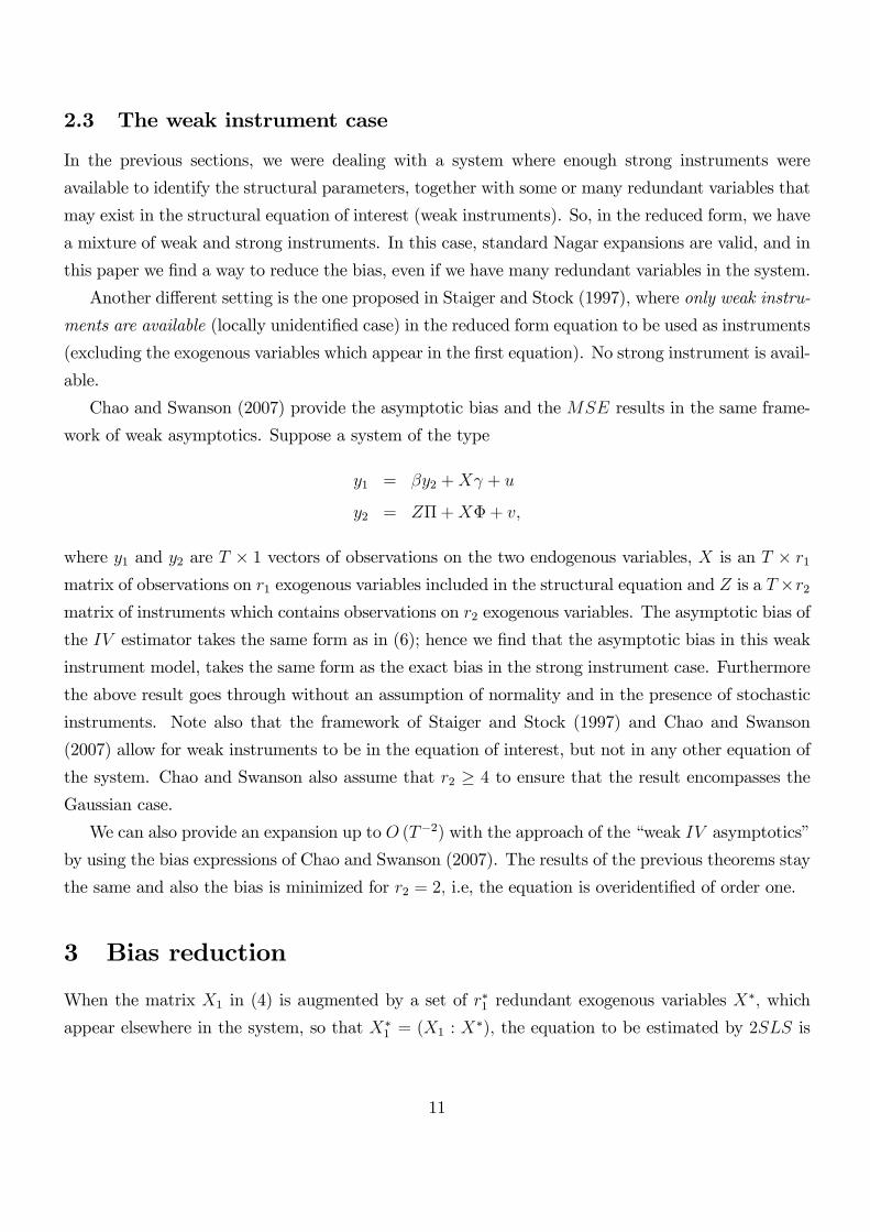
2.3 The weak instrument case

In the previous sections, we were dealing with a system where enough strong instruments were

available to identify the structural parameters, together with some or many redundant variables that

may exist in the structural equation of interest (weak instruments). So, in the reduced form, we have

a mixture of weak and strong instruments. In this case, standard Nagar expansions are valid, and in

this paper we �nd a way to reduce the bias, even if we have many redundant variables in the system.

Another di¤erent setting is the one proposed in Staiger and Stock (1997), where only weak instru-

ments are available (locally unidenti�ed case) in the reduced form equation to be used as instruments

(excluding the exogenous variables which appear in the �rst equation). No strong instrument is avail-

able.

Chao and Swanson (2007) provide the asymptotic bias and the MSE results in the same frame-

work of weak asymptotics. Suppose a system of the type

y1 = �y2 +X + u

y2 = Z�+X� + v;

where y1 and y2 are T � 1 vectors of observations on the two endogenous variables, X is an T � r1matrix of observations on r1 exogenous variables included in the structural equation and Z is a T�r2matrix of instruments which contains observations on r2 exogenous variables. The asymptotic bias of

the IV estimator takes the same form as in (6); hence we �nd that the asymptotic bias in this weak

instrument model, takes the same form as the exact bias in the strong instrument case. Furthermore

the above result goes through without an assumption of normality and in the presence of stochastic

instruments. Note also that the framework of Staiger and Stock (1997) and Chao and Swanson

(2007) allow for weak instruments to be in the equation of interest, but not in any other equation of

the system. Chao and Swanson also assume that r2 � 4 to ensure that the result encompasses theGaussian case.

We can also provide an expansion up to O (T�2) with the approach of the �weak IV asymptotics�

by using the bias expressions of Chao and Swanson (2007). The results of the previous theorems stay

the same and also the bias is minimized for r2 = 2; i.e, the equation is overidenti�ed of order one.

3 Bias reduction

When the matrix X1 in (4) is augmented by a set of r�1 redundant exogenous variables X�; which

appear elsewhere in the system, so that X�1 = (X1 : X

�); the equation to be estimated by 2SLS is

11

now

(7) y1 = Y2� +X1 +X�� + u1;

where � is zero but is estimated as part of the coe¢ cient vector �� = (�0; 0; �0):

The bias in estimating �� takes the same form as (5) except that in the de�nition of Q, X1 is

replaced byX�1 : If r

�1 is chosen so that the notional order of overidenti�cation, de�ned as R�(g1+r1+

r�1) is equal to unity, then the bias of the resulting 2SLS estimator ��; is zero to order T�2: It follows

that �� is unbiased to order T�2 and the result holds whether or not there are weak instruments

in the system as will be discussed below. Of course, the introduction of the redundant variables

changes the variance too. In fact the asymptotic covariance matrix of � is given by limT!1 �2TQ ,

whereas the asymptotic covariance matrix for �� is given by limT!1 �2TQ�; where Q� is obtained

by replacing X1 with X�1 in Q. Hence, the estimator �

� will not be asymptotically e¢ cient. However

if the redundant variables are weak instruments the increase in the small sample variance will be

small and the MSE may be reduced. We can �nd a second order approximation to the variance of

�� from a simple extension of the earlier results of Nagar (1959) given above.

Although the proposed procedure is based on large sample asymptotic analysis, the case is

strengthened by the exact �nite sample results in Section 4 since we have observed there that setting

r2 = 2 minimizes the exact bias for a given value of the concentration parameter although it does not

completely eliminate it. Of course, as we have noted, the introduction of the redundant exogenous

variables alters the value of the concentration parameter so we cannot be certain that the bias is

reduced. However, all our results indicate that bias reduction will be successful.

E¤ectively, we are using in our analysis an �optimal�number of redundant variables for inclusion

in the �rst equation to improve on the �nite sample properties of the 2SLS=IV instrumental variable

estimator of �: By doing so we know that, in the two-equation model, this type of overspeci�cation has

the drawback that it decreases the concentration parameter �0�; so we want to choose the redundant

variables from the weaker instruments. In the de�nition of weak instruments, it is usual to refer to

such instruments as those which make only a small contribution to the concentration parameter

(see eg. Stock, Wright and Yogo (2002) and Davidson and Mackinnon (2006)). So this adds support

for what we do and guides our selection of variables in choosing the redundant set. This is further

discussed in the next section.

A related approach is to commence from the correctly speci�ed equation and achieve the bias

reduction by suitably reducing the number of instruments included at the �rst stage. If the number

of retained instruments at the �rst stage includes the exogenous variables that appear in the correctly

speci�ed equation to be estimated while the total number is such as to make the equation notionally

overidenti�ed of order one, then the resulting IV estimator will also be unbiased to order T�2. An

12

obvious way to choose the instruments to be removed from the �rst stage would be to select the

weakest. We shall consider this approach again in Section 3.1.

We have seen in Section 2 that the limiting bias in the weak instrument model of Staiger and

Stock (1997) and of Chao and Swanson (2007), takes the same form as the exact bias in �nite samples.

Insofar as we can minimize the exact bias by setting r2 = 2; it follows that we also minimize the

limiting bias in the weak instrument case. As a result we can reasonably expect our bias reduction

procedure will work in models even where the weak instrument problem is severe.

We have earlier noted that the existence of moments depends on the �notional�order of overi-

denti�cation. To see why this is so we consider a simple system of 2 endogenous variables as given

in (7), and a reduced form equation

(8) y2 = X�2 + v2;

then the 2SLS estimator of � has the form (y2�Py2)�1 (y2�Py1) ; where P = X (X�X)

�1X��X1 (X01X1)

�1X1�

and rank(P ) = p =rank(X)�rank(X1) : To examine the existence of moments, we can take a look at

the canonical case where the covariance matrix of (u1; v2) is just the identity, and � = 0 = = � = �2:

Then, conditional on y2; the distribution of the 2SLS estimator is N�0; (y2�Py2)

�1� ; so the condi-tional moments all exist, the odd vanish, and the unconditional even moment of order 2r exists only

if E�(y2�Py2)

�r� exists. But y2�Py2 � �2p; so this it exists only for p < 2r; or 2r � p� 1: In the non-canonical case the odd-order moments do not vanish, but the argument is the same. This provides

the intuition of why, by adding redundant exogenous in the system, in this case by altering p; we

alter the notional order of identi�cation and it is this which determines the existence of moments1.

Note that in our bias results, � corresponds to the full vector of parameters so that the bias is

zero to order 1=T 2 for the exogenous coe¢ cient estimators too. This is important because not all

bias corrected estimators proposed in the literature have this quality. For example, the standard

delete-one jackknife in Hahn, Hausman and Kuersteiner (2004) is shown to perform quite well and

it has moments whenever 2SLS has moments. However, the case analyzed does not include any

exogenous variables in the equation that is estimated so no results are given for the jackknife applied

to exogenous coe¢ cient estimators. In fact, a necessary condition for the jackknife to reduce bias is

that the estimator has a bias that is monotonically non-increasing with the sample size. As noted

previously, the bias of the 2SLS estimator of the endogenous variable coe¢ cient is monotonically

non-increasing and so in this case the jackknife satis�es the necessary condition for bias reduction to

be successful. However, Ip and Phillips (1998) show that the same does not apply to the exogenous

coe¢ cient bias. In fact, even the MSE of the 2SLS estimator in this case is not monotonically

non-increasing in the sample size which is a disquieting limitation of the 2SLS method.

1We thank Grant Hillier for providing this simple proof.

13

As noted in Section 2, the Nagar bias approximation is valid under conditional heteroskedasticity

so that we can prove that the bias disappears up to O (T�1) even when conditional heteroskedasticity

is present. The essential requirement is that the disturbances be Gauss Markov which covers a wide

range of generalized-autoregressive conditional heteroskedastic (ARCH=GARCH) processes (see,

e.g. Bollerslev (1986)).

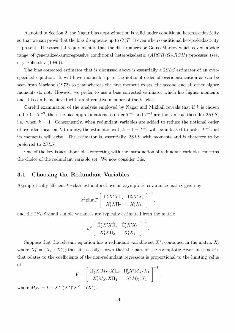
The bias corrected estimator that is discussed above is essentially a 2SLS estimator of an over-

speci�ed equation. It will have moments up to the notional order of overidenti�cation as can be

seen from Mariano (1972) so that whereas the �rst moment exists, the second and all other higher

moments do not. However we prefer to use a bias corrected estimator which has higher moments

and this can be achieved with an alternative member of the k�class.Careful examination of the analysis employed by Nagar and Mikhail reveals that if k is chosen

to be 1� T�3; then the bias approximations to order T�1 and T�2 are the same as those for 2SLS,i.e. when k = 1. Consequently, when redundant variables are added to reduce the notional order

of overidenti�cation L to unity, the estimator with k = 1 � T�3 will be unbiased to order T�2 andits moments will exist. The estimator is, essentially, 2SLS with moments and is therefore to be

preferred to 2SLS.

One of the key issues about bias correcting with the introduction of redundant variables concerns

the choice of the redundant variable set. We now consider this.

3.1 Choosing the Redundant Variables

Asymptotically e¢ cient k�class estimators have an asymptotic covariance matrix given by

�2plimT

"�02X

0X�2 �02X0X1

X 01X�2 X 0

1X1

#�1;

and the 2SLS small sample variances are typically estimated from the matrix

�2

"�02X

0X�2 �02X0X1

X 01X�2 X 0

1X1

#�1:

Suppose that the relevant equation has a redundant variable set X�, contained in the matrix X;

where X�1 = (X1 : X

�); then it is easily shown that the part of the asymptotic covariance matrix

that relates to the coe¢ cients of the non-redundant regressors is proportional to the limiting value

of

V =

"�02X

0MX�X�2 �02X0MX�X1

X 01MX�X�2 X 0

1MX�X1

#�1;

where MX� = I �X� [(X�)0X�]�1 (X�)0:

14

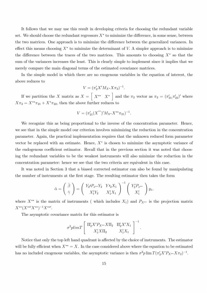
It follows that we may use this result in developing criteria for choosing the redundant variable

set. We should choose the redundant regressorsX� to minimize the di¤erence, in some sense, between

the two matrices. One approach is to minimize the di¤erence between the generalized variances. In

e¤ect this means choosing X� to minimize the determinant of V: A simpler approach is to minimize

the di¤erence between the traces of the two matrices. This amounts to choosing X� so that the

sum of the variances increases the least. This is clearly simple to implement since it implies that we

merely compare the main diagonal terms of the estimated covariance matrices.

In the simple model in which there are no exogenous variables in the equation of interest, the

above reduces to

V = (�02X0MX�X�2)

�1:

If we partition the X matrix as X =hX�� X�

iand the �2 vector as �2 = (�021:�

022)

0 where

X�2 = X���21 +X

��22; then the above further reduces to

V = (�021(X��)0MX�X���21)

�1:

We recognize this as being proportional to the inverse of the concentration parameter. Hence,

we see that in the simple model our criterion involves minimizing the reduction in the concentration

parameter. Again, the practical implementation requires that the unknown reduced form parameter

vector be replaced with an estimate. Hence, X� is chosen to minimize the asymptotic variance of

the endogenous coe¢ cient estimator. Recall that in the previous section it was noted that choos-

ing the redundant variables to be the weakest instruments will also minimize the reduction in the

concentration parameter: hence we see that the two criteria are equivalent in this case.

It was noted in Section 3 that a biased corrected estimator can also be found by manipulating

the number of instruments at the �rst stage. The resulting estimator then takes the form

� =

�

!=

Y20Px��Y2 Y 02X1

X 01Y2 X 0

1X1

!�1 Y 02Px��

X 01

!y1;

where X�� is the matrix of instruments ( which includes X1) and PX�� is the projection matrix

X��(X��0X��)�1X��0:

The asymptotic covariance matrix for this estimator is

�2plimT

"�02X

0PX��X�2 �02X0X1

X 01X�2 X 0

1X1

#�1:

Notice that only the top left hand quadrant is a¤ected by the choice of instruments. The estimator

will be fully e¢ cient whenX�� = X. In the case considered above where the equation to be estimated

has no included exogenous variables, the asymptotic variance is then �2p limT (�02X0PX��X�2)

�1:

15

It does not appear possible to show that either estimator dominates the other on aMSE criterion.

However, it can easily be shown that when X� is orthogonal to X��; i:e; the redundant variables in

the estimated equation are orthogonal to all the other instruments, and whenever the alternative

method is used it is the X�variables which are excluded from the �rst stage, the two approaches lead

to exactly the same estimators. Some simulations have shown that the two estimators give quite

similar results. One reason for preferring the redundant variable estimator is that it is simply a

special case of 2SLS (or k�class) about which a good deal is known, including its exact properties insimple cases. In what follows we shall be primarily concerned with the redundant variable method.

Later in the paper we shall examine the properties of the redundant variable estimator in a

series of Monte Carlo experiments but �rst we consider an alternative approach to bias correction

by combining k�class estimators.

4 A new estimator as a linear combination of k-class esti-

mators with k < 1

In this section we develop a new estimator as a linear combination of k�class estimators with k < 1.As we shall see the new estimator has all higher moments and is unbiased to order T�1:

To proceed we shall denote the estimator when k = 1� T�3 as b�k1 and the estimator for whichk = 1� T�1 as b�k2. According to (5), the bias of �k1up to T�1takes the form

Bias (b�k1) = (L� 1)Qq;and b�k2 ;the k�class estimator for which k = 1� 1

T; has bias given by

Bias (b�k2) = LQq:It follows that the linear combination of b�k1 and b�k2 given by

b�k3 = Lb�k1 � (L� 1)b�k2(9)

= b�k1 + (L� 1)(b�k1 � b�k2)(10)

is unbiased to order T�1:This is the combined estimator.

It is of interest that the combined estimator is approximately unbiased under much less restricted

conditions than those imposed by Nagar (1959) as are the estimators considered in the previous

section. The 2SLS case is considered in Phillips (2000, 2007) where it was shown that the bias

approximation holds even in the presence of ARCH=GARCH disturbances while Phillips (1997)

had extended the result to cover the general k�class estimator. An earlier attempt to reduce bias by

16

combining k�class estimators is given in Sawa (1972) who showed that a linear combination of OLSand 2SLS can be found to yield an estimator which is unbiased to order �2:However the estimator

is not unbiased to order T�1 and has been found to perform relatively poorly in some cases. In fact,

the O(T�1) bias approximation for OLS di¤ers considerably from the O(�2) approximation as can

be seen in Kiviet and Phillips (1996). A further disadvantage is that a variance approximation is not

available.

The next Theorem shows how the combined estimator may have smaller MSE than 2SLS for

systems that have, at least, a moderate degree of overidenti�cation. That means that when we have a

reasonable number of instruments (upwards of 7), our combined estimator will not only be unbiased

to order T�1, but also it will improve on �k1 in terms of MSE. Moreover, note that the combined

estimator is always unbiased to order T�1 even if we have added irrelevant variables in any part of

the system (as Hale, Mariano and Ramage (1980) point out). This also includes the case where we

have many weak instruments in the system.

Theorem 1 In the model of (1) and under Assumption A in Section 2, the di¤erence to order T�2

between the mean squared error of the combined estimator b�k3 and that of the k�class estimator forwhich k = 1� T�3, b�k1 ; is given by

E(b�k1 � �)(b�k1 � �)0 � E(b�k3 � �)(b�k3 � �)0= �2(L� 1)[(L� 7)QC1Q� 2QC2Q� 2(tr(C1Q)Q�QC1Q)] + o(T�2):

The proof of this Theorem is given in the Appendix where it is shown that the Nagar expansion

of the estimation error of the combined estimator b�k3 to Op(T �32 ) is exactly the same as that for the

Nagar unbiased estimator for which k = 1 + L�1T. Second moment approximations are based only

on terms up to Op(T�32 )so that the second moment approximation for the combined estimator will

be the same as that of the Nagar unbiased estimator to order T�2:Hence the combined estimator is

essentially the same as Nagar�s unbiased estimator with all necessary moments.

It is of interest to compare the combined estimator with a bias corrected estimator proposed by

Donald and Newey (2001, page 1164). Their B2SLS estimator is given as

� =�Z 0PXZ � �� Z 0Z)

��1(Z 0PX y1 � �� Z 0y1);

which is clearly a k�class estimator for which (1�k)k

= ���: Solving for k yields (1� k) + k�� = 0 or1 = k(1� ��) which gives k = 1

(1���) : Now Donald and Newey (2001) state that�� = (R� r1 � 2)=T

( in out notation) so that k = 11�(R�r1�2)=T = 1 +

(R�r1�2)=T1�(R�r1�2)=T > 1:

Nagar�s unbiased estimator for which k = 1 + (L � 1)=T is not the same as the Donald-Neweyestimator. However to order T�1 the Donald and Newey (2001) estimator has k = 1 + (R � r1 �

17

2)=T; which coincides with Nagar�s estimator when there is only one endogenous regressor but not

otherwise. Therefore, the unbiasedness of the Donald and Newey (2001) estimator in the context of

more than 1 endogenous variables in the system is not a trivial extension. Moreover, the Donald and

Newey estimator is momentless for the case of one endogenous regressor . One of the main novelties

of our paper, is that we present an unbiased estimator to order T�1 in the setting of any number of

endogenous variables and that allows for the existence of any number of irrelevant variables in the

system. Moreover, our estimator has moments when dealing with the k�class where k < 1.The precise value for L at which the result in Theorem 1 above is positive semi-de�nite so that the

MSE of the combined estimator is less than that of 2SLS; depends upon the relationship between

QC1Q and QC2Q. This is especially so in the two equation model where tr(C1Q)Q = QC1Q:However

it is to be expected that QC1Q � QC2Q , especially when the simultaneity is strong , so that the

combined estimator is preferred on a MSE criterion for L > 7: Of course, when L = 1 the MSE

of 2SLS does not exist and the combined estimator is preferred. In this case b�k3 = b�k1 ; thus thecombined estimator reduces to the k�class estimator for which k = 1� T�3:Although we show thatthe combined estimator only dominates in other cases for L = 0 and for values of L > 7, it should

be noted that the combined estimator is always approximately unbiased, has all necessary moments

and may be preferred in cases where biases are large even if it it is not optimal on a MSE criterion.

Note that the Chao and Swanson (2007) bias correction procedure does not work very well when

the number of excluded regressors is less than 11 (see Chao and Swanson (2007), Table 2) while we

have a very simple procedure that is unbiased up to T�1 for any number of excluded regressors. Our

combined estimator, which does not assume that all instruments are weak, will work particularly well

in the case of many (weak) instruments and moderate number of (weak) instruments. The result is

the same regardless of whether our instruments are weak or strong and the unbiasedness result holds

under possible overspeci�cation in terms of including irrelevant variables in other equations. Note

also that Chao and Swanson (2007) need a correctly speci�ed system, while our combined estimator

will be unbiased up to T�1 even if we have irrelevant exogenous variables in any part of the system.

As Hansen, Hausman and Newey (2008) point out, there are many papers that need in practice to

use a moderate/large number of instruments, and Angrist and Krueger (1991) is an example where

a large number of instruments is used.

As a �nal remark, note that in the case L = 0, the combined estimator reduces to the k�classestimator with k = 1 � T�1. This has moments and clearly dominates 2SLS and the k = 1 � T�3

estimator on a MSE criterion in this situation. Actually this is quite obvious since the variance of

the k�class will decline as k is reduced and so the estimator with k = 1� T�1 will have a smaller

variance while at the same time it has a zero bias to order T�1 when L = 0: This estimator is

of considerable importance since it has higher moments when 2SLS does not yet, as noted in the

18

introduction, and it is very commonly found in practice.

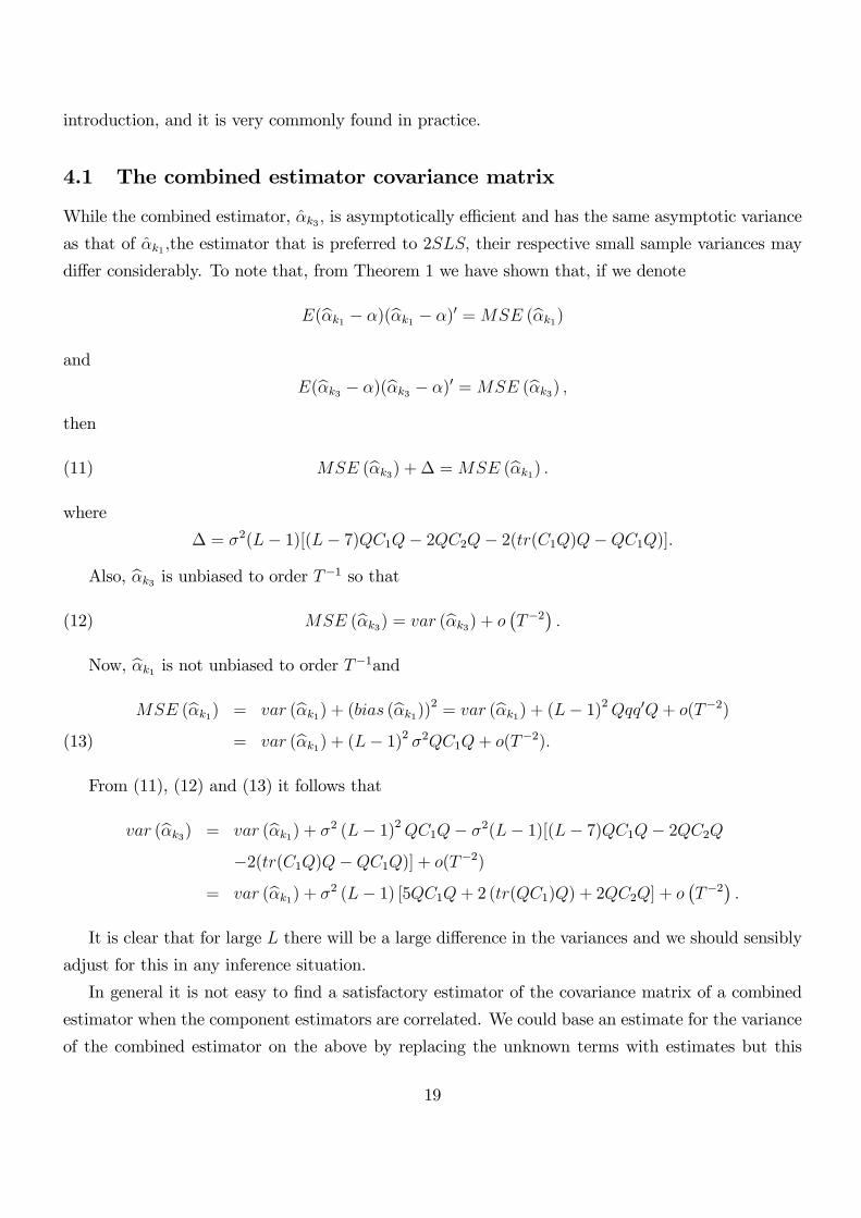
4.1 The combined estimator covariance matrix

While the combined estimator, �k3 ; is asymptotically e¢ cient and has the same asymptotic variance

as that of �k1 ;the estimator that is preferred to 2SLS; their respective small sample variances may

di¤er considerably. To note that, from Theorem 1 we have shown that, if we denote

E(b�k1 � �)(b�k1 � �)0 =MSE (b�k1)and

E(b�k3 � �)(b�k3 � �)0 =MSE (b�k3) ;then

(11) MSE (b�k3) + � =MSE (b�k1) :where

� = �2(L� 1)[(L� 7)QC1Q� 2QC2Q� 2(tr(C1Q)Q�QC1Q)]:

Also, b�k3 is unbiased to order T�1 so that(12) MSE (b�k3) = var (b�k3) + o �T�2� :Now, b�k1 is not unbiased to order T�1and

MSE (b�k1) = var (b�k1) + (bias (b�k1))2 = var (b�k1) + (L� 1)2Qqq0Q+ o(T�2)= var (b�k1) + (L� 1)2 �2QC1Q+ o(T�2):(13)

From (11), (12) and (13) it follows that

var (b�k3) = var (b�k1) + �2 (L� 1)2QC1Q� �2(L� 1)[(L� 7)QC1Q� 2QC2Q�2(tr(C1Q)Q�QC1Q)] + o(T�2)

= var (b�k1) + �2 (L� 1) [5QC1Q+ 2 (tr(QC1)Q) + 2QC2Q] + o �T�2� :It is clear that for large L there will be a large di¤erence in the variances and we should sensibly

adjust for this in any inference situation.

In general it is not easy to �nd a satisfactory estimator of the covariance matrix of a combined

estimator when the component estimators are correlated. We could base an estimate for the variance

of the combined estimator on the above by replacing the unknown terms with estimates but this

19

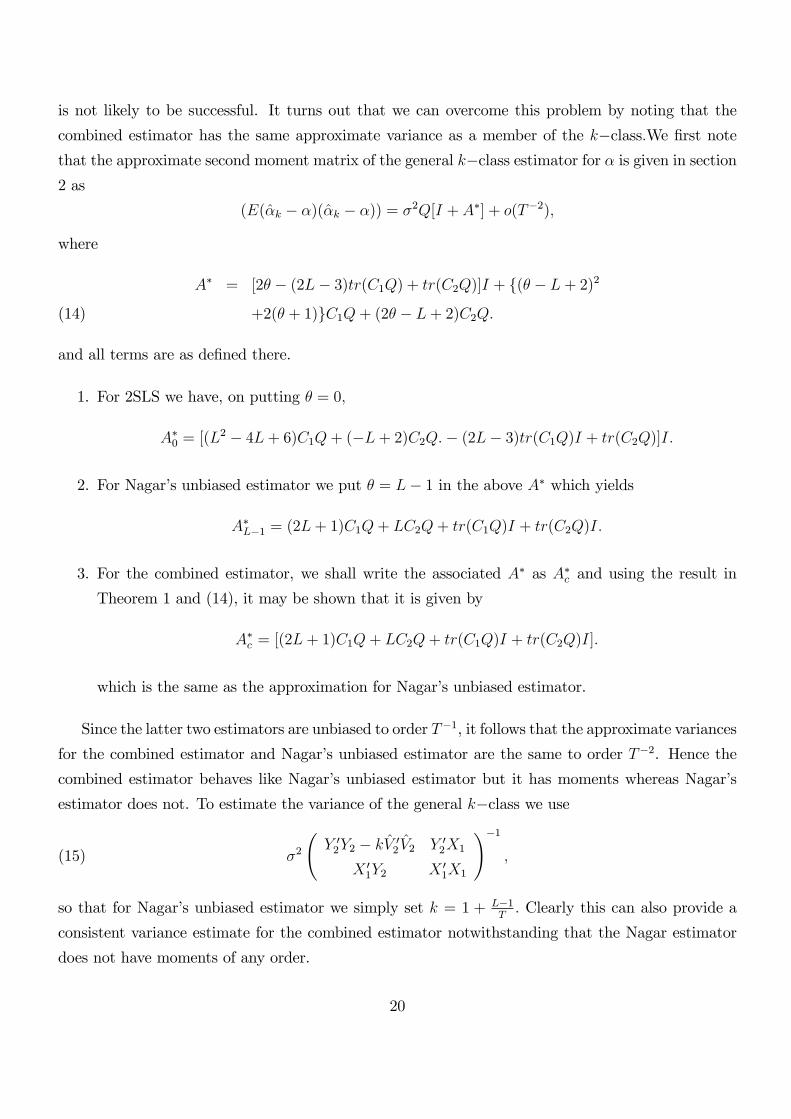
is not likely to be successful. It turns out that we can overcome this problem by noting that the

combined estimator has the same approximate variance as a member of the k�class:We �rst notethat the approximate second moment matrix of the general k�class estimator for � is given in section2 as

(E(�k � �)(�k � �)) = �2Q[I + A�] + o(T�2);

where

A� = [2� � (2L� 3)tr(C1Q) + tr(C2Q)]I + f(� � L+ 2)2

+2(� + 1)gC1Q+ (2� � L+ 2)C2Q:(14)

and all terms are as de�ned there.

1. For 2SLS we have, on putting � = 0;

A�0 = [(L2 � 4L+ 6)C1Q+ (�L+ 2)C2Q:� (2L� 3)tr(C1Q)I + tr(C2Q)]I:

2. For Nagar�s unbiased estimator we put � = L� 1 in the above A� which yields

A�L�1 = (2L+ 1)C1Q+ LC2Q+ tr(C1Q)I + tr(C2Q)I:

3. For the combined estimator, we shall write the associated A� as A�c and using the result in

Theorem 1 and (14), it may be shown that it is given by

A�c = [(2L+ 1)C1Q+ LC2Q+ tr(C1Q)I + tr(C2Q)I]:

which is the same as the approximation for Nagar�s unbiased estimator.

Since the latter two estimators are unbiased to order T�1, it follows that the approximate variances

for the combined estimator and Nagar�s unbiased estimator are the same to order T�2. Hence the

combined estimator behaves like Nagar�s unbiased estimator but it has moments whereas Nagar�s

estimator does not. To estimate the variance of the general k�class we use

(15) �2

Y 02Y2 � kV 02 V2 Y 02X1

X 01Y2 X 0

1X1

!�1;

so that for Nagar�s unbiased estimator we simply set k = 1 + L�1T: Clearly this can also provide a

consistent variance estimate for the combined estimator notwithstanding that the Nagar estimator

does not have moments of any order.

20

5 Simulations

5.1 Results for the redundant variable estimator

We show in this section how our procedure works in practice. Table 1 provides simulations for a

sample of size of 100 observations based on 5000 replications, and the structure we consider is of the

form

y1t = �1y2t + x01t + u1t(16)

y2t = �2y1t + x0t 1 + u2t

y2t = x0t�2 + v2t:(17)

In many of our simulations, was chosen to be zero so that the �rst equation in (16) did not

contain any non-redundant exogenous variables. However, in some of our experiments (EXP ) we in-

cluded one or more non-redundant exogenous variables whereupon had some non-zero components.

Any redundant variables added to the �rst equation, were also included in the second equation. Only

the �rst equation is estimated.

In matrix notation the system may be written as

(18) Y B�+X��+ U = 0:

In all our experiments the X matrix contains a �rst column of ones, while the other exoge-

nous variables are generated as normal random variables with a mean zero and variance 10. The

endogenous coe¢ cient matrix was chosen as

B�=

�1 0:267

0:222 �1

!;

in all experiments. Note that the coe¢ cient of the endogenous regressor, �1; which is the object of

interest in our �rst �ve experiments (Table 1), has the value 0:222. The experiments di¤er through

changing the coe¢ cient matrix of the exogenous coe¢ cients, �: In the �rst �ve experiments this

is e¤ected by changing the exogenous coe¢ cients in the second equation only since no exogenous

coe¢ cients appear in the �rst equation. The disturbances are generated as the product of a 100� 2

matrix ofN(0; 1) times a Cholesky decomposition matrix (C ). This was chosen as C =

112 �1�1 4

!

in all experiments except experiment 2 where it was changed to C =

10 �1�1 4

!:

The model has been estimated �rst by 2SLS and then by 2SLS with redundant exogenous

regressors. We show the consequences of including exogenous variables that act as weak or strong

21

instruments, and we consider di¤erent structures in the disturbances. We give details of the individual

experiments below. Note also that the standard error (se) of 2SLS when we add two redundants

does not exist, and that is why we also report the interquartile range (IR).

Moreover, we also give the results for an alternative k�class estimators: k = 1�T�3 which yieldsb�k1 : This k�class estimators behaves very much like 2SLS �i.e. b�1� but the variance will existwhen the system is overidenti�ed of order 1.

Experiment 1

� =

0 0 0 0

1:47 0:246 0:136 0:043

!; C =

112 �1�1 4

!;

Here the equation speci�ed contains two endogenous variables and no exogenous ones. There are

four exogenous variables in the second equation so that the �rst equation is overidenti�ed of order

three.

Notice that the fourth coe¢ cient in � is numerically small. This corresponds to a weak instrument.

To create a situation where the �rst equation is overidenti�ed of order one so that the 2SLS estimator

is unbiased to order T�2; we shall need to augment the �rst equation with two redundant variables.

There are four variables to choose from. In the �rst experiment the the augmentation proceeds in

two stages. First we introduce variables three and four which are the weaker instruments. Then an

alternative ordering was tried with variables two and three. Thus now one of the redundant variables

is a relatively strong instrument. A comparison of these two cases will show the di¤erent e¤ects of

redundant weak and strong instruments.

As our theory predicts, the bias is drastically reduced when either pair of exogenous variables

are added as redundant, but it is the weaker instruments that increase the standard error the least.

Moreover, if we add three exogenous variables then the redundant 2SLS estimator does not have

moments of any order and it creates outliers in our simulations.

Experiment 2

� =

0 0 0 0

0:5 0:100 0:036 0:043

!, C =

10 �1�1 4

!:

Here the coe¢ cients of the � matrix are di¤erent to those in experiment 1 and the structural

disturbance in the �rst equation is much smaller. The third and fourth coe¢ cients are small too

so now there are two instruments that are relatively weak. In this experiment we choose variables

three and four for the redundant pair and so in this case the augmenting variables are both relatively

weak. Again the bias is drastically reduced.

22

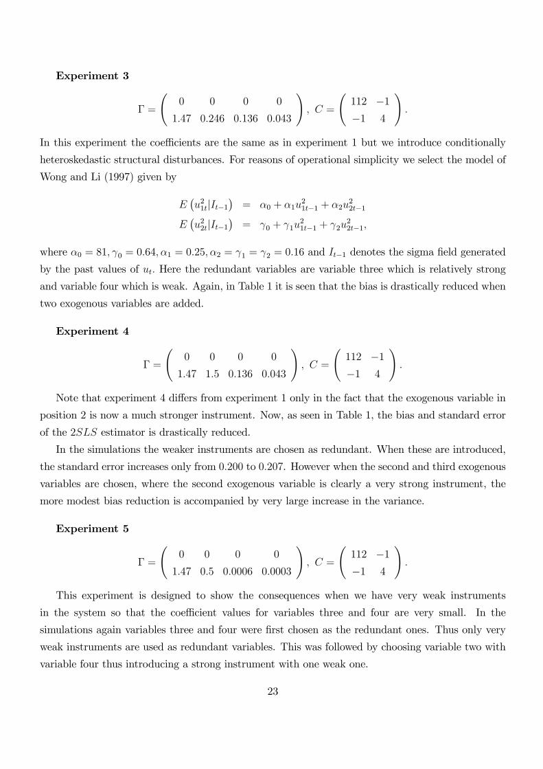
Experiment 3

� =

0 0 0 0

1:47 0:246 0:136 0:043

!; C =

112 �1�1 4

!:

In this experiment the coe¢ cients are the same as in experiment 1 but we introduce conditionally

heteroskedastic structural disturbances. For reasons of operational simplicity we select the model of

Wong and Li (1997) given by

E�u21tjIt�1

�= �0 + �1u

21t�1 + �2u

22t�1

E�u22tjIt�1

�= 0 + 1u

21t�1 + 2u

22t�1;

where �0 = 81; 0 = 0:64; �1 = 0:25; �2 = 1 = 2 = 0:16 and It�1 denotes the sigma �eld generated

by the past values of ut: Here the redundant variables are variable three which is relatively strong

and variable four which is weak. Again, in Table 1 it is seen that the bias is drastically reduced when

two exogenous variables are added.

Experiment 4

� =

0 0 0 0

1:47 1:5 0:136 0:043

!; C =

112 �1�1 4

!:

Note that experiment 4 di¤ers from experiment 1 only in the fact that the exogenous variable in

position 2 is now a much stronger instrument. Now, as seen in Table 1, the bias and standard error

of the 2SLS estimator is drastically reduced.

In the simulations the weaker instruments are chosen as redundant. When these are introduced,

the standard error increases only from 0:200 to 0:207. However when the second and third exogenous

variables are chosen, where the second exogenous variable is clearly a very strong instrument, the

more modest bias reduction is accompanied by very large increase in the variance.

Experiment 5

� =

0 0 0 0

1:47 0:5 0:0006 0:0003

!; C =

112 �1�1 4

!:

This experiment is designed to show the consequences when we have very weak instruments

in the system so that the coe¢ cient values for variables three and four are very small. In the

simulations again variables three and four were �rst chosen as the redundant ones. Thus only very

weak instruments are used as redundant variables. This was followed by choosing variable two with

variable four thus introducing a strong instrument with one weak one.

23

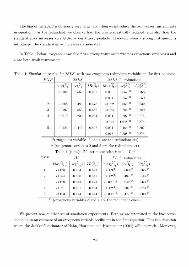
The bias of the 2SLS is obviously very large, and when we introduce the two weakest instruments

in equation 1 as the redundant, we observe how the bias is drastically reduced, and also, how the

standard error increases very little, as our theory predicts. However, when a strong instrument is

introduced, the standard error increases considerably.

In Table 1 below, exogenous variable 2 is a strong instrument whereas exogenous variables 3 and

4 are both weak instruments.

Table 1: Simulation results for 2SLS, with two exogenous redundant variables in the �rst equation

EXP 2SLS 2SLS, 2�redundantsbias(b�1) se(b�1) IR(b�1) bias(b��1) se(b��1) IR(b��1)

1 -0.182 0.566 0.667 0.009 0.657(1) 0.766

0.004 0.757(2) 0.859

2 -0.088 0.483 0.578 -0.022 0.660(1) 0.632

3 -0.197 0.553 0.682 -0.024 0.784(1) 0.789

4 -0.019 0.200 0.264 0.001 0.207(1) 0.274

-0.014 1.648(2) 0.874

5 -0.123 0.442 0.547 0.001 0.484(1) 0.597

0.015 0.808(2) 0.874(1)(exogenous variables 3 and 4 are the redundant set);(2)(exogenous variables 2 and 3 are the redundant set)

Table 1 (cont.): IV�estimator with k = 1� T�3

EXP IV IV , 2�redundantsbias(b�k1) se(b�k1) IR(b�k1) bias(b��k1) se(b��k1) IR(b��k1)

1 -0.178 0.554 0.693 0.009(1) 0.660(1) 0.765(1)

2 -0.084 0.450 0.541 0.002(1) 0.487(1) 0.545(1)

3 -0.178 0.543 0.623 -0.020(1) 0.942(1) 0.760(1)

4 -0.021 0.201 0.264 0.002(1) 0.207(1) 0.270(1)

5 -0.123 0.444 0.544 -0.008(1) 0.477(1) 0.600(1)

(1)(exogenous variables 3 and 4 are the redundant ones).

We present now another set of simulation experiments. Here we are interested in the bias corre-

sponding to an estimate of an exogenous variable coe¢ cient in the �rst equation. This is a situation

where the Jackknife estimator of Hahn, Hausman and Kuersteiner (2004) will not work . Moreover,

24

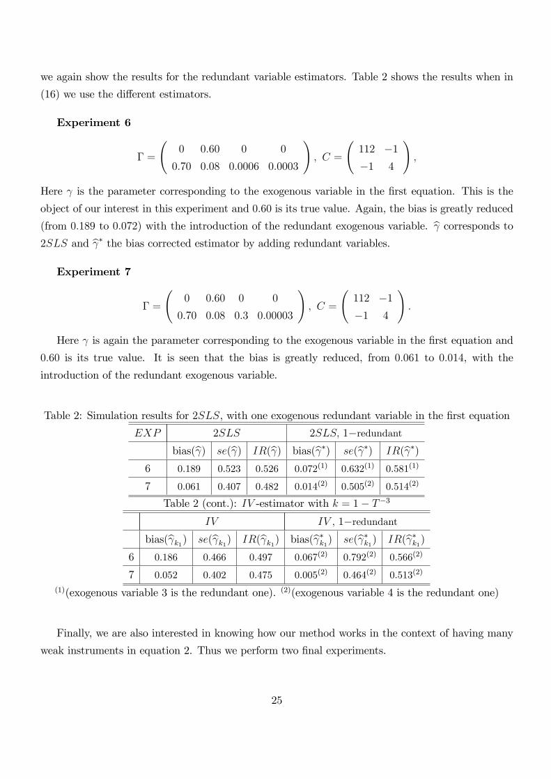
we again show the results for the redundant variable estimators. Table 2 shows the results when in

(16) we use the di¤erent estimators.

Experiment 6

� =

0 0:60 0 0

0:70 0:08 0:0006 0:0003

!; C =

112 �1�1 4

!;

Here is the parameter corresponding to the exogenous variable in the �rst equation. This is the

object of our interest in this experiment and 0:60 is its true value. Again, the bias is greatly reduced

(from 0:189 to 0:072) with the introduction of the redundant exogenous variable. b corresponds to2SLS and b � the bias corrected estimator by adding redundant variables.Experiment 7

� =

0 0:60 0 0

0:70 0:08 0:3 0:00003

!; C =

112 �1�1 4

!:

Here is again the parameter corresponding to the exogenous variable in the �rst equation and

0:60 is its true value. It is seen that the bias is greatly reduced, from 0:061 to 0:014, with the

introduction of the redundant exogenous variable.

Table 2: Simulation results for 2SLS, with one exogenous redundant variable in the �rst equation

EXP 2SLS 2SLS; 1�redundantbias(b ) se(b ) IR(b ) bias(b �) se(b �) IR(b �)

6 0.189 0.523 0.526 0.072(1) 0.632(1) 0.581(1)

7 0.061 0.407 0.482 0.014(2) 0.505(2) 0.514(2)

Table 2 (cont.): IV -estimator with k = 1� T�3

IV IV , 1�redundantbias(b k1) se(b k1) IR(b k1) bias(b �k1) se(b �k1) IR(b �k1)

6 0.186 0.466 0.497 0.067(2) 0.792(2) 0.566(2)

7 0.052 0.402 0.475 0.005(2) 0.464(2) 0.513(2)

(1)(exogenous variable 3 is the redundant one). (2)(exogenous variable 4 is the redundant one)

Finally, we are also interested in knowing how our method works in the context of having many

weak instruments in equation 2. Thus we perform two �nal experiments.

25

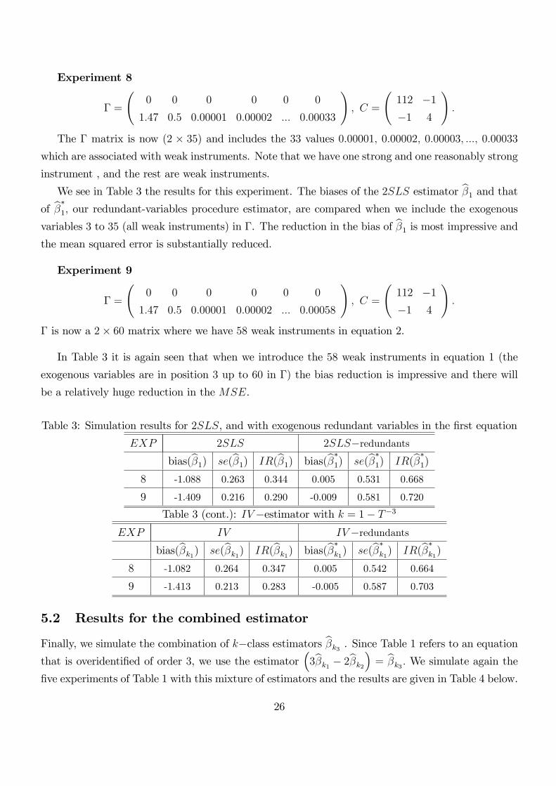
Experiment 8

� =

0 0 0 0 0 0

1:47 0:5 0:00001 0:00002 ::: 0:00033

!; C =

112 �1�1 4

!:

The � matrix is now (2 � 35) and includes the 33 values 0:00001; 0:00002; 0:00003; :::; 0:00033which are associated with weak instruments. Note that we have one strong and one reasonably strong

instrument , and the rest are weak instruments.

We see in Table 3 the results for this experiment. The biases of the 2SLS estimator b�1 and thatof b��1; our redundant-variables procedure estimator, are compared when we include the exogenousvariables 3 to 35 (all weak instruments) in �. The reduction in the bias of b�1 is most impressive andthe mean squared error is substantially reduced.

Experiment 9

� =

0 0 0 0 0 0

1:47 0:5 0:00001 0:00002 ::: 0:00058

!; C =

112 �1�1 4

!:

� is now a 2� 60 matrix where we have 58 weak instruments in equation 2.

In Table 3 it is again seen that when we introduce the 58 weak instruments in equation 1 (the

exogenous variables are in position 3 up to 60 in �) the bias reduction is impressive and there will

be a relatively huge reduction in the MSE.

Table 3: Simulation results for 2SLS, and with exogenous redundant variables in the �rst equation

EXP 2SLS 2SLS�redundantsbias(b�1) se(b�1) IR(b�1) bias(b��1) se(b��1) IR(b��1)

8 -1.088 0.263 0.344 0.005 0.531 0.668

9 -1.409 0.216 0.290 -0.009 0.581 0.720

Table 3 (cont.): IV�estimator with k = 1� T�3

EXP IV IV�redundantsbias(b�k1) se(b�k1) IR(b�k1) bias(b��k1) se(b��k1) IR(b��k1)

8 -1.082 0.264 0.347 0.005 0.542 0.664

9 -1.413 0.213 0.283 -0.005 0.587 0.703

5.2 Results for the combined estimator

Finally, we simulate the combination of k�class estimators b�k3 . Since Table 1 refers to an equationthat is overidenti�ed of order 3, we use the estimator

�3b�k1 � 2b�k2� = b�k3 : We simulate again the

�ve experiments of Table 1 with this mixture of estimators and the results are given in Table 4 below.

26

Table 4: IV�estimator b�k3EXP IV

bias(b�k3) se(b�k3) IR(b�k3)1 -0.028 0.658 0.760

2 -0.024 0.620 0.656

3 -0.039 0.708 0.748

4 -0.002 0.205 0.271

5 -0.016 0.497 0.617

8 -0.703 0.390 0.513

9 -0.971 0.292 0.381

By comparing the results of Table 1 for the �rst �ve experiments with those in Table 4, we see the

clear advantage this combined estimator has in relation to the traditional 2SLS estimator mainly in

terms of the biases. In the experiments where the weakest instruments were used for the redundant

set, the redundant variable estimator compares favorably with the combined estimator in terms of the

standard deviation and is, as expected, generally less biased. However when the redundant variables

include at least one strong instrument the redundant variable estimator, while continuing to have

very small bias, also su¤ered an increase in the standard deviation, see especially Experiment 4,

indicating the need for caution in using the estimator. Of course, in practice, it is to be expected

that the estimated variance would provide a warning against using the estimator.

We also show the behavior of the combined estimator for experiments 8 and 9. In these last two

cases, we set b�k3 = �34b�k1 � 33b�k2� and b�k3 = �59b�k1 � 58b�k2� respectively.In these experiments we have L >> 8, and as our theory predicts, the combined estimator is

clearly superior in terms of MSE to 2SLS. However the estimator is still very badly biased even

though the bias of order T�1 has been removed. We also note that in this case, the redundant-variable

method yielded a very small bias.

At �rst sight it is surprising that the bias of the combined estimator is so large. However,

examining the higher order bias approximation in Section 2.1 for 2SLS, we see that the bias term of

order T�2 will be large for large L and this will apply to the combined estimator also. Whereas in

many cases the bias term of order T�2 is relatively small, it is not when there are many instruments.

Even when L � 8 (see experiments 1 � 5), there are some cases where it is advisable in practiceto calculate both 2SLS and our combined estimator and to compare the point estimates for the

econometrician to uncover large biases.

. In the simulations of Hansen, Hausman and Newey (2008) and Chao and Swanson (2007), it

is possible to see that LIML, Fuller or other estimators, may not be median unbiased or unbiased

27

in some situations and it is here where our proposal is useful. As Davidson and Mackinnon (2006)

concluded, there is no clear advantage in using LIML or 2SLS in practice (mainly in situations

such as experiments 8 and 9 where we have many weak instruments). Here we �nd a case where

our combined estimator generally improves on 2SLS in terms of MSE when L � 8; and where

the bias correction works when there are redundant variables in any equation of the simultaneous

equation system whatever the order of identi�cation. Therefore, if L < 8 the researcher should useour combined estimator instead of 2SLS; and even if L < 8; in some cases such as experiments 1 and

5, we can see by comparing Tables 1 and 4, that the bias correction is so large than the researcher

may still consider it useful to use the combined estimator and compare it with 2SLS.

Moreover, in the case of many instruments, the bias correction through the introduction of redun-

dant variables produces a much larger bias reduction than our combined estimator. So in practice, it

is advisable in the case of many instruments (more than 7) to compare also our combined estimator

(clearly superior to the estimator with k = 1� T�3) with the redundant variable estimator.Finally, in order to check our Theorem 1, we repeat Experiment 9 but instead of including 58

instruments we only include just 10 weak instruments with coe¢ cients 0:00001; 0:00002; 0:00003; :::;

0:00010: This is what we call Experiment 10. Our Theorem 1 predicts that from the number of

instruments 8 onwards, the combined estimator should improve on MSE in relation to 2SLS. We

show in Table 5 below that when we have 10 weak instruments, the combined estimator does indeed

improve considerably on MSE in relation to 2SLS. The same situation is seen in Experiments 8

and 9 when we compare Tables 3 and 4. Thus the combined estimator improves theMSE in relation

to 2SLS in a very important way. The gains that we can get in terms of a reduced MSE from the

combined estimator versus 2SLS are very impressive.

Table 5: Simulation results for 2SLS, and with the combined estimator with 10 weak instruments.�11b�k1 � 10b�k2� = b�k3 :

EXP 2SLS combined-IV

bias(b�1) se(b�1) MSE(b�1) bias(b�k3) se(b�k3) MSE(b�k3)10 -0.485 0.358 0.363 -0.143 0.506 0.277

6 An empirical application

In this section we consider an application of bias correction in a simple case and we focus on the

combined estimator which is likely to be of particular interest in practical cases.

One main advantage of our combined estimator is that it is very easy to compute. As is seen in

(10), it simply requires the computation of two k�class estimators for k = 1�T�1 and k = 1�T�3:

28

The STATA package 2 has a module that implements straightforwardly k-class estimators3 written

by Baum, Scha¤er and Stillman (2008)4. To compute the variance of our combined estimator, we

can simply refer to (15), from where we �nd that our combined estimator has an asymptotic variance

equivalent to the k-class estimator with k = 1 + L�1T:

We are interested in analyzing the permanent income hypothesis, and for this purpose, we focus

on equation (16.35) in Example 16.7 in Wooldridge (2008, page 563) where, following Campbell and

Mankiw (1990), we can specify

(19) gct = �0 + �1gyt + �2r3t + ut;

where gct is the annual growth in real per capita consumption (excluding durables), gyt is the growth

in real disposable income and r3t is the (ex post) real interest rate as measured by the return on

three-month T-bill rates.

The hypothesis of interest is that the pure form of the permanent income hypothesis states that

�1 = �2 = 0: Campbell and Mankiw (1990) argue that �1 is positive if some fraction of the population

consumes current income instead of permanent income. And the permanent income hypothesis theory

with a nonconstant real interest rate implies that �2 > 0:

We use the same dataset as in Example 16.7 in Wooldridge (2008, page 563). We use the

annual data from 1959 through 1995 given in CONSUMP.RAW to estimate the equation given by

(19) and the results are given in Table 6. The two endogenous variables are gyt and r3t: Since

a full three-equation model is not speci�ed the choice of instrumental variables is ad hoc and in

equation (16.35), Wooldridge uses as instruments gct�1, gyt�1 and r3t�1 although the full model

is not necessarily dynamic:We report the results when we apply the OLS and 2SLS estimators in

rows (3) and (4) and the corresponding standard errors in parenthesis. These corresponds to the

same reported outcomes in Wooldridge (2008, Example 16.7). From row (4), we can check how the

pure form of the permanent income hypothesis is strongly rejected because the coe¢ cient on gyt is

economically large and statistically signi�cant. The coe¢ cient on the real interest rate is very small

and statistically insigni�cant. Campbell and Mankiw (1990) use di¤erent lags as instruments, so

in order to con�rm these results, we apply in row (5) 2SLS when the instruments are gct�1, gyt�1,

r3t�1; gct�2, gyt�2, r3t�2; gct�3, gyt�3 and r3t�3: The results when we compare rows (4) and (5) are

very similar except that the estimated coe¢ cient on gyt increases slightly from 0.5904 to 0.6153, and

as it is very usual (see for example Wooldridge (2008, Example 15.8)) the standard error of the 2SLS

2see http://www.stata.com/3IVREG2 is a STATA module available at http://ideas.repec.org/c/boc/bocode/s425401.html4We are very grateful to Je¤ Wooldridge for pointing out about the existence of this STATA module, and how

our estimator can be easily computed in STATA. We are also in debt with Je¤ Wooldridge for all his comments and

suggestions that we have obtained about this empirical application.

29

is slightly reduced when more instruments are included. That is why we may prefer row (5) instead

of row (4). That means that a 1% increase in disposable income increases consumption by 0.61%.

We also wanted to check the robustness of the results to the choice of the instruments, and we

considered then another observable variable such as popt, that represents the population in thousands.

We then apply again 2SLS with the new set of instruments gct�1, gct�2, gct�3; gct�4, popt�1; popt�2,

popt�3; popt�4 and popt�5 accounting for lags of popt. Row (6) reports the results of 2SLS, and the

increased consumption is now reported to be 0.60%. Again, there is an important reduction in the

standard error by increasing the number of instruments from 3 to 9.

We are particularly interested to apply our combined estimator which assumes that the instru-

ments are exogenous. We found popt;which represents the population in thousands, to be a potentially

suitable exogenous instrument. A �nal set of instruments uses only lags of population and the results

are in row (7). In this case, the estimated elasticity is still statistically signi�cant and it increases

until 0.70%. So there is evidence that the estimated increase in consumption is signi�cantly larger

than the 0.58% reported by OLS and it varies depending on the choice of instruments. 2SLS reports

estimated increases in the range of 0.59% to 0.70%.

Given the small sample sizes that usually available when dealing specially with macroeconomic

data, we wish to check the previous results when using our combined estimator and we use as

instruments gct�1, gyt�1, r3t�1; gct�2, gyt�2, r3t�2; gct�3, gyt�3 and r3t�3: We compute then the

estimator given in (10) and we also compute the k�class estimator where k = 1 + L�1T, to obtain

the asymptotic variance of our combined estimator. These are given in Table 6. We repeat the same

procedure also when we use the set of instruments that include lags of gct and popt: And �nally, we

also show the results when lags of popt are the instruments. Clearly popt is exogenous and when we

regressed the endogenous variables on lags of popt we found many of the coe¢ cients to be signi�cant.

So a �nal set of instruments uses only lags of popt. When we use a su¢ cient number of lags, e.g, nine

in this case, the combined estimator is expected to have better properties than the corresponding

estimator that uses lags of the endogenous variables, on the basis of Theorem 1:

30

Table 6: Testing the Permanent Income Hypothesis (Wooldridge (2008), example 16.7)

Variables (standard errors are given in parenthesis)

Dependent variable: gct gyt r3t intercept

OLS 0.5781 (0.0715) -0.0002 (0.0006) 0.0082 (0.0020)

2SLS� 0.5904 (0.1215) -0.0002 (0.0007) 0.0079 (0.0027)

2SLS�� 0.6153 (0.1204) -0.0003 (0.0007) 0.0076 (0.0027)

2SLS��� 0.6011 (0.0988) -0.0003 (0.0007) 0.0079 (0.0024)

2SLS���� 0.7046 (0.1627) -0.0005 (0.0007) 0.0061 (0.0032)

Combined k�class�� 0.6336 (0.1402) -0.0003 (0.0007) 0.0076 (0.0030)

Combined k�class��� 0.6088 (0.1013) -0.0003 (0.0007) 0.0079 (0.0024)

Combined k�class���� 0.8068 (0.2559) -0.0005 (0.0010) 0.0047 (0.0047)�Instruments are gct�1, gyt�1 and r3t�1:

��Instruments are gct�i, gyt�i, r3t�i; i = 1; 2; 3:���Instruments are gct�i, i = 1; 2; 3; 4, popt�j; i = 1; :::; 5:

����Instruments are popt�i, i = 1; :::; 9:

Table 6 shows the dangers of applying OLS, and the important bias that a¤ects 2SLS. As noted

above our new combined estimator is very easy to compute and it provides signi�cantly di¤erent

results to 2SLS: The combined estimator with the �rst set of 9 instruments con�rms that the

pure form of the permanent income hypothesis is rejected and that some fraction of the population

consumes current income instead of permanent income. We �nd that a 1% increase in disposable

income does not increase consumption only by 0.61% (as 2SLS would suggest with the second set

of instruments), but by 0.63%, as our combined estimator suggests, and it is statistically signi�cant

with a t-statistic of 0.6336/0.1402=4.52. When lags of gct and popt are considered, again, our new

combined k�class estimator provides a higher estimated increase (0.61%) in consumption than when2SLS is used (0.60%). When the last set of instruments that contain lags of popt is used, 2SLS reports

an estimated increase in consumption that is 0.70%, while with our combined k�class estimator thatprovides improved �nite sample properties, the estimate is 0.81% and it is statistically signi�cantly

di¤erent from zero. In this latter case, the context is similar to that in which the combined estimator

was shown to be unbiased to order T�1:

In short, with 2SLS the estimated increase in consumption is sensitive to the choice of instruments

and it varies in the range from 0.59% to 0.70%. While with our combined estimator, the estimated

increase varies from 0.61% to 0.81% depending on the choice of instruments. In all cases, for any

given choice of set of instruments that we take, there is evidence that the estimated increase in

consumption is signi�cantly larger than the 0.58% that OLS reports, and also than the estimate

31

that 2SLS reports since our combined k�class estimator consistently provides a higher estimatethat is also statistically signi�cant.

7 Conclusion

In this paper we propose two very simple bias reduction procedures which are valid under relatively

weak disributional assumptions and which may be applied to k�class estimators in a general staticsimultaneous equation model, the �rst of which works particularly well when we have weak instru-

ments in the system. In fact, for this approach, which employs redundant exogenous variables to

achieve bias reduction, the presence of weak instruments is a de�nite advantage since their use will

minimise the resulting increase in the variance of the estimator. E¤ectively we design the optimal

structure of the simultaneous equations system to minimize the bias of our estimator through the in-

troduction of redundant exogenous variables. When we choose an estimator from the k�class wherek < 1; especially k = 1�T�1 and k = 1�T�3; then after applying our bias correction,the estimatorwill have a �nite variance and may have a smallerMSE than 2SLS. The bias corrected k = 1�T�3

estimator is of particular interest; it has a very similar behavior to 2SLS and it is unbiased to order

T�2. However the procedure must be used with care and the best results will be obtained when the

redundant regressors are weak instruments. We show in simulations the advantages of our approach,

including the settings of (many) weak instruments in the system.

The second approach constructs an estimator as a linear combination of k�class estimators withk < 1: It achieves a bias reduction without the need to introduce redundant variables in the system

and it will work well whether or not there are weak instruments present. However it is likely to be

of particular interest when there is a large number of instruments. We show that the combined

estimator has the same MSE to order T�2as the well known Nagar unbiased estimator and yet it

has all necessary moments and generally has a smallerMSE than 2SLS when L = 0 or 1 and L > 7.

This covers the majority of applications noted in the Hausman, Hansen and Newey (2008) paper

and referred to in the Introduction. In addition the estimator remains unbiased up to order T�1

even when we have redundant variables (including weak instruments) in any other equation of the

simultaneous equation system. Therefore we can allow for overspeci�cation in any equation of the

system in our bias correction procedure.

As mentioned earlier, there is evidence in the literature, for example see Davidson and Mackin-

non (2006), that concludes that there is no clear advantage in using LIML or 2SLS in practice,

particularly in the context of weak instruments. In this paper we show that in some circumstances,

2SLS is clearly dominated in MSE by a combination of k�class estimators where k < 1: From

our simulations, the gains in MSE that we can obtain from our new combined k�class estimators

32

versus traditional k�class estimators, can be very impressive when the equation of interest is heavilyoveridenti�ed. Finally, an application shows the usefulness of our new estimator in practice, and how

it is very easy to compute.

8 Appendix

Proof of Theorem 1.

Following the approach of Nagar (1959), we may write

�k1 � � = Q[ �Z 01u1 + V0zM

�u1]�Q[ �Z 01Vz + V 0zZ1 + V 0zM�Vz]Q� [ �Z 01u1 + V 0zM�u1] + op(T� 32 )

= Q[ �Z 01u1 + V0zM

�u1]�Q[ �Z 01Vz + V 0z �Z1]QV 0zM�u1

�Q[ �Z 01Vz + V 0z �Z1]Q �Z 01u1 �QV 0zM�VzQZ01u1 + op(T

� 32 ):

where all the terms used are de�ned in Section 2 except forM� = I�X(X 0X)�1X 0:and �Z1 = (X�2 :

X1):

Also

�k2 � � = Q[ �Z 01u1 +1

TV 0zu1 + (1�

1

T) V 0zM

�1u1]�Q[ �Z 01Vz + V 0z �Z1 + V 0zM�Vz

+1

TV 0zVz]Q� [ �Z 01u1 +

1

TV 02u1 + V

0zM

�u1] + o(T� 32 )

= Q[ �Z 01u1 +1

TV 0zu1 + (1�

1

T) V 0zM

�u1]� :Q[ �Z 01Vz + V 0z �Z1 + V 0zM�Vz]Q �Z0u

�Q 1TV 0zVzQ �Z

01u1 �Q( �Z 01Vz + V 0z �Z1)QV 0zM�u1 �Q( �Z 01Vz + V 0z �Z1)Q

1

TV 0zu1 + op(T

�32 )

Then de�ning �k3 = L�k2 � (L� 1)�k1we �nd from the above expansions that

�k3 � � = Q �Z 01u1 +QV 0zM�u1 �Q[ �Z 01Vz + V 0zX]Q �Z 01u1 � (L� 1)Q1

TV 0zu1

�QV 0zM�VzQ �Z01u1 �Q[ �Z 01Vz + V 0z �Z1]QV 0zM�u1

+ (L� 1)Q �Z 01VzQ1

TV 0zu1 + (L� 1)QV 0z �Z1Q

1

TV 0zu1 + (L� 1)Q

1

TV 0zVzQ

�Z 01u+ op(T� 32 );

where the �rst term in the above is Op(T�12 ); the terms in the second line are Op(T�1) and the

remaining terms are Op(T�32 ):This is the Nagar expansion to Op (T

�32 ) for k�class estimator when

k = 1 + L�1T:

To complete the proof we need only compare the second moment approximations. The di¤erence

between then has the form

�2Q[I + A�0]� �2Q[I + A�c ] = �2Q(A�0 � A�c):

33

where we have shown in Section 4 that

A�0 = [(L2 � 4L+ 6)C1Q+ (�L+ 2)C2Q� (2L� 3)tr(C1Q)I + tr(C2Q)I];

and

A�c = [(2L+ 1)C1Q+ LC2Q+ tr(C1Q)I + tr(C2Q)I]:

By subtraction we �nd

A�0 � A�c = (L� 1)[(L� 7)C1Q� 2C2Q� 2(tr(C1Q)I � C1Q)):

Multiplying through by Q completes the proof.�

References

[1] Andrews, D. W. K. and J. H. Stock (2006), Inference with Weak Instruments, in Advances in

Economics and Econometrics, Theory and Applications: Ninth World Congress of the Econo-

metric Society, Vol III., ed. by R. Blundell, W. K. Newey, and T. Persson. Cambridge, UK:

Cambridge University Press.

[2] Angrist, J. D., G. W. Imbens and A. B. Krueger (1999), Jackknife Instrumental Variables

Estimation, Journal of Applied Econometrics 14, 57-67.

[3] Angrist, J. D., and A. B. Krueger (1991), Does Compulsory School Attendance A¤ect Schooling

and Earnings, Quarterly Journal of Economics 106, 979-1014.

[4] Antoine, B. and E. Renault (2009), E¢ cient GMM with Nearly-Weak Identi�cation, Economet-

rics Journal 12, 1, S135-S171.

[5] Baum, C., M. Scha¤er and S. Stillman (2008), IVREG2: Stata module for extended instru-

mental variables/2SLS and GMM estimation, Software component provided by Boston College

Department of Economics in its series Statistical Software Components with number S425401.

[6] Bekker, P. A. (1994), Alternative Approximations to the Distributions of Instrumental Variable

Estimators, Econometrica 63, 657-681.

[7] Blomquist, S. and M. Dahlberg (1999), Small Sample Properties of LIML and Jackknife IV

estimators: Experiments with Weak Instruments, Journal of Applied Econometrics 14, 69-88.

[8] Bollerslev, T. (1986), Generalized Autoregressive Conditional Heteroscedasticity, Journal of

Econometrics 31, 307-327.

34

[9] Campbell, J. Y. and N. G. Mankiw (1990), Permanent Income, Current Income and Comsump-

tion, Journal of Business and Economic Statistics 8, 265-279.

[10] Caner, M. (2007), Testing, Estimation and Higher Order Expansions in GMMwith Nearly-Weak

Instruments, Working Paper.

[11] Chao, J. and N. R. Swanson (2007), Alternative Approximations of the Bias and MSE of the IV

Estimator Under Weak Identi�cation with Application to Bias Correction, Journal of Econo-

metrics 137, 2, 515-555.

[12] Davidson, R. and J. G. MacKinnon (2006), The Case Against JIVE, Journal of Applied Econo-

metrics 21, 827-833.

[13] Donald, S. G. and W. K. Newey (2001), Choosing the Number of Instruments, Econometrica

69, 5, 1161-1191.

[14] Fuller, W. A. (1977), Some Properties of a Modi�cation of the Limited Information Estimator,

Econometrica 45, 939-954.

[15] Hahn J. and J. A. Hausman (2002a), A New Speci�cation Test for the Validity of Instrumental

Variables, Econometrica 70, 163-189.

[16] Hahn J. and J. A. Hausman (2002b), Notes on Bias in Estimators for Simultaneous Equation

Models, Economics Letters 75, 2, 237-41.

[17] Hahn J. and J. A. Hausman (2003), Weak Instruments: Diagnosis and Cures in Empirical

Econometrics, American Economic Review, 93, 2, 118-125.

[18] Hahn J., J. A. Hausman and G. Kuersteiner (2004), Estimation with weak instruments: Accu-

racy of higher-order bias and MSE approximations, Econometrics Journal 7, 1, 272-306.

[19] Hale, C., R. S. Mariano and J. G. Ramage (1980), Finite Sample Analysis of Misspeci�cation

in Simultaneous Equation Models, Journal of the American Statistical Association 75, 370,

418-427.

[20] Hansen, C., J. Hausman and W. Newey (2008), Estimation with Many Instrumental Variables,

Journal of Business and Economic Statistics 26, 4, 398-422.

[21] Hausman, J. A. (1983), Speci�cation and Estimation of Simultaneous Equation Models� in

Griliches, Zvi and Intriligator, Michael, eds., Handbook of Econometrics, Volume 1, Amsterdam:

North Holland.

35

[22] Ip, C. W. and G. D. A. Phillips (1998), The Non-Monotonicity of the Bias and Mean Squared

Error of the Two Stage Least Squares Estimators of Exogenous Variable Coe¢ cients, Economics

Letters 60, 3, 8303-310.

[23] Kinal, T. W. (1980), The Existence of Moments of k�Class Estimators, Econometrica 48, 1,241-250.

[24] Kiviet J.F. and G.D.A. Phillips (1996), The Bias of the Oridinary Least Squares Estimator in

Simultaneous Equation Models, Economics Letters 53, 161-167.

[25] Mariano, R. (1972), The Existence of Moments of the Ordinary Least Squares and Two-Stage

Least Squares Estimators, Econometrica 40, 4, 643-652.

[26] Mikhail W. M. (1972), The Bias of the Two-Stage Least Squares Estimator, Journal of the

American Statistical Association 67, 625-627.

[27] Nagar, A. L. (1959), The Bias and Moment Matrix of the General k-class Estimators of the

Parameters in Simultaneous Equations, Econometrica 27, 575-95.

[28] Nelson, C. R. and R. Startz, (1990a), The Distribution of the Instrumental Variables Estimator

and its T-ratio when Instruments is a Poor One, Journal of Business 63, 125-140.

[29] Nelson, C. R. and R. Startz, (1990b), Some Further Results on the Exact Small Sample Prop-

erties of the Instrumental Variables Estimator, Econometrica 58, 967-976.

[30] Owen, A. D. (1976), A proof that both the Bias and the Mean Square Error of the Two Stages

Least Squares Estimator are Monotonically Non-increasing Functions of Sample Size, Econo-

metrica 44, 2, 409-411.

[31] Phillips, G. D. A. (1997), An Alternative Approach to Obtaining Nagar-Type Moment Approx-

imations in Simultaneous Equation Models, University of Exeter Discussion Paper.

[32] Phillips, G. D. A. (2000), An Alternative Approach to Obtaining Nagar-Type moment Approx-

imations in Simultaneous Equation models, Journal of Econometrics 97, 2, 345-364.

[33] Phillips, G. D. A. (2007), Nagar-type Moment Approximations in Simultaneous Equation Mod-

els: Some Further Results. In G.D.A. Phillips and E. Tzavalis (Eds.), The Re�nement of Econo-

metric Estimation and Test Procedures: Finite Sample and Asymptotic Analysis. Cambridge:

Cambridge University Press.

36

[34] Phillips, G. D. A. and C. Hale (1977), The Bias of Instrumental Variable Estimators of Simul-

taneous Equation Systems, International Economic Review 18, 219-228.

[35] Phillips, G. D. A. and G.Liu-Evans (2011), The Robustness of the Higher Order 2SLS and

General k�Class Estimator Bias Approximations to Non-Normal Disturbances. Working paper.

[36] Phillips, P. C. B., (1980), The exact distribution of instrumental variable estimators in an

equation containing n +1 endogenous variables. Econometrica 48, 861�878.

[37] Richardson, D. H. and D.-M. Wu (1971), A Note on the Comparison of Ordinary and Two-State

Least Squares Estimators, Econometrica 39, 973-982.

[38] Rothenberg, T. (1983), Asymptotic Properties of Some Estimators in Structural Models, in S.

Karlin, T. Amemiya and L. Goodman, eds., Studies in Econometrics, Time Series and Multi-

variate Statistics, Academic Press.

[39] Sargan, J. D. (1974), The Validity of Nagar�s Expansion for the Moments of Econometric Esti-

mators, Econometrica 42, 169-176.

[40] Sawa, T. (1972), Finite Sample Properties of the k-class estimators, Econometrica 40, 653-680.

[41] Slater, L. J. (1960), Con�uent Hypergeometric Functions, Cambridge University Press, London.

[42] Staiger, D. and J. H. Stock (1997), Instrumental Variables Regressions with Weak Instruments,

Econometrica 65, 557-586.

[43] Stock, J. H., J. H. Wright and M. Yogo (2002), A Survey of Weak Instruments and Weak

Identi�cation in Generalized Method of Moments, Journal of Business and Economic Statistics

20, 4, 518-529.

[44] Ullah, A. (2004), Finite Sample Econometrics, Oxford University Press.

[45] Wong, H. and W. K. Li (1997), On a Multivariate Conditional Heteroscedastic Model, Bio-

metrika 84, 1, 111-123.

[46] Wooldridge, Je¤rey M. (2008), Introductory Econometrics: A Modern Approach, 4th Edition,

South-Western College.

37