Carbon Offsets as a Cost Containment Instrument: A Case

Carbon Offsets as a Cost Containment Instrument: A Case Study of

Reducing Emissions from Deforestation and Forest Degradation

By

Jieun Kim

Masters of Engineering Mechanical Engineering

Cornell University, 2004

B.S. Mechanical and Aerospace Engineering

Cornell University, 2003

Submitted to the Engineering Systems Division

in Partial Fulfillment of the Requirements for the Degree of

Master of Science in Technology and Policy

at the

Massachusetts Institute of Technology

June 2010

2010 Massachusetts Institute of Technology. All rights reserved.

Signature of Author……………………………………………………………………… Engineering Systems Division

May 7, 2010

Certified by………………………………………………………………………………..... Mort Webster

Assistant Professor, Engineering Systems Division

Thesis Supervisor

Accepted by……………………………………………………………………………….... Dava J. Newman

Professor of Aeronautics and Astronautics and Engineering Systems

Director, Technology and Policy Program

2

3

Carbon Offsets as a Cost Containment Instrument: A Case Study of

Reducing Emissions from Deforestation and Forest Degradation by

Jieun Kim

Submitted to the Engineering Systems Division on May 7, 2010

in Partial Fulfillment of the Requirements for the Degree of

Master of Science in Technology and Policy

Abstract

Carbon offset is one type of flexibility mechanism in greenhouse gas emission trading schemes that

helps nations meet their emission commitments at lower costs. Carbon offsets take advantage of

lower abatement cost opportunities from unregulated sectors and regions, which can be used to offset

the emissions from regulated nations and sectors. Carbon offsets can also meet multiple objectives;

for example, the Clean Development Mechanism in the Kyoto Protocol encourages Annex I countries

to promote low carbon sustainable projects in developing countries in exchange for carbon offsets.

Alternatively, the costs under cap-and-trade policies are subjected to uncertainties due to uncertainties

about technology, energy markets, and emissions. There are several cost-containment instruments to

address cost uncertainties, such as banking, borrowing, safety valve, and allowance reserves.

Although carbon offsets are verified to reduce expected compliance costs by providing a surplus of

cheap allowances that can be used by Annex I countries to help meet their commitments, they have

yet to be studied as a cost-containment instrument. Carbon offsets could potentially be a cost-

containment instrument as purchasing carbon offsets during instances of high carbon price volatility

could potentially provide some relief from high prices.

This paper analyzes the effect of carbon offsets on carbon prices, specifically under carbon price

uncertainty. I use carbon offsets from abatement activities that reduce emissions from deforestation

and forest degradation (REDD) as a case study example. My results show that carbon offsets reduce

upside costs and thus can be an alternative cost-containment instrument, but cost-effectiveness can be

limited by supply uncertainties, offset purchasing restrictions, emission target stringency and

competition over demand. Carbon offsets, such as REDD, can serve as a flexibility instrument for

developed nations, encourage global participation in reducing GHG emissions, and provide

sustainable development support to developing nations.

Thesis Supervisor: Mort Webster

Assistant Professor, Engineering Systems Division

4

Table of Contents 1. Introduction ................................................................................................................................. 5

2. Background ................................................................................................................................. 8

2.1 Carbon Offsets....................................................................................................................... 8

2.2 Reducing Emissions from Deforestation and forest Degradation ......................................... 9

2.3 Cost Containment ................................................................................................................ 11

3. Motivational Example .......................................................................................................... 14

4. Methodology ............................................................................................................................. 17

4.1 Emissions Prediction and Policy Analysis (EPPA) Model ................................................. 18

4.2 Emission Targets ................................................................................................................. 21

4.3 Reference ‗No REDD‘ Case ............................................................................................... 21

4.4 REDD Supply ...................................................................................................................... 22

4.5 Demand Restrictions ........................................................................................................... 24

4.6 Cost Uncertainties ............................................................................................................... 25

4.7 REDD Supply Uncertainties ............................................................................................... 25

5. Results ....................................................................................................................................... 27

5.1 Deterministic Results .......................................................................................................... 27

5.2 Stochastic Simulation Results ............................................................................................. 30

5.3 Demand Restrictions ........................................................................................................... 34

5.3.1 Deterministic Results .................................................................................................... 34

5.32 Stochastic Simulation Results ....................................................................................... 36

5.4 Supply Uncertainty .............................................................................................................. 39

5.5 The Addition of China......................................................................................................... 43

5.51 Deterministic Results ..................................................................................................... 43

5.5.2 Stochastic Simulation Results ...................................................................................... 45

6. Policy Implications ................................................................................................................... 50

7. Conclusion ................................................................................................................................ 54

7.1 Future Work ........................................................................................................................ 55

References ..................................................................................................................................... 56

Appendix ....................................................................................................................................... 61

5

1. Introduction There is scientific consensus that increases in average global temperatures are very likely the

result of increases in anthropogenic greenhouse gas emissions, as reported in the 2007

Intergovernmental Panel on Climate Change (IPCC) Synthesis Report (IPCC, 2007). Thirty-

seven countries have taken the initiative to regulate greenhouse gas emissions by ratifying the

Kyoto Protocol. This agreement amounts to a 5 percent decrease in greenhouse gas emissions

from 1990 level emissions during the 2008 through 2012 Kyoto Protocol compliance period.

Although nations commit to targets, there are sectors and other nations that will remain

unregulated due to political and administrative unattractiveness. The Kyoto Protocol implements

several market-based mechanisms to encourage participation from these unregulated regions and

sectors, specifically the Clean Development Mechanism (CDM) and the Joint Implementation

(JI). CDM has a two-fold purpose; the mechanism provides incentives for sustainable

development in developing countries and provides some flexibility for industrialized (Annex I)

countries to meet their emissions targets. Under CDM, Annex I nations finance low carbon

sustainable projects in developing areas and in exchange receive Certified Emission Reductions

(CER), where one CER is equivalent to the a ton of equivalent carbon dioxide emissions

reduced. These CERs can be credited into an Annex I carbon budget thereby making it easier to

comply with an emissions reduction commitment. JI is similar to CDM, except that projects

occur in regions categorized by the IPCC as ‗Economies in Transition‘ and Annex I nations

acquire Emission Reduction Units (ERU) instead of CERs.

CERs and ERUs from CDM and JI activities are the first application of carbon offsets

instruments, where emission reduction activities that occur in unregulated regions and sectors

generate emission allowances that can be used to offset Annex I emission targets. Carbon offsets

are not limited to these mechanisms; many voluntary carbon offsets markets have been proposed

or created such that companies and individuals can purchase reductions to offset their own

emissions (MacKerron, et al., 2009).

One major caveat to these offset mechanisms is that to maintain environmental integrity these

emission reductions need to be additional to what would have occurred in the absence of the

project; otherwise, projects would not actually contribute to actual emission reductions. Under

CDM, every project is evaluated by the CDM Executive Board to show additionality and having

measurable and verifiable emission reductions. There is some discussion of the establishment of

a baseline, whether it truly captures the counterfactual: what happens without CDM and whether

projects are attractive without CDM.

Moreover, since the cost of undertaking these projects are cheaper than actual reductions, there is

a concern that the carbon offsets will delay reductions or even increase emissions domestically.

An assessment of the Kyoto Protocol, by Ellerman et al. (1998), shows that global costs of

achieving Kyoto Protocol targets would drop from $120 billion to $54 billion if CERs are

allowed and efficiently supplied. In addition, an EPA assessment of the proposed US Leiberman-

Warner bill (2008) shows that allowance prices would fall by 71 percent with unlimited domestic

and international offsets. As a result, carbon offsets have been criticized as potentially

weakening the market price signal for carbon-intensive commodities, thereby reducing the

6

incentive to change consumption patterns for consumers in developed countries and reducing the

incentive for industries to invest in low carbon technologies. In addition, since not all carbon

offsets are the same, there is a concern that some offsets may produce carbon leakage by pushing

carbon intensive operations in unregulated regions thereby weakening the integrity of emission

reductions.

The costs under emissions cap-and-trade policies are subjected to uncertainties due to

uncertainties about technology, energy markets, and emissions, to name a few. Carbon price

volatility can be particularly troublesome just as any other market. There are a number of cost

containment mechanisms that address carbon price volatility, most commonly: banking and

borrowing, safety valve, and allowance reserves. However, carbon offsets have yet to be studied

as a potential cost-containment instrument. Carbon offsets are verified to reduce expected

compliance costs by providing a surplus of cheap allowances that can be used by Annex I

countries to help meet their commitments, thereby reducing expected costs of an emission

reduction policy, as shown by the EPA assessment of the proposed US Leiberman-Warner bill

(2008) and Ellerman et al. (1998). Therefore, using carbon offsets during instances of high

carbon price volatility could potentially provide some relief from high prices; therefore, carbon

offsets could potentially be a cost-containment instrument. Therefore, this paper will

investigate whether carbon offsets can reduce carbon price volatility, specifically upside

cost uncertainty; I will use deforestation reduction projects as a case study example, which

are known as Reduced Emissions from Deforestation and forest Degradation (REDD).

Deforestation is reported to account for approximately 20 percent of global greenhouse gas

emissions, second to energy production and higher than those from the transportation sector.

REDD aims to reduce emissions by reducing deforestation through an economic value placed on

the carbon stored in forests; this provides incentives for developing countries to reduce emissions

from forested lands and invest in low-carbon paths to sustainable development. This mechanism

provides an opportunity to reduce GHG emissions and incentivizing sustainable development in

these developing countries. Unfortunately, REDD activities are not currently considered valid

CDM projects, due to disagreements over assignment of credits from carbon sinks in Kyoto and

subsequent negotiations in The Hague (van‘t Veld and Plantinga, 2004). However, the REDD

mechanism is considered to play an active role in the post-Kyoto framework based on the

Copenhagen Accord (UNFCC COP 15, 2009).

Using REDD as a case study example, this paper will show that carbon offsets exhibit cost

containment properties, specifically reducing upside carbon price uncertainties. Therefore,

carbon offsets, such as REDD, can serve as a flexibility instrument for developed nations,

encourage global participation in reducing GHG emissions, and provide sustainable development

support to developing nations. However, cost containment effectiveness is reduced with

increased competition over demand for offsets and offset demand restrictions. In addition, REDD

supply uncertainties further reduce cost containment effectiveness.

REDD is analyzed through four different trading scenarios to illustrate the effect of competition

on cost-containment effectiveness. In addition, I analyze the effect of offset demand restrictions

on cost-containment effectiveness. The proposed American Clean Energy and Security Act of

2009 (H.R. 2454, Waxman-Markey Bill) has provisions that limit the amount of offsets that can

7

be purchased by the US, specifically a limitation of 2 billion metric tons (bmt) of CO2 offsets are

allowed per year, where 1 bmt CO2 offsets are from domestic sources and the rest are from

international sources. Therefore, I examine the restricted demand case for the US, where it can

only acquire 1 billion metric tons of REDD as laid out in the proposed Waxman-Markey Bill to

examine the effect of demand restrictions.

These trading and offset demand restriction scenarios will be explored both deterministically and

stochastically. Deterministic analysis will show the effects of REDD on expected costs without

cost uncertainty. Stochastic analysis will show the effects of REDD under cost uncertainty and

determine whether REDD reduces upside carbon prices. In addition, two sets of REDD supply

scenarios are tested stochastically; these supply scenarios represent high to low opportunity costs

based on fast to slow deployment rates and high to low opportunity costs based on a fast

deployment rate scenario.

Chapter 2 provides background information on carbon offsets, REDD, and cost-containment

mechanisms. Chapter 3 provides a motivational example for the research question: whether

carbon offsets, such as REDD, do exhibit cost containment properties. Chapter 4 explains

modeling, methodology, and respective assumptions. Results and discussion is provided in

Chapters 5 and 6.

8

2. Background

2.1 Carbon Offsets

In a GHG emission reducing policy, several flexibility mechanisms exist to help nations meet

emission reduction commitments at lower costs. The two main mechanisms are emissions

trading and carbon offsets. Emissions trading allow firms and nations to take advantage of

cheaper abatement options within regulated sectors and regions; linked trading schemes can

further expand the pool of available abatement options within linked regions. Carbon offsets

allows firms and nations to take advantage of abatement opportunities from unregulated sectors

and regions to offset their own emissions. Both mechanisms take advantage of the availability of

cheaper abatement options in other regions and sectors thereby reducing the costs of complying

with emission reduction targets.

An early application of pollution offsets was in the Clean Air Act. The purpose of the Clean Air

Act was to protect and improve the air quality in the United States through research and

supporting state and local government efforts (EPA, 1963). Originally, the Clean Air Act (1963)

had not allowed new emission sources in non-attainment areas, which were regions that had not

met a specified ambient standard by the 1975 deadline. Subsequently, due to concerns that this

restriction would slow economic growth in these non-attainment areas, in 1976, the

Environmental Protection Agency (EPA) amended the act to include an ‗offset-mechanism‘

provision; this allowed new emission sources to enter a non-attainment area, if they can offset

their emissions from existing polluters. This provision essentially created the framework for

carbon offsets (Stavins, 2004).

The Kyoto Protocol incorporates multiple flexibility mechanisms, including emissions trading,

the Clean Development Mechanism (CDM) and Joint Implementation (JI), which operate similar

to the offset-mechanism in the Clean Air Act by taking advantage of lower marginal abatement

costs in different regions and sectors. GHG reductions occurring in Annex I nations generate

Emission Reduction Units (ERU) which can be traded between Annex I nations per Article 6 of

the Kyoto Protocol (UNFCCC, 1998). CDM and JI have additional objectives that aim to foster

global participation, sustainable development, and increase mitigation opportunities. Since CDM

projects occur in non-Annex I nations, the emission reductions from CDM projects undergo a

certification process to ensure reductions are measurable, verifiable, and additional. This

certification process generates Certified Emission Reductions (CERs), which can be used by

Annex I nations to comply with their respective GHG emission targets. The emission reductions

from CDM and JI that are traded with Annex I nations are carbon offsets.

The use of carbon offsets reduces expected costs since Annex I nations can use CERs to help

meet their emission reduction targets thereby reducing domestic GHG emission abatement

efforts; since these allowances originate from unregulated sectors and regions, estimates of

reductions in expected compliance costs are significant. The EPA analyzed the effect of offsets

on the Climate Security Act of 2008 (S.2191, Lieberman-Warner Bill); it showed that expected

compliance costs would fall 71 percent through the use of unlimited domestic and international

offsets. In addition, EPA performed sensitivity analysis on offset limitations and showed that if

international offsets are restricted to 15 percent of the compliance obligation, carbon prices

9

reduce by 26 percent. If international offsets are banned and domestic offsets are limited to 15

percent of the compliance obligation, carbon prices increase by 34 percent and increase by 93

percent when both international and domestic offsets are banned.

Moreover, these large reductions in expected compliance costs can weaken price signals for

consumers and firms to change behavior; high prices incentivize consumers to reduce energy

consumption and firms to invest in new technologies. Tavoni et al. (2006) shows through an

intertemporal optimization model that the introduction of forestry offsets reduce improvements

by the energy sector and policy-induced change in clean technologies by two to three decades.

Therefore, carbon offsets are criticized for delaying important early investments in clean

technologies by relying on foreign emission reductions.

2.2 Reducing Emissions from Deforestation and forest Degradation

According to the Article 2 of the Kyoto Protocol, GHG emission reductions can be met through

the management of carbon sources and sinks, where acceptable carbon sinks are defined under

specific human-induced activities in the land use, land-use change and forestry (LULUCF) sector

(UNFCCC, 1998). Under LULUCF, there are three accepted mitigation options: afforestation,

reforestation, and deforestation avoidance (Watson et al., 2000; Asner et al., 2005). Afforestation

involves the conversion of long-term non-forested land to forest; reforestation activities convert

recent non-forest land to forest, and deforestation avoidance projects prevent the conversion of

carbon-rich forests to non-forest land. These three mitigation efforts are expected to reduce total

global greenhouse gas emissions by up to 25 percent (Niles et al., 2002; Barker et al., 2007).

The Kyoto Protocol allows afforestation, reforestation and deforestation avoidance projects since

1990 as options that can be used to help Annex I nations meet their commitments. However, the

Protocol left out rules and guidelines defining eligible projects, reporting and verifiability

methods, which were defined in subsequent Conference of Parties (COP) agreements following

the Kyoto Protocol. In COP 6 held at Bonn, negotiators agreed on the basic principles to govern

LULUCF activities and the definitions for afforestation, reforestation and deforestation. The

agreements add the following eligible activities under Article 3.4: forest management, cropland

management, grazing land management, and vegetation, subject to certain conditions

(UNFCCC, 2002). Furthermore, CDM LULUCF activities are limited to afforestation and

reforestation only (UNFCCC COP 7, 2001).

According to the United Nations Food and Agriculture Organization (FAO), deforestation is

defined as forest changes that contribute to loss of tree cover of at least 10 percent; forest

degradation is the reduction of forest biomass from non-sustainable harvest or land-use practices

(O‘Brien, 2000; Asner, 2005). FAO reports that forests account for about half of the global

terrestrial carbon pool, and deforestation in tropical regions account for about 20 percent of the

global greenhouse emissions (Houghton, 2005). Moreover, tropical forests store about 50 percent

more carbon than non-tropical forests; these tropical areas fall outside the Annex I region,

mainly Indonesia and Brazil, which under current deforestation rates accounts for about 80

percent of annual Annex I emissions reduction targets (Corbera et al., 2009). Therefore avoided

deforestation projects in these carbon-rich tropical areas would not be eligible to generate ERUs

or CERs. Reductions in deforestation and forest degradation in these developing regions are

collectively referred as REDD.

10

Estimates of mitigation potential from REDD range from 2.6 GtCO2e to 3.3 GtCO2e per year by

2030 (Eliasch, 2008; Vattenfall, 2007; Stern, 2006). The uncertainties in mitigation potential

from REDD poses an underlying problem for negotiators by complicating the determination of

additionality and verifiability. These high-deforestation countries also have underlying

infrastructure issues, as they lack leadership, secure property rights, resources and equipment,

and government corruption exacerbates the effectiveness of support activities (Corbera et al.,

2009). In addition, deforestation reduction projects are in danger of non-permanence as forests

can be both a carbon sink and source, depending on age, management, environmental conditions

and disturbances that alter their composition (Watson et al., 2000; Rosenbaum et al., 2004; Dale

et al., 2001). In addition, there are large uncertainties in GHG mitigation due to the variety of

carbon sequestration potentials among different trees. These uncertainties create liabilities for

verifiability of emission reductions and determining baselines for business-as-usual to ensure

additionality. However, it has been argued that REDD can be more cost-effective than other

mitigation options because it does not require the development of new technology, except for

monitoring (Stern, 2006), and it can generate co-benefits such as employment, environmental

conservation and poverty alleviation (Corbera et al., 2009).

Some foreign assistance currently exists to address deforestation; however based on current

rates, it is failing to significantly abate global deforestation. Recent studies estimate that to

achieve a substantial reduction of emissions from deforestation, funds of at least $5 billion per

year are needed. In contrast, the current level of funding from foreign assistance, as of March

2009, totaled less than $1 billion (Corbera et al., 2009), is not enough to significantly curb

deforestation-related emissions. In addition, a FAO Assessment reports that deforestation grew

significantly between 1990 and 2005 with few signs of slowing down (Corbera et al., 2009).

Moreover, existing deforestation policies (conservation policies and sustainable forest

management) have not been effective due to insufficient staffing, poorly defined multi-

stakeholder and institutional arrangements, lack of management leadership and undermining

political environments (Stoll-Kleeman et al., 2006). Therefore, current efforts to reduce

deforestation have been unsuccessful; incorporating REDD into CDM can potentially provide

these needed reductions. Current CDM transactions reported to generate about $50 billion to

$120 billion per year, incorporating deforestation in a carbon market can provide sufficient

funding to significantly reduce emissions from deforestation (Corbera et al., 2009).

Moreover, funding cannot entirely solve the deforestation problem, as policy needs to address

deforestation drivers directly in order for deforestation funding to be cost-effective. A 152-

subnational case study showed that for tropical deforestation, economic and policy/institutional

factors play a major role in driving deforestation (Geist and Lambin, 2001). Drivers of

deforestation vary from country to country (Tole, 1998) and effective policies and mechanisms

should ensure that deforestation drivers are addressed and highly-deforested countries receive

sufficient funding. In response to current deforestation-reducing activities and the need for

further support of REDD efforts in developing countries, the Bali Action Plan encourages Annex

I countries to support voluntary efforts to reduce emissions from deforestation and forest

degradation through: capacity-building assistance, provide technical and technology transfer

assistance, efforts to address deforestation drivers, and advance research on addressing

methodological issues to ensure verifiability and additionality (UNFCCC COP 13, 2008). In

11

anticipation of incorporating REDD as a post-Kyoto mechanism, the UN-REDD Programme, in

collaboration with UN Food and Agricultural Organization, UN Development Programme, and

UN Environment Programme, was created to help REDD host countries prepare to participate in

a REDD mechanism through national policies and involvement of all stakeholders.

Currently, forestry offsets are not standard in all emission permit markets. Due to uncertainties in

forestry projects and regional preferences to encourage clean technology investment, forestry

credits are not accepted in the European Union Emissions Trading Scheme (EU ETS), which is

the largest emissions trading system in operation. According to the draft amendment of the EU

ETS Directive published by the EU Commission, forestry credits will continue to be excluded

from the EU ETS after 2012 (Streck et al., 2009). On the other hand, forestry credits are accepted

in other smaller trading systems, such as the New South Wales Greenhouse Gas Abatement

Scheme, the Regional Greenhouse Gas Initiative (RGGI), and the Chicago Climate Exchange

(Streck et al., 2009). Due to limited market entry, forestry offsets have yet to provide real

emission reduction benefits; therefore acceptance of REDD in CDM, with sound policies and

supporting infrastructure, can potentially further expand the availability of more GHG mitigation

options and reduce deforestation and forest degradation.

The UNFCCC created the framework to encourage activities that address the shortfalls of REDD

implementation in Kyoto Protocol from the supply side to make REDD available for meeting

commitments. On the demand side, studies have shown that carbon offsets further help reduce

expected compliance costs. This paper aims to show that carbon offsets, such as REDD, can also

address cost uncertainties for Annex I nations.

2.3 Cost Containment

In greenhouse gas emission reduction policies, the two policy instruments commonly discussed

are a carbon tax (price) and cap-and-trade (quantity). In a deterministic scenario, where the costs

and benefits of emission abatement are completely known, both instruments yield the same

outcome, i.e., the same emission reductions at the same cost. Under uncertainty in abatement

costs, a tax policy will have uncertainty in emissions. Conversely, a cap-and-trade policy will

have uncertain carbon prices as there is no flexibility in emission targets.

Uncertainty in costs and emissions play a vital role in the economy and environmental integrity.

Uncertainty in carbon prices is troublesome as energy plays a vital role in any economy.

Allowance prices could affect energy prices, the rate of inflation, and the value of goods and

services, making investment decisions difficult (CBO, 2008). The causes of volatility can be

attributed to the introduction of new technologies, energy efficiency gains, introduction of

alternative sources of energy, and uncertainty about emissions; these sources can vary the cost of

complying with a policy. Uncertainty in emissions is also a cause for concern as it can

undermine emission target commitments and result in undesirable environmental complications

from increasing emissions. Since greenhouse gases are a stock pollutant, GHG concentrations are

based on accumulation of emissions over long periods of time; therefore, periods of high

emissions can undermine long term GHG concentration objectives. Therefore, the policy

instrument of choice can pose both environmental and economic implications.

12

Many studies validate the preference of a tax over a cap-and-trade policy for climate change.

Most notably, Weitzman (1974), through a model, found that the relative shape of the marginal

benefit and costs curves for pollution abatement determines the preference of one instrument

over the other. He concluded that a price instrument is favored over quantity when marginal

costs are steeper than marginal benefits. Pizer (2002), through Monte Carlo Simulations,

demonstrates that climate change benefits are fairly linear thus justifying the preference for price

policy in climate change policy. The basic reasoning is that because marginal benefits are flatter

than marginal costs, changes in emissions would have a larger effect on costs than benefits;

therefore, a price policy would be more advantageous. Moreover, the US Congressional Budget

Office (CBO) study, on Policy Options for Reducing CO2 Emissions (2008), finds that a tax

policy absorbs price fluctuations and encourages firms to reduce further when marginal costs are

low. Furthermore, when considering the effects of dynamics on cost and emissions, specifically

correlation of cost shocks with time, discounting, stock decay, and rate of benefits growth with

respect to welfare, Newell and Pizer (2003) show that a price can produce five times the welfare

benefits of a quantity instrument when accounting for dynamic effects.

Unfortunately, the US adoption of a carbon tax policy is politically unappealing due to the

political aversion to tax policies. The US has a successful history with cap-and-trade policy in

the Acid Rain Program, which created a system tradable of SO2 allowances. This bias towards

cap-and-trade is evident in recent proposals and the Regional Greenhouse Gas Initiative (RGGI)

in the Northeast; therefore, there is a strong preference for cap-and-trade policies for greenhouse

emissions.

This preference for cap-and-trade policies makes the emission trading scheme vulnerable to price

uncertainties. There are several cost containment instruments that can be implemented into a cap-

and-trade policy to address price volatility, such as banking, borrowing, safety valve, and

allowance reserves. These instruments address different types of cost uncertainties, mainly short

term and/or start up uncertainties; therefore, multiple instruments can be incorporated in any one

policy (Webster et al., 2008a).

Banking and borrowing add inter-temporal flexibility by allowing firms to bank current period

allowances for future use or borrowing future allowances to use in the present. This can help

reduce short term price volatility. A study by Fell et al. (2008) showed that the use of banking

can reduce the welfare differences between a fixed cap-and-trade and carbon tax by 25 percent.

Additionally, the effectiveness of a bank can be improved with the availability of a large bank or

borrowing for the initial compliance year, as carbon prices are expected to have high volatilities

during the policy‘s inception due uncertainties about abatement and low volume of allowances

(Fell et al., 2008). These instruments allow firms to have more control over the management of

their emissions over time.

In addition, a hybrid (cap-and-trade and tax) instrument can potentially offer the benefits of both

policies, while compensating for their shortfalls thus reducing total cost (Roberts and Spence,

1976). This type of instrument needs to have considerable uncertainty in benefits as well as costs

to be effective. A safety valve mechanism, which is considered to be a hybrid instrument, places

a price ceiling on carbon prices, which controls for upside carbon price volatility. When carbon

prices exceed the trigger or ceiling price, an unlimited amount of allowances are released into the

13

market and available until prices drop below the trigger or ceiling price. This mechanism is

effective for short term of start-up uncertainties; it poses concerns for long term uncertainties,

where availability of unlimited allowances can cause emission targets to be exceeded during

periods of sustained high carbon prices. The effectiveness of a safety valve is dictated by the

trigger price: a low trigger price essentially converts a cap-and-trade policy into a tax policy as

the safety valve will likely be triggered more often than not; a high trigger price reduces the

likelihood of triggering, and at the limit the policy is essentially a pure cap-and-trade. While the

safety valve provides a relief from upside costs, a policy can also address downside costs risks

by implementing a price floor, which would operate similarly to a safety valve.

An allowance reserve is similar to a safety valve, but there are a limited amount of allowances

entering the market when the trigger price is exceeded. This is mainly to address concerns that

unlimited allowances will produce excessive amounts of additional emissions, especially when

safety valve and banking are used concurrently. These two mechanisms can undermine

environmental goals if firms can bank an unlimited amount of allowances when the safety valve

is triggered, which would undermine reduction goals in future years. The allowance reserve

mechanism would improve the effectiveness of a cap-and-trade policy under price uncertainty

and make it politically attractive for environmentalists (Murray et al., 2008).

In addition, linking policies between countries allows linked nations to achieve emission

reductions cost-effectively. A major limitation of these instruments is that it can make linking

trading schemes with other countries unattractive, especially for countries that do not allow these

types of cost containment mechanisms. Linking makes these instruments available for every

linked trading scheme regardless if it is or is not allowed in scheme. Furthermore, reductions in

carbon prices can lead to concerns of reduced investment incentives due to expectations of lower

carbon prices.

14

3. Motivational Example

In this section, I present a motivational example to illustrate the potential of carbon offsets as a

cost containment mechanism.

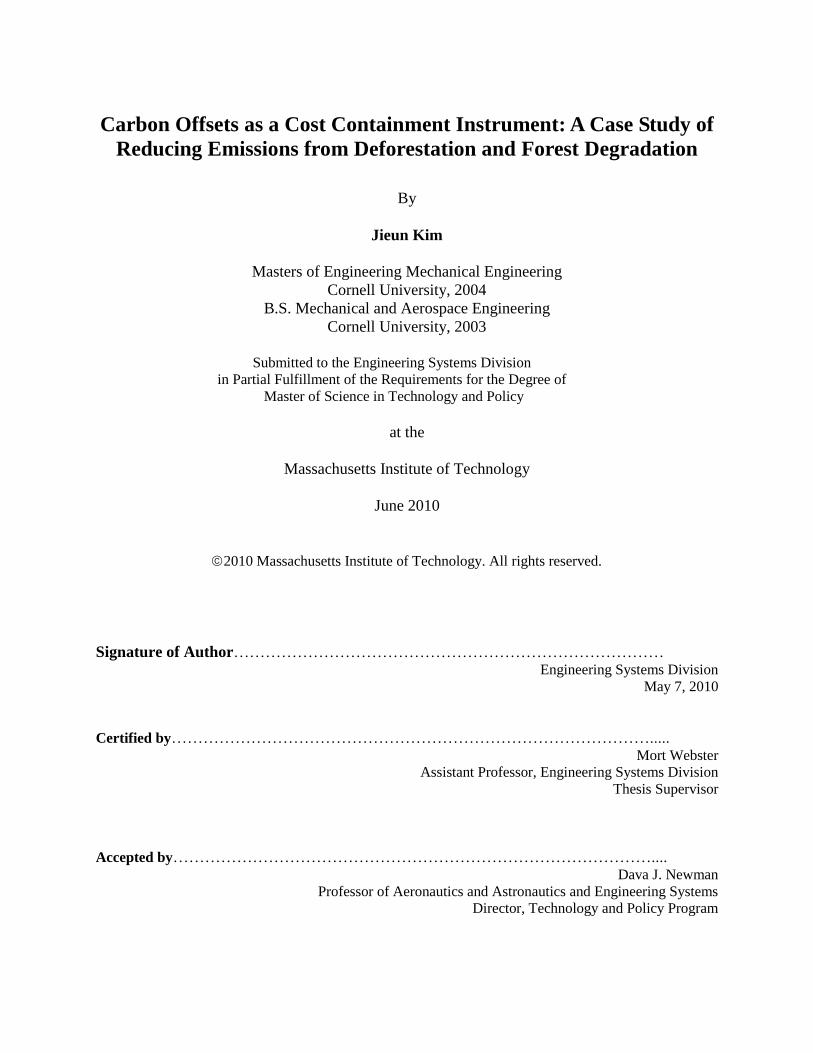
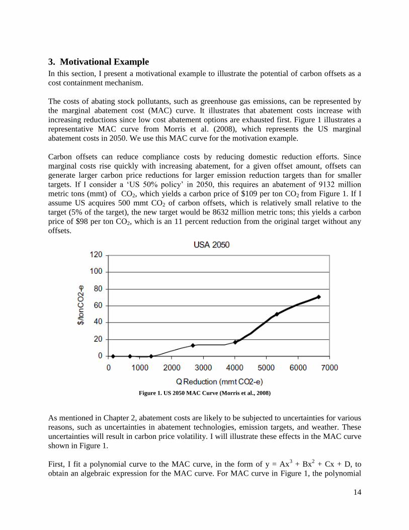
The costs of abating stock pollutants, such as greenhouse gas emissions, can be represented by

the marginal abatement cost (MAC) curve. It illustrates that abatement costs increase with

increasing reductions since low cost abatement options are exhausted first. Figure 1 illustrates a

representative MAC curve from Morris et al. (2008), which represents the US marginal

abatement costs in 2050. We use this MAC curve for the motivation example.

Carbon offsets can reduce compliance costs by reducing domestic reduction efforts. Since

marginal costs rise quickly with increasing abatement, for a given offset amount, offsets can

generate larger carbon price reductions for larger emission reduction targets than for smaller

targets. If I consider a ‗US 50% policy‘ in 2050, this requires an abatement of 9132 million

metric tons (mmt) of CO2, which yields a carbon price of $109 per ton CO2 from Figure 1. If I

assume US acquires 500 mmt CO2 of carbon offsets, which is relatively small relative to the

target (5% of the target), the new target would be 8632 million metric tons; this yields a carbon

price of $98 per ton CO2, which is an 11 percent reduction from the original target without any

offsets.

Figure 1. US 2050 MAC Curve (Morris et al., 2008)

As mentioned in Chapter 2, abatement costs are likely to be subjected to uncertainties for various

reasons, such as uncertainties in abatement technologies, emission targets, and weather. These

uncertainties will result in carbon price volatility. I will illustrate these effects in the MAC curve

shown in Figure 1.

First, I fit a polynomial curve to the MAC curve, in the form of y = Ax3 + Bx

2 + Cx + D, to

obtain an algebraic expression for the MAC curve. For MAC curve in Figure 1, the polynomial

15

fit is: -4E-11x3 + 2E-6x

2 – 0.0031x + 0.9704. This polynomial fit shows that higher order effects

beyond the second-order term may play a diminished role, as shown by the smaller coefficient

value.

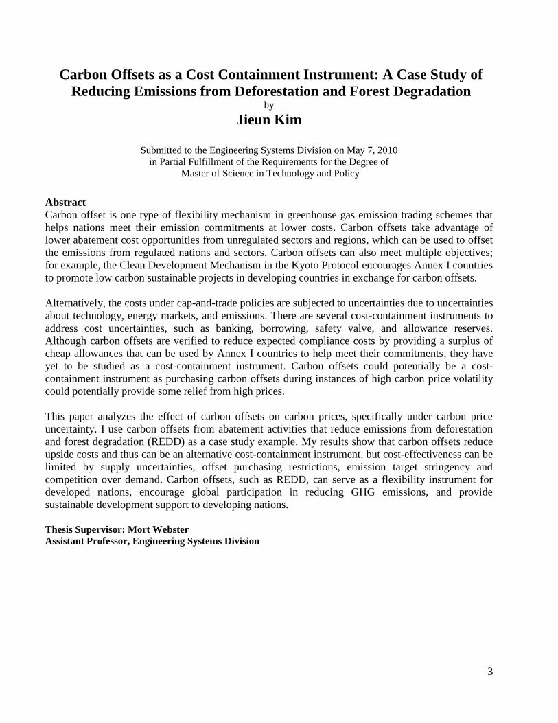
I illustrate uncertainties in carbon prices by imposing a distribution on each polynomial

coefficient (A, B, C, and D). For this example, I replace only one coefficient at a time with a

distribution ranging from half to twice the nominal coefficient value. The same process is

completed for the other coefficients, and I get a distribution of carbon prices as shown in Figure

2 for each coefficient uncertainty.

Figure 2 illustrates the effect of uncertainty on carbon prices. These figures overlay the nominal

MAC curve with MAC at the upper and lower bounds of the imposed coefficient distribution.

With an emissions reduction target of 9132mmt CO2 from above, uncertainties in coefficients A,

B, and C produce high carbon price volatilities. In addition, the effect of the 500mmt CO2 carbon

offset on carbon price varies over the coefficient distribution; this is mostly evident in

‗Uncertainty in B‘ results, the reduction in carbon price is greater in the upper bound than the

lower bound, as shown by the circles in each curve (dark-colored circle represents original target,

light-colored circle represents new target with offsets).

Figure 2. MAC curves with uncertainty bounds

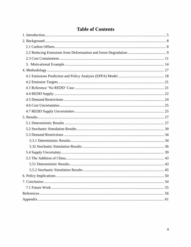
I further examine the role of carbon offsets under MAC uncertainties using Monte Carlo

Analysis. Using the imposed probability distributions on each polynomial coefficient, I extract

10,000 random samples from each coefficient distribution; these samples are used simulate

16

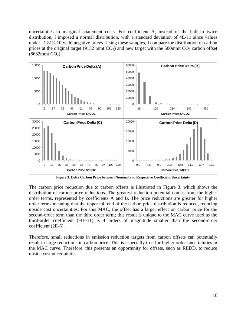
uncertainties in marginal abatement costs. For coefficient A, instead of the half to twice

distribution, I imposed a normal distribution, with a standard deviation of 4E-11 since values

under –1.81E-10 yield negative prices. Using these samples, I compare the distribution of carbon

prices at the original target (9132 mmt CO2) and new target with the 500mmt CO2 carbon offset

(8632mmt CO2).

0

5000

10000

15000

20000

9.0 9.5 9.9 10.4 10.8 11.3 11.7 12.1

Carbon Price, $/tCO2

Carbon Price Delta (D)

0

5000

10000

15000

20000

25000

30000

3 15 26 38 50 62 73 85 97 109 120


Carbon Price Delta (C)

0

10000

20000

30000

40000

50000

60000

18 126 234 342 450


Carbon Price Delta (B)

0

5000

10000

15000

2 17 32 46 61 76 90 105 120


Carbon Price Delta (A)

Figure 3. Delta Carbon Price between Nominal and Respective Coefficient Uncertainty

The carbon price reduction due to carbon offsets is illustrated in Figure 3, which shows the

distribution of carbon price reductions. The greatest reduction potential comes from the higher

order terms, represented by coefficients A and B. The price reductions are greater for higher

order terms meaning that the upper tail end of the carbon price distribution is reduced, reducing

upside cost uncertainties. For this MAC, the offset has a larger effect on carbon price for the

second-order term than the third order term; this result is unique to the MAC curve used as the

third-order coefficient (-4E-11) is 4 orders of magnitude smaller than the second-order

coefficient (2E-6).

Therefore, small reductions in emission reduction targets from carbon offsets can potentially

result in large reductions in carbon price. This is especially true for higher order uncertainties in

the MAC curve. Therefore, this presents an opportunity for offsets, such as REDD, to reduce

upside cost uncertainties.

17

4. Methodology In this chapter, I describe the framework and assumptions used to simulate the effect of REDD

offsets. The analysis requires an assumption about the linked emissions trading schemes into

which offsets would be traded, along with respective regional GHG emission commitments. In

addition, the following REDD details are needed: quantity of REDD available (REDD supply),

and REDD supplying regions with their respective business-as-usual baselines to ensure

additionality.

Moreover, as verified in the EPA study of the Lieberman-Warner bill (EPA, 2008) through

restrictions on domestic and/or international offsets, offset scarcity impacts expected compliance

costs; therefore, offset scarcity could also impact cost-containment. Scarcity is influenced by

changes in the supply of and the demand for offsets. For REDD, supply is the amount of REDD

credits allocated to these high-risk deforestation regions, and demand is the amount of REDD

credits acquired by each region. Therefore, I analyze several limitations on the demand for and

supply of REDD to determine the scarcity effects on cost-containment.

I examine two factors that influence demand: competition (number of buyers) and offset demand

restrictions. Competition increases overall demand for offsets thereby making offsets scarcer for

all offset buyers, as the supply of offsets cannot compensate for the increase in demand. Offset

demand restrictions are limitations on the amount of offsets allowed to enter an emissions trading

scheme. I simulate competition by modeling four trading scenarios, with increasing number of

REDD buyers, to represent low to high competition. In addition, I apply the 1 billion metric ton

CO2 international offset restriction from the Waxman-Markey Bill (H.R. 2454) to simulate US

offset demand restrictions.

There are uncertainties that impact the allocation of offsets in each region, which can be

influenced by a number of factors, such as certification and opportunity costs. I examine supply

uncertainties based on opportunity costs and deployment uncertainties. I generate two alternative

supply probability distributions representing the following two supply scenarios: (1) combined

opportunity and deployment uncertainties, and (2) opportunity cost uncertainties based on fast

deployment. I examine these two supply scenarios via Monte Carlo simulation; using randomly

drawn samples from these two distributions, I analyze the two different supply scenarios with

REDD to determine the effect of supply uncertainties on cost-containment.

I model REDD both deterministically and stochastically. The deterministic results illustrate the

effects of REDD on expected compliance costs under the different trading scenarios and under

US offset demand restrictions. The stochastic analysis assesses REDD offsets on carbon price

and supply uncertainties under the different trading scenarios and US offset demand restrictions.

To model cost uncertainties, I use Monte Carlo simulation with 400 samples that are drawn from

probability distributions for 110 EPPA model parameters that are found to impact emissions and

cost. I simulate the effects of including REDD, under these cost uncertainties, for each of the

different trading scenarios and US offset demand restrictions to determine whether REDD offsets

exhibit cost-containment behavior and whether competition and offset demand restrictions limit

cost-containment effectiveness. The supply uncertainties are assessed similarly to cost

18

uncertainties; I incorporate the samples drawn from the two supply distributions with the cost

uncertainty samples and assess the different trading scenarios and US offset demand restrictions.

I examine four trading scenarios with increasing competition, with the following designated

REDD buyers: (1) US only; (2) Canada, Japan, European Union, Australia, New Zealand added;

(3) China added; (4) All regions. I will refer trading scenario 2 as ‗Annex 1‘ even though it does

not include all Annex 1 countries.

I model the offset restrictions in the proposed American Clean Energy and Security Act of 2009

(H.R. 2454, Waxman-Markey Bill) as the offset demand restriction scenario. The bill has a

provision that limits domestic and international offsets to two billion metric tons (bmt) of CO2 –

one bmt for domestic and the rest for international offsets; this can limit cost containment

effectiveness as it artificially makes offsets scarce within the US.

All scenarios described above are analyzed using a computational general equilibrium (CGE)

model, MIT Emissions Prediction and Policy Analysis (EPPA) Model. The following sections

will discuss the supply and demand assumptions and emission targets in further detail as well as

how they are incorporated in the EPPA model.

4.1 Emissions Prediction and Policy Analysis (EPPA) Model

I use Version 4 of the Emissions Prediction and Policy Analysis (EPPA) model. The EPPA

model is a CGE model developed by the MIT Joint Program on the Science and Policy of Global

Change. The EPPA model is a multi-region, multi-sector recursive-dynamic representation of the

global economy (Paltsev et al., 2005). In a recursive-dynamic solution economic actors are

modeled as having ―myopic‖ expectations.1 This assumption means that current period

investment, savings, and consumption decisions are made on the basis of current period prices.

The EPPA model is built on the GTAP dataset (Hertel, 1997; Dimaranan and McDougall, 2002),

which accommodates a consistent representation of energy markets in physical units as well as

detailed data on regional production, consumption, and bilateral trade flows. Besides the GTAP

dataset, EPPA uses additional data for greenhouse gases and air pollutant emissions based on

United States Environmental Protection Agency inventory data.

The model is calibrated based upon data organized into social accounting matrices (SAM) that

include quantities demanded and trade flows in a base year denominated in both physical and

value terms. A SAM quantifies the inputs and outputs of each sector, which allow for the

calculation of input shares, or the fraction of total sector expenditures represented by each input.

Much of the sector detail in the EPPA model is focused on providing a more accurate

representation of energy production and use as it may change over time or under policies that

would limit greenhouse gas emissions. The base year of the EPPA model is 1997. From 2000 the

model solves recursively at five-year intervals. Sectors are modeled using nested constant

elasticity of substitution (CES) production functions (with Cobb-Douglass or Leontief forms).

The model is solved in the Mathematical Programming System for General Equilibrium

1 The EPPA model can also be solved as a forward looking model (Gurgel et al., 2007). Solved in that manner the

behavior is very similar in terms of abatement and CO2-e prices compared to a recursive solution with the same

model features. However, the solution requires elimination of some of the technological alternatives.

19

(MPSGE) language as a mixed complementarity problem (Mathiesen, 1985; Rutherford, 1995).

The resulting equilibrium in each period must satisfy three inequalities: the zero profit, market

clearance, and income balance conditions (for more information, see Paltsev et al., 2005).

The level of aggregation of the model is presented in Table 1. The model includes representation

of abatement of CO2

and non-CO2 greenhouse gas emissions (CH

4, N

2O, HFCs, PFCs and SF

6)

and the calculations consider both the emissions mitigation that occurs as a byproduct of actions

directed at CO2 and reductions resulting from gas-specific control measures. Targeted control

measures include reductions in the emissions of: CO2 from the combustion of fossil fuels; the

industrial gases that replace CFCs controlled by the Montreal Protocol and produced at

aluminum smelters; CH4 from fossil energy production and use, agriculture, and waste, and N

2O

from fossil fuel combustion, chemical production and improved fertilizer use. More detail on

how abatement costs are represented for these substances is provided in Hyman et al. (2003).

Non-energy activities are aggregated into six sectors, as shown in the table. The energy sector,

which emits several of the non-CO2 gases as well as CO

2, is modeled in more detail. The

synthetic coal gas industry produces a perfect substitute for natural gas. The oil shale industry

produces a perfect substitute for refined oil. All electricity generation technologies produce

perfectly substitutable electricity except for Solar and Wind technology, which is modeled as

producing an imperfect substitute, to reflect intermittent output.

The regional and sectoral disaggregation is also shown in Table 1. There are 16 geographical

regions represented explicitly in the model including major countries (the US, Japan, Canada,

China, India, and Indonesia) and 10 regions that are an aggregations of countries. Each region

includes detail on economic sectors (agriculture, services, industrial and household

transportation, energy intensive industry) and a more elaborated representation of energy sector

technologies.

20

Table 1. EPPA Model Details.

Country or Region† Sectors Factors

Developed Final Demand Sectors Capital

United States (USA) Agriculture Labor

Canada (CAN) Services Crude Oil Resources

Japan (JPN) Energy-Intensive Products Natural Gas Resources

European Union+ (EUR) Other Industries Products Coal Resources

Australia & New Zealand (ANZ) Transportation Shale Oil Resources

Former Soviet Union (FSU) Household Transportation Nuclear Resources

Eastern Europe (EET) Other Household Demand Hydro Resources

Developing Energy Supply & Conversion Wind/Solar Resources

India (IND) Electric Generation Land

China (CHN) Conventional Fossil

Indonesia (IDZ) Hydro

Higher Income East Asia (ASI) Nuclear

Mexico (MEX) Wind, Solar

Central & South America (LAM) Biomass

Middle East (MES) Advanced Gas (NGCC)

Africa (AFR) Advanced Gas with CCS

Rest of World (ROW) Advanced Coal with CCS

Fuels

Coal

Crude Oil, Shale Oil, Refined Oil

Natural Gas, Gas from Coal

Liquids from Biomass

Synthetic Gas †

Specific detail on regional groupings is provided in Paltsev et al. (2005).

When emissions constraints on certain countries, gases, or sectors are imposed in a CGE model

such as EPPA, the model calculates a shadow value of the constraint which can be interpreted as

a price that would be obtained under an allowance market that developed under a cap and trade

system. Those prices are the marginal costs used in the construction of marginal abatement cost

(MAC) curves. They are plotted against a corresponding amount of abatement, which is the

difference in emissions levels between a no policy reference case and a policy-constrained case.

The solution algorithm of the EPPA model finds least-cost reductions for each gas in each sector

and if emissions trading is allowed it equilibrates the prices among sectors and gases (using

GWP weights). This set of conditions, often referred to as ―what‖ and ―where‖ flexibility, will

tend to lead to least-cost abatement. Without these conditions abatement costs will vary among

sources and that will affect the estimated welfare cost—abatement will be least-cost within a

sector or region or for a specific gas, but will not be equilibrated among them.

The results depend on a number of aspects of model structure and particular input assumptions

that greatly simplify the representation of economic structure and decision-making. For

example, the difficulty of achieving any emissions path is influenced by assumptions about

21

population and productivity growth that underlie the no-policy reference case. The simulations

also embody a particular representation of the structure of the economy, including the relative

ease of substitution among the inputs to production and the behavior of consumers in the face of

changing prices of fuels, electricity and other goods and services. Further critical assumptions

must be made about the cost and performance of new technologies and what might limit their

market penetration. Alternatives to conventional technologies in the electric sector and in

transportation are particularly significant. Finally, the EPPA model draws heavily on

neoclassical economic theory. While this underpinning is a strength in some regards, the model

fails to capture economic rigidities that could lead to unemployment or misallocation of

resources nor does it capture regulatory and policy details that can be important in regulated

sectors such as power generation.

I use EPPA to compare shadow prices (i.e., carbon prices) with and without REDD under

emission constraints and different trading scenarios.

4.2 Emission Targets

The compliance period for the Kyoto Protocol commitments is 2008 through 2012. Since REDD

market entry is not foreseeable during the Kyoto Protocol compliance period, I assume that

REDD credits will be available as part of an emission trading scheme under a post-Kyoto

agreement. To model REDD, this requires assuming hypothetical emission commitments for all

participating regions as targets are not finalized. Based on the 2009 G8 Summit talks and

CLEAR (Carbon Limits + Early Action = Rewards) Target (Wagner et al., 2009), I assume the

following targets.

US

OECD

Europe Russia

Canada, Japan, Rest

of OECD Pacific

Rest of E.

Europe/Eurasia Developing Countries

2020 -17% -20% -10% 10% -10% BAU until 2018

2050 -80% -80% -80% -80% -50% -30% * % difference from 1990 levels

Conceptually, CLEAR targets, also known as Clean Investment Budgets, represent the idea that

emerging economies adopt targets that are initially above current levels but within the 2 degree

Celsius global goal2; this provides immediate availability of allowances for industrialized nations

while providing funding for emerging economies to transition to a low-carbon economy (Wagner

et al., 2009). In the 2009 G8 Summit in L‘Aquila Italy, G8 countries have committed to reduce

their GHG emissions by 80% by 2050 from 1990 levels, and other major emitting countries have

agreed to reduce their emissions by 50% by 2050 (G8 Summit Papers, 2009). For developing

countries, I modeled a stringent scenario where they reach a 30 percent reduction below their

respective 1990 levels by 2050, with reductions starting in 2019. These developing countries

include the REDD supplying regions. All emission targets are assumed to decline linearly.

4.3 Reference ‘No REDD’ Case

Emissions trading allow participating nations to reduce emissions cost-effectively. In addition,

carbon offsets come in many forms. Therefore, the effects of REDD trading needs to be isolated

2 Agreement to keep mean global temperature within 2 degrees Celsius above pre-industrial level

22

from non-REDD offsets (i.e., trading emissions reductions in industrial sectors) to understand the

sole effect of REDD credits. I designate the trading scenario without REDD as the reference ‗No

REDD‘ case, which is modeled as the emissions targets described above with full global

emissions trading allowed. The REDD allowances are then added to the resulting emissions from

the ‗No REDD‘ case, and these new emissions are imposed as the new emission caps. This

allows REDD offsets to be isolated from other allowances and other non-REDD offsets.

Therefore, REDD trading occurs ex post the reference case, where all other offset and

allowances are traded prior to REDD entering the market. These revised emission targets are

added as a constraint in EPPA and are used for all scenarios for comparison purposes.

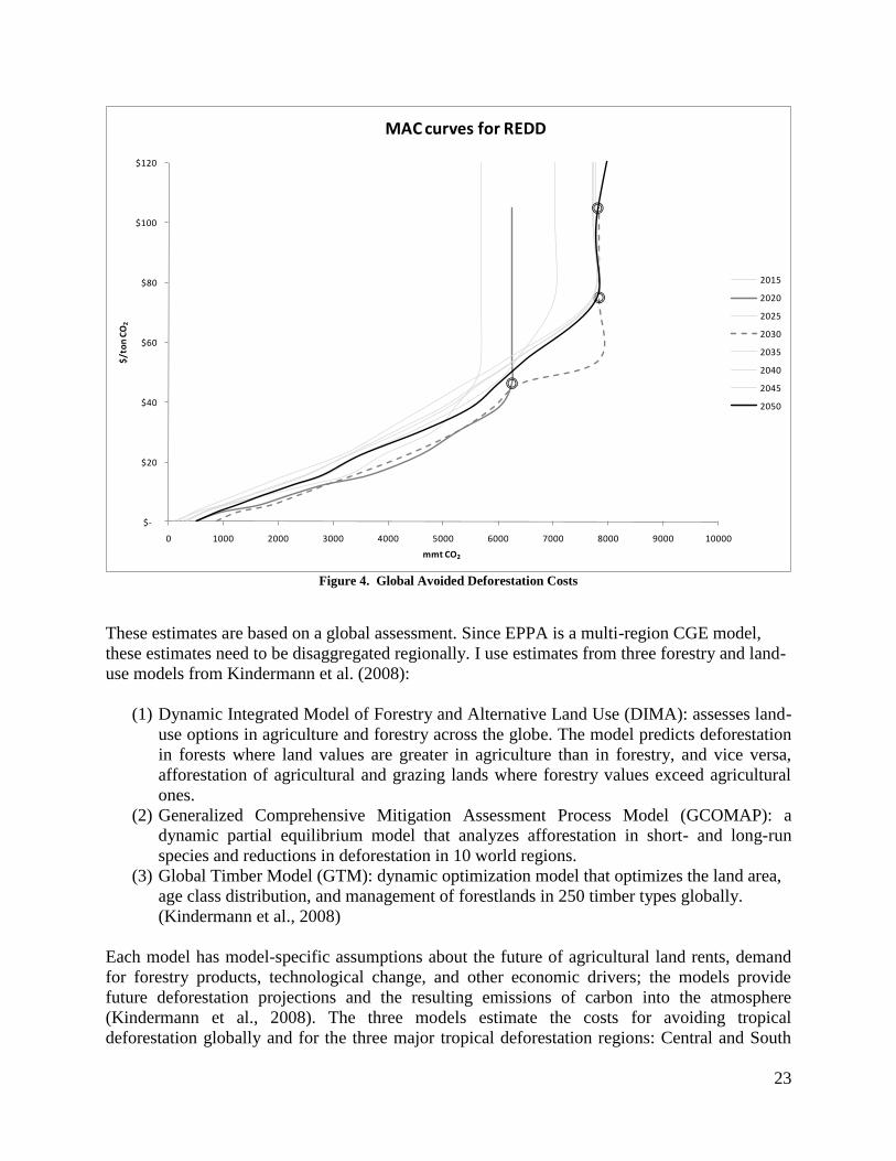
4.4 REDD Supply

I use marginal cost estimates to capture the potential supply of REDD. The marginal cost curves

relate the opportunity costs of REDD to the amount of emissions reduced from REDD-activities;

these costs include the forgone profits from reduced deforestation in sectors such as agricultural,

or forestry products, as well as administrative costs to cover forest management.

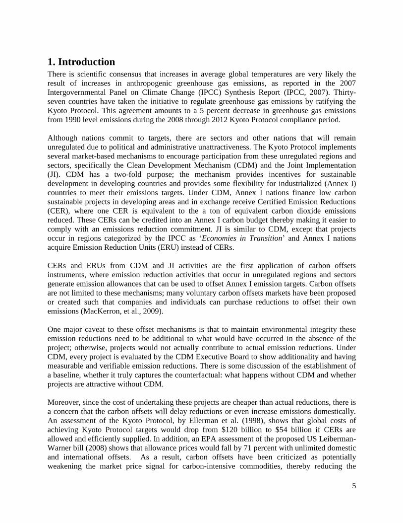
I use an amended MAC curve based on estimates from the Global Timber Model (GTM). The

Global Timber Model3 is a partial equilibrium intertemporal optimization economic model that

maximizes welfare across 250 world timber supply regions through the management of forest

stand ages, compositions, and acreage given production and land rental costs. The model

simulates trade responses to policy by predicting supply responses to current and future prices

(EPA Analysis of H.R. 2454, 2010). The model assumes that all international mitigation

practices are eligible from 2010 to 2050, and that mitigation activity is disaggregated into

afforestation, forest management, and avoided deforestation. The model estimates the aggregated

international forestry marginal abatement costs (EPA Analysis of H.R. 2454, 2010). Using

estimated shares of total forest carbon mitigation attributed to reduced deforestation from Murray

et al. (2009), the MAC is adjusted to reflect mitigation from reduced deforestation activities

(Figure 4).

Typically we would just equate the REDD supply and regional MAC curves to determine the

cost-effective allocation of REDD. However, REDD is not implemented endogenously in EPPA

and cannot represent REDD MAC curves explicitly. I allocate a fixed supply of REDD

allowances over time, based on the MAC curve in Figure 4. For the base case, I use the

maximum available REDD in each year, which I define as the level at which costs turn vertical -

as noted by the circles in Figure 4.

3 Developed by Brent Sohngen from the Department of Agricultural, Environmental, and Developmental Economics

(Ohio State University) with collaboration from Robert Mendlesohn, Roger Sedjo, and Kenneth Lyon

23

$-

$20

$40

$60

$80

$100

$120

0 1000 2000 3000 4000 5000 6000 7000 8000 9000 10000

$/t

on

CO

2

mmt CO2

MAC curves for REDD

2015

2020

2025

2030

2035

2040

2045

2050

Figure 4. Global Avoided Deforestation Costs

These estimates are based on a global assessment. Since EPPA is a multi-region CGE model,

these estimates need to be disaggregated regionally. I use estimates from three forestry and land-

use models from Kindermann et al. (2008):

(1) Dynamic Integrated Model of Forestry and Alternative Land Use (DIMA): assesses land-

use options in agriculture and forestry across the globe. The model predicts deforestation

in forests where land values are greater in agriculture than in forestry, and vice versa,

afforestation of agricultural and grazing lands where forestry values exceed agricultural

ones.

(2) Generalized Comprehensive Mitigation Assessment Process Model (GCOMAP): a

dynamic partial equilibrium model that analyzes afforestation in short- and long-run

species and reductions in deforestation in 10 world regions.

(3) Global Timber Model (GTM): dynamic optimization model that optimizes the land area,

age class distribution, and management of forestlands in 250 timber types globally.

(Kindermann et al., 2008)

Each model has model-specific assumptions about the future of agricultural land rents, demand

for forestry products, technological change, and other economic drivers; the models provide

future deforestation projections and the resulting emissions of carbon into the atmosphere

(Kindermann et al., 2008). The three models estimate the costs for avoiding tropical

deforestation globally and for the three major tropical deforestation regions: Central and South

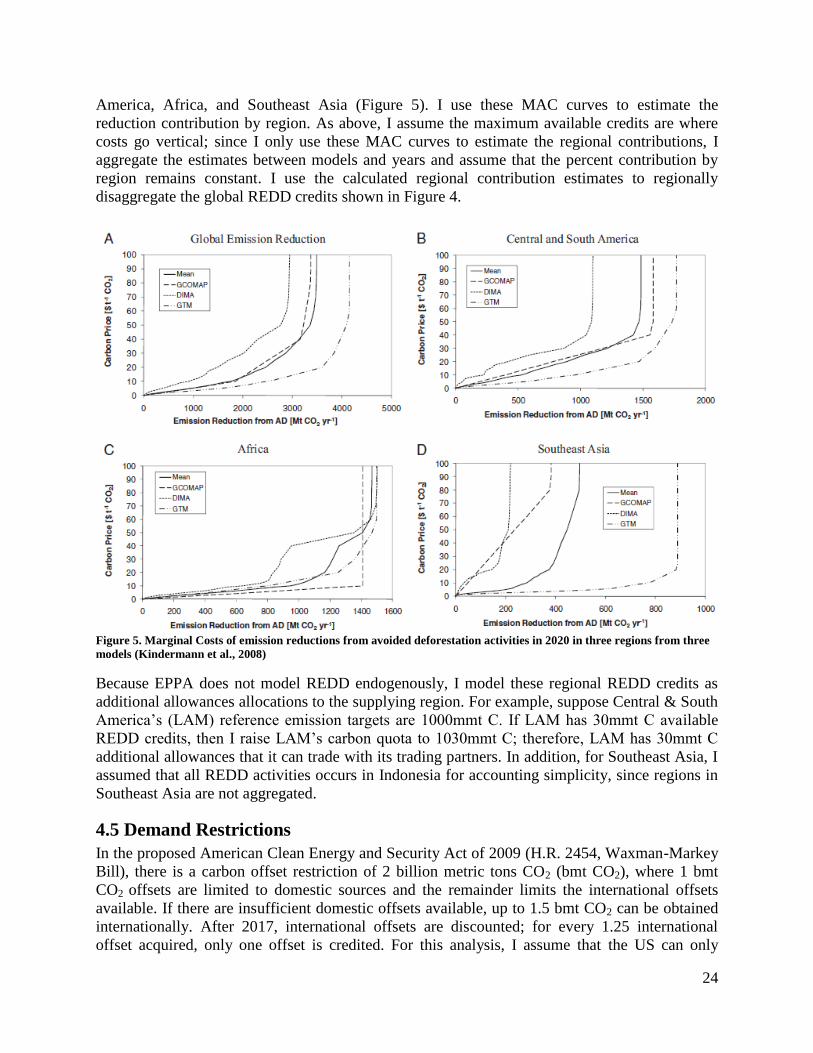
24

America, Africa, and Southeast Asia (Figure 5). I use these MAC curves to estimate the

reduction contribution by region. As above, I assume the maximum available credits are where

costs go vertical; since I only use these MAC curves to estimate the regional contributions, I

aggregate the estimates between models and years and assume that the percent contribution by

region remains constant. I use the calculated regional contribution estimates to regionally

disaggregate the global REDD credits shown in Figure 4.

Figure 5. Marginal Costs of emission reductions from avoided deforestation activities in 2020 in three regions from three

models (Kindermann et al., 2008)

Because EPPA does not model REDD endogenously, I model these regional REDD credits as

additional allowances allocations to the supplying region. For example, suppose Central & South

America‘s (LAM) reference emission targets are 1000mmt C. If LAM has 30mmt C available

REDD credits, then I raise LAM‘s carbon quota to 1030mmt C; therefore, LAM has 30mmt C

additional allowances that it can trade with its trading partners. In addition, for Southeast Asia, I

assumed that all REDD activities occurs in Indonesia for accounting simplicity, since regions in

Southeast Asia are not aggregated.

4.5 Demand Restrictions

In the proposed American Clean Energy and Security Act of 2009 (H.R. 2454, Waxman-Markey

Bill), there is a carbon offset restriction of 2 billion metric tons CO2 (bmt CO2), where 1 bmt

CO2 offsets are limited to domestic sources and the remainder limits the international offsets

available. If there are insufficient domestic offsets available, up to 1.5 bmt CO2 can be obtained

internationally. After 2017, international offsets are discounted; for every 1.25 international

offset acquired, only one offset is credited. For this analysis, I assume that the US can only

25

acquire 1bmt CO2 of REDD offsets for all years for my analysis. I only focus on demand

restrictions from the US due to computational limitations.

Since REDD is modeled as additional emission allowance and is available for all trading

partners, the allocation of REDD is the only exogenous constraint on the quantity of REDD

acquired by the US. Therefore, to model the US 1bmt CO2 international offset restriction, I

implemented and iterative-algorithm (in Matlab) to determine the correct REDD allocation such

that US acquires 1bmt CO2 REDD offsets. The methodology is as follows:

1. Start with an initial guess for the starting REDD allocation

2. Call EPPA to run the scenario of interest with the starting REDD allocation.

3. Compare US emissions levels from EPPA to US emissions with 1bmt CO2 REDD offsets

(US reference case emissions + 1bmt CO2)

4. If they diverge, recalculate a new REDD allocation to input into EPPA

5. Repeat until convergence in step 4

Convergence is defined to be where emissions are within 3E-5 of each other.

A limitation of using this approach to model demand constraints is that additional demand

constraints from other regions over-constrains the problem thus making solution is

indeterminate. Therefore, I only focus on US demand restrictions for this study. Since this

method is computationally intensive, I only investigated the two extreme trading scenarios: US-

only and All Regions.

4.6 Cost Uncertainties

To observe cost-containment behavior, cost uncertainties need to be simulated. I apply

assumptions from Webster et al. (2008b), which identified 110 parameters in the EPPA model

that affect emissions growth and abatement costs. These include parameters representing labor

productivity growth rates, energy efficiency trends, elasticities of substitution, cost of advanced

technologies, fossil fuel resource availability, and urban pollutant trends (Webster et al., 2008b).

Probability distributions for these parameters were developed based on historical data and expert

judgment.

Here, I perform Monte Carlo simulation using Latin Hypercube sampling with 400 samples

drawn from each of the parameter distributions. These samples are input into the EPPA model to

generate cost uncertainties. I compare the carbon prices with and without REDD under different

trading scenarios and US offset restrictions to determine if REDD exhibits cost containing

behavior and if trading scenarios and offset demand restriction limit cost-containing behavior.

4.7 REDD Supply Uncertainties

There are underlying uncertainties in the REDD supply estimates, primarily from uncertainties in

opportunity costs estimates and deployment estimates. Since opportunity costs consist of forgone

profits from deforestation-related activities, they are influenced by agricultural prices and other

market prices, which, like all markets, are subjected to uncertainties. In addition, deployment of

these credits depends on a country‘s readiness level to enter the market, which can be due to

access to monitoring and operating forest management system. While there are efforts from the

26

Bali Action Plan to encourage REDD-readiness activities, there is no certainty as to how much

REDD will actually be available in the emissions trading scheme.

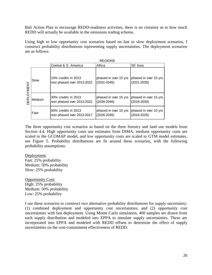
Using high to low opportunity cost scenarios based on fast to slow deployment scenarios, I

construct probability distributions representing supply uncertainties. The deployment scenarios

are as follows:

Central & S. America Africa SE Asia

Slow10% credits in 2013

rest phased over 2013-2022

phased in over 15 yrs

(2031-2045)


(2021-2035)

Medium30% credits in 2013



(2026-2040)


(2016-2030)

Fast50% credits in 2013



(2026-2035)


(2016-2025)

REGIONS

DE

PLO

YM

EN

T

The three opportunity cost scenarios as based on the three forestry and land use models from

Section 4.4. High opportunity costs use estimates from DIMA; medium opportunity costs are

scaled to the GCOMAP model, and low opportunity costs are scaled to GTM model estimates,

see Figure 5. Probability distributions are fit around these scenarios, with the following

probability assumptions:

Deployment:

Fast: 25% probability

Medium: 50% probability

Slow: 25% probability

Opportunity Cost:

High: 25% probability

Medium: 50% probability

Low: 25% probability

I use these scenarios to construct two alternative probability distributions for supply uncertainty:

(1) combined deployment and opportunity cost uncertainties; and (2) opportunity cost

uncertainties with fast deployment. Using Monte Carlo simulation, 400 samples are drawn from

each supply distribution and modeled into EPPA to simulate supply uncertainties. These are

incorporated into EPPA and modeled with REDD offsets to determine the effect of supply

uncertainties on the cost-containment effectiveness of REDD.

27

5. Results I analyzed REDD offsets deterministically and stochastically. The deterministic results illustrate

the effect of REDD offsets on expected costs. The stochastic analysis assesses the effects of

REDD on carbon price uncertainty, which is the central to understand whether REDD reduces

upside risk through cost-containment. As mentioned in Chapter 4, I analyze two demand and

supply scenarios to assess the effect of increased scarcity of REDD on carbon price. The demand

scenarios examine the effect of (1) competition over demand for REDD as seen by increasing the

number of regions that can purchase REDD, and (2) limitations on the number of REDD credits

a region can purchase. Supply scenarios are based on opportunity cost uncertainties of REDD

based on a range of deployment rates.

In Section 5.1, I present the results of the deterministic scenario analysis. Section 5.2 presents

Monte Carlo results of REDD without supply uncertainties, both Section 5.1 and 5.2 assume no

restriction on offset purchases. Section 5.3 presents the results of the US restriction on offsets

purchases using deterministic and Monte Carlo analysis. Section 5.4 presents Monte Carlo

results with supply uncertainties. Lastly, Section 5.5 presents the results of the special scenario

where China is allowed to purchase REDD offsets with Annex I regions; this scenario is

analyzed both deterministically and stochastically.

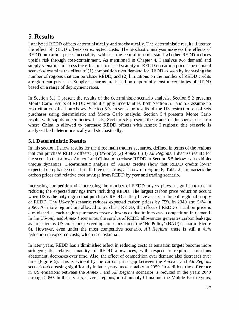
5.1 Deterministic Results

In this section, I show results for the three main trading scenarios, defined in terms of the regions

that can purchase REDD offsets: (1) US-only; (2) Annex I; (3) All Regions. I discuss results for

the scenario that allows Annex I and China to purchase REDD in Section 5.5 below as it exhibits

unique dynamics. Deterministic analysis of REDD credits show that REDD credits lower

expected compliance costs for all three scenarios, as shown in Figure 6; Table 2 summarizes the

carbon prices and relative cost savings from REDD by year and trading scenario.

Increasing competition via increasing the number of REDD buyers plays a significant role in

reducing the expected savings from including REDD. The largest carbon price reduction occurs

when US is the only region that purchases REDD as they have access to the entire global supply

of REDD. The US-only scenario reduces expected carbon prices by 75% in 2040 and 54% in

2050. As more regions are allowed to purchase REDD, the effect of REDD on carbon price is

diminished as each region purchases fewer allowances due to increased competition in demand.

In the US-only and Annex I scenarios, the surplus of REDD allowances generates carbon leakage,

as indicated by US emissions exceeding emissions under the ‗No Policy‘ (BAU) scenario (Figure

6). However, even under the most competitive scenario, All Regions, there is still a 41%

reduction in expected costs, which is substantial.

In later years, REDD has a diminished effect in reducing costs as emission targets become more

stringent; the relative quantity of REDD allowances, with respect to required emissions

abatement, decreases over time. Also, the effect of competition over demand also decreases over

time (Figure 6). This is evident by the carbon price gap between the Annex I and All Regions

scenarios decreasing significantly in later years, most notably in 2050. In addition, the difference

in US emissions between the Annex I and All Regions scenarios is reduced in the years 2040

through 2050. In these years, several regions, most notably China and the Middle East regions,

28

purchase fewer REDD offsets under the All Regions scenario thus allowing the US and other

Annex I nations to purchase more REDD thereby reducing the difference in emissions in Annex

I regions for the Annex I and All Regions scenarios, as observed in US emissions in Figure 6.

These trading dynamics generate more cost savings for the All Regions scenario for 2040 through

2050 thus reducing the carbon price difference between Annex I and All Regions.

Table 2. Carbon Prices for different trading scenarios and percent reduction from 'No REDD' Reference Case

29

Figure 6. US Emissions and Carbon Prices under three REDD Trading Scenarios

30

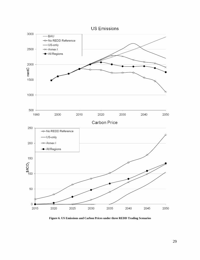
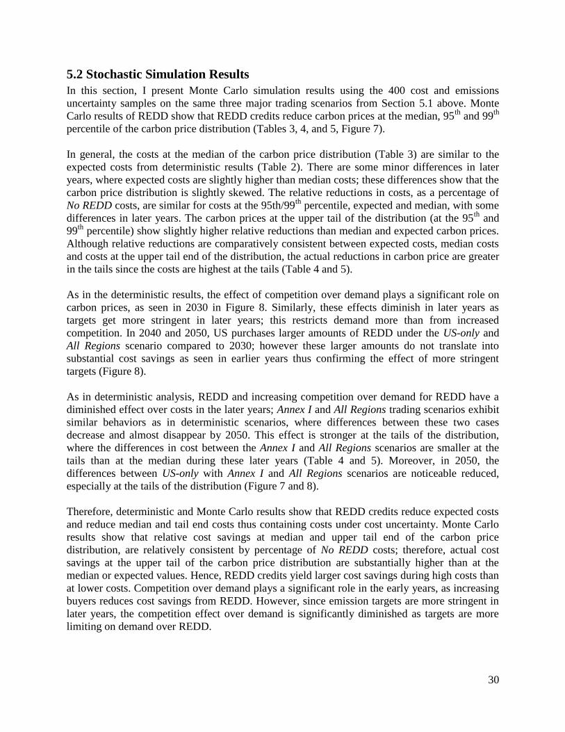
5.2 Stochastic Simulation Results

In this section, I present Monte Carlo simulation results using the 400 cost and emissions

uncertainty samples on the same three major trading scenarios from Section 5.1 above. Monte

Carlo results of REDD show that REDD credits reduce carbon prices at the median, 95th

and 99th

percentile of the carbon price distribution (Tables 3, 4, and 5, Figure 7).

In general, the costs at the median of the carbon price distribution (Table 3) are similar to the

expected costs from deterministic results (Table 2). There are some minor differences in later

years, where expected costs are slightly higher than median costs; these differences show that the

carbon price distribution is slightly skewed. The relative reductions in costs, as a percentage of

No REDD costs, are similar for costs at the 95th/99th

percentile, expected and median, with some

differences in later years. The carbon prices at the upper tail of the distribution (at the 95th

and

99th

percentile) show slightly higher relative reductions than median and expected carbon prices.

Although relative reductions are comparatively consistent between expected costs, median costs

and costs at the upper tail end of the distribution, the actual reductions in carbon price are greater

in the tails since the costs are highest at the tails (Table 4 and 5).

As in the deterministic results, the effect of competition over demand plays a significant role on

carbon prices, as seen in 2030 in Figure 8. Similarly, these effects diminish in later years as

targets get more stringent in later years; this restricts demand more than from increased

competition. In 2040 and 2050, US purchases larger amounts of REDD under the US-only and

All Regions scenario compared to 2030; however these larger amounts do not translate into

substantial cost savings as seen in earlier years thus confirming the effect of more stringent

targets (Figure 8).

As in deterministic analysis, REDD and increasing competition over demand for REDD have a

diminished effect over costs in the later years; Annex I and All Regions trading scenarios exhibit

similar behaviors as in deterministic scenarios, where differences between these two cases

decrease and almost disappear by 2050. This effect is stronger at the tails of the distribution,

where the differences in cost between the Annex I and All Regions scenarios are smaller at the

tails than at the median during these later years (Table 4 and 5). Moreover, in 2050, the

differences between US-only with Annex I and All Regions scenarios are noticeable reduced,

especially at the tails of the distribution (Figure 7 and 8).

Therefore, deterministic and Monte Carlo results show that REDD credits reduce expected costs

and reduce median and tail end costs thus containing costs under cost uncertainty. Monte Carlo

results show that relative cost savings at median and upper tail end of the carbon price

distribution, are relatively consistent by percentage of No REDD costs; therefore, actual cost

savings at the upper tail of the carbon price distribution are substantially higher than at the

median or expected values. Hence, REDD credits yield larger cost savings during high costs than

at lower costs. Competition over demand plays a significant role in the early years, as increasing

buyers reduces cost savings from REDD. However, since emission targets are more stringent in

later years, the competition effect over demand is significantly diminished as targets are more

limiting on demand over REDD.

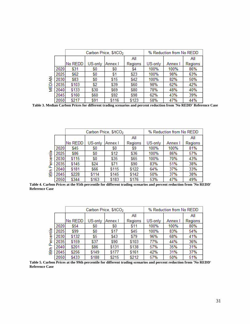
31

Table 3. Median Carbon Prices for different trading scenarios and percent reduction from 'No REDD' Reference Case

Table 4. Carbon Prices at the 95th percentile for different trading scenarios and percent reduction from 'No REDD'

Reference Case

Table 5. Carbon Prices at the 99th percentile for different trading scenarios and percent reduction from 'No REDD'

Reference Case

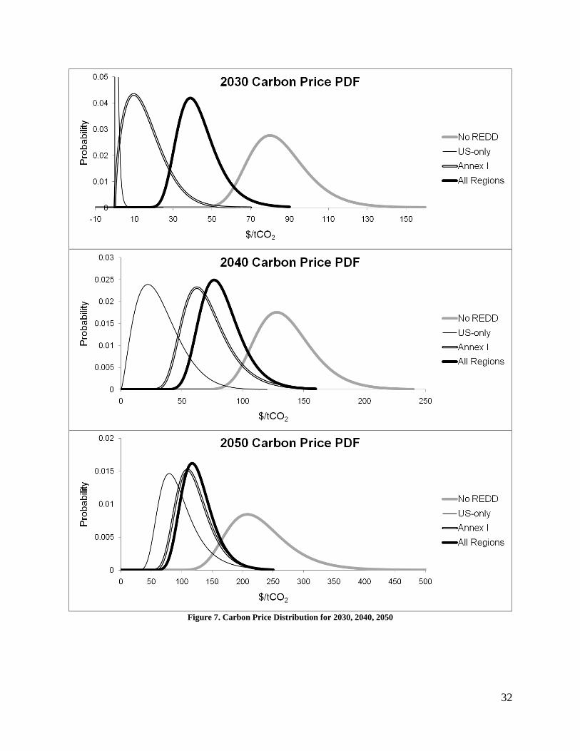
32

Figure 7. Carbon Price Distribution for 2030, 2040, 2050

33

Figure 8. Carbon Price vs. Median REDD Acquired by US in 2030, 2040, and 2050

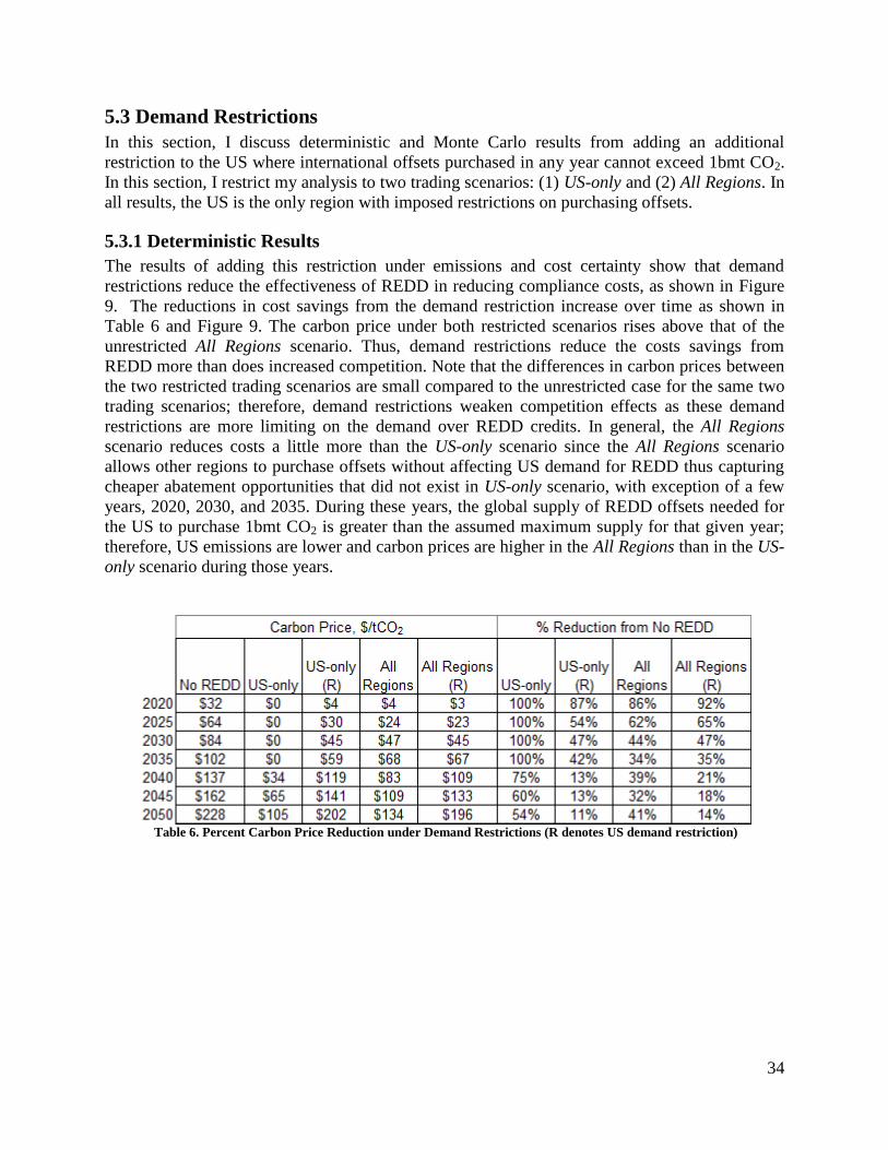
34

5.3 Demand Restrictions

In this section, I discuss deterministic and Monte Carlo results from adding an additional

restriction to the US where international offsets purchased in any year cannot exceed 1bmt CO2.

In this section, I restrict my analysis to two trading scenarios: (1) US-only and (2) All Regions. In

all results, the US is the only region with imposed restrictions on purchasing offsets.

5.3.1 Deterministic Results

The results of adding this restriction under emissions and cost certainty show that demand

restrictions reduce the effectiveness of REDD in reducing compliance costs, as shown in Figure

9. The reductions in cost savings from the demand restriction increase over time as shown in

Table 6 and Figure 9. The carbon price under both restricted scenarios rises above that of the

unrestricted All Regions scenario. Thus, demand restrictions reduce the costs savings from

REDD more than does increased competition. Note that the differences in carbon prices between

the two restricted trading scenarios are small compared to the unrestricted case for the same two

trading scenarios; therefore, demand restrictions weaken competition effects as these demand

restrictions are more limiting on the demand over REDD credits. In general, the All Regions

scenario reduces costs a little more than the US-only scenario since the All Regions scenario

allows other regions to purchase offsets without affecting US demand for REDD thus capturing

cheaper abatement opportunities that did not exist in US-only scenario, with exception of a few

years, 2020, 2030, and 2035. During these years, the global supply of REDD offsets needed for

the US to purchase 1bmt CO2 is greater than the assumed maximum supply for that given year;

therefore, US emissions are lower and carbon prices are higher in the All Regions than in the US-

only scenario during those years.

Table 6. Percent Carbon Price Reduction under Demand Restrictions (R denotes US demand restriction)

35

Figure 9. US Emissions and Carbon Price under US Demand Restrictions (Deterministic)

36

5.32 Stochastic Simulation Results

As in the deterministic results, US demand restrictions significantly reduce the cost savings from

REDD for all years. Carbon price distributions for the restricted US-only scenario start

overlapping the distribution from the unrestricted All Regions scenario in early years and shifts

further right (towards increasing carbon price) (Figure 10). As in deterministic results, costs

under both restricted US-only and restricted All Regions scenario are higher than costs under the

unrestricted All Regions scenario at the median and at the tails of the carbon price distribution

(Tables 7, 8, and 9).

In general, the US offset restriction slightly skews the carbon price distribution slightly to the

right, except for 2040. This effect is more pronounced for the restricted US-only scenario. The

restricted All Regions scenario shows no skew for 2035 and 2040. Similar to deterministic

results, the restricted All Regions scenario generally has lower costs than the restricted US-only

scenario.

Note that even though we establish a ‗No REDD‘ reference, the trade of additional non-REDD

offsets is unavoidable based on the current exogenous implementation of offsets in EPA.

Therefore, there are residual non-REDD (i.e., industrial emission reduction) allowances traded,

but these remain small compared to REDD. However, this effect is pronounced for the restricted

scenarios at the 99th

percentile for 2045 and 2050, where costs exceed the No REDD case. For

the restricted US-only scenario, during these last years, extreme high costs at the tail end cause

REDD supplying regions, especially Central and South America and Africa, to trade non-REDD

offsets, in addition to REDD offsets; as a result, emissions to drop below No REDD reference

emissions for these REDD supplying regions thus raising costs for these later years. Moreover,

during these years, the costs from restricted All Regions scenario exceed the costs from the

restricted US-only scenario at the upper tail end of the distribution thereby further exceeding No

REDD costs. These higher costs at the tail end of the distribution for the restricted All Regions

scenario is a result of emission trading dynamics; some regions, particularly Europe, the Former

Soviet Union, Japan and China, take on significant emission reductions compared to the

restricted US-only scenario. Since most of these regions tend to have high marginal abatement

costs, these emission reductions drive carbon prices higher for the restricted All Regions

scenario.

Therefore, REDD demand restrictions may provide some relief for price shocks for early years;

however, cost savings are substantially reduced even exceeding the most competitive trading

scenario, All Regions, under the case of no purchasing restrictions. In later years, 2045-2050,

these restrictions can effectively render REDD ineffective at reducing carbon price uncertainty.

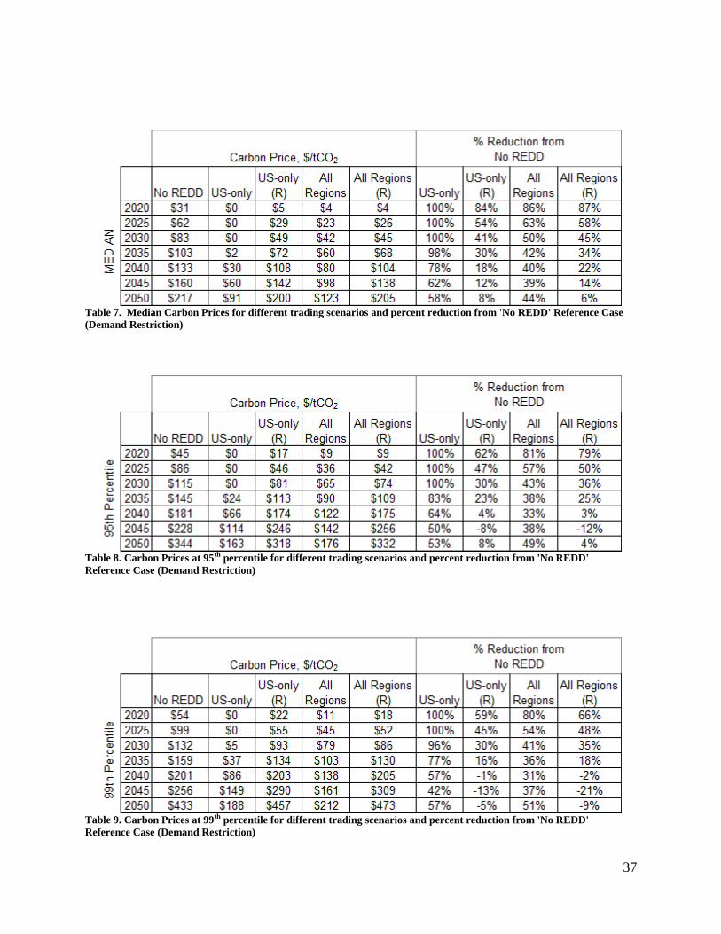
37


(Demand Restriction)

Table 8. Carbon Prices at 95th percentile for different trading scenarios and percent reduction from 'No REDD'

Reference Case (Demand Restriction)


Reference Case (Demand Restriction)

38

Figure 10. Carbon Price Distribution under US Demand Restrictions for 2030, 2040, 2050

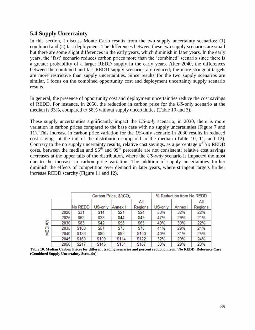
39

5.4 Supply Uncertainty

In this section, I discuss Monte Carlo results from the two supply uncertainty scenarios: (1)

combined and (2) fast deployment. The differences between these two supply scenarios are small

but there are some slight differences in the early years, which diminish in later years. In the early

years, the ‗fast‘ scenario reduces carbon prices more than the ‗combined‘ scenario since there is

a greater probability of a larger REDD supply in the early years. After 2040, the differences

between the combined and fast REDD supply scenarios are reduced; the more stringent targets

are more restrictive than supply uncertainties. Since results for the two supply scenarios are

similar, I focus on the combined opportunity cost and deployment uncertainty supply scenario

results.

In general, the presence of opportunity cost and deployment uncertainties reduce the cost savings

of REDD. For instance, in 2050, the reduction in carbon price for the US-only scenario at the

median is 33%, compared to 58% without supply uncertainties (Table 10 and 3).

These supply uncertainties significantly impact the US-only scenario; in 2030, there is more

variation in carbon prices compared to the base case with no supply uncertainties (Figure 7 and

11). This increase in carbon price variation for the US-only scenario in 2030 results in reduced

cost savings at the tail of the distribution compared to the median (Table 10, 11, and 12).

Contrary to the no supply uncertainty results, relative cost savings, as a percentage of No REDD

costs, between the median and 95th

and 99th

percentile are not consistent; relative cost savings

decreases at the upper tails of the distribution, where the US-only scenario is impacted the most

due to the increase in carbon price variation. The addition of supply uncertainties further

diminish the effects of competition over demand in later years, where stringent targets further

increase REDD scarcity (Figure 11 and 12).


(Combined Supply Uncertainty Scenario)

40


Reference Case (Combined Supply Uncertainty Scenario)


Reference Case (Combined Supply Uncertainty Scenario)

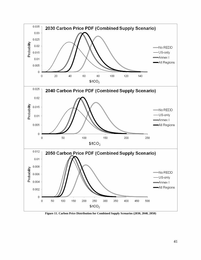
41

Figure 11. Carbon Price Distribution for Combined Supply Scenarios (2030, 2040, 2050)

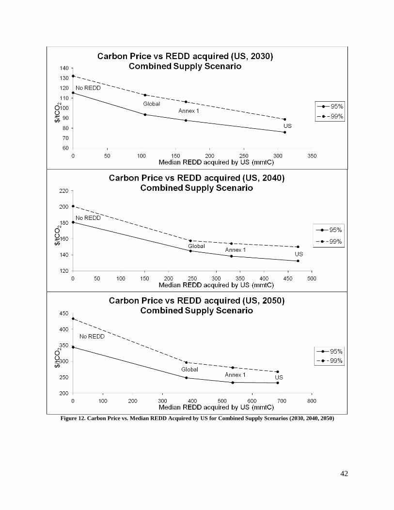
42

Figure 12. Carbon Price vs. Median REDD Acquired by US for Combined Supply Scenarios (2030, 2040, 2050)

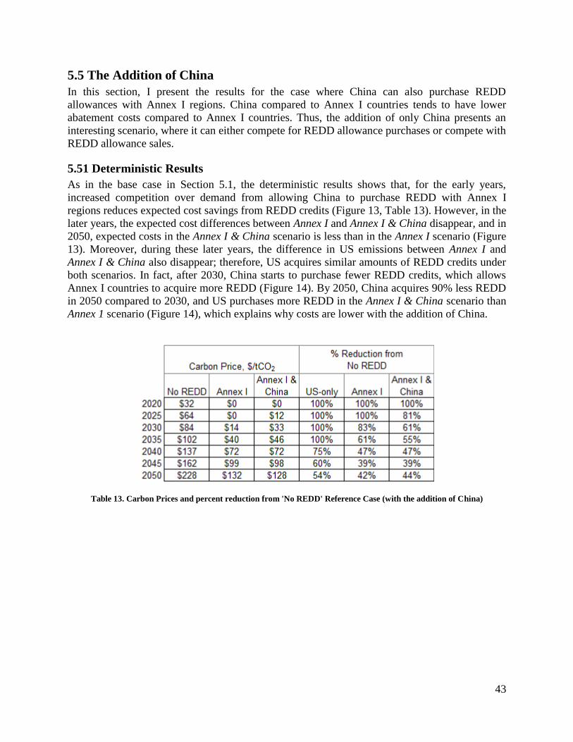
43

5.5 The Addition of China

In this section, I present the results for the case where China can also purchase REDD

allowances with Annex I regions. China compared to Annex I countries tends to have lower

abatement costs compared to Annex I countries. Thus, the addition of only China presents an

interesting scenario, where it can either compete for REDD allowance purchases or compete with

REDD allowance sales.

5.51 Deterministic Results

As in the base case in Section 5.1, the deterministic results shows that, for the early years,

increased competition over demand from allowing China to purchase REDD with Annex I

regions reduces expected cost savings from REDD credits (Figure 13, Table 13). However, in the

later years, the expected cost differences between Annex I and Annex I & China disappear, and in

2050, expected costs in the Annex I & China scenario is less than in the Annex I scenario (Figure

13). Moreover, during these later years, the difference in US emissions between Annex I and

Annex I & China also disappear; therefore, US acquires similar amounts of REDD credits under

both scenarios. In fact, after 2030, China starts to purchase fewer REDD credits, which allows

Annex I countries to acquire more REDD (Figure 14). By 2050, China acquires 90% less REDD

in 2050 compared to 2030, and US purchases more REDD in the Annex I & China scenario than

Annex 1 scenario (Figure 14), which explains why costs are lower with the addition of China.

Table 13. Carbon Prices and percent reduction from 'No REDD' Reference Case (with the addition of China)

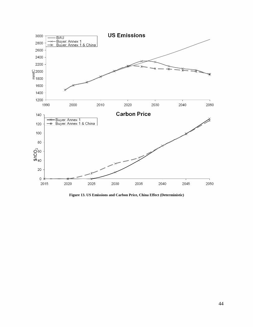
44

Figure 13. US Emissions and Carbon Price, China Effect (Deterministic)

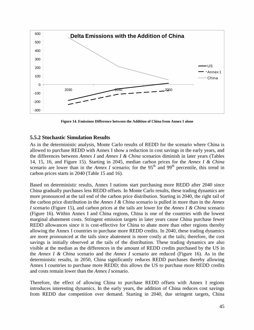
45

-300

-200

-100

0

100

200

300

400

500

600

2030 2040 2050

Delta Emissions with the Addition of China

US

Annex 1

China

Figure 14. Emissions Difference between the Addition of China from Annex I alone

5.5.2 Stochastic Simulation Results

As in the deterministic analysis, Monte Carlo results of REDD for the scenario where China is

allowed to purchase REDD with Annex I show a reduction in cost savings in the early years, and

the differences between Annex I and Annex I & China scenarios diminish in later years (Tables

14, 15, 16, and Figure 15). Starting in 2045, median carbon prices for the Annex I & China

scenario are lower than in the Annex I scenario; for the 95th

and 99th

percentile, this trend in

carbon prices starts in 2040 (Table 15 and 16).

Based on deterministic results, Annex I nations start purchasing more REDD after 2040 since

China gradually purchases less REDD offsets. In Monte Carlo results, these trading dynamics are

more pronounced at the tail end of the carbon price distribution. Starting in 2040, the right tail of

the carbon price distribution in the Annex I & China scenario is pulled in more than in the Annex

I scenario (Figure 15), and carbon prices at the tails are lower for the Annex I & China scenario

(Figure 16). Within Annex I and China regions, China is one of the countries with the lowest

marginal abatement costs. Stringent emission targets in later years cause China purchase fewer

REDD allowances since it is cost-effective for China to abate more than other regions thereby

allowing the Annex I countries to purchase more REDD credits. In 2040, these trading dynamics

are more pronounced at the tails since abatement is more costly at the tails; therefore, the cost

savings is initially observed at the tails of the distribution. These trading dynamics are also

visible at the median as the differences in the amount of REDD credits purchased by the US in

the Annex I & China scenario and the Annex I scenario are reduced (Figure 16). As in the

deterministic results, in 2050, China significantly reduces REDD purchases thereby allowing

Annex I countries to purchase more REDD; this allows the US to purchase more REDD credits

and costs remain lower than the Annex I scenario.

Therefore, the effect of allowing China to purchase REDD offsets with Annex I regions

introduces interesting dynamics. In the early years, the addition of China reduces cost savings

from REDD due competition over demand. Starting in 2040, due stringent targets, China

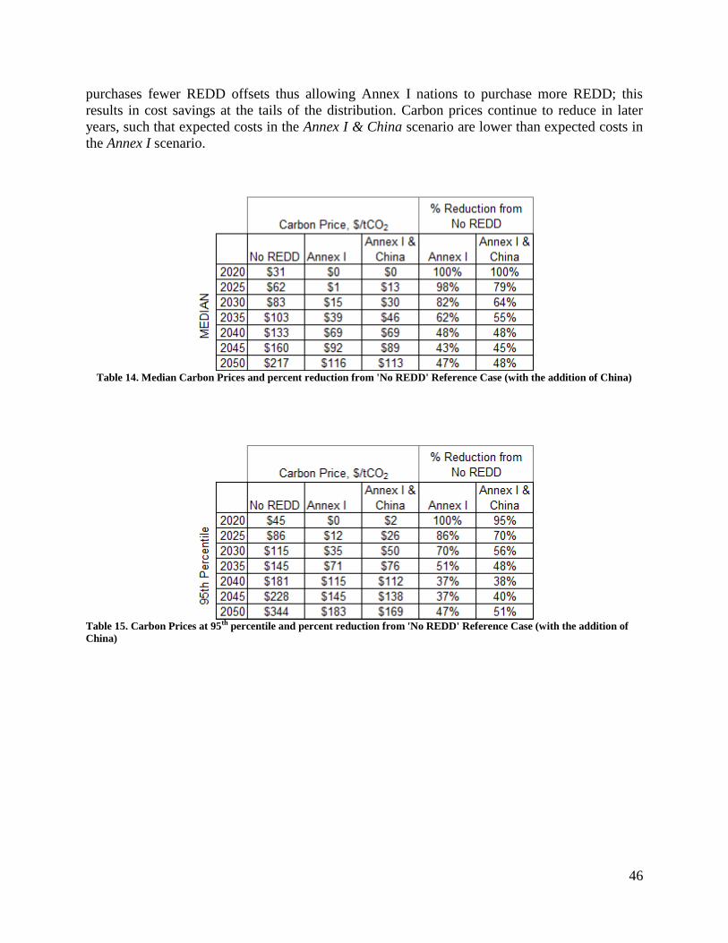
46

purchases fewer REDD offsets thus allowing Annex I nations to purchase more REDD; this

results in cost savings at the tails of the distribution. Carbon prices continue to reduce in later

years, such that expected costs in the Annex I & China scenario are lower than expected costs in

the Annex I scenario.

Table 14. Median Carbon Prices and percent reduction from 'No REDD' Reference Case (with the addition of China)

Table 15. Carbon Prices at 95th percentile and percent reduction from 'No REDD' Reference Case (with the addition of

China)

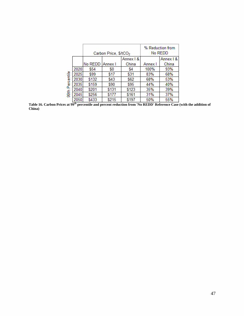
47

Table 16. Carbon Prices at 99th percentile and percent reduction from 'No REDD' Reference Case (with the addition of

China)

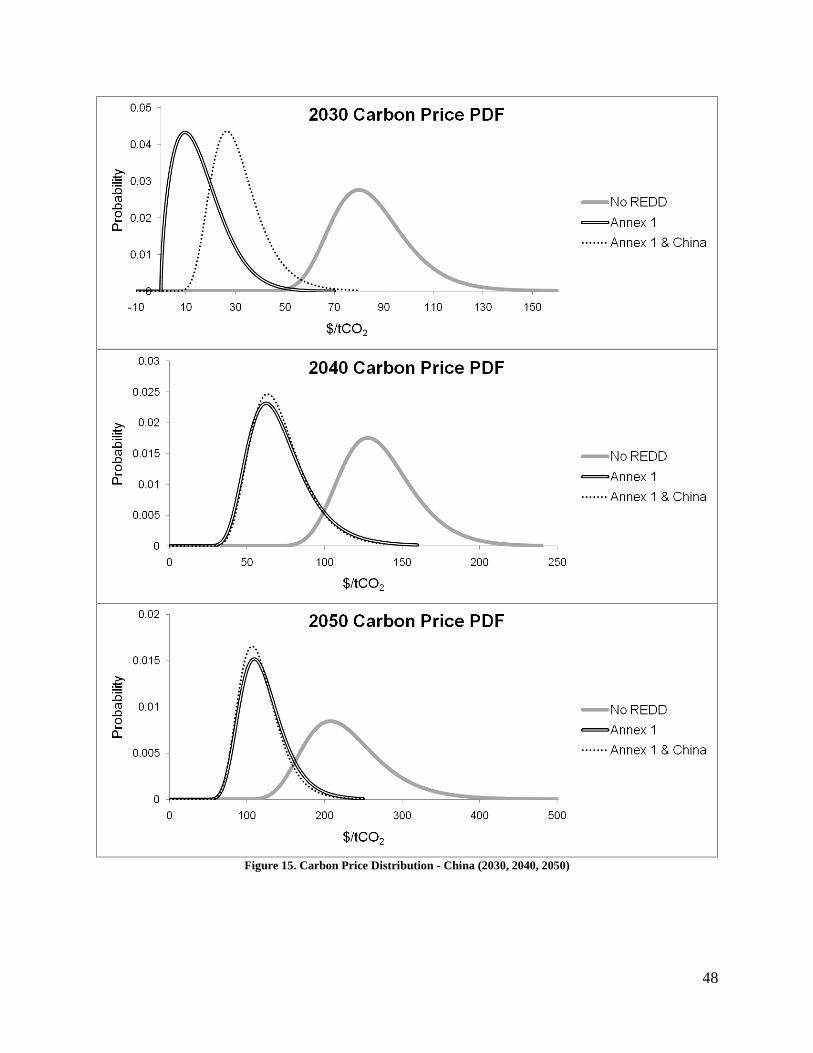
48

Figure 15. Carbon Price Distribution - China (2030, 2040, 2050)

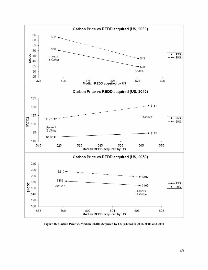
49

Figure 16. Carbon Price vs. Median REDD Acquired by US (China) in 2030, 2040, and 2050

50

6. Policy Implications Based on the analysis presented above, carbon offsets such as REDD not only will lower

expected costs, but also, have the potential to reduce upside carbon price uncertainties.

Therefore, carbon offsets can provide an alternative cost-containment flexibility mechanism in

climate change legislation. Carbon offsets are an attractive cost-containment instrument as it

does not involve using domestic allowances, and it incentivizes further global participation to

reduce global GHG emissions. In addition, growing demand for carbon offsets can increase

development aid for carbon offset producing nations. The demand for carbon offsets as a cost-

containment instrument would further incentivize the use of offsets in climate legislation, and

rising demand of offsets from developed nations would encourage efforts to further expand the

availability of more offsets, like REDD. In addition, the availability of REDD offsets in an

emissions trading scheme would allow developed nations to utilize otherwise unavailable

deforestation and forest degradation mitigation options thus providing the vital financial support

to considerably curb deforestation. In addition, the increased interest in REDD could spur the

development and standardization of monitoring and verification methods for REDD activities.

Therefore, carbon offsets can offer benefits for both developed and developing nations, thereby

promoting global participation.

Cost-containment instruments address a variety of cost uncertainties, such as start-up, short-term,

and long term uncertainties (Webster et al., 2008a). The ability of carbon offsets to address these

cost uncertainties depends on the supply of carbon offsets. Carbon offsets can address start-up

cost uncertainties if there is a sufficient supply of offsets available during the inception of an

emissions trading scheme. Short-term cost uncertainties can be addressed if carbon offsets are

available for specific short periods of time, and long-term uncertainties can be addressed if

carbon offset supply can be sustained for a long period of time.

Scarcity of offsets can reduce the cost-containment effectiveness, where scarcity can be affected

by changes in the demand for and the supply of offsets. Current assessments of the supply of

REDD offsets are based on assumptions of opportunity costs and deployment rates; therefore,

uncertainties in opportunity costs and deployment rates can make assessing supply difficult. As

shown in the results in Chapter 5, supply uncertainties due to uncertainties in opportunity costs

and deployment rates can significantly affect the effectiveness of REDD as a cost-containment

instrument. These uncertainties have the greatest impact in the early years thus affecting start-up

cost containment effectiveness. In addition, if there is significant inter-year supply variability,

this can limit short-term cost containment if carbon offset supply is too small to compensate for

high carbon prices.

Moreover, increased offset scarcities in later years may be inevitable. As discussed in Section

4.2, emission targets tend get more stringent in later years. Emission target trajectories are

typically constructed to be less stringent in earlier years to facilitate infrastructure changes, such

as technology investment, to meet future emission targets. These increasingly stringent emission

targets make offsets scarcer since stringent targets require purchasing larger amounts of offsets

to compensate for the larger emission reductions thereby increasing the demand for offsets.

Therefore, the effectiveness of offsets as a long-term cost-containment instrument will depend on

whether the supply of offsets can increase in later years to meet the increased demand. However,

51

opportunity costs for carbon offsets in later years are likely to increase as all low cost options are

likely to be exhausted early. As offset opportunity costs rise and domestic mitigation efforts

become cost competitive, the demand for carbon offsets will decrease as there are more cost-

effective options. The combination of stringent targets and higher opportunity costs in later years

reduces the likelihood for carbon offsets to address long-term price uncertainties effectively.

Therefore, carbon offsets are likely to be more effective at containing start-up and short-term

cost uncertainties, as long-term uncertainties are likely to persist due to stringent targets and

higher opportunity costs.

Since carbon offsets reduce expected costs, it can delay domestic abatement efforts like clean

energy and technology investments and can weaken consumer price signals to reduce energy

consumption. These concerns are often translated into offset purchasing restrictions, such as the

two billion metric ton CO2 offset restriction in Waxman-Markey. These offset purchasing

restrictions make offsets scarcer regionally; therefore, these restrictions can significantly reduce

the cost-containment effectiveness of offsets as demonstrated in the results in Chapter 5.

Alternatively, the Regional Greenhouse Gas Initiative (RGGI), a US Northeast and Mid-Atlantic

State GHG reduction initiative, incorporates offsets as a sort of allowance reserve mechanism,

where more offsets are allowed to enter the market when the trigger price is exceeded. RGGI

initially limits offsets to 3.3% of a unit‘s total compliance obligation during a control period. If

carbon prices exceed $7 (2005 dollars), allowed offsets increase to 5 percent, and if prices

exceed $10 (2005 dollars), allowed offsets increase to 10 percent. This allows carbon offsets to

primarily function as a cost-containment instrument for high carbon prices. The effectiveness of

this mechanism is highly dependent on the allocated trigger price; low trigger price essentially

allows carbon offsets to be available often, and an unrealistically high trigger price may never

allow additional offsets to enter the market. These restrictions may deal with the concerns of low

expected costs, but this can simultaneously reduce the supply of offsets, reducing participation

from developing nations and possibly delaying necessary funding to developing countries. These

purchasing restrictions significantly limit cost-containment for all three types of cost-

uncertainties, since demand is limited for all years.

Start-up cost containment is heavily impacted by offset purchasing restrictions and supply

uncertainties. If start-up cost uncertainties are particularly troublesome, supplementing offsets

with another cost-containment instrument and/or delaying offset purchasing restrictions to later

years may provide some relief.

Moreover, as more countries allow carbon offsets into their respective trading schemes,

competition for carbon offsets can make offsets scarcer. The European Emissions Trading

Scheme (EU ETS), which is the largest trading scheme in operation, has offset restrictions; these

restrictions can have a significant effect on the supply of carbon offsets to other countries. EU

ETS limits carbon offsets to non-forestry activities, and according to the draft amendment of the

EU ETS Directive, it is likely to be excluded post-Kyoto (Streck et al., 2009). Under this

scenario, a surplus of REDD allowances could exist for to non-European Union countries, which

would provide substantial cost savings and reduced risk of upside carbon price uncertainties for

non-European Union countries. However, competitiveness effects are significantly mitigated by

supply uncertainties and domestic offset purchasing restrictions. Therefore, competition over

52

offsets will likely play a minor role compared to regional offset purchasing restrictions and target

stringency.

Linking emission trading schemes is an attractive option as it helps lower expected costs by

taking advantage of lower abatement options among developed nations with emission

commitments. However, flexibility mechanisms, such as cost-containment instruments, can

complicate the linkage between trading schemes with divergent mechanisms. For example,

linking a US emissions trading scheme that accepts forestry credits with EU ETS can weaken EU

ETS restrictions on forestry credits; it would make forestry credits available in EU ETS thus

weakening EU restrictions. One way to address these concerns is to filter out incompatible

carbon offsets from the linked systems; this requires a comprehensive tracking system with

strong enforcement mechanisms to ensure that these offsets do not enter non-compliant trading

schemes, which will raise the transaction costs of the entire system.

For REDD, non-permanence further complicates linkage. Emission reductions from REDD may

be subjected to non-permanence from events such as forest fires. As a result, someone needs to

be responsible for maintaining permanence by restoring the released carbon. The designated

party liable for non-permanence plays a significant role in linked schemes. If the producer of

offsets is liable for non-permanence, linking is easy, provided that the trading systems to be

linked have consistent accounting and verification rules. However, if buyers are liable for non-

permanence, linking is complicated, especially when certain schemes do not allow REDD

offsets, as in EU ETS (Streck et al., 2009). Trading schemes with REDD restrictions will be less

inclined to link, but if they are linked, there must be provisions to track REDD credits to ensure

they are not traded with EU ETS. Even if both linked schemes accept REDD offsets, the means

of restoration needs to be subjected to verification, and each linked scheme should have standard

rules and enforcement capacity to ensure that integrity is maintained. In both cases of linked

systems, consistent standards are necessary as lax rules in one scheme can drive laxity

throughout the entire linked system thus weakening all other schemes (Streck et al., 2009). In

both cases, developed countries will need to work closely with offset producers to ensure and

develop consistent standards, especially in the case when the producer is responsible for

permanence.

Due to inherent supply uncertainties in carbon offsets, supplementing carbon offsets with other

cost-containment instruments is recommended. In many cases, carbon offsets are not

differentiated from domestic allowances and thus allowed to be banked as in the Waxman-

Markey Bill. Similar to banking of allowances, banking offsets add intertemporal flexibility to

the use of offsets; regions and sectors can defer the use of offsets for future years when targets

are stricter and abatement costs are higher. Allowing the banking of offsets can be used to

address longer term price uncertainties. However, banking offsets may increase the demand for

offsets as participants in schemes that allow banking may result in purchasing additional offsets

to bank thereby increasing offset scarcity for the years when banking is exercised. This increase

in demand can disrupt supply for other regions. Therefore, during the years when banking is

exercised, cost savings from REDD may be reduced as banking can make offsets globally scarce.

In addition, since carbon offsets could delay domestic abatement efforts, banking carbon offsets

may further delay abatement efforts as these banked offsets introduce additional low cost

abatement options in future years, displacing and delaying the otherwise adopted domestic

53

mitigation options. However, banking limitation provisions can be added to emissions trading

schemes to restrict how long a permit can be banked. In Waxman-Markey, there are proposed

expiration dates for offsets, which is a method to address these concerns. However, the

effectiveness of banking as a supplemental instrument can be significantly limited by restrictions

on offset purchases as these restrictions alone place significant limitations on cost-containment

based on results in Chapter 5.

For REDD, non-permanence issues can also complicate banking. REDD offsets would need to

be tracked and monitored to ensure that offsets are restored appropriately. In addition, if a REDD

offset needs to be restored in a future year, the restored offset may need to be discounted

depending on when the non-permanence occurs. The Waxman-Markey Bill allows borrowing

allowances with interest (8 percent per year); this interest rate or similar can be applied to

permanence activities. On the other hand, if the responsibility of permanence is on the producer

of the REDD offset, then these permanence details need to be accounted for by the producer.

Carbon offsets are attractive for industrialized countries since they are generally cheaper than

domestic abatement options. However, implementing carbon offsets requires additional

administrative support that can add costs. For example, tracking and monitoring carbon offsets to

ensure integrity within linked systems and within a scheme, especially in the case of banking and

non-permanence, can add transaction and administrative costs. The extent of costs depends on

who is liable for non-permanence and inconsistencies between linked systems that need to be

addressed. However, liability for non-permanence may not make a difference, if producer

liability costs are internalized in carbon offset opportunity costs.

This mechanism is just a temporary solution for price uncertainties, as these low cost carbon

offsets will eventually be exhausted and price uncertainties are likely to persist. However, unlike

more common cost-containment instruments, it does incentivize further involvement of

developing countries, which is necessary for large GHG reductions in the future, by funding

abatement projects via carbon offsets; these projects promote sustainable development hopefully

paving the way for real GHG emission reduction commitments from developing countries in the

near future.

In the end, increased use of carbon offsets to leverage cost-containment effects may be a mixed

blessing for developing countries. Carbon offsets can provide the necessary support to move

towards a more sustainable development path; however, when these developing countries move

towards actual emission reduction commitments, these low cost abatement options will likely be

exhausted. Therefore, there may be some equity concerns over abatement efforts as these

developed nations enter into agreements, which may result in restricted output of carbon offsets

to retain some of these options for the future. These supply restrictions will likely affect the cost-

containment effectiveness of carbon offsets.

54

7. Conclusion

In this paper, I investigated whether carbon offsets can reduce carbon price uncertainties,

specifically upside carbon prices. Because offset scarcity from changes in the demand for and

supply of offsets can impact cost containment effectiveness; I examined the following supply

and demand offset restriction scenarios on costs: (1) increasing competition over offset demand;

(2) offset purchasing restrictions, and (3) supply uncertainties. Using REDD as a case study

example, I analyzed these scenarios on REDD offsets in the EPPA model both deterministically

and stochastically.

The results confirm that REDD lowers expected costs and more importantly reduces upside

costs. Carbon prices at the 99th

percentile were found to have at least a 51 percent reduction from

the ‗No REDD‘ reference case. Increasing competition over the demand reduces the cost savings

from REDD, although the effect of competition is less pronounced in later years since emission

targets are more stringent in later years. In addition, US offset purchasing restrictions

substantially reduce cost containing effectiveness especially in the early years. Supply

uncertainties also reduce effectiveness but less than the US offset purchasing restriction.

Moreover, competition effects are muted in the presence of US offset purchasing restrictions and

supply uncertainties as these restrictions impact offset scarcity more than from competition.

Considering supply uncertainties and offset restrictions reduce effectiveness in the early years

and the combination of stringent targets and increasing offset opportunity costs in later years,

carbon offsets may be more effective at addressing short-term cost uncertainties.

Supplementing carbon offsets with another cost-containment instrument, such as banking, may

help address scarcity concerns and help address longer term cost uncertainties. On the other

hand, supplemental instruments may raise concerns about further delaying domestic action. In

addition, offset purchasing restrictions can reduce the effectiveness of additional cost-

containment instruments as offset scarcity can limit the amount of offsets that can be banked.

Carbon offsets can serve as an important cost-containment instrument that has the added benefit

of encouraging participation by developing nations through the support of sustainable

development activities in these developing nations. The demand for carbon offsets as a cost

containment instrument would encourage efforts to further expand the availability of more

offsets, like REDD, thereby further promoting the development and deployment of REDD

offsets. The inclusion of REDD credits in emissions trading schemes could provide the necessary

financial transfers to developing nations to substantially curb deforestation. However, offsets

restrictions in current and proposed legislations can significantly reduce magnitude of these

financial transfers.

Furthermore, incorporating carbon offsets to a trading scheme can add complications in linked

systems. For example, forestry offsets are not permitted in the EU ETS; therefore, linked

schemes need to be vigilant that these offsets do not leak into EU ETS thereby weakening EU

restrictions. In addition, ensuring permanence for REDD offsets will require standard rules and

verification methods to maintain integrity; these measures to ensure system integrity will add

transaction and administrative costs. Moreover, equity concerns from developing nations, that

55

low cost abatement options will be exhausted when they commit to actual emission reductions,

may result in offset supply restrictions, which can also affect cost-containment.

7.1 Future Work

Banking is a good supplemental instrument to carbon offsets as it can add inter-year flexibility

on the use of offsets; in fact, Waxman-Markey Bill allows the banking of offsets. In my model,

carbon offsets were bought and consumed at the same time; there was no re-trading or banking.

It would be interesting to simulate banking of offsets to understand the effects of banking on

cost-effectiveness.

As mentioned in Chapter 7, RGGI uses offsets as an allowance reserve instrument, where if the

trigger price is exceeded, more offsets are allowed to enter the system. It would be interesting to

analyze carbon offsets as an allowance reserve, with a sensitivity analysis on different allowance

reserve restrictions, such as trigger prices and offset quantities allowed. This can be compared to

the results from the US Waxman-Markey 1bmt international offset restriction.

For my initial REDD supply, I assumed that the maximum available REDD was where the costs

went vertical. It would be more realistic to insert the REDD MAC curves in EPPA, such that

REDD supply was determined by equating marginal costs between EPPA‘s MAC and REDD

MAC. This may involve linking forestry models, like GTM, with a forward-looking EPPA

model. The two models may need to run concurrently as the GTM model will need account for

the forestry abatement options exercised in the EPPA model, and the EPPA model will need

abatement costs from the GTM model to determine the share of abatement activity from the

forestry sector. Alternatively, forestry assumptions can be added into the EPPA model to

account for available forestry abatement opportunities.

56

References Asner, G. P., Knapp, D. E., Broadbent, E. N., Oliveira, P. J. C., Keller, M., Silva, J. N. (2005),

―Selective logging in the Brazilian Amazon‖, Science, Vol 310, pp 480–482

Barker T, Bashmakov I, Bernstein L et al (2007), Technical summary. In: Metz B, Davidson OR,

Bosch PR (eds) Climate change 2007: mitigation. Contribution of working group III to

the fourth assessment report of the Intergovernmental Panel on Climate Change.

Cambridge University Press, UK

Corbera, E., Estrada, M., Brown, K. (2009), ―Reducing greenhouse gas emissions from

deforestation and forest degradation in developing countries: revisiting the assumptions‖,

Climactic Change, DOI 10.1007/s10584-009-9773-1

Dale, V. H., Joyce, L. A., McNulty, S., Neilson, R. P., Ayres, M. P., Flannigan, M. D., Hanson,

P. J., Irland, L. C., Lugo, A. E., Peterson, C. J., Simberloff, D., Swanson, F. J., Stocks, B.

J., Wotton, B. M. (2001), ―Climate change and forest disturbances‖, Bioscience, Vol. 51,

pp 723–734

Dimaranan, B. and R. McDougall, 2002: Global Trade, Assistance, and Production: The GTAP 5

Data Base. Center for Global Trade Analysis, Purdue University, West Lafayette,

Indiana.

Eliasch J. (2008), ―Climate change: financing global forests‖, Eliasch review

Ellerman, A. D., Jacoby, H. D., Decaux, A. (1998), ―The Effects on Developing Countries of the

Kyoto Protocol and Carbon Dioxide Emissions Trading‖, World Bank Policy Research,

Working Paper 2019

Fell, H., MacKenzie, I.A., Pizer, W. A. (2008), ―Prices versus Quantities versus Bankable

Quantities‖, Resources for the Future”, Discussion Paper

G8 Summit (2009) – Climate Change Fact Sheet

http://www.g8italia2009.it/static/G8_Allegato/Fact%20Sheet%20-

%20Climate%20Change%20(ENG).pdf

Geist H and Lambin E (2001), ―What drives tropical deforestation? A meta-analysis of

proximate and underlying causes of deforestation based on subnational case study

evidence‖. LUCC (Land Use and Land Use Cover Change) Project Report Series No. 4.

Belgium: Louvain-la-Neuve

Hertel, T., 1997: Global Trade Analysis: Modeling and Applications. Cambridge University

Press, Cambridge: United Kingdom.

Houghton RA (2005), ―Tropical deforestation as a source of greenhouse gas emissions.‖, In:

http://www.g8italia2009.it/static/G8_Allegato/Fact%20Sheet%20-%20Climate%20Change%20(ENG).pdf

http://www.g8italia2009.it/static/G8_Allegato/Fact%20Sheet%20-%20Climate%20Change%20(ENG).pdf

57

Moutinho P, Schwartzman S (eds) Tropical deforestation and climate change. IPAM and

Environmental Defense, Belem

Hyman, R.C., J.M. Reilly, M.H. Babiker, A. De Masin and H.D. Jacoby, 2003: Modeling Non-

CO2 Greenhouse Gas Abatement. Environmental Modeling and Assessment, 8(3): 175-

186; MIT Joint Program Reprint 2003-9.

Intergovernmental Panel on Climate Change (IPCC) (2007), Climate Change 2007: Synthesis

Report. Intergovernmental Panel on Climate Change Fourth Assessment Report (AR4).

Kindermann, G., Obersteiner, M., Sohngen, B., Sathaye, J., Andrasko, K., Rametsteiner, E.,

Schlamadinger, B., Wunder, S., Beach, R., (2008), ―Global cost estimates of reducing

carbon emissions through avoided deforestation‖, Proceedings of the National Academy

of Sciences of the United States of America, Vol. 105, pp 10302-10307

MacKerron, G. J., Egerton, C., Gaskell, C., Parpia, A., Mourato, S. (2009), ―Willingness to pay

for carbon offset certification and co-benefits among (high-)flying young adults in the

UK‖, Energy Policy, Vol. 37, pp 1372-1381.

Mathiesen, L. (1985): Computation of Economic Equilibrium by a Sequence of Linear

Complementarity Problems. Mathematical Programming Study, 23,144-162.

Morris, J., Paltsev, S., Reilly, J. (2008), ―Marginal Abatement Costs and Marginal Welfare Costs

for Greenhouse Gas Emissions Reductions: Results from the EPPA Model‖, MIT Joint

Program on the Science and Policy of Global Change, Report 164,

http://globalchange.mit.edu/pubs/abstract.php?publication_id=972

Murray, B. C., Newell, R. G., Pizer, W. A. (2008), ―Balancing Cost and Emissions Certainty: An

Allowance Reserve for Cap-and-Trade‖, National Bureau of Economic Research,

Working Paper 14258, http://www.nber.org/papers/w14258

Murray, B., Lubowski R., Sohngen, B., (2009) ―Including International Forest Carbon Incentives

in Climate Policy: Understanding the Economics‖, Nicholas Institute Report

Newell R. and Pizer, W. A. (2003), ―Regulating stock externalities under uncertainty‖, Journal

of Environmental and Economics Management”, Vol. 45, pp 416-432

Niles, J. O., Brown, S., Pretty, J., Ball, A. S., Fay, J. (2002), " Potential carbon mitigation and

income in developing countries from changes in use and management of agricultural and

forest lands‖, Philosophical Transactions of the Royal Society Biological Sciences, Vol.

360, pp 1621-1639

O‘Brien, Karen L (2000) ―Upscaling Tropical Deforestation: Implications for Climate Change‖,

Climactic Change, Vol. 44, pp 311-329.


http://www.nber.org/papers/w14258

58

Paltsev, S., J.M. Reilly, H.D. Jacoby, R.S. Eckaus, J. McFarland, M. Sarofim, M. Asadoorian

and M. Babiker, (2005): The MIT Emissions Prediction and Policy Analysis (EPPA)

Model: Version 4. MIT Joint Program on the Science and Policy of Global Change

Report 125. http://web.mit.edu/globalchange/www/MITJPSPGC_Rpt125.pdf.

Pizer, W. A. (2002). ―Combining price and quantity controls to mitigate global climate change,‖

Journal of Public Economics, Vol 85, pp 409-434.

Roberts, M. J. and Spence, M (1976), ―Effluent Charges and Licenses under Uncertainty‖,

Journal of Public Economics, Vol. 5, pp 193-208.

Rosenbaum, K. L., Schöne, D., Mekouar, A. (2004), ―Climate change and the forest sector—

possible national and subnational legislation‖, FAO forestry paper. FAO, Rome

Rutherford, T.F. (1995): Extension of GAMS for Complementarity Problems Arising in Applied

Economic Analysis. Journal of Economic Dynamics and Control, 19(8): 1299-1324.

Stavins, R (2004), The Political Economy of Environmental Regulation, Edward Elgar

Publishing Limited, Northampton, MA.

Stern N (2006) Stern review: the economics of climate change. Cambridge University Press,

Cambridge

Stoll-Kleeman, S., Bender, S., Berghöfer, A.; Bertzky, M.; Fritz-Vietta, N. Schliep, R.;

Thierfelder, B. (2006) ―Linking governance and management perspectives with

conservation success in protected areas and biosphere reserves‖, Discussion paper 01 of

the Governance and Biodiversity Research Group, Humboldt-Universität zu Berlin

Streck, C., Tuerk, A., Schlamadinger, B. (2009), ―Foresty offsets in emissions trading systems: a

link between systems?‖, Mitigation and Adaptation Strategies for Global Change, Vol.

14, pp 455-463

Tavoni, M., Sohngen, B., Bosetti, V. (2006), ―Forestry and the carbon market response to

stabilize climate‖, Energy Policy, Vol. 35, pp 5346-5353

Tole, L. (1998), ―Sources of Deforestation in Tropical Developing Countries‖, Environmental

Management, Vol. 22, pp 19-33

United Nations Framework Convention on Climate Change Seventh Session of the Conference

of Parties (COP 7) (2002), Marrakesh Accord,

http://unfccc.int/resource/docs/cop7/13.pdf

United Nations Framework Convention on Climate Change Thirteenth Session of the Conference

of Parties (COP 7) (2008), Bali Action Plan,

http://unfccc.int/resource/docs/2007/cop13/eng/06a01.pdf

http://web.mit.edu/globalchange/www/MITJPSPGC_Rpt125.pdf

http://unfccc.int/resource/docs/cop7/13.pdf

http://unfccc.int/resource/docs/2007/cop13/eng/06a01.pdf

59

United Nations Framework Convention on Climate Change Fifteenth Session of the Conference

of Parties (COP 15) (2009), Copenhagen Accord,

http://www.denmark.dk/NR/rdonlyres/C41B62AB-4688-4ACE-BB7B-

F6D2C8AAEC20/0/copenhagen_accord.pdf

United Nations Framework Convention on Climate Change (1998), Kyoto Protocol.

http://unfccc.int/resource/docs/convkp/kpeng.pdf

The United States Congressional Budget Office (2008), A CBO Study: Policy Options for

Reducing CO2 Emissions

United States Environmental Protection Agency (2008), EPA Analysis of the Lieberman-Warner

Climate Security Act of 2008.

http://www.epa.gov/climatechange/downloads/s2191_EPA_Analysis.pdf

United States Environmental Protection Agency (1963), The Clean Air Act

http://www.epa.gov/air/caa/

United States Environmental Protection Agency (2010), Supplemental EPA Analysis of the

American Clean Energy and Security Act of 2009.

http://www.epa.gov/climatechange/economics/pdfs/HR2454_SupplementalAnalysis_App

endix.pdf

van‘t Veld, K., Plantinga, A. (2004), ―Carbon sequestration or abatement? The effect of rising

carbon prices on the optimal portfolio of greenhouse-gas mitigation strategies‖, Journal

of Environmental Economics and Management, Vol. 50, pp 59-81

Vattenfall (2007) ―Global mapping of greenhouse gas abatement opportunities up to 2030,

forestry sector deep-dive‖

Wagner, G., Keohane, N., Petsonk, A., Wang, J., (2009), ―Docking into a global carbon market:

Clean Investment Budgets to finance low-carbon economic development‖,

Environmental Defense Fund

Watson, R. T., Noble, I. R., Bolin, B., Ravindranath, N. H., Verardo, D. J., Dokken, D. J. (2000),

―Land use, land-use change, and forestry‖. A special report of the Intergovernmental

Panel on Climate Change. Cambridge University Press, UK

Waxman, H. and Markey, E. (2009), The American Clean Energy and Security Act of 2009, H.R.

2454

Webster, M. D., Parsons, J., Ellerman, A. D., Jacoby, H. (2008a), ―Cost Containment: A Primer‖

in ―Cap-and-Trade: Contributions to the Design of a U.S. Greenhouse Gas Program‖,

MIT Center for Energy and Environmental Policy Research, pp 36-58

Webster, M., Paltsev, S., Parsons, J., Reilly, J., Jacoby, H. (2008b) ―Uncertainty in Greenhouse

http://www.denmark.dk/NR/rdonlyres/C41B62AB-4688-4ACE-BB7B-F6D2C8AAEC20/0/copenhagen_accord.pdf

http://www.denmark.dk/NR/rdonlyres/C41B62AB-4688-4ACE-BB7B-F6D2C8AAEC20/0/copenhagen_accord.pdf

http://unfccc.int/resource/docs/convkp/kpeng.pdf

http://www.epa.gov/climatechange/downloads/s2191_EPA_Analysis.pdf

http://www.epa.gov/air/caa/

http://www.epa.gov/climatechange/economics/pdfs/HR2454_SupplementalAnalysis_Appendix.pdf

http://www.epa.gov/climatechange/economics/pdfs/HR2454_SupplementalAnalysis_Appendix.pdf

60

Gas Emissions and Costs of Atmospheric Stabilization‖, MIT Joint Program on the

Science and Policy of Global Change, Report 165,


Weitzman, M. (1974), ―Price vs. Quantities‖, The Review of Economic Studies, Vol. 41, pp 471-

491


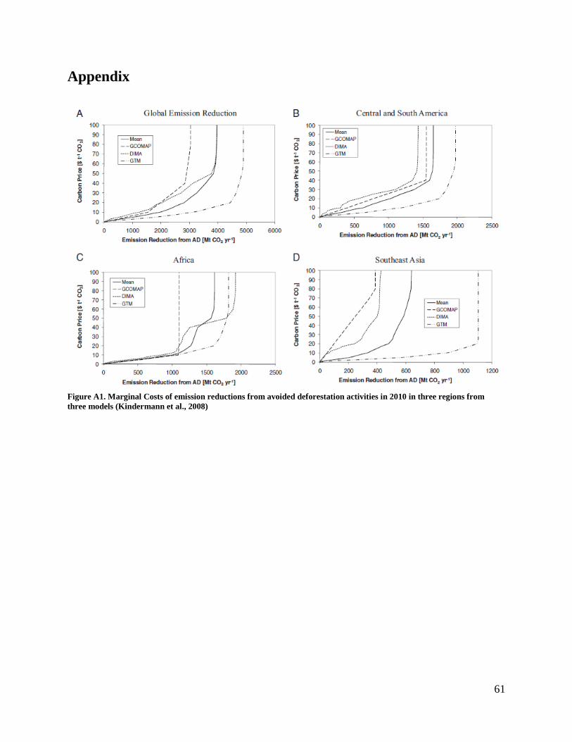
61

Appendix

Figure A1. Marginal Costs of emission reductions from avoided deforestation activities in 2010 in three regions from

three models (Kindermann et al., 2008)

62

Figure A2. Marginal Costs of emission reductions from avoided deforestation activities in 2030 in three regions from

three models (Kindermann et al., 2008)

Figure A3. Carbon Price vs. Median REDD Acquired by US (China) in 2020

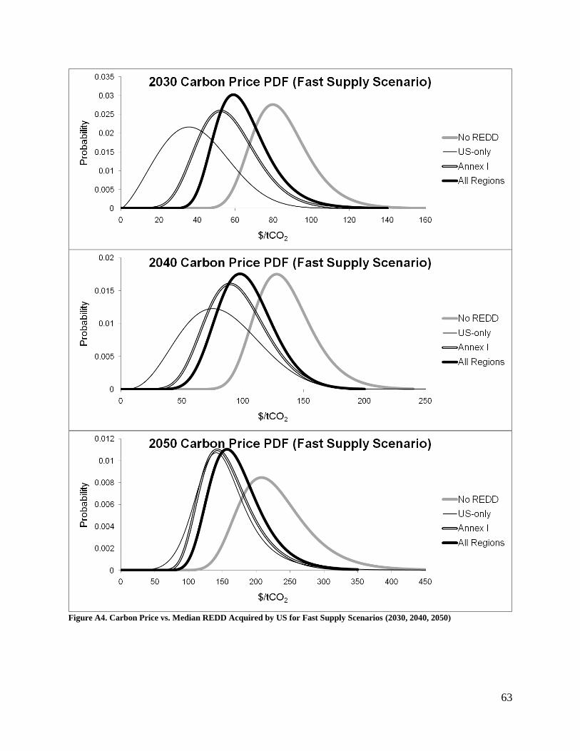
63

Figure A4. Carbon Price vs. Median REDD Acquired by US for Fast Supply Scenarios (2030, 2040, 2050)

64

Figure A5. Carbon Price vs. Median REDD Acquired by US for Fast Supply Scenarios (2030, 2040, 2050)

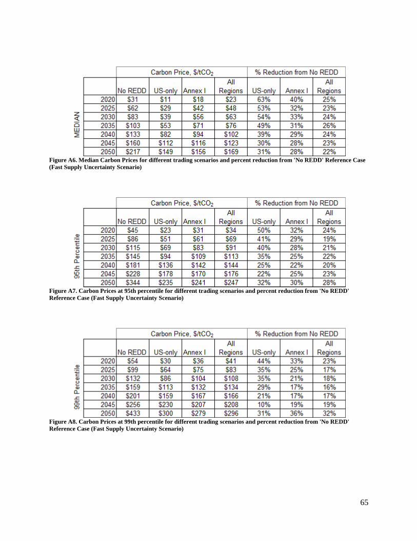
65

Figure A6. Median Carbon Prices for different trading scenarios and percent reduction from 'No REDD' Reference Case

(Fast Supply Uncertainty Scenario)

Figure A7. Carbon Prices at 95th percentile for different trading scenarios and percent reduction from 'No REDD'

Reference Case (Fast Supply Uncertainty Scenario)

Figure A8. Carbon Prices at 99th percentile for different trading scenarios and percent reduction from 'No REDD'

Reference Case (Fast Supply Uncertainty Scenario)

Documents

Carbon Offsets as a Cost Containment Instrument: A Case