Embed Size (px)
Citation preview
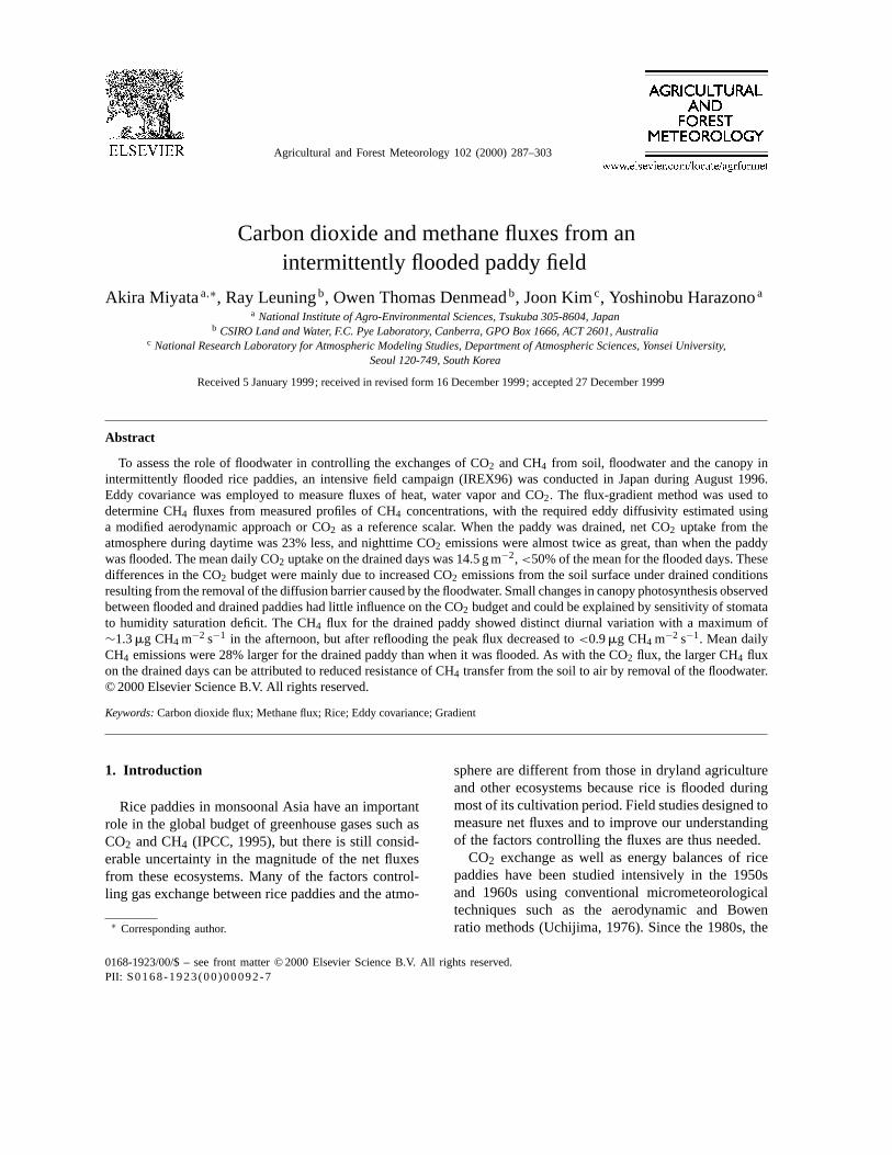
Agricultural and Forest Meteorology 102 (2000) 287–303
Carbon dioxide and methane fluxes from anintermittently flooded paddy field
Akira Miyataa,∗, Ray Leuningb, Owen Thomas Denmeadb, Joon Kimc, Yoshinobu Harazonoaa National Institute of Agro-Environmental Sciences, Tsukuba 305-8604, Japan
b CSIRO Land and Water, F.C. Pye Laboratory, Canberra, GPO Box 1666, ACT 2601, Australiac National Research Laboratory for Atmospheric Modeling Studies, Department of Atmospheric Sciences, Yonsei University,
Seoul 120-749, South Korea
Received 5 January 1999; received in revised form 16 December 1999; accepted 27 December 1999
Abstract
To assess the role of floodwater in controlling the exchanges of CO2 and CH4 from soil, floodwater and the canopy inintermittently flooded rice paddies, an intensive field campaign (IREX96) was conducted in Japan during August 1996.Eddy covariance was employed to measure fluxes of heat, water vapor and CO2. The flux-gradient method was used todetermine CH4 fluxes from measured profiles of CH4 concentrations, with the required eddy diffusivity estimated usinga modified aerodynamic approach or CO2 as a reference scalar. When the paddy was drained, net CO2 uptake from theatmosphere during daytime was 23% less, and nighttime CO2 emissions were almost twice as great, than when the paddywas flooded. The mean daily CO2 uptake on the drained days was 14.5 g m−2, <50% of the mean for the flooded days. Thesedifferences in the CO2 budget were mainly due to increased CO2 emissions from the soil surface under drained conditionsresulting from the removal of the diffusion barrier caused by the floodwater. Small changes in canopy photosynthesis observedbetween flooded and drained paddies had little influence on the CO2 budget and could be explained by sensitivity of stomatato humidity saturation deficit. The CH4 flux for the drained paddy showed distinct diurnal variation with a maximum of∼1.3mg CH4 m−2 s−1 in the afternoon, but after reflooding the peak flux decreased to<0.9mg CH4 m−2 s−1. Mean dailyCH4 emissions were 28% larger for the drained paddy than when it was flooded. As with the CO2 flux, the larger CH4 fluxon the drained days can be attributed to reduced resistance of CH4 transfer from the soil to air by removal of the floodwater.© 2000 Elsevier Science B.V. All rights reserved.
Keywords:Carbon dioxide flux; Methane flux; Rice; Eddy covariance; Gradient
1. Introduction
Rice paddies in monsoonal Asia have an importantrole in the global budget of greenhouse gases such asCO2 and CH4 (IPCC, 1995), but there is still consid-erable uncertainty in the magnitude of the net fluxesfrom these ecosystems. Many of the factors control-ling gas exchange between rice paddies and the atmo-
∗ Corresponding author.
sphere are different from those in dryland agricultureand other ecosystems because rice is flooded duringmost of its cultivation period. Field studies designed tomeasure net fluxes and to improve our understandingof the factors controlling the fluxes are thus needed.
CO2 exchange as well as energy balances of ricepaddies have been studied intensively in the 1950sand 1960s using conventional micrometeorologicaltechniques such as the aerodynamic and Bowenratio methods (Uchijima, 1976). Since the 1980s, the
0168-1923/00/$ – see front matter © 2000 Elsevier Science B.V. All rights reserved.PII: S0168-1923(00)00092-7
288 A. Miyata et al. / Agricultural and Forest Meteorology 102 (2000) 287–303
development of fast response CO2 analyzers enabledus to measure CO2 fluxes over a rice canopy by theeddy covariance method (Ohtaki and Matsui, 1982;Ohtaki, 1984), which gave us more reliable flux esti-mates than before. However, the mechanism of CO2exchange between rice paddies and the atmosphere isnot fully understood. For example, using eddy covari-ance measurements, Tsukamoto (1993) found a sig-nificantly smaller net CO2 flux from the atmosphereto a rice canopy when the field was drained com-pared to when it was flooded, but the reason for thedifference was not clear. The existence of floodwater,anaerobic soil or changes in the micrometeorologicalenvironment with flooding will influence root activity,photosynthesis and respiration of rice plants. Activityof aquatic plants such as algae in the floodwater mayalso affect CO2 exchange between rice paddies andthe atmosphere. Many of the data obtained so far arenot sufficiently detailed to examine the influence ofthese factors on the CO2 exchange in rice paddies.
Paddy fields are also one of largest sources in theglobal budget of CH4. Based on incubation experi-ments in a laboratory, Koyama (1963) first estimatedthe CH4 production rate by world rice production tobe 190 Tg per year. Since the 1980s there have beennumerous field measurements of CH4 fluxes in variousrice paddies over the world (e.g. Cicerone and Shet-ter, 1981; Holzapfel-Pschorn and Seiler, 1986; Schützet al., 1989; Sass et al., 1990; Yagi and Minami, 1990;Khalil et al., 1998), leading to revised estimates of theglobal CH4 emission from rice paddies of 60 Tg peryear, but with uncertainty ranging from 20 to 100 Tgper year (IPCC, 1995).
Most estimates of CH4 fluxes have used chambersplaced over plants, soil and paddy water, but chambersdisturb the environment during measurement. Severalpioneering studies on net CH4 fluxes over rice pad-dies using non-disturbing micrometeorological meth-ods have now been made (Denmead, 1991; Simpsonet al., 1995; Harazono et al., 1996). The flux-gradientapproach was used in these studies rather than theeddy covariance technique because, unlike for CO2,fast-response gas analyzers for CH4 have not beenavailable until very recently. Eddy covariance mea-surements using tunable diode laser absorption spec-troscopy are now becoming available (Verma et al.,1992; Shurpali et al., 1993; Edwards et al., 1994; Kimet al., 1998a, b).
Net exchanges of CO2 and CH4 between rice pad-dies and the atmosphere are controlled by several bi-ological and physical processes. During the daytimeplant photosynthesis leads to uptake of CO2 fromboth the atmosphere and from respired CO2 emit-ted by the soil and floodwater. Respiration at nightleads to an efflux of CO2 to the atmosphere. CH4is released to the atmosphere by ebullition, diffusionacross the water-air interface and by transport throughaerenchyma, well-developed intracellular air spaceswhich supply atmospheric oxygen from pores in theleaves, through the plant stems, and to the roots of therice plants (Nouchi, 1994). Up to 90% of CH4 emis-sion occurs through the aerenchyma in undisturbedpaddy fields (Minami and Neue, 1994).
To improve understanding of the process control-ling CO2 and CH4 exchanges in rice paddies, anintensive field experiment called IREX96 (the 1996International Rice Experiment) was conducted inJapan during August 1996. In this paper, we presentmeasurements of CO2 and CH4 fluxes over a ricecanopy obtained using micrometeorological tech-niques; eddy covariance for CO2 and flux-gradientmethods for CH4. The measurements were used toassess the role of floodwater in controlling the ex-changes of CO2 and CH4 from the soil, the floodwaterand the plant canopy. Factors controlling exchangeprocesses are examined further in a companion pa-per (Leuning et al., 2000), where we estimate sourcestrength distributions for CO2 and CH4 within therice using an analysis of turbulent dispersion andmeasured concentration profiles.
2. CH444 flux measurement using flux-gradienttheory
Methane fluxes over the rice canopy were measuredusing two methods based on flux-gradient theory; anaerodynamic method and a gradient technique whichuses the eddy covariance flux of CO2, a referencescalar (tracer). These methods have been used conven-tionally for the measurement of fluxes of gases as wellas sensible heat and latent heat (e.g. Inoue et al., 1958,1969). In this study we used a modified aerodynamicmethod (Harazono and Miyata, 1997), and there-fore it is instructive to describe here the methods indetail.
A. Miyata et al. / Agricultural and Forest Meteorology 102 (2000) 287–303 289
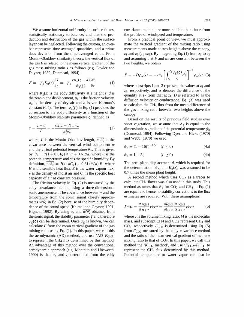
We assume horizontal uniformity in surface fluxes,statistically stationary turbulence, and that the pro-duction and destruction of the gas within the surfacelayer can be neglected. Following the custom, an over-bar represents time-averaged quantities, and a primedoes deviation from the time-averaged value. FromMonin–Obukhov similarity theory, the vertical flux ofthe gasF is related to the mean vertical gradient of thegas mass mixing ratios as follows (e.g. Fowler andDuyzer, 1989; Denmead, 1994):
F = −ρaKg(z)∂s
∂z= −ρa
κu∗(z − d)
φg(ζ )
∂s
∂z(1)
whereKg(z) is the eddy diffusivity at a heightz, d isthe zero-plane displacement,u∗ is the friction velocity,ρa is the density of dry air andκ is von Karman’sconstant (0.4). The termφg(ζ ) in Eq. (1) provides thecorrection to the eddy diffusivity as a function of theMonin–Obukhov stability parameterζ , defined as
ζ = z − d
L= −κg(z − d)w′θ ′
v
u3∗θ ′v
(2)
where,L is the Monin–Obukhov length,w′θ ′v is the
covariance between the vertical wind componentwand the virtual potential temperatureθv. This is givenby, θv = θ(1 + 0.61q) ≈ θ + 0.61θq, whereθ is thepotential temperature andq is the specific humidity. Bydefinition, w′θ ′
v = H/(ρCp
) + 0.61(θ/ρ
)E, where
H is the sensible heat flux,E is the water vapour flux,ρ is the density of moist air andCp is the specific heatcapacity of air at constant pressure.
The friction velocity in Eq. (2) is measured by theeddy covariance method using a three-dimensionalsonic anemometer. The covariance betweenw and thetemperature from the sonic signal closely approxi-matesw′θ ′
v in Eq. (2) because of the humidity depen-dence of the sound speed (Kaimal and Gaynor, 1991;Hignett, 1992). By usingu∗ andw′θ ′
v obtained fromthe sonic signal, the stability parameterζ and thereforeφg(ζ ) can be determined. Onceφg is known, we cancalculateF from the mean vertical gradient of the gasmixing ratio using Eq. (1). In this paper, we call thisthe aerodynamic (AD) method, and use ‘AD–FCH4’to represent the CH4 flux determined by this method.An advantage of this method over the conventionalaerodynamic approach (e.g. Monteith and Unsworth,1990) is thatu∗ and ζ determined from the eddy
covariance method are more reliable than those fromthe profiles of windspeed and temperature.
From a practical point of view, we must approxi-mate the vertical gradient of the mixing ratio usingmeasurements made at two heights above the canopy,z1 andz2 (z1<z2). By integrating Eq. (1) fromz1 to z2and assuming thatF andu∗ are constant between thetwo heights, we obtain
F = −Dρa1s = −κu∗[∫ ζ2
ζ1
φg(ζ )
ζdζ
]−1
ρa1s (3)
where subscripts 1 and 2 represent the values atz1 andz2, respectively, and1 denotes the difference of thequantity atz2 from that atz1. D is referred to as thediffusion velocity or conductance. Eq. (3) was usedto calculate the CH4 flux from the mean difference ofthe gas mixing ratio between two heights above thecanopy.
Based on the results of previous field studies overshort vegetation, we assume thatφg is equal to thedimensionless gradient of the potential temperatureφh(Denmead, 1994). Following Dyer and Hicks (1970)and Webb (1970) we used:
φh = (1 − 16ζ )−1/2 (ζ ≤ 0) (4a)
φh = 1 + 5ζ (ζ ≥ 0) (4b)
The zero-plane displacementd, which is required forthe determination ofζ andKg(z), was assumed to be0.7 times the mean plant height.
A second method which uses CO2 as a tracer tocalculate CH4 fluxes was also used in this study. Thismethod assumes thatφg for CO2 and CH4 in Eq. (1)are equal and hence no stability corrections to the fluxestimates are required. With these assumptions
FCH4 = 1sCH4
1sCO2FCO2 = MCH4
MCO2
1cCH4
1cCO2FCO2 (5)
wherec is the volume mixing ratio,M is the molecularmass, and subscript CH4 and CO2 represent CH4 andCO2, respectively.FCH4 is determined using Eq. (5)from FCO2 measured by the eddy covariance methodand the ratio of the mean vertical gradient of methanemixing ratio to that of CO2. In this paper, we call thismethod the ‘KCO2 method’, and use ‘KCO2–FCH4’ torepresent the CH4 flux determined by this method.Potential temperature or water vapor can also be
290 A. Miyata et al. / Agricultural and Forest Meteorology 102 (2000) 287–303
used as a reference scalar instead of CO2. Thesetracer methods are advisable particularly when thenighttime fluxes are being investigated because calmperiods may invalidate the aerodynamic approach(Denmead, 1994). In this study, we choose CO2 as atracer because the nighttime vertical gradients of CO2mixing ratio can be measured more accurately thanthose of potential temperature or water vapor.
3. Experimental
3.1. Site description
IREX96 was conducted at the Hachihama experi-mental farm of Okayama University, Japan (34◦32′N,133◦56′E, 2 m above sea level). The farm, approx-imately 300 m×300 m, is situated in a paddy areawithin reclaimed land facing Kojima Bay in the south-ern part of Okayama Prefecture. The soil is mainly clay(>60%; Kobashi et al., 1968). Rice cultivation on thefarm has continued in a similar way every year since1960. In 1996 rice (Oryza sativaL.; cultivar Akebono)was seeded to the dry paddy on 13 May with densityof 60 kg ha−1 and a row spacing of 27 cm. Irrigationstarted on 19 June and the field was flooded continu-ously until 12 July. This was followed by an intermit-tent drainage practice with 4 days of flooding and 3days drainage which continued until harvest on 30 Oc-tober. This intermittent drainage is aimed at removingsalt from the paddy fields. Neither compost nor ricestraw were applied to the paddy, but slow-release-typemineral fertilizers (N, P, K=77, 77, 77 kg ha−1) wereapplied at the time of seeding. The dry matter yield of1996 was 5930 kg ha−1, which was 25% greater thanthe average yield from 1989 to 1995 (4740 kg ha−1).
The measurement of CO2 and CH4 fluxes over thecanopy was conducted from 6 to 13 of August, about amonth before heading of the rice plants on 5 Septem-ber. The paddy was drained from the afternoon of 6August to the morning of 9 August, and was floodedto a depth of 8–10 cm for the remaining observationperiod. The plant height was about 0.72 m above thewater surface, and the leaf area index (LAI) measuredwith a canopy analyzer (LAI-2000, LICOR Inc., Lin-coln, NE, USA) was 3.08±0.28 (the mean±standarddeviation) with a spatial variability from 1.6 to 3.9.Yamamoto et al. (1995) showed LAIs of rice plants
measured with the canopy analyzer agreed well withthose by destructive measurement (standard error was0.28).
Micrometeorological sensors and air inlets weremounted on the masts at the center of the experi-mental farm. The fetch in the prevailing SE directionexceeded 300 m, and footprint analysis followingSchuepp et al. (1990) indicated that >90% of themeasured flux at a height of 2.2 m was expected tocome from within the nearest 300 m of upwind area(Harazono et al., 1998).
3.2. Eddy covariance measurements
Friction velocityu∗, and the fluxes of sensible heatH, water vaporE, and CO2 FCO2, over the rice canopywere measured by the eddy covariance method. Theeddy covariance method has been widely used forCO2 flux measurements above plant canopies anda useful summary of the technique can be found inLeuning and Judd (1996). A three-dimensional sonicanemometer (Solent, Model 1012R, Gill InstrumentsLtd., Lymington, UK) with path length of 15 cm wasinstalled at a height of 2.2 m above the water to mea-sure the fluctuations of three components of windvelocity. Fluctuations in virtual temperature wereobtained from the vertical axis signal of the sonicanemometer (Kaimal and Gaynor, 1991; Hignett,1992). To measure fluctuations in the CO2 and wa-ter vapor concentrations, a fast response infrared gasanalyzer with a 20 cm span open-path (E009, Ad-vanet Inc., Okayama, Japan) was installed at the sameheight as the sonic anemometer with a horizontal sep-aration of 17 cm. The sensitivity of the gas analyzerto CO2 was calibrated before and after the experi-ment using three levels of standard gases (between300 and 400 ppmv CO2 in N2, Takachiho ChemicalIndustrial Co. Ltd., Tokyo, Japan). The sensitivity ofthe analyzer to water vapor was factory-calibrated ina thermostatic chamber before the experiment. Thedata from the sonic anemometer and the gas ana-lyzer were sampled at 10 Hz using a 16-bit digitaldata recorder (DR-M2a, TEAC Co., Ltd., Tokyo,Japan).
The fluxes u∗, H, E and FCO2 were calculatedon a 30 min basis from the covariances between thevertical wind velocity and corresponding quantities.A correction for path length averaging of the sonic
A. Miyata et al. / Agricultural and Forest Meteorology 102 (2000) 287–303 291
anemometer and the gas analyzer, and that for sepa-ration of both sensors were applied following Moore(1986) and Leuning and Moncrieff (1990). The in-fluence of these corrections on each flux varies withatmospheric stability, but the average magnitudes ofthe corrections are as follows. The correction for pathlength averaging increasedu∗ andH by 0.5 and 2.9%,respectively, while corrections for path length averag-ing plus sensor separation increasedE and FCO2 by11.8 and 12.6%, respectively. The influence of densityfluctuations arising fromH andE (Webb et al., 1980)increasedE by 4.9% and reducedFCO2 by 10.1%.Because we calibrated the CO2 sensor using CO2 innitrogen (i.e. dry conditions), we were unable to de-termine the cross-sensitivity of the CO2 gas analyzerto water vapor (Leuning and Moncrieff, 1990). Hadwe applied the correction with the cross-sensitivityfound for their E009 instrument (β/α=1×10−3 in Eq.(8) of Leuning and Moncrieff (1990)), the magnitudeof FCO2 would increase by 8.8% on average.
3.3. Measurement of gas concentration profiles
CH4 concentrations in sampled air were mea-sured using a non-dispersive infrared CH4 analyzer(GA-360E, Horiba Co. Ltd., Kyoto, Japan) equippedwith a specially designed pre-conditioner to minimizethe interference of non-methane hydrocarbons andwater vapor (Harazono et al., 1995). The time con-stant of the analyzer was 8.5 s. The CH4 analyzer wascalibrated twice a day, around 0900 and 1700 hoursusing two reference cylinders with high grade air con-taining 1.7 ppmv CH4 (Takachiho; certified accuracyis ±2%). CO2 concentrations were measured usinga non-dispersive infrared CO2 analyzer (LI-6251,LICOR), which was operated with a time constantof 1 s. The CO2 analyzer was calibrated at the sametime as the CH4 analyzer using two cylinders with350 and 400 ppmv CO2 in N2 (Takachiho).
Air inlets for sample air were mounted at eightheights, 0.12, 0.24, 0.36, 0.48, 0.60, 0.72, 1.10 and2.40 m above the water, and another inlet for refer-ence air was mounted at 2.50 m. The reference airwas required because the gas analyzers were operatedin the differential mode which detected the differ-ences in infrared absorption between the sample airand the reference air. The gas concentrations at 1.10and 2.40 m were used for the gas flux calculation by
use of the gradient method, while the whole profileswere used to infer sources and sinks of the gases inthe canopy using an inverse Lagrangian analysis asdescribed by Leuning et al. (2000). Teflon diaphragmpumps (MAA-P108-HB, Gas Manufacturing Corp.,Benton harbor, MI., USA) and nylon tubing (10 mmID) were used for air sampling. Air sampled at eachinlet was drawn through an ice-trap to reduce mois-ture content, into a cylindrical PVC buffer (70 dm3 involume; time constant is about 15 min), then pumpedto a T-junction, one arm of which was connected to atube placed in a 60 cm deep water bubbler to controlthe pressure and the flow rate in the sampling line.The third arm of each T-junction was connected toa solenoid valve to permit selection of each air linein turn for gas analysis. The solenoid valves werecontrolled by a data logger and a personal computer.The air in the selected line passed through flow me-ters, dried further to a dew point temperature of 2◦Cusing a Peltier-cooled condenser (DH-209, KomatsuElectronics Inc., Tokyo, Japan), and then analyzed.The solenoid valve was switched every 2 min, and thesampling sequence was as follows: Line 1 (2.4 m),2, 3, 4, 5, 6, 7, 8 (0.12 m), 7, 6, 5, 4, 3, 2, 1. . . .The full sampling sequence was thus completed in30 min. This ‘staircase’ sampling technique eliminateslinear trends in measurement of gas concentrationdifferences.
Gas concentration data were sampled and recordedevery 5 s using an A/D converter (Green Kit-88,Electric Systems Development, Tokyo, Japan) and apersonal computer. The mean of the data sampledbetween 30 and 110 s after line switching was usedto estimate the concentration at each height. After1730 hours of 11 August, however, the CH4 concen-tration was averaged between 80 and 110 s after lineswitching because the CH4 analyzer was operatedin the slow mode with a time constant of 26 s. Theinfluence of insufficient response of the CH4 analyzerin the slow mode on the average was estimated tobe less than 3%, and was neglected. The standarderror of the fluctuation of the analyzer’s output dur-ing the averaging period was 2.5 ppbv for the CH4analyzer in the fast mode, 1.0 ppbv in the slow modeand 0.2 ppmv for the CO2 analyzer. These standarderrors were used to estimate uncertainties in calcu-lated gas fluxes. The mean vertical difference of thegas concentration was calculated from 30 min means
292 A. Miyata et al. / Agricultural and Forest Meteorology 102 (2000) 287–303
(the average of consecutive two cycles of the profilemeasurement) at 1.10 and 2.40 m.
3.4. Chamber measurement of CH4 flux
CH4 fluxes were also measured using a closedchamber for comparison with the flux-gradientmethod. A bottom-less chamber, 0.36 m2 in area, 1 min height, made of acrylic resin, with an electric fanfor circulation was employed for the measurement.Details of the chamber and air sampling method aredescribed in Yagi and Minami (1993). The measure-ment was conducted on 13 August at two sites in themeasurement plot, approximately 20 m to the west(western site) and 30 m to the east of the masts (east-ern site). At each site, two chambers were placed4 m apart to examine the spatial variation of the flux.Air temperature inside the chamberTc and soil tem-perature below it were monitored using thermistorthermometers. Air was sampled four times at 10 minintervals by pumping air into a Tedlar bag (GL Sci-ence, Tokyo, Japan). The chamber was placed 5 minbefore the first air sampling, and was removed imme-diately after the last (forth) sampling. Volume mixingratios of CH4 in the bags were analyzed using agas chromatograph with a flame-ionization detec-tor (GC-9A, Shimadzu, Kyoto, Japan) located in anair-conditioned laboratory. The volume mixing ratiowas converted to density usingTc and the partialpressure of dry air in the chamberpa. The CH4 fluxwas deduced from the rate of change of CH4 den-sity with time as determined using linear regression.Leakage into the chamber caused by air sampling hadan insignificant effect on the flux measurement be-cause sampling removed∼1% (4 dm3) of the chambervolume.
3.5. Supplementary measurements
Incident and reflected solar radiation, net radiationand photosynthetically active radiation were measuredrespectively with an Epply-type pyranometer (MR-22,Eko, Tokyo, Japan), a net radiometer (Q*6, RadiationEnergy Balance Systems Inc., Seattle, WA, USA) anda quantum sensor (ML-020P, Eko). Soil heat flux wasmeasured by three heat flux plates (MF-81, Eko), andthe influence of the difference of thermal conductiv-ity between the plate (0.21 W m−1 K−1) and the soil
(ca. 1.0 W m−1 K−1) was corrected following Philip(1961). Water and soil temperatures (at 2 and 5 cmdepth) were measured with T-type thermocouples.Changes in heat storage in floodwater was estimatedfrom the change of water temperature. Water depthwas measured with a float-type water gauge. The ver-tical profiles of air temperature and relative humiditywere measured using ventilated Platinum resistancetemperature sensors and capacitive humidity sen-sors (HUMITTER® 50Y, Vaisala, Helsinki, Finland)mounted at the same heights as the air inlets.
3.6. Floodwater depth and meteorological conditions
Water depth started decreasing in the morning of 6August by drainage, and standing water disappearedat 1400 hours (Fig. 1a). Irrigation started at 0900 hoursof 9 August, and water depth reached 10 cm aroundmidday. The water level was maintained until theafternoon of 11 August, and afterwards graduallydecreased with cessation of irrigation.
Clear days continued during the experiment, butmeteorological conditions were a little different fromday to day (Fig. 1). Wind direction (not shown in thefigure) was constant, southeast, and windspeed showedclear diurnal variation: 2–3 m s−1 in the daytime (ex-cept on 12 and 13 August), and declined to less than0.5 m s−1 at night (Fig. 1b). On 12 and 13 August,windspeed was higher than on the other days as the re-sult of an approaching typhoon. The daily maximumair temperature at 2.4 m was 30–32◦C, and the dailyminimum was 23–26◦C (Fig. 1c). Saturation deficit ofair increased gradually in the morning, and reacheda maximum of 9–15 g kg−1 in the late afternoon. On10–11 August, higher air temperature and larger sat-uration deficit prevailed.
As shown in Fig. 1d, most of the net radiation in thedaytime was partitioned into latent heat fluxλE (λ islatent heat of vaporization of water), whereasH wasless than 50 W m−2 except on windy 13 August whenit exceeded 80 W m−2. H changed sign from positive(upward transport) in the morning to negative in the af-ternoon. The Bowen ratio (H/λE) on drained days (7–8August ) was 0.08 on average for 0900–1500 hours,while on flooded days (10–12 August) it ranged from−0.03 to 0.04. Further details of the energy bal-ance during IREX96 are given by Harazono et al.(1998).
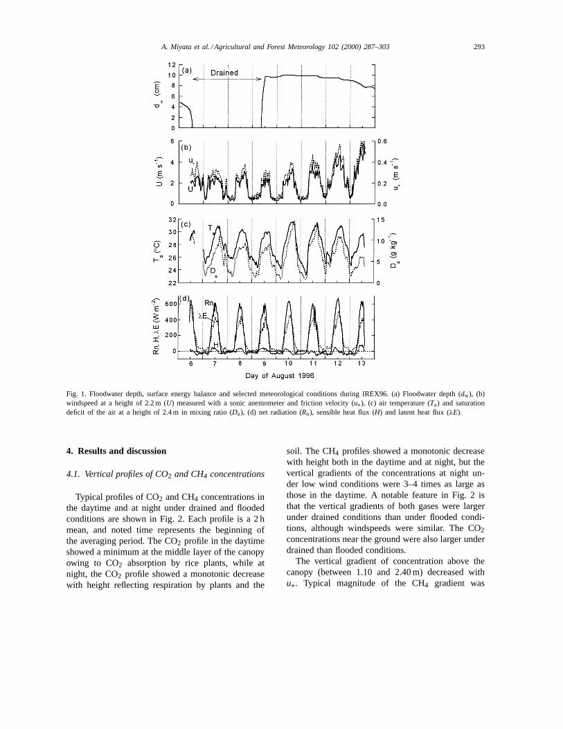
A. Miyata et al. / Agricultural and Forest Meteorology 102 (2000) 287–303 293
Fig. 1. Floodwater depth, surface energy balance and selected meteorological conditions during IREX96. (a) Floodwater depth (dw), (b)windspeed at a height of 2.2 m (U) measured with a sonic anemometer and friction velocity (u∗), (c) air temperature (Ta) and saturationdeficit of the air at a height of 2.4 m in mixing ratio (Da), (d) net radiation (Rn), sensible heat flux (H) and latent heat flux (λE).
4. Results and discussion
4.1. Vertical profiles of CO2 and CH4 concentrations
Typical profiles of CO2 and CH4 concentrations inthe daytime and at night under drained and floodedconditions are shown in Fig. 2. Each profile is a 2 hmean, and noted time represents the beginning ofthe averaging period. The CO2 profile in the daytimeshowed a minimum at the middle layer of the canopyowing to CO2 absorption by rice plants, while atnight, the CO2 profile showed a monotonic decreasewith height reflecting respiration by plants and the
soil. The CH4 profiles showed a monotonic decreasewith height both in the daytime and at night, but thevertical gradients of the concentrations at night un-der low wind conditions were 3–4 times as large asthose in the daytime. A notable feature in Fig. 2 isthat the vertical gradients of both gases were largerunder drained conditions than under flooded condi-tions, although windspeeds were similar. The CO2concentrations near the ground were also larger underdrained than flooded conditions.
The vertical gradient of concentration above thecanopy (between 1.10 and 2.40 m) decreased withu∗. Typical magnitude of the CH4 gradient was

294 A. Miyata et al. / Agricultural and Forest Meteorology 102 (2000) 287–303
Fig. 2. Examples of vertical profiles of CO2 (upper figures) and CH4 concentrations (lower figures) at a rice paddy in the daytime andat night. Each profile shows 2 h means of the difference from the concentration at 2.2 m. Closed circles indicate profiles under floodedcondition with a depth of 10 cm, and open circles indicate profiles under drained condition.hc indicates canopy height. Beginning time ofthe averaging period and the mean horizontal windspeed are shown at the top of the figure.
15 ppbv m−1 at u∗ of 0.2 m s−1, and 10 ppbv m−1
at 0.3 m s−1. The gradient increased markedly up to220 ppbv m−1 under stable atmospheric conditionswith u∗<0.1 m s−1.
4.2. CO2 fluxes under drained and flooded conditions
The time course of CO2 fluxes above the canopymeasured by the eddy covariance method (FCO2) isshown in Fig. 3. Also shown are the time courses ofair temperature within the canopy and soil temper-atures at 2 and 5 cm depth. Missing data forFCO2
are mainly due to the open-path infrared gas analyzerbeing out of range at night. The differences in noc-turnal FCO2 between drained and flooded conditionsare clearly shown in Fig. 3a. The nocturnalFCO2under drained conditions (from 7 to 8 August) was0.41±0.07 mg CO2 m−2 s−1 (the mean±the standarddeviation; 1900–0500 hours), whereas under floodedconditions (from 9 to 13 August) it was 0.19±0.06 mgCO2 m−2 s−1. The nocturnalFCO2 under floodedconditions are within the range of aboveground ricerespiration rate measured by chambers about a monthbefore heading (0.1–0.3 mg CO2 m−2 s−1; Yamaguchi
A. Miyata et al. / Agricultural and Forest Meteorology 102 (2000) 287–303 295
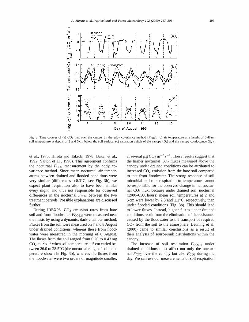
Fig. 3. Time courses of (a) CO2 flux over the canopy by the eddy covariance method (FCO2), (b) air temperature at a height of 0.48 m,soil temperature at depths of 2 and 5 cm below the soil surface, (c) saturation deficit of the canopy (Ds) and the canopy conductance (Gc).
et al., 1975; Hirota and Takeda, 1978; Baker et al.,1992; Saitoh et al., 1998). This agreement confirmsthe nocturnalFCO2 measurement by the eddy co-variance method. Since mean nocturnal air temper-atures between drained and flooded conditions werevery similar (differences<0.3◦C; see Fig. 3b), weexpect plant respiration also to have been similarevery night, and thus not responsible for observeddifferences in the nocturnalFCO2 between the twotreatment periods. Possible explanations are discussedfurther.
During IREX96, CO2 emission rates from baresoil and from floodwater,FCO2,S were measured nearthe masts by using a dynamic, dark-chamber method.Fluxes from the soil were measured on 7 and 8 Augustunder drained conditions, whereas those from flood-water were measured in the morning of 6 August.The fluxes from the soil ranged from 0.20 to 0.43 mgCO2 m−2 s−1 when soil temperature at 5 cm varied be-tween 26.0 to 28.5◦C (the nocturnal range of soil tem-perature shown in Fig. 3b), whereas the fluxes fromthe floodwater were two orders of magnitude smaller,
at severalmg CO2 m−2 s−1. These results suggest thatthe higher nocturnal CO2 fluxes measured above thecanopy under drained conditions can be attributed toincreased CO2 emission from the bare soil comparedto that from floodwater. The strong response of soilmicrobial and root respiration to temperature cannotbe responsible for the observed change in net noctur-nal CO2 flux, because under drained soil, nocturnal(1900–0500 hours) mean soil temperatures at 2 and5 cm were lower by 2.3 and 1.1◦C, respectively, thanunder flooded conditions (Fig. 3b). This should leadto lower fluxes. Instead, higher fluxes under drainedconditions result from the elimination of the resistancecaused by the floodwater to the transport of respiredCO2 from the soil to the atmosphere. Leuning et al.(2000) came to similar conclusions as a result oftheir analysis of source/sink distributions within thecanopy.
The increase of soil respirationFCO2,S underdrained conditions must affect not only the noctur-nal FCO2 over the canopy but alsoFCO2 during theday. We can use our measurements of soil respiration
296 A. Miyata et al. / Agricultural and Forest Meteorology 102 (2000) 287–303
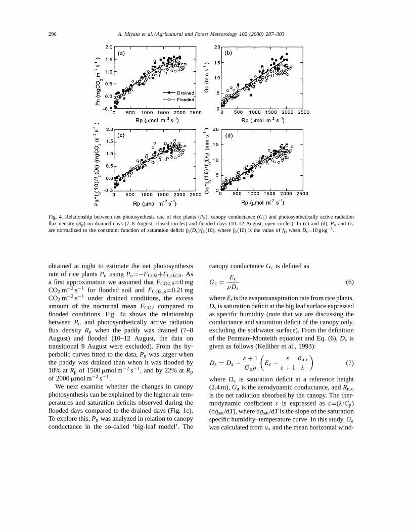
Fig. 4. Relationship between net photosynthesis rate of rice plants (Pn), canopy conductance (Gc) and photosynthetically active radiationflux density (Rp) on drained days (7–8 August; closed circles) and flooded days (10–12 August; open circles). In (c) and (d),Pn and Gc
are normalized to the constraint function of saturation deficitfD(Ds)/fD(10), wherefD(10) is the value offD when Ds=10 g kg−1.
obtained at night to estimate the net photosynthesisrate of rice plantsPn usingPn=−FCO2+FCO2,S. Asa first approximation we assumed thatFCO2,S=0 mgCO2 m−2 s−1 for flooded soil andFCO2,S=0.21 mgCO2 m−2 s−1 under drained conditions, the excessamount of the nocturnal meanFCO2 compared toflooded conditions. Fig. 4a shows the relationshipbetweenPn and photosynthetically active radiationflux density Rp when the paddy was drained (7–8August) and flooded (10–12 August, the data ontransitional 9 August were excluded). From the hy-perbolic curves fitted to the data,Pn was larger whenthe paddy was drained than when it was flooded by18% atRp of 1500mmol m−2 s−1, and by 22% atRpof 2000mmol m−2 s−1.
We next examine whether the changes in canopyphotosynthesis can be explained by the higher air tem-peratures and saturation deficits observed during theflooded days compared to the drained days (Fig. 1c).To explore this,Pn was analyzed in relation to canopyconductance in the so-called ‘big-leaf model’. The
canopy conductanceGc is defined as
Gc = Ec
ρDs(6)
whereEcis the evapotranspiration rate from rice plants,Ds is saturation deficit at the big leaf surface expressedas specific humidity (note that we are discussing theconductance and saturation deficit of the canopy only,excluding the soil/water surface). From the definitionof the Penman–Monteith equation and Eq. (6),Ds isgiven as follows (Kelliher et al., 1993):
Ds = Da − ε + 1
Gaρ
(Ec − ε
ε + 1
Rn,c
λ
)(7)
where Da is saturation deficit at a reference height(2.4 m),Ga is the aerodynamic conductance, andRn,cis the net radiation absorbed by the canopy. The ther-modynamic coefficientε is expressed asε=(λ/Cp)(dqsat/dT), where dqsat/dT is the slope of the saturationspecific humidity–temperature curve. In this study,Gawas calculated fromu∗ and the mean horizontal wind-
A. Miyata et al. / Agricultural and Forest Meteorology 102 (2000) 287–303 297
speedU at a height of 2.2 m such asGa=u∗2/U. Rn,cwas calculated from the extinction coefficient of netradiation by the rice canopy (0.66; Uchijima, 1961)and LAI. Ec was calculated asE–Es, whereEs is theevaporation rate from the soil/water surface which wasestimated from the available energy at the soil/watersurface (Leuning et al., 2000). The estimatedEc was84%, on average, of the total water vapor flux mea-sured above the canopyE, both for drained and floodedconditions, and the ratio is in good agreement with aprevious study (86% at LAI=3.08; Uchijima, 1961).
DaytimeGa ranged from 10 to 60 mm s−1, excepton 12 and 13 August when it was windy andGa in-creased up to 70 mm s−1. As shown in Fig. 3c, valuesof Ds in the daytime were generally<10 g kg−1, butin the afternoon of 10 and 11 August,Ds exceeded13 g kg−1. As a result,Gc around noon of these twodays was 12–13 mm s−1, compared to peak values of14–18 mm s−1 on other days. On the windy day of 13August,Gc at midday exceeded 21 mm s−1 whenDswas small.
The relationship betweenGc and Rp (Fig. 4b)shows that canopy conductances on flooded dayswere smaller than drained days at the sameRp level.To examine the influence of saturation deficit onGcquantitatively, we utilize constraint functions follow-ing Jarvis (1976) and Schulze et al. (1995):
Gc = Gc,maxfR
(RP
)fD (Ds) fT (T1) (8)
whereGc,max is the value ofGc without constraints,and the functionsfR, fD and fT (between 0 and 1) ac-count for the constraints onGc,max imposed by, irra-diance,Ds and leaf temperatureTl , respectively. As afirst approximation we assumed thatfT = 1 (no con-straint) and thatfD has the hyperbolic form
fD (Ds) = 1
1 + Ds/Ds,1/2(9)
whereDs,1/2 is the value ofDs at whichGc=Gc,max/2.We assumed a typical value ofDs,1/2=10 g kg−1 (Le-uning, 1995), and normalized bothPn and Gc to astandard humidity deficit of 10 g kg−1 through mul-tiplying by the factorfD (10)/fD (Ds). It is accept-able to normalizePn by this factor as well because itis relatively insensitive to changes inDs (see Leun-ing, 1995). Relationships between the normalizedPnand Gc as a function ofRp (Fig. 4c and d, respec-tively) now show little difference between the flooded
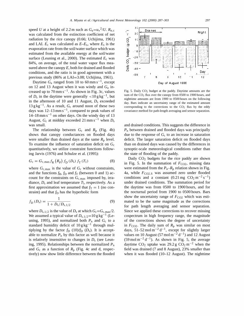
Fig. 5. Daily CO2 budget at the paddy. Daytime amounts are thesum of the CO2 flux over the canopy from 0500 to 1900 hours, andnighttime amounts are from 1900 to 0500 hours on the followingday. Bars indicate an uncertainty range of the estimated amountcorresponding to the corrections to the CO2 flux by the eddycovariance method for path-length averaging and sensor separation.
and drained conditions. This suggests the difference inPn between drained and flooded days was principallydue to the response ofGc to an increase in saturationdeficit. The larger saturation deficit on flooded daysthan on drained days was caused by the differences insynoptic-scale meteorological conditions rather thanthe state of flooding of the paddy.
Daily CO2 budgets for the rice paddy are shownin Fig. 5. In the summation ofFCO2, missing datawere estimated from thePn–Rp relation shown in Fig.4a, while FCO2,S was assumed zero under floodedconditions and a constant (0.21 mg CO2 m−2 s−1)under drained conditions. The summation period forthe daytime was from 0500 to 1900 hours, and forthe nocturnal period from 1900 to 0500 hours. Barsshow the uncertainty range ofFCO2 which was esti-mated to be the same magnitude as the correctionsfor path length averaging and sensor separation.Since we applied these corrections to recover missingcospectrum in high frequency range, the magnitudeof the corrections shows the degree of uncertaintyin FCO2. The daily sum ofRp was similar on mostdays, 51–52 mol m−2 d−1, except for slightly largervalues on 10 August (57 mol m−2 d−1) and 12 August(59 mol m−2 d−1). As shown in Fig. 5, the averagedaytime CO2 uptake was 29.2 g CO2 m−2 when thefield was drained (7 and 8 August), 23% smaller thanwhen it was flooded (10–12 August). The nighttime
298 A. Miyata et al. / Agricultural and Forest Meteorology 102 (2000) 287–303
CO2 emission on the drained days, on the other hand,was 14.7 mg CO2 m−2, which was almost twice asmuch as on the flooded days. As a result, the averagenet daily (24 h) CO2 uptake on the drained days was14.5 g CO2 m−2, while it was 29.8 g CO2 m−2 on theflooded days. As described earlier, these differencesin the CO2 budget between the two treatment periodsare mainly due to differences in the rate of CO2 re-lease from the soil surface, and to a lesser extent thereduction of plant photosynthesis due to the largersaturation deficit on flooded days.
A previous study on the same site and at a similarrice growth stage (Tsukamoto, 1993, 1994) showedthat the net downward CO2 flux between 0500 and1900 hours was 33% smaller when the field wasdrained than when it was flooded with 10 cm of wa-ter. The IREX96 results are similar to this study, andit is now clear that the decrease in the net daytimedownward CO2 flux under drained conditions wascaused by an increase of CO2 emission from the soilsurface. In the short term, intermittent drainage thusreduces net CO2 uptake from the atmosphere by ricepaddies compared to continuously flooded paddies.
4.3. CH4 fluxes under drained and flooded conditions
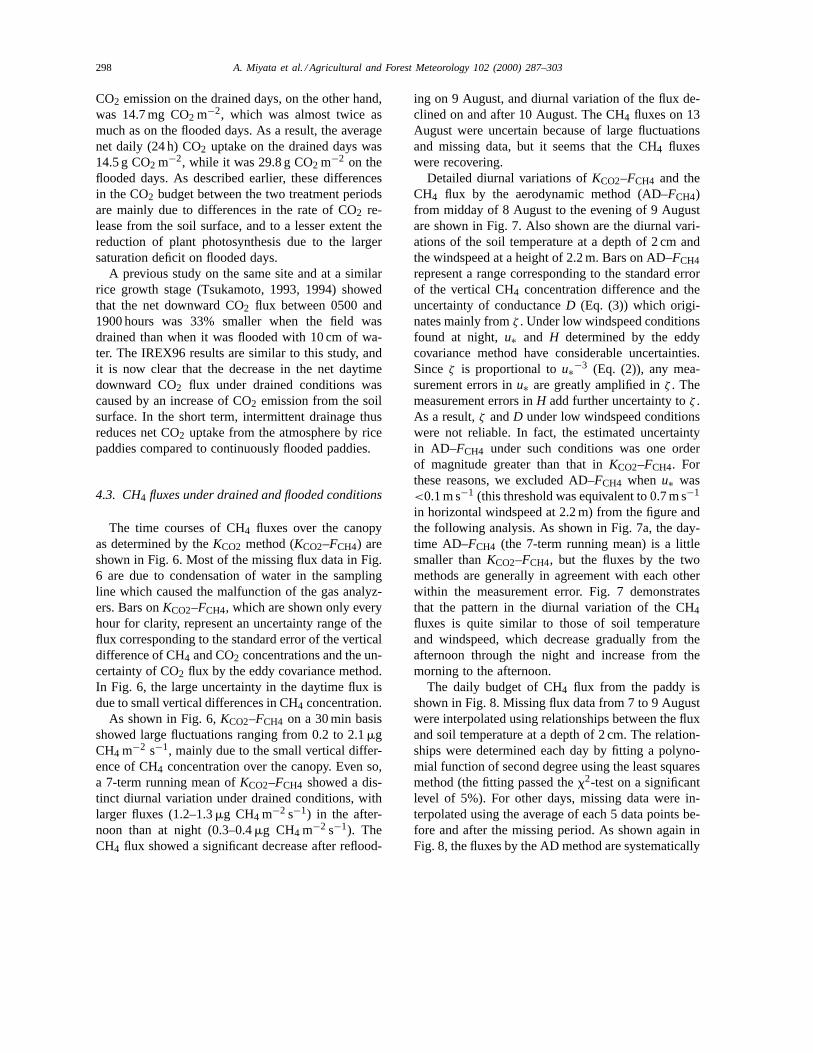
The time courses of CH4 fluxes over the canopyas determined by theKCO2 method (KCO2–FCH4) areshown in Fig. 6. Most of the missing flux data in Fig.6 are due to condensation of water in the samplingline which caused the malfunction of the gas analyz-ers. Bars onKCO2–FCH4, which are shown only everyhour for clarity, represent an uncertainty range of theflux corresponding to the standard error of the verticaldifference of CH4 and CO2 concentrations and the un-certainty of CO2 flux by the eddy covariance method.In Fig. 6, the large uncertainty in the daytime flux isdue to small vertical differences in CH4 concentration.
As shown in Fig. 6,KCO2–FCH4 on a 30 min basisshowed large fluctuations ranging from 0.2 to 2.1mgCH4 m−2 s−1, mainly due to the small vertical differ-ence of CH4 concentration over the canopy. Even so,a 7-term running mean ofKCO2–FCH4 showed a dis-tinct diurnal variation under drained conditions, withlarger fluxes (1.2–1.3mg CH4 m−2 s−1) in the after-noon than at night (0.3–0.4mg CH4 m−2 s−1). TheCH4 flux showed a significant decrease after reflood-
ing on 9 August, and diurnal variation of the flux de-clined on and after 10 August. The CH4 fluxes on 13August were uncertain because of large fluctuationsand missing data, but it seems that the CH4 fluxeswere recovering.
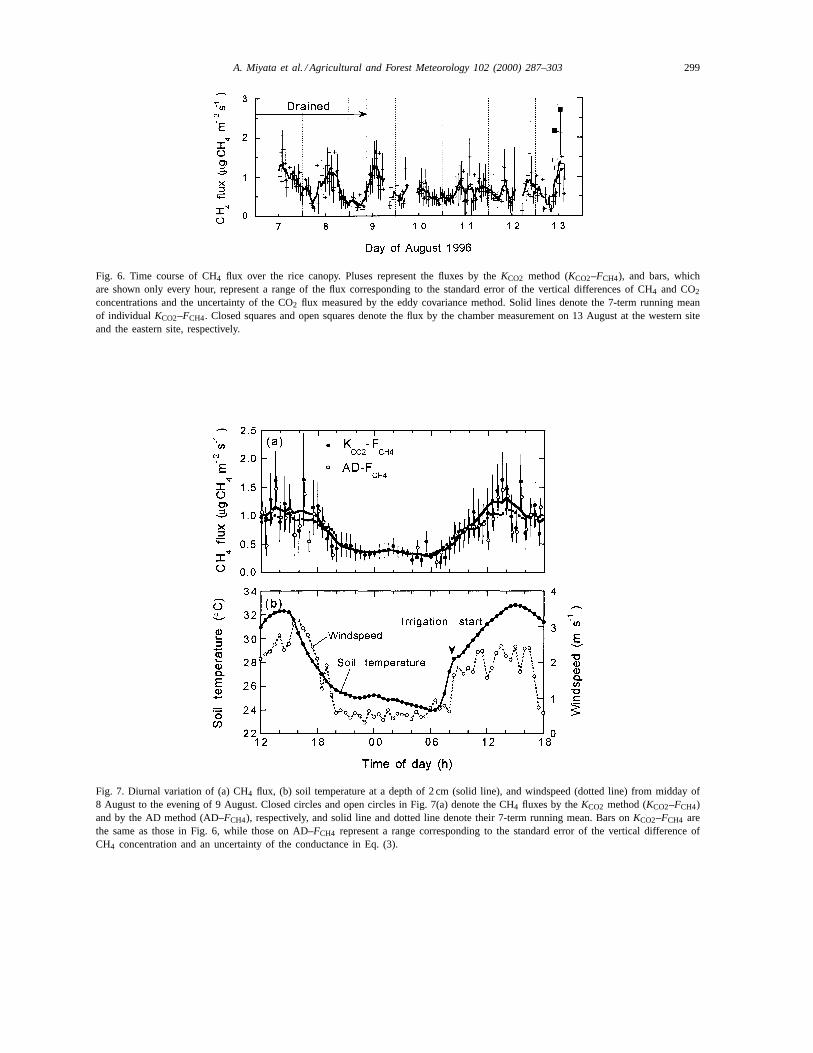
Detailed diurnal variations ofKCO2–FCH4 and theCH4 flux by the aerodynamic method (AD–FCH4)from midday of 8 August to the evening of 9 Augustare shown in Fig. 7. Also shown are the diurnal vari-ations of the soil temperature at a depth of 2 cm andthe windspeed at a height of 2.2 m. Bars on AD–FCH4represent a range corresponding to the standard errorof the vertical CH4 concentration difference and theuncertainty of conductanceD (Eq. (3)) which origi-nates mainly fromζ . Under low windspeed conditionsfound at night,u∗ and H determined by the eddycovariance method have considerable uncertainties.Sinceζ is proportional tou∗−3 (Eq. (2)), any mea-surement errors inu∗ are greatly amplified inζ . Themeasurement errors inH add further uncertainty toζ .As a result,ζ andD under low windspeed conditionswere not reliable. In fact, the estimated uncertaintyin AD–FCH4 under such conditions was one orderof magnitude greater than that inKCO2–FCH4. Forthese reasons, we excluded AD–FCH4 when u∗ was<0.1 m s−1 (this threshold was equivalent to 0.7 m s−1
in horizontal windspeed at 2.2 m) from the figure andthe following analysis. As shown in Fig. 7a, the day-time AD–FCH4 (the 7-term running mean) is a littlesmaller thanKCO2–FCH4, but the fluxes by the twomethods are generally in agreement with each otherwithin the measurement error. Fig. 7 demonstratesthat the pattern in the diurnal variation of the CH4fluxes is quite similar to those of soil temperatureand windspeed, which decrease gradually from theafternoon through the night and increase from themorning to the afternoon.
The daily budget of CH4 flux from the paddy isshown in Fig. 8. Missing flux data from 7 to 9 Augustwere interpolated using relationships between the fluxand soil temperature at a depth of 2 cm. The relation-ships were determined each day by fitting a polyno-mial function of second degree using the least squaresmethod (the fitting passed thex2-test on a significantlevel of 5%). For other days, missing data were in-terpolated using the average of each 5 data points be-fore and after the missing period. As shown again inFig. 8, the fluxes by the AD method are systematically
A. Miyata et al. / Agricultural and Forest Meteorology 102 (2000) 287–303 299
Fig. 6. Time course of CH4 flux over the rice canopy. Pluses represent the fluxes by theKCO2 method (KCO2–FCH4), and bars, whichare shown only every hour, represent a range of the flux corresponding to the standard error of the vertical differences of CH4 and CO2
concentrations and the uncertainty of the CO2 flux measured by the eddy covariance method. Solid lines denote the 7-term running meanof individual KCO2–FCH4. Closed squares and open squares denote the flux by the chamber measurement on 13 August at the western siteand the eastern site, respectively.
Fig. 7. Diurnal variation of (a) CH4 flux, (b) soil temperature at a depth of 2 cm (solid line), and windspeed (dotted line) from midday of8 August to the evening of 9 August. Closed circles and open circles in Fig. 7(a) denote the CH4 fluxes by theKCO2 method (KCO2–FCH4)and by the AD method (AD–FCH4), respectively, and solid line and dotted line denote their 7-term running mean. Bars onKCO2–FCH4 arethe same as those in Fig. 6, while those on AD–FCH4 represent a range corresponding to the standard error of the vertical difference ofCH4 concentration and an uncertainty of the conductance in Eq. (3).
300 A. Miyata et al. / Agricultural and Forest Meteorology 102 (2000) 287–303
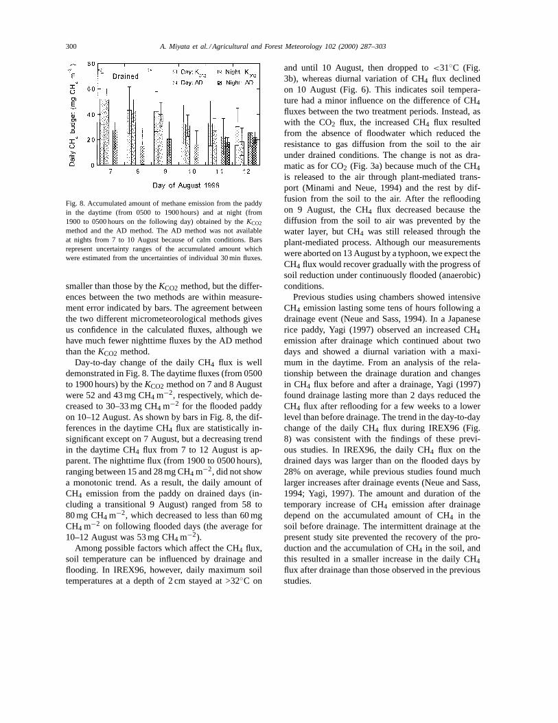
Fig. 8. Accumulated amount of methane emission from the paddyin the daytime (from 0500 to 1900 hours) and at night (from1900 to 0500 hours on the following day) obtained by theKCO2
method and the AD method. The AD method was not availableat nights from 7 to 10 August because of calm conditions. Barsrepresent uncertainty ranges of the accumulated amount whichwere estimated from the uncertainties of individual 30 min fluxes.
smaller than those by theKCO2 method, but the differ-ences between the two methods are within measure-ment error indicated by bars. The agreement betweenthe two different micrometeorological methods givesus confidence in the calculated fluxes, although wehave much fewer nighttime fluxes by the AD methodthan theKCO2 method.
Day-to-day change of the daily CH4 flux is welldemonstrated in Fig. 8. The daytime fluxes (from 0500to 1900 hours) by theKCO2 method on 7 and 8 Augustwere 52 and 43 mg CH4 m−2, respectively, which de-creased to 30–33 mg CH4 m−2 for the flooded paddyon 10–12 August. As shown by bars in Fig. 8, the dif-ferences in the daytime CH4 flux are statistically in-significant except on 7 August, but a decreasing trendin the daytime CH4 flux from 7 to 12 August is ap-parent. The nighttime flux (from 1900 to 0500 hours),ranging between 15 and 28 mg CH4 m−2, did not showa monotonic trend. As a result, the daily amount ofCH4 emission from the paddy on drained days (in-cluding a transitional 9 August) ranged from 58 to80 mg CH4 m−2, which decreased to less than 60 mgCH4 m−2 on following flooded days (the average for10–12 August was 53 mg CH4 m−2).
Among possible factors which affect the CH4 flux,soil temperature can be influenced by drainage andflooding. In IREX96, however, daily maximum soiltemperatures at a depth of 2 cm stayed at >32◦C on
and until 10 August, then dropped to<31◦C (Fig.3b), whereas diurnal variation of CH4 flux declinedon 10 August (Fig. 6). This indicates soil tempera-ture had a minor influence on the difference of CH4fluxes between the two treatment periods. Instead, aswith the CO2 flux, the increased CH4 flux resultedfrom the absence of floodwater which reduced theresistance to gas diffusion from the soil to the airunder drained conditions. The change is not as dra-matic as for CO2 (Fig. 3a) because much of the CH4is released to the air through plant-mediated trans-port (Minami and Neue, 1994) and the rest by dif-fusion from the soil to the air. After the refloodingon 9 August, the CH4 flux decreased because thediffusion from the soil to air was prevented by thewater layer, but CH4 was still released through theplant-mediated process. Although our measurementswere aborted on 13 August by a typhoon, we expect theCH4 flux would recover gradually with the progress ofsoil reduction under continuously flooded (anaerobic)conditions.
Previous studies using chambers showed intensiveCH4 emission lasting some tens of hours following adrainage event (Neue and Sass, 1994). In a Japaneserice paddy, Yagi (1997) observed an increased CH4emission after drainage which continued about twodays and showed a diurnal variation with a maxi-mum in the daytime. From an analysis of the rela-tionship between the drainage duration and changesin CH4 flux before and after a drainage, Yagi (1997)found drainage lasting more than 2 days reduced theCH4 flux after reflooding for a few weeks to a lowerlevel than before drainage. The trend in the day-to-daychange of the daily CH4 flux during IREX96 (Fig.8) was consistent with the findings of these previ-ous studies. In IREX96, the daily CH4 flux on thedrained days was larger than on the flooded days by28% on average, while previous studies found muchlarger increases after drainage events (Neue and Sass,1994; Yagi, 1997). The amount and duration of thetemporary increase of CH4 emission after drainagedepend on the accumulated amount of CH4 in thesoil before drainage. The intermittent drainage at thepresent study site prevented the recovery of the pro-duction and the accumulation of CH4 in the soil, andthis resulted in a smaller increase in the daily CH4flux after drainage than those observed in the previousstudies.
A. Miyata et al. / Agricultural and Forest Meteorology 102 (2000) 287–303 301
As mentioned earlier, the diurnal variation in theCH4 flux under drained conditions showed a distinctpositive correlation with soil temperature and wind-speed (Fig. 7). This is because temperatures up to30–35◦C accelerate CH4 production by methanogenicbacteria in the soil, and the amount of CH4 dissolvedin the soil solution decreases with increasing temper-ature (Minami and Neue, 1994). Plant-mediated CH4transport also shows an increase with increasing tem-perature (Nouchi et al., 1994; Hosono and Nouchi,1996), although the relationships found by these au-thors were between the seasonal variation of CH4 fluxand temperature rather than the diurnal variation ob-served here. As well as these temperature effects, thedistinct diurnal variation of the CH4 flux observedduring IREX96 was influenced by windspeed whichaffects the diffusion resistance from the soil to theair under drained conditions. Drainage and floodingthus affect the CH4 flux by changing the diffusionresistance to CH4 transport from the soil to air aswell as by changing the CH4 production rates in thesoil.
Methane fluxes were also measured by the closedchamber method on 13 August. The measurementswere made in the morning (0930–1100 hours) and inthe early afternoon (1215–1345 hours) at two adja-cent locations at each site, and the average of eachpair of measurements are shown in Fig. 6. The fluxesat the eastern site were 1.2 and 1.3mg CH4 m−2 s−1,while those at the western site were 2.2 and 2.7mgCH4 m−2 s−1. Measurements using the chamber atthe eastern site were comparable with the runningmean of KCO2–FCH4, but fluxes from the westernsite were double the peak observed from the mi-crometeorological measurements. It is likely thatspatial inhomogeneity caused by variation in den-sity of rice plants, nutrient status of the soil andwater depth are partly responsible for difference influxes measured by the chambers at the two sites. Inone of the few other comparisons published, Kane-masu et al. (1995) found that CH4 fluxes from ricepaddies estimated using closed chambers exceededmicrometeorological measurements by a factor of2. Further detailed studies are required to clarifywhether spatial heterogeneity is sufficient to explainsuch discrepancies or whether there are systematicmethodological differences between the measurementtechniques.
5. Conclusion
During IREX96, net CO2 and CH4 fluxes weremeasured over an intermittently drained and floodedJapanese paddy field using micrometeorologicalmethods. From the comparison of the gas fluxes un-der drained and flooded conditions we conclude: (1)The daily net uptake of CO2 from the atmosphereby the paddy field was 50% lower when the paddywas drained than when it was flooded. (2) The dailyCH4 emission on drained days was 28% larger thanon flooded days. (3) Enhanced fluxes of CO2 andCH4 from the drained soil were due to removal ofthe barrier to gas transport from the soil surface tothe air caused by the floodwater. The present studymade it clear how flooding and drainage affect theexchanges of CO2 and CH4 at rice paddies in theshort term. We need further measurements throughouta rice cultivation period to assess the long term effectof an intermittent drainage practice on the exchangesof these gases at rice paddies.
Acknowledgements
We express special thanks to the following persons.E. Ohtaki, Okayama University, for sincere supportduring IREX96; Taejin Choi, Yonsei University, andC. Drury, CSIRO, for technical support in the field;T. Miura, Okayama University, for providing us withunpublished data at IREX96; M. Tada, the managerof the Hachihama experimental farm, for use of thefacilities of the farm; E. Ishibashi, Okayama PrefectureAgricultural Experiment Station, for use of GC-FID;H. Sakai, NIAES, for providing us with rice respirationdata.
This study was supported by ‘The Bilateral Inter-national Joint Research by Special Coordination FundPromoting for Science and Technology (FY 1996)’and ‘Japanese Study on the Behavior of GreenhouseGases and Aerosols (FY 1990–1999)’ by Research andDevelopment Bureau, Japan Science and TechnologyAgency. The travel of Australian authors to Japan wassupported by the Australian Department of ScienceMultifunction Polis Program, and that of Korean au-thor was supported by Eco-Frontier Fellowship Pro-gram (FY 1996) by the Japan Environment Agency.The Korean author acknowledges support from the
302 A. Miyata et al. / Agricultural and Forest Meteorology 102 (2000) 287–303
Ministry of Agriculture and Fisheries of Korea throughthe Special Project (295133-4) for the AgriculturalTechnology Development.
References
Baker, J.T., Laugel, F., Boote, K.J., Allen Jr, L.H., 1992. Effectsof daytime carbon dioxide concentration on dark respiration inrice. Plant, Cell Environ. 15, 231–239.
Cicerone, R.J., Shetter, J.D., 1981. Sources of atmosphericmethane: measurements in rice paddies and a discussion. J.Geophys. Res. 86, 7203–7209.
Denmead, O.T., 1991. Sources and sinks of greenhouse gases inthe soil–plant environment. Vegetatio 91, 73–86.
Denmead, O.T., 1994. Measuring fluxes of greenhouse gasesbetween rice fields and the atmosphere. In: Peng, S., et al.(Eds.), Climate Change and Rice. Springer, Berlin, pp. 15–29.
Dyer, A.J., Hicks, B.B., 1970. Flux-gradient relationships in theconstant flux layer. Q. J. R. Meteorol. Soc. 96, 715–721.
Edwards, G.C., Neumann, H.H., den Hartog, G., Thurtell, G.W.,Kidd, G., 1994. Eddy correlation measurements of methanefluxes using a tunable diode laser at the Kinosheo Lake towersite during the Northern Wetlands Study (NOWES). J. Geophys.Res. 99, 1511–1517.
Fowler, D., Duyzer, J.H., 1989. Micrometeorological techniquesfor the measurement of trace gas exchange. In: Andreae,M.O., Schimel, D.S. (Eds.), Exchange of Trace Gases betweenTerrestrial Ecosystems and the Atmosphere. Wiley, Chichester,pp. 189–207.
Harazono, Y., Miyata, A., 1997. Evaluation of greenhouse gasfluxes over agricultural and natural ecosystems by means ofmicrometeorological methods. J. Agric. Meteorol. 52, 477–480.
Harazono, Y., Miyata, A., Yoshimoto, M., Mikasa, H., Oku,T., 1995. Development of a movable NDIR-methane analyzerand its application for micrometeorological measurements ofmethane flux over grasslands. J. Agric. Meteorol. 51, 27–35(in Japanese with English abstract and captions).
Harazono, Y., Monji, N., Miyata, A., Kita, K., Hamotani, K.,Uchida, Y., Yoshimoto, M., Sano, T., Fujiwara, M., Isobe,S., Ogawa, T., 1996. Development of measurement methodsfor trace gas fluxes in the surface boundary layer and abasic examination of the flux evaluation. Bull. Natl. Inst.Agro-Environ. Sci., Tsukuba, Japan 13, 166–226 (in Japanesewith English summary and captions).
Harazono, Y., Kim, J., Miyata, A., Choi, T., Yun, J.-I., Kim, J.-W.,1998. Measurement of energy budget components during theInternational Rice Experiment (IREX) in Japan. Hydrol. Process12, 2081–2092.
Hignett, P., 1992. Corrections to temperature measurements witha sonic anemometer. Boundary-Layer Meteorol. 61, 175–187.
Hirota, O., Takeda, T., 1978. Studies on utilization of solarradiation by crop stands III. Relationships between conversionefficiency of solar radiation energy and respiration ofconstruction and maintenance in rice and soybean plantpopulations. Jap. J. Crop Sci. 47, 336–343.
Holzapfel-Pschorn, A., Seiler, W., 1986. Methane emission duringa vegetation period from an Italian rice paddy. J. Geophys. Res.91, 11803–11814.
Hosono, T., Nouchi, I., 1996. Seasonal changes of methane flux andmethane concentration in soil water in rice paddies. J. Agric.Meteorol. 52, 107–115 (in Japanese with English abstract andcaptions).
Inoue, E., Tani, N., Imai, K., Isobe, S., 1958. The aerodynamicmeasurement of photosynthesis over the wheat field. J. Agric.Meteorol., 13, 121–125 (in Japanese with English abstract).
Inoue, E., Uchijima, Z., Saito, T., Isobe, S., Uemura, K., 1969. The“Assimitron”, a newly devised instrument for measuring CO2
flux in the surface air layer. J. Agric. Meteorol. 25, 165–171.IPCC, 1995. Climate Change 1995: The Science of Climate
Change. In: Houghton, J.T., Meira Filho, L.G., Callander, B.A.,Harris, N., Kattenberg, A., Maskell, K. (Eds.), Cambridge Univ.Press, Cambridge.
Jarvis, P.G., 1976. The interpretation of the variations in leaf waterpotential and stomatal conductance found in canopies in thefield. Phil. Trans. R. Soc. Lond. Ser. B-Biol. Sci. 273, 593–610.
Kaimal, J.C., Gaynor, J.E., 1991. Another look at sonicthermometry. Boundary-Layer Meteorol. 56, 401–410.
Kanemasu, E.T., Flitcroft, I.D., Shah, T.D.H., Nie, D., Thurtell,G.W., Kidd, G., Simpson, I., Lin, M., Neue, H.-U., Bronson,K., 1995. In: Peng, S., et al. (Eds.), Climate Change and Rice.Springer, Berlin, pp. 91–101.
Kelliher, F.M., Leuning, R., Schulze, E.-D., 1993. Evaporationand canopy characteristics of coniferous forests and grasslands.Oecologia 95, 153–163.
Khalil, M.A., Rasmussen, R.A., Shearer, M.J., Dalluge, R.W., Ren,L.X., Duan, C.-L., 1998. Measurements of methane emissionfrom rice fields in China. J. Geophys. Res. 103, 25181–25210.
Kim, J., Verma, S.B., Billesbach, D.P., 1998a. Seasonal variationin methane emission from a temperate Phragmites-dominatedmarsh: effect of growth stage and plant-mediated transport.Global Change Biol. 5, 433–440.
Kim, J., Verma, S.B., Billesbach, D.P., Clement, R.J., 1998b.Diel variation in methane emission from a midlatitude prairiewetland: significance of convective throughflow inPhragmitesaustralis. J. Geophys. Res. 103, 28029–28039.
Kobashi, H., Nagahori, K., Tanemura, C., Ogino, Y., 1968.Investigation of the physical and mechanical characteristics ofpoldered paddy fields in Kojima Bay. Scientific Reports on theFaculty of Agriculture, Okayama Univ. 31, 29–44 (in Japanese).
Koyama, T., 1963. Gaseous metabolism in lake sediments andpaddy soils and the production of atmospheric methane andhydrogen. J. Geophys. Res. 68, 3971–3973.
Leuning, R., 1995. A critical appraisal of combinedstomatal-photosynthesis model for C3 plants. Plant, CellEnviron. 18, 339–357.
Leuning, R., Judd, M.J., 1996. The relative merits of open- andclosed-path analysers for measurements of eddy fluxes. GlobalChange Biol. 2, 241–253.
Leuning, R., Moncrieff, J., 1990. Eddy-covariance CO2 fluxmeasurements using open- and closed-path CO2 analyzers:corrections for analyzer water vapor sensitivity and damping offluctuations in air sampling tubes. Boundary-Layer Meteorol.53, 63–76.
A. Miyata et al. / Agricultural and Forest Meteorology 102 (2000) 287–303 303
Leuning, R., Denmead, O.T., Miyata, A., Kim, J., 2000.Source/sink distributions of heat, water vapor, carbon dioxideand methane in rice canopies estimated using Lagrangiandispersion analysis, Agric. For. Meteorol., submitted.
Minami, K., Neue, H.-U., 1994. Rice paddies as a methane source.Climate Change 27, 13–26.
Monteith, J.L., Unsworth, M.H., 1990. Crop Micrometeorology.In: Principles of Environmental Physics 2nd Edition. Arnold,London, pp. 231–244.
Moore, C.J., 1986. Frequency response corrections for eddycorrelation systems. Boundary-Layer Meteorol. 37, 17–35.
Neue, H.-U., Sass, R.L., 1994. Trace gas emissions from ricefields. In: Prinn, R.G. (Ed.), Global Atmospheric–BiosphericChemistry. Plenum Press, New York, pp. 119–147.
Nouchi, I., 1994. Mechanisms of methane transport through riceplants. In: Minami, K., Mosier, A., Sass, R. (Eds.), CH4 andN2O. Global Emissions and Controls from Rice Fields andOther Agricultural and Industrial Sources. Yokendo, Tokyo,Japan, pp. 87–104.
Nouchi, I., Hosono, T., Aoki, K., Minami, K., 1994. Seasonalvariation in methane flux from rice paddies associated withmethane concentration in soil water, biomass and temperature,and its modeling. Plant and Soil 161, 195–208.
Ohtaki, E., 1984. Application of an infrared carbon dioxideand humidity instrument to studies of turbulent transport.Boundary-Layer Meteorol. 29, 85–107.
Ohtaki, E., Matsui, T., 1982. Infrared device for simultaneousmeasurement of atmospheric carbon dioxide and water vapor.Boundary-Layer Meteorol. 24, 109–119.
Philip, J.R., 1961. The theory of heat flux meters. J. Geophys.Res. 66, 571–579.
Saitoh, K., Sugimoto, M., Shimoda, H., 1998. Effects of darkrespiration on dry matter production of field grown rice stand.Comparison of growth efficiencies in 1991 and 1992. PlantProd. Sci. 1, 106–112.
Sass, R.L., Fisher, F.M., Harcombe, P.A., Turner, F.T., 1990.Methane production and emission in a Texas rice field. GlobalBiogeochem. Cycles 4, 47–68.
Schuepp, H., Leclerc, M.Y., Macpherson, J.I., Desjardins, R.L.,1990. Footprint prediction of scalar fluxes from analyticalsolutions of the diffusion equation. Boundary-Layer Meteorol.50, 355–373.
Schulze, E.-D., Leuning, R., Kelliher, F.M., 1995. Environmentalregulation of surface conductance for evaporation fromvegetation. Vegetatio 121, 79–87.
Schütz, H., Holzapfel-Pschorn, A., Conrad, R., Rennenberg, H.,Seiler, W., 1989. A 3-year continuous record on the influence ofdaytime, season, and fertilizer treatment on methane emission
rates from an Italian rice paddy. J. Geophys. Res. 94, 16405–16416.
Shurpali, N.J., Verma, S.B., Clement, R.J., Billesbach, D.P., 1993.Seasonal distribution of methane flux in a Minnesota peatlandmeasured by eddy correlation. J. Geophys. Res. 98, 20649–20655.
Simpson, I.J., Thurtell, G.W., Kidd, G.E., Lin, M.,Demetriades-Shah, T.H., Flitcroft, I.D., Kanemasu, E.T., Nie,D., Bronson, K.F., Neue, H.U., 1995. Tunable diode lasermeasurements of methane fluxes from an irrigated rice paddyfield in Philippines. J. Geophys. Res. 100, 7283–7290.
Tsukamoto, O., 1993. Turbulent fluxes over paddy field undervarious ponding depth. J. Agric. Meteorol. 49, 19–25 (inJapanese with English abstract and captions).
Tsukamoto, O., 1994. Reply to ‘Discussion on Turbulent fluxesover paddy field under various ponding depth’ by Harazono,Y. J. Agric. Meteorol. 49, 307–308 (in Japanese).
Uchijima, Z., 1961. On characteristics of heat balance of waterlayer under paddy plant cover. Bull. Natl. Inst. Agric. Sci.,Tokyo, Japan A8, 243–265.
Uchijima, Z., 1976. Maize and rice. In: Monteith, J.L. (Ed.),Vegetation and the Atmosphere Vol. 2. Academic Press,London, pp. 33–64.
Verma, S.B., Ullman, F.G., Billesbach, D., Clement, R.J., Kim,J., Verry, E.S., 1992. Eddy correlation measurements ofmethane flux in a northern peatland ecosystem. Boundary-LayerMeteorol. 58, 289–304.
Webb, E.K., 1970. Profile relationships: the log-linear range, andextension to strong stability. Q. J. R. Meteorol. Soc. 106, 85–100.
Webb, E.K., Pearman, G.I., Leuning, R., 1980. Correction of fluxmeasurements for density effects due to heat and water vaportransfer. Q. J. R. Meteorol. Soc. 106, 85–100.
Yagi, K., 1997. Methane emission from paddy fields. Bull. Natl.Inst. Agro-Environ. Sci., Tsukuba, Japan 14, 96–210.
Yagi, K., Minami, K., 1990. Effect of organic matter applicationon methane emission from some Japanese paddy fields. SoilSci. Plant Nutr. 36, 599–610.
Yagi, K., Minami, K., 1993. Spatial and temporal variations ofmethane flux from a rice paddy field. In: Oremland, R.S. (Ed.),Biogeochemistry of Global Change: Radiatively Active TraceGases. Chapman & Hall, New York, pp. 353–368.
Yamaguchi, J., Watanabe, K., Tanaka, A., 1975. Studies on thegrowth efficiency of crop plant (Part 4). Respiratory rate andthe growth efficiency of various organs of rice and maize. J.Sci. Soil Manure, Japan 46, 113–119.
Yamamoto, H., Suzuki, Y., Hayakawa, S., 1995. Estimation of leafarea index in crop canopies using plant canopy analyzer. Jap.J. Crop Sci. 64, 333–335.