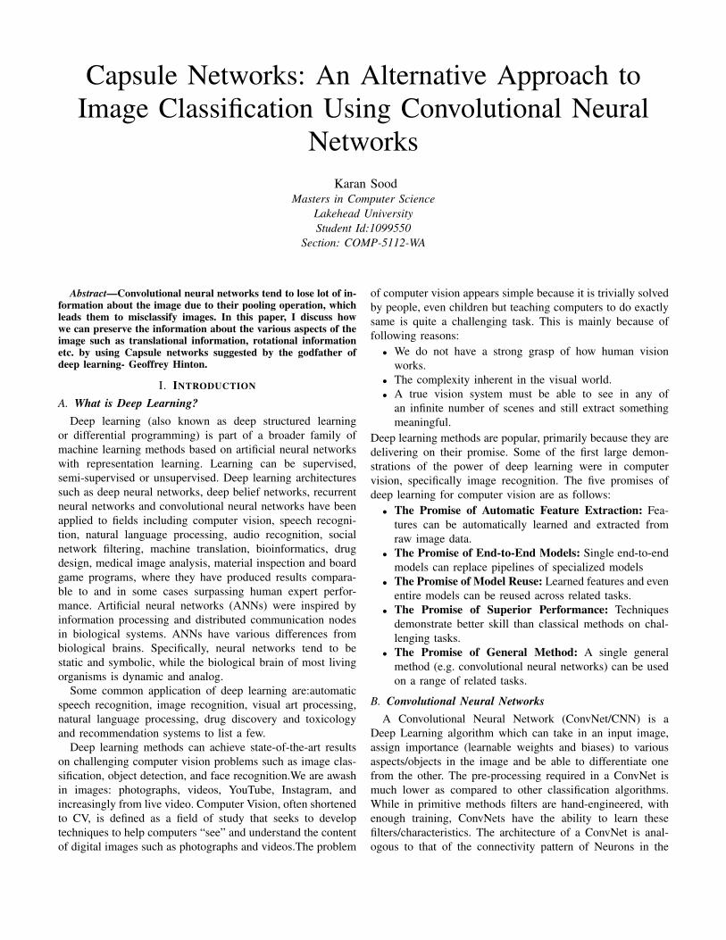
Capsule Networks: An Alternative Approach toImage Classification Using Convolutional Neural

NetworksKaran Sood

Masters in Computer ScienceLakehead UniversityStudent Id:1099550

Section: COMP-5112-WA

Abstract—Convolutional neural networks tend to lose lot of in-formation about the image due to their pooling operation, whichleads them to misclassify images. In this paper, I discuss howwe can preserve the information about the various aspects of theimage such as translational information, rotational informationetc. by using Capsule networks suggested by the godfather ofdeep learning- Geoffrey Hinton.

I. INTRODUCTION

A. What is Deep Learning?Deep learning (also known as deep structured learning

or differential programming) is part of a broader family ofmachine learning methods based on artificial neural networkswith representation learning. Learning can be supervised,semi-supervised or unsupervised. Deep learning architecturessuch as deep neural networks, deep belief networks, recurrentneural networks and convolutional neural networks have beenapplied to fields including computer vision, speech recogni-tion, natural language processing, audio recognition, socialnetwork filtering, machine translation, bioinformatics, drugdesign, medical image analysis, material inspection and boardgame programs, where they have produced results compara-ble to and in some cases surpassing human expert perfor-mance. Artificial neural networks (ANNs) were inspired byinformation processing and distributed communication nodesin biological systems. ANNs have various differences frombiological brains. Specifically, neural networks tend to bestatic and symbolic, while the biological brain of most livingorganisms is dynamic and analog.

Some common application of deep learning are:automaticspeech recognition, image recognition, visual art processing,natural language processing, drug discovery and toxicologyand recommendation systems to list a few.

Deep learning methods can achieve state-of-the-art resultson challenging computer vision problems such as image clas-sification, object detection, and face recognition.We are awashin images: photographs, videos, YouTube, Instagram, andincreasingly from live video. Computer Vision, often shortenedto CV, is defined as a field of study that seeks to developtechniques to help computers “see” and understand the contentof digital images such as photographs and videos.The problem

of computer vision appears simple because it is trivially solvedby people, even children but teaching computers to do exactlysame is quite a challenging task. This is mainly because offollowing reasons:

• We do not have a strong grasp of how human visionworks.

• The complexity inherent in the visual world.• A true vision system must be able to see in any of

an infinite number of scenes and still extract somethingmeaningful.

Deep learning methods are popular, primarily because they aredelivering on their promise. Some of the first large demon-strations of the power of deep learning were in computervision, specifically image recognition. The five promises ofdeep learning for computer vision are as follows:

• The Promise of Automatic Feature Extraction: Fea-tures can be automatically learned and extracted fromraw image data.

• The Promise of End-to-End Models: Single end-to-endmodels can replace pipelines of specialized models

• The Promise of Model Reuse: Learned features and evenentire models can be reused across related tasks.

• The Promise of Superior Performance: Techniquesdemonstrate better skill than classical methods on chal-lenging tasks.

• The Promise of General Method: A single generalmethod (e.g. convolutional neural networks) can be usedon a range of related tasks.

B. Convolutional Neural NetworksA Convolutional Neural Network (ConvNet/CNN) is a

Deep Learning algorithm which can take in an input image,assign importance (learnable weights and biases) to variousaspects/objects in the image and be able to differentiate onefrom the other. The pre-processing required in a ConvNet ismuch lower as compared to other classification algorithms.While in primitive methods filters are hand-engineered, withenough training, ConvNets have the ability to learn thesefilters/characteristics. The architecture of a ConvNet is anal-ogous to that of the connectivity pattern of Neurons in the

human brain and was inspired by the organization of theVisual Cortex. Individual neurons respond to stimuli only ina restricted region of the visual field known as the ReceptiveField. A collection of such fields overlap to cover the entirevisual area.

1) Why ConvNets over Feed-Forward Neural Nets?: Incases of extremely basic binary images, the method of usingfeed forward neural networks might show an average precisionscore while performing prediction of classes but would havelittle to no accuracy when it comes to complex imageshaving pixel dependencies throughout. A ConvNet is able tosuccessfully capture the Spatial and Temporal dependenciesin an image through the application of relevant filters. Thearchitecture performs a better fitting to the image dataset dueto the reduction in the number of parameters involved andreusability of weights. In other words, the network can betrained to understand the sophistication of the image better.

Consider the following input image: In the figure, we

Fig. 1. Input image

have an RGB image which has been separated by its threecolor planes- Red, Green, and Blue. There are a number ofsuch color spaces in which images exist — Grayscale, RGB,HSV, CMYK, etc. When an image reaches higher dimensionssuch as 8k (7680 x 4320), then it would turn out to be verycomputationally expensive if a regular feed-forward networkis used. The role of the ConvNet is to reduce the images intoa form which is easier to process, without losing featureswhich are critical for getting a good prediction. This isimportant when we are to design an architecture which is notonly good at learning features but also is scalable to massivedatasets.

2) The Convolution operation: In the figure shown below,the green section resembles our 5x5x1 input image, I. The ele-ment involved in carrying out the convolution operation in thefirst part of a Convolutional Layer is called the Kernel/Filter,K, represented in the color yellow. We have selected K as a3x3x1 matrix.

Fig. 2. Convolution operation

The Kernel shifts 9 times because of stride length = 1(non-strided), every time performing a matrix multiplicationoperation between K and the portion P of the image over whichthe kernel is hovering.

Fig. 3. Kernel slides with stride=1

The filter moves to the right with a certain stride value tillit parses the complete width. Moving on, it hops down to thebeginning (left) of the image with the same stride value andrepeats the process until the entire image is traversed.

C. The Convolution operationConvolutional networks fail to understand the relationship

between simple features in the deeper layers nearer to theinput and high level features closer to the output. To solvethis, they use max-pooling operation that maps a group ofpixels to a particular value, thus, creating high level feature

maps.But in doing so, they tend do lose a lot of information(for example, it has no information about the pose such astranslational and rotational information). Thus, mere presenceof some features in an image is enough for the CNN to classifyit into some category without taking into consideration therelative orientation of those features.Let us consider a very simple and non-technical example.Imagine a face with components such as the oval face, twoeyes, a nose and a mouth. For a CNN, a mere presence ofthese objects can be a very strong indicator to consider thatthere is a face in the image. It does not understand the spatialand relative orientational relationships.

Fig. 4. Non-equivariance in CNN

In this paper, I present my studies on a novel approachdeveloped by Geoffrey Hinton and his colleagues to overcomethe drawbacks of CNN discussed above. They called this newtype of network architecture- Capsule Networks. In additionto introducing this new network, they also developed analgorithm called Dynamic Routing in order to train thesenetworks.

II. THEORY

A. Inverse Graphics Approach

Computer graphics deals with constructing a visual imagefrom some internal hierarchical representation of geometricdata. Note that the structure of this representation needs totake into account relative positions of objects. That internalrepresentation is stored in computer’s memory as arraysof geometrical objects and matrices that represent relativepositions and orientation of these objects. Then, specialsoftware takes that representation and converts it into animage on the screen. This is called rendering. Inspired bythis idea, Hinton argues that brains, in fact, do the oppositeof rendering. He calls it inverse graphics: from visualinformation received by eyes, they deconstruct a hierarchicalrepresentation of the world around us and try to match itwith already learned patterns and relationships stored in thebrain. This is how recognition happens. And the key idea isthat representation of objects in the brain does not depend onview angle.

In order to correctly do classification and object recognition,it is important to preserve hierarchical pose relationships be-tween object parts. Capsule networks incorporate these relativerelationships between objects and it is represented numericallyas a 4D pose matrix.When these relationships are built intointernal representation of data, it becomes very easy for amodel to understand that the thing that it sees is just anotherview of something that it has seen before.

Fig. 5. Statue of liberty at different angles

Consider the image above. We can easily recognize that thisis the Statue of Liberty, even though both the images show itfrom different angles. This is because internal representationof the Statue of Liberty in our brain does not depend on theview angle. For a CNN, this task is really hard because itdoes not have this built-in understanding of 3D space, but fora CapsNet it is much easier because these relationships areexplicitly modeled. Another benefit of the capsule approachis that it is capable of learning to achieve state-of-the artperformance by only using a fraction of the data that aCNN would use. In this sense, the capsule networks workvery much like human brains as human brain requires onlyfew dozens of images to classify the images whereas CNNsrequire tens of thousands of images to achieve very goodperformance, which seems to be no better than the bruteforce approach.

B. What exactly are Capsule Networks?

In order to construct an image in a computer, we have todecide some parameters that define various objects present in

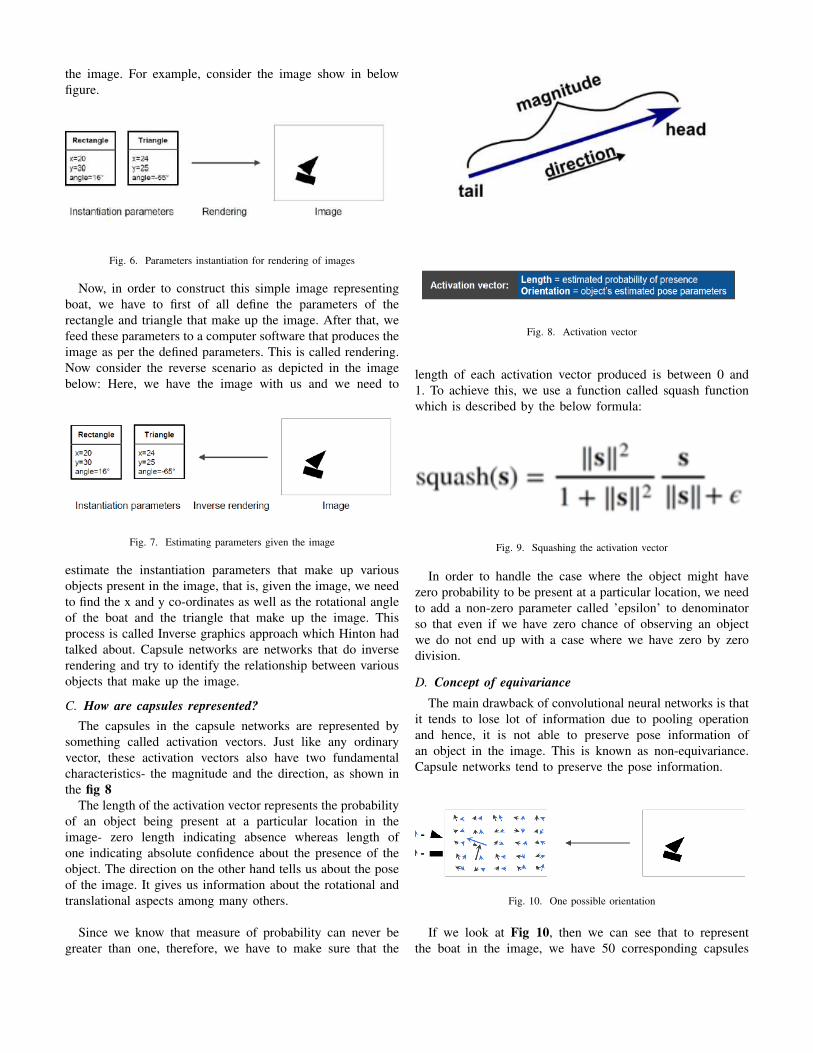
the image. For example, consider the image show in belowfigure.

Fig. 6. Parameters instantiation for rendering of images

Now, in order to construct this simple image representingboat, we have to first of all define the parameters of therectangle and triangle that make up the image. After that, wefeed these parameters to a computer software that produces theimage as per the defined parameters. This is called rendering.Now consider the reverse scenario as depicted in the imagebelow: Here, we have the image with us and we need to

Fig. 7. Estimating parameters given the image

estimate the instantiation parameters that make up variousobjects present in the image, that is, given the image, we needto find the x and y co-ordinates as well as the rotational angleof the boat and the triangle that make up the image. Thisprocess is called Inverse graphics approach which Hinton hadtalked about. Capsule networks are networks that do inverserendering and try to identify the relationship between variousobjects that make up the image.

C. How are capsules represented?The capsules in the capsule networks are represented by

something called activation vectors. Just like any ordinaryvector, these activation vectors also have two fundamentalcharacteristics- the magnitude and the direction, as shown inthe fig 8

The length of the activation vector represents the probabilityof an object being present at a particular location in theimage- zero length indicating absence whereas length ofone indicating absolute confidence about the presence of theobject. The direction on the other hand tells us about the poseof the image. It gives us information about the rotational andtranslational aspects among many others.

Since we know that measure of probability can never begreater than one, therefore, we have to make sure that the

Fig. 8. Activation vector

length of each activation vector produced is between 0 and1. To achieve this, we use a function called squash functionwhich is described by the below formula:

Fig. 9. Squashing the activation vector

In order to handle the case where the object might havezero probability to be present at a particular location, we needto add a non-zero parameter called ’epsilon’ to denominatorso that even if we have zero chance of observing an objectwe do not end up with a case where we have zero by zerodivision.

D. Concept of equivarianceThe main drawback of convolutional neural networks is that

it tends to lose lot of information due to pooling operationand hence, it is not able to preserve pose information ofan object in the image. This is known as non-equivariance.Capsule networks tend to preserve the pose information.

Fig. 10. One possible orientation

If we look at Fig 10, then we can see that to representthe boat in the image, we have 50 corresponding capsules

on the left. Among these capsules, there are two capsules oractivation vectors that have larger length as compared to othercapsules in the same figure. This represents higher probabilityof finding the triangle and rectangle at those specific positions.

Fig. 11. Changed orientation

If we look at Fig 11, then we can observe that evenon slightly changing the orientation of the boat, there is acorresponding change in the orientation of these two activationvectors as well, which demonstrates the fact that these capsulesare able to capture the pose information with the help of theactivation vectors. Thus, we can say that capsules preserve thepose information and are able to overcome the drawbacks oftraditional convolutional neural networks.

E. How do capsules work?If we consider the working of an artificial neuron, then we

can easily observe that there are three basic steps that governthe working of an artificial neuron. These are as follows:

1) Scalar product of weights: In this step, each artificialneuron receives inputs from all other neurons it isconnected to in the form of scalar values and multipliesthem with the corresponding weights to obtain scalarproducts..

2) Sum of products: In this step, all the products that havebeen calculated in the above step are added together toobtain the weighted sum of the signals that the neuronhas received.

3) Non-linear transformation: In this last step, theweighted sum obtained in the previous step is passedthrough one of the many activation functions available.This step is required to add some non-linearity tothe input so that neural network is able to capturenon-linear trends in the data as well. If we do not useany activation function, then a neural network wouldonly be able to identify the linear trends in the data andwould lead to problems such as heteroskedasticity, thatis, non-constant variance in the error terms leading tounstable confidence intervals.

A capsule has these same transformations in the vector formand an additional step where all the input vectors receivedfrom the lower level neurons are multiplied together. Thesesteps are discussed in detail below.

1) Matrix multiplication of the input vectors: Considerthree inputs from lower level capsules entering the capsule ’j’present in the layer above. The outputs from the lower levelcapsules are represented as vectors u1, u2 and u3. Lengthsof these vectors encode probabilities that lower-level capsules

detected their corresponding objects and directions of thevectors encode some internal state of the detected objects.Let us assume that lower level capsules detect eyes, nose andmouth respectively and output capsule detects face.

Fig. 12. Working of capsule

These vectors then are multiplied by corresponding weightmatrices ’W’ that encode important spatial and other rela-tionships between lower level features (eyes, mouth and nose)and higher level feature (face). For example, matrix W2j mayencode relationship between nose and face: face is centeredaround its nose, its size is 10 times the size of the nose andits orientation in space corresponds to orientation of the nose,because they all lie on the same plane. Similar intuitions canbe drawn for matrices W1j and W3j. After multiplication bythese matrices, what we get is the predicted position of thehigher level feature. In other words, u1hat represents wherethe face should be according to the detected position of theeyes, u2hat represents where the face should be according tothe detected position of the nose and u3hat represents wherethe face should be according to the detected position of themouth.If the predictions made by these three capsules point at thesame position and state of the face, then the network concludesthat it must be a face there.

2) Scalar weighting of input vectors: In artificial neuralnetworks, the neuron receiving the input signal from theneurons present in the previous layer weighs them according toweights of the corresponding neuron that connects them. Theseweights are learned by the network during back-propagation.But in case of capsule networks these weights are decided bya process called Dynamic Routing. The higher level capsulesreceive input from many lower level capsules. When the lowerlevel capsules agree on a particular prediction, they tend toform a cluster in the higher level capsule. When the outputof the lower level capsule is multiplied by the weight matrixlearned by the network, it tends to land in the cluster spaceof the higher level capsule. The lower level capsule outputwould be routed to that particular capsule where it tends toagree with predictions made by the other low-level capsules.In order to understand this better, we can consider the figuregiven below where we have two higher level capsules andone lower level capsule whose output we have to decide therouting for.

Fig. 13. Routing of input signals to capsules

In the image above, we have one lower level capsule thatneeds to “decide” to which higher level capsule it will sendits output. It will make its decision by adjusting the weightsC that will multiply this capsule’s output before sending itto either left or right higher-level capsules J and K. Now, thehigher level capsules already received many input vectors fromother lower-level capsules. All these inputs are represented byred and blue points. Where these points cluster together, thismeans that predictions of lower level capsules are close to eachother. This is why, for the sake of example, there is a clusterof red points in both capsules J and K. When we multiply thelower level capsule’s output with the weight matrix, it landsfar from the cluster of red dots in capsule J whereas for othercapsule, that is capsule K, it lands near the cluster of red dots.So, the output of the lower level capsule would be routed tocapsule K rather than capsule J.

3) Sum of the weighted input vectors: This is same asthe regular artificial neurons where we simply sum up theweighted outputs. The only difference in the capsule networksis that we have the addition of vectors here.

4) Squashing of the vectors: Just like I mentioned that thelength of the activation vector represents the probability offinding an object at a particular position in the image, it needsto be ensured that it does not exceed one as the probability cannever be greater than one. For this purpose, we make use ofsquash function that takes in a vector as an input and producesanother vector that has length between 0 and 1 and withoutany change in the original direction. This operation is knownas the squashing operation.

F. The dynamic routing between the capsules1) The calculation of actual output of target capsules:

Consider the following picture showing a simple boat madeup of a rectangle and a triangle.

In this picture, we have to route the predicted output fromthe lower level capsules to the higher layer which contains twocapsules because there are two possibilities for the object-oneis the object being a house and the other one is the object

Fig. 14. Routing mechanism

being a boat. In order to decide the path, the following stepsare followed:

• Initializing the raw routing weights to zero: In thisstep, all the weights are initialized to zero. These areknown as the raw routing weights represented as bj .

• Calculating the actual routing weights: The second stepis to apply soft-max activation function to the raw routingweights calculated in the previous step to obtain the actualrouting weights that are represented as cj .

• Weighted sum calculation: In this step, the routingweights obtained in the previous step are multipliedby the predicted output. In doing so, it might happenthat the length of the vectors become greater than one,therefore, we need to apply squash function one moretime to satisfy the probability constraint. This gives usthe calculated actual output of the higher level capsuleswhich is represented as vj .

Fig. 15. Actual output calculation

The figure above shows how the actual output is calculatedusing the routing mechanism.

After calculating the actual output, we need to update therouting weights to make our model learn. In order to update therouting weights, we first of all calculate the degree of similaritybetween the predicted output and the actual output. This isdone by calculating the dot product of the predicted vector andthe calculated vector. When there is agreement, that is anglebetween the two vectors is less than 90 degrees, its cosinevalue is positive and there is a corresponding increase in therouting weight. On the other hand, when the angle between the

two vectors is greater than 90 degrees, then cosine of that anglebecomes negative resulting in decrease in the correspondingrouting weights. In below figure, there is similarity betweenthe predicted and the actual output and hence, there is anincrease in the routing weights.

Fig. 16. Routing weights increase

The dissimilarity between the predicted output and theactual output causes the routing weights to decrease as shownin the figure below.

Fig. 17. Routing weights decrease

2) Convergence of the algorithm: This whole processdescribed above is just a single iteration in dynamic routingmechanism. It repeats itself over a couple of times till thereis no change in the routing weights for specified number ofiterations or else the maximum number of iterations has beenreached, whichever happens earlier.The dynamic routing, thus, helps us in preventing noise in thesystem by properly routing the outputs of lower level capsulesto appropriate capsules in the higher layer.

III. METHODOLOGY

I have used TensorFlow to implement the capsule network.

A. Feeding the input images

My first step was to create tensor flow placeholder thatwould directly feed the input images of dimensions (28 x28 x 1) to the network. Since I am working with gray-scaleimages, therefore, the last channel has the value 1. If therewere coloured images, then, the last channel value would havebeen 3 corresponding to the red, green and blue channels.

B. Building the primary layerThe second step was to build the primary capsule layer

that would try to identify different types of information aboutthe objects present in the scene. For this purpose, I used twoconvolutional layers. To the first convolutional layer, I directlyfed the input images. The output of this convolutional layerwas fed as an input to the second convolutional layer thatwas configured to output 256 feature maps with each of themcontaining 36 scalars. The feature maps were reshaped so thatI now had 32 maps containing 6 by 6 grid of 8 dimensionalvectors. This is illustrated in the image below.

Fig. 18. Convolutional feature maps reshaped

C. Modifying the squash functionThe squash function that I defined in Fig 9 has a small

problem when I tried implementing it in the TensorFlow. Theproblem is that if any of the vectors in the equation representedby Fig 9 become zero, that is when we have zero chance ofobserving an object in the given scene, then the gradients cannot be computed and the ’norm’ function of TensorFlow givesus ’NaN’ values due to which the network literally becomesdead. In order to solve this problem, the squash function canbe modified as shown in Fig 19.

Fig. 19. Modified squash function to handle NaN values

D. Implementing the digit capsulesSince there were ten classes to be identified (numbers 0 to

9), therefore, there were 10 capsules in the output layer. Eachof these capsules were 16-dimensional vectors that containedfull pose information (such as the skewness, rotation relativeto the axis etc.) of the objects present in the image to beclassified. Now, I needed to compute the output of the digitcapsules. This can be done in two steps.

1) Making predictions for the digit capsules: The firststep was to predict the output for each of the capsulespresent in the digit capsule layer. The prediction is madeby computing the product of transformation matrix learnedduring the training process and the output of the primarylevel capsules. The transformation matrix learns the part-wholerelationship between the objects present in the image and theimage itself. This process is repeated for every pair possiblebetween the lower level capsules and the number of capsulespresent in the higher layer. For example, here in the lowerlayer, there are (32 x 36 = 1152) capsules present. Therefore,there would be these many predictions for every digit capsulein the higher layer. Since there are 10 digit capsules in total,therefore, we have total of 11520 predictions. This is shownin the figure below.

Fig. 20. Predicted output for the higher-level capsules

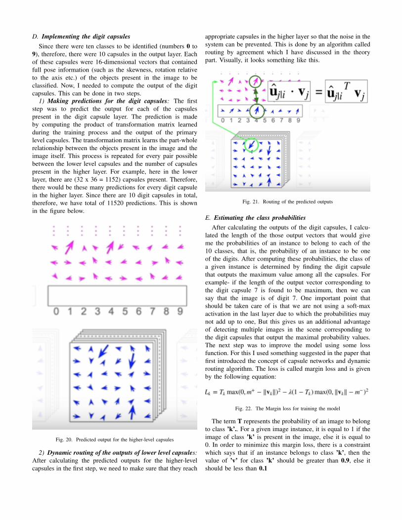
2) Dynamic routing of the outputs of lower level capsules:After calculating the predicted outputs for the higher-levelcapsules in the first step, we need to make sure that they reach

appropriate capsules in the higher layer so that the noise in thesystem can be prevented. This is done by an algorithm calledrouting by agreement which I have discussed in the theorypart. Visually, it looks something like this.

Fig. 21. Routing of the predicted outputs

E. Estimating the class probabilitiesAfter calculating the outputs of the digit capsules, I calcu-

lated the length of the those output vectors that would giveme the probabilities of an instance to belong to each of the10 classes, that is, the probability of an instance to be oneof the digits. After computing these probabilities, the class ofa given instance is determined by finding the digit capsulethat outputs the maximum value among all the capsules. Forexample- if the length of the output vector corresponding tothe digit capsule 7 is found to be maximum, then we cansay that the image is of digit 7. One important point thatshould be taken care of is that we are not using a soft-maxactivation in the last layer due to which the probabilities maynot add up to one, But this gives us an additional advantageof detecting multiple images in the scene corresponding tothe digit capsules that output the maximal probability values.The next step was to improve the model using some lossfunction. For this I used something suggested in the paper thatfirst introduced the concept of capsule networks and dynamicrouting algorithm. The loss is called margin loss and is givenby the following equation:

Fig. 22. The Margin loss for training the model

The term T represents the probability of an image to belongto class ’k’.. For a given image instance, it is equal to 1 if theimage of class ’k’ is present in the image, else it is equal to0. In order to minimize this margin loss, there is a constraintwhich says that if an instance belongs to class ’k’, then thevalue of ’v’ for class ’k’ should be greater than 0.9, else itshould be less than 0.1

The whole process up till now can be visualized as follows:

Fig. 23. A snapshot of the process

F. Computing reconstruction loss

To compute the reconstruction loss, I had to first constructthe image from the information that the network has learnt.I used a decoder for this purpose. The decoder has threefully connected layers also called dense layers with first layerhaving 512 hidden neurons, the second layer having 1024hidden units and the final one having 784 hidden units. Thedecoder produced a 784-dimensional vector containing thepixel intensity values for each 28 by 28 image instance thatwas fed to the capsule network. The reconstruction loss wascomputed by squaring the difference between the originalimage and reconstructed image. Since the original image haddimensions (28x28x1), therefore, it had to be first convertedinto 784-dimensional vector. The total loss was obtained byadding together the margin loss and the reconstruction lossbut it was scaled down in a manner to let the margin lossdominate the training process of the model. I used ”Adam”optimizer with default settings to optimize the training process.One important thing suggested in the paper was that instead ofsending all the outputs of the capsule network to the decodernetwork, we must send only the output vector of the capsulethat corresponds to the target digit. This was done by settingzeros for all the values of the digit capsules except for theone that actually represented the image. For testing instances,since labels are not known beforehand, the predictions for aparticular class was used to decide the mask.The entire process of training from the instance an input image

is fed to the network till the model fits to the data can bevisualized with the help of the following figure:

Fig. 24. The training process

The above image demonstrates the predictions made by themodel when it is dealing with the training instances. Here,the class labels are used to create the mask. When the modelhas to deal with the testing instances where the labels are notknown, the mask is created by using the predictions of themodel. This is illustrated in the figure below.

Fig. 25. The entire testing process

IV. RESULTS

A. Training accuracyI used MNIST dataset for training the model. It contained

60000 training images and 10000 test images. I did not dohyper-parameter tuning or used any dropout layer. I just trainedthe model for a few epochs, each time measuring the accuracyon the validation set and saving the model if the validation losshappened to be lowest so far. This is method is generally called’Early stopping’. The validation set contained 5000 imagesand the model computed the mean accuracy and mean lossvalue at the end of each epoch. Since TensorFlow has beenused to implement the code, GPUs or even better TPUs (tensor

processing units) can greatly enhance the speed of training andthe corresponding time would be greatly reduced. After a fewepochs, there was considerable learning by the model and itwas giving an accuracy of 99 percent on the validation setcontaining 5000 images. This is shown in the below figure:

Fig. 26. Training epochs

B. Testing accuracyAfter training the model for a few epochs, I evaluated

the model on the test set that contained 10000 images as isprovided by the creators of MNIST dataset. The test accuracyof the model was found to be 99.5 percent. Earlier, I foundit a little strange having obtained better accuracy on the testset than the training set. But, I researched and I found thatsometimes model is indeed able to better chase the errors inthe test set depending on how we split the data. The accuracyon the test set is shown in the figure below.

Fig. 27. Accuracy on the test set

C. PredictionsAfter training my model, I decided to make some pre-

dictions to have a better idea about how my model wasperforming. The model’s ability in making predictions on newdata is shown in Fig 28 and Fig 29 on the right hand side.

V. SUMMARY

The traditional use of convolutional neural networks canbe useful to some extent when we want to just label theimages and do not care much about the features that makeup the image. But, when it comes to tasks such as objectdetection or image segmentation, then convolutional nets tendto fail miserably due to loss of information during the poolingoperation that reduces the dimensionality of the feature mapscreated during the convolution operation. Thus, we can say thatconvolutional networks are non-equivariant in nature. Thisdrawback can be overcome by the use of capsule networkssuggested by Geoffrey Hinton. The capsule networks makeuse of capsules which are nothing but the activation vectorswhose length represent the probability of presence of an objectin the image and the direction represent the orientation. De-pending upon the number of dimensions used to represent theactivation vector, we can capture lot of pose information such

Fig. 28. Predictions-1

Fig. 29. Predictions-2

as translational information, rotational information, skewness,thickness of the image etc. Whenever there is even a minutechange in the image, there is a corresponding change in thevalues of the activation vector as well. This way the poseinformation of the image is preserved and we say that capsulenetworks are equivariant in nature.

VI. FUTURE WORK

There is lot of scope for improvement in the design ofthe capsule networks. Although the capsule networks havebeen able to achieve remarkable performance on the MNISTdataset, but the performance is relatively average as far as theother datasets such as CIFAR10 or CIFAR100 are concerned.We also do not have any idea about the performance of capsulenetworks on large image datasets such as ImageNet. Anotherarea that needs improvement is the dynamic routing of thecapsule networks as they significantly increase the training

time of the network, One last thing that I would like to mentionis that capsule networks are not able to detect identical objectsclose to each other. But, this may or may not be a problem aseven human eyes are not very good at it.

REFERENCES

[1] Geoffrey E.Hinton, Google Brain, Toronto, Sara Sabour, Nicholas Frost,Dynamic Routing Between Capsules, NIPS 2017.

[2] G. E. Hinton, A. Krizhevsky S. D. Wang, Transforming Auto-encoders,2011.

[3] Wei Zhao, Min Yang, Shenzen Institutes of Advanced Technology,Chinese Academy of Sciences, Jiambo Ye, Pennsylvania State Univer-sity, Zeyang Lei, Graduate School at Shenzhen, Tsinghua University,Soufei Zhang, Nanjing University of Posts and Telecommunications,Zhou Zhao, Zhejiang University, Investigating Capsule Networks withDynamic Routing for Text Classification, 2018.

[4] Mercedes E. Paoletti, Student Member, IEEE, Juan M. Haut, StudentMember, IEEE, Ruben, Fernandez-Beltran, Javier Plaza, Senior Member,IEEE, Antonio Plaza, Fellow, IEEE, and Filiberto Pla.

[5] Ningyu Zhang, Artificial Intelligence Research Institute, Zhejiang Lab,China, Shumin Deng, College of Computer Science and Technology,Zhejiang University, China, Alibaba-Zhejiang University Frontier Tech-nology Research Center, China, Zhanlin Sun, College of ComputerScience and Technology, Zhejiang University, China, Xi Chen, Collegeof Computer Science and Technology, Zhejiang University, China, WeiZhang, Alibaba-Zhejiang University Frontier Technology Research Cen-ter, China, Alibaba Group, China, Huajun Chen, College of ComputerScience and Technology, Zhejiang University, China.

[6] Steve Lawrence, Member, IEEE, C. Lee Giles, Senior Member, IEEE,Ah Chung Tsoi, Senior Member, IEEE, Andrew D. Back, Member,IEEE, Face Recognition: A Convolutional Neural-Network Approach,IEEE TRANSACTIONS ON NEURAL NETWORKS, VOL. 8, NO. 1,JANUARY 1997.

[7] Patrice Y. Simard, Dave Steinkraus, John C. Platt, Microsoft Research,One Microsoft Way, Redmond WA 98052, Best Practices for Convolu-tional Neural Networks Applied to Visual Document Analysis.

[8] Alex Krizhevsky, University of Toronto, Ilya Sutskever, University ofToronto, Geoffrey E. Hinton, University of Toronto, ImageNet Classifi-cation with Deep Convolutional Neural Networks.

[9] Tianjun Xiao, Institute of Computer Science and Technology, PekingUniversity, Yichong Xu, 2Microsoft Research, Beijing, Kuiyuan Yang,Microsoft Research, Beijing, Jiaxing Zhang, Microsoft Research, Bei-jing, Yuxin Peng, Institute of Computer Science and Technology, PekingUniversity, Zheng Zhang, Institute of Computer Science and Technology,Peking University, The Application of Two-level Attention Models inDeep Convolutional Neural Network for Fine-grained Image Classifica-tion.

[10] Dumitru Erhan, Christian Szegedy, Alexander Toshev, and DragomirAnguelov, Google, Inc, 1600 Amphitheatre Parkway, Mountain View(CA), 94043, USA.

[11] Wanli Ouyang, Ping Luo, Xingyu Zeng, Shi Qiu, Yonglong Tian,Bhuvana Ramabhadran1Hongsheng Li, Shuo Yang, Zhe Wang, YuanjunXiong, Chen Qian, Zhenyao Zhu, Ruohui Wang, Chen-Change Loy,Xiaogang Wang, Xiaoou Tang, the Chinese University of Hong Kong,DeepID-Net: multi-stage and deformable deep convolutional neuralnetworks for object detection.

[12] Jifeng Dai, Microsoft Research, Yi Li, Tsinghua University, KaimingHe, Microsoft Research, Jian Sun, Microsoft Research, R-FCN: ObjectDetection via Region-based Fully Convolutional Networks.

[13] K. Mikolajczyk, B. Leibe, and B. Schiele. Multiple object class detectionwith a generative model. In CVPR, volume 1, pages 26–36. IEEE, 2006.

[14] Tara N. Sainath, IBM T. J. Watson Research Center, Yorktown Heights,NY 10598, U.S.A, Abdel-rahman Mohamed, Department of ComputerScience, University of Toronto, Canada, Brian Kingsbury, IBM T. J.Watson Research Center, Yorktown Heights, NY 10598, U.S.A, BhuvanaRamabhadran1, IBM T. J. Watson Research Center, Yorktown Heights,NY 10598, U.S.A, DEEP CONVOLUTIONAL NEURAL NETWORKSFOR LVCSR.

[15] Amara Dinesh Kumar, R.Karthika , Latha Parameswaran , Departmentof Electronics and Communication Engineering , Amrita School ofEngineering, Coimbatore , Amrita Vishwa Vidyapeetham,India.

[16] Johannes Stallkamp, Marc Schlipsing, Jan Salmen, and Christian Igel.The german traffic sign recognition benchmark: a multi-class classifica-tion competition. In Neural Networks (IJCNN), The 2011 InternationalJoint Conference on, pages 1453–1460. IEEE, 2011.