Bank of Canada staff working papers provide a forum for staff to publish work-in-progress research independently from the Bank’s Governing Council. This research may support or challenge prevailing policy orthodoxy. Therefore, the views expressed in this paper are solely those of the authors and may differ from official Bank of Canada views. No responsibility for them should be attributed to the Bank.

www.bank-banque-canada.ca

Staff Working Paper/Document de travail du personnel 2016-12

Capital Structure, Pay Structure and Job Termination

by Jason Allen and James R. Thompson

2

Bank of Canada Staff Working Paper 2016-12

March 2016

Capital Structure, Pay Structure and Job Termination

by

Jason Allen1 and James R. Thompson2

1Financial Stability Department Bank of Canada

Ottawa, Ontario, Canada K1A 0G9 jallen@bankofcanada.ca

2University of Waterloo james@uwaterloo.ca

ISSN 1701-9397 © 2016 Bank of Canada

ii

Acknowledgements

We thank seminar participants at Queen’s University and the SFA (2015) for helpful comments. We are extremely grateful to, without implicating, Nellie Gomes and Louis Piergeti at IIROC. We thank Reint Gropp, David Martinez-Miera, Ned Prescott (discussant), Josef Schroth, Jia Xie and Jano Zabojnik for comments. We also thank Andrew Usher for excellent research assistance.

iii

Abstract

We develop a model to analyze the link between financial leverage, worker pay structure and the risk of job termination. Contrary to the conventional view, we show that even in the absence of any agency problem among workers, variable pay can be optimal despite workers being risk averse and firms risk neutral. We find that firms employing workers with safer projects (and lower probability of job termination) use more variable compensation, and that leverage is strictly increasing in the amount of variable pay. These two results lead to the main insight of the paper: the more likely it is that a worker is terminated, the lower a firm’s leverage. We provide empirical support for these predictions with a novel data set of all Canadian financial brokers and dealers. In the context of our empirical analysis, the model provides a novel mechanism to help explain why high leverage and high amounts of variable pay may be pervasive in financial relative to non-financial institutions.

JEL classification: G24, J33 Bank classification: Financial institutions; Labour markets

Résumé

Les auteurs élaborent un modèle permettant d’analyser les liens entre le levier financier, la structure de rémunération et le risque de licenciement. Contrairement à ce qui est généralement admis, ils montrent que, même en l’absence de problème de délégation entre les travailleurs et l’entreprise, une rémunération variable peut être optimale bien que les travailleurs soient réfractaires au risque et que l’entreprise soit neutre à cet égard. Les auteurs constatent que, dans les entreprises où les travailleurs sont employés à des projets plus sûrs (et où la probabilité de licenciement est plus faible), la part de la rémunération variable est plus élevée et le levier financier de l’entreprise augmente parallèlement à cette part. De ces deux constatations ressort le principal résultat de l’étude : plus la probabilité de licenciement est élevée, moins la firme est endettée. Les auteurs présentent une justification empirique de cette prévision à l’aide d’une série inédite de données portant sur l’ensemble des courtiers et négociateurs canadiens en valeurs mobilières. Dans le contexte de leur analyse empirique, le modèle qu’ils proposent offre un nouveau mécanisme expliquant pourquoi un levier financier élevé et une proportion élevée de rémunération variable sont plus répandus chez les sociétés financières que chez leurs homologues non financières.

Classification JEL : G24, J33 Classification de la Banque : Institutions financières; Marchés du travail

Non-Technical Summary

This paper develops a theoretical model to analyze the links among financial leverage,

pay structure, and job turnover. Using the model, one can rationalize why high leverage and

high amounts of variable pay are pervasive in financial relative to non-financial institutions.

The main insight of the model is that the more likely worker turnover is, the lower a firm

must keep its leverage.

Understanding the relationship among financial leverage, operating leverage, and turnover

is crucial for firms since turnover is costly as are deviations from optimal leverage. Our re-

search can better inform firms as to the benefit of using pay structure to create flexibility so

as to potentially avoid costly turnover. Furthermore, we show how pay structure can allow

for an increase in financial leverage without increasing total firm risk.

The model has three main testable implications. First, variable pay as a fraction of total

compensation decreases with the probability of job termination. Second, debt is negatively

correlated with the amount of fixed pay and positively correlated with the amount of variable

pay relative to fixed pay. Third – the main result of the paper – the higher the probability

of job termination, the less debt a firm will employ. We empirically test each of these impli-

cations using balance-sheet and income-statement data on the universe of Canadian brokers

and dealers from 1992 to 2010. Our empirical results support all three model implications.

We therefore uncover a new justification for why banks may be highly levered, and why their

wage structure may be more skewed toward variable pay relative to non-financial institu-

tions. What drives both of these results is the fact that banks tend to have lower costs of

debt, and lower costs to workers of termination.

2

1 Introduction

When a worker is risk averse and has a project that is risky, how should a risk-neutral

firm pay them? When there is an agency problem, i.e., hidden information or action related

to the worker, variable pay can be used to help correct the inefficiency. In the absence of

such problems, standard economic theory says that the worker should be paid with fixed

pay. In this paper, we re-visit this problem and show that, when the firm’s capital structure

problem is incorporated, variable pay can arise endogenously, even in the absence of agency

problems. We find supporting evidence for our model with a novel data set comprised of

all Canadian financial brokers and dealers. Financial institutions offer a particularly useful

environment in which to study the implications of our model: we are able to shed new light

on why banks may choose high levels of leverage and why they rely heavily on variable pay.

The intuition behind our theoretical results is as follows. Consider workers with risky

projects that can either have a high or low return but with no capital for implementation.

A firm contracts with workers who have the same project risk and can pay them a variable

wage, which is paid only if the return is high, and a fixed wage regardless of the return.

Although job termination is endogenous in the model, it is simplest to convey the intuition

by assuming that workers are terminated if the return is low; the worker incurs a cost of

this termination. In this environment, it is clearly optimal to pay workers with fixed pay

since they are risk averse and the firm is risk neutral. The reason is that fixed pay can

hedge the low state in which the worker is terminated. Risk aversion implies that the worker

receives more utility from fixed wages and therefore the firm minimizes its wage bill by

paying through this method.

Now consider a firm that needs to raise money for the projects and does so through

debt and equity. Assuming that debt is subsidized relative to equity, in the presence of

bankruptcy costs, the firm opts to take on as much debt as possible while avoiding the

possibility of bankruptcy in the low state. Fixed pay now works against debt, since it is

itself a form of debt on the operation side of the firm. In choosing the amount of fixed pay

to offer to workers, the firm trades off the benefit (decreased wage bill from fixed pay due to

worker risk aversion) versus the cost (having to reduce debt to avoid the bankruptcy costs).

Firms with safer projects (workers), where safer means projects have a higher probability

of success, will pay workers with more variable pay. This occurs because the value of fixed

pay, in utility terms, is lower for these types of workers, since it is less likely that they are

terminated. Thus, our model predicts that firms with safer projects will have more variable

pay and higher financial leverage. We uncover these predictions in the data.

We then use the model in the context of banks, which tend to have lower costs of debt

1

(Allen et al. (2014)) and lower costs to bankers of being terminated relative to non-financial

institutions (Jacobson et al. (1994)). When debt is cheaper, firms have an incentive to

use more of it and do so by increasing the amount of variable pay. When the cost of job

termination is low, firms use more variable pay since the benefit of fixed pay, in utility terms,

is less. This in turn allows firms to take on more debt. These then combine to support two

key features of banks that we observe in the real world: high variable pay1 and high leverage.2

Our work is related to research on the relationship between wage structure and capital

structure. Jaggia and Thakor (1994) theoretically explore the relationship between firm-

specific human capital and capital structure. Managers choose to exert less effort into firm-

specific human capital if their firm has a high probability of going bankrupt. This incentivizes

the firm to take on less debt when they value human capital. In contrast, we uncover

a relationship between the risk that a worker takes on and capital structure without any

agency problem. Thanassoulis (2012) argues that wage structure has important implications

for the probability of financial distress. A firm (bank in the context of that paper) prefers

to use variable wages to share risk with workers; however, an externality is created because

of competition among banks for bankers.3 The essence of the risk-sharing incentive in that

paper is present in our paper; however, we model heterogenous workers and explicitly consider

the capital structure problem. As such, we are able to obtain predictions on what types of

firms should have more/less variable wages and higher/lower leverage.

Empirically, Simintzi et al. (2014) provide cross-country evidence that employment pro-

tection crowds out financial leverage. The authors hypothesize that higher employment

protection increases the costs of financial distress and so debt becomes costlier. Bae et al.

(2010) find that firms with “friendlier” policies toward their employees also have less debt.

The reason is to reduce leverage risk.4 Interestingly, we show that those firms where workers

experience higher turnover actually have higher leverage. It is through the compensation

channel that operating leverage, i.e., the flexibility of operating expenses to firm conditions,

affects capital structure.

Our work is also related to the literature on worker compensation and pay-for-performance,

which has largely focused on the role of workers and an agency environment to explain the

1Lemieux et al. (2009) and Celerier and Vallee (2015) show that, on average, financial institutions pay65% of a worker’s salary as variable compensation (data from U.S. and France). This compares with 33-41%in non-financial firms (see Lemieux et al. (2009) and Celerier and Vallee (2015)).

2A typical debt-to-assets ratio for non-financial corporations is around 20%-30%, whereas for financialinstitutions it is closer to 87%-95% (Gornall and Strebulaev (2014)).

3Berk, Stanton, and Zechner (2010) argue that fixed wages that are subject to change at the firm’sdiscretion could also avoid bankruptcy.

4In contrast, in models by Bronars and Deere (1991), Dasgupta and Sengupta (1993), and Perotti andSpier (1993), high leverage is used to mitigate operational risk by limiting the bargaining power of workers.

2

use of variable pay, where fixed pay is often used to offset risk that a worker faces. Early

examples include Jensen and Meckling (1976) and Holmstrom (1979) who focus on compen-

sation and agency costs in explaining risk taking. See Lazear and Oyer (2012) for a summary

of the current literature. The empirical evidence is mixed on the trade-off between risk and

incentives implied by the standard agency model (Prendergast 1999; Prendergast 2000).

Recently, papers have begun to examine other mechanisms to help explain the prevalence

of incentive-based pay. Oyer (2004) constructs a model in which variable pay is used to avoid

costly compensation renegotiations. If the outside option of a worker is dependent on firm

value, then stock options can prevent a worker from leaving (which is costly to the firm)

without the need for renegotiation. In contrast, in our model, the worker is replaceable and

so the interim participation constraint does not imply variable wages. Instead, variable pay

arises from the firms capital structure problem and not from the worker’s problem. Bertrand

and Mullainathan (2001) and Gopalan et al. (2010) rationalize CEO pay-for-luck (wherein

CEOs are rewarded for sectoral performance and not relative performance) with a skimming

model, and with a model in which a CEO needs to choose the degree of correlation that the

firm will have with its sector. Again, these papers justify variable pay through a problem

related to the worker (a manager in these cases), whereas we show that variable pay can exist

solely because of the firm’s capital structure decision. It is important to note that although

we will not model any agency problems, this is not meant to downplay the potential role of

agency costs and incentive pay but rather to better illuminate the mechanism behind our

results.

What further sets our theory apart is that we model potential compensation not just

for management but all workers. Much of the corporate finance literature on incentives

and pay explores management compensation. One reason for this is that data on senior

management are more widely available and the effects of CEO compensation and incentives

are seemingly easier to disentangle. It is impossible to do justice to this literature; however,

three prominent examples include Jensen and Murphy (1990), Hall and Liebman (1998), and

Milbourn (2003).

Our empirical work drives the above point further since we have data on non-management

workers (in our case, within the Canadian banking industry). Although the popular press

focuses on the impressive wages of Russell 3000 executives, which within the broker-dealer

category in 2014 was an average of over $8 million per year, the typical chief executive in 2014

at a broker-dealer firm earned $238,740 in wages (Bureau of Labor Statistics occupational

employment statistics NAICS 523100). For the sample of Canadian broker-dealers, the

average wage of chief executives in 2014 was Can$300,828 (approximately US$270,745).

However, the total wage bill (including cash bonuses) for specialists and analysts is far larger

3

than for executives. Staying in Canada, on average, a specialist earns Can$131,720 and an

analyst Can$142,534 per year. In 2014, there were 16,795 specialists and 1,930 analysts

compared with 785 top executives. Thus, by focusing only on management wages, much of

the literature misses the majority of wages in an organization. This paper will hopefully

contribute to a better understanding of variable wages to all workers.

Although our theoretical contribution is general, we present a case study where we ex-

amine the financial structure and wage structure of Canadian financial institutions. This is

because we have access to detailed firm-level information on the decomposition of wages into

their fixed and variable components for these firms. In addition, we have detailed informa-

tion on financial institutions’ balance sheets and income statements. Secondly, our model

provides additional theoretic insights into financial institutions’ behavior that we discussed

above; thus the application to financial institutions seems fruitful.

The remainder of the paper is as follows. Section 2 presents the model of workers and

firms, Section 3 provides the main comparative statics, and Section 4 presents the application

of the model to financial institutions. In Section 5 we present the data, while Section 6

presents the empirical tests of the model. Section 7 contains an extension of the baseline

model that allows for bankruptcy in equilibrium, and finally, Section 8 concludes.

2 Model

In this section, we first outline the worker’s problem and then solve the firm problem.

The model has three key empirical predictions that we test in Section 6.

2.1 Worker Problem

The model is in three periods indexed t = 0, 1, 2. We assume that a worker can neither

save nor borrow and derives lifetime utility U from periods 1 and 2, which is given by the

exponential function

U = −2∑t=1

exp(−αCt), (1)

where Ct is consumption in period t and α is the coefficient of absolute risk aversion. Note

that we assume for simplicity that utility is additively separable over time and stationary.

Without loss of generality (see Section 3.1), we assume that workers do not discount utility

over the three periods.

4

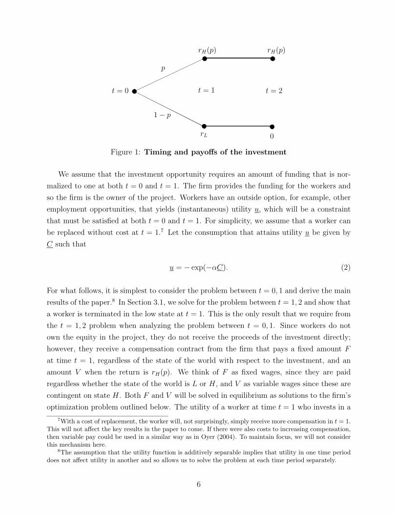
A worker is penniless but can implement an investment opportunity/project that has a

rate of return at t = 1 of rH(p) with independent and identically distributed (iid) probability

p and rL with probability 1 − p, where rH(p) > rL. A worker’s decision is simple: either

engage in the project or take an outside option to be discussed below. We will compare

firms that hire workers with different projects. The projects differ in their probability of

being in the high state. To this end, let there be a measure 1 of workers that are uniformly

distributed along the continuum of project risk level p, hence, uniformly distributed on [0, 1].

Thus, for a given risk level p, there is a continuum of workers with the same iid probabil-

ity of achieving the high return. Given that workers can differ by project risk, it seems

reasonable that the return in the high state be a function of project riskiness. We could

make the intuitive assumption that r′H(p) < 0, so that safer projects have a lower expected

return; however, neither this assumption, nor any assumption on the second derivative, is

required to obtain our results. When we analyze the capital structure choice of the firm, it

will become clear that the return in the low state plays a role. We could allow firms to differ

in this return; however, this would obfuscate the capital structure problem without offering

interesting insights into the problem that we consider. We assume that, if the high state

occurs, the investment returns rH(p) at t = 2 as it did at t = 1. If the low state occurs,

then we assume that the investment returns nothing at t = 2. Thus, it is obvious that, if

the investment is in the low state at t = 1, it will be optimal for the firm to terminate the

worker, which we assume comes with a cost φ to the worker.5 For reasons of tractability,

we assume that, if the investment is in the high state at t = 1, the worker bears no cost of

being fired; however, this assumption is not crucial. One can imagine that this arises from

an (un-modelled) information environment in which worker type is revealed to the market

as being high when the state of the world is high, and low when the state of the world is

low.6 We will maintain this cost as exogenous in the model. The timing and payoffs of the

investment are found in Figure 1.

5In practice, one might think it would be less costly for the firm to lower wages than terminate workers.As will become clear in Section 3.1, since a project in the low state pays nothing in time t = 2, a firm wouldnot be willing to pay a worker anything. If the model was relaxed to allow some project value in the lowstate at t = 2, then the question of whether to simply cut wages instead of terminating would be present.There is an extensive literature on downward wage rigidities that supports the difficulty firms have cuttingwages. Related to our empirical example with financial institutions in Section 6, Bewley (1998) documentshow wage cuts impact employee morale, in particular productivity and turnover. We could capture theseeffects by adding another period to the model in which workers can be productive.

6If the worker does have a cost of being fired in the high state, then this would complicate the firmproblem (to be outlined below) at t = 0. One could get around this by adding a cost of firing to the firm,in addition to the worker. When the worker has a cost of firing in both the low and high state, then φ canalso be interpreted as a cost of a worker losing firm-specific human capital.

5

t = 0

p

1− p

rH(p) rH(p)

rL 0

t = 1 t = 2

Figure 1: Timing and payoffs of the investment

We assume that the investment opportunity requires an amount of funding that is nor-

malized to one at both t = 0 and t = 1. The firm provides the funding for the workers and

so the firm is the owner of the project. Workers have an outside option, for example, other

employment opportunities, that yields (instantaneous) utility u, which will be a constraint

that must be satisfied at both t = 0 and t = 1. For simplicity, we assume that a worker can

be replaced without cost at t = 1.7 Let the consumption that attains utility u be given by

C such that

u = − exp(−αC). (2)

For what follows, it is simplest to consider the problem between t = 0, 1 and derive the main

results of the paper.8 In Section 3.1, we solve for the problem between t = 1, 2 and show that

a worker is terminated in the low state at t = 1. This is the only result that we require from

the t = 1, 2 problem when analyzing the problem between t = 0, 1. Since workers do not

own the equity in the project, they do not receive the proceeds of the investment directly;

however, they receive a compensation contract from the firm that pays a fixed amount F

at time t = 1, regardless of the state of the world with respect to the investment, and an

amount V when the return is rH(p). We think of F as fixed wages, since they are paid

regardless whether the state of the world is L or H, and V as variable wages since these are

contingent on state H. Both F and V will be solved in equilibrium as solutions to the firm’s

optimization problem outlined below. The utility of a worker at time t = 1 who invests in a

7With a cost of replacement, the worker will, not surprisingly, simply receive more compensation in t = 1.This will not affect the key results in the paper to come. If there were also costs to increasing compensation,then variable pay could be used in a similar way as in Oyer (2004). To maintain focus, we will not considerthis mechanism here.

8The assumption that the utility function is additively separable implies that utility in one time perioddoes not affect utility in another and so allows us to solve the problem at each time period separately.

6

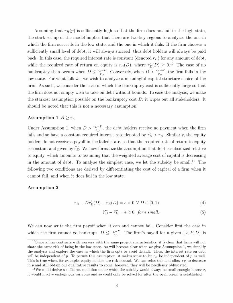
project characterized by p is given by

p [u(V + F )] + (1− p) [u(F − φ)] . (3)

The first term represents the high state of the investment, which occurs with probability

p. In the high state, the worker receives both variable and fixed wages. The second term

represents the low state of the investment, where the worker receives only the fixed wage

and suffers the job termination cost φ.

2.2 Firm Problem

For our empirical analysis in Section 6, we wish to study firms and their associated

workers. We choose to model firm-worker relationships in as simple a way as possible. One

could imagine a matching process in which workers of different skills match with firms of

different risks. This could create potentially interesting dynamics but would only complicate

our analysis. What is important, however, is that firms require workers to implement the

projects in both time periods, i.e., the workers are essential in the production process. We

assume for simplicity that firms are differentiated by the types of workers that are hired. In

other words, firms are differentiated by the riskiness of the projects. To this end, we assume

that a firm hires a measure 1 of workers, each with identical p,9 and raises the required

size 1 of funds. It chooses to raise the funds with debt in the amount of D, where the

remainder, 1 − D, is equity, E. The firm chooses F and V so as to induce the worker to

invest in the project. We assume that firms are risk neutral but are subject to a bankruptcy

cost B, which can sensitize the firm to default risk. In addition, we make the important

assumption that debt is subsidized relative to equity, which will be formalized below. This

is a standard assumption in the corporate finance literature driven largely by a perceived

tax advantage of debt over equity (see, for example, Graham (2000) and references therein).

Since the empirical tests in Section 6 will be performed with data on financial institutions,

it is important to point out that this is also a standard assumption in the banking literature

(see Gorton and Winton (2003) for a discussion).

9The implication of p being identical among workers within a given firm is that firm performance isperfectly correlated with worker performance. Alternatively, we could have firms hire from the entire con-tinuum of workers so that each firm has workers with projects of all levels of risk. The key in that caseis to differentiate and rank firms based on the average risk of the projects that they possess. All that isneeded is positive correlation between worker and firm performance. This relationship is justified based onresults starting with Griliches (1957), in which productivity differences across firms could be explained bydifferences in input quality. In addition, Fox and Smeets (2011) find that differences in labor quality is animportant factor in explaining dispersion in firm performance.

7

Assuming that rH(p) is sufficiently high so that the firm does not fail in the high state,

the stark set-up of the model implies that there are two key regions to analyze: the one in

which the firm succeeds in the low state, and the one in which it fails. If the firm chooses a

sufficiently small level of debt, it will always succeed; thus debt holders will always be paid

back. In this case, the required interest rate is constant (denoted rD) for any amount of debt,

while the required rate of return on equity is rE(D), where r′E(D) ≥ 0.10 The case of no

bankruptcy then occurs when D ≤ rL−FrD

. Conversely, when D > rL−FrD

, the firm fails in the

low state. For what follows, we wish to analyze a meaningful capital structure choice of the

firm. As such, we consider the case in which the bankruptcy cost is sufficiently large so that

the firm does not simply wish to take on debt without bounds. To ease the analysis, we make

the starkest assumption possible on the bankruptcy cost B: it wipes out all stakeholders. It

should be noted that this is not a necessary assumption.

Assumption 1 B ≥ rL

Under Assumption 1, when D > rL−FrD

, the debt holders receive no payment when the firm

fails and so have a constant required interest rate denoted by rD > rD. Similarly, the equity

holders do not receive a payoff in the failed state, so that the required rate of return to equity

is constant and given by rE. We now formalize the assumption that debt is subsidized relative

to equity, which amounts to assuming that the weighted average cost of capital is decreasing

in the amount of debt. To analyze the simplest case, we let the subsidy be small.11 The

following two conditions are derived by differentiating the cost of capital of a firm when it

cannot fail, and when it does fail in the low state.

Assumption 2

rD −Dr′E(D)− rE(D) = ε < 0,∀ D ∈ [0, 1) (4)

rD − rE = ε < 0, for ε small. (5)

We can now write the firm payoff when it can and cannot fail. Consider first the case in

which the firm cannot go bankrupt, D ≤ rL−FrD

. The firm’s payoff for a given {V, F,D} is

10Since a firm contracts with workers with the same project characteristics, it is clear that firms will notshare the same risk of being in the low state. As will become clear when we give Assumption 1, we simplifythe analysis and explore the case in which the firm opts to avoid default. Thus, the interest rate on debtwill be independent of p. To permit this assumption, it makes sense to let rE be independent of p as well.This is true when, for example, equity holders are risk neutral. We can relax this and allow rE to decreasein p and still obtain our qualitative results to come; however, they will be needlessly obfuscated.

11We could derive a sufficient condition under which the subsidy would always be small enough; however,it would involve endogenous variables and so could only be solved for after the equilibrium is established.

8

given by

p [(rH(p)− V − F − rDD]︸ ︷︷ ︸high state return

+(1− p) [rL − F − rDD]︸ ︷︷ ︸low state return

− rE(1−D)︸ ︷︷ ︸opportunity cost of equity capital.

(6)

The first term represents the high state of the investment. rH(p) is earned by the firm from

the investment, V + F is paid to the workers, rDD is paid to the debt holders. The second

term represents the return when the investment is in the low state. Note that only F is paid

to the workers in this case. The final term represents the opportunity cost of equity capital.

Now consider the case in which the firm goes bankrupt in the low state. The firm’s payoff

for a given {V, F,D} is given by

p [rH(p)− V − rD] , (7)

where again rD > rD represents the cost of debt with default risk. The key differences

between (6) and (7) is that, when the investment return is low, there is no payoff for the firm

when it defaults on its debt. In addition, Assumption 1 implies that, upon defaulting, there

is nothing left for the workers nor the debt holders. Therefore, the firm cannot offer a fixed

wage and so is restricted to only using variable wages. Note that limited liability implies

that the payoff in the low state is zero, even if B > rL. We now consider the constrained

optimization problem of the firm both when it can and cannot fail. Consider first the case

in which it cannot fail, D ≤ rL−FrD

.

maxV,F,D

Π = p [rH(p)− V − F −DrD] + (1− p) [rL − F −DrD(D)]− (1−D)rE(D) (8)

subject to p u(V + F ) + (1− p)u(F − φ) ≥ u,

Π ≥ 0.

The first constraint represents the restriction that workers must earn at least their reservation

utility. Given that a firm’s payoff is strictly decreasing in V and F , the Kuhn-Tucker

conditions imply that the worker constraint must hold with equality. Now consider the

problem when the firm fails in the low state, D > rL−FrD

.

maxV,F,D

Π = p [rH(p)− V −DrD] + (1− p) [0]− (1−D)rE (9)

subject to p u(V ) + (1− p)u(−φ) ≥ u,

Π ≥ 0.

9

We solve this problem in two steps. First we determine D∗ and then use that to solve the

appropriate constrained optimization problem. As a consequence of Assumptions 1 and 2, the

firm has only two choices. First, it can choose the highest level of debt that will still maintain

its solvency in all states. Alternatively, it can finance the investment exclusively with debt

and face the bankruptcy cost in the low state. Note again that we are implicitly considering

only the case in which rH(p) is sufficiently large such that the firm is still solvent in the high

state, even when D∗ = 1. The condition under which this is true is rH(p) − V − rD > 0.

Clearly, if this condition does not hold, the result is trivial since the equilibrium, if it exists,

can never involve bankruptcy. This is because either the worker (requiring V ∗) or debt holder

(requiring rD) can never be paid in full. Note also that we will confirm after the equilibrium

analysis that there exists a range of rH(p) such that the firm cannot fail in the high state.

We now show formally that Assumptions 1 and 2 imply that the firm will choose the highest

amount of debt while still avoiding default.

Lemma 1 The firm sets D∗ = rL−FrD

and remains solvent in both states.

Proof. See Appendix.

The intuition behind this result is straightforward. Conditional on no bankruptcy, the

firm payoff is increasing in the amount of debt by Assumption 2. Thus, the firm chooses the

amount of debt, D∗, which just ensures it remains solvent. Conditional on bankruptcy, the

firm chooses to raise the funds completely with debt. Since Assumption 1 sets bankruptcy

costs high, the firm chooses to remain solvent to avoid the cost and so D∗ prevails as the

optimal leverage policy. It is important to point out that, although in our equilibrium the firm

does not go bankrupt, we could enrich the model to allow the firm to endogenously choose

to go bankrupt with some probability. In Section 7, we consider the project/investment with

three potential states instead of two and analyze the case in which the firm chooses to fail

in one of the states. We show there that the results to come still hold.

Given that the solution D∗ implies that equity holders do not receive a payment in the

low state, we define the required rate of return simply by rE since it is constant. We can

now rewrite the firm optimization problem given the solution for D∗ from Lemma 1.

maxV,F

Π = p [rH(p)− V − F − rDD∗]− rE(1−D∗) (10)

subject to p u(V + F ) + (1− p)u(F − φ) ≥ u

Π ≥ 0.

10

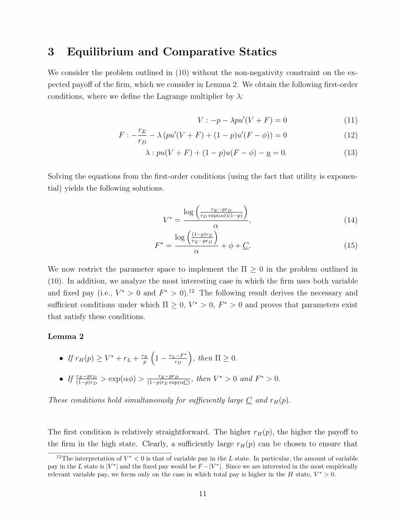
3 Equilibrium and Comparative Statics

We consider the problem outlined in (10) without the non-negativity constraint on the ex-

pected payoff of the firm, which we consider in Lemma 2. We obtain the following first-order

conditions, where we define the Lagrange multiplier by λ:

V : −p− λpu′(V + F ) = 0 (11)

F : −rErD− λ (pu′(V + F ) + (1− p)u′(F − φ)) = 0 (12)

λ : pu(V + F ) + (1− p)u(F − φ)− u = 0. (13)

Solving the equations from the first-order conditions (using the fact that utility is exponen-

tial) yields the following solutions.

V ∗ =log(

rE−prDrD exp(αφ)(1−p)

)α

, (14)

F ∗ =log(

(1−p)rErE−prD

)α

+ φ+ C. (15)

We now restrict the parameter space to implement the Π ≥ 0 in the problem outlined in

(10). In addition, we analyze the most interesting case in which the firm uses both variable

and fixed pay (i.e., V ∗ > 0 and F ∗ > 0).12 The following result derives the necessary and

sufficient conditions under which Π ≥ 0, V ∗ > 0, F ∗ > 0 and proves that parameters exist

that satisfy these conditions.

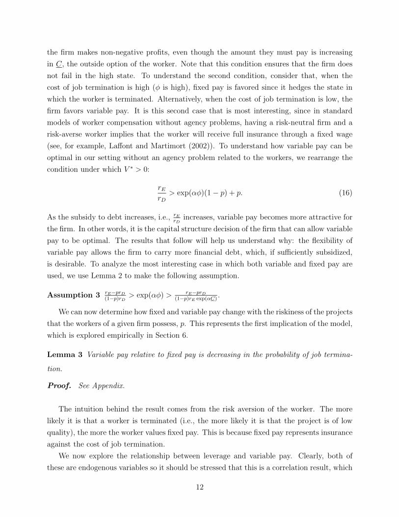
Lemma 2

• If rH(p) ≥ V ∗ + rL + rEp

(1− rL−F ∗

rD

), then Π ≥ 0.

• If rE−prD(1−p)rD

> exp(αφ) > rE−prD(1−p)rE exp(αC)

, then V ∗ > 0 and F ∗ > 0.

These conditions hold simultaneously for sufficiently large C and rH(p).

The first condition is relatively straightforward. The higher rH(p), the higher the payoff to

the firm in the high state. Clearly, a sufficiently large rH(p) can be chosen to ensure that

12The interpretation of V ∗ < 0 is that of variable pay in the L state. In particular, the amount of variablepay in the L state is |V ∗| and the fixed pay would be F−|V ∗|. Since we are interested in the most empiricallyrelevant variable pay, we focus only on the case in which total pay is higher in the H state, V ∗ > 0.

11

the firm makes non-negative profits, even though the amount they must pay is increasing

in C, the outside option of the worker. Note that this condition ensures that the firm does

not fail in the high state. To understand the second condition, consider that, when the

cost of job termination is high (φ is high), fixed pay is favored since it hedges the state in

which the worker is terminated. Alternatively, when the cost of job termination is low, the

firm favors variable pay. It is this second case that is most interesting, since in standard

models of worker compensation without agency problems, having a risk-neutral firm and a

risk-averse worker implies that the worker will receive full insurance through a fixed wage

(see, for example, Laffont and Martimort (2002)). To understand how variable pay can be

optimal in our setting without an agency problem related to the workers, we rearrange the

condition under which V ∗ > 0:

rErD

> exp(αφ)(1− p) + p. (16)

As the subsidy to debt increases, i.e., rErD

increases, variable pay becomes more attractive for

the firm. In other words, it is the capital structure decision of the firm that can allow variable

pay to be optimal. The results that follow will help us understand why: the flexibility of

variable pay allows the firm to carry more financial debt, which, if sufficiently subsidized,

is desirable. To analyze the most interesting case in which both variable and fixed pay are

used, we use Lemma 2 to make the following assumption.

Assumption 3 rE−prD(1−p)rD

> exp(αφ) > rE−prD(1−p)rE exp(αC)

.

We can now determine how fixed and variable pay change with the riskiness of the projects

that the workers of a given firm possess, p. This represents the first implication of the model,

which is explored empirically in Section 6.

Lemma 3 Variable pay relative to fixed pay is decreasing in the probability of job termina-

tion.

Proof. See Appendix.

The intuition behind the result comes from the risk aversion of the worker. The more

likely it is that a worker is terminated (i.e., the more likely it is that the project is of low

quality), the more the worker values fixed pay. This is because fixed pay represents insurance

against the cost of job termination.

We now explore the relationship between leverage and variable pay. Clearly, both of

these are endogenous variables so it should be stressed that this is a correlation result, which

12

is explored empirically in Section 6.

Lemma 4 Debt is negatively correlated with the amount of fixed pay, and positively corre-

lated with the amount of variable pay relative to fixed pay.

Proof. See Appendix.

We show this result by analyzing the relationship between every exogenous variable that

affects both the amount of debt and the worker compensation. In each case, the sign of the

derivative is the opposite for debt versus that of fixed pay, and the same for debt versus

that of variable pay relative to fixed pay. Note that there is one exogenous variable, rL, that

affects only the amount of debt. To understand this result, it is illuminating to consider the

bankruptcy costs of debt, and the fact that debt is subsidized relative to equity. Given these

two features, the firm wishes to take on the most debt that it can, while avoiding bankruptcy.

Fixed pay is essentially debt on the operating side of the firm. The more fixed pay that the

firm uses, the less financial debt that the firm can sustain. Thus, if the relative amount

of fixed pay decreases (due to a change in an exogenous parameter of our model), the firm

can take on more financial debt. It is now straightforward to give the main implication of

our model, which will be explored empirically in Section 6. The following result gives the

relationship between the probability of job termination and the capital structure of the firm.

Proposition 1 The higher the probability of job termination, the less debt a firm will em-

ploy.

Proof. See Appendix.

The intuition behind this result is found easily by considering Lemmas 3 and 4. The

higher the probability of job termination, the more fixed pay relative to variable pay (and

the more fixed pay in absolute terms) that workers will be paid. The more fixed pay, the

less debt a firm can employ.

3.1 The Optimal Decision at t = 1

The decision made by the firm between t = 1 and t = 2 differs based on whether the

worker’s investment is in the high or low state. Recall that we assumed that a worker is

essential at both time periods, so that the firm must continue to employ workers to realize

any payoff at t = 2. Define V 2H (F 2

H) as variable (fixed) wage at time t = 2 if the state is H,

13

r2D as the required rate of return to debt, and r2E as the required rate of return to equity. If

the investment is in the high state, then it returns rH(p) with certainty. Since debt is again

assumed to be subsidized, the firm optimally sets D∗ = 1 since it cannot go bankrupt.13 The

firm problem becomes

maxV 2H ,F

2H

rH(p)− V 2H − F 2

H − r2D subject to: u(V 2H + F 2

H) ≥ u. (17)

It is straightforward to show that the choice between fixed and variable pay is irrelevant

since variable pay is not actually variable. Thus, the solution is simply given by the firm

paying the worker C2 = C with certainty, namely the outside option. If the investment is in

the low state, there is no further payoff for the firm, and thus the budget constraint cannot

hold since the firm would lose money by paying C. Thus, it is optimal to terminate the

worker.14

It is important to recognize that this decision is made at t = 1 and therefore has no

bearing on the decision at t = 0. If we relaxed the assumption that the worker does not

discount utility over the three periods, it will have no effect on the solution at t = 0.

4 Applications to Financial Institutions

Our empirical application in Section 6 tests the results outlined in Section 3 using data

from financial institutions. It is therefore worth exploring additional theoretical implications

of our model as they apply to these types of firms. Our model is able to rationalize two

key features of financial institutions. First, a typical debt-to-assets ratio for non-financial

corporations is around 20% to 30%, whereas for financial institutions it is closer to 87%

to 95% (Gornall and Strebulaev (2014)). Second, Lemieux et al. (2009) for the U.S. and

Celerier and Vallee (2015) for France show that, on average, financial institutions pay 65%

of a worker’s salary as variable compensation. This compares with 33% to 41% in non-

financial firms (Lemieux et al. (2009) and Celerier and Vallee (2015), respectively). We

show that these two features can arise endogenously through each of two parameters: the

13In reality, the firm may choose to use profits from the previous period for the investment. Since thecapital structure choice at t = 1 is not particularly important relative to that at t = 0, we will not pursuethis further in detail. One can assume that the firm invests in the debt to account for what is done withthe profits from the investment between t = 0 and t = 1. Note again that we are implicitly assuming thatrH(p) is sufficiently large that the firm is still solvent when D∗ = 1. The condition under which this is trueis rH(p)− V 2

H − F 2H − r2D > 0.

14Note that a worker still receives the outside option C when terminated; however, it is not received fromthe firm in question.

14

cost of job termination and the cost of debt. We consider below that both the cost of

job termination and the cost of debt is, on average, lower in financial institutions versus

non-financial institutions.

4.1 The Cost of Job Termination

Consider the cost of job termination within financial institutions; Jacobson et al. (1994)

report that, in the U.S., the financial sector is among the lowest in terms of future losses to

the worker upon job displacement. Morissette et al. (2007) find similar evidence for Canada.

Explanations of why the financial industry has a lower cost to a worker of being displaced

typically revolve around the lack of unionization (for example, according to Statistics Canada,

the rate of unionization in finance in Canada is around 7.5%) and the relatively portable skills

that finance employees have when moving within industry.15 The following result formalizes

the relationship in the model.

Corollary 1 The lower the cost of job termination

i. The more variable pay relative to fixed pay a firm will use.

ii. The more debt that a firm will employ.

Proof. See Appendix.

The result is due to the low cost of job termination resulting in a higher level of vari-

able wages, which consequently lead to higher levels of leverage. Therefore, since financial

institutions have on average a lower cost of job termination, we should expect to see more

variable wages relative to fixed wages and a higher leverage in financial institutions relative

to non-financial institutions.

4.2 The Cost of Debt

There are a number of reasons why financial firms can enjoy better borrowing rates than

those for non-financial firms. Banks that hold deposits receive a subsidy through deposit

15For example, Morris and Wilhelm (2007) argue that investment bankers posses largely industry-specifichuman capital and, if there is any firm-specific human capital that exists, it is largely a cultural differencebetween firms. Even then, investment bankers have reduced the cost by sometimes migrating as teams. Manyfinancial institutions will also penalize bankers who leave voluntarily (but not when they are terminated)by confiscating vested options (thereby increasing switching costs). This practice suggests that the cost ofleaving the firm may be low since firms attempt to raise the cost for workers who leave on their own.

15

insurance (see, for example, Allen et al. (2014)). Broker-dealers, which will the focus of

the empirical investigation in Section 6, receive this subsidy indirectly when they are owned

by a deposit-taking institution. Financial institutions also tend to have highly liquid debt

(Diamond and Dybvig (1983)). The broker-dealers in the data to be introduced in Section

5 have on average approximately 90% of their liabilities classified as liquid.16 In our model,

the cost of debt is affected by the bankruptcy cost since that cost directly affects recovery

rates.17 In addition, financial institutions such as broker-dealers have highly liquid assets in

case of fire sales.18 Finally, financial institutions tend to have better contract re-enforcement

than non-financial institutions (Holmstrom and Tirole (1997)). The following result relates

the cost of debt to the amount of variable pay that a firm will use.

Corollary 2 The lower the cost of debt

i. The more variable pay relative to fixed pay the firm will use.

ii. The more debt a firm will employ.

Proof. See Appendix.

The second part of the result is straightforward: the lower the cost of debt, the more

debt a firm wishes to take on. To take advantage of the lower cost of debt, however, the

firm lowers the amount of fixed pay it uses to compensate workers to avoid the potential

bankruptcy costs. Of course, if fixed pay is lower, the firm must increase variable pay so as

to keep the worker at least as well off. Thus, a lower cost of debt of financial institutions

works in the same way as a lower cost of job termination: we should expect to see financial

institutions employ more debt and more variable pay relative to non-financial institutions.

5 Data

The data set we rely on to test the model predictions is a complete proprietary panel

of investment brokers and dealers in Canada from January 1992 to December 2010. This

16Major categories of liabilities include current liabilities (overdrafts, loans payable, securities loans, andrepurchase agreements, securities sold short, and client accounts), long-term liabilities (deferred income taxesand capitalized leases), and financial capital.

17It is important to note that, although Assumption 1 implies that recovery rates are always zero, it isnot a necessary assumption. We can obtain all the results in the paper when recovery rates are positive sothat an increase in bankruptcy costs causes the cost of debt to increase.

18Liquid assets include cash, loans receivables, securities borrowed and resold, securities owned by thefirm and their clients, and clients accounts. Other allowable assets include receivables and recoverableand overpaid taxes. Non-allowable (illiquid) assets include receivables, fixed assets, capitalized leases, andinvestments in subsidiaries, among other items. Non-allowable assets make up, on average 10% of assets.

16

includes banks as well as large and small institutional and retail investors. These data

are collected by the Investment Industry Regulatory Organization of Canada (IIROC) and

include monthly regulatory financial reports (Form 1 of the IIROC Rule Book).19 Income

and balance sheet data are reported monthly although we aggregate annually; bonuses are

accrued monthly but paid annually, and what is accrued might not actually be awarded.

Therefore using monthly data would not be appropriate for analyzing questions related

to compensation. IIROC’s membership grew from 119 in 1992 to 201 by 2010 but also

experienced exits and several mergers. We drop firms that appear for fewer than 5 years and

keep track of all mergers.20

IIROC is a self-regulatory organization that oversees investment dealer activity in debt

and equity markets in Canada as well as personal and wholesale investing. In terms of pru-

dential requirements, IIROC enforces a minimum capital requirement (risk-adjusted capital)

and also requires that members hold more margin for assets that are riskier and less liq-

uid. They are also the market-conduct regulators, monitoring dealer behavior, and ensuring

members follow a set of Market Integrity Practices that govern issues like front-running and

client priority.

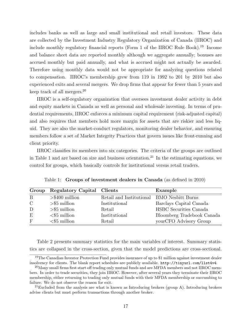
IIROC classifies its members into six categories. The criteria of the groups are outlined

in Table 1 and are based on size and business orientation.21 In the estimating equations, we

control for groups, which basically controls for institutional versus retail traders.

Table 1: Groups of investment dealers in Canada (as defined in 2010)

Group Regulatory Capital Clients Example

B >$400 million Retail and Institutional BMO Nesbitt BurnsC >$5 million Institutional Barclays Capital CanadaD >$5 million Retail HSBC Securities CanadaE <$5 million Institutional Bloomberg Tradebook CanadaF <$5 million Retail yourCFO Advisory Group

Table 2 presents summary statistics for the main variables of interest. Summary statis-

tics are collapsed in the cross-section, given that the model predictions are cross-sectional.

19The Canadian Investor Protection Fund provides insurance of up to $1 million against investment dealerinsolvency for clients. The blank report schedules are publicly available. http://tinyurl.com/llst4v4.

20Many small firms first start off trading only mutual funds and are MFDA members and not IIROC mem-bers. In order to trade securities, they join IIROC. However, after several years they terminate their IIROCmembership, either returning to trading only mutual funds with their MFDA membership or succumbing tofailure. We do not observe the reason for exit.

21Excluded from the analysis are what is known as Introducing brokers (group A). Introducing brokersadvise clients but must perform transactions through another broker.

17

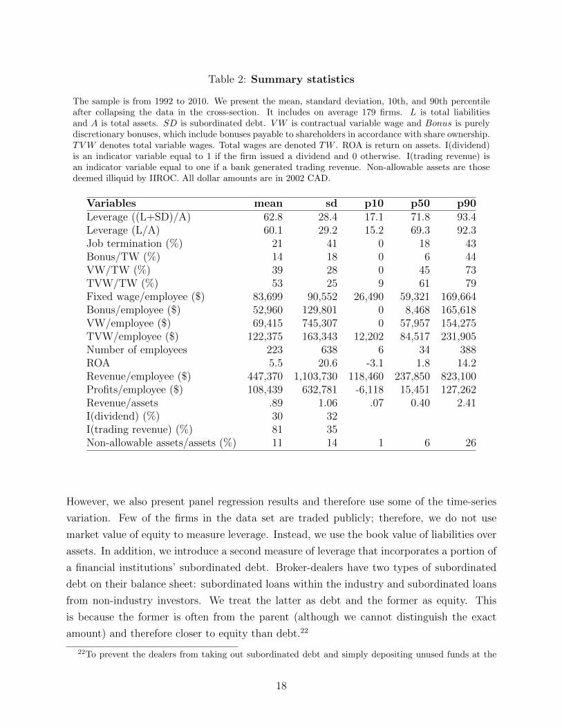
Table 2: Summary statistics

The sample is from 1992 to 2010. We present the mean, standard deviation, 10th, and 90th percentileafter collapsing the data in the cross-section. It includes on average 179 firms. L is total liabilitiesand A is total assets. SD is subordinated debt. VW is contractual variable wage and Bonus is purelydiscretionary bonuses, which include bonuses payable to shareholders in accordance with share ownership.TVW denotes total variable wages. Total wages are denoted TW . ROA is return on assets. I(dividend)is an indicator variable equal to 1 if the firm issued a dividend and 0 otherwise. I(trading revenue) isan indicator variable equal to one if a bank generated trading revenue. Non-allowable assets are thosedeemed illiquid by IIROC. All dollar amounts are in 2002 CAD.

Variables mean sd p10 p50 p90Leverage ((L+SD)/A) 62.8 28.4 17.1 71.8 93.4Leverage (L/A) 60.1 29.2 15.2 69.3 92.3Job termination (%) 21 41 0 18 43Bonus/TW (%) 14 18 0 6 44VW/TW (%) 39 28 0 45 73TVW/TW (%) 53 25 9 61 79Fixed wage/employee ($) 83,699 90,552 26,490 59,321 169,664Bonus/employee ($) 52,960 129,801 0 8,468 165,618VW/employee ($) 69,415 745,307 0 57,957 154,275TVW/employee ($) 122,375 163,343 12,202 84,517 231,905Number of employees 223 638 6 34 388ROA 5.5 20.6 -3.1 1.8 14.2Revenue/employee ($) 447,370 1,103,730 118,460 237,850 823,100Profits/employee ($) 108,439 632,781 -6,118 15,451 127,262Revenue/assets .89 1.06 .07 0.40 2.41I(dividend) (%) 30 32I(trading revenue) (%) 81 35Non-allowable assets/assets (%) 11 14 1 6 26

However, we also present panel regression results and therefore use some of the time-series

variation. Few of the firms in the data set are traded publicly; therefore, we do not use

market value of equity to measure leverage. Instead, we use the book value of liabilities over

assets. In addition, we introduce a second measure of leverage that incorporates a portion of

a financial institutions’ subordinated debt. Broker-dealers have two types of subordinated

debt on their balance sheet: subordinated loans within the industry and subordinated loans

from non-industry investors. We treat the latter as debt and the former as equity. This

is because the former is often from the parent (although we cannot distinguish the exact

amount) and therefore closer to equity than debt.22

22To prevent the dealers from taking out subordinated debt and simply depositing unused funds at the

18

Our results are qualitatively similar when industry-subordinated debt is included; how-

ever, leverage is substantially higher in some cases. Nevertheless, the average broker-dealer

leverage is around 62% while median leverage is 70%. The 90th-percentile firm leverage is

93%. Note that Crawford et al. (2009) highlight the role of regulatory limits on assets-

to-capital ratios in Canada and therefore lower leverage, on average, for Canadian banks

relative to those in the U.K., U.S., and continental Europe. Therefore, leverage as we define

it is slightly lower, on average, in our sample relative to what is reported for the United

States in Gornall and Strebulaev (2014).

Our measure of job termination is firm-specific. A firm is given a 1 if, at between

t − 1 and t, it laid off at least 5% of its workforce and 0 otherwise.23 Our interpretation

is that workers in firms with high turnover are more likely to experience job termination.

In our econometric specifications, we look at within-firm and between-firm variation in job

termination and its correlation with pay and leverage. On average, 21% of firms experience

job termination of at least 5%. Note that, in the data, we cannot separately identify firing

from voluntary departures. There are a number of reasons why job termination in this

industry, however, might not be considered voluntary. First, almost all firms have a no-

competitor clause, typically 6 months to 1 year if an employee leaves a firm voluntarily. This

introduces an important switching cost. In addition, bonuses are often deferred, especially

any stock options, which can lead to large switching costs for voluntary departure (Morris and

Wilhelm (2007)).24 Third, investment bankers do rotate across institutions, but this occurs

only when there is strong signalling about their job prospects at their current placement.

For wages, they are decomposed into three segments.25 First is fixed wages. Fixed

wages are included in total operating expenses. For about a dozen financial institutions,

we have the breakdown of operating expenses into wages and other expenses through access

to the confidential Canadian tri-agency database managed by the Bank of Canada, the

provider of the debt (likely their parent), IIROC introduced a provider of capital concentration chargein January 2000. Standby subordinated loans for the most part found their way into subordinated loansfrom industry investors where “Industry Investors” refer to individuals who own a beneficial interest in aninvestment in the Dealer Member or holding company (of the Dealer Member) (IIROC, accessed 2011). Byanalyzing the capital charges, we are able to determine that within-industry subordinated loans are largelyfrom the parent.

23For robustness, we also look at 7.5% and 10% and have qualitatively similar results. The idea is tocapture firms that lay off a significant fraction of their workforce.

24Aldatmaz et al. (2014) find that turnover falls following broad-based employee stock options, althoughthe effect is temporary.

25Wages are based on average wages for all non-executive broker-dealers in the firm, irrespective of hierar-chy. Efing et al. (2014) do not find that the correlation between variable pay and trading volume/volatilty issensitive to whether or not wages are equally weighted or weighted by hierarchy within their set of Europeanbanks. This provides some assurance that our approach, which is used because of the lack of information onjob titles, is sufficient to capture the cross-section heterogeneity in firms’ wages.

19

Office of the Superintendent of Financial Institutions, and the Canada Deposit Insurance

Corporation. Wages are consistently 50% of operating expenses; therefore, we apply this rule

for all financial institutions. This is admittedly ad hoc, but in effect only scales our measure of

total wages, given that there is almost no variation in the composition of operating expenses.

In addition, there are two types of bonuses. Variable compensation (VW ) includes all other

bonuses, such as commissions and other bonuses of a contractual nature. Importantly, these

are payouts only to registered representatives and institutional and professional trading

personnel. Bonuses to management are not included, both discretionary and contractual.

Second, there are discretionary bonuses (bonus), which include all discretionary bonuses,

including dividends to shareholders (those who are employees).

Total wages is the sum of its three components. In Canadian dollars (deflated using

the 1992 consumer price index deflator), the average base (or fixed) wage per employee

is approximately $83,699 (or approximately $104,127 in 2014). Discretionary bonuses are

on average $52,960 per employee. However, about 10% of firms never pay a discretionary

bonus. Variable wages are on average $69,415 per employee and, similar to discretionary

bonuses, about 10% of firms do not pay variable wages. Interestingly, these are not necessarily

the same 10% as those that do not pay discretionary bonuses. Firms that do not pay

discretionary bonuses tend to be in group F, i.e., small retail firms. Firms that tend not to

pay contractual bonuses tend to be an equal mix of firms in group F and firms in group C,

i.e., large institutional firms. On average, total wages are similar to those reported in the

introduction for analysts and specialists.

The average return on assets is 4.74 and there is substantial variation. The ROA for

the broker-dealers in this sample is substantially higher than that reported for the banking

sector, which is closer to 1. We report a median ROA of 1.8, however, which is closer to what

one would expect in the banking sector. Given the extreme outliers that generate the large

differences in the mean and median, we winsorize the data at the 1% level before estimating

our econometric specifications. We also report revenue per employee and revenue per asset.

Each employee, on average, generates $447,370 per year (approximately $556,560 in 2014

dollars) with substantial variation across firms and time. Profits are approximately $108,000

per year per employee. An average firm has 223 employees, where employee includes only

registered representatives of the firm. A dollar of assets generates about 89 cents of revenue.

Finally, about 81% of firms are involved in trading. A small fraction of firms specialize in

only mergers and acquisitions.

20

6 Empirical Results

Our model of capital structure and pay structure has three testable implications. First

is Lemma 3: variable pay as a fraction of total compensation is decreasing in the probability

of job termination. Second is Lemma 4: debt is negatively correlated with the amount

of fixed pay and positively correlated with the amount of variable pay relative to fixed pay.

Finally, Proposition 1 – the main result of the paper – is that the higher the probability of job

termination, the less debt a firm will employ. In this section, we present empirical tests for the

model’s predictions. All three empirical predictions are cross-sectional. Given that our data

are annual over a long time period, we present results both from pooled OLS regressions and

the between estimator. The pooled OLS estimator takes into account both the cross-section

and time-series variation. The between estimator uses only the cross-sectional information

by averaging the within-firm information.

Our first regression has total variable wages (variable wage plus discretionary bonuses)

as a fraction of total wages as the dependent variable and the main independent variable is

the probability of job termination. The prediction from Lemma 3 is that β < 0.

TVW/TWit = α + βpr(job termination)it + γXit + δj + εit. (18)

Included in the Xs are ROA, log of total assets (size), revenue/assets, an indicator variable

for whether or not the firm paid dividends and an indicator variable for whether or not the

firm generated trading income; δ captures group fixed effects where the groups are B-F as

defined in Section 5. This variable largely captures whether a firm is institutional versus

retail. We include size as a control for several reasons. The main one, however, is that there is

evidence that firms offer increasing wage profiles to loosen the effects of financial constraints

(Michelacci and Quadrini (2008)). In our context, this implies smaller firms would have a

larger fraction of their wage flexible relative to that of the larger firms. The pooled OLS

estimator uses all of the information in i and t, whereas the between estimator averages the

information over t, and β captures the correlation between wages and the probability of job

termination across the i firms.

Results from estimating equation (18) by pooled OLS are presented in column (1) of Table

3. In addition, we present results using a between estimator in column (2) and the marginal

effects from the Logit model in column (3), given that some firms do not pay variable wages.

The model predictions are in the cross-section; therefore, our main focus is in on column (2).

Our variables capture nearly 30% of the cross-sectional variation in wage structure. Firms

that are more likely to have turnover are less likely to use variable wages and therefore more

21

likely to use fixed wages. Therefore, this result provides supporting evidence for Lemma 3.

How much less? A firm with high turnover pays 27.9% less variable pay relative to fixed pay

than a firm with low turnover. If we look at columns (1) and (3), where we combine the

cross-section and time-series data, the impact of job termination on wages is less but still

substantial. We can also see that the impact of zeros is minimal, given that the difference

in the coefficients from (1) to (3) is negligible.

Lastly, in addition to our main variable of interest, we do not find a positive correlation

between size and the wage structure. We do, however, document a positive correlation

between total variable compensation and revenue/assets as well as between total variable

compensation and dividend payouts. We also document a negative correlation with non-

allowable assets (illiquidity) and ROA. The more illiquid a banks’ portfolio or the lower the

ROA, the higher the fraction of pay that is fixed. This is consistent with results in the next

table, Table 4, where we show based on the cross-sectional variation, that job separation

and firm risk, measured by volatility in ROA, as well as volatility in firm revenue per assets

and firm profits per assets, is positive.26 Importantly, the results from Table 4 act as a check

on our theory. The model is constructed such that workers with riskier projects are more

likely to be terminated. When workers have riskier projects, the corresponding firm should

be riskier in the model. Thus, we should expect to see a positive relationship in the data

between firm risk and the probability of job separation, which can be seen in Table 4.

The second estimating equation is given by (19) and has leverage as the dependent

variable and the fraction of total compensation as the main independent variable of interest.

The model prediction is that β > 0. Strictly speaking, Lemma 4 only states that leverage

and variable wages are positively correlated and not that variable wages as a fraction total

wages causes leverage. Note that the Xs and δj are as before. We do, however, include

lagged leverage in the pooled OLS version to capture the idea that leverage is persistent

(Gropp and Heider (2010)).

Lit = α + ρLi,t−1 + β(VW/TW )it + γXit + δj + εit. (19)

We show results from two approaches, pooled OLS in columns (1)–(2) of Table 5 and a

between estimator in columns (3)–(4) of the same table.

The results from Table 5 suggest that leverage is highly persistent. This is consistent

with the literature. Second, and the focus of this paper, is that total variable compensation

26In the model, what is important is that firm risk is the probability of project success, and not liquidationfrom leverage risk. Empirically, there is no exact counterpart. We therefore measure risk in the probabilityof project success using three different balance sheet figures: volatility in revenues, profits, and return onassets.

22

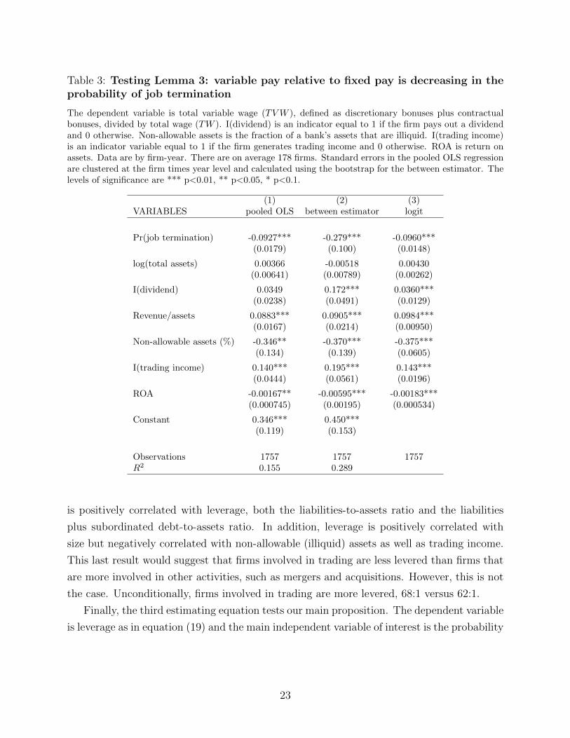
Table 3: Testing Lemma 3: variable pay relative to fixed pay is decreasing in theprobability of job termination

The dependent variable is total variable wage (TVW ), defined as discretionary bonuses plus contractualbonuses, divided by total wage (TW ). I(dividend) is an indicator equal to 1 if the firm pays out a dividendand 0 otherwise. Non-allowable assets is the fraction of a bank’s assets that are illiquid. I(trading income)is an indicator variable equal to 1 if the firm generates trading income and 0 otherwise. ROA is return onassets. Data are by firm-year. There are on average 178 firms. Standard errors in the pooled OLS regressionare clustered at the firm times year level and calculated using the bootstrap for the between estimator. Thelevels of significance are *** p<0.01, ** p<0.05, * p<0.1.

(1) (2) (3)VARIABLES pooled OLS between estimator logit

Pr(job termination) -0.0927*** -0.279*** -0.0960***(0.0179) (0.100) (0.0148)

log(total assets) 0.00366 -0.00518 0.00430(0.00641) (0.00789) (0.00262)

I(dividend) 0.0349 0.172*** 0.0360***(0.0238) (0.0491) (0.0129)

Revenue/assets 0.0883*** 0.0905*** 0.0984***(0.0167) (0.0214) (0.00950)

Non-allowable assets (%) -0.346** -0.370*** -0.375***(0.134) (0.139) (0.0605)

I(trading income) 0.140*** 0.195*** 0.143***(0.0444) (0.0561) (0.0196)

ROA -0.00167** -0.00595*** -0.00183***(0.000745) (0.00195) (0.000534)

Constant 0.346*** 0.450***(0.119) (0.153)

Observations 1757 1757 1757R2 0.155 0.289

is positively correlated with leverage, both the liabilities-to-assets ratio and the liabilities

plus subordinated debt-to-assets ratio. In addition, leverage is positively correlated with

size but negatively correlated with non-allowable (illiquid) assets as well as trading income.

This last result would suggest that firms involved in trading are less levered than firms that

are more involved in other activities, such as mergers and acquisitions. However, this is not

the case. Unconditionally, firms involved in trading are more levered, 68:1 versus 62:1.

Finally, the third estimating equation tests our main proposition. The dependent variable

is leverage as in equation (19) and the main independent variable of interest is the probability

23

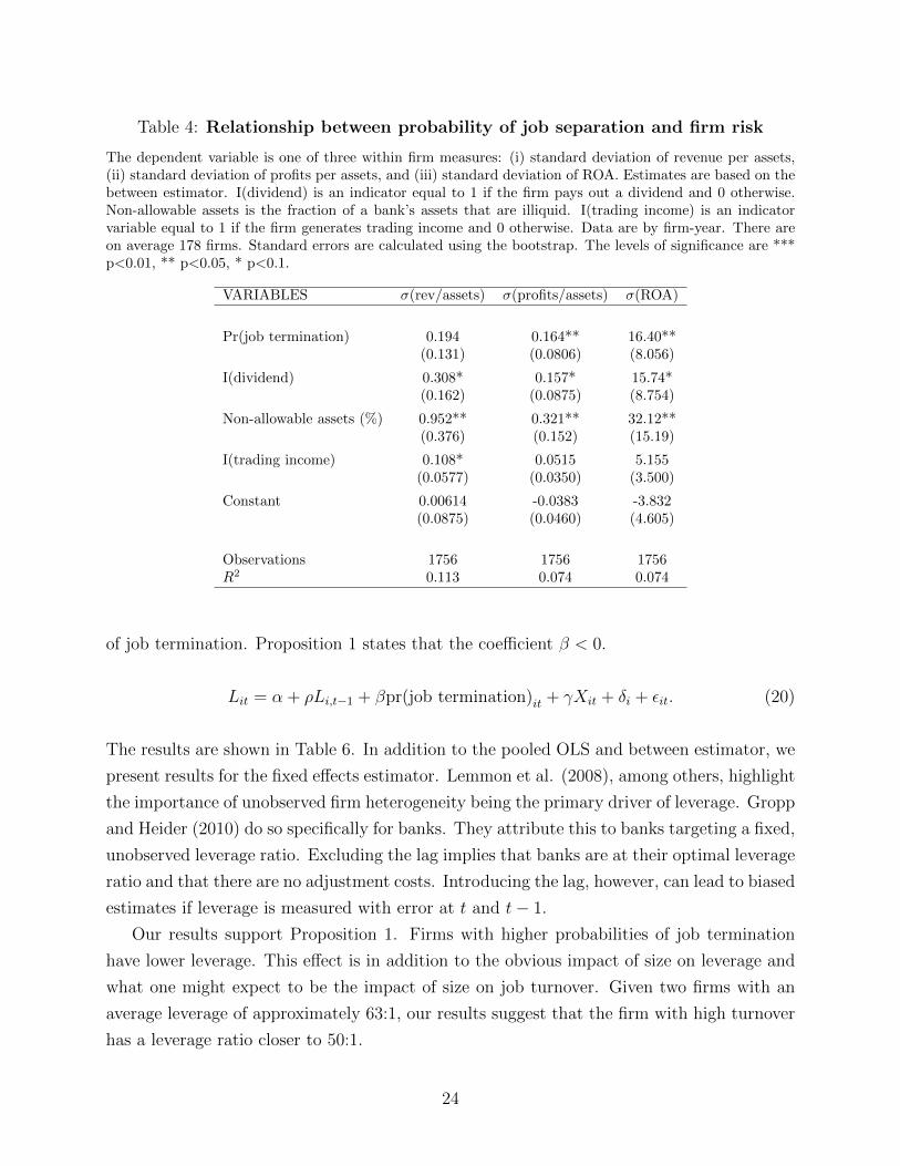
Table 4: Relationship between probability of job separation and firm risk

The dependent variable is one of three within firm measures: (i) standard deviation of revenue per assets,(ii) standard deviation of profits per assets, and (iii) standard deviation of ROA. Estimates are based on thebetween estimator. I(dividend) is an indicator equal to 1 if the firm pays out a dividend and 0 otherwise.Non-allowable assets is the fraction of a bank’s assets that are illiquid. I(trading income) is an indicatorvariable equal to 1 if the firm generates trading income and 0 otherwise. Data are by firm-year. There areon average 178 firms. Standard errors are calculated using the bootstrap. The levels of significance are ***p<0.01, ** p<0.05, * p<0.1.

VARIABLES σ(rev/assets) σ(profits/assets) σ(ROA)

Pr(job termination) 0.194 0.164** 16.40**(0.131) (0.0806) (8.056)

I(dividend) 0.308* 0.157* 15.74*(0.162) (0.0875) (8.754)

Non-allowable assets (%) 0.952** 0.321** 32.12**(0.376) (0.152) (15.19)

I(trading income) 0.108* 0.0515 5.155(0.0577) (0.0350) (3.500)

Constant 0.00614 -0.0383 -3.832(0.0875) (0.0460) (4.605)

Observations 1756 1756 1756R2 0.113 0.074 0.074

of job termination. Proposition 1 states that the coefficient β < 0.

Lit = α + ρLi,t−1 + βpr(job termination)it + γXit + δi + εit. (20)

The results are shown in Table 6. In addition to the pooled OLS and between estimator, we

present results for the fixed effects estimator. Lemmon et al. (2008), among others, highlight

the importance of unobserved firm heterogeneity being the primary driver of leverage. Gropp

and Heider (2010) do so specifically for banks. They attribute this to banks targeting a fixed,

unobserved leverage ratio. Excluding the lag implies that banks are at their optimal leverage

ratio and that there are no adjustment costs. Introducing the lag, however, can lead to biased

estimates if leverage is measured with error at t and t− 1.

Our results support Proposition 1. Firms with higher probabilities of job termination

have lower leverage. This effect is in addition to the obvious impact of size on leverage and

what one might expect to be the impact of size on job turnover. Given two firms with an

average leverage of approximately 63:1, our results suggest that the firm with high turnover

has a leverage ratio closer to 50:1.

24

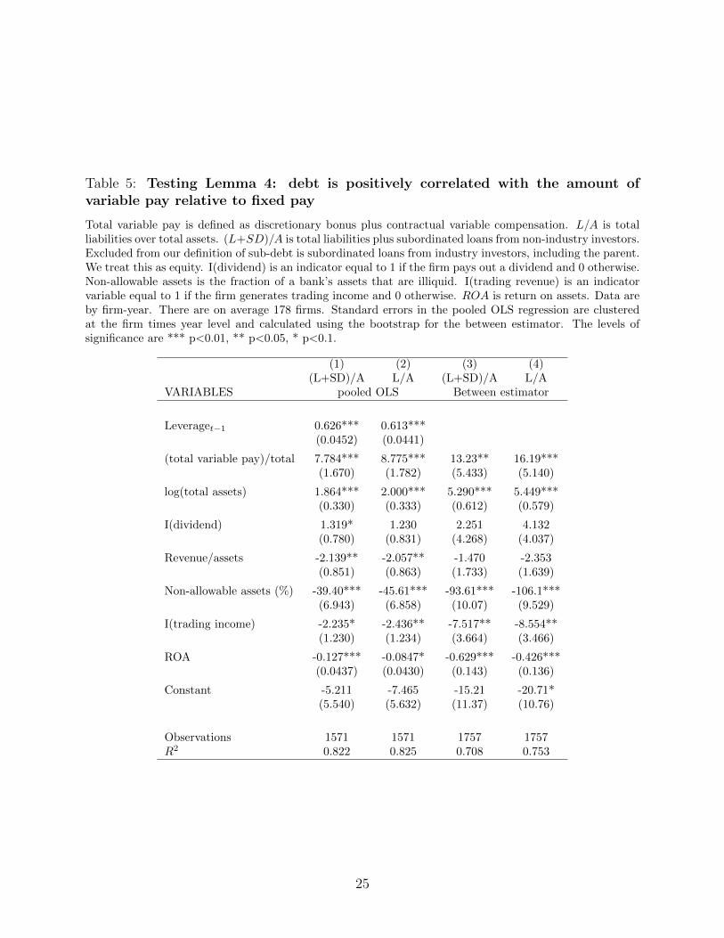
Table 5: Testing Lemma 4: debt is positively correlated with the amount ofvariable pay relative to fixed pay

Total variable pay is defined as discretionary bonus plus contractual variable compensation. L/A is totalliabilities over total assets. (L+SD)/A is total liabilities plus subordinated loans from non-industry investors.Excluded from our definition of sub-debt is subordinated loans from industry investors, including the parent.We treat this as equity. I(dividend) is an indicator equal to 1 if the firm pays out a dividend and 0 otherwise.Non-allowable assets is the fraction of a bank’s assets that are illiquid. I(trading revenue) is an indicatorvariable equal to 1 if the firm generates trading income and 0 otherwise. ROA is return on assets. Data areby firm-year. There are on average 178 firms. Standard errors in the pooled OLS regression are clusteredat the firm times year level and calculated using the bootstrap for the between estimator. The levels ofsignificance are *** p<0.01, ** p<0.05, * p<0.1.

(1) (2) (3) (4)(L+SD)/A L/A (L+SD)/A L/A

VARIABLES pooled OLS Between estimator

Leveraget−1 0.626*** 0.613***(0.0452) (0.0441)

(total variable pay)/total 7.784*** 8.775*** 13.23** 16.19***(1.670) (1.782) (5.433) (5.140)

log(total assets) 1.864*** 2.000*** 5.290*** 5.449***(0.330) (0.333) (0.612) (0.579)

I(dividend) 1.319* 1.230 2.251 4.132(0.780) (0.831) (4.268) (4.037)

Revenue/assets -2.139** -2.057** -1.470 -2.353(0.851) (0.863) (1.733) (1.639)

Non-allowable assets (%) -39.40*** -45.61*** -93.61*** -106.1***(6.943) (6.858) (10.07) (9.529)

I(trading income) -2.235* -2.436** -7.517** -8.554**(1.230) (1.234) (3.664) (3.466)

ROA -0.127*** -0.0847* -0.629*** -0.426***(0.0437) (0.0430) (0.143) (0.136)

Constant -5.211 -7.465 -15.21 -20.71*(5.540) (5.632) (11.37) (10.76)

Observations 1571 1571 1757 1757R2 0.822 0.825 0.708 0.753

25

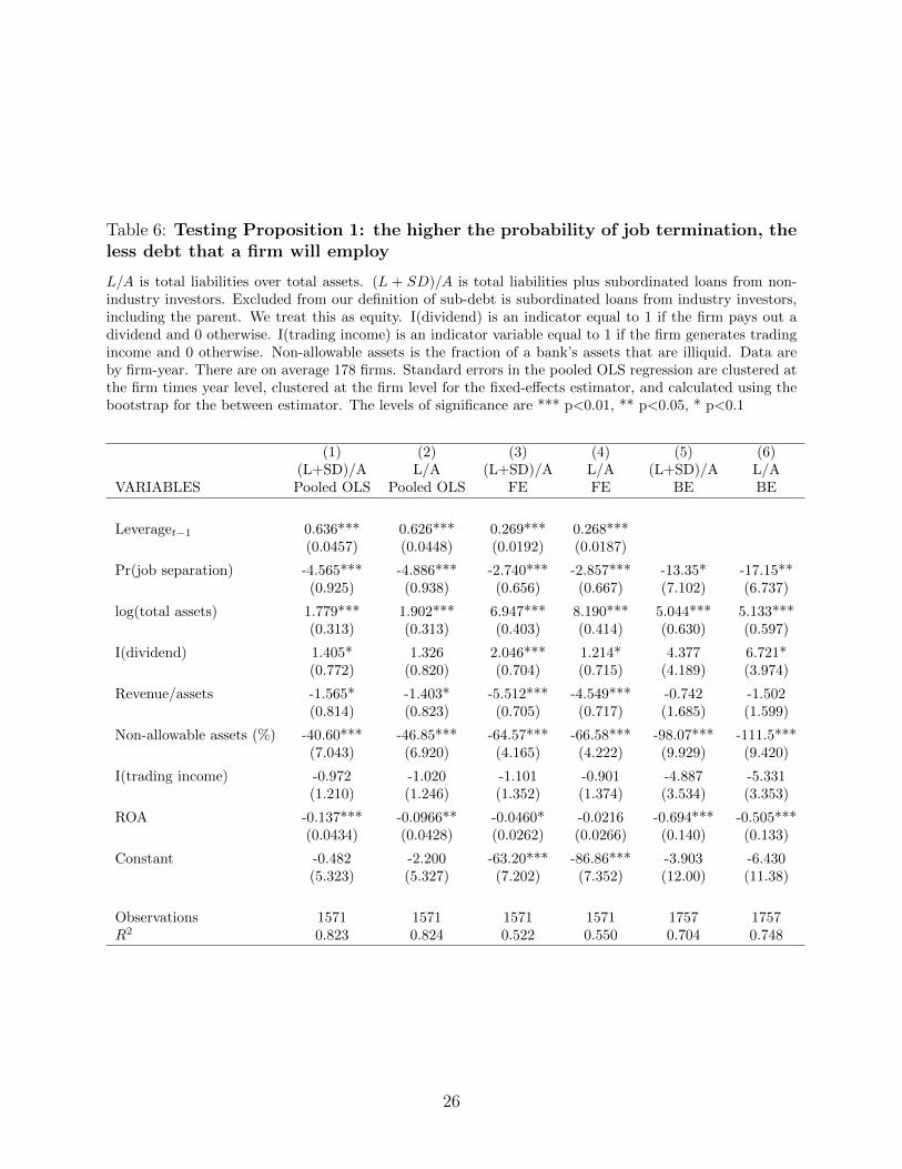
Table 6: Testing Proposition 1: the higher the probability of job termination, theless debt that a firm will employ

L/A is total liabilities over total assets. (L + SD)/A is total liabilities plus subordinated loans from non-industry investors. Excluded from our definition of sub-debt is subordinated loans from industry investors,including the parent. We treat this as equity. I(dividend) is an indicator equal to 1 if the firm pays out adividend and 0 otherwise. I(trading income) is an indicator variable equal to 1 if the firm generates tradingincome and 0 otherwise. Non-allowable assets is the fraction of a bank’s assets that are illiquid. Data areby firm-year. There are on average 178 firms. Standard errors in the pooled OLS regression are clustered atthe firm times year level, clustered at the firm level for the fixed-effects estimator, and calculated using thebootstrap for the between estimator. The levels of significance are *** p<0.01, ** p<0.05, * p<0.1

(1) (2) (3) (4) (5) (6)(L+SD)/A L/A (L+SD)/A L/A (L+SD)/A L/A

VARIABLES Pooled OLS Pooled OLS FE FE BE BE

Leveraget−1 0.636*** 0.626*** 0.269*** 0.268***(0.0457) (0.0448) (0.0192) (0.0187)

Pr(job separation) -4.565*** -4.886*** -2.740*** -2.857*** -13.35* -17.15**(0.925) (0.938) (0.656) (0.667) (7.102) (6.737)

log(total assets) 1.779*** 1.902*** 6.947*** 8.190*** 5.044*** 5.133***(0.313) (0.313) (0.403) (0.414) (0.630) (0.597)

I(dividend) 1.405* 1.326 2.046*** 1.214* 4.377 6.721*(0.772) (0.820) (0.704) (0.715) (4.189) (3.974)

Revenue/assets -1.565* -1.403* -5.512*** -4.549*** -0.742 -1.502(0.814) (0.823) (0.705) (0.717) (1.685) (1.599)

Non-allowable assets (%) -40.60*** -46.85*** -64.57*** -66.58*** -98.07*** -111.5***(7.043) (6.920) (4.165) (4.222) (9.929) (9.420)

I(trading income) -0.972 -1.020 -1.101 -0.901 -4.887 -5.331(1.210) (1.246) (1.352) (1.374) (3.534) (3.353)

ROA -0.137*** -0.0966** -0.0460* -0.0216 -0.694*** -0.505***(0.0434) (0.0428) (0.0262) (0.0266) (0.140) (0.133)

Constant -0.482 -2.200 -63.20*** -86.86*** -3.903 -6.430(5.323) (5.327) (7.202) (7.352) (12.00) (11.38)

Observations 1571 1571 1571 1571 1757 1757R2 0.823 0.824 0.522 0.550 0.704 0.748

26

7 Robustness

We modify the model to show that, in equilibrium, the firm has a positive probability

of bankruptcy. To accomplish this in the simplest way possible, we add one new element to

the model. In addition to the H and L states at time t = 1, we add a state M . Let the

probability that state H occurs be pH , the probability of state L be pL and, consequently,

the probability of state M , pM , is 1 − pH − pL. Let the return in state M be rM where

rH(pH) > rM > rL. We assume that debt is subsidized, and let B ≥ rM . The firm offers

a compensation contract that promises to pay F in all states, and V only in state H. As

before, let rD represent the interest rate on debt without default, and rE represent the cost

of equity in that case. If a firm chooses not to default on debt in any state, it sets D = rL−FrD

because of the subsidy to debt, and the firm payoff for a given {V,F} in this case is

ph(rH(p)− V − rL) + pM(1− p)(rM − rL)− rE(

1− rL − FrD

). (21)

Next, consider the case in which the firm defaults on the debt only in state L. Let rD ≥ rD

(rE ≥ rE) be the interest rate (cost of equity) in the presence of bankruptcy costs B with

failure only in state L. Given that debt is subsidized, the firm sets D = rM−FrD

so as to remain

solvent in state M . The firm’s payoff for a given {V,F} is

pH(rH(p)− V − rM)− rE(

1− rM − FrD

). (22)

Finally, the firm may default on its debt in both states M and L. Define rD ≥ rD as the cost

of debt, given that the firm defaults in states M and L. In this case, the firm sets D = 1.

The firm’s payoff for a given {V,F} is

pH(rH(p)− V − F − rD). (23)

The following result shows that (22) can yield the highest payoff for a firm.

Lemma 5 There exist parameters such that a firm with workers characterized by projects

with risk defined by pH , pM , and pL sets debt equal to rM−FrD

and defaults with probability pL.

Proof. See Appendix.

The intuition behind this result is that a firm chooses to default in state L because

the benefits of using more debt (i.e., the subsidy to debt) outweighs the bankruptcy costs

27

associated with the failure. Conversely, the firm chooses not to default on the debt in state

M because the cost of bankruptcy in that state outweighs the benefit of increased debt. To

show that the results of the paper do not change when a firm can go bankrupt, we are left

with defining a worker’s problem. Importantly, we need to consider time t = 2. When the

return to the project is zero at t = 2 in both states M and L, then the problem is identical to

the base model, where 1− p is replaced by 1− pH . Thus, all the results remain unchanged.

Conversely, if in state M there is a sufficient return at t = 2 so that the worker is not

terminated (i.e., the return is sufficiently high such that it is optimal to pay workers their

outside option), then the worker problem, which constitutes the constraint in (10), involves

another distinct term. Consequently, the new V ∗ and F ∗ are slightly altered; however, they

share the same properties as before and, consequently, the results of the paper still hold.

8 Conclusion

We provide a new model that links worker job termination, pay structure (variable versus

fixed), and the capital structure of the firm. The model produces three testable implications,

for which we find empirical support using a novel data set composed of all Canadian invest-

ment brokers and dealers. We show that firms that are less likely to dismiss workers will

pay more variable wages. This is despite there being no agency problems. Once we take

into account the firm’s capital structure decision, variable pay arises endogenously. We find

that firms paying more variable wages have higher leverage, and so firms that are more likely

to dismiss workers have lower leverage. We then use the model in the context of financial

institutions and uncover a new justification for why banks may be highly levered, and why

their wage structure may be more skewed toward variable pay relative to non-financial in-

stitutions. What drives both of these results is the fact that banks tend to have lower costs

of debt, and lower costs to workers of termination.

Although this paper does not model any agency problems, such issues likely play a role

in many firms. An interesting future direction is to embed agency costs into the model and

to differentiate between management and workers. As data availability improves, we can

then disentangle the use of variable pay into its role in ameliorating agency conflicts and

its use in enhancing financial flexibility as shown in this paper. Another future direction is

to consider stock options versus variable pay. Although stock options may be relegated to

management in many organizations, there are firms, such as financial firms, that pay workers

partly with such options. In the context of our model, if stock options are granted ex ante

with an exercise price such that they pay off in the H state, but not in the L state, then the

results will be qualitatively similar to those from our model. If stock options are granted ex

28

post, then the model would need to consider additional periods to capture how the option

value evolves. Interestingly, if our model was relaxed to allow heterogeneity among workers,

the payoff of stock options could, for example, be high at the same time a worker’s project

is in the L state. In that case, stock options would actually be a hedge against the state in

which the worker is dismissed, thus performing the same function as fixed pay. In any case,

the operating flexibility that stock options would create could allow more debt through the

same mechanism explored in this paper.

29

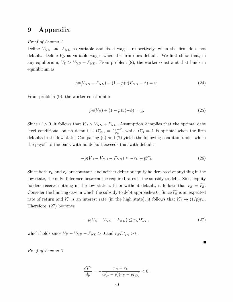
9 Appendix

Proof of Lemma 1

Define VND and FND as variable and fixed wages, respectively, when the firm does not

default. Define VD as variable wages when the firm does default. We first show that, in

any equilibrium, VD > VND + FND. From problem (8), the worker constraint that binds in

equilibrium is

pu(VND + FND) + (1− p)u(FND − φ) = u. (24)

From problem (9), the worker constraint is

pu(VD) + (1− p)u(−φ) = u. (25)

Since u′ > 0, it follows that VD > VND + FND. Assumption 2 implies that the optimal debt

level conditional on no default is D∗ND = rL−FrD

, while D∗D = 1 is optimal when the firm

defaults in the low state. Comparing (6) and (7) yields the following condition under which

the payoff to the bank with no default exceeds that with default:

−p(VD − VND − FND) ≤ −rE + prD. (26)

Since both rD and rE are constant, and neither debt nor equity holders receive anything in the

low state, the only difference between the required rates is the subsidy to debt. Since equity

holders receive nothing in the low state with or without default, it follows that rE = rE.

Consider the limiting case in which the subsidy to debt approaches 0. Since rE is an expected

rate of return and rD is an interest rate (in the high state), it follows that rD → (1/p)rE.

Therefore, (27) becomes

−p(VD − VND − FND) ≤ rED∗ND, (27)

which holds since VD − VND − FND > 0 and rED∗ND > 0.

Proof of Lemma 3

dF ∗

dp= − rE − rD

α(1− p)(rE − prD)< 0,

30

where the inequality follows from rE > rD.

dV ∗

dp=

rE − rDα(1− p)(rE − prD)

> 0,

where the inequality follows from rE > rD. It then follows that d(V ∗/F ∗)dp

> 0 since F ∗ > 0

and V ∗ > 0 by Assumption 3.

Proof of Lemma 4

We consider how all parameters change with F ∗, V ∗/F ∗, and D∗. The proof to Corollary 1

shows that dF ∗

dφ= 1 > 0, d(V ∗/F ∗)

dφ< 0, and dD∗

dφ< 0. The proof to Corollary 2 shows that

dF ∗

drD< 0, d(V ∗/F ∗)

drD< 0, and dD∗

drD> 0. The proof to Lemma 3 shows that dF ∗

dp< 0, d(V ∗/F ∗)

dp> 0.

Since D∗ = rL−F ∗

rD, it follows that dD∗

dp> 0. Next, it is trivial to see that dF ∗

dC> 0, d(V ∗/F ∗)

dC< 0

and, since D∗ = rL−F ∗

rD, it follows that dD∗

dC< 0. Now consider α:

dF ∗

dα= −

log( rE−prErE−prD

)

α2> 0 (28)

dV ∗

dα= −

log( rE−prDrD−prD

)

α2< 0, (29)

where the inequality in (28) follows since rE−prErE−prD

< 1, and the inequality in (29) follows sincerE−prDrD−prD

> 1. It follows that d(V ∗/F ∗)dα

< 0. Since D∗ = rL−F ∗

rD, it follows that dD∗

dα< 0. Next

consider rE:

dF ∗

drE= − prD

αrE(rE − prD)< 0 (30)

dV ∗

drE=

1

rE − prD> 0. (31)

It follows that d(V ∗/F ∗)dα

> 0. Since D∗ = rL−F ∗

rD, it follows that dD∗

drE> 0. Finally, F ∗ and V ∗

are independent of rL while it is trivial to see that D∗ is increasing in rL. It follows that, for

every parameter in V ∗ and F ∗, F ∗ is negatively correlated with D∗ and V ∗/F ∗ is positively

correlated with D∗.

Proof of Proposition 1

31

dD∗

dp=

dD∗

d(V ∗/F ∗)

d(V ∗/F ∗)

dp< 0, (32)

where the inequality follows from Lemma 3 and Lemma 4.

Proof of Corollary 1

Part 1: dV ∗

dφ= −1 < 0, dF ∗

dφ= 1 > 0; therefore d(V ∗/F ∗)

dφ< 0 since F ∗ > 0 and V ∗ > 0 by

Assumption 3.

Part 2: Since d(V ∗/F ∗)dφ

< 0 , Lemma 4 implies dD∗

dφ= dD

dVdVdφ< 0.

Proof of Corollary 2

Part 1: It is straightforward to show that dV ∗

drD> 0, dF ∗

drD< 0 and so d(V ∗/F ∗)

drD< 0 since V ∗ > 0

and F ∗ > 0 by Assumption 3.

Part 2: Since D∗ = rL−FrD

and both rD and F decrease, it is clear that debt increases.

Proof of Lemma 5

Let rNBD be the interest rate that a firm pays when there are no bankruptcy costs and

the firm defaults in the state L. rNBE is then the corresponding cost of equity.

(pH + pM + pL) (rL − F ) + rE

(1− rL − F

rD

)≥ (pH + pM) (rM − F ) + rNBE

(1− rM − F

rNBD

)(33)

The first terms on both sides of the above inequality are the payments to debt holders where,

for example, with no failure, the amount received by debt holders in all states is rL−FrD

rD.

Now consider the environment with bankruptcy costs. Comparing (22) with (21) and (22)

32

with (23) yields the following two conditions under which a firm chooses to default only in

state L:

(pH + pM)(rM − rL) ≤ pH(V ∗D1 − V ∗ND) + rE

(1− rL − F ∗ND

rD

)− rE

(1− rM − F ∗D1

rD

)(34)

pH(rD) ≥ pH(V ∗D1 − V ∗D2 + rM) + rE

(1− rM − F ∗D1

rD

). (35)

Where V ∗ND (F ∗ND) is the equilibrium variable (fixed) wage when the firm does not default,

V ∗D1 (F ∗D1) is the equilibrium variable (fixed wage) when the firm defaults in the low state.

Note that a fixed wage in this context is one that pays in the high and medium states only.

Finally, V ∗D2 is the variable wage if the firm defaults in both the medium and low states.

Note that no fixed wage can be paid in this case. To show that parameters exist such that

(34) and (35) can be satisfied, let pL → 0; thus rD → rNBD , rE → rNBE , rNBD → rD, rNBE → rE,

and it is straightforward to show that in equilibrium, V ∗D1 → V ∗ND. Using these, conditions

(34) and (33) collapse to the same inequality and so (34) must be satisfied. From (35) we

get

rD ≥ V ∗D1 − V ∗D2 + rM +rEpH

(1− rM − F ∗D1

rD

), (36)

which holds when the subsidy to debt is sufficiently small so that rD is sufficiently close to1pHrE.

33

References

Aldatmaz, S., P. Ouimet, and E. Van Wesep (2014). The option to quit: The effect of

employee stock options on turnover. CES working paper No. 14-06.

Allen, F., E. Carletti, and R. Marquez (2014). Deposits and bank capital structure. mimeo.

Bae, K.-H., J.-K. Kang, and J. Wing (2010). Employee treatment and firm leverage: A

test of the stakeholder theory of capital structure. Journal of Financial Economics 100,

130–153.

Berk, J., R. Stanton, and J. Zechner (2010). Human capital, bankruptcy, and capital

structure. Journal of Finance 65, 891–926.

Bertrand, M. and S. Mullainathan (2001). Are CEOs rewarded for luck? The ones without

principles are. The Quarterly Journal of Economics 116, 901 – 932.

Bewley, T. (1998). Why not cut pay? European Economic Review 42, 459 – 490.

Bronars, S. and D. Deere (1991). The threat of unionization, the use of debt, and the

preservation of shareholder wealth. The Quarterly Journal of Economics 106, 231 –

254.

Celerier, C. and B. Vallee (2015). Returns to talent and the finance wage premium. mimeo.

Crawford, A., C. Graham, and E. Bordeleau (2009). Regulatory constraints on leverage:

The Canadian experience. Bank of Canada Financial System Review (June).

Dasgupta, S. and K. Sengupta (1993). Sunk investment, bargaining and choice of capital

structure. International Economic Review 34, 203 – 220.

Diamond, D. and P. Dybvig (1983). Bank runs, deposit insurance, and liquidity. Journal

of Political Economy 91, 401 – 419.

Efing, M., H. Hau, P. Kampkotter, and J. Steinbrecher (2014). Incentive pay and bank risk-

taking: Evidence from Austrian, German, and Swiss banks. Journal of International

Economics 96, S123 – S140.

Fox, J. and V. Smeets (2011). Does input quality drive measured differences in firm pro-

ductivity? International Economic Review 42, 961 – 989.

Gopalan, R., T. Milbourn, and F. Song (2010). Strategic flexibility and the optimality of

pay for sector performance. The Review of Financial Studies 23, 2060 – 2098.

Gornall, W. and I. Strebulaev (2014). Financing as a supply chain: the capital structure

of banks and borrowers. Rock Center for Corporate Governance at Stanford working

paper No. 166.

34

Gorton, G. and A. Winton (2003). Financial intermediation. In G. Constantinides, M. Har-

ris, and R. Stulz (Eds.), Handbook of the Economics of Finance, Part A. Amsterdam:

North Holland.

Graham, J. (2000). How big are the tax benefits of debt? Journal of Finance 60, 1901 –

1942.

Griliches (1957). Specification bias in estimation of production functions. Journal of Farm

Economics 39, 8 – 20.

Gropp, R. and F. Heider (2010). The determinants of bank capital structure. Review of

Finance 14, 587–622.

Hall, B. and J. Liebman (1998). Are CEOs really paid like bureaucrats? Quarterly Journal

of Economics 111, 653 – 691.

Holmstrom, B. (1979). Moral hazard and observability. Bell Journal of Economics 10, 74

– 91.

Holmstrom, B. and J. Tirole (1997). Financial intermediation, loanable funds, and the

real sector. Quarterly Journal of Economics 112, 653 – 691.

Jacobson, L., R. Lalonde, and D. Sullivan (1994). Earnings losses of displaced workers.

American Economic Review 83, 685–709.

Jaggia, P. and A. Thakor (1994). Firm-specific human capital and optimal capital struc-

ture. International Economic Review 35, 283–308.

Jensen, M. and W. Meckling (1976). Theory of firm: managerial behaviour, agency costs

and capital structure. Journal of Financial Economics 3, 305–360.

Jensen, M. and K. Murphy (1990). Performance pay and top-management incentives.

Journal of Political Economy 98, 225 – 264.

Laffont, J.-G. and D. Martimort (2002). The Theory of Incentives: The Principal Agent

Model. Princeton University Press.

Lazear, E. and P. Oyer (2012). Personnel Economics. In R. Gibbons and D. J. Robert

(Eds.), Handbook of Organizational Economics, Chapter 13. Princeton University

Press.

Lemieux, T., W. Macleod, and D. Parent (2009). Performance pay and wage inequality.

Quarterly Journal of Economics 124, 1 – 49.

Lemmon, M., M. Roberts, and J. Zender (2008). Back to the beginning: Persistence and

the cross-section of corporate capital structure. Journal of Finance 63, 1575 – 1608.

35

Michelacci, C. and V. Quadrini (2008). Financial markets and wages. Review of Economic

Studies 76, 795 – 827.

Milbourn, T. (2003). CEO reputation and stock-based compensation. Journal of Financial

Economics 68, 233 – 262.

Morissette, R., X. Zhang, and M. Frenette (2007). Earnings losses of displaced workers:

Canadian evidence from a large administrative database on firm closures and mass

layoffs. Statistics Canada. Cat no. IIFOO19MIE - No. 291.

Morris, A. and W. Wilhelm (2007). Investment Banking: Institutions, Politics, and Law.

Oxford University Press.

Oyer, P. (2004). Why do firms use incentives that have no incentive effects? Journal of

Finance 4, 1619–1650.

Perotti, E. and K. Spier (1993). Capital structure as a bargaining tool: The role of leverage

in contract renegotiation. American Economic Review 83, 1131 – 1141.

Prendergast, C. (1999). The provision of incentives in firms. Journal of Economic Litera-

ture 37, 7 – 63.

Prendergast, C. (2000). What trade-off of risk and incentives? American Economic Re-

view 90, 421 – 425.

Simintzi, E., V. Vig, and P. Volpin (2014). Labor protection and leverage. Forthcoming

Review of Financial Studies.

Thanassoulis, J. (2012). The case for intervening in banker’s pay. Journal of Finance 67,

849–895.

36