Capital Markets Constrain Industry Scale

Eslyn L. Jean-Baptiste and Michael H. Riordan*

Columbia University

First draft: March 2003

This version: September 2003

Abstract

The paper considers an industry featuring agency problems between outside investors

and entrepreneurs who manage the firms comprising the industry. In a range of

circumstances, industry scale is independent of product market structure, and is

determined solely by the amount of equity financing contributed by the

entrepreneurs, and by the capital market’s response to possible managerial

malfeasance. Thus, in the face of capital market constraints, a change in product-

market concentration has no effect on market performance unless it occasions a

change in the amount of inside equity financing.

* We thank Judy Chevalier, Matt Rhodes-Kropf , seminar participants at Columbia Business School and the University of California at Berkeley, and participants at the 2003 NBER Corporate Finance Summer Institute for helpful comments on earlier versions.

1. Introduction

In their seminal article on the theory of the firm, Jensen and Meckling (1976)

recognized that the managers who control a firm can chose between consuming

perquisites (“non-pecuniary benefits”) and maximizing the value of the firm, and that the

agency costs of outside financing are determined jointly with the scale of the firm. We

build on these important observations to show how credit market constraints limit the

scale of an industry.

Jensen and Meckling’s (1976) analysis was at the level of the firm, not the

industry. They showed how the agency costs of outside equity reduced the optimal scale

of a firm. In contrast, we consider the interaction of capital and product market

competition, focusing on how default risk associated with managerial spending on

perquisites causes the credit market to ration firms participating in the same product

market. To be sure, Jensen and Meckling (1976, pp. 333-343) did recognize certain

costs of debt, but this was mainly to explain why outside financing does not consist

entirely of debt. In contrast, the main idea underlying our analysis is that managerial

spending on perquisites is potentially a source of default risk.

Our model of capital market and product market competition between

entrepreneurial firms yields an invariance result. Production by these firms is financed

by inside equity and debt. In a range of circumstances, industry scale is independent of

the number of competitors, and is determined solely by the capital market’s response to

possible managerial malfeasance and the amount of inside equity contributed by the

1 Williams (1995) is similar in spirit. In Williams' model, the capital market constraints that control managerial spending on perquistites distort an industry's choice of technology. In equilibrium, more firms adopt a high marginal cost technology, resulting in a smaller industry scale.

2

entrepreneurs who manage the firms. An additional competitor expands the market only

to the extent the entrepreneur who manages the new firm brings additional equity to the

industry. Thus, the degree of competition has a neutral effect on market performance,

unless the total amount of inside equity changes with the number of competitors in the

product market.

The idea that product market competition varies with the financial conditions of

firms has been demonstrated for a number of industries, including supermarkets

(Chevalier 1995a, 1995b; Chevalier and Scharfstein 1995, 1996) and airlines (Busse

2002). A leading theoretical explanation is the “limited liability effect” of capital

structure commitments on the equilibrium price and quantity strategies of firms (Brander

and Lewis 1986; Maksimovic 1988; Showalter 1995, 1996). An alternative possible

explanation is that the capital market controls managerial misappropriation by rationing

funds needed to finance production (Jensen and Meckling 1976; Bolton and Scharfstein

1990; and Albuquerque and Hopenhayn 2002). Our contribution is to develop the latter

argument at the level of the industry rather than just at the level of the individual firm.

We show that the equilibrium scale of an entrepreneurial industry depends on the extent

of its reliance on outside funds to finance production, and that the market share of an

individual firm depends both on its own financial condition and that of its rivals. Thus an

industry’s equilibrium competition in the product market is intertwined with its

competition in capital markets.1 We remark further on the relationship between our

theory and the received empirical and theoretical literatures as we go along.

Our approach departs from the conventional corporate finance wisdom that

product market competition disciplines firms and their managers. The informal

3

justification for this view is that competition fosters a form of natural selection that weeds

out incompetent, dishonest and imprudent managerial teams. Hart (1983) argues more

formally that competition reduces agency problems between managers and owners by

revealing more information, but this result is sensitive to assumptions about the

manager’s utility function (Scharfstein (1988)). Hermalin (1992) and Schmidt (1997) also

argue that the effect of competition on managerial incentives is ambiguous. Raith (2002)

develops a model in which shareholders provide managers with stronger incentives to

reduce costs when competition increases. Allen and Gale (2000) abstract from agency

problems, and argue that competition is more effective than standard corporate

government mechanisms at selecting more productive managerial teams. Our invariance

result is in stark contrast to these ideas, although admittedly we restrict our attention to

entrepreneurial firms.2 The invariance result of course also departs from the conventional

industrial organization wisdom.

The rest of our paper is organized as follows. The next section lays out our basic

assumptions about the structure of the product market and the capital market, and

establishes the optimality of simple debt contracts. Section 3 considers a monopoly

market structure, and shows how agency considerations cause the credit market to

constrain the scale of the firm below the neoclassical monopoly level. This section also

further discusses the relationship between our analysis and that of Jensen and Meckling

(1986). Section 4 generalizes the monopoly result to symmetric oligopoly, demonstrating

2 Jensen and Meckling (1976, p. 329) similarly distance their analysis from the then prevailing versions of this conventional wisdom: “It is frequently argued that the existence of competition in product (and factor) markets will constrain the behavior of managers to ideal value maximization, i.e., that monopoly in product (or monopsony in factor) markets will permit larger divergences from value maximization. Our analysis does not support this hypothesis. The owners of a firm with monopoly power have the same incentives to limit divergences of the manager from value maximization. (i.e. the ability to increase their wealth) as do the owners of competitive firms.”

4

how the capital market constrains the scale of the industry. This section derives our basic

invariance result: when capital market constraints are binding, equilibrium depends on

the total amount of industry inside equity, and not on the number of symmetric

competitors per se. The section also contrasts our analysis with Brander and Lewis

(1986). Section 5 extends the analysis to the case of asymmetric inside equity, and shows

that equilibrium industry scale depends on the total inside equity of credit-constrained

firms and the number of unconstrained firms. This section also relates our results to

some of the empirical literature on capital structure and product market competition.

Section 6 draws some policy conclusions. All proofs are presented in the Appendix.

2. Basic Economic Environment

Consider an economy in which only n entrepreneurs can sell a unique product,

either because they each have a well-defined property right over the relevant production

technologies, or because only they have the required managerial talent to run the

production processes.3 The market has the following structure. The production

technologies exhibit constant returns to scale, and the average cost of production is equal

to c. Inputs must be purchased in advance of production, and the opportunity cost of a

unit of financial capital is ( )1 r+ . Revenue is a function of the quantity of output,

( ) ( )R Q P Q Q= , where ( )P Q is the (inverse) demand curve. The demand curve is

downward sloping and continuous, as is the corresponding marginal revenue curve.

Moreover, (0) 0R = and '(0) (1 )R r c> + .

3 For example, FCC licensing of spectrum rights limits the number of competitors in markets for wireless telephony.

5

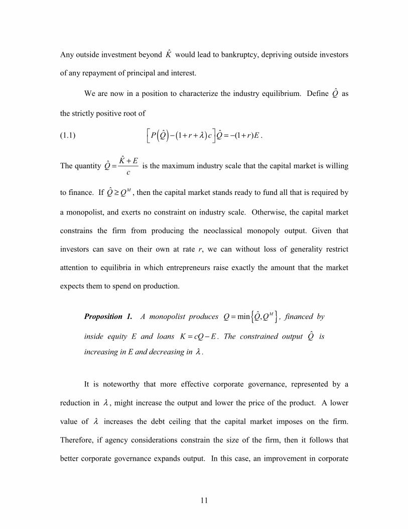
We are interested in exploring how the credit market might constrain the product

market outcome. Toward this end we assume that the entrepreneur is endowed with a

limited amount of financial capital, ie and denote the total amount of “inside” capital in

the industry as 1

n

ii

E e=

=∑ . The entrepreneurs invest these amounts in their respective

enterprises, but must raise additional funds on the capital market in order to expand

industry production beyond Ec

. In order to produce quantity ii

eqc

> , an entrepreneur

must raise a sufficient amount of financial capital, i i ik cq e≥ − , from outside investors.

The capital market is perfectly competitive, and outside investors are willing to lend

funds at an interest rate of r when there is no default risk. Loans are repaid at the end of

the period.

The agency problem for outside investors is that each entrepreneur has the ability

to divert funds to non-productive managerial perquisites. More precisely, the

entrepreneur can spend each dollar of financial capital either on production or on

perquisites with a monetary-equivalent value of λ (measured at the end of the period).

λ is commonly known to all agents. In addition, we assume that 0 1 rλ< < + , which

means that it would be inefficient for outside investors to fund managerial perquisites.

The problem facing investors is that managerial spending on perquisites is not verifiable,

and cannot be recovered if the entrepreneur/manager defaults on the loan and enters

bankruptcy.4 Therefore, investors are concerned about expropriation by managerial

malfeasance.

4 Default and bankruptcy are synonymous in our model. The important idea is that bankruptcy effectively shields entrepreneurs from the claims of lenders. In our simple model, there are no assets to liquidate in bankruptcy, so default means simply that creditors are not repaid.

6

The market unfolds in two stages. At stage 1, the capital market supplies

financial capital (1

n

ii

K k=

=∑ ) that augments the entrepreneurs’ initial investment of equity

(E). At stage 2, the entrepreneurs allocate available financial capital between productive

inputs and managerial perquisites; any remaining funds are kept as reserves and invested

at the prevailing rate r. Capital markets have rational expectations and at stage 1, supply

funds up to the point of zero expected profits given rational expectations about the

entrepreneurs’ (monetary-equivalent) utility-maximizing decisions at stage 2. These two

conditions, utility-maximizing production and the capital-market competition, define

industry equilibrium.

We emphasize our twin assumptions that, while production decisions and the

related expenditures are not contractible, their outcomes are; that is revenues from

production (and cash reserves) are verifiable and contractible. These assumptions capture

the stylized facts that production decisions are a managerial prerogative precisely because

these decisions are complex and require expertise. Managers can take advantage of the

opacity of the firm’s operations to outsiders and of the discretion that they enjoy over the

use of the firm’s resources to divert these resources instead of using them for productive

purposes.5 Thus managerial “stealing” is the process of transforming financial capital into

private benefits or assets that cannot be verified or recovered by investors and courts.

Because managers have limited liability and cannot be punished beyond the verifiable

amount of the firm’s income, this creates a moral hazard problem. When managers

actually engage in production and do not steal, however, the resulting income can be 5 In practice some operating expenditures are verifiable and most firms invest in plants and other assets that are sometimes used as collateral. However, as long as the operations of the firm require substantial investments in other assets that can be transferred (e.g. working capital) or are intangible (e.g. R&D), the qualitative results of the model will hold.

7

verified and recovered by debt-holders (as in Townsend (1979)). This is consistent with

the fact that legal claims against sales receipts are usually enforceable in bankruptcy.

There is no role for outside equity in our model. The substitution of outside

equity for debt would only increase an entrepreneur’s incentive to divert capital spending

to perquisites.6 Thus, the “capital market” is synonymous with the “credit market”, and

we restrict our attention to debt contracts as means of outside finance. A proof that this

restriction does not entail any loss of generality is presented in the Appendix.

Lemma. Simple debt contracts are optimal.

3. Monopoly

The monopoly case (n=1) provides initial insights into how the capital market

constrains production decisions. Neoclassical monopoly profit is given by

( ) ( ) (1 )W Q P Q Q r cQ= − +

Our assumptions imply that the neoclassical monopoly output, QM, is positive and

satisfies the first-order condition for profit-maximization, '( ) (1 )MR Q r c= + . We want to

explore how the credit market might reduce equilibrium output below the monopoly

level. Toward this end we assume that the entrepreneur is endowed with a limited

amount of financial capital, ME cQ< .

Figure 1 illustrates the industry equilibrium for the case in which the capital

market constrains output below the neoclassical monopoly level. The concave curve is

6 Jensen and Meckling (1976, pp. 330-343) recognize this point, and get around it by introducing additional agency costs of debt. We ignored these additional considerations in order to simplify and focus on our main idea that capital markets deal with agency costs by constraining industry size.

8

the neoclssical monopoly profit and the upward sloping line is the maximum net benefit

from diverting financial capital from production to perquisites. The equilibrium output is

Q̂ , which is less than the neoclassical monopoly output MQ . The crucial feature of this

construction is that the two curves intersect at Q̂ , indicating that, in the equilibrium, the

entrepreneur is just indifferent between production and perquisites. If the capital market

were to lend additional funds, then, as we show below, the entrepreneur would have an

incentive to spend everything on perquisites and default on the debt.

Figure 1 also makes clear that our results do not depend crucially on the linearity

of the stealing technology. As long as the curve representing the benefits of stealing is not

too concave and cuts the neoclassical profit curve from below, our conclusions are

unaffected.

We now analyze the industry equilibrium more carefully. We begin by analyzing

the entrepreneur’s production decision given financial resources ( )K E+ , where K is

debt and E is inside equity. The entrepreneur can invest some of its financial capital cQ

in production to generate end of period revenues ( )R Q , save an amount I as reserve and

earn (1 )I r+ and squander the rest of the funds on perquisites and obtain a private benefit

equal to ( )E K cQ Iλ + − − . Any claims are paid out of revenues and reserves since

spending on perquisites cannot be recovered in bankruptcy. Therefore, the entrepreneur’s

choice problem is:

( ) ( ) ( ),

, , (1 ) 1 ( )Q I

Max Q E K P Q Q r I r K E K cQ Iπ λ+= + + − + + + − −

subject to I cQ E K+ ≤ + 0I ≥ 0Q ≥

9

In the statement of this problem, the notation [ ] { }max ,0X X+� recognizes the limited

liability of the entrepreneur.

Two observations shed light on how the solution of this problem departs from the

standard marginal analysis. First, it is never optimal for the entrepreneur to choose

positive levels of production and reserves that are insufficient to pay the debt fully. The

reason for this is that the entrepreneur is always better off “stealing” these funds (i.e.

diverting these funds to perquisites). Second, it is never optimal for the entrepreneur to

steal some funds while producing and saving enough to repay the debt in full. The

intuition for this is that the entrepreneur is in effect stealing from himself when debt is

repaid in full. Since stealing is inefficient, this behavior is suboptimal. These two facts

imply that stealing is an all or nothing proposition for the entrepreneur, and that, in

equilibrium, stealing cannot coexist with strictly positive output.7

Thus the entrepreneur makes a binary decision between investing in perquisites

and investing in production.8 The entrepreneur elects to spend financial capital on

production if and only if I cQ E K+ = + and ( , , ) ( )Q E K E Kπ λ≥ + for some

0 E KQc+< ≤ . These expressions combine to imply the following incentive-

compatibility constraint

7 Another way to understand the entrepreneur’s decision is to recognize the option-like structure of her levered equity. The entrepreneur must choose between “legitimate” compensation through productive behavior and “illegitimate” gains through stealing. However, the legitimate rewards are obtained only if the debt is repaid in full. Once debt is repaid, all the surplus goes to the entrepreneur. Therefore conditional on repaying the debt, the entrepreneur will always behave efficiently and avoid stealing; her option is “in the money”. However, when debt is expected not to be repaid in full (the option is out of the money), the entrepreneur cannot get any legitimate rewards and so her best strategy is to get the maximum illegitimate rewards and steal everything. 8 This is due to the assumption that stealing is inefficient. Relaxing this assumption would not change the flavor of our results. More on this below.

10

( ) ( ) (1 )W Q E K r Eλ≥ + − + for 0 E KQc+< ≤ .

The left-hand side of the inequality is the total production surplus available to the

entrepreneur. The right-hand side is the premium the entrepreneur obtains from the

monetary-equivalent value of perquisites. Thus, this is a “no-stealing constraint”; the

entrepreneur has no incentive to divert working capital to perquisites.

The monopolist never produces more than MQ because beyond the neoclassical

monopoly output the marginal revenue of an additional dollar invested in production is

lower than (1+r) and this is always dominated by saving when output is positive (and

debt is fully repaid). Also, if ME K cQ+ < , and the entrepreneur produces at all, then she

invests all her capital in production; that is, the entrepreneur never chooses a quantity

0 max , ME KQ Qc+ < <

. The reason for this is that, because quantity is positive, there

is no stealing, and any amount not used in production is saved as reserve; however, the

reserve only generates (1+r) when production an extra dollar invested in production

generates ( ) (1 )R Q rc

′> + . In other words, the firm produces

( , ) min , ME KQ E K Qc+ =

, if this value satisfies the above incentive-compatibility

constraint, and produces 0Q = otherwise.

The capital market anticipates the behavior of the entrepreneur and will provide

funds up to K̂ satisfying

( )ˆ ˆ ˆ(1 )( ) 1E K E KP r E K r E

c cλ

+ + − + + + = − +

.

11

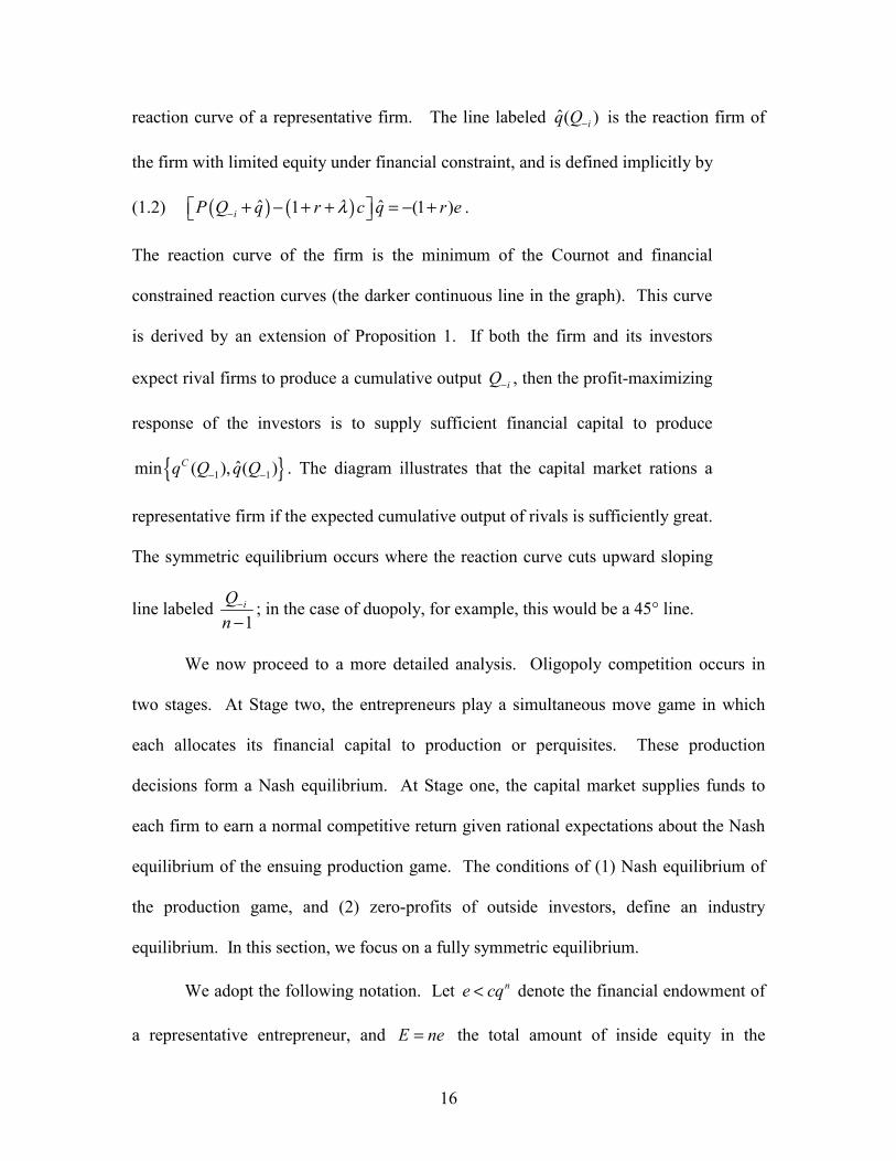
Any outside investment beyond K̂ would lead to bankruptcy, depriving outside investors

of any repayment of principal and interest.

We are now in a position to characterize the industry equilibrium. Define Q̂ as

the strictly positive root of

(1.1) ( ) ( )ˆ ˆ1 (1 )P Q r c Q r Eλ − + + = − +

.

The quantity ˆˆ K EQ

c+= is the maximum industry scale that the capital market is willing

to finance. If ˆ MQ Q≥ , then the capital market stands ready to fund all that is required by

a monopolist, and exerts no constraint on industry scale. Otherwise, the capital market

constrains the firm from producing the neoclassical monopoly output. Given that

investors can save on their own at rate r, we can without loss of generality restrict

attention to equilibria in which entrepreneurs raise exactly the amount that the market

expects them to spend on production.

Proposition 1. A monopolist produces { }ˆmin , MQ Q Q= , financed by

inside equity E and loans K cQ E= − . The constrained output Q̂ is

increasing in E and decreasing in λ .

It is noteworthy that more effective corporate governance, represented by a

reduction in λ , might increase the output and lower the price of the product. A lower

value of λ increases the debt ceiling that the capital market imposes on the firm.

Therefore, if agency considerations constrain the size of the firm, then it follows that

better corporate governance expands output. In this case, an improvement in corporate

12

governance, that lessens a manager’s ability to benefit from wasteful non-pecuniary

consumption, improves social welfare.

It is also noteworthy that an increase in the amount of equity capital supplied by

entrepreneur might expand output. The fact that Q̂ is increasing in E means that the

capital market is willing to fund a larger scale of production if the entrepreneur/manager

has a greater amount of equity capital at stake.9

The fact that there is never any stealing in equilibrium is a direct consequence of

the assumption that stealing is inefficient, i.e. 1 rλ < + . Relaxing this assumption would

not change the flavor of the proposition but would generate equilibrium stealing as is

illustrated in the Appendix. However, this assumption is useful because it allows us to

focus on the product-market effects of credit-market constraints, rather than on the

amount of equilibrium stealing. The latter element is, in our view, the more obvious but

less important manifestation of agency costs.

We illustrate the proposition with the simple example of a linear inverse demand

function of the form ( )P Q A Q= − . It is straightforward to verify that the monopoly

output is given by (1 )2

M A r cQ − += . The parametric restriction ( )1A r c≥ + is necessary

for production to occur ever. The minimum level of inside equity ME that can support the

monopoly output is given by replacing Q̂ by the value for MQ in (1.1)

( ) ( )1 2 14(1 )

M A r c A r cE

rλ

+ − + + − + = −

+ .

9 Whether or not the amount of industry debt ( Q̂ E− ) increases with E is ambiguous.

13

If parameters are such that ( )1 2A r cλ≥ + + , then 0ME = , and the monopoly output

obtains even when the entrepreneur is penniless. The resulting equilibrium can be written

as:

( ) ( )( )*

2

(1 )2

1ˆ 1 [ 1 ] 4(1 )2

M M

M

A r cQ if E EQ

Q A r c A r c r E if E Eλ λ

− + = ≥= = − + + + − + + + + <

.

Note also that when capital market imperfections constrain output below the monopoly

level, that is, when ME E< (or equivalently when ˆ MQ Q< ), the equilibrium output

increases with the amount of inside equity.

Inside equity capital is also important for understanding industry growth in a

dynamic monopoly model. In the Appendix we add an additional production period to

the monopoly model, and show that this relaxes the capital market incentive

compatibility constraint. The option to produce and earn a monopoly rent in the second

period effectively reduces the entrepreneur’s incentive to steal in the first period,

assuming that the entrepreneur losses her property right in the event of bankruptcy.

Moreover, retained profits from the first period contribute inside equity capital in the

second period. The spirit of our two-period analysis is similar to Albuquerque and

Hopenhayn (2002) who consider a richer dynamic model of a credit-constrained

entrepreneurial firm.10

A discussion of the relationship between this analysis and the one in Jensen and

Meckling (1976) also is presented in the Appendix. The main differences are that our 10 The Albuquerque and Hopenhayn (2002) model features an infinite horizon, demand uncertainty, and a more general “stealing” technology. The optimal debt contract does not have a simple structure; indeed, once the firm grows to optimal size, the entrepreneur is paid a fixed dividend and the “lender” becomes a residual claimant. Before this point, however, the entrepreneur receives nothing, i.e. all accumulated “inside equity” is reinvested in the firm, as in our model.

14

model (i) assumes that perquisites are inefficient, and (ii) allows for the possibility of

default (and bankruptcy) caused by managerial spending on perquisites. We have shown

that, if the capital market were to provide enough financial capital to achieve a monopoly

scale, then the entrepreneur who manages the firm might choose to spend these resources

on perquisites, produce nothing, and declare bankruptcy. This case occurs when

monopoly rents are small relative to the value of perquisites. In this case, the capital

market responds by reducing the amount of financial capital available to the firm, thus

reducing scale below the monopoly level.

4. Symmetric Oligopoly

We now consider competition between n ≥ 2 symmetric firms who compete in the

product market and also compete for funds in the capital market. Barriers to entry into

the product market are absolute.

The product market has the same structure as before except for the number of

market participants. The market demand curve and marginal revenue curve are

downward sloping and continuous, and all firms possess the same constant returns

production technology. Inputs are purchased in advance of production, and the capital

market is competitive.

The symmetric Cournot equilibrium is a benchmark. This Cournot solution has

an industry output n nQ nq= satisfying

( ) ( )' 1n n nP Q q P Q r+ = + .

15

nQ is non-decreasing in n. A sufficient condition for a unique and symetric Cournot

equilibrium is that P(Q) is log-concave (Amir and Lambson, 2000). Let ( )Ciq Q−

represent the Cournot best response function for a representative firm (Firm i) when

competitors produce Q-i.

We consider how agency problems can result in an industry scale below the

Cournot level. Toward this end, we assume that each firm is owned and managed by an

entrepreneur with limited equity capital, and uses debt financing to expand production.

The agency problem is that each entrepreneur can spend these funds on non-productive

managerial perquisites, receiving a proportional private benefit. Therefore, as in the

monopoly case, the capital market advances funds to firms in this industry only if an

appropriate incentive compatibility constraint holds. The constraint assures outside

investors that the entrepreneurs have incentives to allocate financial capital to production

rather than to perquisites. We show that the capital-market incentive-compatibility

constraint on symmetric entrepreneurial firms competing in a Cournot product market

can constrain industry scale. Cournot interaction in the product markets is a very natural

framework for our analysis of equilibrium industry capacity. Indeed, the main point of

the paper is that because firms must acquire capacity first before engaging in production,

they need to convince capital markets to finance these investments in capacity. The need

for capacity commitment, is a feature that is also emphasized in the setting of Kreps and

Scheinkman (1983) who show that Bertrand competition yields Cournot outcomes .

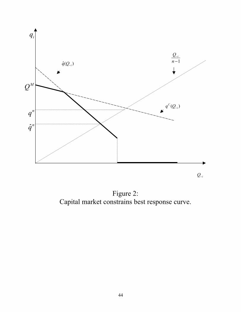
A symmetric oligopoly equilibrium for a financially constrained industry is

illustrated Figure 2. The downward-sloping line labeled ( )Ciq Q− is the standard Cournot

16

reaction curve of a representative firm. The line labeled ˆ( )iq Q− is the reaction firm of

the firm with limited equity under financial constraint, and is defined implicitly by

(1.2) ( ) ( )ˆ ˆ1 (1 )iP Q q r c q r eλ− + − + + = − + .

The reaction curve of the firm is the minimum of the Cournot and financial

constrained reaction curves (the darker continuous line in the graph). This curve

is derived by an extension of Proposition 1. If both the firm and its investors

expect rival firms to produce a cumulative output iQ− , then the profit-maximizing

response of the investors is to supply sufficient financial capital to produce

{ }1 1ˆmin ( ), ( )Cq Q q Q− − . The diagram illustrates that the capital market rations a

representative firm if the expected cumulative output of rivals is sufficiently great.

The symmetric equilibrium occurs where the reaction curve cuts upward sloping

line labeled 1iQ

n−

−; in the case of duopoly, for example, this would be a 45° line.

We now proceed to a more detailed analysis. Oligopoly competition occurs in

two stages. At Stage two, the entrepreneurs play a simultaneous move game in which

each allocates its financial capital to production or perquisites. These production

decisions form a Nash equilibrium. At Stage one, the capital market supplies funds to

each firm to earn a normal competitive return given rational expectations about the Nash

equilibrium of the ensuing production game. The conditions of (1) Nash equilibrium of

the production game, and (2) zero-profits of outside investors, define an industry

equilibrium. In this section, we focus on a fully symmetric equilibrium.

We adopt the following notation. Let ne cq< denote the financial endowment of

a representative entrepreneur, and E ne= the total amount of inside equity in the

17

industry. Similarly, let K nk= denote amount of industry debt that is raised on the

capital market. If financial capital is fully invested in production, then industry output is

( )n e kQ nqc+= = .

Analysis of the production game is crucial for understanding capital market

equilibrium. Consider the reaction function of Firm i. Suppose that the firm has

borrowed ki, and expects its rival to produce a quantity of output Q-i. The choice problem

confronting the entrepreneur/manager of Firm i is:

( ) ( ) ( ),

, , (1 ) 1 ( )i i

i i i i i i i i i i iq IMax q e k P Q q q r I r k e k cq Iπ λ+

−= + + + − + + + − −

subject to i i iI cq e k+ ≤ + 0iI ≥ 0iq ≥

where iI is the amount of financial capital the firm holds in cash reserves.

The similarities with the monopolist’s production problem are obvious, and

similar arguments to the monopoly analysis yield two conclusions. First, the rational

entrepreneur elects to produce a positive quantity 0 ii

e kqc+< ≤ if and only if this

quantity satisfies the incentive-compatibility constraint

( )( ; ) (1 ) ( ) (1 )i i i i i i iw q Q P Q q q r cq e k r eλ− −= + − + ≥ + − + ,

where the left-hand side is the surplus from production available to the entrepreneur and

the right-hand side is the perquisite premium. Second, the entrepreneur never produces

more than her Cournot best reply, i.e. ( )ci iq q Q−≤ , and may produce strictly less is

financial capital is insufficient. Thus, in reaction to Q-i , the firm produces the quantity

( ; , ) min , ( )cii i i i

e kq Q e k q Qc− −+ =

if this quantity satisfies the above incentive-

18

compatibility constraint, and produces 0iq = otherwise. Because the Cournot reaction

curve ( )ni iq Q− is non-increasing, Firm i's reaction curve at Stage 2 is a discontinuous

function of the form

( ; , ) ( , )

( ; , )0 ( , )

i i i i i ii i i

i i i

q Q e k if Q Q e kq Q e k

if Q Q e k− − −

−− −

≤= >

where ( , )i iQ e k− is defined by the binding incentive-compatibility constraint

( )( ); ( ) (1 )i i i iw q Q Q e k r eλ− − = + − + .

Thus, limited financial capital and the opportunity to consume perquisites modify the

firm’s best-response curve. It follows from these conclusions that, for an arbitrary

subgame (defined by ik , i = 1,…n), the equilibrium production profile *( )iq , satisfies

either * *( , ) ( ; , )i i i i iq e k q Q e k−= , in which case Firm i's incentive-compatibility constraint

holds, or *( , ) 0i iq e k = and the constraint fails.11

Given the capital market’s rational expectations, investors never finance a firm

when they expect the entrepreneur to steal resources. Satisfaction of the capital market

incentive compatibility constraint implies that there is no diversion of funds to

perquisites, and, because investors can save on their own, we safely can restrict attention

to equilibria in which capital markets provide funds only when they expect all the firm’s

capital to be used on production, that is when ii

e kqc+= . If i

ie kq

c+< , then marginal

investors could just as well withdraw their investment in the firm.

11 The equilibrium of that subgame is not necessarily unique since there could exist several equilibria of the subgame in which one or more players produce nothing and steal all the funds.

19

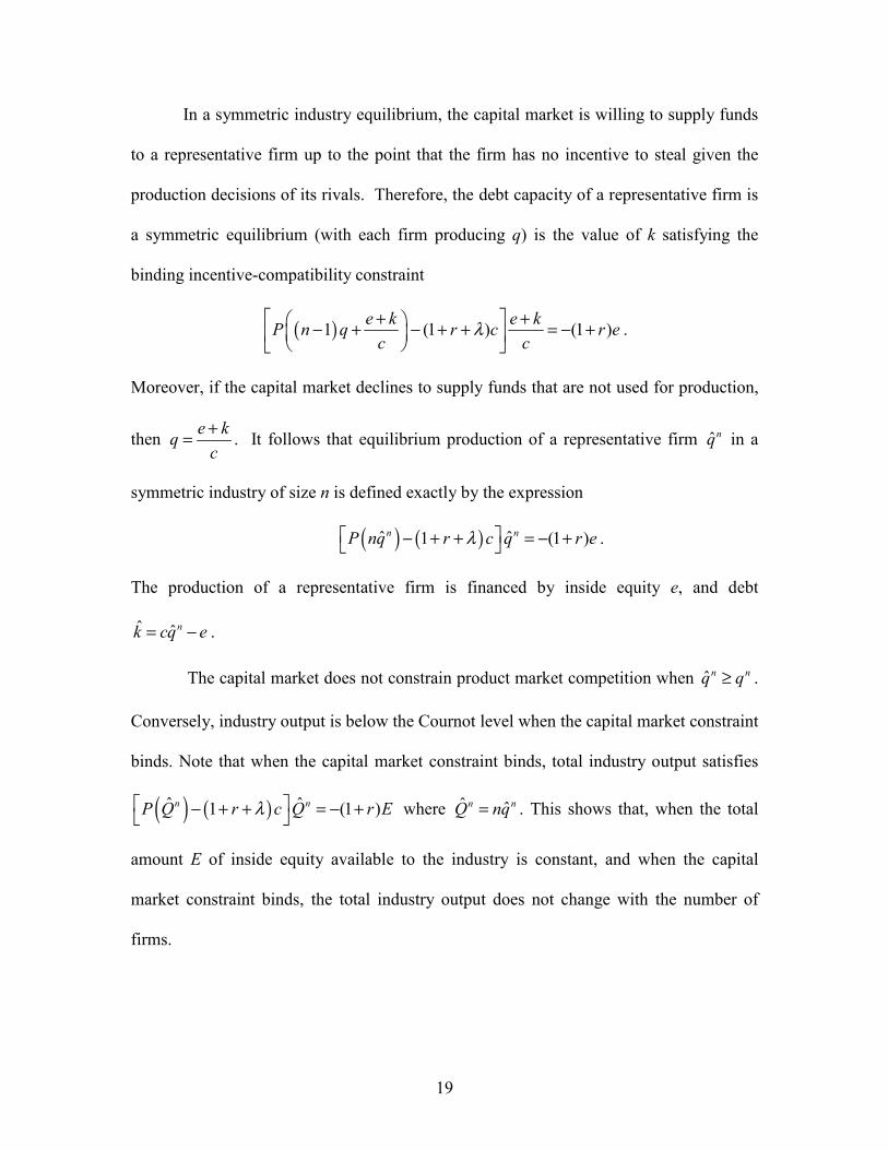
In a symmetric industry equilibrium, the capital market is willing to supply funds

to a representative firm up to the point that the firm has no incentive to steal given the

production decisions of its rivals. Therefore, the debt capacity of a representative firm is

a symmetric equilibrium (with each firm producing q) is the value of k satisfying the

binding incentive-compatibility constraint

( )1 (1 ) (1 )e k e kP n q r c r ec c

λ + � + �− + − + + = − + � � �

.

Moreover, if the capital market declines to supply funds that are not used for production,

then e kqc+= . It follows that equilibrium production of a representative firm ˆnq in a

symmetric industry of size n is defined exactly by the expression

( ) ( )ˆ ˆ1 (1 )n nP nq r c q r eλ − + + = − + .

The production of a representative firm is financed by inside equity e, and debt

ˆ ˆnk cq e= − .

The capital market does not constrain product market competition when ˆn nq q≥ .

Conversely, industry output is below the Cournot level when the capital market constraint

binds. Note that when the capital market constraint binds, total industry output satisfies

( ) ( )ˆ ˆ1 (1 )n nP Q r c Q r Eλ − + + = − +

where ˆ ˆn nQ nq= . This shows that, when the total

amount E of inside equity available to the industry is constant, and when the capital

market constraint binds, the total industry output does not change with the number of

firms.

20

Proposition 2. In a symmetric oligopoly, there is a unique

symmetric equilibrium in which each firm produces { }ˆmin ,n nq q q= ,

financed by inside equity e and loans k cq e= − . The constrained output

ˆnq is increasing in e and decreasing in λ. Furthermore, if the capital

market constraint binds for n entrepreneurs (i.e. ˆn nq q< ), then it also

binds for (n+1), holding the total amount of industry inside equity

constant, and total industry output therefore does not change with an

increase in the number of firms.

It is remarkable that the industry scale can be invariant to market concentration.

While the standard Cournot industry output strictly increases in the number of active

firms (Amir and Lambson, 2000), the financially-constrained industry output does not

depend on n. That is, if ˆMQ Q> , then n MQ Q> , and industry scale is invariant to

market concentration in a symmetric equilibrium (keeping total inside equity E constant

and adjusting each individual firm’s inside equity to the level Een

= ). When industry

output is not constrained by the agency problem confronting entrepreneurs and outside

investors, each firm produces the symmetric Cournot output, and an increase the number

of firms expands the scale of the industry.

Note that capital market constraint necessarily binds as the industry becomes less

concentrated holding industry inside equity constant. The perfectly competitive output

level *Q satisfies

*( ) (1 )P Q r c= + .

21

While the Cournot output converges to *Q as n → ∞ , the equilibrium output of a

financially-constrained industry remains at a scale *Q̂ Q< .

Similarly to the monopoly model, an increase in the amount of inside equity

supplied by entrepreneurs might expand industry scale. New entry expands the market

only to the extent that the new entrant contributes additional inside equity to the industry.

New entrants that rely more heavily on debt than inside equity exert less competitive

pressure on the product market.

Also as in the monopoly model, an improvement in industry-wide corporate

governance improves social welfare by expanding the market. We have argued that

agency problems can cause credit markets to limit the scale of an industry. An interesting

corollary of this general point is that private parties should not be expected to invest

optimally in corporate governance. The benefits of market expansion accrue partly to

consumer welfare that would not be internalized by entrepreneurs when organizing their

firms. From this perspective, a public policy toward corporate governance could be as

important as antitrust policy for increasing social welfare.

We now illustrate our analysis of symmetric oligopoly with the linear demand

example from above. When the demand function is linear, the standard Cournot output is

given by (1 )1

n A r cqn

− +=+

. This equilibrium can be supported only if each entrepreneur’s

inside equity satisfies the condition ( )

2

1 ( 1) [ (1 ) ](1 )( 1)

n A r n c A r ce e

r nλ

+ − + + + − + ≥ = −

+ + .

This expression shows that when n is small enough (that is (1 )A r cnc

λλ

− + +≤ ) the

unique and symmetric Cournot equilibrium can be supported with zero inside equity. As

22

in the monopoly case this is possible only if parameters are such that (1 )A r cλ≥ + + .

Furthermore, when [ ]2 (1 )1

A r cn

cλ− +

≥ − we have 0nde

dn≤ .

However, when inside equity is low enough (that is ne e< ), the unique

equilibrium output is ( ) ( )( )21ˆ 1 [ 1 ] 4 (1 )2

nq A r c A r c n r en

λ λ= − + + + − + + + + . Note

that in this case ˆ

0nq

e∂ >∂

and ˆ

0nq

λ∂ >∂

. Replacing ne by E in the expression for ˆnq , it is

clear that the expression ˆnnq is independent of n when E is constant.

In order to illustrate the effect of capital market constraints on the outcome of

product market competition, consider the case of splitting a constrained monopolist into

two identical firms. According to the above analysis, a monopolist is constrained if

parameters are such that ( ) ( )1 2 1

4(1 )M A r c A r c

E Er

λ+

− + + − + < = − +

and

( ) ( )1 1 2r c A r cλ+ ≤ < + + . Suppose that the monopoly firm is split into two identical

firms each with equity 2Ee = . This split changes total equilibrium output from the

constrained monopoly level ( ) ( )( )21ˆ 1 [ 1 ] 4(1 )2

MQ A r c A r c r Eλ λ= − + + + − + + + + to

the constrained duopoly output

( ) ( )( )21ˆ ˆ2 1 [ 1 ] 4(1 )2

D DQ q A r c A r c r Eλ λ= = − + + + − + + + + , that is total output does

not change at all.

We close this section by comparing our analysis of symmetric oligopoly with

Brander and Lewis (1986). Brander and Lewis identified the “limited liability effect” of

23

debt, namely, that increased debt encourages managers to expand production in order to

increase profits in high-demand and low-cost states of the world in which the firm

remains solvent. No such effect appears in our model. There are several differences

between our model of symmetric oligopoly and the Brander-Lewis model explaining this.

First, and most importantly, managers have the option of spending working capital on

perquisites. Secondly, the firm is equity-constrained, i.e. entrepreneurs contribute a

limited amount of financial capital, and there is no role for outside equity. Third, and

least importantly, there is no product market uncertainty. Product market uncertainty is

key ingredient of the Brander-Lewis limited liability effect, but it is not a sufficient

ingredient. Nothing important would change if we were to introduce product market

uncertainty into our model of a capital-constrained industry. The capital market would

still ration firms in order to prevent the misappropriation of working capital, and the firm

would be unable to expand production because of its financial constraints. The only

difference is that firms’ output level would be constrained below the Brander-Lewis

equilibrium level rather than the Cournot level. Thus, if our model were extended to

product market uncertainty, the limited liability effect would reappear under certain

conditions even in a capital-constrained industry. If the capital-market constraint were

slack, however, then the limited liability effect identified by Brander and Lewis (1988)

would determine the equilibrium level of output.. In this way our model lays the

groundwork for a more general framework with richer empirical predictions.

5. Asymmetric equity

24

We now allow that the otherwise symmetric entrepreneurs supply different

amounts of equity capital. We show that industry scale still depends on the total amount

of inside equity of constrained firms, and when all firms are constrained, a firm’s share of

the product market is equal to its share of industry inside equity.

Suppose Firm i has equity capital cie cq< , has borrowed ki, and expects its rivals

to produce a cumulative quantity Q-i. A similar analysis to the symmetric case allows us

to conclude that the firm’s best response is a discontinuous function: the entrepreneur

produces ( ; , ) ( , , )i i i i i i i iq Q e k q Q e k− −= if and only if i iQ Q− −≤ (where iQ− is defined by

( )( ); ( ) (1 )i i i i i iW q Q Q e k r eλ− − = + − + as in the symmetric case) and nothing otherwise.

The capital market anticipates these incentives and advances funds to each firm

up the point at which the incentive-compatibility constraint binds, that is

( )(1 ) 1i i i ii i

e k e kP Q r c r ec c

λ− + � + �+ − + + = − + � �

�. Given the investors’ rational

expectations and their ability to invest on their own at rate r, we can restrict our attention

to equilibria in which each firm is expected to invest all its funds in production, that is

i ii

e kqc+= . It is straightforward to verify that in equilibrium there can be only two types

of firms. One subset of firms are constrained by agency problems and therefore are not

producing the Cournot best response to their competitors’ output; i.e. their output is

characterized by ( , ) ( )ni i i i iq e k q Q−< and ( ) ( )(1 ) 1i i i iP Q q r c q r eλ− + − + + = − + . The

other set of firms are unconstrained by the capital market and are on their Cournot best

response curves; i.e. ( ; , ) ( )ni i i i i iq Q e k q Q− −= and

25

( )(1 ) 1i i i ii i

e k e kP Q r c r ec c

λ− + � + �+ − + + ≥ − + � �

�. Equilibrium is described by the

following proposition.

Proposition 3. With an asymmetric allocation of inside equity,

equilibrium is essentially unique12 and can be characterized as follows.

Some firms are unconstrained and produce the Cournot best response to

their competitors’ output while others are constrained and produce less

than their best response. Furthermore, all unconstrained firms produce

the same quantity of output and have higher levels of equity and output

than the constrained firms. The debt and output levels of the constrained

firms are proportional to the amount of their contributions of inside

equity. Finally, splitting a constrained firm into smaller firms does not

change total industry output.

Naturally, the unconstrained firms are those with more equity. These firms are on

their Cournot best response curves, and it is no matter whether they finance production

with debt or equity as long as their capital market constraints remain slack (Modigliani

and Miller (1958)). Among the subset of constrained firms, those with more equity are

able to borrow more and have a larger market share. All constrained firms are equally

leveraged (i.e. have the same debt-equity ratio), while unconstrained firms are less

leveraged than their constrained competitors.

12 Equilibrium outputs of all firms and the capital structure of constrained firms is unique. As discussed below, there is an inconsequential indeterminancy in the capital structure of unconstrained firm.

26

Increasing the amount of equity financing of an unconstrained firm has no effect

on equilibrium output. However, this is not true for constrained firms and an increase in

the equity of these firms does increase output. Similarly, splitting a constrained firm into

separate firms does not change the total level of output; the output of the original firm is

just split between the spin-offs proportionally to the split of equity. In contrast, splitting

an unconstrained firm or reallocating equity from constrained to unconstrained firms can

affect equilibrium output.

It is interesting to consider the bilateral incentives to merger in our model. If a

credit-constrained firm acquires a competitor, and finances the acquisition with debt, then

industry output decreases and the product price rises to the extent that the merger reduces

industry inside equity. This capital market response to a horizontal merger is not

discussed in the Horizontal Merger Guidelines published by the U.S. Department of

Justice. Such a consideration also is absent from Salant, Switzer, and Reynolds’ (1983)

classic analysis of bilateral merger incentives for the standard Cournot model. A

bilateral merger might be profitable in our model, when it is not profitable in the standard

model, if capital market constraints reduce the ability of rival firms to expand in response

to an increase in product price.

We close this section by relating our results to some relevant empirical literature.

Various empirical studies establish a link between product market behavior and financial

conditions. For instance, Chevalier (1995a) documents that the leveraged

recapitalizations of supermarkets have a positive effect on the stock returns of competing

firms. Chevalier (1995a), Phillips (1995) and Kovenock and Phillips (1997) show that

firms that increase leverage tend to reduce capacity while their rivals are likely to expand.

27

These empirical regularities are sometimes interpreted as indicating a softening of

competition that contradicts the limited liability effect of debt on output strategy. In

contrast, out theory supports a negative relationship between leverage and output. In our

model, the amount of inside equity constrains a firm’s borrowing capacity, and more

leveraged firms are less able to attract further outside finance in order to expand

production. To the extent that leveraged buy-outs and similar recapitalizations exhaust a

firm’s debt capacity, our model predicts that these transactions would tend to decrease a

firm’s output. This creates an opportunity for firms with more financial slack to expand

or for new firms to enter the industry.

6. Conclusion

Although it is widely recognized that agency problems between investors and

controlling insiders are a major impediment to the financing of firms, the impact of these

problems on the outcome of the product market is not well understood. This paper has

argued that in some circumstances, capital market constraints may be more important for

consumer welfare than product market structure. In particular, when moral hazard

pervades the relationship between investors and firms, increased competition may not

result in the expected expansion in output and reduction in prices, unless it is

accompanied by an increase in industry inside equity.

A recognition that the firms in an industry compete in both product and capital

markets has potentially important public policy implications. Our analysis suggests that

antitrust regulation should include the financial conditions of firms in the analysis of the

competitive impact of mergers and splits. Similarly, policies that heighten competitive

28

pressure in an industry, such as trade liberalization, could exacerbate the insiders’

incentive to loot the firm. As a consequence, the flexibility of local corporate governance

arrangements can affect the successful implementation of these policies.

An interesting extension of the model is to allow firms to choose governance-

related variables. Indeed, in the medium and long run, corporate governance

arrangements (as well as the legal structure) can and do change with the firm’s

environment. Tighter corporate governance schemes that decrease the insiders’

discretionary power or increase outsiders’ monitoring ability make stealing less

attractive; however, because of their very intrusiveness, they may come at the cost of

lower productivity of insiders. In other words more intrusive governance schemes may

decrease the insiders’ marginal benefit of stealing and at the same time adversely impact

the firm’s cost structure. Changes in the competitive environment are likely to affect the

firm’s perception of this trade-off. The analysis of these more complex interactions is left

for further research.

29

APPENDIX

A1: Optimality of simple debt contracts

Debt contracts can be used to achieve any out come that can be achieved with other

feasible contracts. To see why, let (S(R),K) represent a contract that specifies the

investors return S(R) as a function of revenue R(Q), and the level of outside financing K.

Define:

( , ) ( , , ) ( ) ( ) ( )Q

W S K Max W S K Q R Q S R E K cQλ= = − + + −

s.t. ( )S R R≤ E KQc+≤

The first constraint represents the entrepreneur’s limited liability and the fact that private

benefits can never be recovered, and the second constraint is the budget constraint. Let

Q* be the solution to that problem. The contract S(R) is feasible if ( )( *) (1 )S R Q K r≥ + ,

that is investors expect to break even. Therefore the optimal contract solves the following

problem:

,( , )

S KMax W S K

s.t. ( )( *) (1 )S R Q K r≥ + .

For any optimal contract (S(R),K), the debt contract ( )( )min (1 ), ( ) ,K r R Q K+ yields the

same outcome. To see why, if Q* is the outcome under contract (S(R),K) then we must

have ( ) ( )* * *( ) ( ) ( ) ( )R Q S R Q cQ R Q S R Q cQλ λ− − ≥ − − for all E KQc+≤ . Since

contract ( ( ), )S R K is feasible, we have

( ) ( )* * * * * *( ) min ( ), (1 ) ( ) ( )R Q R Q K r cQ R Q S R Q cQλ λ− + − ≥ − − .

30

Since ( ( ), )S R K is optimal, any contract ( '( ), )S R K such that '( ) ( )S R S R= for R R′≠

and '( ) min{ ( ), (1 )}S R S R K r′ ′= + for some R′ that corresponds to output E KQc+′ ≤ , is

also optimal and yields output *Q ; otherwise ( )S R cannot be optimal. As a consequence:

( ) ( )* * * * * *( ) min ( ), (1 ) ( ) ( )R Q R Q K r cQ R Q S R Q cQλ λ− + − ≥ − −

( )( )( ) min ( ) , (1 )R Q S R Q K r cQλ′ ′ ′≥ − + − . Since ( )( ) ( )S R Q R Q′ ′≤ we have

( ) ( )( )* * *( ) min ( ), (1 ) ( ) min ( ) , (1 )R Q R Q K r cQ R Q S R Q K r cQλ λ′ ′ ′− + − ≥ − + −

( )( ) min ( ), (1 )R Q R Q K r cQλ′ ′ ′≥ − + − . This simply says that *Q is the output associated with the proposed debt contract.

A2: Efficient Stealing

Suppose that stealing is not always wasteful, (i.e. 1 rλ > + ). This occurs when the

entrepreneur values the private benefits more than the cash that is necessary to generate

these benefits. In this case even a self-financed monopolist would invest in private

benefits.

In any case, a debt-financed entrepreneur will never produce more than Q� defined as:

( )R Q cλ′ =� since beyond that point the marginal revenue from production is lower than

the benefit from stealing the additional funds expended in the production of the extra

units. Note that because 1 rλ > + and R(Q) is concave we must have MQ Q≤� .

Define K� as ( ) (1 ) ( )R Q K r E Kλ− + = +� � � .

K� is the maximum principal amount of a loan that the entrepreneur can be expected to

repay while producing the quantity Q� . However, Q� can be produced with a loan K� only

31

if E K cQ+ ≥ �� . Recall that Q̂ is the maximum capacity that the capital market will

finance when the entrepreneur contributes an amount E. If Q̂ Q≤ � then capital markets

are not willing to finance Q� and the equilibrium is similar to the constrained equilibrium

described in Proposition 1 with ˆQ Q= , ˆK cQ E= − and no stealing. When parameters

are such that Q̂ Q> � then E K cQ+ > �� and in equilibrium Q Q= � , K K= � and the

entrepreneur steals ( )E K cQ+ − �� .

This result is essentially the same as Proposition 1, except that the unconstrained

monopolist enjoys private benefits.

A3: Relationship with Jensen and Meckling (1976)

Jensen and Meckling (1976) set forth a graphical analysis of an owner-manager’s

choice between perquisites and value maximization. The choice is determined by a

tangency between a “budget constraint” and a set of indifference curves, as illustrated in

Figure 3(a). The vertical axis measures the market value of the firm (V). The horizontal

measures the market value of perquisites, i.e. loss of market value resulting from the

consumption of managerial perquisites (F). The budget line has a slope of –1. It hits the

horizontal access when the value of the firm is zero. Convex indifference curves in (V,F)

space represent the managers preferences between creating value and consuming

perquisites. An owner-manager makes an efficient choice at a point of tangency between

an indifference curve and the budget line. An increase in scale up to the monopoly level

shifts out the budget line.

32

We now interpret our monopoly model with a similar graphical analysis.

Consider a firm with financial capital E+K. Assume that the firm is debt-financed as

described above. The market value of the firm and the market value of perquisites

depend on the scale of operation chosen by the entrepreneur. Ignoring bankruptcy, the

value of the firm’s equity is ( )1R QV K

r= −

+. The entrepreneur’s consumption of

managerial perquisites is ( )Z E K cQλ= + − . Combining these two conditions to

eliminate Q gives 1(1 )

E K ZV R Kr c cλ

+ = − − + .

The value of the firm when perquisites are zero is 1(1 )

E KV R Kr c

+ = − + .

Therefore, continuing to ignore bankruptcy,

1(1 )

E K Z E KV V R Rr c c cλ

+ + � � �= + − − � � �+ �. The market value of perquisites Z is

1(1 )

E K E K ZF R Rr c c cλ

+ + � � �= − − � � �+ �. Therefore, we have the relationship

V V F= − corresponding to the downward-sloping “budget constraint” in Jensen and

Meckling’s diagram.

The indifference curves for the entrepreneur are constructed as follows. Since the

revenue function R(Q) is concave, F is an increasing, convex function of Z. Inverting

this relationship expresses the consumption of managerial perquisites as a increasing,

concave function of their market value, ( )Z F= Ζ . The utility of the entrepreneur is

1ZU V

r= +

+, or, equivalently, ( )

1Z FU V

r= +

+. Thus, the entrepreneur has downward-

sloping, convex indifference curves in ( ),V F space.

33

The indifference curve for utility level Uo is defined by o( )

1FV Ur

Ζ= −+

. Note

that ( )0 0Ζ = and ( ) (1 )' 0'

c rE KR

c

λ +Ζ =+

. Therefore the slope of the indifference curve at

0F = is '

cE KR

c

λ−+

. Consequently, 0F = is optimal for the entrepreneur if and only

if ' E KR cc

λ+ ≥

, which is to say that discounted marginal revenue exceeds the

marginal value of perquisities.

Recall that '( )1

MR Q cr =+ at the neoclassical monopoly solution. Therefore, if

there were no possibility of bankruptcy, there would be no agency costs of debt, and the

neoclassical monopoly outcome would be feasible, (assuming 0 < λ < 1+r.) This case is

illustrated in Figure 3(a).

Bankruptcy is accounted for as follows. When bankruptcy is possible the value of

the firm is

{ }( ) 1max ,0 min , min ,1 1R Q E K E K ZV K V R R V V F V

r r c c cλ + + � � �= − = − − − = −� � � � �+ +� � � ��

.

Once the market value of the firm is driven to zero, any further consumption of

perquisites does not reduce the market value of the firm, because the loss is shifted to

debt-holders. Therefore, the “budget constraint” in ( ),V F space is piecewise linear, as

illustrated in Figure 3(b) and (c). It is downward-sloping with a unit slope in the positive

orthant, and becomes flat once it hits the horizontal axis.

34

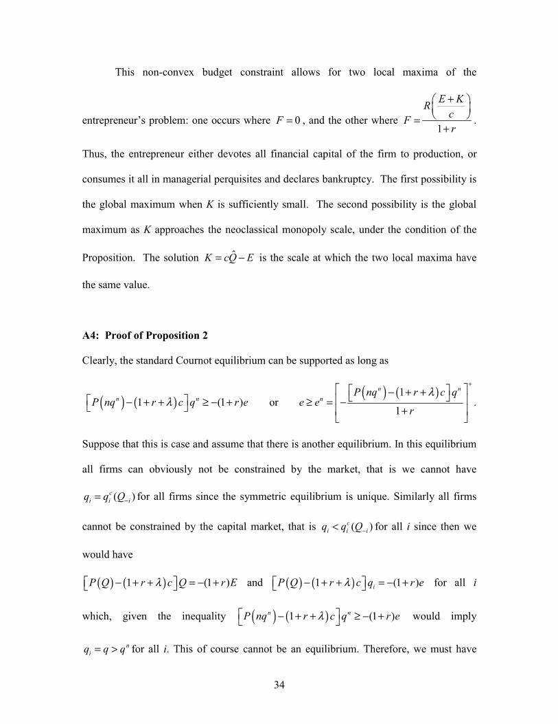
This non-convex budget constraint allows for two local maxima of the

entrepreneur’s problem: one occurs where 0F = , and the other where 1

E KRcFr

+ =

+.

Thus, the entrepreneur either devotes all financial capital of the firm to production, or

consumes it all in managerial perquisites and declares bankruptcy. The first possibility is

the global maximum when K is sufficiently small. The second possibility is the global

maximum as K approaches the neoclassical monopoly scale, under the condition of the

Proposition. The solution ˆK cQ E= − is the scale at which the two local maxima have

the same value.

A4: Proof of Proposition 2

Clearly, the standard Cournot equilibrium can be supported as long as

( ) ( )1 (1 )n nP nq r c q r eλ − + + ≥ − + or ( ) ( )1

1

n nn

P nq r c qe e

r

λ+

− + + ≥ = −+

.

Suppose that this is case and assume that there is another equilibrium. In this equilibrium

all firms can obviously not be constrained by the market, that is we cannot have

( )ci i iq q Q−= for all firms since the symmetric equilibrium is unique. Similarly all firms

cannot be constrained by the capital market, that is ( )ci i iq q Q−< for all i since then we

would have

( ) ( )1 (1 )P Q r c Q r Eλ− + + = − + and ( ) ( )1 (1 )iP Q r c q r eλ− + + = − + for all i

which, given the inequality ( ) ( )1 (1 )n nP nq r c q r eλ − + + ≥ − + would imply

niq q q= > for all i. This of course cannot be an equilibrium. Therefore, we must have

35

( )ni i iq q Q−< , ( )1iP q P r c′ + > + and ( ) ( )1 (1 )iP Q r c q r eλ− + + = − + for some i, and

( )nj j jq q Q−= , ( )1jP q P r c′ + = + and ( ) ( )1 (1 )jP Q r c q r eλ− + + ≥ − + for some j.

Comparing the incentive-compatibility expressions yields j iq q≤ while comparing the

Cournot first-order conditions yields j iq q> , an obvious contradiction.

Now assume that the unique and symmetric Cournot equilibrium cannot be supported by

the amount of inside equity., that is ( ) ( )1 (1 )n nP nq r c q r eλ − + + < − + . A similar

argument to the one above shows that we must have ˆniq q= for all i..

Finally note that if the total level of inside equity cannot support the unconstrained

equilibrium for n entrepreneurs, it cannot do so for (n+1) entrepreneurs either. To see

why, if the uncontrained equilibrium cannot be supported with n entrepreneurs, we have

( ) ( )1 (1 )n nP nq r c q r eλ − + + < − + and summing across firms

( ) ( )1 (1 )n nP Q r c Q r Eλ − + + < − + .

Therefore,

( ) ( ) ( ) ( )1 1 1 (1 )n n n n n nQ Q P Q r c Q P Q r c Q r Eλ λ+ ≥ ⇒ − + + ≤ − + + < − +

which implies that the unconstrained equilibrium cannot be supported with this level of

inside equity either.■

A5: Dynamics of Monopoly

We analyze how a longer horizon can relax the credit market incentive-

compatibility constraint that limits industry scale in a one-period market. We develop the

analysis for the case of a monopoly similar to the one before, except that the market

36

remains open for two periods. We demonstrate conditions under which the neoclassical

monopoly output obtains in the two-period model but not the one-period model, and

conversely.

Output is produced at two dates: { }1, 2t ∈ . In each period, demand is the same as

before. All inputs are variable, and must be purchased in advance of production in each

period. The production technology is constant returns as before and the interest rate is

constant over time.

We allow for long-term loan contracts, although these do not play a significant role in our

analysis. At the beginning of period t, the capital market advances tK , and, at the end of

the period, the firm repays ( )1 tr K+ . From an outside investor’s perspective a long term

loan contract is equivalent to a sequence of short-term contracts.13

The market unfolds as follows. At the beginning of period 1, the entrepreneur

invests financial capital 1E E= , as in the one-period model. The capital market supplies

additional funds 1K , and the firm produces 1 11

E KQc+= . At the beginning of period 2,

the entrepreneur has accumulated equity ( ) ( )2 1 11E R Q r K= − + , and produces

2 22

E KQc+= . The entrepreneur’s payoff at the end of the second period is

13 We assume that entrepreneur is free to arrange credit on any terms satisfying this condition and the additional incentive compatibility conditions introduced below. A standard long-term loan contract advances funds in stages. An outside investor lends 1

dollar in period 1 and another 2

1

Kk K= dollars in period 2. The firm repays ( )1 r+ at

the end of period 1 and another ( )1 r k+ at the end of period 2. This staged-finance contract is analogous to that analyzed by Bolton and Scharfstein (19xx), who make different assumptions about contractibility. Indeed, they consider the opposite case in which investment funds are contractible but sales revenues are not.

37

( ) ( )2 2 21R Q r Kπ = − + . There is no payoff at the end of the first-period, because profits

are fully reinvested assuming 2 0K > .

Capital market incentive-compatibility constraints assure outside investors that

the entrepreneur has no incentive to spend on managerial perquisites. The second-period

constraint is

2 2cQπ λ≥ .

The first-period constraint is

211 1

cQr r

π πλ≥ ++ +

,

where π is the second-period expected profit an entrepreneur who defaults in the first

period.

The value of π depends whether the entrepreneur’s monopoly property right is

protected in bankruptcy. We assume so.14 More precisely we assume that an

entrepreneur who defaults cannot be prevented from starting a new firm but that funds

that are converted into private benefits cannot be used as equity. Let 0Q̂ be the strictly

positive root of 0 0ˆ ˆ( ) (1 ) 0R Q r cQλ− + + = , and assume 0

ˆMQ Q< . Then an entrepreneur

with zero equity at the beginning of the second-period produces 0Q̂ with borrowed funds,

and earns an end-of-period profit 0ˆcQπ λ= . Therefore, the first-period incentive

compatibility constraint is

021

ˆ

1 1Qc Q

r rπ λ

≥ + + +

.

14 The exact solution of the dynamic game obviously depends upon the entrepreneur’s outside option; however, the qualitative insights are robust.

38

Suppose that the two incentive compatibility constraints are slack. It is

straightforward to prove that optimal credit market arrangements allow the neoclassical

monopoly output MQ in both periods. At the neoclassical solution, the entrepreneur

earns

( ) ( ) ( ) ( )22 1 2 1M Mr E r R Q r cQπ = + + + − + .

All of the entrepreneur’s return comes at the end of the second period, and consists of a

normal return on inside equity plus compounded monopoly rents. At the neoclassical

solution, the first-period incentive constraint implies the second-period constraint.

Therefore, both constraints are indeed satisfied if

( )

( ) ( )02

ˆ 2 11 1 1

M M MQc rE Q P Q r c Qr r r

λ + ≥ + − − + + + + .

How does this industry outcome contrast with the one period model? In the one

period model, an entrepreneur with equity E is constrained by the credit market if

ˆ MQ Q< . This condition is equivalent to

( ) ( )1

1

M MP Q r c QE

r

λ − + + < −+

.

Therefore, we have the following result.

Proposition 4 If

( )( ) ( )

( ) ( )0

2

ˆ 12 11 1 11

M MM M M

P Q r c QQc rQ P Q r c Q Er r rr

λλ − + + + + − − + ≤ < − + + ++

then 1 2MQ Q Q= = in the two-period model, while MQ Q< in the one-

period model .

39

Thus there exist a range of circumstances when the capital market constrains

industry scale in the one-period monopoly model, but not in the two-period model. The

conditions defining these circumstances are nondegenerate if

( )

( ) ( )( ) ( )

02

ˆ 12 11 1 11

M MM M M

P Q r c QQc rQ P Q r c Qr r rr

λλ − + + + + − − + < − + + ++ .

A few simple algebraic manipulations reduce this inequality to

( ) ( ) 0ˆ1M MR Q r cQ cQλ− + > ,

which must hold given the definition of 0Q̂ and MQ (i.e. the very definition of these

variables yields ( ) ( ) ( ) ( )0 0 0ˆ ˆ ˆ1 1M MR Q r cQ R Q r cQ cQλ− + > − + = ).

A6: Proof of Proposition 3

Define ˆ( , )iq Q e and ( )q Q respectively by the equations

( ) ( ) ˆ1 ( , ) (1 )i iP Q r c q Q e r eλ− + + = − + and ( ) ( ) ( )( ) 1P Q q Q P Q r c′ + = + . If Q is the

total equilibrium output, then each firm’s output is described by

{ }ˆ( ) min ( , ), ( )i iq Q q Q e q Q= . It is easy to verify that both ˆ( , )iq Q e and ( )q Q are

decreasing functions of Q. As a consequence ( )iq Q is also decreasing in Q and the fixed

point ( )ii

Q q Q=∑ is unique which implies that any equilibrium is also unique.

Suppose that firm i is constrained then ( ) ( )(1 ) 1i iP Q r c q r eλ− + + = − + and

( )ni i iq q Q−< . The last inequality implies ( ) ( ) ( )1iP Q q P Q r c′ + > + . If firm j is not

40

constrained then ( ) ( )(1 ) 1j jP Q r c q r eλ− + + ≥ − + and ( )nj j jq q Q−= which implies

( ) ( ) ( )1jP Q q P Q r c′ + = + . Given the model’s assumptions, and the fact that in

equilibrium all funds are used for production:

a) the first order conditions above clearly imply i jq q< and i i j je k e k+ < + ;

b) the two incentive compatibility constraints imply

( )(1 )(1 )

i

i i

P r c er c e k

λ− + +− =

+ + ( )(1 )

(1 )j

j j

eP r cr c e k

λ− + +− ≤

+ +

which clearly implies ji

i i j j

eee k e k

≤+ +

. This inequality implies that if i je e> then i jk k> .

Since we have i i j je k e k+ < + we can therefore not have i je e> . Therefore unconstrained

firms have more equity than constrained firms.

If firms i and j are both constrained it is straightforward that ji

i i j j

eee k e k

=+ +

and that

i j i j i je e k k q q< ⇒ < ⇒ < . Finally it is obvious that when a constrained firm i is split

into m smaller firms 1

m

i ijj

e e=

=∑ , in the new equilibrium the output of the original firm is

simply split among the new firms proportionally to equity ijij i

i

eq q

e= since

( ) ( )(1 ) 1ij ijP Q r c q r eλ− + + = − + and ( ) ( ) ( )1ijP Q q P Q r c′ + > + ■

41

REFERENCES Albuquerque, Rui and Hugo A. Hopenhayn, 2002, “Optimal Lending Contracts and Firm Dynamics,” Review of Economic Studies, forthcoming. Allen, Franklin and Douglas Gale, 2000, “Corporate governance and competition”, Corporate governance: theoretical and empirical perspectives, Xavier Vives ed., Cambridge University Press, 23-84. Amir, Rabah, and Val E. Lambson, 2000,”On the effects of entry in Cournot markets”, Review of Economic Studies, 67, 235-254. Brander, James and Tracy Lewis, 1986, “Oligopoly and Financial Structure: The Limited Liability Effect", American Economic Review, 76, 956-970. Bolton, Patrick and David Scharfstein, 1990, “A Theory of Predation Based on Agency Problems in Financial Contracting", American Economic Review, 80, 93-106. Brander, James and Tracy Lewis, 1986, “Oligopoly and Financial Structure: The Limited Liability Effect", American Economic Review, 76, 956-970. Busse, Meghan R., 2002, “Firm Financial Condition and Airline Price Wars,” RAND Journal of Economics, 33, 298-318. Chevalier, Judith A., 1995a, “Capital Structure and Product-Market Competition: Empirical Evidence from the Supermarket Industry,” American Economic Review, 85, 415-35. Chevalier, Judith A. 1995b, “Do LBO Supermarkets Charge More? An Empirical Analysis of the Effects of LBOs on Supermarket Pricing,” Journal of Finance, 50, 1095-112. Chevalier, Judith A. and David S. Scharfstein, 1995, “Liquidity Constraints and the Cyclical Behavior of Markups”, American Economic Review, 85(2), 390-96. Chevalier, Judith A. and David S. Scharfstein, 1996, “Capital-Market Imperfections and Countercyclical Markups: Theory and Evidence”, American Economic Review, 86(4), 703-25. Hart, Oliver D., 1983, “The market mechanism as an incentive device”, The Bell Journal of Economics, 14, 366-382. Hermalin, Benjamin E., 1992, “The effect of competition on executive behavior”, RAND Journal of Economics, 23(3), 350-365.

42

Jensen, Michael C., and William H. Meckling, 1976, “Theory of the Firm: Managerial Behavior, Agency Costs and Ownership Structure”, Journal of Financial Economics, 3(4), 305-60. Kovenock, Dan and Gordon M. Phillips, 1997, “Capital Structure and Product Market Behavior: An Examination of Plant Exit and Investment Decisions”, Review of Financial Studies, 10(3), 767-803. Kreps, David M. and Jose A. Scheinkman, 1983, “Quantity Precommitment and Bertrand Competition Yield Cournot Outcomes”, Bell Journal of Economics, 14(2), 326-37. Maksimovic, Vojislav, 1988, “Capital Structure in Repeated Oligopolies”, RAND Journal of Economics, 19, 389-407. Modigliani, Franco and Merton Miller, 1958, “The Cost of Capital, Corporate Finance, and the Theory of Investment”, American Economic Review, 48, 261-97 Phillips, Gordon M., 1995, “Increased Debt and Industry Product Markets: An Empirical Analysis”, Journal of Financial Economics, 37(2), 189-238. Raith, Michael, 2002, “Competition, Risk and Managerial Incentives", forthcoming in American Economic Review. Salant, Stephen, Sheldon Switzer, and Robert J. Reynolds, 1983, “Losses from horizontal merger: the effects of an exogenous change in industry structure on Cournot-Nash equilibrium”, Quarterly Journal of Economics, 98(2), 185-199. Scharfstein, David, 1988, “Product-market competition and managerial slack”, RAND Journal of Economics, 19(1), 147-155. Schmidt, Klaus M., 1997, “Managerial incentives and product market competition”, Review of Economic Studies, 64, 191-213. Showalter, Dean M., 1995, “Oligopoly and Financial Structure: Comment”, American Economic Review, 85, 647-653.

Showalter, Dean M., 1999, “Debt as an Entry Deterrent under Bertrand Price Competition”, Canadian Journal of Economics, 32, 1069-81. Townsend, Robert M, 1979,”Optimal contracts and competitive markets with costly state verification”, Journal of Economic Theory, 21(2), 265-293. Williams, Joseph T, 1995, “Financial and Industrial Structure with Agency”, Review of Financial Studies, 8(2), 431-74.

λcQ-(1+r)E

W(Q)

MQ

Output is constrain .

Q̂

Figure 1: ed below the monopoly level

43

44

( )Ciq Q−

ˆ( )iq Q−1iQ

n−

−

ˆnq

nq

MQ

iQ−

iq

Figure 2: Capital market constrains best response curve.

45

Perks

Output Manager’sUtility

Manager’sUtility

Output

Perks

(a)

(b)

Figure 3: The entrepreneur’s choice between production and perquisites:

(a) Jensen and Meckling (1976) (b) The unconstrained entrepreneur

46

Manager’sUtility

Output

Perks

Figure 3 (c) The entrepreneur’s choice between production and perquisites:

The constrained entrepreneur