Capital Deepening and Non-Balanced Economic Growth∗

Daron AcemogluMIT

Veronica GuerrieriMIT

First Version: May 2004.This Version: June 2005.

Still Preliminary. Comments Welcome.

Abstract

This paper constructs a model of non-balanced economic growth. The main economicforce is the combination of differences in factor proportions and capital deepening. Capitaldeepening tends to increase the relative output of the sector with a greater capital share(despite the equilibrium reallocation of capital and labor away from that sector). We firstillustrate this force using a general two-sector model. We then investigate it further usinga class of models with constant elasticity of substitution between two sectors and Cobb-Douglas production functions in each sector. In this class of models, non-balanced growthis shown to be consistent with an asymptotic equilibrium with constant interest rate andcapital share in national income. Finally, we construct and analyze a model of “non-balanced endogenous growth,” which extends these results to an economy with endogenousand directed technical change, and demonstrates that non-balanced technological progresscan be an equilibrium phenomenon.

Keywords: capital deepening, endogenous growth, multi-sector growth, non-balancedeconomic growth.JEL Classification: O40, O41, O30.

∗We thank seminar participants at Chicago, Federal Reserve Bank of Richmond, MIT, Society of EconomicDynamics, Florence 2004, and Universitat of Pompeu Fabra for useful comments and Ariel Burstein for helpwith the simulations. Acemoglu acknowledges financial support from the Russell Sage Foundation and the NSF.An early version of this paper was circulated under the title “Non-Balanced Endogenous Growth”.

1

1 Introduction

Most models of economic growth strive to be consistent with the Kaldor facts, i.e., the relative

constancy of the growth rate, the capital-output ratio, the share of capital income in GDP

and the real interest rate (see Kaldor, 1963, and also Denison, 1974, Barro and Sala-i-Martin,

2004). Beneath this balanced picture, however, are the patterns that Kongsamut, Rebelo

and Xie (2001) refer to as the Kuznets facts, which concern the systematic change in the

relative importance of various sectors, in particular, agriculture, manufacturing and services

(see Kuznets, 1957, 1973, Chenery, 1960, Kongsamut, Rebelo and Xie, 2001). While the

Kaldor facts emphasize the balanced nature of economic growth, the Kuznets facts highlight

its non-balanced nature.

The Kuznets facts have motivated a small literature, which typically starts by positing non-

homothetic preferences consistent with Engel’s law. With these preferences, the marginal rate

of substitution in consumption changes as an economy grows, directly leading to a pattern

of non-balanced growth (e.g., Murphy, Shleifer and Vishny, 1989, Matsuyama, 1992, 2005,

Echevarria, 1997, Laitner, 2000, Kongsamut, Rebelo and Xie, 2001, Caselli and Coleman, 2001,

Gollin, Parente and Rogerson, 2002). An alternative perspective, proposed by Baumol (1967),

emphasizes the potential non-balanced nature of economic growth resulting from differential

productivity growth across sectors, but has received less attention in the literature.1

This paper has two aims. First, it shows that there is another, and very natural, reason to

expect economic growth to be non-balanced. Differences in factor proportions across sectors

(i.e., different shares of capital) combined with capital deepening will lead to non-balanced

growth. The reason is simple: an increase in capital-labor ratio will raise output more in

the sector with greater capital intensity. More specifically, we prove that with balanced tech-

nological progress (in the sense of equal rates of Hicks-neutral technological progress across

sectors), capital deepening and differences in factor proportions necessarily cause non-balanced

growth. This result holds irrespective of the exact source of economic growth or the process of

accumulation.

The second objective of the paper is to present and analyze a tractable two-sector growth

1An exception is the recent independent paper by Ngai and Pissarides (2005), which constructs a modelof multi-sector economic growth inspired by Baumol. In Ngai and Pissarides’s model, there are exogenousTFP differences across sectors, but all sectors have identical Cobb-Douglas production functions. Consequently,although their model is potentially consistent with the Kuznets and Kaldor facts, it does not contain themain contribution of our paper, non-balanced growth resulting from factor proportion differences and capitaldeepening.

1

model featuring non-balance growth. We do this by constructing a class of economies with

constant elasticity of substitution between two sectors and Cobb-Douglas production functions

within each sector. We investigate the equilibrium of such an economy with exogenous and

endogenous technological change. We show that equilibrium takes a simple form, with constant

growth rate in all sectors, constant interest rate and constant share of capital in national income

in the limiting (asymptotic) equilibrium.

The form of the limiting equilibrium of this class of economies depends on whether the

products of the two sectors are gross substitutes or complements (meaning whether the elas-

ticity of substitution between these products is greater than or less than one). When they are

gross substitutes, the sector that is more “capital intensive” (in the sense of having a greater

capital share) dominates the economy. The form of the equilibrium is more interesting when

the elasticity of substitution between these products is less than one. In this case, the growth

rate of the economy is determined by the more slowly growing (less capital-intensive sector).

Despite the change in the terms of trade against the faster growing sector, in equilibrium suf-

ficient amounts of capital and labor (and technological progress when this is endogenous) are

deployed in this sector to ensure a faster rate of growth.

One interesting feature is that, especially when the elasticity of substitution is less than

one,2 the resulting pattern of economic growth is consistent with the Kuznets facts, without

substantially deviating from the Kaldor facts. In particular, even in the limiting equilibrium

both sectors grow with positive (and unequal) rates, and more importantly, we show that

convergence to this limiting equilibrium may be slow, and along the transition path, growth

is non-balanced, while capital share and interest rate vary only by relatively small amounts.

Therefore, the equilibrium with an elasticity of substitution less than one may be able to

rationalize both the Kuznets and the Kaldor facts. Naturally, whether or not this is the

2As we will see below, the elasticity of substitution between products will be less than one if and only if the(short-run) elasticity of substitution between labor and capital is less than one. In view of the time-series andcross-industry evidence, a short-run elasticity of substitution between labor and capital less than one appearsreasonable.For example, Hamermesh (1993), Nadiri (1970) and Nerlove (1967) survey a range of early estimates of the

elasticity of substitution, which are generally between 0.3 and 0.7. David and Van de Klundert (1965) similarlyestimate this elasticity to be in the neighborhood of 0.3. Using the translog production function, Griffin andGregory (1976) estimate elasticities of substitution for nine OECD economies between 0.06 and 0.52. Berndt(1976), on the other hand, estimates an elasticity of substitution equal to 1, but does not control for a timetrend, creating a strong bias towards 1. Using more recent data, and various different specifications, Krusell,Ohanian, Rios-Rull, and Violante (2000) and Antras (2001) also find estimates of the elasticity significantlyless than 1. Estimates implied by the response of investment to the user cost of capital also typically imply anelasticity of substitution between capital and labor significantly less than 1 (see, e.g., Chirinko, 1993, Chirinko,Fazzari and Mayer, 1999, or Mairesse, Hall and Mulkay, 1999).

2

empirically correct explanation is not answered by this theoretical result.

Finally, we present and analyze a model of “non-balanced endogenous growth,” which shows

the robustness of our results to endogenous technological progress, and demonstrates how, in

the presence of factor proportion differences, the pattern of technological progress itself will

be non-balanced. To the best of our knowledge, despite the large literature on endogenous

growth, there are no previous studies that combine endogenous technological progress and

non-balanced growth.3

The rest of the paper is organized as follows. Section 2 shows how the combination of factor

proportions differences and capital deepening lead to non-balanced growth using a general

two-sector growth model. Section 3 constructs a more specific model with a constant elasticity

of substitution between two sectors and Cobb-Douglas production functions, but exogenous

technological progress. It characterizes the full dynamic equilibrium of this economy, and shows

how with an elasticity of substitution less than one, the model may generate an equilibrium

path that is consistent both with the Kuznets and the Kaldor facts. Section 4 introduces

endogenous technological progress and shows that the results are robust to differential rates of

technological progress across sectors. Section 5 concludes, and the Appendix contains proofs

that are not presented in the text.

2 Capital Deepening and Non-Balanced Growth

We first illustrate how differences in factor proportions across sectors combined with capital

deepening lead to non-balanced economic growth. To do this, we use a standard two-sector

competitive model with constant returns to scale in both sectors, and two factors of production,

capital, K, and labor, L. To highlight that the exact nature of the accumulation process is

not essential for the results, in this section we take the sequence (process) of capital and

labor supplies, [K (t) , L (t)]∞t=0, as given (and assume that labor is supplied inelastically). In

addition, we omit explicit time dependence when this will cause no confusion.

Final output, Y , is produced as an aggregate of the output of two sectors, Y1 and Y2,

Y = F (Y1, Y2) ,

3See, among others, Romer (1986, 1990), Lucas (1988), Rebelo (1991), Segerstrom, Anant and Dinopoulos(1990), Grossman and Helpman (1991a,b), Aghion and Howitt (1992), Jones (1995), Young (1993). Aghionand Howitt (1998) and Barro and Sala-i-Martin (2004) provide excellent introductions to endogenous growththeory. See also Acemoglu (2002) on models of directed technical change that feature endogenous, but balancedtechnological progress in different sectors. Acemoglu (2003) presents a model with non-balanced technologicalprogress between two sectors, but in the limiting equilibrium both sectors grow at the same rate.

3

and we assume that F exhibits constant returns to scale and is continuously differentiable.

Output in both sectors is produced with the production functions

Y1 = A1G1 (K1, L1) (1)

and

Y2 = A2G2 (K2, L2) . (2)

G1 and G2 also exhibit constant returns to scale and are twice differentiable. A1 and A2

denote Hicks-neutral technology terms.4 We also assume that the functions F , G1 and G2

satisfy Inada-type conditions, e.g., limY1→0 ∂F (Y1, Y2) /∂Y1 = ∞ for all Y2 > 0, etc. These

assumptions ensure interior solutions and simplify the exposition, though they are not necessary

for the results presented in this section.

Market clearing implies

K1 +K2 = K, (3)

L1 + L2 = L,

where K and L are the (potentially time-varying) supplies of capital and labor, given by the

exogenous sequence [K (t) , L (t)]∞t=0, which we take to be continuosly differentiable functions

of time. Without loss of any generality, we also ignore capital depreciation.

We normalize the price of the final good to 1 in every period, and denote the prices of Y1

and Y2 by p1 and p2, and wage and rental rate of capital (interest rate) by w and r. We assume

that product and factor markets are competitive, so product prices satisfy

p1p2=

∂F (Y1, Y2) /∂Y1∂F (Y1, Y2) /∂Y2

, (4)

and the wage and the interest rate satisfy5

w =∂A1G1 (K1, L1)

∂L1=

∂A2G2 (K2, L2)

∂L2(5)

r =∂A1G1 (K1, L1)

∂K1=

∂A2G2 (K2, L2)

∂K2.

4Allowing more general forms of technological progress would complicate the analysis since we would haveto rule out a change in the marginal rates of substitution between capital and labor in G1 and G2 with changesin A1 and A2 that would “by chance” satisfy the conditions necessary for balanced growth.

5Without the Inada-type assumptions, these would have to be written as

w ≥ ∂A1G1 (K1, L1) /∂L1 and L1 ≥ 0,

with complementary slackness, etc.

4

An equilibrium, given factor supply sequences, [K (t) , L (t)]∞t=0, is a sequence of product

and factor prices, [p1 (t) , p2 (t) , w (t) , r (t)]∞t=0 and factor allocations,

[K1 (t) ,K2 (t) , L1 (t) , L2 (t)]∞t=0, such that (3), (4) and (5) are satisfied.

Also define the share of capital in the two sectors

s1 ≡rK1

p1Y1and s2 ≡

rK2

p2Y2,

the capital to labor ratio in the two sectors,

k1 ≡K1

L1and k2 ≡

K2

L2

and the “per capita production functions” (without the Hicks-neutral technology term),

g1 (k1) ≡G1 (K1, L1)

L1and g2 (k2) ≡

G2 (K2, L2)

L2.

We say that there is capital deepening in the economy if K/K > L/L and there is factor

proportion differences if s1 6= s2.6 The next theorem shows that if there is capital deepening

and factor proportion differences, then balanced technological progress is not consistent with

balanced growth.

Theorem 1 Suppose that at time t, there are factor proportion differences between the two

sectors, i.e., s1 (t) 6= s2 (t), technological progress is balanced, i.e., A1 (t) /A1 (t) = A2 (t) /A2 (t)

and there is capital deepening, i.e., K (t) /K (t) > L (t) /L (t), then growth is not balanced,

that is, Y1 (t) /Y1 (t) 6= Y2 (t) /Y2 (t).

Proof. Differentiating the production function for the two sectors,

Y1Y1=

A1A1

+ s1K1

K1+ (1− s1)

L1L1

andY2Y2=

A2A2

+ s2K2

K2+ (1− s2)

L2L2

.

Suppose, to obtain a contradiction, that Y1/Y1 = Y2/Y2. Since A1/A1 = A2/A2 and s1 6= s2,

this implies k1/k1 6= k2/k2 (otherwise, k1/k1 = k2/k2 > 0 because of capital deepening and if,

for example, s1 < s2, then Y1/Y1 < Y2/Y2).

6Here s1 (t) 6= s2 (t) refers to the equilibrium factor proportions in the two sectors at time t. It does notnecessarily mean that these will not be equal at some future date.

5

Since F exhibits constant returns to scale, (4) implies

p1p1=

p2p2= 0. (6)

Equation (5) yields the following interest rate and wage conditions

r = p1A1g01 (k1) (7)

= p2A2g02 (k2) ,

and

w = p1A1¡g1 (k1)− g01 (k1) k1

¢(8)

= p2A2¡g2 (k2)− g02 (k2) k2

¢.

Differentiating the interest rate condition, (7), with respect to time and using (6), we have

A1A1

+ εg01k1k1=

A2A2

+ εg02k2k2

where

εg01 ≡g001 (k1) k1g01 (k1)

and εg02 ≡g002 (k2) k2g02 (k2)

.

Since A1/A1 = A2/A2, we must have

εg01k1k1= εg02

k2k2. (9)

Differentiating the wage condition, (8), with respect to time, using (6) and some algebra

givesA1A1− s11− s1

εg01k1k1=

A2A2− s21− s2

εg02k2k2.

Since A1/A1 = A2/A2 and s1 6= s2, this equation is inconsistent with (9), yielding a contradic-

tion and proving the claim.

The intuition for this result can be obtained as follows. Suppose there is capital deepening

and that both capital and labor are allocated to the two sectors with constant proportions.

Because factor proportions differ between the two sectors, say s1 < s2, such an allocation will

generate faster growth in sector 2 than in sector 1 and induce a non-balanced pattern of growth

(since there is capital deepening). In equilibrium, the faster growth in sector 2 will naturally

change equilibrium prices, and the decline in the relative price of sector 2 will cause some of

6

the labor and capital to be reallocated to sector 1. However, this reallocation cannot entirely

offset the greater increase in the output of sector 2, since, if it did, the relative price change

that stimulated the reallocation would not take place. Consequently, equilibrium growth will

be non-balanced.

The proof of Theorem 1 makes it clear that the two-sector structure is not necessary for

this result. In light of this, we also state a generalization for N ≥ 2 sectors, where aggregateoutput is given by the constant returns to scale production function

Y = F (Y1, Y2, ..., YN) .

The definitions for s, k and g and the other assumptions above naturally generalize to this

setting. We have:

Theorem 2 Suppose that at time t, there are factor proportion differences among the N

sectors in the sense that there exists i and j ≤ N such that si (t) 6= sj (t), technological

progress is balanced, i.e., Ai (t) /Ai (t) = Aj (t) /Aj (t) for all i and j ≤ N , and there is capital

deepening, i.e., K (t) /K (t) > L (t) /L (t), then growth is not balanced, that is, there exists i

and j ≤ N such that Yi (t) /Yi (t) 6= Yj (t) /Yj (t).

The proof of this theorem parallels that of Theorem 1 and is omitted.

3 Two-Sector Growth with Exogenous Technology

The previous section demonstrated that differences in factor proportions across sectors and

capital deepening will lead to non-balanced growth. This result was proved for a given (ar-

bitrary) sequence of capital and labor supplies, [K (t) , L (t)]∞t=0, but this level of generality

does not allow us to fully characterize the equilibrium path and its limiting properties. We

now wish to analyze the equilibrium behavior of such an economy fully, which necessitates at

least the sequence of capital stocks to be endogenized, and capital deepening to emerge as an

equilibrium phenomenon. We will accomplish this by imposing more structure both in terms of

specifying preferences and in terms of the production functions. Capital deepening will result

from exogenous technological progress, which will in turn be endogenized in Section 4.

7

3.1 Demographics, Preferences and Technology

The economy consists of L (t) workers at time t, supplying their labor inelastically. There is

exponential population growth,

L (t) = exp (nt)L (0) . (10)

We assume that all households have constant relative risk aversion (CRRA) preferences over

total household consumption (rather than per capita consumption), and all population growth

takes place within existing households (thus there is no growth in the number of households).7

This implies that the economy admits a representative agent with CRRA preferences (see, for

example, Caselli and Ventura, 2000):Z ∞

0

C(t)1−θ − 11− θ

e−ρtdt,

where C (t) is aggregate consumption at time t, ρ is the rate of time preferences and θ ≥ 0is the inverse of the intertemporal elasticity of substitution (or the coefficient of relative risk

aversion). We again drop time arguments to simplify the notation whenever this causes no

confusion, and continue to assume that there is no depreciation of capital. The flow budget

constraint for the representative consumer is:

K = rK + wL+Π−C, (11)

where K and L denote the total capital stock and the total labor force in the economy, Π is

total net corporate profits received by the consumers, w is the equilibrium wage rate and r is

the equilibrium interest rate.

The unique final good is produced by combining the output of two sectors with elasticity

of substitution ε ∈ [0,∞):

Y =

∙γY

ε−1ε

1 + (1− γ)Yε−1ε

2

¸ εε−1

, (12)

where γ is a distribution parameter which determines the relative importance of the two goods

in the aggregate production.

The resource constraint of the economy, in turn, requires that consumption and investment

are less than total output, Y = rK + wL+Π, thus

K + C ≤ Y. (13)7The alternative would be to specify population growth taking place at the extensive margin, in which case

the discount rate of the representative agent would be ρ− n rather than ρ, without any substantive changes inthe analysis.

8

The two goods Y1 and Y2 are produced competitively using constant elasticity of substitu-

tion (CES) production functions with elasticity of substitution between intermediates equal to

ν > 1:

Y1 =

µZ M1

0y1(i)

ν−1ν di

¶ νν−1

and Y2 =

µZ M2

0y2(i)

ν−1ν di

¶ νν−1

, (14)

where y1(i)’s and y2(i)’s denote the intermediates in the sectors that have different capi-

tal/labor ratios, andM1 andM2 represent the technology terms. In particularM1 denotes the

number of intermediates in sector 1 and M2 the number of intermediate goods in sector 2.

Intermediate goods are supplied by monopolists that hold the relevant patent,8 and are

produced with the following Cobb-Douglas technologies

y1(i) = l1(i)α1k1(i)

1−α1 and y2 (i) = l2 (i)α2 k2 (i)

1−α2 , (15)

where l1(i) and k1(i) are labor and capital used in the production of good i of sector 1 and

l2 (i) and k2 (i) are labor and capital used in the production of good i of sector 2.9

The parameters α1 and α2 determine which sector is more “capital intensive”.10 When

α1 > α2, sector 1 is less capital intensive, while the converse applies when α1 < α2. In the rest

of the analysis, we assume that

α1 > α2, (A1)

which only rules out the case where α1 = α2, since the two sectors are otherwise identical and

the labeling the sector with the greater capital share is without loss of any generality.

All factor markets are competitive, and market clearing for the two factors implyZ M1

0l1(i)di+

Z M2

0l2 (i) di ≡ L1 + L2 = L, (16)

and Z M1

0k1(i)di+

Z M2

0k2 (i) di ≡ K1 +K2 = K, (17)

8Monopoly power over intermediates is introduced to create continuity with the next section, where monopolyprofits will motivate the creation of new intermediates. Since equilibrium markups will be constant, thismonopoly power does not have any substantive effect on the form of equilibrium.

9Strictly speaking, we should have two indices, i1 ∈ [0,M1] and i2 ∈ [0,M2], but we simplify the notation byusing a generic i to denote both indices, and let the context determine which index is being referred to.10We use the term “capital intensive” as corresponding to a greater share of capital in value added, i.e.,

meaning for example that s1 > s2 in terms of the notation of the previous section. While this share is constantbecause of the Cobb-Douglas technologies, the equilibrium ratios of capital to labor in the two sectors dependon prices.

9

where the first set of equalities in these equations define K1, L1 and K2, L2 as the levels of

capital and labor used in the two sectors, and the second set of equalities impose market

clearing.

The number of intermediate goods in the two sectors evolve at the exogenous rates

M1

M1= m1 and

M2

M2= m2, (18)

and each new intermediate is assigned to a monopolist, so that all intermediate goods are

owned and produced by monopolists throughout. Since M1 and M2 determine productivity in

their respective sectors, we will refer to them as “technology”.

3.2 Equilibrium

Recall that w and r denote the wage and the capital rental rate, and p1 and p2 denote the

prices of the Y1 and Y2 goods, with the price of the final good normalized to one. Let [q1(i)]M1i=1

and [q2(i)]M2i=1 be the prices for labor-intensive and capital-intensive intermediates.

An equilibrium in this economy is given by paths for factor, intermediate and final goods

prices r, w, [q1(i)]M1i=1 , [q2(i)]

M2i=1 , p1 and p2, employment and capital allocation [l1(i)]

M1i=1 ,

[l2(i)]M2i=1 , [k1(i)]

M1i=1 , [k2(i)]

M2i=1 such that firms maximize profits and markets clear, and con-

sumption and savings decisions, C and K, maximize consumer utility.

It is useful to break the characterization of equilibrium into two pieces: static and dynamic.

The static part takes the state variables of the economy, which are the capital stock, the labor

supply and the technology, K, L,M1 andM2, as given, and determines the allocation of capital

and labor across sectors and factor and good prices. The dynamic part of the equilibrium

determines the evolution of the endogenous state variable, K (the dynamic behavior of L is

given by (10) and the one of M1 and M2 by (18)).

First, our choice of numeraire implies that the price of the final good, P , satisfies:

1 ≡ P =£γεp1−ε1 + (1− γ)ε p1−ε2

¤ 11−ε .

Next, since Y1 and Y2 are supplied competitively, their prices are equal to the value of their

marginal product, thus

p1 = γ

µY1Y

¶−1ε

and p2 = (1− γ)

µY2Y

¶− 1ε

, (19)

10

and the demands for intermediates, y1(i) and y2(i), are given by the familiar isoelastic demand

curves:q1(i)

p1=

µy1(i)

Y1

¶− 1ν

andq2(i)

p2=

µy2(i)

Y2

¶− 1ν

. (20)

The value of the monopolist for intermediate i in the s-intensive sector is given by

Vs(i, t) =

Z ∞

texp

∙−Z v

tr(z)dz

¸πs(i, v)dv, (21)

for s = 1, 2, where πs (i, t) = (qs (i, t)−mcs (i, t)) ys (i, t) is the flow profits for firm i at time

t, with qs given by the demand curves in (20), and mcs is the marginal cost of production in

this sector. Given the production functions in (15), the cost functions take the familiar Cobb-

Douglas form,mc1 (i) = α−α11 (1− α1)α1−1 r1−α1wα1 , andmc2 (i) = α−α22 (1− α2)

α2−1 r1−α2wα2 .

In equilibrium, all firms in the same sector will make the same profits, so we have Vs(i, t) =

Vs(t), and we use V1(t) and V2(t) to denote the value firms in the two sectors at time t. In

Section 4, these value functions will be used to determine the equilibrium growth rate of the

number of intermediate goods, M1 and M2.

Each monopolist chooses its price to maximize (21). Since prices at time t only influence

revenues and costs at that point, profit-maximizing prices will be given by a constant mark-up

over marginal cost:

q1(i) =

µν

ν − 1

¶α1 (1− α1)

α1−1 r1−α1wα1 , (22)

q2(i) =

µν

ν − 1

¶α2 (1− α2)

α2−1 r1−α2wα2 . (23)

Equations (22) and (23) imply that all intermediates in each sector sell at the same price

q1 = q1(i) for all i ≤ M1 and q2 = q2(i) for all i ≤ M2. This combined with (20) implies that

the demand for, and the production of, the same type of intermediate will be the same. Thus:

y1(i) = l1 (i)α1 k1 (i)

1−α1 = y1 = lα11 k1−α11 ∀i ≤M1

y2(i) = l2 (i)α2 k2 (i)

1−α2 = y2 = lα22 k1−α22 ∀i ≤M2,

where l1 is the level of employment in all intermediates of sector 1, etc.

Market clearing conditions, (16) and (17), then imply that l1 = L1/M1, k1 = K1/M1,

l2 = L2/M2 and k2 = K2/M2, so we have the output of each intermediate in the two sectors as

y1 =Lα11 K1−α1

1

M1and y2 =

Lα22 K1−α2

2

M2. (24)

11

Substituting (24) into (14), we obtain the total supply of labor- and capital-intensive goods

as

Y1 =M1

ν−11 Lα1

1 K1−α11 and Y2 =M

1ν−12 Lα2

2 K1−α22 . (25)

Comparing these (derived) production functions to (1) and (2) highlights that in this economy,

the production functions G1 and G2 from the previous section take Cobb-Douglas forms,

with one sector always having a higher share of capital than the other sector, and also that

A1 =M1

ν−11 and A2 =M

1ν−12 .

In addition, combining (25) with (12) implies that the aggregate output of the economy is:

Y =

"γ

µM

1ν−11 Lα1

1 K1−α11

¶ ε−1ε

+ (1− γ)

µM

1ν−12 Lα2

2 K1−α22

¶ ε−1ε

# εε−1

. (26)

Using (24) and (25) we can rewrite the prices for the labor- and capital-intensive interme-

diates as q1 = γM1

ν−11

¡Y1Y

¢− 1ε and q2 = (1− γ)M

1ν−12

¡Y2Y

¢− 1ε , and the flow profits from the

sale of the labor- and capital-intensive intermediates are:

π1 =γ

ν

µY1Y

¶−1ε Y1

M1and π2 =

1− γ

ν

µY2Y

¶− 1ε Y2M2

. (27)

Finally, factor prices and the allocation of capital between the two sectors are determined

by:11

w =

µν − 1ν

¶γα1

µY

Y1

¶ 1ε Y1L1

(28)

w =

µν − 1ν

¶(1− γ)α2

µY

Y2

¶ 1ε Y2L2

(29)

r =

µν − 1ν

¶γ (1− α1)

µY

Y1

¶ 1ε Y1K1

(30)

r =

µν − 1ν

¶(1− γ) (1− α2)

µY

Y2

¶ 1ε Y2K2

. (31)

These factor prices take the familiar form, equal to the marginal product of a factor from (26)

with a discount, (ν − 1) /ν, due to the the monopoly markup in the intermediate goods.11To obtain these equations, start with the cost functions above, and derive the demand for factors by using

Shepherd’s Lemma. For example, for the sector 1, these are l1 =³

α11−α1

rw

´1−α1y1 and k1 =

³α1

1−α1rw

´−α1y1.

Combine these two equations to derive the equilibrium relationship between r and w. Then using equation (22),eliminate r to obtain a relationship between w and q1. Now combining with the demand curves in (20), themarket clearing conditions, (16) and (17), and using (25) yields (28). The other equations are obtained similarly.

12

3.3 Static Equilibrium: Comparative Statics

Let us now analyze how changes in the state variables, L,K,M1 andM2, impact on equilibrium

factor prices and factor shares. As noted in the Introduction, the case with ε < 1 is of greater

interest (and empirically more relevant as pointed out in footnote 2), so throughout, we focus

on this case (though we give the result for the case in which ε > 1, and we only omit the case

with ε = 1, which is standard).

Let us denote the fraction of capital and labor employed in the capital-intensive sector

respectively by κ ≡ K1/K and λ ≡ L1/L (clearly 1 − κ ≡ K2/K and 1 − λ ≡ L2/L). Then

Equations (28), (29), (30) and (31) imply:

κ =

"1 +

µ1− α21− α1

¶µ1− γ

γ

¶µY1Y2

¶ 1−εε

#−1(32)

and

λ =

∙µ1− α11− α2

¶µα2α1

¶µ1− κ

κ

¶+ 1

¸−1. (33)

Equation (33) makes it clear that the share of labor in the sector 1, λ, is monotonically

increasing in the share of capital in the sector 1, κ. We next determine how these two shares

change with capital accumulation and technological change.

Proposition 1 In equilibrium,

1.

d lnκ

d lnK= − d lnκ

d lnL=

(1− ε) (α1 − α2) (1− κ)

1 + (1− ε) (α1 − α2) (κ− λ)> 0⇔ (α1 − α2) (1− ε) > 0. (34)

2.d lnκ

d lnM2= − d lnκ

d lnM1=

(1− ε) (1− κ) /(ν − 1)1 + (1− ε) (α1 − α2) (κ− λ)

> 0⇔ ε < 1. (35)

The proof of this proposition is straightforward and is omitted.

Equation (34), part 1 of the proposition, states that when the elasticity of substitution

between sectors, ε, is less than 1, the fraction of capital allocated to the capital-intensive

sector declines in the stock of capital (and conversely, when ε > 1, this fraction is increasing

in the stock of capital). To obtain the intuition for this comparative static, which is useful

for understanding many of the results that will follow, note that if K increases and κ remains

constant, then the capital-intensive sector grows by more than the other sector. Equilibrium

13

prices given in (19) imply that when ε < 1, the relative price of the capital-intensive sector

falls more than proportionately, inducing a greater fraction of capital to be allocated to the

sector that is less intensive in capital. The intuition for the converse result when ε > 1 is

straightforward.

Moreover, equation (35) implies that when the elasticity of substitution, ε, is less than

one, an improvement in the technology of a sector causes the share of capital going to that

sector to fall. The intuition is again the same: increased production in a sector causes a more

than proportional decline in its relative price, inducing a reallocation of capital away from it

towards the other sector (again the converse results and intuition apply when ε > 1).

Proposition 1 gives only the comparative statics for κ. Equation (33) implies that the same

comparative statics applies to λ.

Next, combining (28) and (30), we also obtain relative factor prices as

w

r=

α11− α1

µκK

λL

¶, (36)

and the capital share in the economy as12

sK ≡ 1−wL

Y= 1− (1− γ)α1

µY1Y

¶ ε−1ε 1

λ. (37)

Proposition 2 In equilibrium,

1.d ln (w/r)

d lnK= −d ln (w/r)

d lnL=

1

1 + (1− ε) (α1 − α2) (κ− λ)> 0.

2.

d ln (w/r)

d lnM2= −d ln (w/r)

d lnM1= − (1− ε) (κ− λ) /(ν − 1)

1 + (1− ε) (α1 − α2) (κ− λ)< 0⇔ (α1 − α2) (1− ε) > 0.

3.d ln sKd lnK

< 0⇔ ε < 1.

4.d ln sKd lnM2

= − d ln sKd lnM1

< 0⇔ (α1 − α2) (1− ε) > 0.

12Notice that we define the capital share as one minus the labor share, which makes sure that monopolyprofits are included in the capital share. Also sK refers to the share of capital in national income, and is thusdifferent from the capital shares in the previous section, which were sector specific. Sector-specific capital sharesare constant here because of the Cobb-Douglas production functions.

14

The proof of this proposition is provided in the Appendix.

The most important result in this proposition is part 3, which links the equilibrium rela-

tionship between the capital share in national income and the capital stock to the elasticity of

substitution. Since a negative relationship between the share of capital in national income and

the capital stock is equivalent to capital and labor being gross complements in the aggregate,

this result also implies that, as claimed in footnote 2, the elasticity of substitution between

capital and labor is less than one if and only if ε is less than one. Intuitively, as in Theorem 1,

an increase in the capital stock of the economy causes the output of the more capital-intensive

sector to increase relative to the output in the less capital-intensive sector (despite the fact that

the share of capital allocated to the less-capital intensive sector increases as shown in equation

(34)). This then increases the production of the more capital-intensive sector, and when ε < 1,

it reduces the relative reward to capital (and the share of capital in national income). The

converse result applies when ε > 1.

Moreover, when ε < 1, part 4 implies that an increase in M2 is “capital biased” and an

increase in M1 is “labor biased”. The intuition for why an increase in the productivity of the

sector that is intensive in capital is biased toward labor (and vice versa) is once again similar:

when the elasticity of substitution between the two sectors, ε, is less than one, an increase in

the output of a sector (this time driven by a change in technology) decreases its price more than

proportionately, thus reducing the relative compensation of the factor used more intensively

in that sector. When ε > 1, we have the converse pattern, and M1 is “capital biased,” while

an increase in M2 is “labor biased”

3.4 Dynamic Equilibrium

We now turn to the characterization of the dynamic equilibrium path of this economy. We

start with the Euler equation for consumers, which takes the familiar form13

C

C=1

θ(r − ρ). (38)

To write the transversality condition, note that the financial wealth of the representative

consumer comes from payments to capital and profits, and is given by W (t) = K (t) +

M1 (t)V1 (t) + M2 (t)V2 (t), where recall that V1 (t) is the present discounted value of the

profits of a firm in the sector 1 at time t and there are M1 (t) such firms, and similarly for

13Throughout, we assume that in equilibrium consumption, capital and factor prices are differentiable func-tions of time, and work with time derivatives, e.g., C, etc.

15

V2 (t) and M2 (t). The transversality condition is then:

limt→∞

W (t) exp

µ−Z t

0r (τ) dτ

¶= 0, (39)

which together with the resource constraint given in (13) determines the dynamic behavior of

consumption and capital stock, C and K. Equations (10) and (18) give the behavior of L, M1

and M2.

We can therefore summarize a dynamic equilibrium as paths of interest rates, labor and

capital allocation decisions, r, λ and κ, satisfying (28), (29), (30) and (31), and of consumption,

capital stock, technology, values of innovation satisfying (13), (21), (38), and (39).

Let us also introduce the following notation for growth rates of the key objects in this

economy:L1L1≡ n1,

L2L2≡ n2,

L

L≡ n

K1

K1≡ z1,

K2

K2≡ z2,

K

K≡ z

Y1Y1≡ g1,

Y2Y2≡ g2,

Y

Y≡ g,

so that ns and zs denote the growth rate of labor and capital stock, ms denotes the growth

rate of technology, and gs denotes the growth rate of output in sector s. Moreover, whenever

they exist, we denote the corresponding asymptotic growth rates by asterisks, i.e.,

n∗s = limt→∞

ns , z∗s = lim

t→∞zs and g∗s = lim

t→∞gs.

Similarly denote the asymptotic capital and labor allocation decisions by asterisks

κ∗ = limt→∞

κ and λ∗ = limt→∞

λ.

We now state and prove two lemmas that will be useful both in this and the next section.

Lemma 1 If ε < 1, then n1 R n2 ⇔ z1 R z2 ⇔ g1 Q g2. If ε > 1, then n1 R n2 ⇔ z1 R z2 ⇔g1 R g2.

Proof. Differentiating (28) and (29) with respect to time yields

w

w+ n1 =

1

εg +

ε− 1ε

g1 andw

w+ n2 =

1

εg +

ε− 1ε

g2. (40)

16

Subtracting the second from the first gives n1 − n2 = (ε− 1) (g1 − g2) /ε, and immediately

implies the first part of the desired result. Similarly differentiating (30) and (31) yields

r

r+ z1 =

1

εg +

ε− 1ε

g1 andr

r+ z2 =

1

εg +

ε− 1ε

g2. (41)

Again, subtracting the second from the first gives the second part of the result.

This lemma establishes the straightforward, but at first counter-intuitive, result that when

the elasticity of substitution between the two sectors is less than one, then the equilibrium

growth rate of the capital stock and labor force in the sector that is growing faster must be less

than in the other sector. When the elasticity of substitution is greater than one, the converse

result obtains. To see the intuition, note that terms of trade (relative prices) shift in favor

of the more slowly growing sector. When the elasticity of substitution is less than one, this

change in relative prices is more than proportional with the change in quantities, and this

encourages more of the factors to be allocated towards the more slowly growing sector.

Lemma 2 Suppose the asymptotic growth rates g∗1 and g∗2 exist. If ε < 1, then g∗ =

min {g∗1, g∗2}. If ε > 1, then g∗ = max {g∗1, g∗2} .

Proof. Differentiating the production function for the final good (26) we obtain:

g =

∙γY

ε−1ε

1 g1 + (1− γ)Yε−1ε

2 g2

¸∙γY

ε−1ε

1 + (1− γ)Yε−1ε

2

¸ (42)

which, combined with ε < 1 implies that as t → ∞, g∗ = min {g∗1, g∗2}. Similarly, combinedwith ε > 1, implies that as t→∞, g∗ = max {g∗1, g∗2}.

Consequently, when the elasticity of substitution is less than 1, the asymptotic growth rate

of aggregate output will be determined by the sector that is growing more slowly, and the

converse applies when ε > 1.

3.5 Constant Growth Paths

We first focus on asymptotic equilibrium paths, which are equilibrium paths that the economy

tends to as t → ∞. A constant growth path (CGP) is defined as an equilibrium path where

17

the asymptotic growth rate of consumption exists and is constant, i.e.,

limt→∞

C

C= g∗C .

From the Euler equation (38), this also implies that the interest rate must be asymptotically

constant, i.e., limt→∞ r = 0.

To establish the existence of a CGP, we impose the following parameter restriction:

max

½m1

α1,m2

α2

¾≤ (ν − 1)

µρ

1− θ− n

¶. (A2)

This assumption ensures that the transversality condition (39) holds. Terms of the form

m1/α1 or m2/α2 appear naturally in equilibrium, since they capture the “augmented” rate

of technological progress. In particular, recall that associated with the technological progress,

there will also be equilibrium capital deepening in each sector. The overall effect on labor

productivity (and output growth) will depend on the rate of technological progress augmented

with the rate of capital deepening. The terms m1/α1 or m2/α2 capture this, since a lower α1

or α2 corresponds to a greater share of capital in the relevant sector, and thus a higher rate

of augmented technological progress for a given rate of Hicks-neutral technological change.

In this light, Assumption (A2) can be understood as implying that the augmented rate of

technological progress should be low enough to satisfy the transversality condition (39).

The next theorem is the main result of this part of the paper and characterizes the relatively

simple form of the constant growth path (CGP) in the presence of non-balanced growth.

Although we characterize a CGP, in the sense that aggregate output grows at a constant rate,

it is noteworthy that growth is non-balanced since output, capital and employment in the two

sectors grow at different rates.

Theorem 3 Suppose Assumptions A1 and A2 hold. Define s and ∼ s such that msαs

=

minnm1α1, m2α2

oand m∼s

α∼s= max

nm1α1, m2α2

owhen ε < 1, and ms

αs= max

nm1α1, m2α2

oand m∼s

α∼s=

minnm1α1, m2α2

owhen ε > 1. Then there exists a unique CGP such that

g∗ = g∗C = g∗s = z∗s = n+1

αs (ν − 1)ms (43)

z∗∼s = n− (1− ε)m∼s(ν − 1) +

[1 + α∼s (1− ε)]ms

αs (ν − 1)< g∗ (44)

g∗∼s = n+εm∼s(ν − 1) +

[1− α∼s (1− εα∼s (1− ε))]ms

αs (ν − 1) [1− α∼s (1− ε)]> g∗ (45)

18

n∗s = n and n∗∼s = n− (1− ε) (αsm∼s − α∼sms)

αs (ν − 1). (46)

Proof. We prove this proposition in three steps.

Step 1: Suppose that ε < 1. Provided that g∗∼s ≥ g∗s > 0, then there exists a unique

CGP defined by equations (43), (44), (45) and (46) satisfying g∗∼s > g∗s > 0, where msαs

=

minnm1α1, m2α2

oand m∼s

α∼s= max

nm1α1, m2α2

o.

Step 2: Suppose that ε > 1. Provided that g∗∼s ≤ g∗s < 0, then there exists a unique

CGP defined by equations (43), (44), (45) and (46) satisfying g∗∼s < g∗s < 0, where msαs

=

maxnm1α1, m2α2

oand m∼s

α∼s= min

nm1α1, m2α2

o.

Step 3: Any CGP must satisfy g∗∼s ≥ g∗s > 0, when ε < 1 and g∗s ≥ g∗∼s > 0, when ε > 1

with msαsdefined as in the theorem.

The third step then implies that the growth rates characterized in steps 1 and 2 are indeed

equilibria and there cannot be any other CGP equilibria, completing the proof.

Proof of Step 1. Let us assume without any loss of generality that s = 1, i.e., msαs= m1

α1.

Given g∗2 ≥ g∗1 > 0, equations (32) and (33) imply condition that λ∗ = κ∗ = 1 (in the case

where s = 2, we would have λ∗ = κ∗ = 0) and Lemma 2 implies that we must also have g∗ = g∗1.

This condition together with our system of equations, (25) , (40) and (41), solves uniquely for

n∗1, n∗2, z

∗1, z

∗2, g

∗1 and g

∗2 as given in equations (43), (44), (45) and (46). Note that this solution

is consistent with g∗2 > g∗1 > 0, since Assumptions A1 and A2 imply that g∗2 > g∗1 and g∗1 > 0.

Finally, C ≤ Y , (11) and (39) imply that the consumption growth rate, g∗C , is equal to the

growth rate of output, g∗ (suppose not, then since C/Y → 0 as t→∞, the budget constraint(11) implies that asymptotically K (t) = Y (t), and integrating the budget constraint gives

K (t)→R t0 Y (s) ds, implying that the capital stock grows more than exponentially, since Y is

growing exponentially; violating the transversality condition (39)).

Finally, we can verify that an equilibrium with z∗1 , z∗2 , m

∗1, m

∗2, g

∗1 and g∗2 satisfies the

transversality condition (39). Note that the transversality condition (39) will be satisfied if

limt→∞

W (t)

W (t)< r∗, (47)

where r∗ is the constant asymptotic interest rate. Since from the Euler equation (38) r∗ =

θg∗+ρ, (47) will be satisfied when g∗ (1− θ) < ρ. Assumption A2 ensures that this is the case

with g∗ = n+ 1α1(ν−1)m1. A similar argument applies for the case where ms

αs= m2

α2.

Proof of Step 2. The proof of this step is similar to the previous one, and is thus omitted.

19

Proof of Step 3. We now prove that along all CGPs g∗∼s ≥ g∗s > 0, when ε < 1 and

g∗s ≥ g∗∼s > 0, when ε > 1 with msαsdefined as in the theorem. Without any loss of generality,

suppose that msαs= m1

α1. We now separately derive a contradiction for two configurations, (1)

g∗1 ≥ g∗2, or (2) g∗2 ≥ g∗1 but g

∗1 ≤ 0.

1. Suppose g∗1 ≥ g∗2 and ε < 1. Then, following the same reasoning as in Step 1, the unique

solution to the equilibrium conditions (25), (40) and (41), when ε < 1 is:

g∗ = g∗C = g∗2 = z∗2 = n+1

α2 (ν − 1)m2 (48)

z∗1 = n− (1− ε)m1

(ν − 1) +[1 + α1 (1− ε)]m2

α2 (ν − 1)(49)

g∗1 = n+εm1

(ν − 1) +[1− α1 (1− εα1 (1− ε))]m2

α2 (ν − 1) [1− α1 (1− ε)](50)

n∗1 = n+(1− ε) [α1m2 − α2m1]

α2 (ν − 1)(51)

But combining these equations implies that g∗1 < g∗2, which contradicts the hypothesis

g∗1 ≥ g∗2 > 0. The argument for ε > 1 is analogous.

2. Suppose g∗2 ≥ g∗1 and ε < 1, then the same steps as above imply that there is a unique

solution to equilibrium conditions (25), (40) and (41), which are given by equations (43),

(44), (45) and (46). But now (43) directly contradicts g∗1 ≤ 0. Finally suppose g∗2 ≥ g∗1

and ε > 1, then the unique solution is given by (48), (49), (50) and (51), then (50)

directly contradicts g∗1 ≤ 0, and this completes the proof.

There are a number of important implications of this theorem. First, as long as m1/α1 6=m2/α2, growth is non-balanced. The intuition for this result is the same as Theorem 1 in

the previous section. Differential capital intensities in the two sectors combined with capital

deepening in the economy (which itself results from technological progress) ensure faster growth

in the more capital-intensive sector. Intuitively, if capital were allocated proportionately to

the two sectors, the more capital-intensive sector would grow faster. Because of the changes

in prices, capital and labor are reallocated in favor of the less capital-intensive sector, but not

enough to fully offset the faster growth in the more capital-intensive sector. This result also

20

highlights that the assumption of balanced technological progress in the previous section (in

this context, m1 = m2) was not necessary for the theorem, but we simply needed to rule out

the precise relative rate of technological progress between the two sectors that would ensure

balanced growth (in this context, m1/α1 = m2/α2).

Second, while the CGP growth rates looks somewhat complicated because they are writ-

ten in the general case, they are relatively simple once we restrict attention to parts of the

parameter space. For example, when m1/α1 < m2/α2, the capital-intensive sector (sector 2)

always grows faster than the labor-intensive one, i.e., g∗1 < g∗2. In addition if ε < 1, the more

slowly-growing labor-intensive sector dominates the asymptotic behavior of the economy, and

the CGP growth rates are

g∗ = g∗C = g∗1 = z∗1 = n+1

α1 (ν − 1)m1,

g∗2 = n+εm2

(ν − 1) +[1− α2 (1− εα2 (1− ε))]m1

α1 (ν − 1) [1− α2 (1− ε)]> g∗.

In contrast, when ε > 1, the more rapidly-growing capital-intensive sector dominates the

asymptotic behavior and

g∗ = g∗C = g∗2 = z∗2 = n+1

α2 (ν − 1)m2,

g∗1 = n+εm1

(ν − 1) +[1− α1 (1− εα1 (1− ε))]m2

α2 (ν − 1) [1− α1 (1− ε)]< g∗.

Third, as the proof makes it clear, in the limit, the share of capital and labor allocated

to one of the sector tends to one (e.g., when sector 1 is the asymptotically dominant sector,

λ∗ = κ∗ = 1). Nevertheless, at all points in time both sectors produce positive amounts,

so this limit point is never reached. In fact, at all times both sectors grow at rates greater

than the rate of population growth in the economy. Moreover, when ε < 1, the sector that is

shrinking grows faster than the rest of the economy at all point in time, even asymptotically.

Therefore, the rate at which capital and labor are allocated away from this sector is determined

in equilibrium to be exactly such that this sector still grows faster than the rest of the economy.

This is the sense in which non-balanced growth is not a trivial outcome in this economy (with

one of the sectors shutting down), but results from the positive but differential growth of the

two sectors.

Finally, it can be verified that the share of capital in national income and the interest rate

are constant in the CGP. For example, when m1/α1 < m2/α2, rK/Y = 1− α1 (ν − 1) /ν and

21

whenm1/α1 > m2/α2, rK/Y = 1−α2 (ν − 1) /ν. The interest rate, on the other hand, is equalto r = (1− α1) (ν − 1) γ

εε−1 (χ∗)−α1 /ν in the first case and r = (1− α2) (ν − 1) γ

εε−1 (χ∗)−α2 /ν

in the second case, where χ∗ is defined below. These results are the basis of the claim in the

Introduction that this equilibrium may account for non-balanced growth at the sectoral level,

without substantially deviating from the Kaldor facts. In particular, the constant growth

path equilibrium matches both the Kaldor facts and generates unequal growth between the

two sectors. However, in this constant growth path equilibrium, one of the sectors has already

become very small relative to the other. Therefore, this theorem does not answer whether along

the equilibrium path (but away from the asymptotic equilibrium), we can have a situation in

which both sectors have non-trivial employment levels and the equilibrium capital share in

national income and the interest rate are approximately constant. This question and the

stability of the constant growth path equilibrium are investigated in the next section.

3.6 Dynamics and Stability

The previous section characterized the asymptotic equilibrium, and established the existence

of a unique constant growth path. This growth path exhibits non-balanced growth, though

asymptotically the economy grows at a constant rate and the share of capital in national

income is constant. We now study the equilibrium behavior of this economy away from this

asymptotic equilibrium.

The equilibrium behavior away from the asymptotic equilibrium path can be represented by

a dynamical system characterizing the behavior of a control variable C and four state variables

K, L, M1 and M2. The dynamics of aggregate consumption, C, and aggregate capital stock,

K, are given by the Euler equation (38) and the resource constraint (13). Furthemore, the

dynamic behavior of L is given by (10) and the one of M1 and M2 by (18).

As noted above, when ε > 1, the sector which grows faster dominates the economy, while

when ε < 1, conversely, the slower sector dominates. We want to show that, in both cases,

the unique CGP of the previous section is locally stable. Since the case with ε < 1 is more

interesting, we emphasize this case in our analysis. Moreover, without loss of generality, we

restrict the discussion to the case in which asymptotically the economy is dominated by the

labor-intensive sector, sector 1, so that

g∗ = g∗1 = z∗1 = n+1

α1 (ν − 1)m1.

This means that when we assume ε < 1, the relevant part of the parameter space is where

22

m1/α1 < m2/α2, and, when ε > 1, we must havem1/α1 > m2/α2 (for the rest of the parameter

space, it would be sector 2 that dominates the asymptotic behavior).

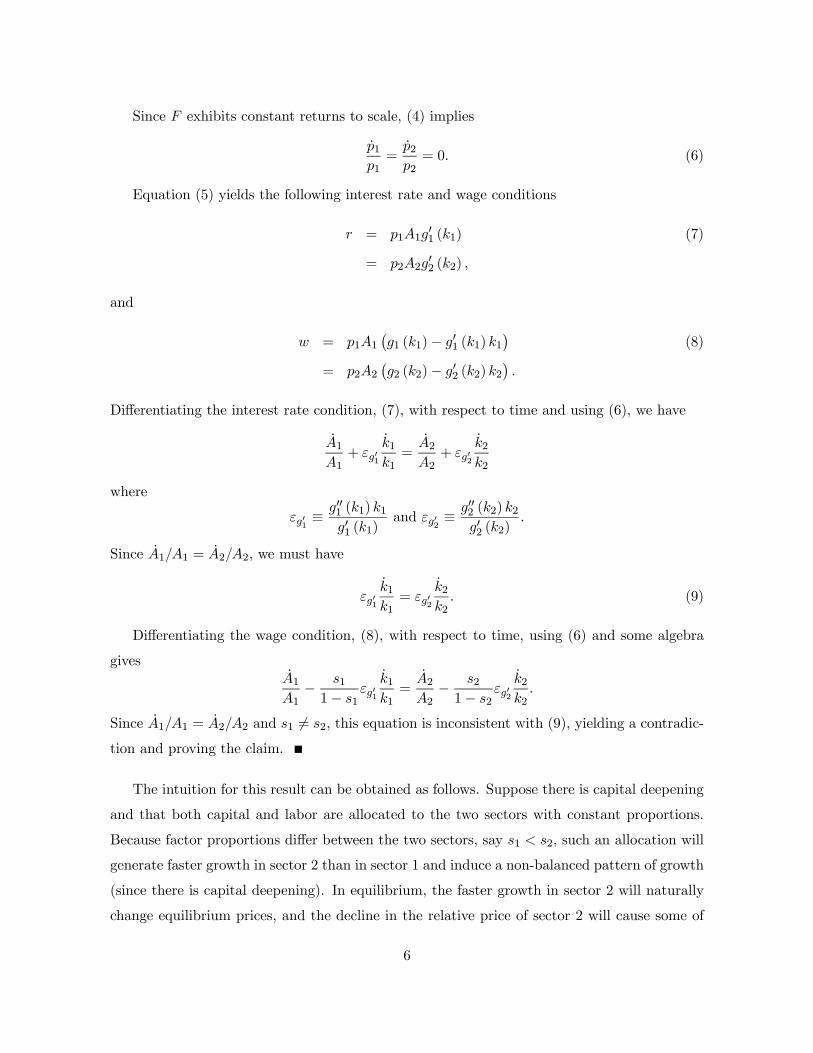
The equilibrium behavior of this economy can be represented by a system of autonomous

non-linear differential equations in three variables,

c ≡ C

LM1

α1(ν−1)1

, χ ≡ K

LM1

α1(ν−1)1

and κ.

Here c is the level of consumption normalized by population and technology (of the sector

which will dominate the asymptotic behavior), and is the only control variable; χ is the capital

stock normalized by the same denominator, and κ determines the allocation of capital between

the two sectors. These two are state variables with given initial conditions χ0 and κ0.14

The dynamic equilibrium conditions than translate into the following equations:

c

c=

1

θ

"(1− α1)

µν − 1ν

¶γ

µY

Y1

¶1ε

λα1 (κχ)−α1 − ρ

#− n− 1

α1 (ν − 1)m1, (52)

χ

χ= λα1κ1−α1χ−α1

µY

Y1

¶− χ−1c− n− 1

α1 (ν − 1)m1,

κ

κ=

(1− κ)h(α1 − α2)

χχ +

³1

ν−1

´³m2 − α2

α1m1

´i³

ε1−ε

´+ α2 + (1− α1) (1− κ) + (1− α2)κ+ (α1 − α2) (1− λ)

,

where µY

Y1

¶= γ

εε−1

∙1 +

µ1− α11− α2

¶µ1

κ− 1¶¸ ε

ε−1,

and

λ =

∙µ1− α1α1

¶µα2

1− α2

¶µ1− κ

κ

¶+ 1

¸−1.

Clearly, the constant growth path equilibrium characterized above corresponds to a steady-

state equilibrium in terms of these three variables, denoted by c∗, χ∗ and κ∗ (i.e., in the CGP

equilibrium, c , χ and κ will be constant). These steady-state values are given by κ∗ = 1,

χ∗ =

⎡⎣ν³θhn+ 1

α1(ν−1)m1

i+ ρ

´γ

εε−1 (1− α1) (ν − 1)

⎤⎦−1η

,

and

c∗ = γε

ε−1χ∗1−η − χ∗

µn+

1

α1 (ν − 1)m1

¶.

14χ0 is given by definition, and κ0 is uniquely pinned down by the static equilibrium allocation of capital attime t = 0, given by (32).

23

Since there are two state and one control variable, local (saddle-path) stability requires

the existence of a (unique) two-dimensional manifold of solutions in the neighborhood of the

steady state that converge to c∗, χ∗ and κ∗. The next theorem states that this is the case.

Theorem 4 The non-linear system (52) is locally (saddle-path) stable, in the sense that in

the neighborhood of c∗, χ∗ and κ∗, there is a unique two-dimensional manifold of solutions

that converge to c∗, χ∗ and κ∗.

Proof. Let us rewrite the system (52) in a more compact form as

x = f (x) , (53)

where x ≡¡c χ κ

¢0. To investigate the dynamics of the system (53) in the neighborhood

of the steady state, consider the linear system

z = J (x∗) z,

where z ≡ x− x∗ and x∗ such that f (x∗) = 0, where J (x∗) is the Jacobian of f (x) evaluated

at x∗. Differentiation and some algebra enable us to write this Jacobian matrix as

J (x∗) =

⎡⎣ acc acχ acκaχc aχχ aχκaκc aκχ aκκ

⎤⎦ ,where

acc = aκc = aκχ = 0

acχ = −γε

ε−1 (χ∗)−α1−1

µα1 (1− α1)

θ

¶µν − 1ν

¶acκ = γ

εε−1 (χ∗)

−α1µ1− α1

θ

¶µν − 1ν

¶ ∙µ1− α11− α2

¶µ1 + α2 (1− ε)

1− ε

¶− α1

¸aχc = − (χ∗)−1

aχχ = γε

ε−1 (χ∗)−α1−1

(1− α1)

∙1− 1

θ

µν − 1ν

¶¸+(χ∗)−1 ρ

θ

aχκ = γε

ε−1 (χ∗)−α1∙(1− α1) +

µ1− α11− α2

¶µ1 + α2 (1− ε)

1− ε

¶¸aκκ = −

µ1− ε

ν − 1

¶µm2 −

α2α1

m1

¶.

The determinant of the Jacobian is det (J (x∗)) = −aκκacχaχc. First, acχ and aχc are clearly

negative. Next, it can be seen that aκκ is always negative since we are in the case with

24

ε ≶ 1 ⇔ m2/α2 ≷ m1/α1.15 This implies that det (J (x∗)) > 0, so the steady state is

hyperbolic. Moreover, either all the eigenvalues are positive or two of them are negative and

one positive. To determine which is the case, we look at the characteristic equation given by

det (J (x∗)− vI) = 0, where v denote the eigenvalues. This equation is

(aκκ − v) [v (aχχ − v) + aχcacχ] = 0,

and shows that one of the eigenvalue is equal to aκκ and thus negative, so there must be

two negative eigenvalues. Consequently, there exists a unique two-dimensional manifold of

solutions in the neighborhood of this steady state, converging to it. This proves local (saddle-

path) stability.

This result shows that the constant growth path equilibrium is locally stable, and when

the initial values of capital, labor and technology are not too far from the constant growth

path, the economy will indeed converge to this equilibrium, with non-balanced growth at the

sectoral level and constant capital share and interest rate at the aggregate.

We next investigate the dynamics of some parameterized economies numerically. In par-

ticular, we wish to study the speed of convergence to the asymptotic equilibrium, and how the

economy behaves along the path of convergence, for example, whether the interest rate and

the share of capital change by large amounts along the transition path. Since the economy

with ε < 1 is our main focus, we only report simulations for this case.

Recall that our economy is fully characterized by ten parameters, γ, ε, ν, α1, α2, ρ, θ, n,

m1, and m2. We choose a period to correspond to a year, and take a baseline economy with

a 1% annual population growth (n = 0.01), ρ = 0.02 and θ = 2 as in the baseline calibration

of the neoclassical growth model in Barro and Sala-i-Martin (2004). We choose the rest of the

parameters to be consistent with 3% total growth rate of output (g = 0.03), a capital share

in national income of approximately 35% (sK = 0.35), and an interest rate of approximately

12% (r = 0.12).16 These choices imply that α1 ' 0.8 (essentially to match the share of capitalasymptotically), ε = 0.5 and ν ' 5 (to match the interest rate) and m1 ' 0.125 (to match thegrowth rate). Finally, in the benchmark simulation, we choose a capital intensity in sector 2

15As noted above, this is not a parameter restriction. When we have ε > 1 and m2/α2 > m1/α1, for example,then it will be sector 2 that grows more slowly in the limit, and stability will again obtain.16Since there is no depreciation in our model, the interest rate also corresponds to the rental rate of capital.

We choose 12% as the benchmark value to approximate a reasonable rental rate (e.g., an interest rate of 7%plus 5% depreciation).

25

close to that in sector 1, α2 = 0.75 and m2 = m1 ' 0.125 to highlight the non-balanced growthresulting from differential capital intensities in the two sectors. In addition, we choose a low

level of γ, γ = 0.15, to generate a fraction of employment in sector 1 of approximately 40%,

and the following initial values: L (0) = 1, K (0) = 1, ML (0) = 1 and MH (0) = 0.1.

Figure 1 shows the results of the simulations.17 The four panels depict λ, κ, the interest

rate (r) and the capital share (sK). The solid line is for the benchmark. The first remarkable

feature in the simulation is the rate of convergence. The units on the horizontal axis are years,

and range from zero to 3000. This shows that it takes a very very long time for the fraction

of capital and labor allocated to sector 1 to approach their asymptotic equilibrium value of 1.

For example, initially, about 40% of employment is in sector 1 and even after 500 years, less

than half of employment remains there. This illustrates that even though in the limit one of

the sectors employs all of the factors, it takes a very long time for the economy to approach

this limit point. Second, in the baseline simulation, the interest rate is essentially constant,

and varies only between 0.112 and 0.115 throughout the convergence process. The share of

capital in national income is declining visibly, but its range of movement is small (between

0.35 and 0.375). Moreover, in the first 500 years, the capital share essentially moves between

0.37 and 0.375). This is the basis of our claim that this type of model may lead to a pattern

of non-balanced sectoral growth (as shown by λ and κ in the top two panels), while generating

only small movements in the interest rate and the capital share, thus remaining approximately

consistent with the Kaldor facts.

17To perform the simulations, we first represent the equilibrium as a two-dimensional non-autonomous systemin c and χ (rather than the three-dimensional autonomous system analyzed above) since κ can be representedas a function of time only. This two dimensional system has one state and one control variable. FollowingJudd (1998, ch.10), we then discretize these differential equations using the Euler method, and turn theminto a system of first-order difference equations in ct and χt, which can itself be transformed into a second-order non-autonomous system only in χt. This second-order equation can be analyzed numerically by reversingtime, perturbing χ away from its steady-state value, and then integrating it backward to (χ0, κ0) (given theexogenously given sequence of state variables, {Lt,M1,t,M2,t}Tt=0 and boundary conditions χT+1 = χT = χ∗).

26

Figure 1. Solid line: α2 = .75. Dotted line: α2 = .72. Dashed line: α2 = .78.

The dashed and dotted lines in Figure 1 show variations with α2 = 0.78 and α2 = 0.72.

The dashed line shows that when α2 is increased even further, convergence is even slower, and

now after 3000 years only less than 70% of employment is in sector 1. Moreover, the interest

rate and the share of capital in national income are now essentially constant. When α2 is

reduced so that the gap between the capital intensity of the two sectors becomes larger, the

speed of convergence is a little faster, but is still very very slow. The range of change of the

capital share also becomes larger (between 0.35 and 0.39).

Figure 2 investigates the consequences of varying m2. The solid line is again for the

benchmark simulation, with m2 = m1 ' 0.125, while the dashed and the dotted lines show

simulations with m2 = 0.12 and m2 = 0.13. They show that when the TFP growth rate in the

capital-intensive sector is reduced, convergence takes much longer. For example, after 3000

years, a little above 60% of employment is in sector 1. The capital share also changes by very

27

little over this time period. In contrast, when the TFP growth rate of the capital-intensive

sector is increased, convergence is faster than the benchmark case but still very slow. For

example, it takes 2000 years for the share of employment in sector 1 to reach 90%. These

simulations therefore show that this class of economies may be able to generate significant

non-balanced sectoral growth, without substantially deviating from the Kaldor facts.

Figure 2. Solid line: m2 = .125. Dotted line: m2 = .12. Dashed line: m2 = .13.

4 Non-Balanced Endogenous Growth

In this section we introduce endogenous technological progress. This investigation is motivated

by two questions. As already emphasized, non-balanced growth results from capital deepening,

and so far, capital deepening was a consequence of exogenous technological change. The

first question is whether similar results obtain when technological change itself is endogenous.

Second and more important, one may wonder whether endogenous technological change will

28

take place in such a form as to restore balanced growth. The analysis in this section will

explicitly show that this is not the case. Finally, endogenizing technological change in this

context enables us to derive a model of non-balanced endogenous technological change, which

is an important direction for models of endogenous technology given the non-balanced nature

of growth in the data.

Demographics, preferences and technology are the same as described in the previous section,

except that instead of the exogenous processes for technology given in (18), we now need to

specify an innovation possibilities frontier, i.e., the technology to transform resources into

blueprints for new varieties in the two sectors. In particular, we assume that

M1 = b1M−ϕ1 X1 and M2 = b2M

−ϕ2 X2, (54)

where X1 ≥ 0 and X2 ≥ 0 are research expenditures in terms of the final good, b1 and b2 are

strictly positive constants measuring the technical difficulty of creating new blueprints in the

two sectors, and ϕ ∈ (−1,∞) measures the degree of spillovers in technology creation.18

Finally, we assume that there is free entry into research, and a firm that invents a new

intermediate of either sector becomes the monopolist producer with a perpetually enforced

patent. Given the value for being the monopolist for intermediate in (21), we have two free

entry conditions, which will pin down equilibrium technological change:

V1 ≤Mϕ1

b1and V2 ≤

Mϕ2

b2, (55)

with each condition holding as equality when there is positive R&D expenditure for that sector,

i.e., when X1 > 0 or X2 > 0.

The resource constraint of the economy is also modified to incorporate the R&D expendi-

tures,

K +C +X1 +X2 ≤ Y. (56)

Now a dynamic equilibrium is represented by paths of interest wages and rates, w and r,

labor and capital allocation decisions, λ and κ, satisfying (30) and (31), and of consumption,18When ϕ = 0, there are no spillovers from the current stock of knowledge to future innovations. With ϕ < 0,

there are positive spillovers and the stock of knowledge in a particular sector makes further innovation in thatsector easier. With ϕ > 0, there are negative spillovers (“fishing out”) and further innovations are more difficultin sectors that are more advanced (see, for example, Jones, 1995, Kortum, 1997). Similar to the results in Jones(1995), Young (1999) and Howitt (1999), there will be endogenous growth for a range of values of ϕ becauseof population growth. In the remainder, we will typically think of ϕ > 0, so that there are negative spillovers,though this is not important for any of the asymptotic results.Also, this innovation possibilities frontier assumes that only the final good is used to generate new technologies.

The alternative is to have a scarce factor, such as labor or scientists, in which case some amount of positivespillovers would be necessary.

29

capital stock, technology, values of innovation and research expenditures satisfying (21), (38),

(39), (54), (55) and (56). It is also useful to define a path that satisfies all of these equations,

possibly except the transversality condition, (39), as a quasi-equilibrium.

Since the case with ε < 1 is both more interesting, and in view of the discussion in footnote

2, also more realistic, in this section we focus on this case exclusively.

We first note that Propositions 1 and 2 from Section 3 still apply and characterize the

comparative static responses, and Lemmas 1 and 2 from there determine the behavior of the

growth rate of sectoral output, capital and employment. For the analysis of the economy

with endogenous technology, we also need an additional result in the next lemma. It shows

that provided that (i) ε < 1, (ii) there exists a constant asymptotic interest rate r∗ (i.e.,

limt→∞ r = 0), and (iii) there is positive population growth, in the asymptotic equilibrium the

free entry conditions in (55) will both hold as equality:

Lemma 3 Suppose that ε < 1, n > 0, and limt→∞ r = 0, then limt→∞ (V1 −Mϕ1 /b1) = 0 and

limt→∞ (V2 −Mϕ2 /b2) = 0.

The proof of this lemma is rather long and is provided in the Appendix.

This lemma is an important result for the analysis of non-balanced endogenous growth. It

enables us to solve for the asymptotic growth rates from the free entry conditions and obtain

a relatively simple characterization of the constant growth path equilibrium.

The economic intuition for the lemma comes from population growth; with population

growth, it is always optimal to allocate more capital to each sector, which increases the prof-

itability of intermediate producers in that sector. Consequently, the value of a new blueprint

increases asymptotically. This rules out asymptotic equilibrium paths with slack free-entry

conditions, because along such paths, the cost of creating a new blueprint would remain con-

stant, ultimately violating the free-entry condition.

To establish the existence of a CGP, we now impose the following parameter restriction,

which replaces (A2) in the exogenous technology case:

ζ > max

(1

α1,1

α1

∙1− (1− θ)

ρn

¸−1)(A3)

where ζ ≡ (ν − 1) (1 + ϕ). This assumption ensures that the transversality condition (39)

holds. Notice that in contrast to Assumption A2 only α1 features in this assumption, since,

given Assumption A1, α1 < α2 and with endogenous technology, this will make sure that sector

30

1 is the more slowly growing sector in the asymptotic equilibrium. Assumption A3 also rules

out quasi-equilibrium paths where output and consumption grow more than exponentially.

Lemma 4 Suppose Assumption A3 holds and ε < 1, then there exists no quasi-equilibria with

limt→∞ C/C =∞.

This lemma is proved in the Appendix, where, for completeness, we also show that As-

sumption A3 is “tight” in the sense that, if first inequality in this assumption, ζ > 1/α1, did

not hold, there always exist quasi-equilibria with more than exponential growth.

Combined Lemmas 3 and 4 imply that the asymptotic equilibrium has to converge either

to a limit with constant growth of consumption, or to a limit cycle. Using these results, the

next theorem establishes the existence of a unique constant growth path, with non-balanced

sectoral growth, but constant share of capital and constant interest rate in the aggregate. It

is therefore the analogue of Theorem 3 of the previous section, and is the main result of this

section.

Theorem 5 Suppose Assumptions A1 and A3 hold, ε < 1, and n > 0, then there exists a

unique CGP where

g∗ = g∗C = g∗1 = z∗1 =α1ζ

α1ζ − 1n, (57)

g∗2 =α1ζ (1− ε+ ζ) + εζ (α1 − α2)

(α1ζ − 1) (1− ε+ ζ)n > g∗, (58)

z∗2 =α1ζ (1− ε+ ζ)− ζ (α1 − α2) (1− ε)

(α1ζ − 1) (1− ε+ ζ)n < g∗, (59)

n∗1 = n and n∗2 =

∙1− ζ (1− ε) (α1 − α2)

(α1ζ − 1) [1− ε+ ζ]

¸n, (60)

m∗1 =1

1 + ϕz∗1 and m∗2 =

1

1 + ϕz∗2 . (61)

The proof of this theorem is also given in the Appendix.

There a number of important features worth noting. First, this theorem shows that the

equilibrium of this non-balanced endogenous growth economy takes a relatively simple form.

Second, given the equilibrium rates of technological change in the two sectors, m∗1 and m∗2,

the asymptotic growth rates are identical to those in Theorem 3 in the previous section, so

that the economy with endogenous technological change gives the same insights as the one

with exogenous technology. In particular, there is non-balanced sectoral growth, but in the

31

aggregate, the economy has a limiting equilibrium with constant share of capital in national

income and a constant interest rate. Finally, technology is also endogenously non-balanced,

and in fact, tries to counteract the non-balanced nature of economic growth. Specifically,

there is more technological change towards the sector that is growing more slowly (recall we

are focusing on the case where ε < 1), so that the sector with a lower share of capital has

an increasing share of capital, employment and technology in the economy. Nevertheless, this

sector still grows more slowly than the more capital-intensive sector, and the non-balanced

nature of the growth process remains. Therefore, endogenous growth does not restore balance

between the two sectors as long as capital intensity (factor proportion) differences between the

two sectors remain.19

5 Conclusion

This paper shows how differences in factor proportions across sectors combined with capital

deepening lead to a non-balanced pattern of economic growth. We first illustrated this point

using a general two-sector growth model, and then characterized the equilibrium fully using a

class of economies with constant elasticity of substitution between sectors and Cobb-Douglas

production technologies. This class of economies shows how the pattern of equilibrium may

be simultaneously consistent with non-balanced sectoral growth (the so-called Kuznets facts)

while also generating asymptotically constant share of capital in national income and interest

rate in the aggregate (the Kaldor facts). We also constructed and analyzed a model with

endogenous technology featuring non-balanced economic growth.

The main contribution of the paper is theoretical, but it also raises a number of empirical

questions. In particular, the analysis suggests that differences in factor proportions across

sectors will introduce a powerful force towards non-balanced growth, which could be important

in accounting for the cross-sectoral patterns of output and employment growth. Whether this

is so or not, especially in the context of the differential growth of agriculture, manufacturing

and services, appears to be a fruitful area for future research.

19Since there are two more endogenous state variables and two more control variables now, it is not possible toshow local stability analytically. In particular, in addition to c, χ and κ, we need to keep track of the endogenousevolution of M1, M2, X1 and X2 (or their stationary transformations). Given the size of this system, we areunable to prove local (saddle-path) stability.

32

6 Appendix

6.1 Proof of Proposition 2

Parts 1 and 2 follow from differentiating equation (36) and Proposition 1. Here we prove parts

3 and 4. Recall the expression for the equilibrium capital share

sK ≡rK

Y= 1− γα1

µY1Y

¶ ε−1ε

λ−1

with

λ =

∙µ1− η

1− α

¶µα

η

¶µ1

κ− 1¶+ 1

¸−1where combining the production function and the equilibrium capital allocation we get

µY1Y

¶ ε−1ε

=

"γ + (1− γ)

µY1Y2

¶1−εε

#−1

= γ−1µ1 +

µ1− α11− α2

¶µ1

κ− 1¶¶−1

Then, using the results of Proposition 1, we have

d ln sKd lnK

= −Sµ1− sKsK

¶µ1− α11− α2

¶(1− ε) (α1 − α2) (1− κ) /κ

1 + (1− ε) (α1 − α2) (κ− x)(62)

andd ln sKd lnM2

= − d ln sKd lnM1

= S

µ1− sKsK

¶µ1− α11− α2

¶(1− ε) (1− κ) /κ(ν − 1)

1 + (1− ε) (α1 − α2) (κ− x)(63)

where

S ≡"µ1 +

µ1− α11− α2

¶µ1

κ− 1¶¶−1

−µµ

α1α2

¶+

µ1− α11− α2

¶µ1

κ− 1¶¶−1#

with

S < 0⇔ α1 > α2.

This establishes the desired result that

d ln sKd lnK

< 0⇔ ε < 1

andd ln sKd lnM1

= − d ln sKd lnM2

> 0⇔ (α1 − α2) (1− ε) > 0.

¥

33

6.2 Proof of Lemma 3

We will prove this lemma in four steps.

Step 1: m∗1 = m∗2 = 0 imply g∗2 = g∗1 = n.

Step 2: lim supt→∞ (V1 −Mϕ1 /b1) ≥ 0 or lim supt→∞ (V2 −Mϕ

2 /b2) ≥ 0.Step 3: lim supt→∞ (V1 −Mϕ

1 /b1) ≥ 0 and lim supt→∞ (V2 −Mϕ2 /b2) ≥ 0.

Step 4: limt→∞ (V1 −Mϕ1 /b1) = 0 and limt→∞ (V2 −Mϕ

2 /b2) = 0.

Proof of Step 1: We first prove that m∗1 = m∗2 = 0 imply g∗2 = g∗1 = n. To see this,

combine equations (30) and (31) to obtainµY2Y1

¶ 1−εε

=

µ1− γ

γ

¶µ1− α21− α1

¶K1

K2.

Differentiating gives

1− ε

ε(α2n2 − α1n1) +

1− ε

ε(1− α2) z2 −

1− ε

ε(1− α1) z1 = z1 − z2. (64)

To derive a contradiction, suppose that g∗2 > g∗1. Then, from Lemma 1 n∗2 < n∗1 and z∗2 < z∗1

and from Lemma 2, g∗ = g∗1. Next, differentiating (25), we obtain

g1 = α1n1 + (1− α1) z1 +1

ν − 1m1 and g2 = α2n2 + (1− α2) z2 +1

ν − 1m2. (65)

Moreover, since limt→∞ r = 0, equation (41) and the fact that g∗ = g∗1 imply that g∗1 = z∗1.

This combined with equation (65) and m∗1 = 0 implies that z∗1 = n∗1 = n, which together with

(64) implies

0 >1− ε

ε(1− α2) (z

∗2 − z∗1) > z∗1 − z∗2 ,

yielding a contradiction. The argument for the case in which g∗2 < g∗1 is analogous. Since

g∗2 = g∗1 = g∗ and m∗1 = m∗2 = 0, it must also be the case that g∗2 = g∗1 = n, completing the

proof of step 1.

Proof of Step 2: First note that lim supt→∞ (V1 −Mϕ1 /b1) < 0 and

lim supt→∞ (V2 −Mϕ2 /b2) < 0 imply that the free entry conditions, (55), are asymptotically

slack, so m∗1 and m∗2 exist, and limt→∞m1 (t) = m∗1 = 0 and limt→∞m2 (t) = m∗2 = 0 (since

they cannot be negative). In particular, note that if lim supt→∞ (V1 −Mϕ1 /b1) < 0, this implies

that there exists no “infinitely-recurring” interval in the limit where the free entry condition

holds for sector 1.

34

Now to derive a contradiction, suppose that m∗2 = m∗1 = 0, which, as shown above, implies

g∗1 = g∗2 = g∗ = n > 0. Then, differentiating the second equation in (27), we obtain:

limt→∞

π2π2= g∗ > 0. (66)

Combining this with limt→∞ r = 0 and the value function in (21) yields: limt→∞ V2 = ∞.Since m∗2 = 0 by hypothesis, M

−ϕ2 is constant, and we have limt→∞ V2 =∞ > limt→∞Mϕ

2 /b2,

violating the free entry condition (55). This proves that m∗1 and m∗2 cannot both equal to 0,

and thus lim supt→∞ (V2 −Mϕ2 /b2) < 0 and lim supt→∞ (V1 −Mϕ

1 /b1) < 0 is not possible.

Proof of Step 3: We next prove that lim supt→∞ (V1 −Mϕ1 /b1) ≥ 0,

lim supt→∞ (V2 −Mϕ2 /b2) ≥ 0, lim supt→∞m1 > 0 and lim supt→∞m2 > 0.

Suppose, to derive a contradiction, lim supt→∞m2 = m∗2 = 0 and

lim supt→∞ (V2 −Mϕ2 /b2) < 0 (the other case is proved analogously). Since, as shown above,

m∗1 = m∗2 = 0 is not possible, we must have lim supt→∞ (V1 −Mϕ1 /b1) ≥ 0 and lim supt→∞m1 >

0.

We start by noting from (27), that asymptotically

limt→∞

π2π2=1

ε(g − g2) + g2, (67)

because m∗2 = 0. Since

limt→∞

r

r=1

ε(g − g2) + g2 − z2 = 0

from (31), z2 > 0 implies that limt→∞ π2/π2 > 0. But by the same argument as in Step 2, we

have limt→∞ V2 = ∞ > limt→∞Mϕ2 /b2, violating the free entry condition (55). We therefore

only have to show that z2 > 0 (i.e., lim supt→∞ z2 > 0). Suppose, to obtain a contradiction,

that z∗2 = 0. Using (40) and (41) from the proof of Lemma 1, we have z2 − n2 = z1 − n1,

which implies that n∗2 = 0 (recall that either n1 ≥ n or n2 ≥ n, and since limt→∞ g ≥ n, either

z1 ≥ n or z2 ≥ n). But then with n∗2 = z∗2 = m∗2 = 0, we have g∗2 = 0 < g∗1, which contradicts

n∗2 < n∗1 = n from Lemma 1. A similar argument for the other sector completes the proof that

lim supt→∞ (V1 −Mϕ1 /b1) ≥ 0 and lim supt→∞ (V2 −Mϕ

2 /b2) ≥ 0.

Proof of Step 4. From the free entry conditions in (55), we have that V1 −Mϕ1 /b1 ≤ 0

and V2 −Mϕ2 /b2 ≤ 0, thus lim supt→∞ (V1 −Mϕ

1 /b1) ≤ 0 and lim supt→∞ (V2 −Mϕ2 /b2) ≤ 0.

Combined with Step 3, this implies lim supt→∞ (V1 −Mϕ1 /b1) = 0 and

lim supt→∞ (V2 −Mϕ2 /b2) = 0. Hence, we only have to prove that lim inft→∞ (V1 −Mϕ

1 /b1) ≥ 0

35

and lim inft→∞ (V2 −Mϕ2 /b2) ≥ 0. We prove the first inequality (the proof of the second is

similar).

Suppose, to derive a contradiction, that lim inft→∞ (V1 −Mϕ1 /b1) < 0. This implies that

there exists a (recurring) interval (t00, t02) such that V1 (t) −Mϕ

1 (t) /b1 < 0 for all t ∈ (t00, t02).Suppose that (t00, t

02) is unbounded; this would imply that lim supt→∞m1 = m∗1 = 0, yielding a

contradiction with Step 1. Thus (t00, t02) must be bounded, so there exists (t0, t2) ⊃ (t00, t02) such

that for t ∈ (t0, t2) \ (t00, t02), we have V1 (t)−Mϕ1 (t) /b1 = 0. Moreover, since lim supt→∞m1 >

0, there also exists an interval (t000, t002) ⊃ (t0, t2) such that for all t ∈ (t0, t2) \ (t000, t002), m1 > 0.

Next, since m1 = 0 for all t ∈ (t00, t02), we also have M1 (t00) =M1 (t

02). This implies

V1¡t02¢=

Mϕ1 (t

00)

b1= V1

¡t00¢. (68)

Figure A1 shows this diagrammatically.

V1

M1φ/b1

t

M1φ/b1

V1

t0’’ t1’ t0’ t2’ t2’’

t0

Figure A1: The solid line represents Mϕ1 /b1 and the thick line represents V1.

Let us rewrite (21) in the Bellman equation form

V1 (t)

r= V1 (t)−

π1 (t)

r∀t. (69)

36

Equation (69) also shows that V1 (t) is well-defined, so V1 (t) is continuously differetiable in t.

Equation (68) and the fact that V1 (t) −Mϕ1 (t

00) /b1 < 0 for all t ∈ (t00, t02) imply that V1 (t)

reaches a minimum over (t00, t02) with V1 (t) = 0. Let t01 < t02 be such that V1 (t

01) is the first

local minimum after t00, which naturally satisfies V1 (t01) < V1 (t

00). Moreover, using (27) and

(31), we have that for all t

π1 (t)

r∗=

1

(ν − 1) (1− α1)

K1 (t)

M1 (t),

where r∗ = limt→∞ r (t) is the asymptotic equilibrium interest rate, which exists by hypothesis

that limt→∞ r (t) = 0. Also, using the fact that limt→∞ r (t) = 0 and the interest rate condition,

(30), we obtain that since m1 = 0 and n > 0, K1 (t01) > K1 (t

00). In addition, since M1 (t

01) =

M1 (t00), we can use (69) to write

V1 (t01)

r∗= V1

¡t01¢− 1

(ν − 1) (1− α1)

K1 (t01)

M1 (t01)< V1

¡t00¢− 1

(ν − 1) (1− α1)

K1 (t00)

M1 (t00)=

V1 (t00)

r∗< 0

which contradicts the fact that V1 (t01) is a local minimum, completing the proof of the lemma.¥

6.3 Proof of Lemma 4 and The Converse Result

Proof of Lemma 4: First, recall that C ≤ Y , (11). Hence it is enough to prove that

limt→∞ g =∞ will violate the resource constraint. We will prove this separately in two cases,

when g∗2 ≥ g∗1 and when g∗2 < g∗1

Suppose g∗2 ≥ g∗1 and g∗ = ∞. Then, Lemma 2 implies g∗1 = g∗ = ∞, and equation (41)together with (40) and (65) yields

g = n−µ1− α1α1

¶r

r+

1

α1 (ν − 1)m1.

Given n <∞ and limt→∞ r/r > 0, it must be that asymptotically

g∗ =1

α1 (ν − 1)m∗1. (70)

Combining the technology possibility frontier (54) and (70) we have

limt→∞

X1

X1= lim

t→∞m1

m1+ α1 (1 + ϕ) (ν − 1) g∗.

Then, the first inequality in Assumption A3, ζ > 1/α1, implies

limt→∞

X1

X1> g∗,

37

which violates the resource constraint (13).

Next suppose that g∗1 > g∗2and g∗ = ∞. Then, following the steps of above, Lemma 2implies g∗2 = g∗ =∞, and equation (41) together with (40) and (65) yieldsµ

1− α1 (1− ε)

ε

¶g1 = α1n1 +

µ1− α1

ε

¶g − (1− α1)

r

r+

µ1

ν − 1

¶m1.

Since g∗ = ∞ , a fortiori g∗1 = ∞, and, given n < ∞ and limt→∞ r/r > 0, we have that

asymptotically

m∗1 = (ν − 1)∙µ1− α1 (1− ε)

ε

¶g∗1 −

µ1− α1

ε

¶g∗¸. (71)

Once again the innovation possibilities frontier (18) implies

limt→∞

X1

X1= lim

t→∞m1

m1+ α1 (1− ϕ)m∗1.

Then equation (70) together with the first inequality in Assumption A3, ζ > 1/α1, implies

limt→∞

X1

X1> α1 (1− ϕ) (ν − 1) g∗ > g∗,

which violates the resource constraint (13), completing the proof that when Assumption

A3 holds any quasi-equilibrium with more than exponential growth violates the resource

constraints.¥

For completeness, we also prove the converse of Lemma 4, which shows that the use of the

first inequality in Assumption A3, ζ > 1/α1, in this lemma is “tight” in the sense that, if it

were relaxed, the converse result would obtain.

Lemma 4’: Suppose A1 holds, but ζ ≡ (ν − 1) (1− ϕ) ≤ 1α1, then there exists quasi-

equilibria with limt→∞ g =∞.Proof. This lemma will be proved by showing that in this case

g∗2 = g∗1 = g∗ =∞ and z∗2 = z∗1 = z∗ (72)

z∗ = g∗ − r

r(73)

m1

m1=

m2

m2= [1− α1ζ] g (74)

is a quasi-equilibrium.

From the interest rate conditions in the two sectors (30) and (31), and (72) we obtain

z∗ = g∗ − limt→∞

r

r

38

which is exactly condition (73). By substituting into (65), we obtain

g∗ = n1 −µ1− α1α1

¶limt→∞

r

r+

1

α1 (ν − 1)m∗1

g∗ = n2 −µ1− α2α2

¶limt→∞

r

r+

1

α2 (ν − 1)m∗2

which gives g∗ = 1α1(ν−1)m

∗1 and g∗ = 1

α2(ν−1)m∗2, and hence

m∗1 =α1α2

m∗2.

Differentiating this condition gives equation (74).

Finally, we need to check feasibility, i.e., that the R&D expenditures do not grow faster

than output. From the technology possibilities frontiers, (18), this requires

limt→∞

X1X1

=m∗1m∗1

+ α1ζg∗ ≤ g∗

limt→∞

X2X2

=m∗2m∗2

+ α2ζg∗ ≤ g∗

and both these conditions are satisfied given (74) and α1 > α2.

6.4 Proof of Theorem 5

We prove this proposition in two steps.

Step 1: Provided that g∗2 ≥ g∗1 > 0, then there exists a unique CGP defined by equations

(57), (58), (59), (60) and (61), satisfying g∗2 > g∗1 > 0.

Step 2: All CGP must satisfy g∗2 ≥ g∗1 > 0.

Proof of Step 1. Lemma 3 establishes that as t→∞ the free-entry conditions (55) must

asymptotically hold as equality. Combining (55) as equality with (69) (and the equivalent for

sector 2), we obtain the following conditions that must hold as t→∞:

γν

¡Y1Y

¢− 1ε Y1

r − ϕm1=

M1+ϕ1

b1and

γν

¡Y2Y

¢−1ε Y2

r − ϕm2=

M1+ϕ2

b2(75)

Differentiating (75) yields:

g1 −1

ε(g1 − g)− (1 + ϕ)m1 = 0 and g2 −

1

ε(g2 − g)− (1 + ϕ)m2 = 0. (76)

39

Then g∗2 > g∗1 > 0 and Lemma 2 imply that we must also have g∗ = g∗1. This condition together

our system of equations, (40), (41), (65), (76), solves uniquely for n∗1, n∗2,z

∗1, z

∗2 , m

∗1, m

∗2, g

∗1

and g∗2 (and κ∗ = λ∗ = 1) as given in equations (57), (58), (59), (60) and (61). Note that

this solution is consistent with g∗2 > g∗1 > 0, since Assumptions A1 and A3 immediately imply

that g∗2 > g∗1 and g∗1 > 0 (which is also consistent with Lemma 3). Finally, C ≤ Y , (11) and

(39) imply that the consumption growth rate, g∗C , is equal to the growth rate of output, g∗.

Finally, we can verify that an equilibrium with κ∗, λ∗, n∗1, n∗2, z

∗1 , z

∗2 , m

∗1, m

∗2, g

∗1 and g∗2

satisfies the transversality condition (39) with a similar argument to the one spelled in the first

step of the proof of Theorem 3.

Proof of Step 2. The proof that along all CGPs g∗2 > g∗1 > 0 must be true, is analogous

to the one of the second step in the proof of Theorem 3.¥

40

References

[1] Acemoglu, Daron, “Directed Technical Change” Review of Economic Studies, LXIX

(2002b), 781-810.

[2] Acemoglu, Daron, “Labor- and Capital-Augmenting Technical Change” Journal of Euro-

pean Economic Association, I (2003), 1-37.

[3] Aghion, Philippe and Peter Howitt, “A Model of Growth Through Creative Destruction”

Econometrica, LX (1992), 323-351.

[4] Aghion, Philippe and Peter Howitt, Endogenous Growth Theory, Cambridge, MA, MIT

Press, 1998.

[5] Antras, Pol, “Is the U.S. Aggregate Production Function Cobb-Douglas? New Estimates

of the Elasticity of Substitution” MIT mimeo (2001).

[6] Barro, Robert and Xavier Sala-i-Martin. Economic Growth, McGraw Hill, New York

(2004, 2nd edition).

[7] Baumol, William J., “Macroeconomics of Unbalanced Growth: The Anatomy of Urban

Crisis”, American Economic Review, LVII (1967), 415-426.

[8] Berndt, Ernst, “Reconciling Alternative Estimates of the Elasticity of Substitution,” Re-

view of Economics and Statistics, LVIII (1976), 59-68.

[9] Caselli, Francesco and Jaume Ventura “A Representative Consumer Theory of Distribu-

tion” American Economic Review, XC (2000), 909-926.

[10] Caselli, Francesco and John Coleman, “The U. S. Structural Transformation and Regional

Convergence: a Reinterpretation” Journal of Political Economy CIX (2001) 584-617.

[11] Chenery, Hollis, “Patterns of Industrial Growth”, American Economic Review, V (1960),

624-654.

[12] Chirinko, Robert S. “Business Fixed Investment: a Critical Survey of Modeling Strategies,

Empirical Results and Policy Implications” Journal of Economic Literature, XXXI, (1993),

1875-1911.

41

[13] Chirinko, Robert S., Steven M. Fazzari and Andrew P. Mayer, “How Responsive Is Busi-

ness Capital Formation to Its User Cost?” Journal of Public Economics, LXXV, (1999),

53-80.

[14] David, Paul, and Th. Van de Klundert, “Biased Efficiency Growth and Capital-Labor

Substitution in the U.S., 1899-1960,” American Economic Review, LV, (1965), 357-393.

[15] Denison, Edward F, “Accounting for United States Economic Growth, 1929-1969” Wash-

ington, DC: Brookings Institution (1974).

[16] Echevarria, Cristina, “Changes in Sectoral Composition Associated with Economic

Growth”, International Economic Review, XXXVIII (1997), 431-452.

[17] Gollin, Douglas, Stephen Parente and Richard Rogerson “The Role of Agriculture in

Development” American Economic Review Papers and Proceedings XCII (2002) 160-164.

[18] Griffin, James M. and Paul R. Gregory, “An Intercountry Translog Model of Energy

Substitution Responses”, American Economic Review, LXVI (1976), 845-857.

[19] Grossman, Gene and Elhanan Helpman, “Quality Ladders in the Theory of Growth”

Review of Economic Studies, LIIX (1991a), 43-61.

[20] Grossman, Gene and Elhanan Helpman, Innovation and Growth in the Global Economy,

Cambridge, MA, MIT Press, 1991b.

[21] Hamermesh, David S., Labor Demand, Princeton University Press, Princeton 1993.

[22] Howitt, Peter, “Steady Endogenous Growth with Population and R&D Inputs Growing”

Journal of Political Economics, CVII (1999), 715-730.

[23] Jones, Charles I., “R&D-Based Models of Economic Growth”, Journal of Political Eco-

nomics, CIII (1995), 759-784.

[24] Jones, Charles I., “The Shape of Production Functions and the Direction of Technical

Change”, U.C. Berkeley mimeo (2004).

[25] Judd, Kenneth, Numerical Methods in Economics, MIT Press, Cambridge, 1998.

42

[26] Kaldor, Nicholas , “Capital Accumulation and Economic Growth”, in Friedrich A. Lutz

and Douglas C. Hague, eds., Proceedings of a Conference Held by the International Eco-

nomics Association, London, Macmillan.(1963)

[27] Kongsamut, Piyabha , Sergio Rebelo and Danyang Xie, “Beyond Balanced Growth”,

Review of Economic Studies, LXVIII (2001), 869-882.

[28] Kortum, Samuel, “Research, Patenting and Technological Change” Econometrica, LXV

(1997), 1389-1431.

[29] Krusell, Per; Lee Ohanian and Victor Rios-Rull and Giovanni Violante, “Capital Skill

Complementary and Inequality”, Econometrica, LXIIX (2000), 1029-1053.

[30] Kuznets, Simon, “Quantitative Aspects of the Economic Growth of Nations: II, Indus-

trial Distribution of National Product and Labour Forcce”, Economic Development and

Cultural Change, V Supplement (1957).

[31] Kuznets, Simon, “Modern Economic Growth: Findings and Reflections”, American Eco-

nomic Review, LXIII (1973), 829-846.

[32] Laitner, John, “Structural Change and Economic Growth”, Review of Economic Studies,

LXVII (2000), 545-561.

[33] Lucas, Robert E., “On the mechanics of economic development.” Journal of Monetary

Economics , XXII (1988), 3-42.

[34] Matsuyama, Kiminori, “Agricultural Productivity, Comparative Advantage and Economic

Growth” Journal of Economic Theory LVIII (1992), 317-334.

[35] Matsuyama, Kiminori, “Structural Change” forthcoming New Pelgrave Dictionary of Eco-

nomics (2005).

[36] Mairesse, Jacques, Bronwyn H. Hall and Benoit Mulkay, “Firm-Level Investment in France

and the United States: An Exploration over What We Have Returned in Twenty Years”

Annales d’Economie et Statistiques, LV (1999), 27-67.

[37] Murphy, Kevin, Andrei Shleifer and Robert Vishny, “Income Distribution, Market Size

and Industrialization” Quarterly Journal of Economics CIV (1989), 537-564.

43

[38] Nadiri, M. I. “Some Approaches to Theory and Measurement of Total Factor Productivity:

a Survey” Journal of Economic Literature, VIII, (1970), 1117-77.

[39] Nerlove, Mark, “Recent Empirical Studies of the CES and Related Production Functions”

in M. Brown (editor) The Theory and Empirical Analysis of Production New York (1967).

[40] Ngai Rachel and Christopher Pissarides (2005), “Structural Change in a Multi-Sector

Model of Growth”, mimeo.

[41] Romer, Paul M., “Increasing Returns and Long-Run Growth” Journal of Political Econ-

omy, XCIV (1986), 1002-1037.

[42] Romer, Paul M., “Endogenous Technological Change” Journal of Political Economy, IIC

(1990), S71-S102.

[43] Segerstrom, Paul S., T. C. A. Anant, and Elias Dinopoulos, “A Schumpeterian Model of

the Product Life Cycle” American Economic Review LXXX (1990), 1077-1092.

[44] Young, Alwyn “Invention and Bounded Learning by Doing” Journal of Political Economy

CI (1993), 443-472.

[45] Young, Alwyn “Growth without Scale Effect” Journal of Political Economy, CVI (1998),

41-63.

44