CAPITAL CONTROLS IN BRAZIL: EFFECTIVE?

Marcos Chamon and Márcio Garcia1

September 11, 2013

Abstract

Controls on capital inflows gained new respectability as a macroprudential tool to preserve financial stability. In the aftermath of the 2008 great crisis, capital poured in emerging markets, enticing many different reactions. No emerging market experimented more with capital controls than Brazil during that period. We analyze the impact of the controls and restrictions on capital inflows that Brazil has adopted since late 2009. We document that these policies had some success in segmenting the Brazilian from global financial markets, as measured by the spread between onshore and offshore dollar interest rates, as well as ADR premia relative to the underlying local stocks. However, that failed to translate into significant changes in the exchange rate, at least in the immediate aftermath of these measures, suggesting limited success in mitigating exchange rate appreciation. Even if we treat the estimated effects as permanent, the 12 measures considered would have depreciated the Brazilian real by only 5 percent. Capital controls may have prevented a credit bubble, but they raised the cost of capital and, at most, had a limited effect on the exchange rate. JEL Codes: F31, F32, F36 and F65 Keywords: Capital Controls, Capital Flows, Macroprudential Policies, Exchange Rate, Brazil

1 Chamon: Research Department, International Monetary Fund, mchamon@imf.org; Garcia: Visiting Scholar at the Sloan School, MIT, and NBER, and Associate Professor at the Department of Economics, PUC-Rio, mgarcia8@mit.edu. The views expressed are those of the authors and should not be attributed to the IMF or any other institution. We thank BM&F Bovespa for data; many traders for enlightment of the pratical implications of the controls; and Stijn Claessens, Mercedes Garcia-Escribano, José de Gregorio, Anton Korinek, Marcelo Medeiros, Hyun Shin, Tony Volpon, Kristin Forbes and seminar participants at the 2013 ASSA meetings, the IMF, the Institute for Latin American Studies at Columbia University, the Center for International Development at Harvard University, and the REAP-INSPER conference for comments. Diego Barrot, Julia Bevilaqua, Hyeon Ji Lee, Felipe Lima, Guilherme Lima, and Guido Maia provided excellent research assistance. Márcio Garcia thanks CNPq and FAPERJ (Brazil) for financial support. Any errors are our own.

2

I. INTRODUCTION

Emerging markets have experienced a strong recovery in capital inflows in the aftermath of the systemic sudden stop in late 2008-early 2009. Flows reached levels comparable to their pre-crisis peak, driven by a combination of relatively favorable fundamentals in emerging markets and a “search for yield” in the context of low interest rates in advanced economies. These flows should, in principle, bring numerous benefits, helping finance investment opportunities that may be otherwise missed, smoothing shocks to consumption and facilitating technology transfers in the case of FDI. But they can also bring risks. One concern is that massive inflows can lead to a strong appreciation of the exchange rate and loss of competitiveness of the tradable sector. Given large adjustment costs, a strong but temporary appreciation may cause lasting damage to industries which may not recover even after the flows abate and the exchange rate returns to its equilibrium level. Large inflows can also complicate macroeconomic management by further stimulating an already overheating economy, particularly if efforts to control inflation through higher interest rates attract more inflows. On the prudential side, there are concerns that flows may be associated with risky external liability structures, and more generally that the flows may not be directed to productive uses, and end-up fueling consumption booms and asset price bubbles instead. Emerging markets have been aware of these risks from previous surge episodes, but the Global Financial Crisis has heightened these concerns. Recent papers have shown capital controls may play a useful role in managing the macroeconomic and prudential risks associated with flows (e.g. Ostry et al 2010, 2012, Korinek 2011, Rey 2013 and Engel 2013). There has been a marked change in the conventional wisdom among policy makers, with the IMF recognizing capital controls as a valid component of the policy toolkit under appropriate circumstances (IMF 2012). Brazil has been one of the leading countries in this effort to manage inflows, and one of the most vocal against the loose monetary policy in advanced economy policies that are pushing capital towards emerging markets (the Brazilian finance minister, Guido Mantega, coined the term “currency wars”). It sought to limit inflows in the aftermath of the crisis, adopting taxes on portfolio inflows in October 2009. Over the following two years, Brazil adopted a series of other measures to discourage inflows, starting gradually to dismantle them in 2012. In this paper, we document that these efforts had some success in segmenting Brazil’s domestic financial market from the global one, and analyze the impact of these measures on the exchange rate. The controls on capital inflows further segmented the Brazilian from global financial markets, as measured by wedges between onshore and offshore prices of similar fixed and variable income assets. Nevertheless, there is little effect on the exchange rate following most measures. Even if we treat all of the estimated effects as permanent, the 12 capital control/restriction measures deployed over the course of two and a half years would have only

3

depreciated the exchange rate by about 5 percent. While the exchange rate seems to revert from an appreciation trend following some measures, we do not find significantly strong effects on specifications that consider longer time windows. It is possible that measures were adopted during times of unusually favorable global financial conditions (and hence tend to be in the vicinity of local peaks of the exchange rate), a hypothesis that is supported by a similar behavior similar for other emerging market currencies around those dates. There is a vast literature on the effect of capital controls on the exchange rate. Magud, Reinhart and Rogoff (2011) provide an excellent survey and meta-analysis of that literature. The evidence on the effectiveness of controls on reducing the volume of flows, and hence exchange rate pressures, is mixed. The evidence tends to be stronger for an effect on the composition of flows (e.g. controls on portfolio flows leading to a shift towards FDI or longer maturities for which the control is less burdensome). Part of this shift may just reflect a relabeling of flows. Controls can also have an effect on financial stability (Jinjarak et al 2012, Ostry et al 2012). Klein (2012) distinguishes between permanent and transitory controls (“walls and gates”), concluding that the latter are not very effective in affecting macroeconomic variables. Several studies have focused on specific country experiences with controls. Some noteworthy capital controls on inflows in Latin America include the Chilean Unremunerated Reserve Requirement (URR) adopted in 1991-98, and the Colombian URR adopted in 1993-98 and 2007-08. De Gregorio, Edwards and Valdes (2000) who show that the Chilean (URR) had a very small effect on the real exchange rate, but was more successful in tilting the composition of flows towards longer maturities. Edwards and Rigobon (2009) find a stronger (but still modest) effect of the controls on the exchange rate. Forbes (2007) analyzes the potential costs of the Chilean controls, finding that they increased financing costs, particularly for small and medium enterprises.2 Cardenas and Barrera (1997) show that the Colombian URR in the 1990s did not affect the volume of flows, but had some success in shifting foreign liabilities towards longer-term maturities. Clements and Kamil (2009) find that the 2007-08 Colombian URR did not have a significant impact on the volume of non-FDI flows, and did not moderate exchange rate pressures. While most studies tend to focus on macroeconomic and financial stability outcomes, one should bear in mind that benefits should be weighed against costs. In the Brazilian context, Cardoso and Goldfajn (1997) show the capital controls were only effective in restricting financial inflows to Brazil in the 1990s for two to six months. Carvalho and Garcia (2008) present strong evidence that the controls had been bypassed during the first years after the end of hyperinflation (1994), when a combination of controlled exchange rate 2 Korinek (2011) argues that a successful and welfare increasing prudential regulation, which deters over borrowing, should precisely increase debt costs. But while risky external liability structures can lead to crises, they can also lead to higher growth in tranquil times (Ranciere, Tornell, and Vamvakidis 2010).

4

with extremely high interest rates attracted much carry-trade. Benelli, Segura-Ubiergo and Walker (2011) describe some of the recent measures adopted by Brazil to manage capital inflows, discussing the evolution of flows, domestic financial market developments and the exchange rate. Jinjarak et al (2013) use a synthetic cohort approach to study some of the recent Brazilian controls, and find that the restrictions did not affect flows or the exchange rate. While their approach allows for a counter-factual exchange rate to be constructed based on the evolution of the exchange rate in other countries, it does not allow for other explanatory variables (including Brazil-specific variables) that could affect the exchange rate to be considered.3 In a contemporaneous paper, Baumann and Gallagher (2012) also find that the Brazilian controls had a significant but small effect on the exchange rate. The recent Brazilian experience provides an ideal context to study the effect of capital controls and restrictions. No other country with a similar level of openness has ever experimented as actively with market-based capital controls, placing Brazil on a category of its own.4 Our study adds value to the literature on controls for a number of reasons. It provides the most detailed and in depth discussion of the policies adopted and their effect on domestic financial markets. Brazil has very sophisticated capital markets (arguably the most sophisticated among emerging markets), with deep and liquid instruments which we use to document the effectiveness of capital controls in segmenting the domestic and global markets. The measures adopted were transparent and market-based. The inflow tax increases were announced when the market was closed and became effective on the following day, so are particularly suitable for daily-frequency analysis. We use daily data and control for a host of variables that can also affect the exchange rate, including daily sterilized intervention data (not only through spot interventions but also through futures and swaps), and also test the effect of controls over longer horizons. The remainder of the paper is organized as follows. Section II describes the history of capital controls in Brazil. Section III analyzes the effectiveness of these controls in Brazil, since 2009. It shows how the controls create wedges between prices onshore and offshore, both on the fixed income, and on the variable income markets. Then, it analyzes whether or not the controls were able to mitigate the nominal appreciation of the real. Finally, Section IV presents the conclusions and the policy implications of our findings.

3It is also difficult to recover an intuition for the results, since as pointed out in their paper, the country weights on the synthethic cohort have no economic significance or otherwise interpretable meaning.

4 In the preface of their book “Who needs to open the capital account?” (Jeanne et al. 2012), the authors name only two countries, China and Brazil, the first as a country that maintains tight restrictions on its capital account, and Brazil as a country that has actively experimented with market-based prudential capital controls since the crisis.

5

II. CAPITAL CONTROLS IN BRAZIL

Controls on capital outflows have a long history in Brazil, since financial repression was the norm until the early 1990s. In 1991, real interest rates were significantly raised to avoid capital flight and help to accumulate foreign reserves. With the low rates prevailing in the US, capital started flowing in the country. So much so, that, starting in 1993, controls on capital inflows were enacted. Unlike the Chilean or Colombian capital controls, which took the form of unremunerated reserve requirements, the capital controls in Brazil took the form of a tax on the exchange rate transaction when capital first entered Brazil. This tax was a particular stance of the IOF tax, which taxes most financial transactions in Brazil with different tax rates (IOF is the Portuguese acronym for Tax on Financial Transactions).Most countries tend to use unremunerated reserve requirements instead of taxes to discourage inflows because the latter typically requires congressional approval. Brazil’s case is unique because the inflow tax already existed, and the Executive can change its rate by decree (including setting it to zero) without congressional approval. During the nineties, the top IOF tax rate on capital inflows applied to fixed income (carry-trade) was 9%.5 With the capital flight caused by the Russian crisis and the LTCM debacle, in 1998, the IOF tax rate on capital inflows was set to zero. In 2008, it was again raised to 1.5% for a brief period as a way (albeit imperfect) to equalize the tax treatment of foreigners (who were not subject to the income tax imposed on domestic investors). This IOF was removed when the capital flight associated with the Lehman crisis began. With the resumption of massive capital inflows, as early as February 2009, capital inflows were again deployed. Table 1 lists the measures that have been adopted in Brazil since October 2009, which are the subject of the current paper. All the IOF tax increases and restrictions listed in that table were announced when the Brazilian market was closed and became effective at the time of their publication (next business day).6 On October 19th, 2009, a tax of 2 percent was imposed on portfolio flows, covering both equities and fixed income. In the past, equity flows were often excluded from such taxes. Unlike the opportunistic and volatile carry-trade, equity flows are typically perceived to be a fairly safe type of flow. Nevertheless, Brazilian equity markets attracted so much capital in the aftermath of the recovery from the Global Financial Crisis that the government, concerned with the exchange rate appreciation, decided to include stocks in the controls. Also, the use of stocks as a vehicle to bring funds in the country aiming to replicate 5 Carvalho and Garcia (2008) describe several ways through which the IOF tax was avoided at the time. Cardoso and Goldfajn (1998) also measure the effectiveness of those taxes.

6 The only restriction in that table that did not become effective on the following business day was the URR on the Bank’s Gross FX Position announced on January 6, 2011, which only became effective on April 4, 2011. In contrast, the tightening of that URR announced on July 8, 2011 became effective on the following business day.

6

fixed income returns, as had happened in the previous Brazilian experience with controls on capital inflows, in the 1990s (discussed in Carvalho and Garcia 2008), may have played a role. One obvious channel, which allowed investors to bypass the controls in the case of equity flows, was the conversion of Depositary Receipts (DRs). DRs are securities issued by a custodian bank, which buys the underlying stock in Brazil, and issues a corresponding stock that is traded in foreign markets (e.g. ADRs in the case of U.S. markets). On November 18, 2009 a 1.5 percent tax was imposed on the issuance of DRs to discourage their use as a way to buy Brazilian equities without incurring the inflow tax. When a foreign investor buys a DR, it has the right to convert that DR into the underlying stock in the Brazilian market. This provided a mechanism to enter the Brazilian financial market without incurring the 2 percent tax on capital inflows. Eventually a tax of 2 percent was imposed on those conversions (December 30, 2010). There were no other changes targeting equity inflows, and taxes on equity flows were eventually removed (set to zero) on December 2011, although the 1.5% IOF tax on DR issuance still remains. The fixed income arena has seen much more regulatory action, as a series of measures tightened restrictions on fixed income flows. The tax on fixed income flows, initially set at 2%, was raised to 4%, on October 4th 2010, and shortly afterwards to 6%,on October 18th, 2010. The controls discriminate against only a subset of capital inflows (portfolio flows), leaving others untaxed. If a transfer between a financial institution abroad and its domestic counterpart could fall in the non-taxed subset it would not incur the IOF tax. Therefore, foreign investors wanting to do carry trade could buy Non-Deliverable Forward Brazilian reals in offshore markets (where they are beyond the reach of the inflow tax), and the banks could take an offsetting position in Brazil. The end result would be banks selling dollars to the Brazilian Central Bank for reals in order to offset the position (which causes the same pressure on the exchange rate as if the foreigners had come directly). It is difficult to gauge how much such strategies have been used during the last episode of capital controls. On January 6th, 2011, an unremunerated reserve requirement was imposed on banks’ gross FX liabilities beyond US$ 3 billion (on the spot market only),7 which limited the extent to which the strategy described above could be used to bypass the controls. On March 28th, 2011, Brazilian

7 In Brazil, only banks with a special charter granted by the central bank may trade in the spot exchange rate market. This hindrance has historically stimulated the use of exchange rate derivatives, as discussed in Ventura and Garcia (2011). Also, banks’ assets and liabilities in foreign currency have always been closely monitored by the Brazilian Central Bank, and very often controlled. In times of massive capital inflows, restrictions on banks’ liabilities are usually deployed, as exemplified by this unremunerated reserve requirement. On the other extreme, i.e., in times of capital flight, limits to FX assets were typically imposed. This is because increases in banks’ FX liabilities bring liquidity, while increases in banks’ FX assets drain liquidity from the domestic FX market.

7

firms borrowing abroad became subject to a 6 percent tax on those flows if their maturity was less than 1 year (extended to two years shortly afterwards). Related measures were adopted to prevent firms from borrowing abroad long-term without paying the tax and then converting the loan to a shorter maturity. Foreign investors could use derivatives to leverage their currency exposure, with the inflow tax only being applied to the money they brought to Brazil to meet their margin requirements. Such strategies were somewhat constrained by the earlier measure restricting banks’ gross spot FX positions (which was further tightened on July 8th, 2011). And on July 26th, 2011 a tax on the notional amounts of currency derivatives was introduced. The initial tax rate being set at 1 percent, and the maximum rate being set at 25% (although the rate was never actually raised). This tax is levied whenever a currency derivative is purchased, sold, or at its expiration date (and therefore investors are exposed to the risk that the tax rate increases while they are holding the derivative). On February and March 2012, additional restrictions were put in place (limiting the anticipation of payments to exporters, and extending the tax on foreign borrowing to loans with maturities up to 3 years, and then up to 5 years). During 2012, capital flows to Brazil waned. Also, the real depreciated much more than other similar currencies, prompting inflationary concerns, especially after the large reduction of the policy interest rate by the Brazilian Central Bank. By the end of 2012, a movement to withdraw some of the capital controls started, aimed at attracting capital inflows, as the Brazilian central bank started providing U.S. dollars through repo operations (which has a similar effect to sterilized sales of foreign exchange), so as to manage the exchange rate (which hovered around a relatively narrow band above 2 BRL/USD from May/2012 to May/2013, with relatively small volatility). The tax on foreign borrowing was limited to loans with maturities up to 2 years on June 2012, and eventually limited to loans with maturities up to 1 year in December 2012. On June 4, 2013, amid concerns about excessive weakening of the Brazilian real, the tax on fixed income flows was eliminated (set to zero). Eight days later, the IOF tax on the notional amount of currency derivatives was also eliminated (set to zero). As of the time of writing, the only remaining restrictions are the 6% tax on short term external loans (maturity less than a year), and the 1.5% tax on issuances of DRs.

III. EFFECTIVENESS OF MEASURES

Figure 1 reports the gross capital inflows to Brazil broken down by different types of flows (monthly data). We observe sizable inflows in the period prior to the Global Financial Crisis, with a sharp reversal in late 2008/early 2009 (with the exception of FDI flows which remained positive even at the height of the crisis). But inflows recover rapidly following the crisis, and by mid-2009 inflows are comparable to their pre-crisis levels. The first vertical line indicates the imposition of the 2 percent tax on portfolio flows. Both portfolio equity and debt flows remain strong after the imposition of that tax. The second vertical line indicates the month when the tax on portfolio debt inflows was raised to 4 and then to 6 percent. While portfolio debt flows decline following the increase in the tax, they continue to trickle. Perhaps the most striking

8

pattern in Figure 1 is the sizable increase in FDI flows during this period. While there was indeed much FDI during this period, this shift could partly reflect a relabeling of flows as FDI so as to avoid the inflow tax. One often hears the argument that intra-company loans are classified as foreign direct investment, thereby avoiding the IOF tax. We checked with the Brazilian Central Bank whether this was the case. According to the explanation given to us, the classification of intra-company loans as FDI is solely for statistical purposes. Intra-company loans were taxed at the same rate as regular (non-intra-company) loan with the same characteristics. According to this explanation, it is very hard to avoid the taxes by relabeling flows.8Nevertheless, financial institutions that operate both in Brazil and abroad seem to have more room to avoid the IOF, offering offshore products that mimic the Brazilian interest rate, e.g., a total return swap or a cross currency swap. These financial institutions use their operations in Brazil to hedge the offshore operations with Brazilian real products. Appendix A presents a regression of the volume of gross inflows on the capital control/restriction measures and other explanatory variables. The controls do not have a statistically significant effect on portfolio debt or equity inflows (but some measures are associated with increases in FDI and other flows). It is difficult to assess the effectiveness of controls from the volume of flows, since that would involve making assumptions about the counterfactual volumes in the absence of controls. Also, as previously mentioned, the literature generally fails to find effects of the controls on the total volumes of capital inflows. The main concern is that flows are relabeled in order to bypass the controls, since controls typically exempt some types of flows, notably FDI. One alternative is to focus on differences between onshore and offshore prices of similar assets. If the measures were successful in discouraging capital flows to Brazil, we should have observed the emergence of wedges in local fixed and variable income markets that would have normally been arbitraged away, but could no longer be under the controls on capital inflows (these wedges will emerge to some degree even if the controls are porous and have a limited effect on the volume of flows). When it comes to estimating the impact on the exchange rate, we need to estimate a model in order to analyze the impact of the controls (since otherwise we cannot assess what the exchange rate behavior would have been in their absence). Effectiveness is harder to assess along other dimensions. For example, controls on capital inflows can serve a macroprudential role, helping to avoid excessive capital inflows that could inflate bubbles and lead to financial instability. But much of the motivation for the controls was to promote the depreciation of the real. The

8 One viable strategy involves a firm bringing in as FDI more money than it actually plans to invest in its business, investing the additional funds in fixed income markets. The gains from this strategy seems limited (unless it is done in a very large scale, e.g. with the firm using offshore derivatives to fund their domestic carry trade). Furthermore, as a local firm, it has to pay income tax.

9

Brazilian authorities were quite candid about competitiveness concerns. For example, on October 21, 2009 (two days after the first control was announced), Finance Minister Mantega stated that “We want to prevent an excessive appreciation of the real. When the real appreciates, it makes our exports more expensive and our imports cheaper, and we already have an expressive increase in imports while the exports are not growing as they should”9 Therefore, we will focus on the exchange rate as the main metric for effectiveness.

A. Local Fixed Income Markets

The extent to which controls succeed in segmenting fixed income markets can be gauged by the spread between the world interest rate and Brazil’s onshore dollar rate. It is illegal to settle contracts in Brazil in any currency other than the Brazilian real (legislation originated in the aftermath of the Great Depression, in the thirties). As previously mentioned, banks, in Brazil, are not allowed to offer deposit accounts in any other currency but the Brazilian real. Nevertheless, there are liquid markets for currency derivatives (currency derivatives did not exist in Brazil when the restrictive FX legislation was created, and were used to bypass it). Until 2002, it was common for the government to issue bonds indexed to the exchange rate (while the value of the payment was determined in dollars, it was settled in Brazilian reals at the prevailing exchange rate). But these bonds have been mostly retired. The main liquid instrument with which to obtain a benchmark onshore dollar rate for Brazil is the cupom cambial, which is the US dollar (USD) interest rate implied by currency futures. That is, based on the price of currency futures, one can easily recover, through Covered Interest Parity, the implied onshore dollar interest rate:

If the onshore dollar interest rate is higher than the world interest rate, gains can be made by arbitrating that difference, without incurring currency risk. But if there are limits to that arbitrage, a persistent wedge between the onshore and offshore dollar rates would arise.10The evolution of the onshore dollar rate also has major implications for pressures on the exchange rate, since it measures the local cost of funding carry trades (shorting dollars in the onshore market to long the real).11 It is possible to profit from the appreciation of the real and the positive

9 Translated from http://www.bbc.co.uk/portuguese/noticias/2009/10/091021_mantega_cambio_dt.shtml.

10 In the past, when country risk was a major concern, large deviations to covered interest parity were observed, due to credit risk (Didier and Garcia, 2003). However, nowadays, for short term transactions among large banks, this is much less of a concern in Brazil.

11 While a higher onshore dollar rate could in principle make Brazil a more attractive destination to foreign capital, one must bear in mind two things. First, capital inflow taxes are contributing to the higher onshore dollar rate ,i.e., the spread reflects the very effect of the capital controls, because investors are precluded from arbitraging it away.

(continued)

t

1 ) 1 *

t

tt

Spot Exchange RateCupomCambial i

Forward Exchange Rate

10

interest rate differential via the onshore derivatives traded at BM&FBovespa.12 The most common trades are to short the US dollar futures contract, to short the contracts on the onshore dollar rate, or to short the onshore dollar rate combined with going long on the domestic interest rate futures (DI x Pre). Since Brazil emerged from its 2002 crisis, the spread between onshore and offshore dollar rates has been relatively small. For example, in the period between 2005M1 and 2007M6 (during which international financial markets remained tranquil), the spread between the 90 day cupom cambial and the 90-day t-bill averaged less than 50 bps (part of which could be in principle explained by small credit and convertibility risks). Figure 2A plots the evolution of the cupom cambial with 90 and 360-day maturities. The vertical bars indicate the days in which different measures were announced (with the announced tax being effective on the following business day). That spread hovered around 1 percent in the months prior to the adoption of the different controls. There wasn’t much variation in the world interest rate during this period or in Brazil’s credit risk. But for the sake of completeness, Figure 2B illustrates the spread between the 360-day cupom cambial, the one-year LIBOR and Brazil’s one-year CDS spread, which confirms the overall pattern from Figure 2A (while the 90-day cupom cambial is more liquid than its 360-counterpart, there are no liquid markets for CDS at a 90-day horizon that would allow a comparison based on the 90-day cupom cambial). On balance, there was not much of an impact on onshore dollar rates following the initial controls. There is more suggestive evidence of an effect following the October 2010 round of controls targeting fixed income. The spread actually declines immediately after restrictions were placed on bank’s gross FX positions in January 2011, although it starts to gradually increase soon afterwards, most likely because there was a delay for that measure to squeeze liquidity in the domestic dollar market.13 The spread spikes shortly after the March-April 2011 taxes on foreign

Second, and more importantly, most foreign fixed income flows sought local currency exposure (so if anything, the higher onshore dollar rate is discouraging carry trades by increasing its local funding costs). Banks authorized to do business in Brazil may profit from the higher onshore dollar rate, arbitraging funds borrowed abroad. Since this arbitrage depends on the capacity to borrow abroad with low risk spreads, only major banks undertake it. However, they must obey the limits set by the Central Bank regulation alluded before, as well as their own currency risk limits.

12 According to its website, “…BM&FBOVESPA is a Brazilian company, created in 2008, through the integration between the São Paulo Stock Exchange (Bolsa de Valores de São Paulo) and the Brazilian Mercantile & Futures Exchange (Bolsa de Mercadorias e Futuros).It is the most important Brazilian institution to intermediate equity market transactions and the only securities, commodities and futures exchange in Brazil. BM&FBOVESPA further acts as a driver for the Brazilian capital markets.” (http://www.bmfbovespa.com.br/en-us/intros/intro-about-us.aspx?idioma=en-us)

13A possible explanation for the initial counterintuitive fall of the onshore dollar rate is that the IOF tax was applied to increases in the short position of foreign currency derivatives, i.e., the idea was to tax positions long in BRL akin to the simple carry trade (borrow in USD and go long in BRL interest rate). Therefore, there could have been an

(continued)

11

loans. The chart suggests that those measures were more successful in creating a large wedge between external and internal dollar liquidity, with the more liquid 90-day cupom cambial peaking at over 8 percent. Brazilian banks were borrowing abroad short-term to provide dollar liquidity in the local market. The tax on short-term loans temporarily disrupted that flow. But with the resulting large onshore dollar rates, banks switched to long-term borrowing abroad to restore liquidity in the local market. Indeed, after that spike, the onshore dollar rate gradually declines towards more normal levels (which while non-negligible are nowhere near the 6 percent tax rate on fixed income flows). This is consistent with the view that controls tend to become more porous over time (in this particular case, the high onshore dollar rate lead banks to tap costlier long-term external funding that was exempt from the tax). But we cannot attribute all fluctuations in the onshore dollar rate to the controls becoming more or less effective over time, since these fluctuations can also be driven by the demand and supply of dollar liquidity in the local market. For example, consider the limiting case where controls create a no arbitrage band within which the onshore dollar rate will be determined by the local supply and demand conditions (a measure may have a different effect depending on whether or not there is excess demand or supply of liquidity in the local market at the time of its adoption). Figure 3 plots the evolution of the foreign investors’ net position (open interest) in the Brazilian onshore derivative market for fixed income (where positions are centrally cleared at the Brazilian Mercantile and Future Exchange, BM&FBovespa). There is a marked reduction in the foreigners’ aggregate net position (open interest) shortly after the tax on the notional amount of derivatives. Typically, the net exposure in a derivative contract is a small fraction of its notional amount, so a 1 percent tax on the notional amount can be quite large relative to the investment, not to mention that it could be raised overnight up to 25%, at the discretion of the Executive. After this measure, volatility of the BRL/USD exchange rate has substantially fallen, as liquidity dried up (two-way intervention by the central bank has also contributed to that stability). There were a number of measures related to the taxation of external borrowing. While that is not directly related to the domestic fixed income market, the evolution of the maturity profile of that borrowing illustrates how the markets can adapt to those measures. Figure 4 plots the external borrowing flows by maturity during 2011 and 2012. Initially, debt with less than one year maturity accounted for half of the flows (and debt with maturity below two years accounted for ¾ of flows). But once the 6% tax is imposed on debt with maturities below one year, those flows disappear almost entirely. Shortly afterwards that tax was extended to maturities up to two years, and virtually all new debt (97%) shifts to maturities above that horizon. Eventually the incidence

initial movement to increase the short position that would serve as the base for the tax, thereby avoiding it, at least partially. In order not to increase the desired risk exposure, an investor could hedge the increase in the short position with an equivalent long position, not taxed, under a different tax ID.

12

of the tax is extended to debt with maturity below 5 years. Flows remain concentrated in the longer-term maturities even after the incidence of the tax is restricted to maturities above 2 years. The low dollar interest rates made shifting towards longer-term maturities a cheap way to avoid the capital controls. The overall volume of flows is volatile, and on average smaller after the imposition of the tax on short-term loans (although there are cases in the post-tax period where it reaches levels comparable to those prior to the tax).

B. Local Stock Market

The different measures adopted to restrict capital flows have also led to the emergence of premia/discount in variable income markets that could not be arbitraged away. The issuance of DRs involves a small transaction cost, but provides foreigners the ability to buy and sell the DR among themselves without incurring the inflow tax multiple times. Historically, DR prices fluctuated very close to that of the underlying stock. But the imposition of the capital control has created a wider band over which those fluctuations cannot be arbitraged away. For example, even if the ADR traded at a premium close to 2%, it was still “cheaper” for a foreign investor than paying the 2 percent inflow tax to purchase the stock locally. If a sizable premium were to persist, the custodian bank could create more DRs to increase their supply (although that also involves some transaction costs). On the flipside, if the DR were to trade at a discount, it would be worthwhile to convert it into the local underlying stock. Within that limited-arbitrage band, the premium of the DR can fluctuate, depending on whether or not there is excess demand by foreigners for Brazilian stocks. For example, during times when that excess demand is present, the premium should move towards the upper range of that band. During times when that excess demand is weaker the premium will decline. We focus on the stocks for Petrobras (the state controlled oil company) and Vale (a large mining company), which are the largest companies in the Brazilian market (jointly, they account for about a quarter of the Brazilian equity market capitalization), and by far the most liquid stocks. São Paulo is 1-3 hours ahead of New York (2 hours ahead plus or minus one hour depending on whether it is daylight saving time, in the U.S. or Brazil). We compute the premium by measuring the price of the ADR and the underlying stock as of 12pm EST, a time when both exchanges are open simultaneously, and drop days when either stock exchange is closed. Figure 5 plots the evolution of the ADR premium for Petrobras. That premium used to fluctuate very close to zero before the controls. It immediately rose following the initial control, and spiked to a level close to 2% following the second control (taxing the conversion of ADRs). That premium declines beginning in the first quarter of 2010, presumably as rising global risk aversion around that time limited the excess demand for Brazilian equities. But the premium

13

rises beginning in late 201014 and remains high until the tax on equity inflows is eliminated in December 2011 (at which point the premium starts to converge to zero). In principle, only the first two controls should affect the ADR premium, since all the other measures targeted only fixed income flows. It was common for ADRs to be issued and cancelled during that period (as was also the case prior to the controls), but, as expected, issuances tended to occur when the premium was high, whereas cancellations tended to occur when the premium was low. While foreigners could use the cancellation of DRs as a gateway to the Brazilian local markets, foreign accounts for fixed income and stocks are separately maintained/regulated, and it would take some financial engineering to construct a fixed income position from positions in the stock market. However, the other controls could still have affected the ADR premium through other channels. For example, the increasingly tight fixed income controls signaled that the government was serious about trying to restrict foreign access to local markets, and some investors may have feared tighter restrictions were being contemplated for equity flows.15 On balance, these results suggest that the controls were reasonably effective in creating at least some segmentation between local and offshore markets. They seem to have been more effective—in the sense of creating spreads commensurate with the inflow tax rate—in the case of equity flows than in the case of fixed income flows. Two factors may have contributed to this pattern. First, the tax on equity flows was kept at 2 percent, which may have limited the incentives to circumvent the controls vis-à-vis fixed income flows. After all, equity investors usually invest for longer terms. Forbes et al. (2012) survey foreign investors, and equity investors “… stated that most of the recent capital controls in emerging markets were so small that they did not materially affect their portfolio allocations.” Second, many of the equity flows are related to institutional investors such as pension funds and mutual funds, which may face regulatory constraints on their ability to trade derivatives and jump through a series of hoops in order to avoid the tax (unlike say, a hedge fund trying to do carry trade). Reports from the Ministry of Finance confirm that the inflow taxes generated a significant amount of revenues. In 2008 and 2009, the IOF revenues related to currency transactions on inflows was only R$735 million and R$ 1,368 billion, respectively. Those figures rose to R$5,392 and R$4,797 billion in 2010 and 2011 respectively, and declined to R$2,327 in 2012 (the year when the restrictions began to be removed). Figure A1 plots the evolution of these revenues. These figures include a few other currency transactions (data are not available at a finer level of disaggregation), but the vast majority of this volume corresponds to IOF tax on currency transactions related to the 14 In September 2010, Petrobras conducted the largest share sale in history, when US$72.8 billion worth of shares in the company were sold. Upon the sale, Petrobras immediately became the fourth-largest company in the world measured by market capitalisation.(http://en.wikipedia.org/wiki/Petroleo_Brasileiro_SA)

15Forbes et al. (2012), analyzing the Brazilian experience with capital controls from the point of view of foreign investors, conclude that “… an increase in Brazil’s tax on foreign investment in bonds causes investors to significantly decrease their portfolio allocations to Brazil in both bonds and equities.”

14

capital controls (as indicated by the sizable changes from 2008/09 to 2010/11, and decline afterwards).

C. Effect of controls on the exchange rate

Figure 6 plots the evolution of the Brazilian real-US dollar nominal exchange rate during this period. We follow the convention in Brazil, reporting the exchange rate in terms of reais per dollar, so an increase denotes a depreciation of the real. While appreciation trends seem to halve after some of the measures are adopted, the plots do not suggest sizable discrete responses. In principle, the exchange rate is a forward-looking variable that should jump to reflect any changes in expectation as a result of the different measures. But in practice, it may take some time for the market to digest the implications of the different policies, and the extent to which they succeed in discouraging flows. In order to more formally assess the effect of the capital controls and related measures on the exchange rate, we must control for other factors that could have influenced the latter. The first specification we consider is:

1 2

3 4 5 6

7 8

log log log log

t t t

t t t

t

t t

t

CDI LIBOR Onshore Dollar Rate

Ibovespa VIX Commodities Dollar Index

FX Purchases FX Sal

e c DCont

es

rol

Where e is the equal to the log of the dollar-real bilateral exchange rate (an increase in e denotes a depreciation of the real), DControlt is a variable that equals 1 on the day after a capital control/restriction is announced (which is the day it becomes effective for all measures considered other than the two measures related to URRs). The measures included in this dummy are the first thirteen measures in Table 1. For symmetry, we assign a value of -1 when a restriction is lifted. Additional explanatory variables include the change in the spread between the one-month CDI (Brazil’s interbank rate) and the one-month LIBOR, the change in the onshore dollar rate (90-day cupom cambial), the change in log of the Ibovespa stock index (Brazil’s most used equity index), the change in the log of the VIX, the change in the log of the CRB commodity price index, the change in the log of an index constructed by the Federal Reserve for the value of the dollar relative to major currencies of advanced economies weighted by U.S. trade shares, and FX interventions by the Central Bank of Brazil, broken down between purchases and sales. We will also consider specifications where the lagged level of the exchange rate, as well as the variables that enter in changes in the specification above, are included (which provides an error correction feature to the dynamics). The Central Bank of Brazil publishes data on foreign exchange interventions at a daily frequency. We include central bank interventions (measured in billions of dollars) as an additional control in some specifications. This variable is clearly endogenous, as presumably the interventions are at least partly motivated by developments in the exchange rate market. We

15

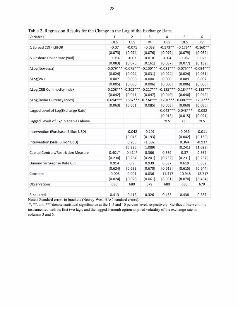
instrument FX interventions with the first two lags, as well as with the lagged option-implied 3-month volatility of the exchange rate. The use of lagged interventions as instruments is justified by the fact that once the Brazilian Central Bank decided to intervene, it did so for a long time, irrespective of the short term behavior of the exchange rate (as documented in Vervloet, 2010). For ease of interpretation of the coefficients, we multiply the variables that enter as log changes by 100, and measure the interest rate differential in percentage points. Our sample focuses on the period where Brazil was receiving sizable capital inflows and taking measures to discourage these flows. Our estimation sample begins in June 1, 2009 and ends in March 15, 2012 (when the controls/restrictions began to be gradually loosened). The exchange rate data is based on the PTAX rate published by the Brazilian Central Bank. That rate is based on an average of quotes from foreign exchange dealers in Brazil, and is the reference exchange rate typically used for future contracts (including offshore Non-Deliverable Forwards). Using that reference exchange rate also ensures that each daily data does not reflect capital control announcements made on that day (since the announcement of restrictions took place when the Brazilian market was closed). We use Bloomberg as the source for the remaining variables. Table 1 reports the results from this regression. The first column excludes the intervention variable. The coefficient on the interest rate differential is not significant (which may strike as surprising, but is in line with previous studies on Brazil, e.g. Vervloet, 2010 and Kohlscheen, 2011). The coefficient on the onshore dollar rate is not significant either, which may seem puzzling, but is consistent with the fact that periods where the onshore dollar rate was higher (for example, when controls temporarily succeeded in squeezing liquidity) were not accompanied by reduced appreciation pressures16.The point estimates suggest that a 1 percent increase in the local stock market or in commodity prices is associated with a 0.08 and 0.21 percent appreciation of the real, respectively. A one percent increase in the value of the dollar against advanced economy currencies are associated with a 0.70 depreciation of the real. The coefficient on the VIX is not statistically significant (but would become significant if the dollar currency index was dropped, which may be capturing changes in global risk aversion that would otherwise be explained by the VIX). The magnitudes are plausible and in line with previous estimates, and the coefficients in these variables remain comparable across all specifications in Table 1. The coefficient on the Capital Controls/Restriction Dummy is 0.4, and statistically significant

16The point estimates are compatible with the interpretation that increased onshore dollar rate attracts more funds, thereby appreciating the currency. This result was true before the controls (Vervloet 2010).

16

(suggesting that on average, each of the 12 measures considered appreciated the exchange rate by 0.4 percent).The dummy for the surprise cut in the policy rate is not statistically significant17. In Column 2 we add the central bank’s intervention as an additional variable. The estimates suggest that interventions had no effect on the exchange rate, neither when the central bank purchased dollars nor when it sold. In principle, the capital controls could have increased the traction of FX interventions (since they further segment the domestic and foreign financial markets, strengthening portfolio effects). But lack of an effect is consistent with the fact that the real steadily appreciated despite frequent and sizable interventions (Figure 6). There were only 6 instances where the central bank intervened by selling dollars in our sample, which makes it difficult to identify an effect. Sterilized sales became much more common after March 2012 (as shown in Figure 6). One possible explanation for why the central bank buying dollars does not affect the exchange rate involves the onshore dollar rate market. As explained before, and documented by Figure 2, the onshore dollar rate in Brazil runs above the equivalent rate in the US. When the Brazilian Central Bank conducts sterilized purchases of foreign exchange, the onshore dollar rate increases and large banks start bringing short term funds borrowed abroad to profit from the higher interest rate differential, without incurring in currency risk. The increase in the supply of foreign exchange provided by this dollar-interest-rate arbitrage tends to mitigate the effect of the sterilized purchases on the exchange rate. However, the reverse effect does not occur. When the Central Bank conducts sterilized sales of foreign exchange, thereby lowering the onshore dollar rate, this does not entice banks to borrow dollars in Brazil and invest them abroad, since the onshore dollar rate is still superior to its counterpart abroad. Columns 4-6 are analogous to Columns 1-3 but also include the lagged level of the log of the exchange rate, interest rate spread, onshore dollar rate, VIX, commodity prices and dollar index as controls. This specification allows the exchange rate to revert to a long-run level that will depend on the levels of these other explanatory variables (an error correction model). The results are fairly comparable to those in Columns 1-3. The coefficient on the interest rate differential becomes significant, but its magnitude remains very small (a 1 percent increase would appreciate the real by only 0.16 percent on impact). The coefficients on the lagged levels of the independent variables are not reported for the sake of conciseness. The coefficient on the lagged level of the log exchange rate is -0.04 and -0.05 in columns 4 and 5 (suggesting that in any given day, a one percent deviation from the long-run level is associated with a 0.04 and 0.05 percent correction towards that level, respectively). That coefficient is not statistically significant in column 6. 17 On the COPOM (Brazilian MPC) meeting of August 30, 2011, it was decided to revert the course of monetary policy. The basic rate, which had been climbing amid concerns of inflation acceleration, was unexpectedly cut by 50 bps, ushering in a long period of cuts that totaled 5.25 bps in a year.

17

In the regressions above we combined all the different capital controls and restrictions into a single dummy variable. One alternative is to code every capital control/restriction measure as a separate singleton dummy variable. We ran the same regressions from Table 1 replacing the single capital control/restriction variable by a full set of singleton dummies. The point estimates and standard errors for those dummies are reported in Table 2. The only dummies that are statistically significant with the “right” sign correspond to the initial capital control, the tax on the notional amount of derivatives and the tax on foreign borrowing up to 5 years, which depreciated the real by 1.2, 1.4 and 2.3 percent, respectively. None of the other dummies associated with restrictions are statistically significant, except for the tax on external borrowing up to 2 years, which is significant but suggests an appreciation of 1.1 percent (which has the “wrong” sign relative to what would be expected). An F-test for the sum of the coefficient on all the dummies related to capital controls and restrictions has a point estimate close to 3.5 percent which is not statistically significant.18 It is conceivable that some measures may have had a muted effect on impact, but could have had a larger effect in the aftermath, once the market got a better sense of their implications. Indeed Figure 6 seems to suggest the potential for breaks in trends following some of the measures. One way to gauge whether the breaks suggested in Figure 6 are driven by the controls/measures or global factors is to compare the behavior of the Brazilian real with that of other emerging market currencies around the time of those measures. While the Brazilian controls/measures could have some spillovers to other currencies, this effect should be second-order vis-à-vis the direct effect of changing global financial conditions. Figure 7 plots the evolution of the Australian dollar, Chilean and Colombian pesos, South African rand, and Turkish lira during this period. All of these currencies, except the Chilean peso, seem to reverse an appreciation trend following the initial capital control. All of these currencies, except the Australian dollar also seem to change their appreciation trends following the increase in the tax on fixed income flows. The trends in the rand and the Chilean peso also seem to “respond” to the restrictions on gross FX positions. The rand and the lira also revert appreciation trends following the tax on short-term external loans. And all of them tend to appreciate after the imposition of the tax on the notional amount of derivatives and the surprise rate cut. But the only currencies that seem to stabilize at a significantly more depreciated level towards the end of the sample are the real and the rand, both of which had domestic factors contributing to this outcome.

18 This limited response is also consistent with the behavior of the exchange rate at the time major restrictions were removed (which are not part of our estimation sample). For example, the real only appreciated 0.22% after the 6% tax on fixed income inflows was removed on June 2013, and depreciated 0.13% when the tax on the notional amount of derivatives was removed shortly afterwards.

18

In order to more formally test for an effect of the controls at different horizons, we ran similar regressions to the ones in Table 1 but spanning 2, 3 and 5-working day changes on the exchange rate and explanatory variables. If a measure becomes effective at time t, instead of dummies that capture the change from t-1 to t, these specifications will include dummies for the change from t-1 to t+1, t-1 to t+2, and t-1 to t+4. Table 4 reports the results for the two-day change. In the specifications where the capital control dummy is coded as 1 in the 12 dates in which measures are implemented, and 0 otherwise, that dummy looses its statistical significance over a two-day horizon (first row). When we run the regression using separate dummies for each measure, only the dummies for the initial 2 percent tax on portfolio inflows and the dummy for the tax on foreign borrowing with less than 5 year maturity remain statistically significant with a positive sign, with point estimates of about 1.6 and 2.5 percent, respectively. Some measures are significant but have a negative sign (e.g. the dummies related to the tax on foreign borrowing with maturities up to 1, and up to 2 years). The dummy on the surprise rate cut is now significant, and has a point estimate of about 2 percent. Table 5 is analogous to Table 4, but reports the results for a 3-day change in the exchange rate and explanatory variables. In the specifications with a single dummy coded as 1 in the 12 dates with restrictions, that dummy is significant in some specifications but not in others. In the specifications where it is significant, its point estimate is 0.46 and 0.47, which is similar to the point estimates for the one-day change in Table 2. Turning to the specification where each measure is coded by a separate dummy, only the dummy for the taxation of foreign borrowing with less than 5 year maturity remains significant, with a point estimate comparable to the one in Tables 2 and 3. The dummy on the surprise rate cut remains significant, and its point estimate ranges from 2 to 2.8. When we estimate the results for a 5-day change—which are not reported for the sake of conciseness—the dummy on the surprise rate cut remains significant. The only other dummy that is significant is the one related to the taxation of ADR issuance (but only in some specifications), with a point estimate of about 2.25 percent. Given the nature of the exchange rate process, the errors tend to increase over the horizon, and we should expect the effects to become less precisely estimated. To summarize, the results above do suggest a couple of measures had some success in depreciating the real. But even treating all of the estimated significant effects as permanent, their combined effect would only amount to about a 5 percent appreciation. While that is non-negligible, it sets an upper bound on what we can attribute to the combined effort of 12 measures. On balance, the effect on the exchange rate seems small relative to the effort that was placed in discouraging capital flows. We are still left in want of an explanation for why the real eventually settled at a more depreciated level, and did so only after the government had started easing its restrictions. In Figure 8 we plot the actual exchange rate as well as the fitted exchange rate implied by a regression of the log of the exchange rate on the log of the explanatory variables (excluding capital control/measure dummies and sterilized interventions). This regression is equivalent to

19

the co-integration relationship estimated in an error-correction model, and is estimated in different sub-samples, so we can compare the out-of-sample results with the actual exchange rate. There is a vast literature beginning with Meese and Rogoff (1981), recently reviewed in Engel (2013), that shows how difficult it is to forecast exchange rates. But the goal of this exercise is not to forecast exchange rates. Instead it is just to gauge whether the sustained depreciation of the real in 2012 can potentially be explained by the evolution of these explanatory variables. As expected, the fitted values closely track the exchange rate in-sample, but diverge from actual values out-of-sample. We present results when the estimation sample ends in December 30, 2010 (last tightening of controls on portfolio flows), in July 26, 2012 (tax on the notional amount of derivatives), and March 15, 2012 (beginning of easing of restrictions). In all cases, the fitted values are only systematically below the actual exchange rate beginning around the time of the surprise interest rate cut and start of the monetary policy easing cycle. This divergence becomes more pronounced in the period after March 2012, when the easing of restrictions begins, with the fitted values hovering at a level 5 to 10 percent more appreciated than the actual exchange rate. It is possible that a 6 percent tax failed to deter flows in an environment where the policy rate was 12.5 percent, but that same tax proved more of a deterrent in a lower interest rate environment (the policy rate was cut by 525bp over the easing cycle that begin with the October 2011 surprise cut). When estimating the effect of a given measure on the exchange rate, our dummy variable captured a snapshot at that particular time. It is possible that the very same measure would have had a larger effect if imposed in an environment with a lower policy rate.19 Market participants tend to attribute the eventual weakening of the real to a combination of investors becoming “fed-up” with the controls, lower interest rates, and weaker growth prospects. The focus of our analysis has been the effect of the controls/restrictions on the exchange rate. But they also had an effect through prudential considerations. For example, there has been a dramatic reduction in short-term external borrowing following the imposition of the 6 percent tax (as shown in Figure 4). In March 2011 short-term (less than one year) external borrowing amounted to US$ 6.5 billion. In April 2011, following the tax on short-term borrowing, that flow drops to only US$26 million. This maturity lengthening has improved the country’s resilience against external shocks. A full fledged assessment of the welfare implications of the controls would have to include the costs associated with them. If the “benefit” is small, but so are the costs, the policy could be

19 We test for breaks in the coefficients on the interest rate differential and FX intervention following different capital controls/restrictions, but do not find evidence of a significant break.

20

worthwhile. The controls did imply an increase in the cost of funding for Brazilian firms. The amount they were able to raise through equity financing was affected by the 2 percent tax foreigners had to pay to buy that equity. In the case of debt financing, the taxes could be avoided by borrowing abroad long-term. Given how flat the (dollar) yield curve was, borrowing long-term may have been a relatively small cost (which may well pay-off if the crisis were to deepen and global credit markets to dry). Small firms could not tap foreign markets directly, and their cost of funding may have been more affected by the controls. The taxes on derivative trades were fine-tuned so as to avoid incidence in the case of bona fide hedging by exporters (although taxing “speculators” can still hurt those firms by affecting the liquidity of those markets, as it seems to have happened since liquidity fell substantially). Some market analysts have attributed Brazil’s weak growth performance to a self-inflicted “sudden stop” (Volpon 2013) originating from the combination of economic policy deterioration and capital controls.

IV. CONCLUSION

Controls on capital inflows have gained renewed interest in the last years. From the theoretical point of view, many models have shown the desirability of some forms of prudential controls of capital inflows to enhance welfare in an environment of incomplete markets with pecuniary externalities (for a review, see Korinek 2011). From the policy perspective, the IMF, most notably, has changed the tone on capital controls (IMF 2012). The interest on practical experiences with controls on capital inflows increased substantially. Brazil provided the most cited example, because it has been experimenting with many different forms of controls on capital inflows. These controls were market-based in an open-economy with developed capital markets with low credit risk. Our results indicate that the controls were effective in the sense of creating distortions in the pricing of financial assets, i.e., making the domestic assets more expensive. That is, controls were effective in the sense of partially segmenting the Brazilian financial market from the international market. Controls had some limited success in containing the appreciation of the real when capital inflows were strong. But our most generous reading of the evidence, focusing only on the positive and statistically significant effects and treating those effects as permanent, amounts to less than 5 percent. This is a small effect in light of the several broad restrictions that were deployed over the course of two years and a half, suggesting capital controls are a relatively ineffective tool to manage the exchange rate. Capital controls may have also been a distraction from other policies that could have more effectively contained appreciation pressures (e.g. a rebalancing of the macro policy mix towards tighter fiscal policy so the inflation target could be met with lower interest rates). Given the weak state of the global economy together with the diminished interest that foreign investors have been devoting to Brazil recently, capital inflows have waned and most of the controls have been undone. Controls may have helped Brazil to avoid a bubble and perhaps

21

worse.20 However, given the very low domestic saving rate of the Brazilian economy (16%), constraining access to foreign financing likely contributed to the low investment and growth performance during that period.

20Even with the controls, the credit to GDP ratio more than doubled from 25% in 2003 to 50% by 2010.

22

References Auguste, Sebastian, Kathryn Domingues, Herman Kamil and Linda Tesar, 2002, “Cross-Border

Trading as a Mechanism for Capital Flight: ADRs and the Argentine Crisis,” NBER Working Paper No. 9343.

Baumann, Brittany, and Kevin Gallagher, 2012. “Navigating Capital Flows in Brazil and Chile”

Initiative for Policy Dialogue Working Paper. Benelli, Roberto, Alex Segura-Ubiergo and Chris Walker, 2011. “Brazil’s Experience Managing

Capital Inflows: The Role of Capital Flow Management Measures.” IMF Selected Issues Paper.

Cardenas, Mauricio, and Felipe Barrera, 1997, “On the Effectiviness of Capital Controls: The

Experience of Colombia during the 1990s,” Journal of Development Economics, v54(1), pp. 27-57.

Cardoso, Eliana and Ilan Goldfajn, 1998, “Capital Flows to Brazil: The Endogeneity of Capital

Controls,” IMF Staff Papers, Vol. 45(1), pp. 161–202. Carvalho, Bernardo S. de M., and Márcio G. P. Garcia, 2008, “Ineffective Controls on Capital

Inflows under Sophisticated Financial Markets: Brazil in the Nineties,” in S. Edwards and M. Garcia, eds., Financial Markets Volatility and Performance in Emerging Markets (Cambridge, Massachusetts: National Bureau of Economic Research).

de Gregório, José, Sebastian Edwards, and Rodrigo Valdés, 2000, “Controls on Capital Inflows:

Do They Work?”Journal of Development Economics, v. 63(1), pp. 59-83 Didier, Tatiana and Márcio Garcia, 2003, “Very High Interest Rates in Brazil and the Cousin

Risks: Brazil During the Real Plan”, Pesquisa e Planejamento Econômico, v.33, n.2, p.253-297.

Edwards, Sebastian, and Roberto Rigobon, 2009, “Capital Controls on Inflows, Exchange Rate

Volatility and External Vulnerability,” Journal of International Economics, v.78(2), pp. 256-67.

Edwards, Sebastian, 1999, “How Effective Are Capital Controls?” Journal of Economic

Perspectives, v.13 (4), pp. 65-84. Engel, Charles, 2013, “Exchange Rates and Interest Parity”, NBER Discussion Paper #19336.

23

Forbes, Kristin, 2007, “One cost of the Chilean capital controls: increased financial constraints for

smaller traded firms,” Journal of International Economics, Vol 71(2), pp. 294-323. Forbes, K., M. Fratzscher, T. Kostka, and R. Straub, 2012, Bubble Thy Neighbor: Portfolio Effects

and Externalities from Capital Controls. NBER Working Paper No. 18052, May. IMF, 2012, “The Liberalization and Management of Capital Flows - An Institutional View,”

available at http://www.imf.org/external/np/pp/eng/2012/111412.pdf Jeanne, Olivier, Arvind Subramanian and John Williamson, 2012, Who Needs to Open the Capital

Account? Washington DC: Peterson Institute for International Economics. Jinjarak, Yothin, Ilan Noy, and Huanhuan Zheng, 2013, “Capital controls in Brazil - Stemming a

tide with a signal?” Journal of Banking & Finance, Vol. 37, pp. 2938-2952. Klein, Michael, 2012, “Capital controls: Gates versus Walls” NBER Working Paper No. 18526. Kohlscheen, Emanuel, 2011, “The impact of monetary policy on the exchange rate: a higher

frequency exchange rate puzzle in emerging economies?” Banco Central do Brasil Working Paper No. 259.

Korinek, Anton, 2011, “The Economics of Prudential Capital Controls: A Research Agenda”, IMF

Economic Review, Vol. 59, No. 3, pp. 523-561. Meese, Richard, and Kenneth Rogoff, 1983. “Empirical Exchange Rate Models of the Seventies.”

Journal of International Economics, Vol. 14, pp. 3-24. Magud, Nicolas, Carmen Reinhart and Kenneth Rogoff, 2011, “Capital Controls: Myth and Reality

– A Portfolio Balance Approach,” NBER Working Paper No. 16805. Ostry, Jonathan D., Atish Ghosh, Karl Habermeier, Marcos Chamon, Mahvash Qureshi, and

Dennis Reinhart, 2010, “Capital Inflows: The Role of Controls,” IMF Staff Position Note No. 2010/04.

Ostry, Jonathan D., Atish Ghosh, Marcos Chamon, and Mahvash Qureshi, 2012, “Tools for

managing financial-stability risks from capital inflows,” Journal of International Economics, Vol. 88(2), pp. 407-421.

24

Pereira da Silva, Luiz and Ricardo Harris, 2012, “Sailing through the Global Financial Storm:

Brazil’s Recent Experience with Monetary and Macroprudential Policies to Lean against the Financial Cycle and Deal with Systemic Risks,” Brazilian Central Bank Working Paper Series, No. 290, August.

Ranciere, Romain, Aaron Tornell, and Athanasios Vamvakidis, 2010, “Currency mismatch,

systemic risk and growth in emerging Europe.” Economic Policy, Vol. 25, pp. 597-658. Rey, Helene, 2013, “Dilemma not Trilemma: The Global Financial Cycle and Monetary Policy

Independence”, mimeo, Kansas FED Jackson Hole Conference. Ventura, André and Márcio Garcia, 2012,“Mercados Futuros e À Vista de Câmbio no Brasil: O

Rabo Abana o Cachorro”, Revista Brasileira de Economia, Vol. 66, No. 1, Jan-Mar, pp. 21-48.

Vervloet, W. (2010). Efeitos de intervenções esterilizadas do Banco Central do Brasil sobre a taxa

de câmbio. PUC-Rio M.Sc. Dissertation. Mimeo. Volpon, Tony (2013). “Brazil: Self-inflicted “sudden stop”” Nomura Research Report.

25

Appendix A1. Regression Results for Volume of Capital Flows. In this appendix we more formally assess the impact of the capital controls/restrictions on the volume of capital flows through regressions. Data on the volume of flows is available at a monthly frequency. We consider a sample covering 2007M1-2012M12. Given the smaller number of observations (due to the monthly frequency), we only code dummies for: the initial tax on portfolio debt and equity flows (2009M10), the increase the tax on fixed income flows (2010M10), the taxation of short-term external loans (2011M3), the beginning of interest rate easing cycle (2011M9), and the beginning of the removal of restrictions (coded as 2011M12 for portfolio equity, 2012M3 for all other flows).We also code a dummy for the Global Financial Crisis, which equals one during 2008M9-2009M3, in order to capture the sharp reversal in flows during that period. The volume of capital flows is not an I(1) variable, and as a result, we run regressions on the level of flows (millions of current US$) and use step dummies for the capital control/restriction variables (i.e. the dummy is coded as 0 prior to the month a measure is adopted; 1 from that month onwards). Table A1 presents the regression results. Column 1 considers portfolio debt flows. None of the dummies related to capital controls/restrictions is significant. The dummy for the interest rate easing cycle is significant, indicating a 1 billion USD dollar drop in monthly flows from that point onward. As expected, the dummy for the Global Financial Crisis is significant and points to a large drop in flows during that period. The coefficient on the lagged dependent variable points to little or no persistence in the flow data. Column 2 adds the explanatory variables used in the exchange rate regressions as well as the Brazilian real exchange rate. These explanatory variables enter in levels, and are based on their period-average during the corresponding month. All have statistically significant coefficients, although some variables have the opposite sign expected (e.g. a negative coefficient on the interest rate differential). Columns 3 and 4 are analogous to Columns 1 and 2 but focus on portfolio equity flows. As in the case of portfolio debt flows, none of the dummies related to the capital controls/restrictions seem to have affected portfolio equity flows. Columns 5 and 6 turn to FDI. The dummy on the increase in the tax on fixed income flows is significant and point to a sharp increase in FDI in both specifications, while the taxation of short-term external loans is significant only in Column 6, pointing to a contraction of FDI following that measure. While it is possible that the tax on fixed income flows led to a shift towards FDI, and that the tax on short-term external loans somehow impacted FDI flows, the results may well be spurious. As indicated in the main text of the paper, by all accounts it is very difficult to disguise portfolio flows as FDI, and if some relabeling took place, it likely only did so at the margins. Finally columns 7 and 8 turn to other flows (which include bank loans, inter-bank transactions, trade credit, among others). The results in column 7 suggest an expansion on these flows following the taxation of short-term external loans, a contraction following the beginning of the interest rate easing cycle, and an expansion

26

following the beginning of removal of capital controls/restrictions. Column 8 also points to a contraction in flows following the initial control, while the coefficient on the removal of restrictions is no longer statistically significant. There is some margin for substitution between portfolio flows and some types of other flows, e.g. firms borrowing directly abroad following the taxation of fixed income flows. In that regard, it is surprising that other flows increase following the tax on borrowing short-term abroad (although one could avoid that tax simply by borrowing long-term, which was relatively cheap given the flat dollar yield curve). But overall, the results on the volume of flows are quite mixed, consistent Figure 1, which does not suggest any clear pattern in the aftermath of these measures.

27

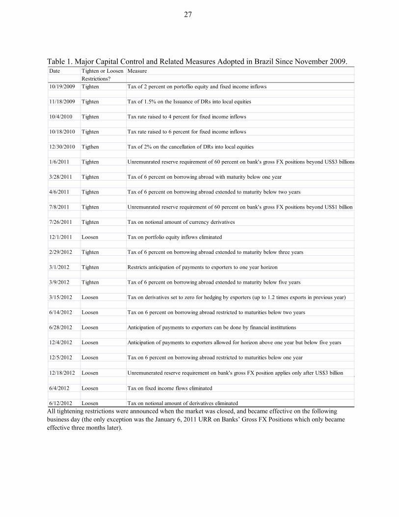
Table 1. Major Capital Control and Related Measures Adopted in Brazil Since November 2009.

All tightening restrictions were announced when the market was closed, and became effective on the following business day (the only exception was the January 6, 2011 URR on Banks’ Gross FX Positions which only became effective three months later).

Date Tighten or Loosen Measure

Restrictions?

10/19/2009 Tighten Tax of 2 percent on portoflio equity and fixed income inflows

11/18/2009 Tighten Tax of 1.5% on the Issuance of DRs into local equities

10/4/2010 Tighten Tax rate raised to 4 percent for fixed income inflows

10/18/2010 Tighten Tax rate raised to 6 percent for fixed income inflows

12/30/2010 Tigthen Tax of 2% on the cancellation of DRs into local equities

1/6/2011 Tighten Unremunrated reserve requirement of 60 percent on bank's gross FX positions beyond US$3 billions

3/28/2011 Tighten Tax of 6 percent on borrowing abroad with maturity below one year

4/6/2011 Tighten Tax of 6 percent on borrowing abroad extended to maturity below two years

7/8/2011 Tighten Unremunrated reserve requirement of 60 percent on bank's gross FX positions beyond US$1 billion

7/26/2011 Tighten Tax on notional amount of currency derivatives

12/1/2011 Loosen Tax on portfolio equity inflows eliminated

2/29/2012 Tighten Tax of 6 percent on borrowing abroad extended to maturity below three years

3/1/2012 Tighten Restricts anticipation of payments to exporters to one year horizon

3/9/2012 Tighten Tax of 6 percent on borrowing abroad extended to maturity below five years

3/15/2012 Loosen Tax on derivatives set to zero for hedging by exporters (up to 1.2 times exports in previous year)

6/14/2012 Loosen Tax on 6 percent on borrowing abroad restricted to maturities below two years

6/28/2012 Loosen Anticipation of payments to exporters can be done by financial instittutions

12/4/2012 Loosen Anticipation of payments to exporters allowed for horizon above one year but below five years

12/5/2012 Loosen Tax on 6 percent on borrowing abroad restricted to maturities below one year

12/18/2012 Loosen Unremunerated reserve requirement on bank's gross FX position applies only after US$3 billion

6/4/2012 Loosen Tax on fixed income flows eliminated

6/12/2012 Loosen Tax on notional amount of derivatives eliminated

28

Table 2. Regression Results for the Change in the Log of the Exchange Rate.

Notes: Standard errors in brackets (Newey-West HAC standard errors). *, **, and *** denote statistical significance at the 1, 5 and 10 percent level, respectively. Sterilized Interventions instrumented with its first two lags, and the lagged 3-month option-implied volatility of the exchange rate in columns 3 and 6.

Variables 1 2 3 4 5 6

OLS OLS IV OLS OLS IV

Spread CDI - LIBOR -0.07 -0.071 -0.058 -0.173** -0.176** -0.160**

[0.073] [0.074] [0.076] [0.079] [0.079] [0.082]

Onshore Dollar Rate (90d) -0.054 -0.07 0.018 -0.04 -0.067 0.025

[0.083] [0.075] [0.161] [0.087] [0.077] [0.162]

Log(Ibovespa) -0.079*** -0.075*** -0.100*** -0.081*** -0.075*** -0.094***

[0.024] [0.024] [0.031] [0.024] [0.024] [0.031]

Log(Vix) 0.007 0.008 0.004 0.008 0.009 0.007

[0.005] [0.006] [0.006] [0.006] [0.006] [0.006]

Log(CRB Commodity Index) -0.208*** -0.202*** -0.217*** -0.185*** -0.184*** -0.182***

[0.042] [0.041] [0.047] [0.040] [0.040] [0.042]

Log(Dollar Currency Index) 0.694*** 0.682*** 0.734*** 0.701*** 0.686*** 0.731***

[0.063] [0.061] [0.085] [0.063] [0.060] [0.085]

Lagged Level of Log(Exchange Rate) -0.043*** -0.048*** -0.032

[0.015] [0.015] [0.021]

Lagged Levels of Exp. Variables Above YES YES YES

Intervention (Purchase, Billion USD) -0.042 -0.101 -0.056 -0.011

[0.043] [0.193] [0.042] [0.159]

Intervention (Sale, Billion USD) 0.285 -1.382 0.364 -0.937

[0.236] [1.089] [0.241] [1.093]

Capital Controls/Restriction Measure 0.401* 0.414* 0.366 0.369 0.37 0.367

[0.234] [0.234] [0.241] [0.232] [0.231] [0.237]

Dummy for Surprise Rate Cut 0.914 0.9 0.939 0.637 0.619 0.652

[0.624] [0.623] [0.670] [0.618] [0.615] [0.644]

Constant -0.003 0.001 0.036 -11.417 -10.948 -12.717

[0.024] [0.028] [0.061] [8.031] [8.070] [8.434]

Observations 680 680 679 680 680 679

R-squared 0.413 0.416 0.326 0.433 0.438 0.387

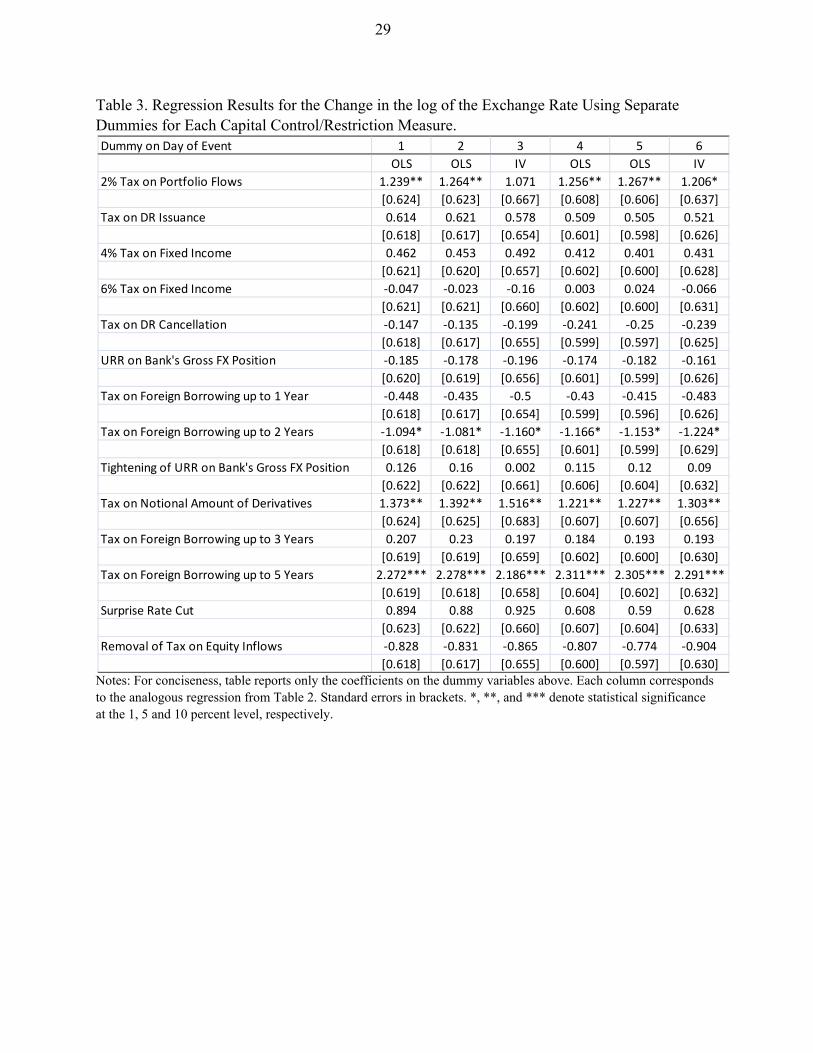
29

Table 3. Regression Results for the Change in the log of the Exchange Rate Using Separate Dummies for Each Capital Control/Restriction Measure.

Notes: For conciseness, table reports only the coefficients on the dummy variables above. Each column corresponds to the analogous regression from Table 2. Standard errors in brackets. *, **, and *** denote statistical significance at the 1, 5 and 10 percent level, respectively.

Dummy on Day of Event 1 2 3 4 5 6

OLS OLS IV OLS OLS IV

2% Tax on Portfolio Flows 1.239** 1.264** 1.071 1.256** 1.267** 1.206*

[0.624] [0.623] [0.667] [0.608] [0.606] [0.637]

Tax on DR Issuance 0.614 0.621 0.578 0.509 0.505 0.521

[0.618] [0.617] [0.654] [0.601] [0.598] [0.626]

4% Tax on Fixed Income 0.462 0.453 0.492 0.412 0.401 0.431

[0.621] [0.620] [0.657] [0.602] [0.600] [0.628]

6% Tax on Fixed Income -0.047 -0.023 -0.16 0.003 0.024 -0.066

[0.621] [0.621] [0.660] [0.602] [0.600] [0.631]

Tax on DR Cancellation -0.147 -0.135 -0.199 -0.241 -0.25 -0.239

[0.618] [0.617] [0.655] [0.599] [0.597] [0.625]

URR on Bank's Gross FX Position -0.185 -0.178 -0.196 -0.174 -0.182 -0.161

[0.620] [0.619] [0.656] [0.601] [0.599] [0.626]

Tax on Foreign Borrowing up to 1 Year -0.448 -0.435 -0.5 -0.43 -0.415 -0.483

[0.618] [0.617] [0.654] [0.599] [0.596] [0.626]

Tax on Foreign Borrowing up to 2 Years -1.094* -1.081* -1.160* -1.166* -1.153* -1.224*

[0.618] [0.618] [0.655] [0.601] [0.599] [0.629]

Tightening of URR on Bank's Gross FX Position 0.126 0.16 0.002 0.115 0.12 0.09

[0.622] [0.622] [0.661] [0.606] [0.604] [0.632]

Tax on Notional Amount of Derivatives 1.373** 1.392** 1.516** 1.221** 1.227** 1.303**

[0.624] [0.625] [0.683] [0.607] [0.607] [0.656]

Tax on Foreign Borrowing up to 3 Years 0.207 0.23 0.197 0.184 0.193 0.193

[0.619] [0.619] [0.659] [0.602] [0.600] [0.630]

Tax on Foreign Borrowing up to 5 Years 2.272*** 2.278*** 2.186*** 2.311*** 2.305*** 2.291***

[0.619] [0.618] [0.658] [0.604] [0.602] [0.632]

Surprise Rate Cut 0.894 0.88 0.925 0.608 0.59 0.628

[0.623] [0.622] [0.660] [0.607] [0.604] [0.633]

Removal of Tax on Equity Inflows -0.828 -0.831 -0.865 -0.807 -0.774 -0.904

[0.618] [0.617] [0.655] [0.600] [0.597] [0.630]

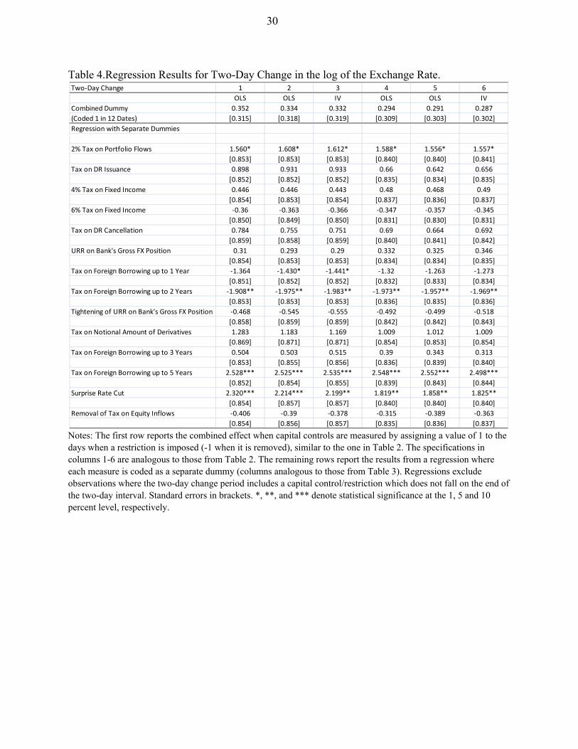
30

Table 4.Regression Results for Two-Day Change in the log of the Exchange Rate.

Notes: The first row reports the combined effect when capital controls are measured by assigning a value of 1 to the days when a restriction is imposed (-1 when it is removed), similar to the one in Table 2. The specifications in columns 1-6 are analogous to those from Table 2. The remaining rows report the results from a regression where each measure is coded as a separate dummy (columns analogous to those from Table 3). Regressions exclude observations where the two-day change period includes a capital control/restriction which does not fall on the end of the two-day interval. Standard errors in brackets. *, **, and *** denote statistical significance at the 1, 5 and 10 percent level, respectively.

Two-Day Change 1 2 3 4 5 6

OLS OLS IV OLS OLS IV

Combined Dummy 0.352 0.334 0.332 0.294 0.291 0.287

(Coded 1 in 12 Dates) [0.315] [0.318] [0.319] [0.309] [0.303] [0.302]

Regression with Separate Dummies

2% Tax on Portfolio Flows 1.560* 1.608* 1.612* 1.588* 1.556* 1.557*

[0.853] [0.853] [0.853] [0.840] [0.840] [0.841]

Tax on DR Issuance 0.898 0.931 0.933 0.66 0.642 0.656

[0.852] [0.852] [0.852] [0.835] [0.834] [0.835]

4% Tax on Fixed Income 0.446 0.446 0.443 0.48 0.468 0.49

[0.854] [0.853] [0.854] [0.837] [0.836] [0.837]

6% Tax on Fixed Income -0.36 -0.363 -0.366 -0.347 -0.357 -0.345

[0.850] [0.849] [0.850] [0.831] [0.830] [0.831]

Tax on DR Cancellation 0.784 0.755 0.751 0.69 0.664 0.692

[0.859] [0.858] [0.859] [0.840] [0.841] [0.842]

URR on Bank's Gross FX Position 0.31 0.293 0.29 0.332 0.325 0.346

[0.854] [0.853] [0.853] [0.834] [0.834] [0.835]

Tax on Foreign Borrowing up to 1 Year -1.364 -1.430* -1.441* -1.32 -1.263 -1.273

[0.851] [0.852] [0.852] [0.832] [0.833] [0.834]

Tax on Foreign Borrowing up to 2 Years -1.908** -1.975** -1.983** -1.973** -1.957** -1.969**

[0.853] [0.853] [0.853] [0.836] [0.835] [0.836]

Tightening of URR on Bank's Gross FX Position -0.468 -0.545 -0.555 -0.492 -0.499 -0.518

[0.858] [0.859] [0.859] [0.842] [0.842] [0.843]

Tax on Notional Amount of Derivatives 1.283 1.183 1.169 1.009 1.012 1.009

[0.869] [0.871] [0.871] [0.854] [0.853] [0.854]

Tax on Foreign Borrowing up to 3 Years 0.504 0.503 0.515 0.39 0.343 0.313

[0.853] [0.855] [0.856] [0.836] [0.839] [0.840]

Tax on Foreign Borrowing up to 5 Years 2.528*** 2.525*** 2.535*** 2.548*** 2.552*** 2.498***

[0.852] [0.854] [0.855] [0.839] [0.843] [0.844]

Surprise Rate Cut 2.320*** 2.214*** 2.199** 1.819** 1.858** 1.825**

[0.854] [0.857] [0.857] [0.840] [0.840] [0.840]

Removal of Tax on Equity Inflows -0.406 -0.39 -0.378 -0.315 -0.389 -0.363

[0.854] [0.856] [0.857] [0.835] [0.836] [0.837]

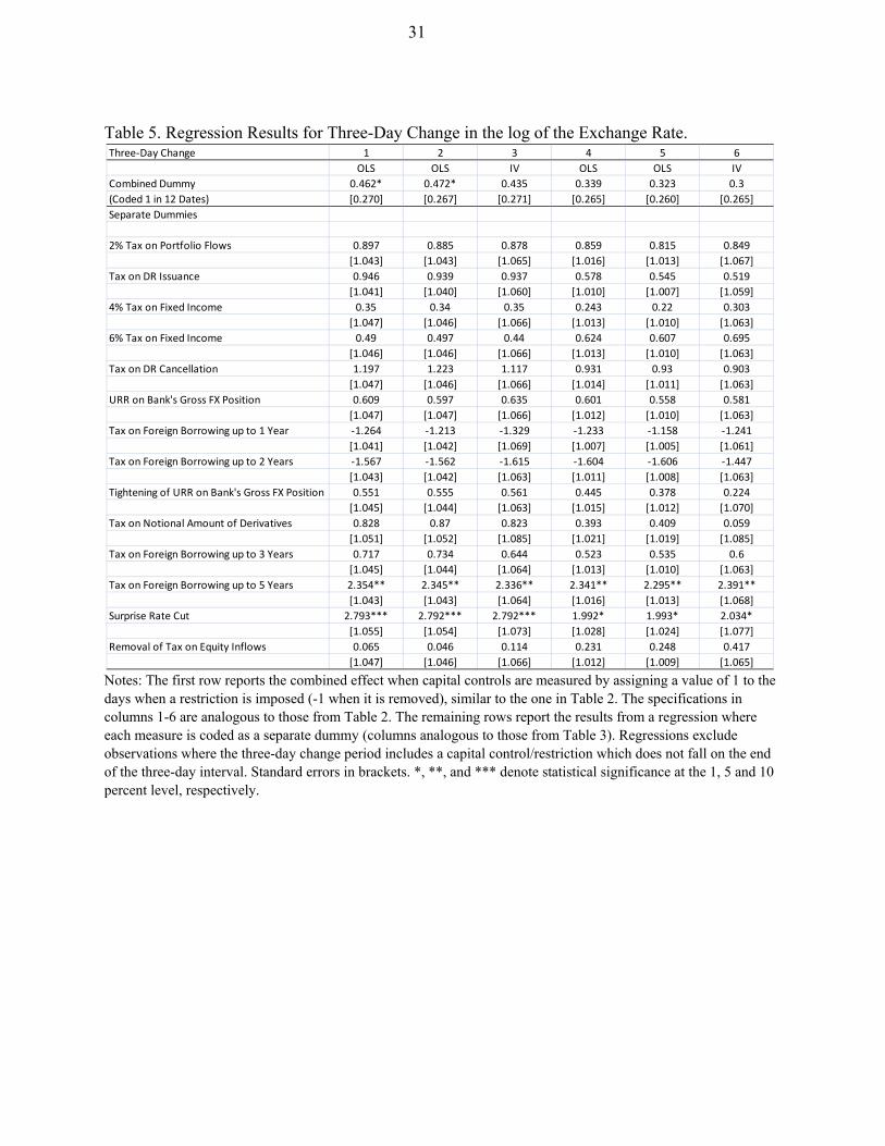
31

Table 5. Regression Results for Three-Day Change in the log of the Exchange Rate.

Notes: The first row reports the combined effect when capital controls are measured by assigning a value of 1 to the days when a restriction is imposed (-1 when it is removed), similar to the one in Table 2. The specifications in columns 1-6 are analogous to those from Table 2. The remaining rows report the results from a regression where each measure is coded as a separate dummy (columns analogous to those from Table 3). Regressions exclude observations where the three-day change period includes a capital control/restriction which does not fall on the end of the three-day interval. Standard errors in brackets. *, **, and *** denote statistical significance at the 1, 5 and 10 percent level, respectively.

Three-Day Change 1 2 3 4 5 6

OLS OLS IV OLS OLS IV

Combined Dummy 0.462* 0.472* 0.435 0.339 0.323 0.3

(Coded 1 in 12 Dates) [0.270] [0.267] [0.271] [0.265] [0.260] [0.265]

Separate Dummies

2% Tax on Portfolio Flows 0.897 0.885 0.878 0.859 0.815 0.849

[1.043] [1.043] [1.065] [1.016] [1.013] [1.067]

Tax on DR Issuance 0.946 0.939 0.937 0.578 0.545 0.519

[1.041] [1.040] [1.060] [1.010] [1.007] [1.059]

4% Tax on Fixed Income 0.35 0.34 0.35 0.243 0.22 0.303

[1.047] [1.046] [1.066] [1.013] [1.010] [1.063]

6% Tax on Fixed Income 0.49 0.497 0.44 0.624 0.607 0.695

[1.046] [1.046] [1.066] [1.013] [1.010] [1.063]

Tax on DR Cancellation 1.197 1.223 1.117 0.931 0.93 0.903

[1.047] [1.046] [1.066] [1.014] [1.011] [1.063]

URR on Bank's Gross FX Position 0.609 0.597 0.635 0.601 0.558 0.581

[1.047] [1.047] [1.066] [1.012] [1.010] [1.063]

Tax on Foreign Borrowing up to 1 Year -1.264 -1.213 -1.329 -1.233 -1.158 -1.241

[1.041] [1.042] [1.069] [1.007] [1.005] [1.061]

Tax on Foreign Borrowing up to 2 Years -1.567 -1.562 -1.615 -1.604 -1.606 -1.447

[1.043] [1.042] [1.063] [1.011] [1.008] [1.063]

Tightening of URR on Bank's Gross FX Position 0.551 0.555 0.561 0.445 0.378 0.224

[1.045] [1.044] [1.063] [1.015] [1.012] [1.070]

Tax on Notional Amount of Derivatives 0.828 0.87 0.823 0.393 0.409 0.059

[1.051] [1.052] [1.085] [1.021] [1.019] [1.085]

Tax on Foreign Borrowing up to 3 Years 0.717 0.734 0.644 0.523 0.535 0.6

[1.045] [1.044] [1.064] [1.013] [1.010] [1.063]

Tax on Foreign Borrowing up to 5 Years 2.354** 2.345** 2.336** 2.341** 2.295** 2.391**

[1.043] [1.043] [1.064] [1.016] [1.013] [1.068]

Surprise Rate Cut 2.793*** 2.792*** 2.792*** 1.992* 1.993* 2.034*

[1.055] [1.054] [1.073] [1.028] [1.024] [1.077]

Removal of Tax on Equity Inflows 0.065 0.046 0.114 0.231 0.248 0.417

[1.047] [1.046] [1.066] [1.012] [1.009] [1.065]

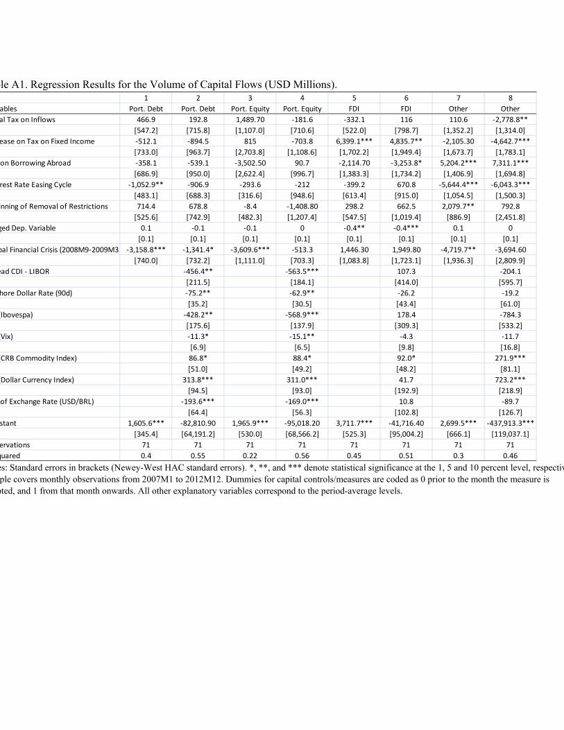
ble A1. Regression Results for the Volume of Capital Flows (USD Millions).

es: Standard errors in brackets (Newey-West HAC standard errors). *, **, and *** denote statistical significance at the 1, 5 and 10 percent level, respectivple covers monthly observations from 2007M1 to 2012M12. Dummies for capital controls/measures are coded as 0 prior to the month the measure is

pted, and 1 from that month onwards. All other explanatory variables correspond to the period-average levels.

1 2 3 4 5 6 7 8

ables Port. Debt Port. Debt Port. Equity Port. Equity FDI FDI Other Other

al Tax on Inflows 466.9 192.8 1,489.70 -181.6 -332.1 116 110.6 -2,778.8**

[547.2] [715.8] [1,107.0] [710.6] [522.0] [798.7] [1,352.2] [1,314.0]

ease on Tax on Fixed Income -512.1 -894.5 815 -703.8 6,399.1*** 4,835.7** -2,105.30 -4,642.7***

[733.0] [963.7] [2,703.8] [1,108.6] [1,702.2] [1,949.4] [1,673.7] [1,783.1]

on Borrowing Abroad -358.1 -539.1 -3,502.50 90.7 -2,114.70 -3,253.8* 5,204.2*** 7,311.1***

[686.9] [950.0] [2,622.4] [996.7] [1,383.3] [1,734.2] [1,406.9] [1,694.8]

rest Rate Easing Cycle -1,052.9** -906.9 -293.6 -212 -399.2 670.8 -5,644.4*** -6,043.3***

[483.1] [688.3] [316.6] [948.6] [613.4] [915.0] [1,054.5] [1,500.3]

inning of Removal of Restrictions 714.4 678.8 -8.4 -1,408.80 298.2 662.5 2,079.7** 792.8

[525.6] [742.9] [482.3] [1,207.4] [547.5] [1,019.4] [886.9] [2,451.8]

ged Dep. Variable 0.1 -0.1 -0.1 0 -0.4** -0.4*** 0.1 0

[0.1] [0.1] [0.1] [0.1] [0.1] [0.1] [0.1] [0.1]

bal Financial Crisis (2008M9-2009M3) -3,158.8*** -1,341.4* -3,609.6*** -513.3 1,446.30 1,949.80 -4,719.7** -3,694.60

[740.0] [732.2] [1,111.0] [703.3] [1,083.8] [1,723.1] [1,936.3] [2,809.9]

ead CDI - LIBOR -456.4** -563.5*** 107.3 -204.1

[211.5] [184.1] [414.0] [595.7]

hore Dollar Rate (90d) -75.2** -62.9** -26.2 -19.2

[35.2] [30.5] [43.4] [61.0]

(Ibovespa) -428.2** -568.9*** 178.4 -784.3

[175.6] [137.9] [309.3] [533.2]

(Vix) -11.3* -15.1** -4.3 -11.7

[6.9] [6.5] [9.8] [16.8]

(CRB Commodity Index) 86.8* 88.4* 92.0* 271.9***

[51.0] [49.2] [48.2] [81.1]

(Dollar Currency Index) 313.8*** 311.0*** 41.7 723.2***

[94.5] [93.0] [192.9] [218.9]

of Exchange Rate (USD/BRL) -193.6*** -169.0*** 10.8 -89.7

[64.4] [56.3] [102.8] [126.7]

stant 1,605.6*** -82,810.90 1,965.9*** -95,018.20 3,711.7*** -41,716.40 2,699.5*** -437,913.3***

[345.4] [64,191.2] [530.0] [68,566.2] [525.3] [95,004.2] [666.1] [119,037.1]

ervations 71 71 71 71 71 71 71 71

quared 0.4 0.55 0.22 0.56 0.45 0.51 0.3 0.46

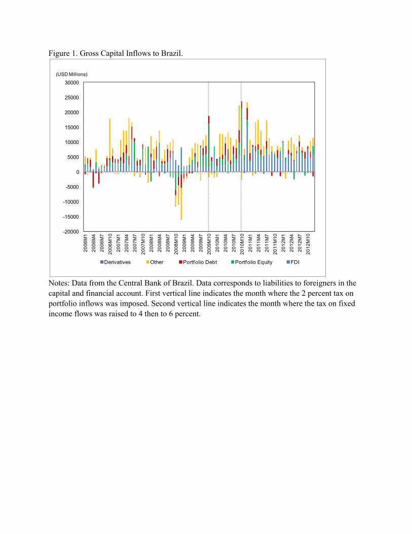
Figure 1. Gross Capital Inflows to Brazil.

Notes: Data from the Central Bank of Brazil. Data corresponds to liabilities to foreigners in the capital and financial account. First vertical line indicates the month where the 2 percent tax on portfolio inflows was imposed. Second vertical line indicates the month where the tax on fixed income flows was raised to 4 then to 6 percent.

-20000

-15000

-10000

-5000

0

5000

10000

15000

20000

25000

300002

00

6M

1

20

06

M4

20

06

M7

20

06

M1

0

20

07

M1

20

07

M4

20

07

M7

20

07

M1

0

20

08

M1

20

08

M4

20

08

M7

20

08

M1

0

20

09

M1

20

09

M4

20

09

M7

20

09

M1

0

20

10

M1

20

10

M4

20

10

M7

20

10

M1

0

20

11

M1

20

11

M4

20

11

M7

20

11

M1

0

20

12

M1

20

12

M4

20

12

M7

20

12

M1

0

(USD Millions)

Derivatives Other Portfolio Debt Portfolio Equity FDI

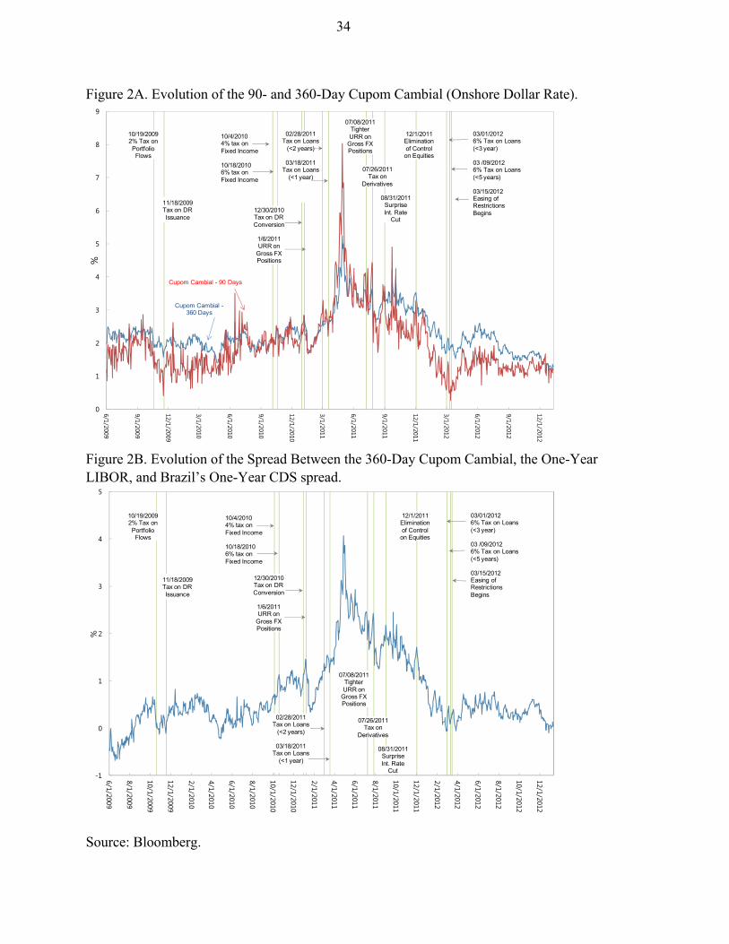
34

Figure 2A. Evolution of the 90- and 360-Day Cupom Cambial (Onshore Dollar Rate).

Figure 2B. Evolution of the Spread Between the 360-Day Cupom Cambial, the One-Year LIBOR, and Brazil’s One-Year CDS spread.

Source: Bloomberg.

0

1

2

3

4

5

6

7

8

9

6/1/2009

9/1/2009

12/1/2009

3/1/2010

6/1/2010

9/1/2010

12/1/2010

3/1/2011

6/1/2011

9/1/2011

12/1/2011

3/1/2012

6/1/2012

9/1/2012

12/1/2012

%

Cupom Cambial - 90 Days

Cupom Cambial -360 Days

10/19/20092% Tax on Portfolio Flows

11/18/2009Tax on DR Issuance

12/1/2011Eliminationof Control on Equities

03/01/20126% Tax on Loans(<3 year)

03 /09/20126% Tax on Loans(<5 years)

03/15/2012Easing of Restrictions Begins

07/08/2011Tighter URR on

Gross FX Positions

10/4/20104% tax on Fixed Income

10/18/20106% tax onFixed Income

02/28/2011Tax on Loans

(<2 years)

03/18/2011Tax on Loans

(<1 year)

12/30/2010Tax on DR Conversion

1/6/2011URR on

Gross FXPositions

07/26/2011Tax on

Derivatives

08/31/2011SurpriseInt. Rate

Cut

0

10

20

30

40

50

60

70

80

90

100

-1

0

1

2

3

4

5

6/1/2009

8/1/2009

10/1/2009

12/1/2009

2/1/2010

4/1/2010

6/1/2010

8/1/2010

10/1/2010

12/1/2010

2/1/2011

4/1/2011

6/1/2011

8/1/2011

10/1/2011

12/1/2011

2/1/2012

4/1/2012

6/1/2012

8/1/2012

10/1/2012

12/1/2012

%

10/19/20092% Tax on Portfolio Flows

11/18/2009Tax on DR Issuance

12/1/2011Eliminationof Control on Equities

03/01/20126% Tax on Loans(<3 year)

03 /09/20126% Tax on Loans(<5 years)

03/15/2012Easing of Restrictions Begins

07/08/2011Tighter URR on

Gross FX Positions

10/4/20104% tax on Fixed Income

10/18/20106% tax onFixed Income

02/28/2011Tax on Loans

(<2 years)

03/18/2011Tax on Loans

(<1 year)

12/30/2010Tax on DR Conversion

1/6/2011URR on

Gross FXPositions

07/26/2011Tax on

Derivatives

08/31/2011SurpriseInt. Rate

Cut

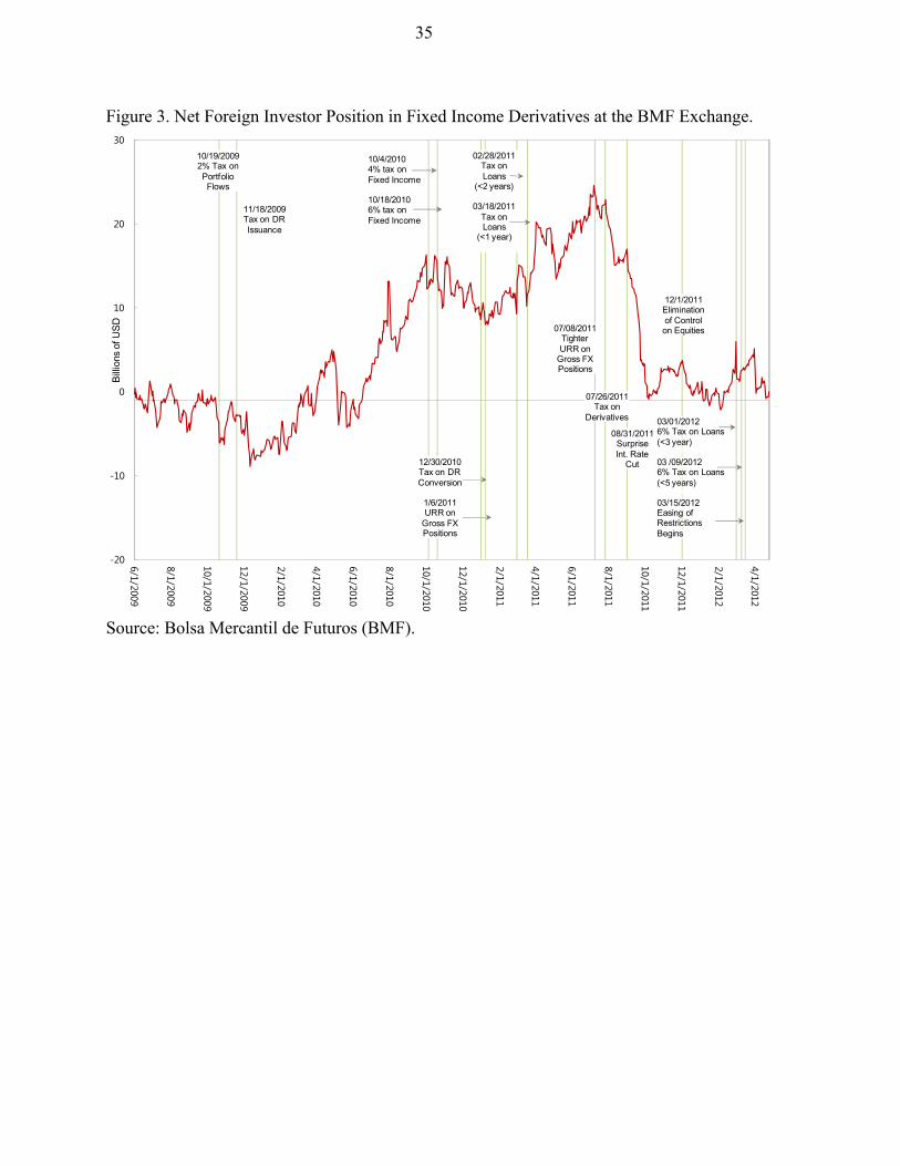
35

Figure 3. Net Foreign Investor Position in Fixed Income Derivatives at the BMF Exchange.

Source: Bolsa Mercantil de Futuros (BMF).

-100

-90

-80

-70

-60

-50

-40

-30

-20

-10

0

-20

-10

0

10

20

30

6/1/2009

8/1/2009

10/1/2009

12/1/2009

2/1/2010

4/1/2010

6/1/2010

8/1/2010

10/1/2010

12/1/2010

2/1/2011

4/1/2011

6/1/2011

8/1/2011

10/1/2011

12/1/2011

2/1/2012

4/1/2012

Bill

ions

of U

SD

10/19/20092% Tax on Portfolio Flows

11/18/2009Tax on DR Issuance

12/1/2011Eliminationof Control on Equities07/08/2011

Tighter URR on

Gross FX Positions

10/4/20104% tax on Fixed Income

10/18/20106% tax onFixed Income

02/28/2011Tax on Loans

(<2 years)

03/18/2011Tax on Loans

(<1 year)

12/30/2010Tax on DR Conversion

1/6/2011URR on

Gross FXPositions

07/26/2011Tax on

Derivatives 03/01/20126% Tax on Loans(<3 year)

03 /09/20126% Tax on Loans(<5 years)

03/15/2012Easing of Restrictions Begins

08/31/2011SurpriseInt. Rate

Cut

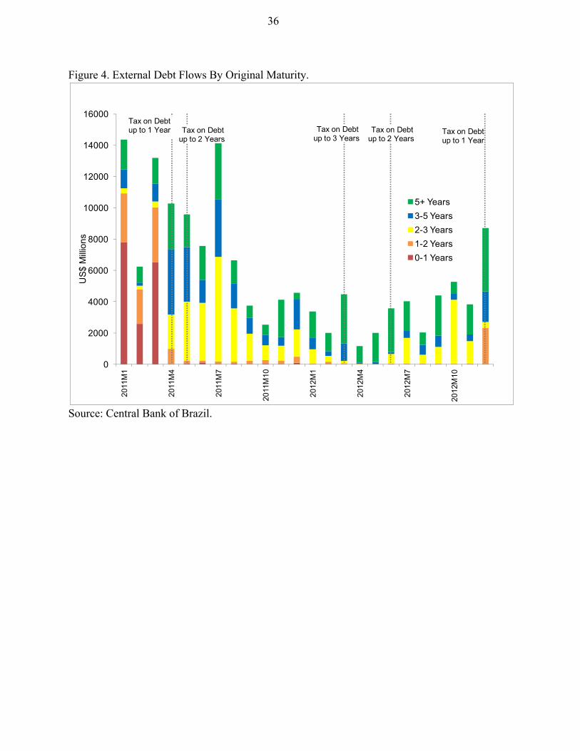
36

Figure 4. External Debt Flows By Original Maturity.

Source: Central Bank of Brazil.

0

2000

4000

6000

8000

10000

12000

14000

1600020

11M

1

2011

M4

2011

M7

2011

M10

2012

M1

2012

M4

2012

M7

2012

M10

US

$ M

illio

ns

5+ Years

3-5 Years

2-3 Years

1-2 Years

0-1 Years

Tax on Debtup to 1 Year Tax on Debt

up to 3 Years Tax on Debt

up to 2 Years Tax on Debtup to 1 Year

Tax on Debtup to 2 Years

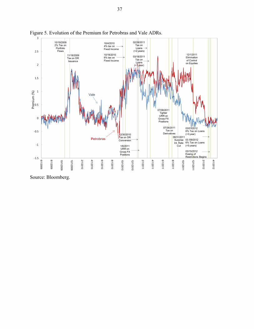
37

Figure 5. Evolution of the Premium for Petrobras and Vale ADRs.

Source: Bloomberg.

0

10

20

30

40

50

60

70

80

90

100

-1.5

-1

-0.5

0

0.5

1

1.5

2

2.5

3

6/1/2009

8/1/2009

10/1/2009

12/1/2009

2/1/2010

4/1/2010

6/1/2010

8/1/2010

10/1/2010

12/1/2010

2/1/2011

4/1/2011

6/1/2011

8/1/2011

10/1/2011

12/1/2011

2/1/2012

4/1/2012

Prem

ium

(%)

Petrobras

Vale

10/19/20092% Tax on Portfolio Flows

11/18/2009Tax on DR Issuance

12/1/2011Eliminationof Control on Equities

07/08/2011Tighter URR on

Gross FX Positions

10/4/20104% tax on Fixed Income

10/18/20106% tax onFixed Income

02/28/2011Tax on Loans

(<2 years)

03/18/2011Tax on Loans

(<1 year)

12/30/2010Tax on DR Conversion

1/6/2011URR on

Gross FXPositions

07/26/2011Tax on

Derivatives

03/01/20126% Tax on Loans(<3 year)

03 /09/20126% Tax on Loans(<5 years)

03/15/2012Easing of Restrictions Begins

08/31/2011SurpriseInt. Rate

Cut

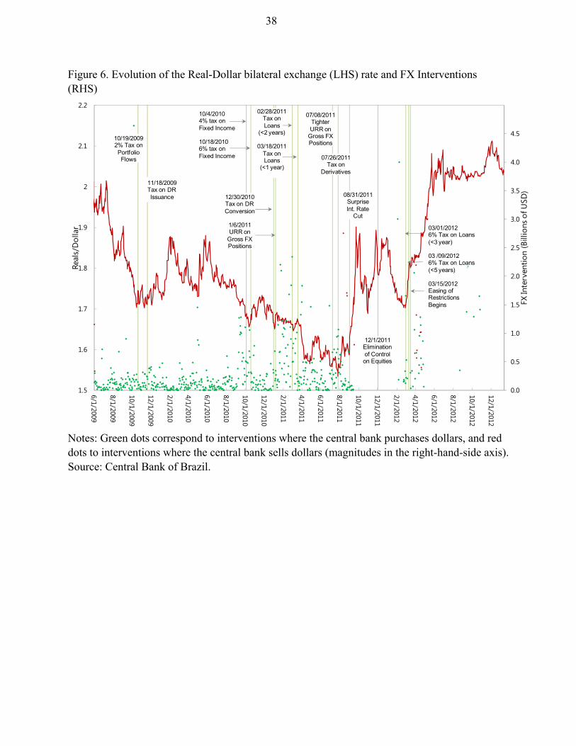
38

Figure 6. Evolution of the Real-Dollar bilateral exchange (LHS) rate and FX Interventions (RHS)

Notes: Green dots correspond to interventions where the central bank purchases dollars, and red dots to interventions where the central bank sells dollars (magnitudes in the right-hand-side axis). Source: Central Bank of Brazil.

0.0

0.5

1.0

1.5

2.0

2.5

3.0

3.5

4.0

4.5

1.5

1.6

1.7

1.8

1.9

2

2.1

2.2

6/1/2009

8/1/2009

10/1/2009

12/1/2009

2/1/2010

4/1/2010

6/1/2010

8/1/2010

10/1/2010

12/1/2010

2/1/2011

4/1/2011

6/1/2011

8/1/2011

10/1/2011

12/1/2011

2/1/2012

4/1/2012

6/1/2012

8/1/2012

10/1/2012

12/1/2012

FX In

terv

entio

n (B

illio

ns o

f USD

)

Real

s/D

olla

r

10/19/20092% Tax on Portfolio Flows

11/18/2009Tax on DR Issuance

12/1/2011Eliminationof Control on Equities

03/01/20126% Tax on Loans(<3 year)

03 /09/20126% Tax on Loans(<5 years)

03/15/2012Easing of Restrictions Begins

07/08/2011Tighter URR on

Gross FX Positions

10/4/20104% tax on Fixed Income

10/18/20106% tax onFixed Income

02/28/2011Tax on Loans

(<2 years)

03/18/2011Tax on Loans

(<1 year)

12/30/2010Tax on DR Conversion

1/6/2011URR on

Gross FXPositions

07/26/2011Tax on

Derivatives

08/31/2011SurpriseInt. Rate

Cut

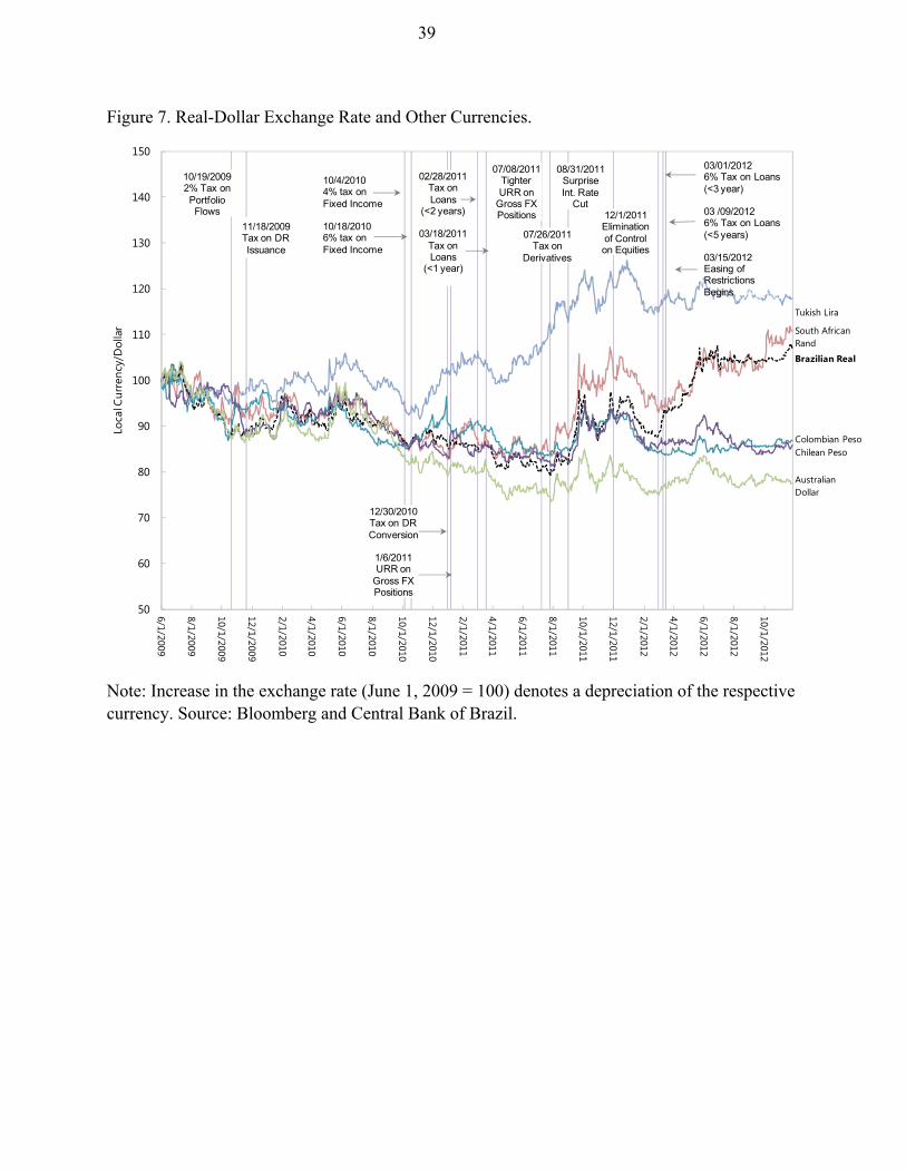
39

Figure 7. Real-Dollar Exchange Rate and Other Currencies.

Note: Increase in the exchange rate (June 1, 2009 = 100) denotes a depreciation of the respective currency. Source: Bloomberg and Central Bank of Brazil.

50

60

70

80

90

100

110

120

130

140

150

6/1/2009

8/1/2009

10/1/2009

12/1/2009

2/1/2010

4/1/2010

6/1/2010

8/1/2010

10/1/2010

12/1/2010

2/1/2011

4/1/2011

6/1/2011

8/1/2011

10/1/2011

12/1/2011

2/1/2012

4/1/2012

6/1/2012

8/1/2012

10/1/2012

Loca

l Cur

renc

y/D

olla

r South AfricanRand

Colombian Peso

Brazilian Real

AustralianDollar

Tukish Lira

Chilean Peso

10/19/20092% Tax on Portfolio Flows

11/18/2009Tax on DR Issuance

12/1/2011Eliminationof Control on Equities

03/01/20126% Tax on Loans(<3 year)

03 /09/20126% Tax on Loans(<5 years)

03/15/2012Easing of Restrictions Begins

07/08/2011Tighter URR on

Gross FX Positions

10/4/20104% tax on Fixed Income

10/18/20106% tax onFixed Income

02/28/2011Tax on Loans

(<2 years)

03/18/2011Tax on Loans

(<1 year)

12/30/2010Tax on DR Conversion

1/6/2011URR on

Gross FXPositions

07/26/2011Tax on

Derivatives

08/31/2011SurpriseInt. Rate

Cut

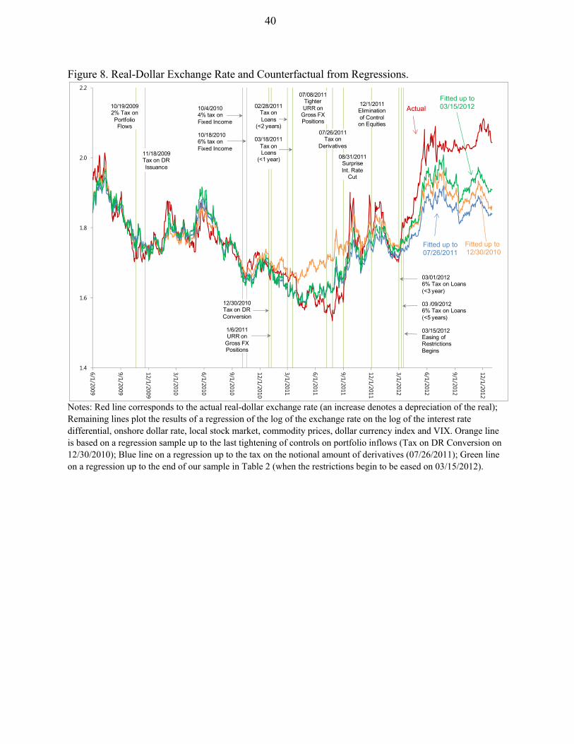
40

Figure 8. Real-Dollar Exchange Rate and Counterfactual from Regressions.

Notes: Red line corresponds to the actual real-dollar exchange rate (an increase denotes a depreciation of the real); Remaining lines plot the results of a regression of the log of the exchange rate on the log of the interest rate differential, onshore dollar rate, local stock market, commodity prices, dollar currency index and VIX. Orange line is based on a regression sample up to the last tightening of controls on portfolio inflows (Tax on DR Conversion on 12/30/2010); Blue line on a regression up to the tax on the notional amount of derivatives (07/26/2011); Green line on a regression up to the end of our sample in Table 2 (when the restrictions begin to be eased on 03/15/2012).

1.4

1.6

1.8

2.0

2.2

6/1/2009

9/1/2009

12/1/2009

3/1/2010

6/1/2010

9/1/2010

12/1/2010

3/1/2011

6/1/2011

9/1/2011

12/1/2011

3/1/2012

6/1/2012

9/1/2012

12/1/2012

10/19/20092% Tax on Portfolio Flows

11/18/2009Tax on DR Issuance

12/1/2011Eliminationof Control on Equities

03/01/20126% Tax on Loans(<3 year)

03 /09/20126% Tax on Loans(<5 years)

03/15/2012Easing of Restrictions Begins

07/08/2011Tighter URR on

Gross FX Positions

10/4/20104% tax on Fixed Income

10/18/20106% tax onFixed Income

02/28/2011Tax on Loans

(<2 years)

03/18/2011Tax on Loans

(<1 year)

12/30/2010Tax on DR Conversion

1/6/2011URR on

Gross FXPositions

07/26/2011Tax on

Derivatives

Actual

Fitted up to03/15/2012

Fitted up to07/26/2011

Fitted up to 12/30/2010

08/31/2011SurpriseInt. Rate

Cut

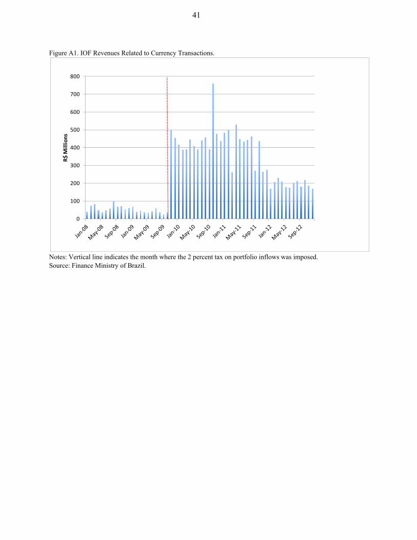
41

Figure A1. IOF Revenues Related to Currency Transactions.

Notes: Vertical line indicates the month where the 2 percent tax on portfolio inflows was imposed. Source: Finance Ministry of Brazil.

0

100

200

300

400

500

600

700

800

R$

Mil

lio

ns