1

Capelin: Data-Driven Capacity Procurement forCloud Datacenters using Portfolios of Scenarios

[Technical Report on the TPDS homonym article]Georgios Andreadis, Fabian Mastenbroek, Vincent van Beek, and Alexandru Iosup

Abstract—Cloud datacenters provide a backbone to our digital society. Inaccurate capacity procurement for cloud datacenters canlead to significant performance degradation, denser targets for failure, and unsustainable energy consumption. Although this activity iscore to improving cloud infrastructure, relatively few comprehensive approaches and support tools exist for mid-tier operators, leavingmany planners with merely rule-of-thumb judgement. We derive requirements from a unique survey of experts in charge of diversedatacenters in several countries. We propose Capelin, a data-driven, scenario-based capacity planning system for mid-tier clouddatacenters. Capelin introduces the notion of portfolios of scenarios, which it leverages in its probing for alternative capacity-plans. Atthe core of the system, a trace-based, discrete-event simulator enables the exploration of different possible topologies, with support forscaling the volume, variety, and velocity of resources, and for horizontal (scale-out) and vertical (scale-up) scaling. Capelin comparesalternative topologies and for each gives detailed quantitative operational information, which could facilitate human decisions ofcapacity planning. We implement and open-source Capelin, and show through comprehensive trace-based experiments it can aidpractitioners. The results give evidence that reasonable choices can be worse by a factor of 1.5-2.0 than the best, in terms ofperformance degradation or energy consumption.

Index Terms—Cloud, procurement, capacity planning, datacenter, practitioner survey, simulation

F

1 INTRODUCTION

C LOUD datacenters are critical for today’s increasinglydigital society [20, 22, 23]. Users have come to expect

near-perfect availability and high quality of service, at lowcost and high scalability. Planning the capacity of cloud in-frastructure is a critical yet non-trivial optimization problemthat could lead to significant service improvements, costsavings, and environmental sustainability [4]. This activityincludes short-term capacity planning, which includes theprocess of provisioning and allocating resources from thecapacity already installed in the datacenter, and long-termcapacity planning, which is the process of procuring machinesthat form the datacenter capacity. This work focuses onthe latter, which is a process involving large amounts ofresources and decisions that are difficult to reverse.

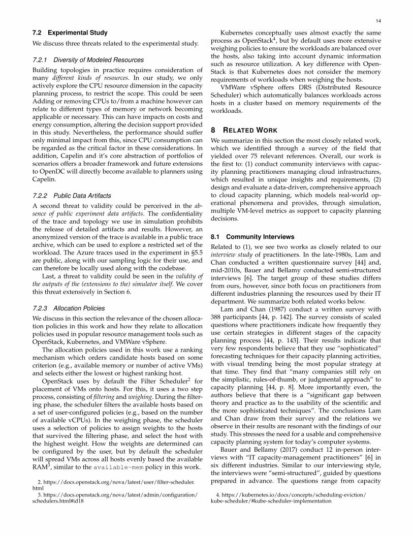
Although many approaches to the long-term capacity-planning problem have been published [13, 53, 66], com-panies use much rule-of-thumb reasoning for procurementdecisions. To minimize operational risks, many such indus-try approaches currently lead to significant overprovision-ing [25], or miscalculate the balance between underprovi-sioning and overprovisioning [49]. In this work, as Figure 1depicts, we approach the problem of capacity planning formid-tier cloud datacenters with a semi-automated, special-ized, data-driven tool for decision making.

We focus in this work mainly on mid-tier providers ofcloud infrastructure that operate at the low- to mid-leveltiers of the service architecture, ranging from IaaS to PaaS.

• G. Andreadis, F. Mastenbroek, V. van Beek, and A. Iosup are with Electri-cal Engineering, Mathematics & Computer Science, Delft University ofTechnology, 2628 CD Delft, Netherlands.

• V. van Beek is also with Solvinity, 1100 ED Amsterdam, Netherlands.• A. Iosup is also with Computer Science, Vrije Universiteit Amsterdam,

1081 HV Amsterdam, Netherlands.

ClusterClusterClusterClusterClusterCluster

VMs

VMsVMs

{…}

Current Practice Capelin (this work)

Capelin (§4)

VM

Workloads

VMsVMsHost

Topology

VMsVMsData

Monitoring

VMsVMsHost VMsHost

generic, coarse-grained right-sized, fine-grained

Data Filter (§5)

Portfolios

{…}

ClusterClusterCluster

VMsVMsVMsHostVMsVMsVMsHostVMsVMsVMsHost

VMsVMsVMsHost

VMsVMsVMsHostVMsVMsVMsHost

VMsVMsVMsHostH

ost

Hos

t

Capacity Planning Committee (§3)

1

3

4

4

2

3

Simulator

all dataall data

Capacity Planner (§3)

decision

decision

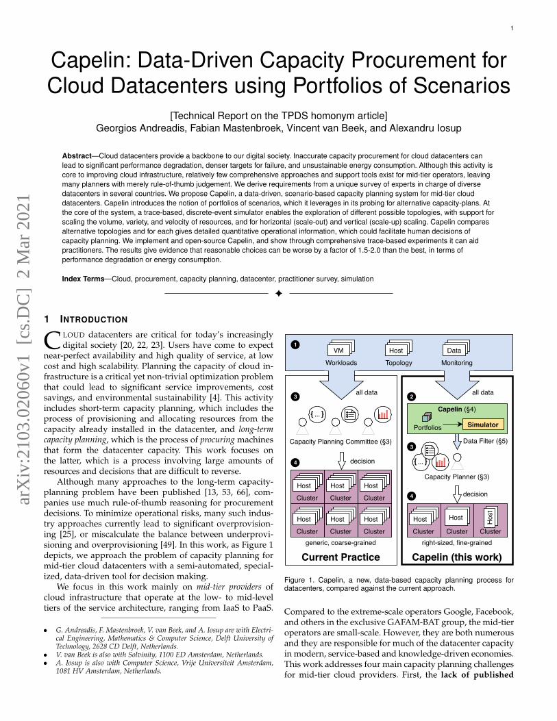
Figure 1. Capelin, a new, data-based capacity planning process fordatacenters, compared against the current approach.

Compared to the extreme-scale operators Google, Facebook,and others in the exclusive GAFAM-BAT group, the mid-tieroperators are small-scale. However, they are both numerousand they are responsible for much of the datacenter capacityin modern, service-based and knowledge-driven economies.This work addresses four main capacity planning challengesfor mid-tier cloud providers. First, the lack of published

arX

iv:2

103.

0206

0v1

[cs

.DC

] 2

Mar

202

1

2

knowledge about the current practice of long-term cloudcapacity planning. For a problem of such importance andlong-lasting effects, it is surprising that the only studiesof how practitioners make and take long-term capacity-planning decisions are either over three decades old [44]or focus on non-experts deciding how to externally procurecapacity for IT services [6]. A survey of expert capacityplanners could reveal new requirements.

Second, we observe the need for a flexible instrumentfor long-term capacity planning, one that can address var-ious operational scenarios. State-of-the-art tools [30, 34, 62]and techniques [13, 24, 57] for capacity-planning operateon abstractions that match only one vendor or focus onsimplistic problems. Although single-vendor tools, such asVMware’s Capacity Planner [62] and IBM’s Z Performanceand Capacity Analytics tool [34], can provide good advicefor the cloud datacenters equipped by that vendor, they donot support real-world cloud datacenters that are heteroge-neous in both software [2][4, §2.4.1] and hardware [10, 18][4,§3]. Yet, to avoid vendor lock-in and licensing costs, clouddatacenters acquire heterogeneous hardware and softwarefrom multiple sources and could, for example, combineVMware’s, Microsoft’s, and open-source OpenStack+KVMvirtualization management technology, and complementit with container technologies. Although linear program-ming [63], game theory [57], stochastic search [24], andother optimization techniques work well on simplisticcapacity-planning problems, they do not address the multi-disciplinary, multi-dimensional nature of the problem. AsFigure 1 (left) depicts, without adequate capacity planningtools and techniques, practitioners need to rely on rules-of-thumb calibrated with casual visual interpretation of thecomplex data provided datacenter monitoring. This state-of-practice likely results in overprovisioning of cloud data-centers, to avoid operational risks [26]. Even then, evolvingcustomers and workloads could make the planned capacityinsufficient, leading to risks of not meeting Service LevelAgreements [1, 7], inability to absorb catastrophic failures [4,p.37], and even unwillingness to accept new users.

Third, we identify the need for comprehensive evalu-ations of long-term capacity-planning approaches, basedon real-world data and scenarios. Existing tools and tech-niques have rarely been tested with real-world scenarios,and even more rarely with real-world operational traces thatcapture the detailed arrival and execution of user requests.Furthermore, for the few thus tested, the results are onlyrarely peer-reviewed [1, 53]. We advocate comprehensiveexperiments with real-world operational traces and diversescaling scenarios to test capacity planning approaches.

Fourth and last, we observe the need for publiclyavailable, comprehensive tools for long-term capacityplanning. However, and in stark contrast with the manyavailable tools for short-term capacity planning, few pro-curement tools are publicly available, and even fewer areopen-source. From the available tools, none can model allthe aspects needed to analyze cloud datacenters from §2.

We propose in this work Capelin, a data-driven,scenario-based alternative to current capacity planning ap-proaches. Figure 1 visualizes our approach (right columnof the figure) and compares it to current practice (leftcolumn). Both approaches start with inputs such as work-

loads, current topology, and large volumes of monitoringdata (step 1 in the figure). From this point on, the twoapproaches diverge, ultimately resulting in qualitativelydifferent solutions. The current practice expects a committeeof various stakeholder to extract meaning from all the inputdata ( 3 ), which is severely hampered by the lack of decisionsupport tools. Without a detailed understanding of theimplications of various decisions, the final decision is takenby committee, and it is typically an overprovisioned andconservative approach ( 4 ). In contrast, Capelin adds andsemi-automates a data-driven approach to data analysis anddecision support ( 2 ), and enables capacity planners to takefine-grained decisions based on curated and greatly reduceddata ( 3 ). With such support, even a single capacity plan-ner can make a tailored, fine-grained decision on topologychanges to the cloud datacenter ( 4 ). More than a purelytechnical solution, this approach can change organizationalprocesses. Overall, our main contribution is:

1) We design, conduct, and analyze community interviewson capacity planning in different cloud settings (Sec-tion 3). We use broad, semi-structured interviews, fromwhich we identify new, real-world requirements.

2) We design Capelin, a semi-automated, data-driven ap-proach for long-term capacity planning in cloud datacen-ters (Section 4). At the core of Capelin is an abstraction,the capacity planning portfolio, which expresses sets of“what-if” scenarios. Using simulation, Capelin estimatesthe consequences of alternative decisions.

3) We demonstrate Capelin’s ability to support capacityplanners through experiments based on real-world op-erational traces and scenarios (Section 5). We implementa prototype of Capelin as an extension to OpenDC,an open-source platform for datacenter simulation [36].We conduct diverse trace-based experiments. Our ex-periments cover four different scaling dimensions, andworkloads from both private and public clouds. They alsoconsider different operational factors such as the sched-uler allocation policy, and phenomena such as correlatedfailures and performance interference [42, 60, 64].

4) We release our prototype of Capelin, consisting of ex-tensions to OpenDC 2.0 [46], as Free and Open-SourceSoftware (FOSS), for practitioners to use. Capelin is engi-neered with professional, modern software developmentstandards and produces reproducible results.

2 A SYSTEM MODEL FOR DC OPERATIONS

In this work we assume the generic model of cloud infras-tructure and its operation depicted by Figure 2 (next page).

Workload: The workload consists of applications execut-ing in Virtual Machines (VMs) and containers. The emphasisof this study is on business-critical workloads, which arelong-running, typically user-facing, and back-end enterpriseservices at the core of an enterprise’s business [55, 56]. Theirdowntime, or even just low Quality of Service (QoS), canincur significant and long-lasting damage to the business.We also consider virtual public cloud workloads in this model,submitted by a wider user base.

The business-critical workloads we consider also includevirtualized High Performance Computing (HPC) parts.

3

ClusterClusterCluster

HostHostHost

VM / ContainerVM / Container

Hypervisor

Workload andResource Manager

VM / Container

Application

VM / ContainerVM / ContainerHPC Tasks

Business-CriticalWorkloads

Batch Bag ofHPC Tasks

VM / ContainerVM / ContainerSpark/ML

App ManagersWorkload

RM&S

Infrastructure

VM / ContainerVM / ContainerVM / Container

Application

Cap

acity

Pla

nnin

g

Figure 2. Generic model for datacenter operation.

These are primarily comprised of conveniently (embarrass-ingly) parallel tasks, e.g., Monte Carlo simulations, formingbatch bags-of-tasks. Larger HPC workloads, such as scientificworkloads from healthcare, also fit in our model.

Our system model also considers app managers, suchas the big data frameworks Spark and Apache Flink, andmachine learning frameworks such as TensorFlow, whichorchestrate virtualized workflows and dataflows.

Infrastructure: The workloads described earlier run onphysical datacenter infrastructure. Our model views data-center infrastructure as a set of physical clusters of possiblyheterogeneous hosts (machines), each host being a node in adatacenter rack. A host can execute multiple VM or con-tainer workloads, managed by a hypervisor. The hypervisorallocates computational time on the CPU between the work-loads that request it, through time-sharing (if on the samecores) or space-sharing (if on different cores).

We model the CPU usage of applications for discretizedtime slices. Per slice, all workloads report requested CPUtime to the hypervisor and receive the granted CPU timethat the resources allow. We assume a generic memorymodel, with memory allocation constant over the runtime ofa VM. As is common in industry, we allow overcommissionof CPU resources [5], but not of memory resources [55].

Infrastructure phenomena: Cloud datacenters are com-plex hardware and software ecosystems, in which com-plex phenomena emerge. We consider in this work twowell-known operational phenomena, performance variabil-ity caused by performance interference between collocatedVMs [42, 43, 60] and correlated cluster failures [8, 19, 21].

Live Platform Management (RM&S in Figure 2): Wemodel a workload and resource manager that performsmanagement and control of all clusters and hosts, and is re-sponsible for the lifecycle of submitted VMs, including theirplacement onto the available resources [3]. The resourcemanager is configurable and supports various allocation poli-cies, defining the distribution of workloads over resources.

The devops team monitors the system and responds toincidents that the resource management system cannot self-manage [7].

Capacity Planning: Closely related with infrastructureand live platform management is the activity of capacityplanning. This activity is conducted periodically and/orat certain events by a capacity planner (or committee).The activity typically consists of first modeling the currentstate of the system (including its workload and infrastruc-ture) [47], forecasting future demand [14], deriving a capacitydecision [65], and finally calibrating and validating the deci-sion [40]. The latter is done for QoS, possibly expressed asdetailed Service Level Agreements (SLAs) and Service LevelObjectives (SLOs). In Section 3 we analyze the current stateof practice and in Section 8 we discuss existing approachesin literature.

Which cloud datacenters are relevant for this model?We focus in this work on capacity planning for mid-tiercloud infrastructures, characterized by relatively small-scalecapacity, temporary overloads being common, and a lackof in-house tools or teams large enough to develop themquickly. In Section 3 we analyze the current state of thecapacity planning practice in this context and in Section 8we discuss existing approaches in related literature.

Which tools support this model? We are not aware ofanalytical tools that can cope with these complex aspects.Although tools for VM simulation exist [12, 31, 50], few sup-port CPU over-commissioning and none outputs detailedVM-level metrics; the same happens for infrastructure phe-nomena. From the few industry-grade procurement toolswho published details about their operation, none supportsthe diverse workloads and phenomena considered here.

3 REAL-WORLD EXPERIENCES WITH CAPACITYPLANNING IN CLOUD INFRASTRUCTURES

Real-world practice can deviate significantly from publishedtheories and strategies. In this section, we conduct andanalyze interviews with 8 practitioners from a wide range ofbackgrounds and multiple countries, to assess whether thisis the case in the field of capacity planning.

3.1 MethodOur goal is to collect real-world experiences from practition-ers systematically and without bias, yet also leave room forflexible, personalized lines of investigation.

3.1.1 Interview typeThe choice of interview type is guided by the trade-offbetween the systematic and flexible requirements. A textsurvey, for example, is highly suited for a systematic study,but generally does not allow for low-barrier individualfollow-up questions or even conversations. An in-personinterview without pre-defined questions allows full flexi-bility, but can result in unsystematic results. We use thegeneral interview guide approach [58], a semi-structured typeof interview that ensures certain key topics are covered butpermits deviations from the script. We conduct in-personinterviews with a prepared script of ranked questions, andallow the interviewer the choice of which scripted questionsto use and when to ask additional questions.

4

Table 1Summary of interviews. (Notation: TTD = Time to Deploy, CP = Cloud Provider, DC = Datacenter, M = Monitoring, m/y = month/year, NIT =

National IT Infrastructure Provider, SA = Spreadsheet Analysis.)

Int. Role(s) Backgr. Scale Scope Tooling Workload Comb. Frequency TTD

1 Researcher CP rack multi-DC M combined 3m, ad-hoc ?2 Board Member NIT iteration multi-DC – combined 4–5y 12–18m3 Manager, Platform Eng. CP rack multi-DC M combined ad-hoc 4–5m4 Manager NIT iteration per DC M benchmark 6–7y 18m5 Hardware Eng. NIT iteration per DC M benchmark 6y 18m6 Researcher NIT rack multi-DC M separate 6m 12m7 Manager NIT iteration multi-DC M, SA combined 5y 3.5-4y

3.1.2 Data collectionOur data collection process involves three steps. Firstly, weselected and contacted a broad set of prospective intervieweesrepresenting various kinds of datacenters, with diverse rolesin the process of capacity planning, and with diverse re-sponsibility in the decisions.

Secondly, we conducted and recorded the interviews. Eachinterview is conducted in person and digitally recordedwith the consent of the interlocutor. Interviews last be-tween 30 and 60 minutes, depending on availability ofthe interlocutors and complexity of the discussion. To helpthe interviewer select questions and fit in the time-limitsimposed by each interviewee, we rank questions by theirimportance and group questions broadly into 5 categories:(1) introduction, (2) process, (3) inside factors, (4) outsidefactors, and (5) summary and followup. The choice betweenquestions is then dynamically adjusted to give precedence tohigher-priority questions and to ensure each category is cov-ered at least briefly. The script itself is listed in Appendix A.

Thirdly, the recordings are manually transcribed into afull transcript to facilitate easy analysis. Because mattersdiscussed in these interviews may reveal sensitive opera-tional details about the organisations of our interviewees,all interview materials are handled confidentially. No infor-mation that could reveal the identity of the interlocutor orthat could be confidential to an organization’s operations isshared without the explicit consent of the interlocutor. Inaddition, all raw records will be destroyed directly after thisstudy.

3.1.3 Analysis of InterviewsDue to the unstructured nature of the chosen interviewapproach, we combine a question-based aggregated anal-ysis with incidental findings. Our approach is inspired bythe Grounded Theory strategy set forth by Coleman andO’Connor [15], and has two steps. First, for each transcript,we annotate each statement made based on which questionsit is relevant to. This may be a sub-sentence remark or anentire paragraph of text, frequently overlapping betweendifferent questions. We augment this systematic analysiswith more general findings, including comments on unan-ticipated topics.

Secondly, we traverse all transcripts for each questionand form aggregate observations for each question in the tran-script. Appendix B details the full findings. From these, wesynthesize Capelin requirements (§4.1).

3.2 Observations from the InterviewsTable 1 summarizes the results of the interviews. In total,we transcribed over 35,000 words in 3 languages, which is a

very large amount of raw interview data. We conducted 7 in-terviews with practitioners from commercial and academicdatacenters, with roles ranging from capacity planners, todatacenter engineers, to managers. We summarize here ourmain observations:O1: A majority of practitioners find that the process in-volves a significant amount of guesswork and human inter-pretation (see detailed finding (IF16) in App. B). Interlocu-tors managing commercial infrastructures emphasize multi-disciplinary challenges such as lease and support contracts,and personnel considerations (IF19, IF18).O2: In all interviews, we notice the absence of any dedicatedtooling for the capacity planning process (IF44). Instead, thesurveyed practitioners rely on visual inspection of data,through monitoring dashboards (IF45). We observe twomain reasons for not using dedicated tooling: (1) toolstend to under-represent the complexity of the real situation,and (2) have high costs with many additional, unwantedfeatures (IF47).O3: The organizations using these capacity planning ap-proaches provide a range of digital services, ranging fromgeneral IT services to specialist hardware hosting (IF2).They run VM workloads, in both commercial and scientificsettings, and batch and HPC workloads, mainly in scientificsettings (IF3).O4: A large variety of factors are taken into account whenplanning capacity (IF34). The three named in a majorityof interviews are (1) the use of historical monitoring data,(2) financial concerns, and (3) the lifetime and aging ofhardware (IF35).O5: Success and failure in capacity planning are underspeci-fied. Definitions of success differ: two interviewees see theuse of new technologies as a success (IF6), and one interpretsthe absence of total failure events as a success (IF5). Chal-lenges include chronic underutilization (IF8), increasingcomplexity (IF9), and small workloads (IF10). Failures in-clude decisions taking long (IF12), misprediction (IF13), andnew technology having unforeseen consequences (IF11).O6: The frequency of capacity planning processes seems correlatedwith the duration of core activities using it: commercial cloudsdeploy within 4-5 months from the start of capacity plan-ning, whereas scientific clouds take 1–1.5 years (IF39, IF40).O7: We found three financial and technical factors that play arole in capacity planning: (1) funding concerns, (2) specialhardware requests, and (3) the cost of new hardware (IF74).In two interviews, interlocutors state that financial consid-erations prime over the choice of technology, such as thevendor and model (IF78).O8: The human aspect of datacenter operations is emphasizedin 5 of the 7 interviews (IF85). The datacenter administra-

5

Simulator

Legend

Capelin

Frontend

Infrastructure

Backend

Monitoring ServiceSimulator

Database

Backend

Frontend

Resource Topology

Workload

Library ofComponents

Scenario PortfolioGenerator

Capacity PlanGenerator

CapacityPlanner Scenario Portfolio

BuilderScenario Portfolio

Evaluator

Control Data Stateful

Workload Modeler

Portfolio

D

C F

EA

BG

H

I

J M

L

K

Users

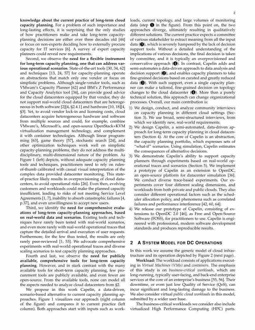
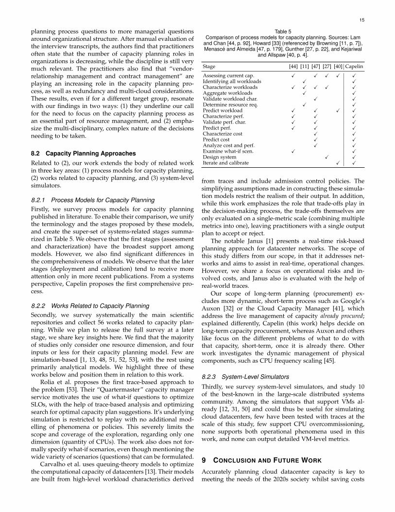
Figure 3. An overview of the architecture of Capelin. Capelin is provided information on the current state of the infrastructure and assists the capacityplanner in making capacity planning decisions. Labels indicate the order of traversal by the capacity planner (e.g., the first step is to use componentA , the scenario portfolio builder).

tors need training (IF81), and wrong decisions in capacityplanning lead to stress within the operational teams (IF83).Users also need training, to leverage heterogeneous or newresources (IF81).O9: We observe a wide range of requirements and wishesexpressed by interlocutors about custom tools for the process.Fundamentally, the tool should help manage the increasingcomplexity faced by capacity planners (IF97). A key require-ment for any tool is interactivity: practitioners want to beable to interact with the metrics they see and ask questionsfrom the tool during capacity planning meetings (IF95).The tool should be affordable and usable without needingthe entire toolset of the vendor (IF96). One intervieweeasks for support for infrastructure heterogeneity, to supportscientific computing (IF98).O10: Two interviewees detail “what-if” scenarios they wouldlike to explore with a tool, using several dimensions (IF101):(1) the topology, in the form of the computational and mem-ory capacity needed, or new hardware arriving; (2) the work-load, and especially emerging kinds; and (3) the operationalphenomena, such as failures and the live management of theplatform (e.g., scheduling and fail-over scenarios).

4 DESIGN OF CAPELIN: A CAPACITY PLANNINGSYSTEM FOR CLOUD INFRASTRUCTURE

In this section, we synthesize requirements and designaround them a capacity planning approach for cloud in-frastructure. We propose Capelin, a scenario-based capacityplanning system that helps practitioners understand the im-pact of alternatives. Underpinning this process, we proposeas core abstraction the portfolio of capacity planning scenarios.

4.1 Requirements AnalysisIn this section, from the results of Section 3, we synthesizethe core functional requirements addressed by Capelin. In-stead of aiming for full automation – a future objective thatis likely far off for the field of capacity planning – the em-phasis here is on human-in-the-loop decision support [37,P2].(FR1) Model a cloud datacenter environment (see O2, O3,

O7, and O9): The system should enable the user tomodel the datacenter topology and virtualized work-loads introduced in Section 2.

(FR2) Enable expression of what-if scenarios (see O2,O10): Users can express what-if scenarios with diversetopologies, failures, and workloads. The system shouldthen execute the what-if scenario(s), and produce andjustify a set of user-selected QoS metrics.

(FR3) Enable expression of QoS requirements, in the formof SLAs, consisting of several SLOs (see O2, O5, O9).These requirements are formulated as thresholds orranges of acceptable values for user-selected metrics.

(FR4) Suggest a portfolio of what-if scenarios, based onuser-submitted workload traces, given topology, andspecified QoS requirements (see O2, O10). This greatlysimplifies identifying meaningful scenarios.

(FR5) Provide and explain a capacity plan, optimizing forminimal capacity within acceptable QoS levels, as spec-ified by FR4 (see O2, O9). The system should explainand visualize the data sources it used to make the plan.

4.2 Overview of the Capelin ArchitectureOn the previous page, Figure 3 depicts an overview of theCapelin architecture. Capelin extends OpenDC, an open-source, discrete event simulator with multiple years of de-velopment and operation [36]. We now discuss each maincomponent of the Capelin architecture, taking the perspec-tive of a capacity planner. We outline the abstraction under-pinning this architecture, the capacity planning portfolios,in §4.3.

4.2.1 The Capelin ProcessThe frontend and backend of Capelin are embedded inOpenDC. This enables Capelin to leverage the simulator’sexisting platform for datacenter modeling and allows forinter-operability with other tools as they become part of thesimulator’s ecosystem. The capacity planner interacts withthe frontend of Capelin, starting with the Scenario PortfolioBuilder (component A in Figure 3), addressing FR2. Thiscomponent enables the planner to construct scenarios, usingpre-built components from the Library of Components ( B ).The library contains workload, topology, and operationalbuilding blocks, facilitating fast composition of scenarios. Ifthe (human) planner wants to modify historical workloadbehavior or anticipate future trends, the Workload Mod-eler ( C ) can model workloads and synthesize custom loads.

6

The planner might not always be aware of the full rangeof possible scenarios. The Scenario Portfolio Generator ( D )suggests customized scenarios extending the given base-scenario (FR4). The portfolios built in the builder can be ex-plored and evaluated in the Scenario Portfolio Evaluator ( E ).Finally, based on the results from this evaluation, the Capac-ity Plan Generator ( F ) suggests plans to the planner (FR5).

4.2.2 The Datacenter SimulatorIn Figure 3, the Frontend ( G ) acts as a portal, through whichinfrastructure stakeholders interact with its models and ex-periments. The Backend ( H ) responds to frontend requests,acting as intermediary and business-logic between frontend,and database and simulator. The Database ( I ) manages thestate, including topology models, historical data, simulationconfigurations, and simulation results. It receives inputsfrom the real-world topology and monitoring services, inthe form of workload traces. The Simulator ( J ) evaluatesthe configurations stored in the database and reports thesimulation results back to the database.

OpenDC [36, 46] is the simulation platform backingCapelin, enabling the capacity planner to model (FR1) andexperiment (FR5) with the cloud infrastructure, interac-tively. The software stack of this platform is composed ofa web app frontend, a web server backend, a database, anda discrete-event simulator. This kind of simulator offers agood trade-off between accuracy and performance, evenat the scale of mid-tier datacenters and with long-termworkloads.

4.2.3 InfrastructureThe cloud infrastructure is at the foundation of this archi-tecture, forming the system to be managed and planned.We consider three components within this infrastructure:The workload ( K ) submitted by users, the (logical or phys-ical) resource topology ( L ), and a monitoring service ( M ).The infrastructure follows the system model described inSection 2.

4.3 A Portfolio Abstraction for Cap. PlanningIn this section, we propose a new abstraction, which orga-nizes multiple scenarios into a portfolio (see Figure 4). Eachportfolio includes a base scenario, a set of candidate scenar-ios given by the user and/or suggested by Capelin, and a setof targets to compare scenarios. In contrast, most capacityplanning approaches in published literature are tailoredtowards a single scenario—a single potential hardware ex-pansion, a single workload type, one type of service qualitymetrics. This approach does not cover the complexities thatcapacity planners are facing (see Section 3.2). Our portfolioreflects the multi-disciplinary and multi-dimensional natureof capacity planning by including multiple scenarios and aset of targets. We describe them, in turn.

4.3.1 ScenariosA scenario represents a point in the capacity planning (data-center design) space to explore. It consists of a combinationof workload, topology, and a set of operational phenomena.Phenomena can include correlated failures, performancevariability, security breaches, etc., allowing the scenariosto more accurately capture the real-world operations. Suchphenomena are often hard to predict intuitively during

PortfolioBase Scenario

Trace ofWorkloads

TopologyConfiguration

OperationalPhenomena

Candidate ScenariosAdaptedWorkload

AdaptedTopology

OperationalPhenomena

TargetsSelectMetrics

SelectSLOs

TimeRange

Figure 4. Abstraction of a capacity planning portfolio, consisting ofa base scenario, a number of candidate scenarios, and comparisontargets.

capacity planning, due to emergent behavior that can ariseat scale.

The baseline for comparison in a portfolio is the basescenario. It represents the status quo of the infrastructureor, when planning infrastructure from scratch, it consists ofvery simple base workloads and topologies.

The other scenarios in a portfolio, called candidate scenar-ios, represent changes to the configuration that the capacityplanner could be interested in. Changes can be effected inone of the following four dimensions: (1) Variety: qualitativechanges to the workload or topology (e.g., different arrivalpatterns, or resources with more capacity); (2) Volume: quan-titative changes to the workload or topology (e.g., moreworkloads or more resources); (3) Velocity: speed-relatedchanges to workload or topology (e.g., faster resources); and(4) Vicissitude combines (1)-(3) over time.

This approach to derive candidate scenarios is system-atic, and although abstract it allows approaching many ofthe practical problems discussed by capacity planners. Forexample, an ongoing discussion is horizontal scaling (scale-out) vs. vertical (scale-up) [54]. Horizontal scaling, whichis done by adding clusters and commodity machines, con-trasts to vertical scaling, which is done by acquiring moreexpensive, “beefy” machines. Horizontal scaling is typicallycheaper for the same performance, and offers a broaderfailure-target (except for cluster-level failures). Yet, verticalscaling could lower operational costs, due to fewer per-machine licenses, fewer switch-ports for networking, andsmaller floor-space due to fewer racks. Experiment 5.2 ex-plores this dichotomy.

4.3.2 TargetsA portfolio also has a set of targets that prescribe on whatgrounds the different scenarios should be compared. Targetsinclude the metrics that the practitioner is interested in andtheir desired granularity, along with relevant SLOs (FR3).Following the taxonomy defined by the performance orga-nization SPEC [29], we support both system-provider metrics(such as operational risk and resource utilization) and or-ganization metrics (such as SLO violation rates and perfor-mance variability). The targets also include a time rangeover which these metrics should be recorded and com-pared.

7

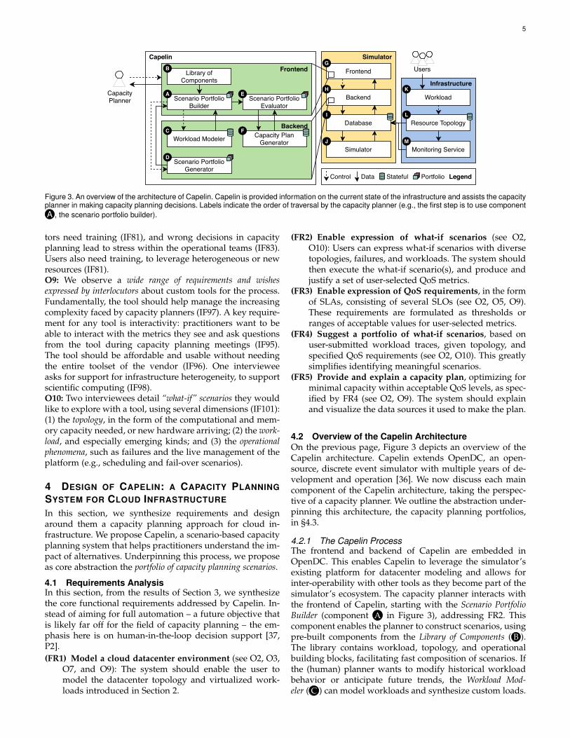
Table 2Experiment configurations. A legend of topology dimensions is provided below. (Notation: PI = Performance Interference, pub = public cloud trace,

pri = private cloud trace.)

Candidate Topologies Workloads Op. Phenomena

Sec. Focus Mode Quality Direction Variance Trace Loads Failures PI Alloc. Policy

§5.2 Hor. vs. Ver. pri sampled 3 3 active-servers

§5.3 Velocity pri sampled 3 3 active-servers

§5.4 Op. Phen. – – – – pri original 7 / 3 7 / 3 all

§5.5 Workloads pri / pub sampled 3 7 active-servers

replace

Mode QualityDirection Variance

volumehorizontalexpand velocityvertical heterogeneoushomogeneous

5 EXPERIMENTS WITH CAPELIN

In this section, we explore how Capelin can be used toanswer capacity planning questions. We conduct extensiveexperiments using Capelin and data derived from opera-tional traces collected long-term from private and publiccloud datacenters.

5.1 Experiment SetupWe implement a prototype of Capelin (§5.1.1), and verify thereproducibility of its results and that it can be run within theexpected duration of a capacity planning session (§5.1.2). Allexperiments use long-term, real-world traces as input.

Our experiment design, which Table 2 summarizes, iscomprehensive and addresses key questions such as: Whichinput workload (§5.1.3)? Which datacenter topologies toconsider (§5.1.4)? Which operational phenomena (§5.1.6)?Which allocation policy (§5.1.5)? Which user- and operator-level performance metrics to use, to compare the scenariosproposed by the capacity planner (§5.1.7)?

The most important decision for our experiments iswhich scenarios to explore. Each experiment takes in acapacity planning portfolio (see Section 4.3), starts from abase scenario, and aims to extend the portfolio with newcandidate scenarios and its results. The baseline is given byexpert datacenter engineers, and has been validated with hardwarevendor teams. Capelin creates new candidates by modifyingthe base scenario along dimensions such as variety, volume,and velocity of any of the scenario-components. In thefollowing, we experiment systematically with each of these.

5.1.1 Software prototypeWe extend the open-source OpenDC simulation plat-form [36] with capabilities for modeling and simulatingthe virtualized workloads prevalent in modern clouds. Wemodel the CPU and memory usage of each VM alongwith hypervisors deployed on each managed node. Eachhypervisor implements a fair-share scheduling model forVMs, granting each VM at least a fair share of the availableCPU capacity, but also allowing them to claim idle capacityof other VMs. The scheduler permits overprovisioning ofCPU resources, but not of memory resources, as is common inindustry practice. We also model a workload and resourcemanager that controls the deployed hypervisors and de-cides based on configurable allocation policies (describedin §5.1.5) to which hypervisor to allocate a submitted VM.Our experiments and workload samples are orchestrated by

Capelin, which is written in Kotlin (a modern JVM-basedlanguage), and processed and analyzed by a suite of toolsbased on Python and Apache Spark. More detail about thesoftware implementation is given in Appendix C.

We release our extensions of the open-source OpenDC code-base and the analysis software artifacts on GitHub1, as part ofrelease 2.0 [46]. We conduct thorough validation and testsof both the core OpenDC and our additions, as detailed inSection 6.

5.1.2 Execution and EvaluationOur results are fully reproducible, regardless of the physicalhost running them. All setups are repeated 32 times. The re-sults, in files amounting to hundreds of GB in size due to thelarge workload traces involved, are evaluated statisticallyand verified independently. Factors of randomness (e.g.,random sampling, policy decision making if applicable, andperformance interference modeling) are seeded with thecurrent repetition to ensure deterministic outcomes, and forfairness are kept consistent across scenarios.

Capelin could be used during capacity planning meet-ings. A single evaluation takes 1–2 minutes to complete,enabled by many technical optimizations we added to thesimulator. The full set of experiments is conveniently paral-lel and takes around 1 hour and 45 minutes to complete, ona “beefy” but standard machine with 64 cores and 128GBRAM; parallelization across multiple machines would re-duce this to minutes.

5.1.3 WorkloadWe experiment with a business-critical workload trace fromSolvinity, a private cloud provider. The anonymized version ofthis trace has been published in a public trace archive [35].We were provided with the full, deanonymized data arti-facts of this trace, which consists of more than 1,500 VMsalong with information on which physical resources whereused to run the trace and which VMs were allocated towhich resources. We cannot release these full traces due toconfidentiality, but release the summarized results.

The full trace includes a range of VM resource-usage mea-surements, aggregated over 5-minute-intervals over threemonths. It consumes 3,063 PFLOPs (exascale), with the meanCPU utilization on this topology of 5.6%. This low utiliza-tion is in line with industry, where utilization levels below

1. https://github.com/atlarge-research/opendc

8

Table 3Aggregate statistics for both workloads used in this study. (Notation: AP

= Solvinity.)

Characterization AP Azure

VM submissionsper hour

Mean (×10−3) 31.836 4.547CoV 134.605 17.188

VM duration [days] Mean 20.204 2.495CoV 0.378 3.072

CPU load [TFLOPs] Mean (×102) 9.826 64.046CoV 2.992 4.654

15% are common [61], and reduce the risk of not meetingSLAs.

For all experiments, we consider the full trace, andfurther generate three other kinds of workloads as sam-ples (fractions) of the original workload. These workloadsare sampled from the full trace, resulting, in turn, to 306PFLOPs (0.1 of the full trace), 766 (0.25), and 1,532 (0.5).To sample, Capelin takes randomly VMs from the full traceand adds their entire load, until the resulting workloadhas enough load. We illustrate this in pseudocode, in Al-gorithm 1.

For the §5.5 experiment, we further experiment witha public cloud trace from Azure [16]. We use the mostrecent release of the trace. The formats of the Azure andthe Solvinity traces are very similar, indicating a de factostandard has emerged across the private and public cloudcommunities. One difference in the level of anonymity ofthe trace requires an additional assumption. Whereas theSolvinity trace expresses CPU load as a frequency (MHz),the Azure trace expresses it as a utilization metric rangingfrom 0 to the number of cores of that VM. Thus, for theAzure trace, in line with Azure VM types on offer weassume a maximum frequency of 3 GHz and scale eachutilization measurement by this value. The Azure trace isalso shorter than Solvinity’s full trace, so we shorten thelatter to Azure’s length of 1 month.

We combine for the §5.5 experiment the two traces andinvestigate possible phenomena arising from their interac-tion. We disable here performance interference, because wecan only derive it for the Solvinity trace (see §5.1.6). Tocombine the two traces, we first take a random sampleof 1% from the (very large) Azure trace, which results in26,901 VMs running for one month. We then further samplethis 1%-sample, using the same method as for Solvinity’sfull trace. The full procedure is listed in Algorithm 2.

5.1.4 Datacenter topologyAs explained at the start of §5.1, for all experiments we setthe topology that ran Solvinity’s original workload (the fulltrace in §5.1.3) as the base scenario’s topology. This topologyis very common for industry practice. It is a subset of thecomplete topology of the Solvinity when the full trace wascollected, but we cannot release the exact topology or theentire workload of Solvinity due to confidentiality.

From the base scenario, Capelin derives candidate sce-narios as follows. First, it creates a temporary topologyby choosing half of the clusters in the topology, consistingof average-sized clusters and machines, compared to theoverall topology. Second, it varies the temporary topology,in four dimensions: (1) the mode of operation: replacement

(removing the original half and replacing it with the mod-ified version) and expansion (adding the modified halfto the topology and keeping the original version intact);(2) the modified quality: volume (number of machines/cores)and velocity (clock speed of the cores); (3) the direction ofmodification: horizontal (more machines with fewer coreseach) and vertical (fewer machines with more cores each);and (4) the kind of variance: homogeneous (all clusters in thetopology-half modified in the same way) and heterogeneous(two thirds in the topology-half being modified in the des-ignated way, the remaining third in the opposite way, on thedimension being investigated in the experiment).

Each dimension is varied to ensure cores and machinecounts multiply to (at least) the same total core count asbefore the change, in the modified part of the topology.For volume changes, we differentiate between a horizontalmode, where machines are given 28 cores (a standard sizefor machines in current deployments), and vertical modes,where machines are given 128 cores (the largest CPU modelswe see being commonly deployed in industry). For velocitychanges, we differentiate between the clock speed of thebase topology and a clock speed that is roughly 25% higher.Because we do not investigate memory-related effects, thetotal memory capacity is preserved.

Last, due to confidentiality, we can describe the base andderived topologies only in relative terms.

5.1.5 Allocation policiesWe consider several policies for the placement of VMs onhypervisors: (1) prioritizing by available memory (mem),(2) by available memory per CPU core (core-mem), (3) bynumber of active VMs (active-servers), (4) mimickingthe original placement data (replay), and (5) randomlyplacing VMs on hosts (random). Policies 1-3 are activelyused in production datacenters [59].

For each policy we use two variants, following theWorst-Fit strategy (selecting the resource with the most avail-able resource of that policy) and the Best-Fit strategy (theinverse, so selecting the least available, labeled with thepostfix -inv in §5.4).

5.1.6 Operational phenomenaEach capacity planning scenario can include operationalphenomena. In these experiments, we consider two suchphenomena, (1) performance variability caused by perfor-mance interference between collocated VMs, and (2) cor-related cluster failures. Both are enabled, unless otherwisementioned.

We assume a common model [42, 60] of performanceinterference, with a score from 0 to 1 for a given set of collo-cated workloads, with 0 indicating full interference betweenVMs contending for the same CPU, and 1 indicating non-interfering VMs. We derive the value from the CPU Readyfraction of a VM time-slice: the fraction of time a VM isready to use the CPU but is not able to, due to other VMsoccupying it. We mine the placement data of all VMs run-ning on the base topology and collect the set of collocatedworkloads along with their mean score, defined as the meanCPU ready time fraction subtracted from 1, conditioned bythe total host CPU load at that time, rounded to one decimal.At simulation time, this score is then activated if a VMs iscollocated with at least one of the others in the recorded set

9

Algorithm 1 Sampling procedure for the VMs in Solvinity trace (as described in §5.1.3).1: procedure SAMPLETRACE(vms, fraction, totalLoad)2: selected← ∅ . The set of selected VMs3: load← 0 . Current total load (FLOP)4: while |vms| > 0 do5: vm← Randomly removed element from vms6: vmLoad← Total load of vm7: if load+vmLoad

totalLoad > fraction then8: return selected9: end if

10: load← load + vmLoad11: selected← selected ∪ {vm}12: end while13: return selected14: end procedure

Algorithm 2 Sampling procedure for combining the private and private traces (as described in §5.1.3).1: procedure SAMPLEMULTIPLETRACES(vmsPri, fractionPri, vmsPub, fractionPub)2: Ensure VMs in vmsPri and vmsPri have same length3: vmsPub← Randomly sample 0.01 of all VMs in vmsPub4: totalLoad← Total CPU load of the private trace5: vmsPriSelected← SAMPLETRACE(vmsPri, fractionPri, totalLoad)6: vmsPubSelected← SAMPLETRACE(vmsPub, fractionPub, totalLoad)7: return vmsPriSelected ∪ vmsPubSelected8: end procedure

Table 4Parameters for the lognormal failure model we use in experiments. We

use the normal logarithm of each value.

Parameter [Unit] Scale Shape

Inter-arrival time [hour] 24× 7 2.801Duration [minute] 60 60× 8Group size [machine-count] 2 1

and the total load level on the system is at least the recordedload. The score is then applied to each collocated VMs withprobability 1/N , where N is the number of collocated VMs,by multiplying its requested CPU cycles with the score andgranting it this (potentially lower) amount of CPU time.

The second phenomenon we model are cluster failures,which are based on a common model for space-correlatedfailures [21] where a failure may trigger more failures withina short time span; these failures form a group. We consider inthis work only hardware failures that crash machines (full-stop failures), with subsequent recovery after some dura-tion. We use a lognormal model with parameters for failureinter-arrival time, group size, and duration, as listed inTable 4. The failure duration is further restricted by a min-imum of 15 minutes, since faster recoveries and reboots atthe physical level are rare. The choice of parameter values isinspired by GRID’5000 [21] (public trace also available [38])and Microsoft Philly [39], scaled to Solvinity’s topology.

5.1.7 MetricsIn our article, we use the following metrics:(1) the total requested CPU cycles (in MFLOPs) of all VMs,(2) the total granted CPU cycles (in MFLOPs) of all VMs,(3) the total overcommitted CPU cycles (in MFLOPs) of

all VMs, defined as the sum of CPU cycles that wererequested but not granted,

(4) the total interfered CPU cycles (in MFLOPs) of all VMs,defined as the sum of CPU cycles that were requestedbut could not be granted due to performance interfer-ence,

(5) the total power consumption (in Wh) of all machinesusing a linear model based on machine load [9], withan idle baseline of 200 W and a maximum power drawof 350 W,

(6) the number of time slices a VM is in a failed state,summed across all VMs.

(7) the mean CPU usage (in MHz), defined as the meannumber of granted cycles per second per machine,averaged across machines,

(8) the mean CPU demand (in MHz), defined as the meannumber of requested cycles per second per machine,averaged across machines,

(9) the mean number of deployed VM images per host,(10) the maximum number of deployed VM images per

host,(11) the total number of submitted VMs,(12) the maximum number of queued VMs in the system at

any point in time,(13) the total number of finished VMs,(14) the total number of failed VMs.

Note on the model for power consumption: The currentmodel, i.e., linear in the server load with offsets, is basedon a peer-reviewed model and common to other simulatorscommonly used in practice, such as CloudSim and GridSim,and produces in general reasonable results for CPU powerconsumption. More accurate energy models appear for ex-ample in GreenCloud and in CloudNetSim++, which modelthe dynamic energy-performance trade-off when using theDVFS technique, and in iCanCloud’s E-mc2 extension and

10

in DISSECT-CF, which model every power state of eachresource.

5.1.8 Listing of Full ResultsIn the subsections below, we highlight a small selectionof the key metrics. For full transparency, we present theentire set of metrics for each experiment in the appendices.Appendix D visualizes the full results for all metrics andAppendix E lists the full results for the two most importantmetrics in tabular form.

5.2 Horizontal vs. Vertical Resource ScalingOur main findings from this experiment are:MF1: Capelin enables the exploration of a complex trade-off

portfolio of multiple metrics and capacity dimensions.MF2: Vertically scaled topologies can improve power con-

sumption (median lower by 1.47x-2.04x) but can leadto significant performance penalties (median higherby 1.53x-2.00x) and increased chance of VM failure(median higher by 2.00x-2.71x, which is a high risk!)

MF3: Capelin reveals how correlated failures impact vari-ous topologies. Here, 147k–361k VM-slices fail.

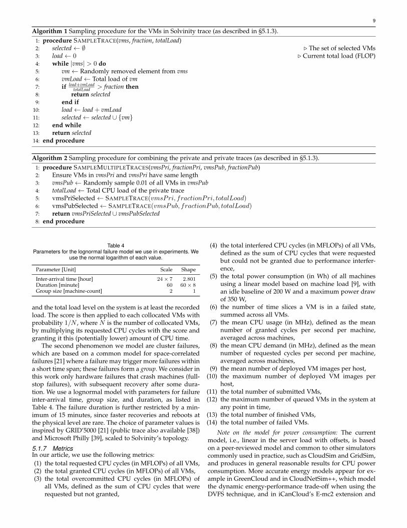
The scale-in vs. scale-out decision has historically beena challenge across the field [54][28, §1.2]. We investi-gate this decision in a portfolio of scenarios centeredaround horizontally (symbol ) vs. vertically ( ) scaled re-sources (see §5.1.4). We also vary: (1) the decision mode, byreplacing the existing infrastructure ( ) vs. expanding it ( ),and (2) the kind of variance, homogeneous resources ( )vs. heterogeneous ( ). On these three dimensions, Capelincreates candidate topologies by increasing the volume ( )and compares their performance using four workload inten-sities, two of which are shown in this analysis. We considerthree metrics for each scenario: Figure 5 (top) depicts theovercommitted CPU cycles, Figure 5 (middle) depicts thepower consumption, and Figure 5 (bottom) depicts thenumber of failed VM time slices.

Our key performance indicator is overcommitted CPUcycles, that is, the count of CPU cycles requested by VMsbut not granted, either due to collocated VMs requestingtoo many resources at once, or due to performance interfer-ence effects taking place. We observe in Figure 5 (top) thatvertically scaled topologies (symbol ) have significantlyhigher overcommission (lower performance) than their hor-izontally scaled counterparts ( , the other three symbolsidentical). The median value is higher for vertical than forhorizontal scaling, for both replaced ( ) and expanded ( )topologies, by a factor of 1.53x–2.00x (calculated as the ratiobetween medians of different scenarios at full load). Thisis a large factor, suggesting that vertically scaled topologiesare more susceptible to overcommission, and thus lead tohigher risk of performance degradation. The decrease inperformance observed in this metric is mirrored by thegranted CPU cycles metric in Figure 16b (Appendix D),which decreases for vertically scaled topologies. Amongreplaced topologies (all combinations including ), thehorizontally scaled, homogeneous topology ( ) yieldsthe best performance, and in particular the lowest me-dian overcommitted CPU. We also observe that expandedtopologies ( ) have lower overcommission than the basetopology, so adding machines is worthwhile. We observe

Figure 5. Results for a portfolio of candidate topologies and differentworkloads(§5.2): (top) overcommitted CPU cycles, (middle) total powerconsumption, (bottom) total number of time slices in which a VM is in afailed state. Table 2 describes the symbols used to encode the topology.

all these effects strongly for the full trace (3,063 PFLOPs),but less pronounced for the lower workload intensity (1,531PFLOPs).

But performance is not the only criterion for capacityplanning. We turn to power consumption, as a proxy forcost analysis and environmental concerns. We see here thatvertically scaled topologies ( ) drastically improve powerconsumption, for median values by a factor of 1.47x–2.04x,contrasting their worse performance compared to horizontalscaling ( ). As expected, all expanded topologies ( ), which

11

have more machines, incur higher power-consumption thanreplaced topologies ( ). Higher workload intensity (i.e., forthe 3,063 PFLOPs results) incurs higher power consumption,although less pronounced than earlier.

We also consider the amount of failed VM time-slices. Eachfailure here is full-stop (§5.1.6), which typically escalates analarm to engineers. Thus, this metric should be minimized.We observe significant differences here: the median failuretime of a homogeneous vertically scaled topology ( ) isbetween 2.00x–2.71x higher than the base topology. Thismetric shows similarities qualitatively with the overcom-mitted CPU cycles. Vertical scaling is correlated not onlywith worse performance, but also with higher failure counts.We see that vertical scaling leads to a significant increasein the maximum number of deployed images per physicalhost (Figure 17d), which leads to larger failure domainsand thus potentially higher failure counts. The effect isless pronounced when making heterogeneous compared tohomogeneous procurement.

Our findings show that Capelin gives practitioners thepossibility to explore a complex trade-off portfolio of dimensionssuch as power consumption, performance, failures, work-load intensity, etc. Optimization questions surrounding hor-izontal and vertical scaling can therefore be approached witha data-driven approach. We find that decisions including het-erogeneous resources can provide meaningful compromisesbetween more generic, homogeneous resources; they alsolead to different decisions related to personnel training (notshown here). We show significant differences between can-didate topologies in all metrics, translating to very differentpower costs, long-term. We conclude that Capelin can helptest intuitions and support complex decision making.

5.3 Expansion: Velocity

Our main findings from this experiment are:MF4: Capelin enables exploring a range of resource di-

mensions frequently considered in practice, such ascomponent velocity.

MF5: Increasing velocity can reduce overcommitted CPUcycles by 3.3%.

MF6: Expanding a topology by velocity can improve per-formance by 1.54x, compared to expansion by volume.

In vertical horizontal scaling, practitioners are also facedwith the decision of which qualities to scale. This experi-ment varies the velocity of resources both homogeneouslyand heterogeneously, while replacing or expanding theexisting topology. Figure 6 depicts the explored scenariosand their performance, in the form of overcommitted CPUcycles.

We find that in-place, homogeneous vertical scaling ofmachines with higher velocity leads to slightly better per-formance, by a percentage of 3.3% (compared to the basescenario, by median). In this dimension, performance variesonly slightly between homogeneously and heterogeneouslyscaled topologies, for all metrics (see also Appendix D).Expanding the topology homogeneously ( ) with a setof machines with higher CPU frequency helps reduce over-commission more drastically, also improving it beyond thelowest overcommission reached by homogeneous verticalexpansion in the previous experiment, in Figure 5. When

Figure 6. Overcommitted CPU time for a portfolio of candidate topolo-gies and different workloads, for Experiment 5.3.

Figure 7. Overcommitted CPU cycles for a portfolio of operational phe-nomena (the “none” through “all” sub-plots), and allocation policies (leg-end), for Experiment 5.4.

expanding, this cross-experiment comparison shows an im-provement of performance with a factor of 1.54x.

5.4 Impact of Operational PhenomenaOur main findings from this experiment are:MF7: Capelin enables the exploration of diverse allocation

policies and operational phenomena, both of whichlead to important differences in capacity planning.

MF8: Modeling performance interference can explain80.6%—94.5% of the overcommitted CPU cycles.

MF9: Different allocation policies lead to different perfor-mance interference intensities, and to median overcom-mitted CPU cycles different by factors between 1.56xand 30.3x compared to the best policy—high risk!

This experiment addresses operational factors in thecapacity planning process. We explore the impact of bet-ter handling of physical machine failures, the impact of(smarter) scheduler allocation policies, and the impact of(the absence of) performance interference on overall perfor-mance. Figure 7 shows the impact of different operationalphenomena on performance, for different allocation poli-cies. We observe that performance interference has a strongimpact on overcommission, dominating it compared to the

12

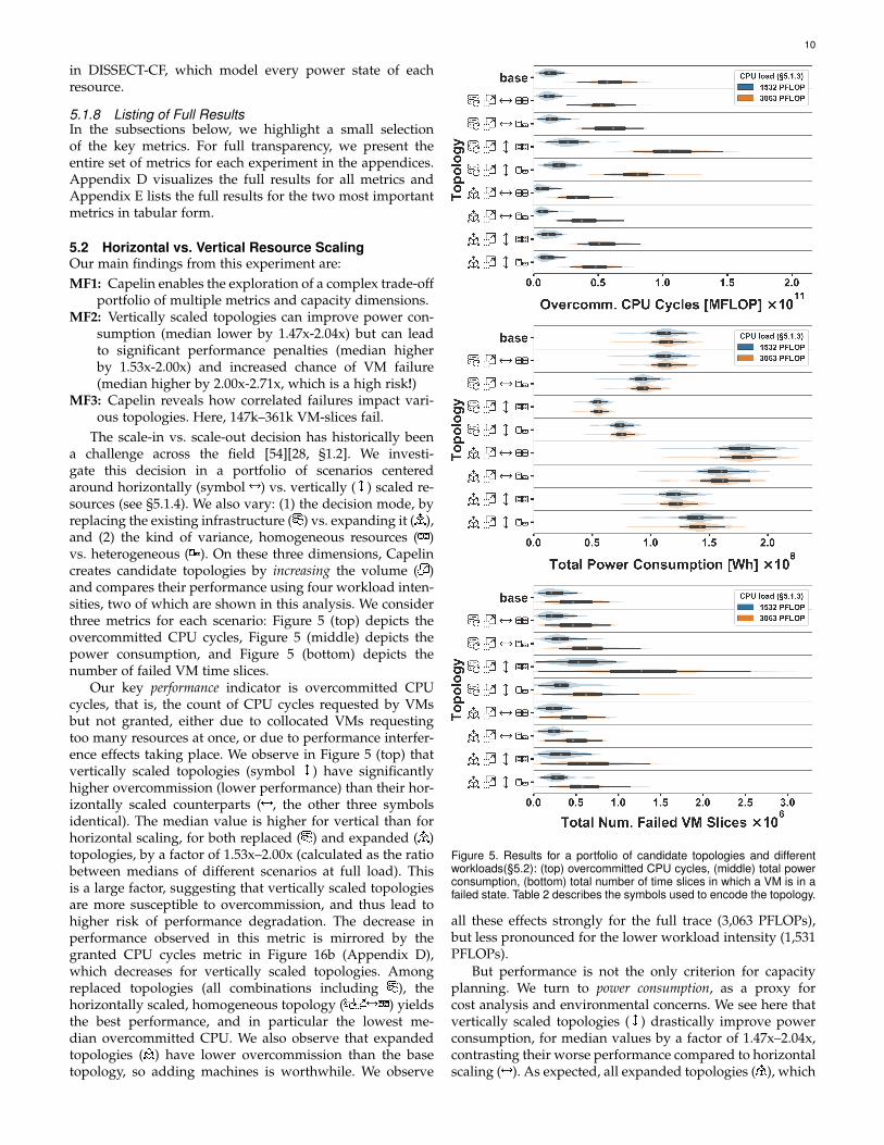
Figure 8. Total power consumption for a portfolio of candidate topologies(legend), subject to different workloads (the “all-pri” to “all-pub” sub-plots),for Experiment 5.5.

“failures” sub-plot, where only failures are considered, orwith the “none” sub-plot, where no failures or interferenceare considered. Depending on the allocation policy, it rep-resents between 80.6% and 94.5% of the overcommissionrecorded in simulation for the “all” sub-plot, where bothfailures and interference are considered. This is visualizedmore in detail in Figure 28d (§D), which plots the inter-ference itself, separately. We also see the large impact thatlive resource management (in this case, the allocation policy)can have on Quality of Service. Median ratios vary between1.56x and 30.3x vs. the best policy, with active-servers (see§5.1.5) generally best-performing. Finally, we observe thatenabling failures increases the colocation ratio of VMs (seeFigure 29c, §D).

We conclude Capelin can help model aspects that are impor-tant but typically not considered for capacity planning.

5.5 Impact of a New WorkloadOur main findings from this experiment are:MF10: Capelin enables exploring what-if scenarios that in-

clude new workloads as they become available.MF11: Power consumption can vary significantly more in

all-private vs. all-public cloud scenarios, with the rangehigher by 4.79x–5.45x.

This experiment explores the impact that a new work-load type can have if added to an existing workload, anexercise capacity planners have to consider often, e.g., fornew customers. We combine here the 1-month Solvinity andAzure traces (see §5.1.3).

Figure 8 shows the power consumption for differentcombinations of both workloads and different topologies.We observe the unbiased variance of results [17, p. 32] ispositively correlated with the fraction of the workload takenfrom the public cloud (Azure). Depending on topology,the variance increase with this fraction ranges from 4.78xto 5.45x. Expanding the volume horizontally ( ) leadsto the lowest increase in variance. The workload statis-tics listed in Table 3 show that the Azure trace has farfewer VMs, with higher load per VM and shorter duration,thus explaining the increased variance. Last, all candidatetopologies have a higher power consumption than the basetopology.

We also observe performance degrading with increasingpublic workload fraction (see Figure 34c, §D), calling for adifferent topology or more sophisticated provisioning policyto address the differing needs of this new workload. Wesee that horizontal volume expansion ( ) provides thebest performance in the majority of workload transitionscenarios.

We conclude Capelin can support new workloads as theyappear, so before they are deployed.

6 VALIDATION OF THE SIMULATOR

We discuss in this section the validity of the outputs ofthe (extensions to the) simulator. Capelin uses datacenter-level simulation using real-world traces to evaluate port-folios of capacity planning scenarios. Although real-worldexperimentation would provide more realistic outputs, eval-uating the vast amount of scenarios generated by Capelinon physical infrastructure is prohibitively expensive, hardto reproduce, and cannot capture the scale of moderndatacenter infrastructure, notwithstanding environmentalconcerns. Alternatively, we can use mathematical analysis,where datacenter resources are represented as mathematicalmodels (e.g., hierarchical and queuing models). However,this approach is limited because its accuracy relies on pre-existing data from which the models are derived. Furtherconsidering the complexity and responsibilities of moderndatacenters, this approach becomes infeasible.

Given that the effectiveness of Capelin depends heavilyon (the correctness of) simulator outputs, we have workedvery carefully and systematically to ensure the validity ofthe simulator. For the validity of the simulator, we considerthree main aspects: (1) validity of results, (2) soundness ofresults, and (3) reliability of results. Below, we discuss foreach of these aspects our approach and results.

T1. How to ensure simulator outputs are valid?We consider simulator outputs valid if a realistic base model(e.g., the datacenter topology) with the addition of a work-load and other assumptions (e.g., operational phenomena)can reflect realistically real-world scenarios based on thesame assumptions.

We ensure validity of simulator outputs by trackinga wide variety of metrics (see Section 5.1.7) during theexecution of simulations in order to validate the behaviorof the system. This selection is comprised of metrics ofinterest which we analyze in our experiments, but also fail-safe metrics (e.g., total requested burst) that we can verifyagainst known values.

Moreover, we employ step-by-step inspection using thevarious tools offered by the Java ecosystem (e.g., Java De-bugger, Java Flight Recorder, and VisualVM) to verify thestate of individual components on a per-cycle basis.

T2. How to ensure simulator outputs are sound?While the simulator may produce valid outputs, for them tobe useful, these outputs must also be realistic and applicableto users of Capelin. That is, the assumptions that supportthe datacenter model must hold in the real world, forthe simulator outputs to be sound and in turn be useful.

13

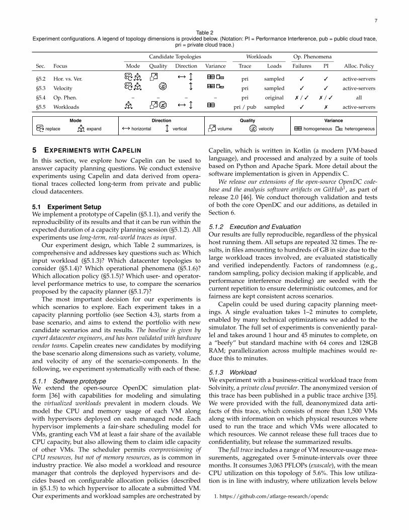
0.0 0.2 0.4 0.6 0.8 1.0 1.2

Overcomm. CPU Cycles [MFLOP] ×1010

replay

active-servers

active-servers(calibrated)

Allo

catio

n Po

licy

Topologybase

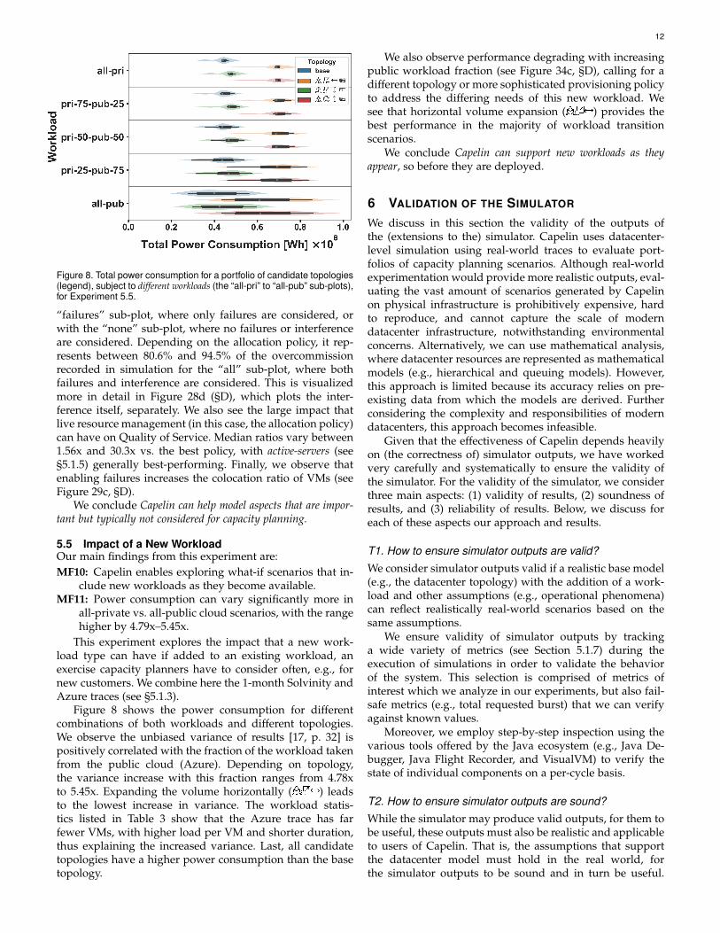
Figure 9. Validation with a replay policy, copying the exact cluster as-signment of the original deployment. For a legend of topologies, seeTable 2.

Concretely, a particular choice of scheduling policy mightproduce valid results, yet may not reflect reality.

To address this, we have created “replay experiments”that replicate the resource management decisions made bythe original infrastructure of the traces, based on placementdata from that time. We do not support live migration ofVMs that occurs in the placement data, since VM placementsare currently fixed over time in OpenDC. However, themajority of VMs do not migrate at all. Capacity issues dueto not supporting live migration are resolved by schedulingVMs on other hosts in the cluster based on the mem policy.

The “replay experiments” are run in an identical setupto the experiments in Section 5 and its results are comparedto the active-servers allocation policy. We visualizeboth raw results and calibrated results, obtained throughonly linear transformations (shifting and scaling values) toaccount for possible constant discrepancy factors. We findthat:

1) The total overcommitted burst shows distributionsthat are similar in shape but differ in scale, forboth policies. This can be explained by the fact thatactive-servers policy is not as effective as themanual placements on the original infrastructure inaddition to the influence of performance interference(Figure 9).

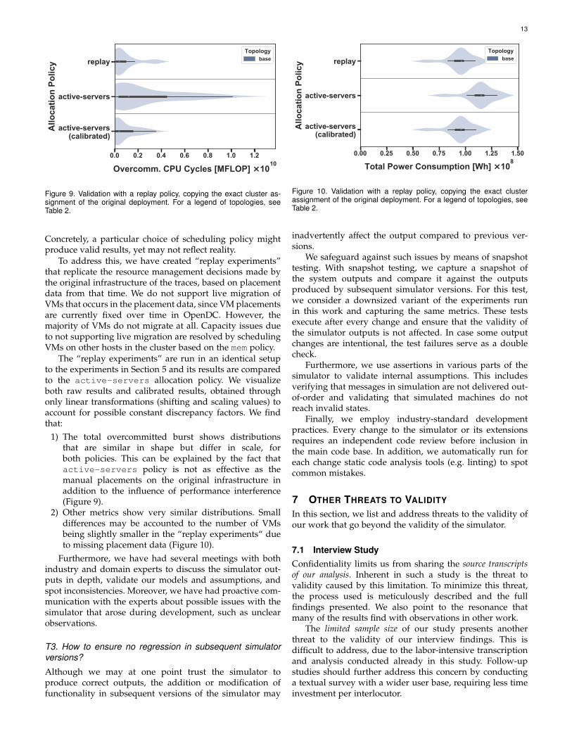
2) Other metrics show very similar distributions. Smalldifferences may be accounted to the number of VMsbeing slightly smaller in the “replay experiments“ dueto missing placement data (Figure 10).

Furthermore, we have had several meetings with bothindustry and domain experts to discuss the simulator out-puts in depth, validate our models and assumptions, andspot inconsistencies. Moreover, we have had proactive com-munication with the experts about possible issues with thesimulator that arose during development, such as unclearobservations.

T3. How to ensure no regression in subsequent simulatorversions?

Although we may at one point trust the simulator toproduce correct outputs, the addition or modification offunctionality in subsequent versions of the simulator may

0.00 0.25 0.50 0.75 1.00 1.25 1.50

Total Power Consumption [Wh] ×108

replay

active-servers

active-servers(calibrated)

Allo

catio

n Po

licy

Topologybase

Figure 10. Validation with a replay policy, copying the exact clusterassignment of the original deployment. For a legend of topologies, seeTable 2.

inadvertently affect the output compared to previous ver-sions.

We safeguard against such issues by means of snapshottesting. With snapshot testing, we capture a snapshot ofthe system outputs and compare it against the outputsproduced by subsequent simulator versions. For this test,we consider a downsized variant of the experiments runin this work and capturing the same metrics. These testsexecute after every change and ensure that the validity ofthe simulator outputs is not affected. In case some outputchanges are intentional, the test failures serve as a doublecheck.

Furthermore, we use assertions in various parts of thesimulator to validate internal assumptions. This includesverifying that messages in simulation are not delivered out-of-order and validating that simulated machines do notreach invalid states.

Finally, we employ industry-standard developmentpractices. Every change to the simulator or its extensionsrequires an independent code review before inclusion inthe main code base. In addition, we automatically run foreach change static code analysis tools (e.g. linting) to spotcommon mistakes.

7 OTHER THREATS TO VALIDITY

In this section, we list and address threats to the validity ofour work that go beyond the validity of the simulator.

7.1 Interview StudyConfidentiality limits us from sharing the source transcriptsof our analysis. Inherent in such a study is the threat tovalidity caused by this limitation. To minimize this threat,the process used is meticulously described and the fullfindings presented. We also point to the resonance thatmany of the results find with observations in other work.

The limited sample size of our study presents anotherthreat to the validity of our interview findings. This isdifficult to address, due to the labor-intensive transcriptionand analysis conducted already in this study. Follow-upstudies should further address this concern by conductinga textual survey with a wider user base, requiring less timeinvestment per interlocutor.

14

7.2 Experimental Study

We discuss three threats related to the experimental study.

7.2.1 Diversity of Modeled Resources

Building topologies in practice requires consideration ofmany different kinds of resources. In our study, we onlyactively explore the CPU resource dimension in the capacityplanning process, to restrict the scope. This could be seenAdding or removing CPUs to/from a machine however canrelate to different types of memory or network becomingapplicable or necessary. This can have impacts on costs andenergy consumption, altering the decision support providedin this study. Nevertheless, the performance should sufferonly minimal impact from this, since CPU consumption canbe regarded as the critical factor in these considerations. Inaddition, Capelin and it’s core abstraction of portfolios ofscenarios offers a broader framework and future extensionsto OpenDC will directly become available to planners usingCapelin.

7.2.2 Public Data Artifacts

A second threat to validity could be perceived in the ab-sence of public experiment data artifacts. The confidentialityof the trace and topology we use in simulation prohibitsthe release of detailed artifacts and results. However, ananonymized version of the trace is available in a public tracearchive, which can be used to explore a restricted set of theworkload. The Azure traces used in the experiment in §5.5are public, along with our sampling logic for their use, andcan therefore be locally used along with the codebase.

Last, a threat to validity could be seen in the validity ofthe outputs of the (extensions to the) simulator itself. We coverthis threat extensively in Section 6.

7.2.3 Allocation Policies

We discuss in this section the relevance of the chosen alloca-tion policies in this work and how they relate to allocationpolicies used in popular resource management tools such asOpenStack, Kubernetes, and VMWare vSphere.

The allocation policies used in this work use a rankingmechanism which orders candidate hosts based on somecriterion (e.g., available memory or number of active VMs)and selects either the lowest or highest ranking host.

OpenStack uses by default the Filter Scheduler2 forplacement of VMs onto hosts. For this, it uses a two stepprocess, consisting of filtering and weighing. During the filter-ing phase, the scheduler filters the available hosts based ona set of user-configured policies (e.g., based on the numberof available vCPUs). In the weighing phase, the scheduleruses a selection of policies to assign weights to the hoststhat survived the filtering phase, and select the host withthe highest weight. How the weights are determined canbe configured by the user, but by default the schedulerwill spread VMs across all hosts evenly based the availableRAM3, similar to the available-mem policy in this work.

2. https://docs.openstack.org/nova/latest/user/filter-scheduler.html

3. https://docs.openstack.org/nova/latest/admin/configuration/schedulers.html#id18

Kubernetes conceptually uses almost exactly the sameprocess as OpenStack4, but by default uses more extensiveweighing policies to ensure the workloads are balanced overthe hosts, also taking into account dynamic informationsuch as resource utilization. A key difference with Open-Stack is that Kubernetes does not consider the memoryrequirements of workloads when weighing the hosts.

VMWare vSphere offers DRS (Distributed ResourceScheduler) which automatically balances workloads acrosshosts in a cluster based on memory requirements of theworkloads.

8 RELATED WORK

We summarize in this section the most closely related work,which we identified through a survey of the field thatyielded over 75 relevant references. Overall, our work isthe first to: (1) conduct community interviews with capac-ity planning practitioners managing cloud infrastructures,which resulted in unique insights and requirements, (2)design and evaluate a data-driven, comprehensive approachto cloud capacity planning, which models real-world op-erational phenomena and provides, through simulation,multiple VM-level metrics as support to capacity planningdecisions.

8.1 Community InterviewsRelated to (1), we see two works as closely related to ourinterview study of practitioners. In the late-1980s, Lam andChan conducted a written questionnaire survey [44] and,mid-2010s, Bauer and Bellamy conducted semi-structuredinterviews [6]. The target group of these studies differsfrom ours, however, since both focus on practitioners fromdifferent industries planning the resources used by their ITdepartment. We summarize both related works below.

Lam and Chan (1987) conduct a written survey with388 participants [44, p. 142]. The survey consists of scaledquestions where practitioners indicate how frequently theyuse certain strategies in different stages of the capacityplanning process [44, p. 143]. Their results indicate thatvery few respondents believe that they use “sophisticated”forecasting techniques for their capacity planning activities,with visual trending being the most popular strategy atthat time. They find that “many companies still rely onthe simplistic, rules-of-thumb, or judgmental approach” tocapacity planning [44, p. 8]. More importantly even, theauthors believe that there is a “significant gap betweentheory and practice as to the usability of the scientific andthe more sophisticated techniques”. The conclusions Lamand Chan draw from their survey and the relations weobserve in their results are resonant with the findings of ourstudy. This stresses the need for a usable and comprehensivecapacity planning system for today’s computer systems.

Bauer and Bellamy (2017) conduct 12 in-person inter-views with “IT capacity-management practitioners” [6] insix different industries. Similar to our interviewing style,the interviews were “semi-structured”, guided by questionsprepared in advance. The questions range from capacity

4. https://kubernetes.io/docs/concepts/scheduling-eviction/kube-scheduler/#kube-scheduler-implementation

15

planning process questions to more managerial questionsaround organizational structure. After manual evaluation ofthe interview transcripts, the authors find that practitionersoften state that the number of capacity planning roles inorganizations is decreasing, while the discipline is still verymuch relevant. The practitioners also find that “vendor-relationship management and contract management” areplaying an increasing role in the capacity planning pro-cess, as well as redundancy and multi-cloud considerations.These results, even if for a different target group, resonatewith our findings in two ways: (1) they underline our callfor the need to focus on the capacity planning process asan essential part of resource management, and (2) empha-size the multi-disciplinary, complex nature of the decisionsneeding to be taken.

8.2 Capacity Planning ApproachesRelated to (2), our work extends the body of related workin three key areas: (1) process models for capacity planning,(2) works related to capacity planning, and (3) system-levelsimulators.

8.2.1 Process Models for Capacity PlanningFirstly, we survey process models for capacity planningpublished in literature. To enable their comparison, we unifythe terminology and the stages proposed by these models,and create the super-set of systems-related stages summa-rized in Table 5. We observe that the first stages (assessmentand characterization) have the broadest support amongmodels. However, we also find significant differences inthe comprehensiveness of models. We observe that the laterstages (deployment and calibration) tend to receive moreattention only in more recent publications. From a systemsperspective, Capelin proposes the first comprehensive pro-cess.

8.2.2 Works Related to Capacity PlanningSecondly, we survey systematically the main scientificrepositories and collect 56 works related to capacity plan-ning. While we plan to release the full survey at a laterstage, we share key insights here. We find that the majorityof studies only consider one resource dimension, and fourinputs or less for their capacity planning model. Few aresimulation-based [1, 13, 48, 51, 52, 53], with the rest usingprimarily analytical models. We highlight three of theseworks below and position them in relation to this work.

Rolia et al. proposes the first trace-based approach tothe problem [53]. Their “Quartermaster” capacity managerservice motivates the use of what-if questions to optimizeSLOs, with the help of trace-based analysis and optimizingsearch for optimal capacity plan suggestions. It’s underlyingsimulation is restricted to replay with no additional mod-elling of phenomena or policies. This severely limits thescope and coverage of the exploration, regarding only onedimension (quantity of CPUs). The work also does not for-mally specify what-if scenarios, even though mentioning thewide variety of scenarios (questions) that can be formulated.

Carvalho et al. uses queuing-theory models to optimizethe computational capacity of datacenters [13]. Their modelsare built from high-level workload characteristics derived

Table 5Comparison of process models for capacity planning. Sources: Lam

and Chan [44, p. 92], Howard [33] (referenced by Browning [11, p. 7]),Menasce and Almeida [47, p. 179], Gunther [27, p. 22], and Kejariwal

and Allspaw [40, p. 4].

Stage [44] [11] [47] [27] [40] Capelin

Assessing current cap. X X X X XIdentifying all workloads X XCharacterize workloads X X X X XAggregate workloads X XValidate workload char. X XDetermine resource req. X XPredict workload X X X XCharacterize perf. X X XValidate perf. char. X X XPredict perf. X X XCharacterize cost X XPredict cost X XAnalyze cost and perf. X XExamine what-if scen. X XDesign system X XIterate and calibrate X X

from traces and include admission control policies. Thesimplifying assumptions made in constructing these simula-tion models restrict the realism of their output. In addition,while this work emphasizes the role that trade-offs play inthe decision-making process, the trade-offs themselves areonly evaluated on a single-metric scale (combining multiplemetrics into one), leaving practitioners with a single outputplan to accept or reject.

The notable Janus [1] presents a real-time risk-basedplanning approach for datacenter networks. The scope ofthis study differs from our scope, in that it addresses net-works and aims to assist in real-time, operational changes.However, we share a focus on operational risks and in-volved costs, and Janus also is evaluated with the help ofreal-world traces.

Our scope of long-term planning (procurement) ex-cludes more dynamic, short-term process such as Google’sAuxon [32] or the Cloud Capacity Manager [41], whichaddress the live management of capacity already procured;explained differently, Capelin (this work) helps decide onlong-term capacity procurement, whereas Auxon and otherslike focus on the different problems of what to do withthat capacity, short-term, once it is already there. Otherwork investigates the dynamic management of physicalcomponents, such as CPU frequency scaling [45].

8.2.3 System-Level Simulators

Thirdly, we survey system-level simulators, and study 10of the best-known in the large-scale distributed systemscommunity. Among the simulators that support VMs al-ready [12, 31, 50] and could thus be useful for simulatingcloud datacenters, few have been tested with traces at thescale of this study, few support CPU overcommissioning,none supports both operational phenomena used in thiswork, and none can output detailed VM-level metrics.

9 CONCLUSION AND FUTURE WORK

Accurately planning cloud datacenter capacity is key tomeeting the needs of the 2020s society whilst saving costs

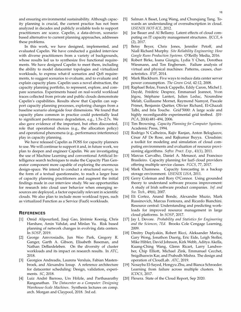
16

and ensuring environmental sustainability. Although capac-ity planning is crucial, the current practice has not beenanalyzed in decades and publicly available tools to supportpractitioners are scarce. Capelin, a data-driven, scenario-based alternative to current planning approaches, addressesthese problems.

In this work, we have designed, implemented, andevaluated Capelin. We have conducted a guided interviewwith diverse practitioners from a variety of backgrounds,whose results led us to synthesize five functional require-ments. We have designed Capelin to meet them, includingthe ability to model datacenter topologies and virtualizedworkloads, to express what-if scenarios and QoS require-ments, to suggest scenarios to evaluate, and to evaluate andexplain capacity plans. Capelin uses a novel abstraction, thecapacity planning portfolio, to represent, explore, and com-pare scenarios. Experiments based on real-world workloadtraces collected from private and public clouds demonstrateCapelin’s capabilities. Results show that Capelin can sup-port capacity planning processes, exploring changes from abaseline scenario alongside four dimensions. We found thatcapacity plans common in practice could potentially leadto significant performance degradation, e.g., 1.5x–2.7x. Wealso gave evidence of the important, but often discounted,role that operational choices (e.g., the allocation policy)and operational phenomena (e.g., performance interference)play in capacity planning.

We have released Capelin as FOSS for capacity plannersto use. We will continue to support it and, in future work, weplan to deepen and engineer Capelin. We are investigatingthe use of Machine Learning and conventional Artificial In-telligence search techniques to make the Capacity Plan Gen-erator component more capable of exploring the enormousdesign-space. We intend to conduct a structured survey, inthe form of a textual questionnaire, to reach a larger baseof capacity planning practitioners and augment the initialfindings made in our interview study. We see opportunitiesfor research into cloud user behavior when emerging re-sources are deployed, a factor especially relevant in scientificclouds. We also plan to include more workload types, suchas virtualized Function as a Service (FaaS) workloads.

REFERENCES

[1] Omid Alipourfard, Jiaqi Gao, Jeremie Koenig, ChrisHarshaw, Amin Vahdat, and Minlan Yu. Risk basedplanning of network changes in evolving data centers.In SOSP, 2019.

[2] George Amvrosiadis, Jun Woo Park, Gregory R.Ganger, Garth A. Gibson, Elisabeth Baseman, andNathan DeBardeleben. On the diversity of clusterworkloads and its impact on research results. In ATC,2018.

[3] Georgios Andreadis, Laurens Versluis, Fabian Masten-broek, and Alexandru Iosup. A reference architecturefor datacenter scheduling: Design, validation, experi-ments. SC, 2018.

[4] Luiz Andre Barroso, Urs Holzle, and ParthasarathyRanganathan. The Datacenter as a Computer: DesigningWarehouse-Scale Machines. Synthesis lectures on comp.arch. Morgan and Claypool, 2018. 3rd ed.

[5] Salman A Baset, Long Wang, and Chunqiang Tang. To-wards an understanding of oversubscription in cloud.USENIX HOT-ICE, 2012.

[6] Joe Bauer and Al Bellamy. Latent effects of cloud com-puting on IT capacity management structures. IJCCE, 6(2), 2017.

[7] Betsy Beyer, Chris Jones, Jennifer Petoff, andNiall Richard Murphy. Site Reliability Engineering: HowGoogle Runs Production Systems. O’Reilly Media, 2016.

[8] Robert Birke, Ioana Giurgiu, Lydia Y Chen, DorotheaWiesmann, and Ton Engbersen. Failure analysis ofvirtual and physical machines: Patterns, causes, char-acteristics. IFIP, 2014.

[9] Mark Blackburn. Five ways to reduce data center serverpower consumption. The Green Grid, 42:12, 2008.

[10] Raphael Bolze, Franck Cappello, Eddy Caron, Michel J.Dayde, Frederic Desprez, Emmanuel Jeannot, YvonJegou, Stephane Lanteri, Julien Leduc, NouredineMelab, Guillaume Mornet, Raymond Namyst, PascalePrimet, Benjamin Quetier, Olivier Richard, El-GhazaliTalbi, and Irea Touche. Grid’5000: A large scale andhighly reconfigurable experimental grid testbed. IJH-PCA, 20(4):481–494, 2006.

[11] Tim Browning. Capacity Planning for Computer Systems.Academic Press, 1994.

[12] Rodrigo N Calheiros, Rajiv Ranjan, Anton Beloglazov,Cesar AF De Rose, and Rajkumar Buyya. Cloudsim:a toolkit for modeling and simulation of cloud com-puting environments and evaluation of resource provi-sioning algorithms. Softw. Pract. Exp., 41(1), 2011.

[13] Marcus Carvalho, Daniel A. Menasce, and FranciscoBrasileiro. Capacity planning for IaaS cloud providersoffering multiple service classes. FGCS, 77, 2017.

[14] Mark Chamness. Capacity forecasting in a backupstorage environment. USENIX LISA, 2011.

[15] Gerry Coleman and Rory O’Connor. Using groundedtheory to understand software process improvement:A study of Irish software product companies. Inf. andSw. Tech., 49(6), 2007.

[16] Eli Cortez, Anand Bonde, Alexandre Muzio, MarkRussinovich, Marcus Fontoura, and Ricardo Bianchini.Resource central: Understanding and predicting work-loads for improved resource management in largecloud platforms. In SOSP, 2017.

[17] Jay L Devore. Probability and Statistics for Engineeringand the Sciences, 7Ed. Brooks Cole Cengage Learning,2009.

[18] Dmitry Duplyakin, Robert Ricci, Aleksander Maricq,Gary Wong, Jonathon Duerig, Eric Eide, Leigh Stoller,Mike Hibler, David Johnson, Kirk Webb, Aditya Akella,Kuang-Ching Wang, Glenn Ricart, Larry Landwe-ber, Chip Elliott, Michael Zink, Emmanuel Cecchet,Snigdhaswin Kar, and Prabodh Mishra. The design andoperation of CloudLab. ATC, 2019.

[19] Nosayba El-Sayed, Hongyu Zhu, and Bianca Schroeder.Learning from failure across multiple clusters. InICDCS, 2017.

[20] Flexera. State of the Cloud Report, Sep 2020.

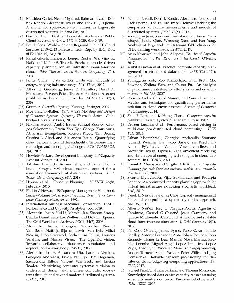
17

[21] Matthieu Gallet, Nezih Yigitbasi, Bahman Javadi, Der-rick Kondo, Alexandru Iosup, and Dick H. J. Epema.A model for space-correlated failures in large-scaledistributed systems. In Euro-Par, 2010.

[22] Gartner Inc. Gartner Forecasts Worldwide PublicCloud Revenue to Grow 17% in 2020, Sep 2019.

[23] Frank Gens. Worldwide and Regional Public IT CloudServices 2019–2023 Forecast. Tech. Rep. by IDC, Doc.#US44202119, Aug 2019.

[24] Rahul Ghosh, Francesco Longo, Ruofan Xia, Vijay K.Naik, and Kishor S. Trivedi. Stochastic model drivencapacity planning for an infrastructure-as-a-servicecloud. IEEE Transactions on Services Computing, 7(4),2014.

[25] James Glanz. Data centers waste vast amounts ofenergy, belying industry image. N.Y. Times, 2012.

[26] Albert G. Greenberg, James R. Hamilton, David A.Maltz, and Parveen Patel. The cost of a cloud: researchproblems in data center networks. ACM CCR, 39(1),2009.

[27] Gunther. Guerrilla Capacity Planning. Springer, 2007.[28] Mor Harchol-Balter. Performance Modeling and Design

of Computer Systems: Queueing Theory in Action. Cam-bridge University Press, 2013.

[29] Nikolas Herbst, Andre Bauer, Samuel Kounev, Gior-gos Oikonomou, Erwin Van Eyk, George Kousiouris,Athanasia Evangelinou, Rouven Krebs, Tim Brecht,Cristina L. Abad, and Alexandru Iosup. Quantifyingcloud performance and dependability: Taxonomy, met-ric design, and emerging challenges. ACM TOMPECS,3(4), 2018.

[30] Hewlett-Packard Development Company. HP CapacityAdvisor Version 7.4, 2014.

[31] Takahiro Hirofuchi, Adrien Lebre, and Laurent Pouil-loux. Simgrid VM: virtual machine support for asimulation framework of distributed systems. IEEETrans. Cloud Computing, 6(1), 2018.

[32] Hixson et al. Capacity Planning. USENIX ;login,February, 2015.

[33] Phillip C Howard. IS Capacity Management HandbookSeries–Volume 1–Capacity Planning. Institute for Com-puter Capacity Management, 1992.

[34] International Business Machines Corporation. IBM ZPerformance and Capacity Analytics tool, 2019.

[35] Alexandru Iosup, Hui Li, Mathieu Jan, Shanny Anoep,Catalin Dumitrescu, Lex Wolters, and Dick H J Epema.The Grid Workloads Archive. FGCS, 24(7), 2008.

[36] Alexandru Iosup, Georgios Andreadis, VincentVan Beek, Matthijs Bijman, Erwin Van Eyk, MihaiNeacsu, Leon Overweel, Sacheendra Talluri, LaurensVersluis, and Maaike Visser. The OpenDC vision:Towards collaborative datacenter simulation andexploration for everybody. ISPDC, 2017.

[37] Alexandru Iosup, Alexandru Uta, Laurens Versluis,Georgios Andreadis, Erwin Van Eyk, Tim Hegeman,Sacheendra Talluri, Vincent Van Beek, and LucianToader. Massivizing computer systems: A vision tounderstand, design, and engineer computer ecosys-tems through and beyond modern distributed systems.ICDCS, 2018.

[38] Bahman Javadi, Derrick Kondo, Alexandru Iosup, andDick Epema. The Failure Trace Archive: Enabling thecomparison of failure measurements and models ofdistributed systems. JPDC, 73(8), 2013.

[39] Myeongjae Jeon, Shivaram Venkataraman, Amar Phan-ishayee, Junjie Qian, Wencong Xiao, and Fan Yang.Analysis of large-scale multi-tenant GPU clusters forDNN training workloads. In ATC, 2019.

[40] Arun Kejariwal and John Allspaw. The Art of CapacityPlanning: Scaling Web Resources in the Cloud. O’Reilly,2017.

[41] Mukil Kesavan et al. Practical compute capacity man-agement for virtualized datacenters. IEEE TCC, 1(1):1–1, 2013.

[42] Younggyun Koh, Rob Knauerhase, Paul Brett, MicBowman, Zhihua Wen, and Calton Pu. An analysisof performance interference effects in virtual environ-ments. In ISPASS, 2007.

[43] Rouven Krebs, Christof Momm, and Samuel Kounev.Metrics and techniques for quantifying performanceisolation in cloud environments. Science of ComputerProgramming, 2014.

[44] Shui F Lam and K Hung Chan. Computer capacityplanning: theory and practice. Academic Press, 1987.

[45] Drazen Lucanin et al. Performance-based pricing inmulti-core geo-distributed cloud computing. IEEETCC, 2016.

[46] Fabian Mastenbroek, Georgios Andreadis, SoufianeJounaid, Wenchen Lai, Jacob Burley, Jaro Bosch, Er-win van Eyk, Laurens Versluis, Vincent van Beek, andAlexandru Iosup. OpenDC 2.0: Convenient modelingand simulation of emerging technologies in cloud dat-acenters. In CCGRID, 2021.

[47] Daniel A. Menasce and Virgılio A.F. Almeida. CapacityPlanning for Web Services: metrics, models, and methods.Prentice Hall, 2001.

[48] Swarna Mylavarapu, Vijay Sukthankar, and PradiptaBanerjee. An optimized capacity planning approach forvirtual infrastructure exhibiting stochastic workload.SAC, 2010.

[49] Derek L. Nazareth and Jae Choi. Capacity managementfor cloud computing: a system dynamics approach.AMCIS, 2017.

[50] Alberto Nunez, Jose L Vazquez-Poletti, Agustin CCaminero, Gabriel G Castane, Jesus Carretero, andIgnacio M Llorente. iCanCloud: A flexible and scalablecloud infrastructure simulator. J. Grid Comput., 10(1),2012.

[51] Per Olov Ostberg, James Byrne, Paolo Casari, PhilipEardley, Antonio Fernandez Anta, Johan Forsman, JohnKennedy, Thang Le Duc, Manuel Noya Marino, Rad-hika Loomba, Miguel Angel Lopez Pena, Jose LopezVeiga, Theo Lynn, Vincenzo Mancuso, Sergej Svorobej,Anders Torneus, Stefan Wesner, Peter Willis, and JorgDomaschka. Reliable capacity provisioning for dis-tributed cloud/edge/fog computing applications. Eu-CNC, 2017.

[52] Jayneel Patel, Shahram Sarkani, and Thomas Mazzuchi.Knowledge based data center capacity reduction usingsensitivity analysis on causal Bayesian belief network.IKSM, 12(2), 2013.

18

[53] Jerry Rolia, Ludmila Cherkasova, Martin Arlitt, andArtur Andrzejak. A capacity management service forresource pools. WOSP, 2005.

[54] Semih Salihoglu and M Tamer Ozsu. Response to ”scaleup or scale out for graph processing”. IEEE InternetComput., 22(5), 2018.

[55] Siqi Shen, Vincent Van Beek, and Alexandru Iosup. Sta-tistical characterization of business-critical workloadshosted in cloud datacenters. CCGrid, 2015.

[56] Zhiming Shen, Sethuraman Subbiah, Xiaohui Gu, andJohn Wilkes. CloudScale: Elastic resource scaling formulti-tenant cloud systems. SoCC, 2011.

[57] Ling Tang and Hao Chen. Joint pricing and capacityplanning in the IaaS cloud market. IEEE TCC, 5(1),2017.

[58] Daniel W Turner. Qualitative Interview Design: APractical Guide for Novice Investigators. QualitativeReport, 15(3):7, 2010.

[59] Vincent van Beek, Jesse Donkervliet, Tim Hegeman,Stefan Hugtenburg, and Alexandru Iosup. Self-Expressive Management of Business-Critical Work-loads in Virtualized Datacenters. Computer, 48(7):46–54,2015.

[60] Vincent van Beek, Giorgos Oikonomou, and AlexandruIosup. A CPU contention predictor for business-criticalworkloads in cloud datacenters. In HotCloudPerf, 2019.

[61] Arunchandar Vasan, Anand Sivasubramaniam, VikrantShimpi, T. Sivabalan, and Rajesh Subbiah. Worththeir watts? - an empirical study of datacenter servers.HPCA, 2010.

[62] VMware. VMware Capacity Planner, 2009.[63] Jie Xu and Chenbo Zhu. Optimal pricing and capacity

planning of a new economy cloud computing serviceclass. ICCAC, 2015.

[64] Ennan Zhai, Ruzica Piskac, Ronghui Gu, Xun Lao,and Xi Wang. An auditing language for preventingcorrelated failures in the cloud. PACMPL, 2017.

[65] Chun Zhang, Rong N. Chang, Chang Shing Perng, Ed-ward So, Chungqiang Tang, and Tao Tao. An optimalcapacity planning algorithm for provisioning cluster-based failure-resilient composite services. SCC, 2009.

[66] Qi Zhang, Ludmila Cherkasova, Guy Mathews, WayneGreene, and Evgenia Smirni. R-capriccio: A capacityplanning and anomaly detection tool for enterpriseservices with live workloads. Middleware, 2007.

APPENDIX ACAPACITY PLANNING INTERVIEW SCRIPT

In this chapter, we list the interview script used for theinterviews described in Section 3. To encode instructionsto the reviewer, we use the following notation. The fontdetermines the type of instruction: Questions are writtenin standard fonts, emphasis indicates instructions to be readto the interlocutor by the interviewer (not necessarily ver-batim), and mono-space font represents instructions for thereviewer. The questions are numbered for cross-referenceand divided into 5 category. Each question is assigned oneout of three priority levels, indicated by asterisks (*, **,and ***), with three stars indicating the highest priority.Each category (section) of questions is allocated a numberof minutes, listed between parentheses.

A.1 Part 1: Overview (15’)Thanks for agreeing to meet with me. To get the most out of thisconversation, would you allow me to record the conversation fornote-taking purposes? I will not share the recording with anyoneelse but you, if you want a copy, and I will delete the recording atthe end of my thesis project.

If you have any concerns about sharing this kind of informa-tion with me, let us talk quickly and openly about it. We hope youwill share openly. Rest assured, we want more to learn about theissues around capacity planning than to publish on it.

I will transcribe the recording for myself, and for any use of asnippet of your words, I will ask you specifically for approval torelease, with due reference, unless you want me to keep the authoranonymous, of course.

We are interested in learning more about how businessesthink about having IT infrastructure and services always availableand plentiful. We call this capacity planning, and know we arereferring here only to IT and the IT team, and not to other types of“capacity”. We want to learn and share with you what processesare used, what challenges exist, and how can we help solve them.(Q1) *** How important is it to have IT infrastructure

and services always available and plentiful inyour business?

(Q2) *** What kind of services do you provide? Howimportant is it for your different services?

(Q3) *** Can you give us an example of a success incapacity planning? Share with us a good idea,a good process, some situation when all workedwell?

(Q4) *** Can you give us an example of an insuccess incapacity planning? Share with us a mistake, anerroneous process, some situation when manythings failed to worked well or took much moreto get through than expected?

(Q5) *** What does the typical process for capacity plan-ning look like at your company? You can startwith an overview, or even from a concrete exam-ple, like how to get a new cluster in operation.

(Q6) ** A few yes or no questions:1) Do you have “what if” scenarios?2) Do you consider hybrid or public clouds to be

part of your capacity planning process?3) Would you be willing to share historical data

on capacity planning?

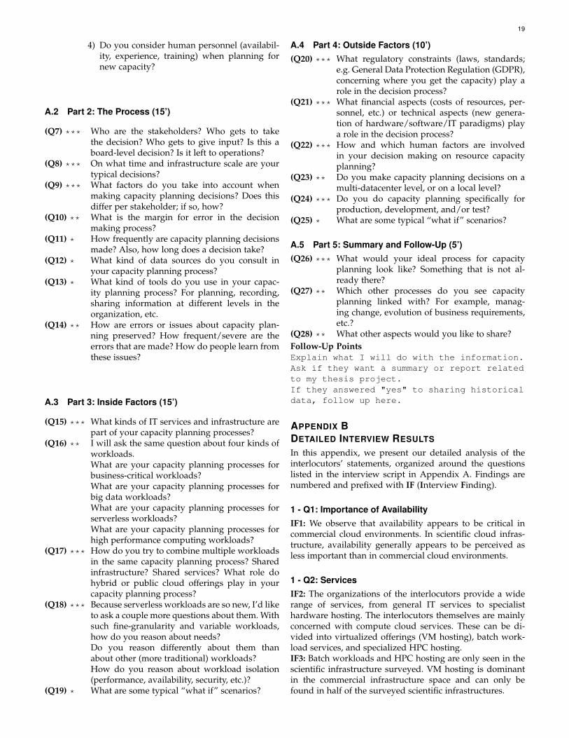
19

4) Do you consider human personnel (availabil-ity, experience, training) when planning fornew capacity?

A.2 Part 2: The Process (15’)

(Q7) *** Who are the stakeholders? Who gets to takethe decision? Who gets to give input? Is this aboard-level decision? Is it left to operations?

(Q8) *** On what time and infrastructure scale are yourtypical decisions?

(Q9) *** What factors do you take into account whenmaking capacity planning decisions? Does thisdiffer per stakeholder; if so, how?

(Q10) ** What is the margin for error in the decisionmaking process?

(Q11) * How frequently are capacity planning decisionsmade? Also, how long does a decision take?

(Q12) * What kind of data sources do you consult inyour capacity planning process?

(Q13) * What kind of tools do you use in your capac-ity planning process? For planning, recording,sharing information at different levels in theorganization, etc.

(Q14) ** How are errors or issues about capacity plan-ning preserved? How frequent/severe are theerrors that are made? How do people learn fromthese issues?

A.3 Part 3: Inside Factors (15’)

(Q15) *** What kinds of IT services and infrastructure arepart of your capacity planning processes?

(Q16) ** I will ask the same question about four kinds ofworkloads.What are your capacity planning processes forbusiness-critical workloads?What are your capacity planning processes forbig data workloads?What are your capacity planning processes forserverless workloads?What are your capacity planning processes forhigh performance computing workloads?

(Q17) *** How do you try to combine multiple workloadsin the same capacity planning process? Sharedinfrastructure? Shared services? What role dohybrid or public cloud offerings play in yourcapacity planning process?

(Q18) *** Because serverless workloads are so new, I’d liketo ask a couple more questions about them. Withsuch fine-granularity and variable workloads,how do you reason about needs?Do you reason differently about them thanabout other (more traditional) workloads?How do you reason about workload isolation(performance, availability, security, etc.)?

(Q19) * What are some typical “what if” scenarios?

A.4 Part 4: Outside Factors (10’)(Q20) *** What regulatory constraints (laws, standards;

e.g. General Data Protection Regulation (GDPR),concerning where you get the capacity) play arole in the decision process?

(Q21) *** What financial aspects (costs of resources, per-sonnel, etc.) or technical aspects (new genera-tion of hardware/software/IT paradigms) playa role in the decision process?

(Q22) *** How and which human factors are involvedin your decision making on resource capacityplanning?

(Q23) ** Do you make capacity planning decisions on amulti-datacenter level, or on a local level?

(Q24) *** Do you do capacity planning specifically forproduction, development, and/or test?

(Q25) * What are some typical “what if” scenarios?

A.5 Part 5: Summary and Follow-Up (5’)(Q26) *** What would your ideal process for capacity

planning look like? Something that is not al-ready there?

(Q27) ** Which other processes do you see capacityplanning linked with? For example, manag-ing change, evolution of business requirements,etc.?

(Q28) ** What other aspects would you like to share?Follow-Up PointsExplain what I will do with the information.Ask if they want a summary or report relatedto my thesis project.If they answered "yes" to sharing historicaldata, follow up here.

APPENDIX BDETAILED INTERVIEW RESULTS

In this appendix, we present our detailed analysis of theinterlocutors’ statements, organized around the questionslisted in the interview script in Appendix A. Findings arenumbered and prefixed with IF (Interview Finding).

1 - Q1: Importance of AvailabilityIF1: We observe that availability appears to be critical incommercial cloud environments. In scientific cloud infras-tructure, availability generally appears to be perceived asless important than in commercial cloud environments.

1 - Q2: ServicesIF2: The organizations of the interlocutors provide a widerange of services, from general IT services to specialisthardware hosting. The interlocutors themselves are mainlyconcerned with compute cloud services. These can be di-vided into virtualized offerings (VM hosting), batch work-load services, and specialized HPC hosting.IF3: Batch workloads and HPC hosting are only seen in thescientific infrastructure surveyed. VM hosting is dominantin the commercial infrastructure space and can only befound in half of the surveyed scientific infrastructures.

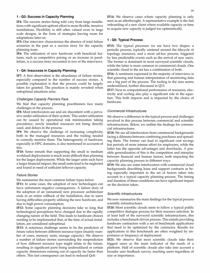
20

1 - Q3: Success in Capacity PlanningIF4: The success stories being told vary from large installa-tions with significant upfront effort to more flexible, iterativeinstallations. Flexibility is still often valued even in largescale designs, in the form of strategies leaving room foradaptations later-on.IF5: One interview characterizes the absence of total failurescenarios in the past as a success story for the capacityplanning team.IF6: The utilization of new hardware with beneficial fea-tures, such as competitive pricing or an increase in paral-lelism, is a success story recounted in two of the interviews.

1 - Q4: Insuccess in Capacity PlanningIF7: A first observation is the abundance of failure stories,especially compared to the number of success stories. Apossible explanation is that the process could be largelytaken for granted. The practices is mainly revisited whensuboptimal situations arise.

Challenges Capacity Planners FaceWe find that capacity planning practitioners face manychallenges in the process.IF8: Most interlocutors see and are discontent with a perva-sive under-utilization of their system. This under-utilizationcan be caused by operational risk minimization takingprecedence, newly installed resources not being directlyused, and delays in the process.IF9: We observe the challenge of increasing complexity,both in the managed resources and the tooling neededto correctly monitor them. The heterogeneity of hardware,especially in HPC domains, is also mentioned in accounts ofthis.IF10: Some remark that supporting the small to mediumworkload deployments is much more difficult than planningfor the larger deployments. While the larger units each havea larger financial impact, the small units tend to be neglectedand found in need of sufficient leftover capacity.

Failure StoriesWe summarize the most common failure types below.IF11: In some cases, the adoption of new technologies canhave unforeseen negative consequences. A failure story ofthe adoption of an (unnamed) new processor architectureends in an entire rollback of the installation, due to usershaving difficulties properly utilizing the new hardware, anddue to high power consumption.IF12: Some capacity planning decisions take so long thattechnological perceptions have changed due to the rapidlychanging nature of the field. This leads to hardware choicesneeding to be implemented that, at the time of actual instal-lation, are considered suboptimal.IF13: A notorious challenge seems to be the prediction offuture ratios between different resource types (mainly num-ber of cores, memory units, storage capacity). We observea number of failure stories surrounding the mispredictionof how different resource type might relate in the future,resulting in significant parts being underutilized or certaincapacity dimensions running out of capacity far faster thanothers. This last consequence can lead to reduced QoS.

IF14: We observe cases where capacity planning is onlyseen as an afterthought. A representative example is the fastonboarding of a new client where available capacity or timeto acquire new capacity is judged too optimistically.

1 - Q5: Typical Process

IF15: The typical processes we see have two shapes: aperiodic process, typically centered around the lifecycle oftopology resources, and a more ad-hoc process, triggeredby less predictable events such as the arrival of new users.The former is dominant in most surveyed scientific clouds,while the latter is more common in commercial clouds. Onescientific cloud in the set has a combination of both.IF16: A sentiment expressed in the majority of interviews isthat guessing and human interpretation of monitoring dataare a big part of the process. The tooling in the area seemsunderutilized, further discussed in Q13.IF17: Next to computational performance of resources, elec-tricity and cooling also play a significant role in the equa-tion. This both impacts and is impacted by the choice ofhardware.

Commercial Infrastructures

We observe a difference in the typical process and challengesinvolved in this process between commercial and scientificinfrastructures. Below, we outline the findings for commer-cial infrastructures.IF18: We see all interlocutors from commercial backgroundsfacing a dilemma between combining purchases and spread-ing them. The former can lead to significant cost savingsbut periods of more intense effort for employees, while thelatter has the opposite advantages and drawbacks. A pos-sible generalization of this is the competition and interplaybetween financial and human factors, both impacting thecapacity planning process in different ways.IF19: We also see some interlocutors with commercial cloudbackgrounds describing lease and support contracts as be-ing especially important in the set of factors taken intoaccount in a typical capacity planning process. The timingand duration of these conditions can have significant impacton the decision taken.

Scientific Infrastructures

We now summarize the main findings for the typical processscientific infrastructures.IF20: Most scientific clouds seem to follow a typical publiccompetitive dialogue process for their resource selection. Inat least half of the surveyed scientific infrastructures, thisincludes a benchmark-driven process. This entails providinghardware contractors with a set of benchmark applicationsthat need to be optimized by the contractor. Results forapplications in this benchmark are often weighted by im-portance or frequency of deployment.IF21: We observe that most scientific clouds take theirbiggest users as the main indicator of the needs of aplatform. Half of scientific clouds also take into account abroader user feedback survey, reaching users regardless ofsize or importance.

21

IF22: Almost all scientific cloud interlocutors perceive theirprocess as fundamentally different from the commercialcapacity planning process. The main perceived differenceis the mode of operation, which they believe to be budget-centered rather than demand-centered. These interlocutorsalso consider their budget-centered to have less capacityplanning efforts than commercial efforts. Whether this as-sessment is accurate is difficult to objectively judge, al-though analysis from other questions seems to indicate thatthere are more aspects of “traditional” capacity planning intheir process than commonly perceived.

1 - Q6: Yes/No Questions

IF23: What-if scenarios do not seem to be established prac-tice currently. Some unstructured examples fitting the for-mat (e.g. fail-over scenarios, clients arriving) are mentionedinformally, but not in a structured form.

IF24: Most of the scientific clouds have exploratory projectsrunning where they investigate the possibility of offloadingdemands to a public cloud. This indicates increased interestin hybrid infrastructure offerings.

IF25: A significant portion of interlocutors is willing toshare historical data with the interviewer. This could signalinterest in academia and industry for more research beingconducted in topics surrounding their capacity planningdecision making.

IF26: The majority of interlocutors considers human person-nel in some form in the capacity planning process. This topicis further analysed in Q22.

2 - Q7: Stakeholders

IF27: All processes surveyed seem to have an executiveboard at the head of the process. This board seek out advicefrom experts in the domains relevant to their decision. Thesecan include technical advisors or scientific experts.

IF28: For all surveyed instances, the final decision seemsto be at board level. While the input of domain experts issought out, the final decision is made by the management.

IF29: The interlocutors with commercial background alsohave an engineer in charge of the capacity planning pro-cess, monitoring the current situation and coordinating thelifecycle-based planning process. The process in this casealso includes input from the hardware contract adminis-tration for contracts. Occasionally, the sales department isinvolved, if the decision affects the shaping or pricing ofservices provided to customers.

IF30: In scientific environments, an important part of the setof stakeholders tend to be scientific partners and (govern-mental) funding agencies. Half of the surveyed processeshere also take into account user input through a user ques-tionnaire.

2 - Q8: Time and Infrastructure Scale

IF31: Unlike the frequency or trigger of capacity planningprocesses, the time scale of the decisions made seem to beroughly uniform across interlocutors. We observe that theaging and thus deterioration of hardware is seen as themost important factor here, with a mean of 5 years untilthe next decision for a specific machine/rack. Commercialenvironments seem to tend towards faster replacement (3-5 years), while scientific environments seem to replace lessquickly (4-7 years).IF32: The infrastructure scale of decisions for commercialenvironments tends to be a single rack. Making multi-rackdecisions is desired, due to potential cost savings, but notalways possible.IF33: In scientific environments, the infrastructure scale ofdecisions seems to be larger, with most surveyed infras-tructures working on scales of entire cluster/site iterations.One infrastructure works on a smaller scale, making single-machine or single-rack decisions.

2 - Q9: Factors

IF34: The number of factors is remarkable, with more than25 distinct factors being named in the full set of interviews.IF35: Nevertheless, the factors that span across a majorityof interviews are few. Only three factors are named in morethan half of the interviews: the use of historical monitor-ing data, financial concerns (such as budget size), and thelifetime of hardware. These are followed up by a set of fourfactors mentioned in slightly less than half of the interviews:user demand, new technologies, incoming projects, and thebenchmark performance of different solutions.IF36: We observe a number of factors particular to scien-tific infrastructures but not being mentioned in the com-mercial set. The most important here are the benchmarkperformance of solutions (which is often required by pub-lic competitive acquisition processes) and user demands.One surveyed infrastructure optimizes for throughput here,meaning the number of times the benchmark can be run ina certain time frame.IF37: Similarly, we observe a number of factors unique tocommercial infrastructures. The most prominent are leasecontracts, current offerings that the provider has, and per-sonnel capacities.

2 - Q10: Margin for Error

IF38: The margin for error is difficult to objectively measure,due to the multi-faceted nature of this process. Two mainconsequences of errors are mentioned by interlocutors. First,financial losses can occur due to overestimation of thedemand of a certain resource, such as specific accelerators orstorage capacity, or due to underestimation, as can happen ifthe ratio of resource types is mispredicted. Second, person-nel can come under pressure, due to available capacity beingsmaller than expected, starting a search for spare capacity inany of the managed clusters.

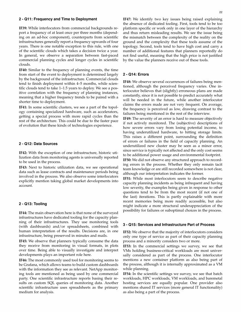
22

2 - Q11: Frequency and Time to Deployment

IF39: While interlocutors from commercial backgrounds re-port a frequency of at least once per three months (depend-ing on an ad-hoc component), counterparts from scientificinfrastructures generally report a frequency upwards of fouryears. There is one notable exception to this rule, with oneof the scientific clouds which takes a decision twice a year.In general, we observe a separation between fast-pacedcommercial planning cycles and longer cycles in scientificclouds.IF40: Similar to the frequency of planning events, the timefrom start of the event to deployment is determined largelyby the background of the infrastructure. Commercial cloudstend to finish deployment within 4–5 months, while scien-tific clouds tend to take 1–1.5 years to deploy. We see a pos-itive correlation with the frequency of planning instances,meaning that a higher frequency trends to be paired with ashorter time to deployment.IF41: In some scientific clusters, we see a part of the topol-ogy containing specialized hardware, such as accelerators,getting a special process with more rapid cycles than therest of the architecture. This could be due to the faster paceof evolution that these kinds of technologies experience.

2 - Q12: Data Sources

IF42: With the exception of one infrastructure, historic uti-lization data from monitoring agents is universally reportedto be used in the process.IF43: Next to historic utilization data, we see operationaldata such as lease contracts and maintenance periods beinginvolved in the process. We also observe some interlocutorsexplicitly mention taking global market developments intoaccount.

2 - Q13: Tooling

IF44: The main observation here is that none of the surveyedinfrastructures have dedicated tooling for the capacity plan-ning of their infrastructures. They use monitoring tools(with dashboards) and/or spreadsheets, combined withhuman interpretation of the results. Decisions are, in oneinfrastructure, being preserved in minutes and mails.IF45: We observe that planners typically consume the datathey receive from monitoring in visual formats, in plotsover time. Being able to visually investigate and interpretdevelopments plays an important role here.IF46: The most commonly used tool for monitoring seems tobe Grafana, which allows teams to build custom dashboardswith the information they see as relevant. NetApp monitor-ing tools are mentioned as being used by one commercialparty. One scientific infrastructure reports basing their re-sults on custom SQL queries of monitoring data. Anotherscientific infrastructure uses spreadsheets as the primarymedium for analysis.

IF47: We identify two key issues being raised explainingthe absence of dedicated tooling. First, tools tend to be tooplatform specific or work only in one layer of the hierarchyand thus return misleading results. We see the issue beingthe mismatch between the complexity of the reality on theground and the complexity that these tools assume of thetopology. Second, tools tend to have high cost and carry anumber of additional features that planners reportedly donot find useful, meaning that the high price is not justifiedby the value the planners receive out of these tools.

2 - Q14: Errors

IF48: We observe several occurrences of failures being men-tioned, although the perceived frequency varies. One in-terlocutor believes that (slightly) erroneous plans are madeconstantly, since it is not possible to predict accurately whatwill be needed in the future, while another interlocutorclaims the errors made are not very frequent. On average,the frequency is perceived as low, drawing contrast to thefailures being mentioned in the rest of the interview.IF49: The severity of an error is hard to measure objectivelyif not actively monitored. The (subjective) descriptions ofhow severe errors vary from losing potential income, tohaving underutilized hardware, to hitting storage limits.This raises a different point, surrounding the definitionof errors or failures in the field of capacity planning. Anunderutilized new cluster may be seen as a minor error,since service is typically not affected and the only cost seemsto be additional power usage and environmental footprint.IF50: We did not observe any structured approach to record-ing errors in the process. Whether they only remain tacitteam knowledge or are still recorded somewhere is not clear,although our interpretation indicates the former.IF51: While most interlocutors seem to describe negativecapacity planning incidents as being infrequent and havinglow severity, the examples being given in response to otherquestions tend to be from the most recent (if not one ofthe last) iterations. This is partly explainable with morerecent memories being more readily accessible, but alsomight indicate a more structural underappreciation of thepossibility for failures or suboptimal choices in the process.

3 - Q15: Services and Infrastructure Part of Process

IF52: We observe that the majority of interlocutors considersonly one type of service as part of their capacity planningprocess and a minority considers two or more.IF53: In the commercial settings we survey, we see thatVMs holding business-critical workloads are most univer-sally considered as part of the process. One interlocutormentions a new container platform as also being part ofthe process, although it is internally approximated as a VMwhile planning.IF54: In the scientific settings we survey, we see that batchworkloads, HPC workloads, VM workloads, and baremetalhosting services are equally popular. One provider alsomentions shared IT services (more general IT functionality)as also being a part of the process.

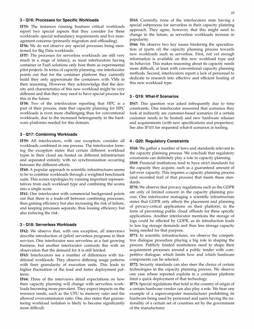
23

3 - Q16: Processes for Specific Workloads

IF55: The instances running business critical workloadsreport two special aspects that they consider for theseworkloads: special redundancy requirements and live man-agement concerns (primarily migration and offloading).IF56: We do not observe any special processes being men-tioned for Big Data workloads.IF57: The processes for serverless workloads are still verymuch in a stage of infancy, as most interlocutors havingcontainer or FaaS solutions only host them as experimentalpilot projects. In terms of capacity planning, one interlocutorpoints out that for the container platform they currentlybuild they only approximate the containers with VMs intheir reasoning. However, they acknowledge that the den-sity and characteristics of this new workload might be verydifferent and that they may need to have special process forthis in the future.IF58: Two of the interlocutors reporting that HPC is apart of their process, state that capacity planning for HPCworkloads is even more challenging than for conventionalworkloads, due to the increased heterogeneity in the hard-ware platforms needed for this domain.

3 - Q17: Combining Workloads

IF59: All interlocutors, with one exception, consider allworkloads combined in one process. The interlocutor form-ing the exception states that certain different workloadtypes in their cloud are hosted on different infrastructureand separated entirely, with no synchronization occurringbetween the different efforts.IF60: A popular approach in scientific infrastructures seemsto be to combine workloads through a weighted benchmarksuite. This scores topologies by running important represen-tatives from each workload type and combining the scoresinto a single score.IF61: One interlocutor with commercial background pointsout that there is a trade-off between combining processes,thus gaining efficiency but also increasing the risk of failure,and keeping processes separate, thus loosing efficiency butalso reducing the risk.

3 - Q18: Serverless Workloads

IF62: We observe that, with one exception, all interviewsdescribe introduction of (pilot) serverless programs in theirservices. One interlocutor sees serverless as a fast growingbusiness, but another interlocutor contrasts this with anobservation that the demand for it is still limited.IF63: Interlocutors see a number of differences with tra-ditional workloads. They observe differing usage patternswith finer granularity of execution units. This leads tohigher fluctuation of the load and faster deployment pat-terns.IF64: Three of the interviews detail expectations on howtheir capacity planning will change with serverless work-loads becoming more prevalent. They expect impacts on theresource needs, such as the CPU to memory ratio and theallowed overcommission ratio. One also states that guaran-teeing workload isolation is likely to become significantlymore difficult.

IF65: Currently, none of the interlocutors state having aspecial subprocess for serverless in their capacity planningapproach. They agree, however, that this might need tochange in the future, as serverless workloads increase inpopularity.IF66: We observe two key issues hindering the specializa-tion of (parts of) the capacity planning process towardsnew workloads such as serverless. First, not yet enoughinformation is available on this new workload type andits behavior. This makes reasoning about its capacity needsmore difficult, at least with conventional capacity planningmethods. Second, interlocutors report a lack of personnel todedicate to research into effective and efficient hosting ofthis new workload type.

3 - Q19: What-If Scenarios

IF67: This question was asked infrequently due to timeconstraints. One interlocutor answered that scenarios theylook at indirectly are customer-based scenarios (if a certaincustomer needs to be hosted) and new hardware releasesand acquirements (with new specifications and properties).See also IF101 for requested what-if scenarios in tooling.

4 - Q20: Regulatory Constraints

IF68: We gather a number of laws and standards relevant tothe capacity planning process. We conclude that regulatoryconstraints can definitely play a role in capacity planning.IF69: Financial institutions tend to have strict standards forthe capacity they acquire, such as a guaranteed amount offail-over capacity. This requires a capacity planning process(and recorded trail of that process) that meets these stan-dards.IF70: We observe that privacy regulations such as the GDPRare only of limited concern in the capacity planning pro-cess. One interlocutor managing a scientific infrastructurestates that GDPR only affects the placement and planningof privacy-critical applications on their platform, in theform of preventing public cloud offloads for these specificapplications. Another interlocutor mentions the storage oflogs could be affected by GDPR, as its introduction leadsto less log storage demands and thus less storage capacitybeing needed for that purpose.IF71: In scientific infrastructures, we observe the competi-tive dialogue procedure playing a big role in shaping theprocess. Publicly funded institutions need to shape theiracquirement processes around a public tender with com-petitive dialogue, which limits how and which hardwarecomponents can be selected.IF72: Security standards can also steer the choice of certaintechnologies in the capacity planning process. We observeone case where reported exploits in a container platformlimit a quick deployment of that technology.IF73: Special regulations that hold in the country of origin ofa certain hardware vendor can also play a role. We hear oneexample of a supercomputer manufacturer prohibiting itshardware being used by personnel and users having the na-tionality of a certain set of countries set by the governmentof the manufacturer.

24

4 - Q21: Financial and Technical Aspects

IF74: Overall, there are three most frequently cited finan-cial and technical aspects across interviews. The first isfunding concerns, looking at the source of funds for futureexpansions and maintenance. The second consists of specialhardware requests from users. The third is the cost of newhardware, in line with global cost developments on themarket.IF75: For commercial infrastructures, there are a wide rangeof similarly frequent financial and technical factors that aretaken into consideration. Noteworthy are the timing andcosts of lease contracts, which receive special attention, andhistorical sale and usage models for existing services.IF76: For scientific infrastructures, the size of publiclyfunded grants is a factor that was mentioned in all inter-views. Special hardware requests are the second most fre-quent factor here, followed up by the total cost of ownership(including electricity and cooling costs) and new hardwaredevelopments.IF77: One interlocutor with commercial background madean observation that we believe resonates with statements byother interlocutors, as well: The variables in the equationthat are most relevant are the factors around the hardware,not the cost of the hardware itself. Support contracts, leasecontracts, personnel cost – all these factors play a significantrole.IF78: In two interviews, we observe the point being madethat their choice of technology is inferior to the financialconsiderations they make. This underlines the importanceof financial aspects in the process.IF79: One interview raises an interesting relation, betweenfinancial investment and the energy consumed by resourcesthat can be acquired with this investment. It observes a trendin which constant investment can lead to increasing energycosts, due to the falling cost of computational resourceswhen compared by energy usage.

4 - Q22: Human Factors

IF80: Overall, we observe two human factors being men-tioned most frequently: the need to account for personnel ca-pacity and time to install and set up hardware and software,and the usage patterns that users exhibit when using theinfrastructures (each of these is mentioned in 3 interviews).IF81: Strongly present in the commercial sphere is an aware-ness of the need for training personnel, especially whenswitching technologies. In scientific infrastructures, the fo-cus seems to rest more on end-users. Their usage demandsand their abilities (and training) are most frequently raisedas factors in this category.IF82: Listening to users and their demands has its limits,however, as one interlocutor points out. They state that ifadministrators ask users if they would like more computingpower, the answer will likely often be “yes”.IF83: One interlocutor points out that improper capacityplanning can lead to stress in the team, because it can leadto short term remedial actions becoming necessary, such asgathering left-over capacity from the entire resource pool.

IF84: One interlocutor observes that personnel does notgrow proportionally to the size of the managed resourcepool, but that specialization and having specialized stafffor certain technologies is the deciding factor. We see thissentiment being shared in many of the interviews.IF85: We conclude that the human factor plays a significantrole in the process, for most surveyed infrastructures. 5 outof the 7 interviews place special emphasis on this. Hiringcosts and personnel hours can add up especially, as oneinterlocutor points out.

4 - Q23: Multi-Datacenter or Local LevelIF86: We observe that the majority of surveyed clouds takesdecisions on a multi-datacenter level. The interlocutors thatreport single-datacenter decision making cite differences inarchitecture and requirements between different sites as themain cause.IF87: One interlocutor points out that while the scope ofdecision making is multi-datacenter, the scope of singledecisions still focuses on single racks.

4 - Q24: Production vs. DevelopmentIF88: 3 out of the 7 interviews mention capacity planningdifferently for development and testing resources than forproduction resources. For one of these interlocutors, thisinvolves setting aside a dedicated set of testing nodes percluster. For another, this means splitting workloads intodifferent datacenters. For a third, this involves having lowerredundancy on certain development machines.IF89: We see a set of 2 other interviews claiming that everyresource in their topology is considered production, even ifit is in fact used as a development or testing machine.

4 - Q25: What-If ScenariosIF90: This question was asked infrequently due to timeconstraints. One interlocutor names scenarios where costsare conditioned against certain amounts of cooling, withdifferent cooling types. Another interlocutor points out thattheir process currently does not contain any what-if scenar-ios, but believes that they should in the future. This wouldcreate a better understanding of possible future outcomes,using factors such as the timing of deployments or new,unknown workload patterns.

5 - Q26: Ideal ProcessIF91: An aspect shared by 5 out of the 7 interviews is thecall for a more flexible, fast-paced process. Planners acrossacademia and industry believe the current process they fol-low is not always able to adequately keep up with the latesthardware trends, with special mention of accelerators. Mostof them also see another issue arising from this: procuredhardware is often idle for a (relatively long) time before itis utilized. An ideal process would address these two issuesby adding hardware more flexibly, i.e. in smaller batches.This is not straightforward, due to the economies of scalethat sometimes only come into effect at larger batch sizes.IF92: One interlocutor mentions that their ideal processwould also require less time than it currently does. The yearsof analysis and discussions should be reduced to months.

25

IF93: We observe two interlocutors mentioning a preferencefor smaller-scale decision-making, with more attention todetail. One interlocutor mentions this with respect to topolo-gies, having per-rack decisions replace multi-datacenter de-cisions. Another interlocutor mentions this with respect tothe application domain, separating different domains intodifferent sub-processes due to the difficulty of capacityplanning large heterogeneous environment.IF94: One interlocutor expresses the desire for an increasedfocus in the process on training of users in order to exploitthe full potential of new hardware once it arrives.

Tooling

Especially from interlocutors with commercial backgrounds,we hear a wide variety of requests for better tooling for theiractivities. We list them below, grouped into categories.IF95: In 3 of the 7 interviews, we observe a demand for ca-pacity planning tools, helping the practitioners rely less ontheir intuition. A key request is interactivity, with answerswanted within a maximum of two weeks. Getting immedi-ate answers during a meeting would be even better. Oneinterlocutor describes this as an “interactive dashboard”.One interlocutor also states that having the tool answerquestions at different levels of accuracy (increasing overtime) would also beneficial, to facilitate quick estimatesupfront and more detailed analysis over a longer period,e.g. between two meetings.IF96: We observe the requirement that tools should beaffordable. Interlocutors state that high prices of an existingtooling platform that might help this activity are mainly dueto the many other features in that platform being packagedalong with the capacity planning functionality needed.IF97: Interlocutors also express the need for tools that helpin addressing complexities in the process. Being able to trackthe details of current capacity and being able to predictneeded capacity would be a first step in this direction.IF98: One interlocutor managing a scientific infrastructurepoints out that any tool should for this activity shouldsupport making heterogeneous decisions, which are moredifficult to make but are yet still necessary, especially inthe academic domain. The request for heterogeneous capa-bilities is repeated by interlocutors from commercial back-grounds.IF99: Interlocutors managing commercial infrastructure callfor tools that are aware of multi-disciplinary aspects in theprocess. This includes lifecycle processes (such as aging andmaintenance) and lease contracts.IF100: One interlocutor also expresses the wish for workloadtrend analysis capabilities in any tool for this activity.IF101: Two interlocutors list a number of what-if scenariosthat they would like to explore with a capacity planningtool. We list the questions underlying these scenarios here,in no particular order.

1) Deciding how much more capacity is needed aftercertain decisions are taken, given projected CPU usage,memory commission, and overbooking ratios.

2) Seeing the impact different new kinds of workloadshave before they become common.

3) Deciding when to buy new hardware.4) Modeling fail-over scenarios.

5) Deciding whether special user requests can be grantedbefore responding to users.

6) Choosing the best lease duration.7) Deciding in which cluster to place new workloads.8) Choosing the best overlap duration between acquiring

new hardware and decommissioning old hardware.

5 - Q27: Other Processes Linked With Capacity PlanningIF102: One interlocutor sees no direct link between capacityplanning and other processes, although an indirect link ispresent. Capacity planning, according to the interlocutor,tends to be on the end of the pipeline: only after acquiringnew projects is the challenge of finding capacity for theseprojects considered.IF103: One interlocutor sees a close relationship between theprocess and resource management strategies and research.The live management of the infrastructure can have sig-nificant impact on the needed capacity, just as the capac-ity can have consequences for the management strategiesthat should be employed. Migration and consolidation ap-proaches need special attention here.

5 - Q28: Other Aspects SharedIF104: One interlocutor states that, no matter what oneplans, the future always looks (slightly) differently. Thisdoes eliminate the need for planning, but underlines theneed to be flexible and plan for unforeseen changes downthe road.IF105: One interlocutor (from a scientific background) pointsout the difference of speed in capacity planning processesbetween Europe and the United States. They believe thatinfrastructures in the U.S. have a faster pace of capacityplanning than comparable infrastructures in Europe. Theyfind this disadvantageous, due to new hardware improve-ments being slower to arrive.IF106: Two interlocutors observe that it is easier to obtaingrants for a proposal of an infrastructure addressing onecoherent need or project. The surveyed scientific infrastruc-ture tends to serve a far more heterogeneous set of use cases,which makes acquiring sufficient funds more difficult.

APPENDIX CSOFTWARE IMPLEMENTATION

We depict in the figures below the program structure anddependencies of the OpenDC simulation model and Capelinextension in the form of class diagrams. Furthermore, wehighlight the interaction between components in the simu-lator using sequence diagrams.

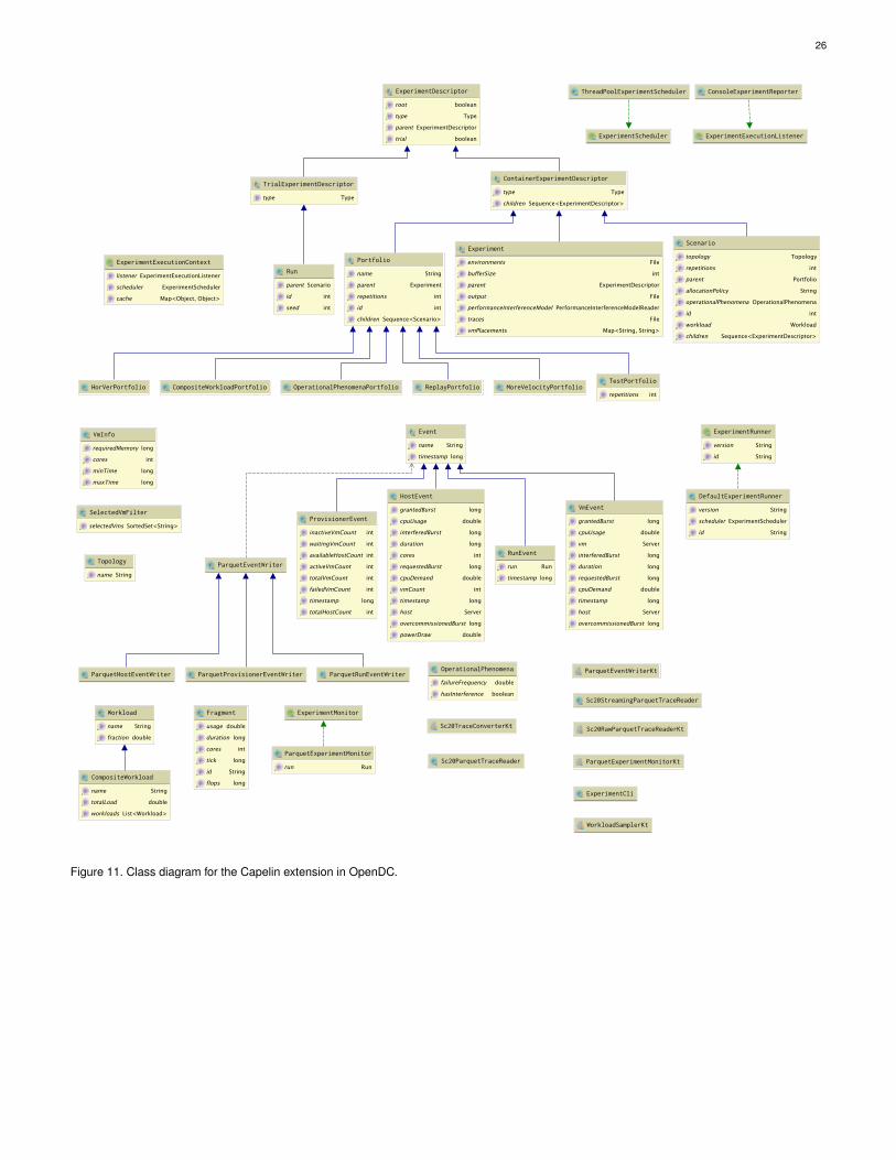
26

ExperimentCli

WorkloadSamplerKt

intrepetitions

TestPortfolio

Sc20ParquetTraceReader

Typetype

TrialExperimentDescriptor

Stringname

longtimestamp

Event

longgrantedBurst

doublecpuUsage

longinterferedBurst

longduration

intcores

longrequestedBurst

doublecpuDemand

intvmCount

longtimestamp

Serverhost

longovercommissionedBurst

doublepowerDraw

HostEvent

SortedSet<String>selectedVms

SelectedVmFilter

Scenarioparent

intid

intseed

Run

Typetype

Sequence<ExperimentDescriptor>children

ContainerExperimentDescriptor

longgrantedBurst

doublecpuUsage

Servervm

longinterferedBurst

longduration

longrequestedBurst

doublecpuDemand

longtimestamp

Serverhost

longovercommissionedBurst

VmEvent

Sc20TraceConverterKt

Topologytopology

intrepetitions

Portfolioparent

StringallocationPolicy

OperationalPhenomenaoperationalPhenomena

intid

Workloadworkload

Sequence<ExperimentDescriptor>children

Scenario

MoreVelocityPortfolioCompositeWorkloadPortfolio

Stringversion

Stringid

ExperimentRunner

ConsoleExperimentReporter

ReplayPortfolio

Sc20StreamingParquetTraceReader

Fileenvironments

intbufferSize

ExperimentDescriptorparent

Fileoutput

PerformanceInterferenceModelReaderperformanceInterferenceModel

Filetraces

Map<String, String>vmPlacements

Experiment

longrequiredMemory

intcores

longminTime

longmaxTime

VmInfo

Sc20RawParquetTraceReaderKt

OperationalPhenomenaPortfolio

Stringname

Experimentparent

intrepetitions

intid

Sequence<Scenario>children

Portfolio

Runrun

longtimestamp

RunEvent

HorVerPortfolio

booleanroot

Typetype

ExperimentDescriptorparent

booleantrial

ExperimentDescriptor

intinactiveVmCount

intwaitingVmCount

intavailableHostCount

intactiveVmCount

inttotalVmCount

intfailedVmCount

longtimestamp

inttotalHostCount

ProvisionerEvent

doubleusage

longduration

intcores

longtick

Stringid

longflops

Fragment

Stringname

doublefraction

Workload

doublefailureFrequency

booleanhasInterference

OperationalPhenomena

ParquetEventWriter

ExperimentScheduler

ParquetRunEventWriter

ExperimentExecutionListener

ThreadPoolExperimentScheduler

Stringname

doubletotalLoad

List<Workload>workloads

CompositeWorkload

ParquetExperimentMonitorKt

Stringname

Topology

ParquetEventWriterKt

ExperimentMonitor

Runrun

ParquetExperimentMonitor

ParquetProvisionerEventWriter

ExperimentExecutionListenerlistener

ExperimentSchedulerscheduler

Map<Object, Object>cache

ExperimentExecutionContext

Stringversion

ExperimentSchedulerscheduler

Stringid

DefaultExperimentRunner

ParquetHostEventWriter

Figure 11. Class diagram for the Capelin extension in OpenDC.

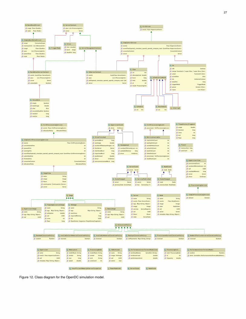
27

ServerState

Nodenode

NodeStatepreviousState

StateChanged

Serverserver

ServerStatepreviousState

StateChanged

Stringname

Flow<ServerEvent>events

Map<String, Object>tags

Imageimage

ServiceRegistryservices

UUIDuid

Flavorflavor

ServerStatestate

Server

StringmodelName

Stringvendor

longsize

doublespeed

MemoryUnit

NodeState

longgrantedBurst

doublecpuUsage

intnumberOfDeployedImages

ServerhostServer

longinterferedBurst

longrequestedBurst

doublecpuDemand

VirtDriverdriver

longovercommissionedBurst

SliceFinished

Serverserver

ServerEvent

VirtDriverdriver

HypervisorEvent

Stringname

Flow<HypervisorEvent>events

UUIDuid

Map<String, Object>metadata

Hypervisor

longmemorySize

intcpuCount

Flavor

Nodenode

NodeEvent

Stringname

Flow<NodeEvent>events

Imageimage

NodeStatestate

UUIDuid

Serverserver

Map<String, Object>metadata

Node

ProcessingNodenode

intid

doublefrequency

ProcessingUnit

Stringname

Map<String, Object>tags

UUIDuid

HypervisorImage

Serverserver

ServiceKey<?>key

ServicePublished

StringmodelName

Stringvendor

Stringarch

intcoreCount

ProcessingNode

intnumberOfActiveServers

longavailableMemory

VirtDriverdriver

VmsUpdated

Vmvm

Schedule

Randomrandom

SortedSet<PerformanceInterferenceModelItem>items

PerformanceInterferenceModel

List<ProcessingUnit>cpus

Serverserver

ServerContext

Stringname

VmImageimage

UUIDuid

Userowner

VmWorkload

Vmvm

doubleallocatedLimit

longburst

doublelimit

intid

ProcessingUnitmodel

VCpu

EventFlow<ServerEvent>events

List<ProcessingUnit>cpus

Jobjob$opendc_simulator_opendc_opendc_compute_main

Serverserver

VmServerContext

SchedulerCommand

booleanidle

Function2<? super Slice, ? super Slice, Slice>merge

Function0<Unit>select

SliceactiveSlice

VmServerContextctx

longdeadline

TriggerModetriggerMode

Iterator<Slice>queue

List<VCpu>vcpus

Vm

Vmvm

Deschedule

ProvisioningService

Flow<HypervisorEvent>events

EventFlow<HypervisorEvent>eventFlow$opendc_simulator_opendc_opendc_compute_main

CoroutineContextcoroutineContext

Serverserver

SimpleVirtDriver

Stringname

Map<String, Object>tags

UUIDuid

EmptyImageStringname

Map<String, Object>tags

doubleutilization

UUIDuid

intcores

longflops

FlopsApplicationImage

Flow<VirtProvisioningEvent>events

intunscheduledVms

intqueuedVms

intrunningVms

EventFlow<VirtProvisioningEvent>eventFlow$opendc_simulator_opendc_opendc_compute_main

intsubmittedVms

intfinishedVms

CoroutineContextcoroutineContext

AllocationPolicyallocationPolicy

SimpleVirtProvisioningService

Stringname

Imageimage

Flavorflavor

Continuation<Server>continuation

Serverserver

ImageView

intprovisionedCores

intnumberOfActiveServers

UUIDuid

longavailableMemory

Serverserver

VirtDriverdriver

HypervisorView

Flow<VirtProvisioningEvent>events

AllocationPolicyallocationPolicy

VirtProvisioningServicedoubleusage

longduration

intcores

longtick

longflops

FlopsHistoryFragment

VirtProvisioningServiceprovisioner

VirtProvisioningEvent

Flow<HypervisorEvent>events

VirtDriverFlow<Double>usage

Flow<Node>node

BareMetalDriver

CoroutineScopescope

List<MemoryUnit>memoryUnits

Flow<Double>usage

List<ProcessingUnit>cpus

Flow<Double>powerDraw

Flow<Node>node

SimpleBareMetalDriver

Stringname

Map<String, Object>tags

intmaxCores

longrequiredMemory

UUIDuid

Sequence<FlopsHistoryFragment>flopsHistory

VmImage

SortedSet<String>workloadNames

doubleminServerLoad

doubleperformanceScore

PerformanceInterferenceModelItem

Image

EventFlow<ServerEvent>events

List<ProcessingUnit>cpus

Serverserver

booleanunavailable

BareMetalServerContext

booleanempty

doubletotalUsage

Sliceslice

booleanexceedsDeadline

longmaxExit

longminExit

SliceWork

InsufficientMemoryOnServerException PowerModelsKt

Interrupt

TriggerMode ServerManagementContext

Domaindomain

SimpleProvisioningService

double[]limit

long[]burst

longdeadline

Slice

AllocationPolicy

booleanreversed

AvailableCoreMemoryAllocationPolicy

booleanreversed

NumberOfActiveServersAllocationPolicy

booleanreversed

ProvisionedCoresAllocationPolicy

Map<String, String>vmPlacements

ReplayAllocationPolicy

booleanreversed

AvailableMemoryAllocationPolicy

Randomrandom

RandomAllocationPolicy

intinactiveVmCount

intwaitingVmCount

intavailableHostCount

intactiveVmCount

inttotalVmCount

intfailedVmCount

VirtProvisioningServiceprovisioner

inttotalHostCount

MetricsAvailable

Figure 12. Class diagram for the OpenDC simulation model.

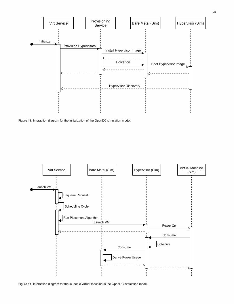
28

Virt Service

InitializeProvision Hypervisors

ProvisioningService

Install Hypervisor Image

Hypervisor (Sim)Bare Metal (Sim)

Boot Hypervisor ImagePower on

Hypervisor Discovery

Figure 13. Interaction diagram for the initialization of the OpenDC simulation model.

Virt Service

Launch VM

Enqueue Request

Scheduling Cycle

Hypervisor (Sim)

Power On

Schedule

Bare Metal (Sim) Virtual Machine(Sim)

Run Placement AlgorithmLaunch VM

Consume

Consume

Derive Power Usage

Figure 14. Interaction diagram for the launch a virtual machine in the OpenDC simulation model.

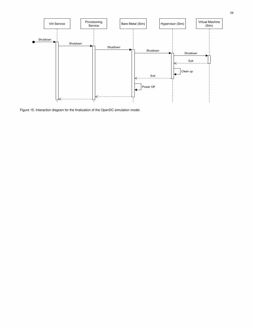
29

Virt Service

ShutdownShutdown

ProvisioningService Hypervisor (Sim)Bare Metal (Sim)

Power Off

Virtual Machine(Sim)

Shutdown

Exit

Exit

ShutdownShutdown

Clean up

Figure 15. Interaction diagram for the finalization of the OpenDC simulation model.

30

APPENDIX DFULL VISUAL RESULTS

In the figures below, we visualize the full set of metrics(§5.1.7) for each experiment. We differentiate between se-lect overviews (depicting only the results of a subset ofworkloads) and summary overviews (aggregating over allworkloads).

31

(a) Requested CPU cycles (b) Granted CPU cycles

(c) Overcommitted CPU cycles (d) Interfered CPU cycles

(e) Total power consumption (f) Total number of time slices in which a VM is failed, aggregated acrossVMs

Figure 16. Performance of different horizontally and vertically expanded topologies, compared across workloads. For a legend of topologies, seeTable 2. Continued in Figure 17.

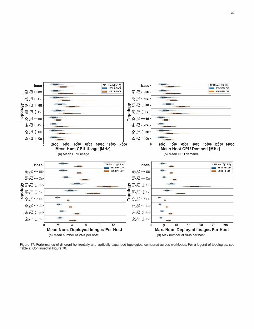
32

(a) Mean CPU usage (b) Mean CPU demand

(c) Mean number of VMs per host (d) Max number of VMs per host

Figure 17. Performance of different horizontally and vertically expanded topologies, compared across workloads. For a legend of topologies, seeTable 2. Continued in Figure 18.

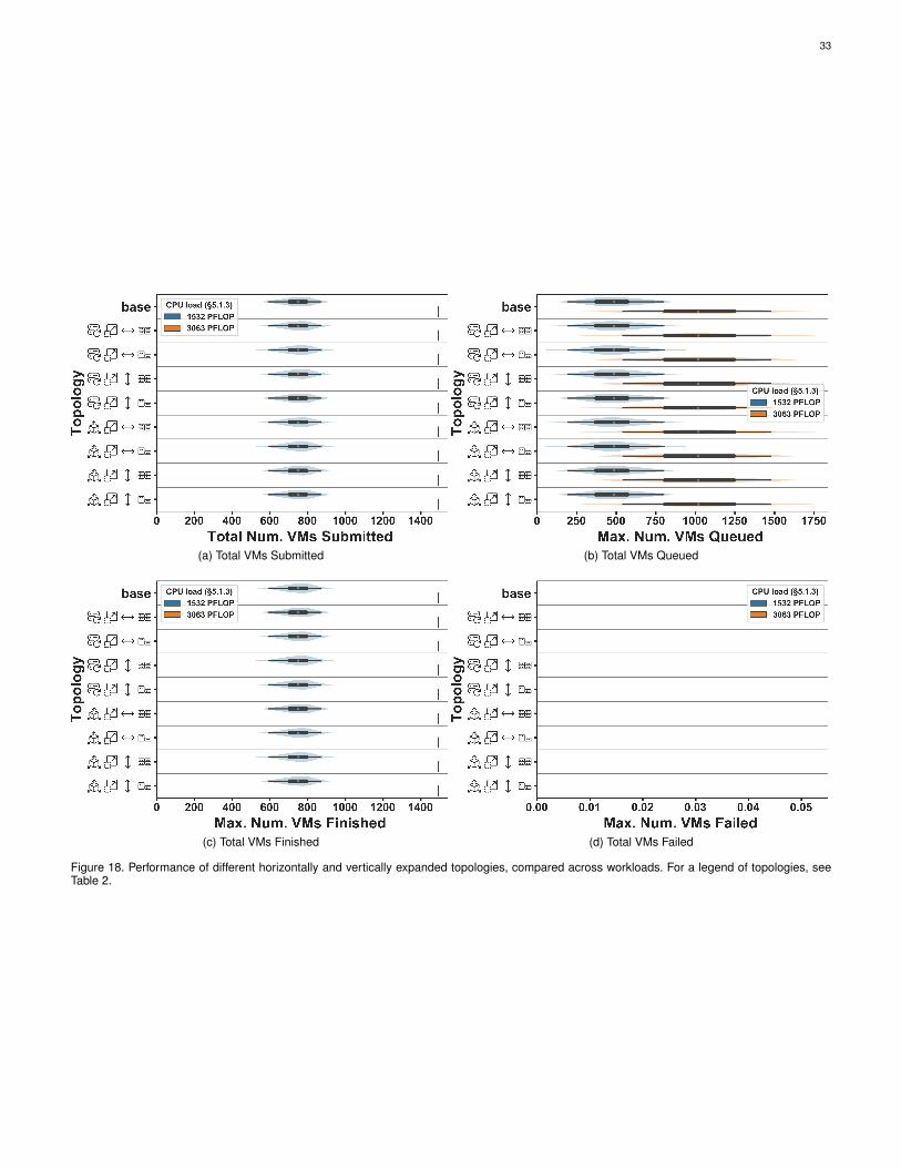
33

(a) Total VMs Submitted (b) Total VMs Queued

(c) Total VMs Finished (d) Total VMs Failed

Figure 18. Performance of different horizontally and vertically expanded topologies, compared across workloads. For a legend of topologies, seeTable 2.

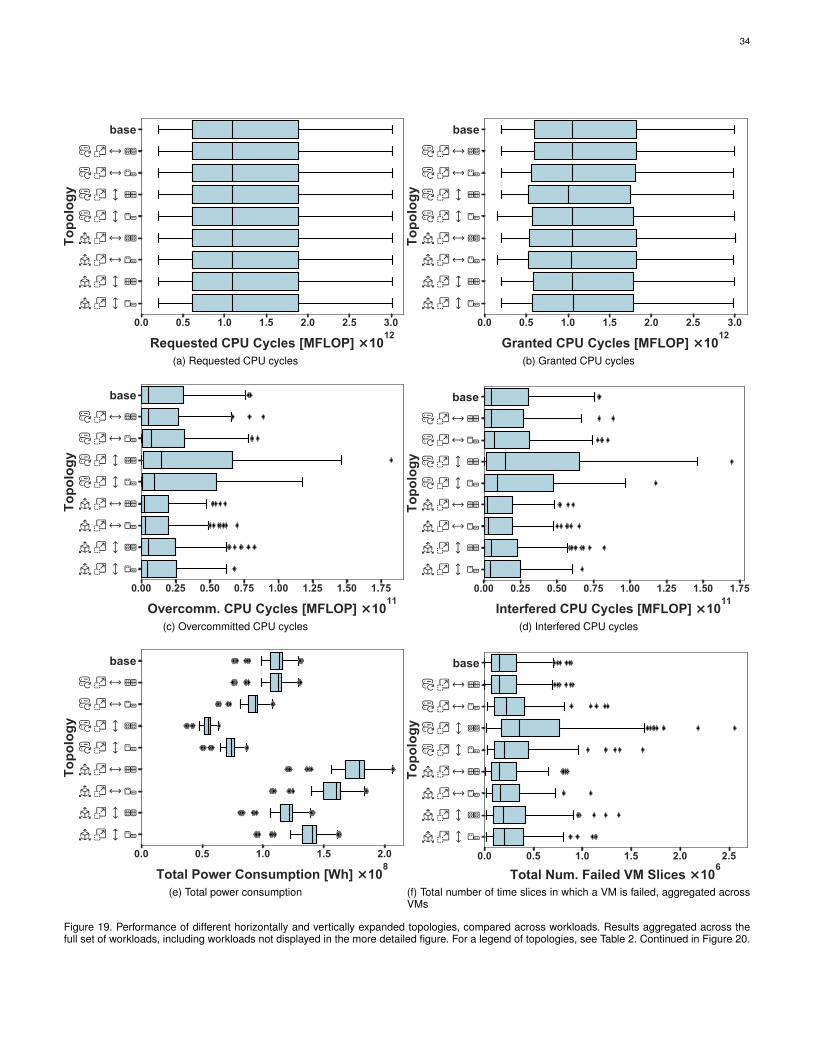
34

0.0 0.5 1.0 1.5 2.0 2.5 3.0

Requested CPU Cycles [MFLOP] ×1012

base

E H D C

E H D B

E H G C

E H G B

A H D C

A H D B

A H G C

A H G B

To

po

log

y

(a) Requested CPU cycles

0.0 0.5 1.0 1.5 2.0 2.5 3.0

Granted CPU Cycles [MFLOP] ×1012

base

E H D C

E H D B

E H G C

E H G B

A H D C

A H D B

A H G C

A H G B

To

po

log

y

(b) Granted CPU cycles

0.00 0.25 0.50 0.75 1.00 1.25 1.50 1.75

Overcomm. CPU Cycles [MFLOP] ×1011

base

E H D C

E H D B

E H G C

E H G B

A H D C

A H D B

A H G C

A H G B

To

po

log

y

(c) Overcommitted CPU cycles

0.00 0.25 0.50 0.75 1.00 1.25 1.50 1.75

Interfered CPU Cycles [MFLOP] ×1011

base

E H D C

E H D B

E H G C

E H G B

A H D C

A H D B

A H G C

A H G B

To

po

log

y

(d) Interfered CPU cycles

0.0 0.5 1.0 1.5 2.0

Total Power Consumption [Wh] ×108

base

E H D C

E H D B

E H G C

E H G B

A H D C

A H D B

A H G C

A H G B

To

po

log

y

(e) Total power consumption

0.0 0.5 1.0 1.5 2.0 2.5

Total Num. Failed VM Slices ×106

base

E H D C

E H D B

E H G C

E H G B

A H D C

A H D B

A H G C

A H G B

To

po

log

y

(f) Total number of time slices in which a VM is failed, aggregated acrossVMs

Figure 19. Performance of different horizontally and vertically expanded topologies, compared across workloads. Results aggregated across thefull set of workloads, including workloads not displayed in the more detailed figure. For a legend of topologies, see Table 2. Continued in Figure 20.

35

0 2000 4000 6000 8000 10000 12000

Mean Host CPU Usage [MHz]

base

E H D C

E H D B

E H G C

E H G B

A H D C

A H D B

A H G C

A H G B

To

po

log

y

(a) Mean CPU usage

0 2000 4000 6000 8000 10000 12000

Mean Host CPU Demand [MHz]

base

E H D C

E H D B

E H G C

E H G B

A H D C

A H D B

A H G C

A H G B

To

po

log

y

(b) Mean CPU demand

0 2 4 6 8 10

Mean Num. Deployed Images Per Host

base

E H D C

E H D B

E H G C

E H G B

A H D C

A H D B

A H G C

A H G B

To

po

log

y

(c) Mean number of VMs per host

0 5 10 15 20 25

Max. Num. Deployed Images Per Host

base

E H D C

E H D B

E H G C

E H G B

A H D C

A H D B

A H G C

A H G B

To

po

log

y

(d) Max number of VMs per host

Figure 20. Performance of different horizontally and vertically expanded topologies, compared across workloads. Results aggregated across thefull set of workloads, including workloads not displayed in the more detailed figure. For a legend of topologies, see Table 2. Continued in Figure 21.

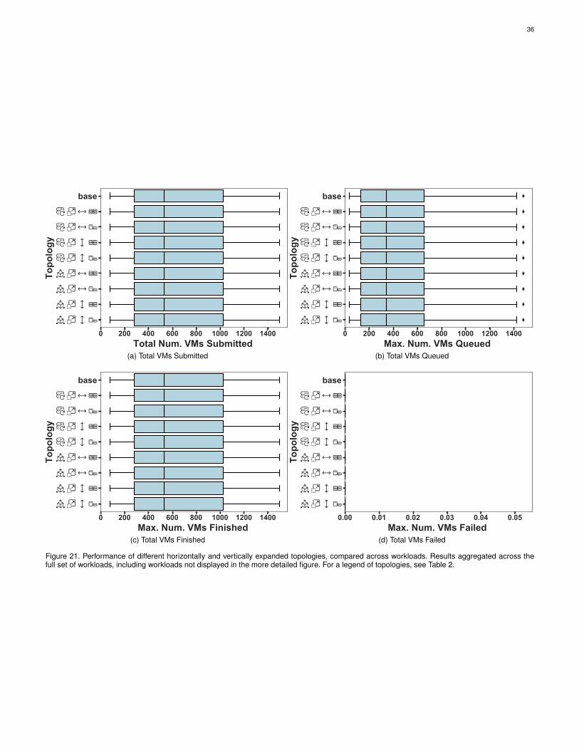
36

0 200 400 600 800 1000 1200 1400

Total Num. VMs Submitted

base

E H D C

E H D B

E H G C

E H G B

A H D C

A H D B

A H G C

A H G B

To

po

log

y

(a) Total VMs Submitted

0 200 400 600 800 1000 1200 1400

Max. Num. VMs Queued

base

E H D C

E H D B

E H G C

E H G B

A H D C

A H D B

A H G C

A H G B

To

po

log

y

(b) Total VMs Queued

0 200 400 600 800 1000 1200 1400

Max. Num. VMs Finished

base

E H D C

E H D B

E H G C

E H G B

A H D C

A H D B

A H G C

A H G B

To

po

log

y

(c) Total VMs Finished

0.00 0.01 0.02 0.03 0.04 0.05

Max. Num. VMs Failed

base

E H D C

E H D B

E H G C

E H G B

A H D C

A H D B

A H G C

A H G B

To

po

log

y

(d) Total VMs Failed

Figure 21. Performance of different horizontally and vertically expanded topologies, compared across workloads. Results aggregated across thefull set of workloads, including workloads not displayed in the more detailed figure. For a legend of topologies, see Table 2.

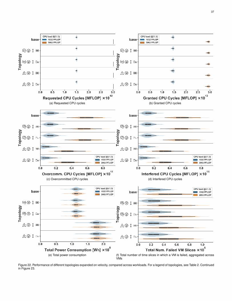
37

(a) Requested CPU cycles (b) Granted CPU cycles

(c) Overcommitted CPU cycles (d) Interfered CPU cycles

(e) Total power consumption (f) Total number of time slices in which a VM is failed, aggregated acrossVMs

Figure 22. Performance of different topologies expanded on velocity, compared across workloads. For a legend of topologies, see Table 2. Continuedin Figure 23.

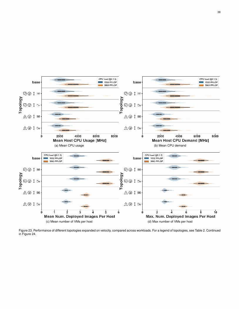
38

(a) Mean CPU usage (b) Mean CPU demand

(c) Mean number of VMs per host (d) Max number of VMs per host

Figure 23. Performance of different topologies expanded on velocity, compared across workloads. For a legend of topologies, see Table 2. Continuedin Figure 24.

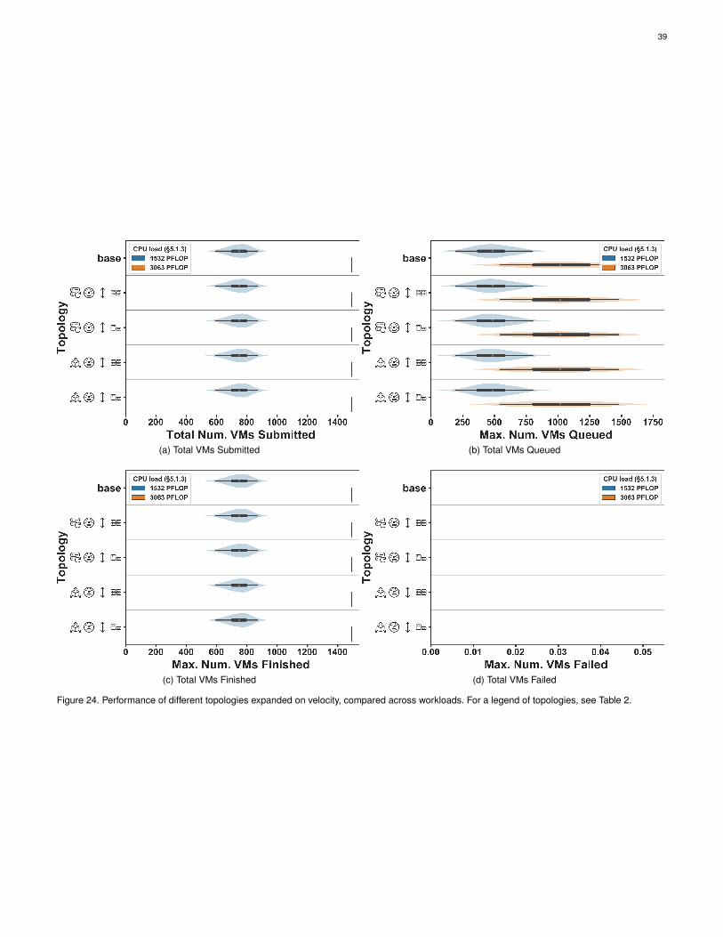
39

(a) Total VMs Submitted (b) Total VMs Queued

(c) Total VMs Finished (d) Total VMs Failed

Figure 24. Performance of different topologies expanded on velocity, compared across workloads. For a legend of topologies, see Table 2.

40

0.0 0.5 1.0 1.5 2.0 2.5 3.0

Requested CPU Cycles [MFLOP] ×1012

base

E F G C

E F G B

A F G C

A F G B

To

po

log

y

(a) Requested CPU cycles

0.0 0.5 1.0 1.5 2.0 2.5 3.0

Granted CPU Cycles [MFLOP] ×1012

base

E F G C

E F G B

A F G C

A F G B

To

po

log

y

(b) Granted CPU cycles

0.0 0.2 0.4 0.6 0.8

Overcomm. CPU Cycles [MFLOP] ×1011

base

E F G C

E F G B

A F G C

A F G B

To

po

log

y

(c) Overcommitted CPU cycles

0.0 0.2 0.4 0.6 0.8

Interfered CPU Cycles [MFLOP] ×1011

base

E F G C

E F G B

A F G C

A F G B

To

po

log

y

(d) Interfered CPU cycles

0.0 0.5 1.0 1.5 2.0

Total Power Consumption [Wh] ×108

base

E F G C

E F G B

A F G C

A F G B

To

po

log

y

(e) Total power consumption

0.0 0.2 0.4 0.6 0.8

Total Num. Failed VM Slices ×106

base

E F G C

E F G B

A F G C

A F G B

To

po

log

y

(f) Total number of time slices in which a VM is failed, aggregated acrossVMs

Figure 25. Performance of different topologies expanded on velocity, compared across workloads. Results aggregated across the full set ofworkloads, including workloads not displayed in the more detailed figure. For a legend of topologies, see Table 2. Continued in Figure 26.

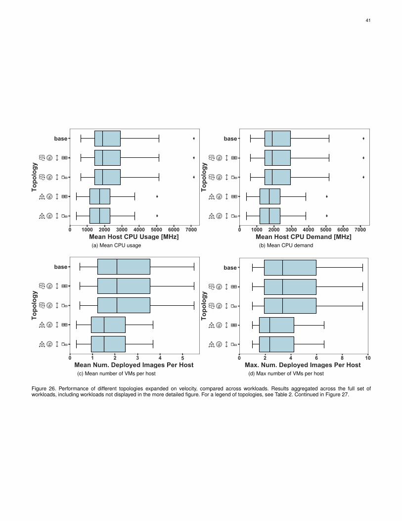
41

0 1000 2000 3000 4000 5000 6000 7000

Mean Host CPU Usage [MHz]

base

E F G C

E F G B

A F G C

A F G B

To

po

log

y

(a) Mean CPU usage

0 1000 2000 3000 4000 5000 6000 7000

Mean Host CPU Demand [MHz]

base

E F G C

E F G B

A F G C

A F G B

To

po

log

y

(b) Mean CPU demand

0 1 2 3 4 5

Mean Num. Deployed Images Per Host

base

E F G C

E F G B

A F G C

A F G B

To

po

log

y

(c) Mean number of VMs per host

0 2 4 6 8 10

Max. Num. Deployed Images Per Host

base

E F G C

E F G B

A F G C

A F G B

To

po

log

y

(d) Max number of VMs per host

Figure 26. Performance of different topologies expanded on velocity, compared across workloads. Results aggregated across the full set ofworkloads, including workloads not displayed in the more detailed figure. For a legend of topologies, see Table 2. Continued in Figure 27.

42

0 200 400 600 800 1000 1200 1400

Total Num. VMs Submitted

base

E F G C

E F G B

A F G C

A F G B

To

po

log

y

(a) Total VMs Submitted

0 200 400 600 800 1000 1200 1400

Max. Num. VMs Queued

base

E F G C

E F G B

A F G C

A F G B

To

po

log

y

(b) Total VMs Queued

0 200 400 600 800 1000 1200 1400

Max. Num. VMs Finished

base

E F G C

E F G B

A F G C

A F G B

To

po

log

y

(c) Total VMs Finished

0.00 0.01 0.02 0.03 0.04 0.05

Max. Num. VMs Failed

base

E F G C

E F G B

A F G C

A F G B

To

po

log

y

(d) Total VMs Failed

Figure 27. Performance of different topologies expanded on velocity, compared across workloads. Results aggregated across the full set ofworkloads, including workloads not displayed in the more detailed figure. For a legend of topologies, see Table 2.

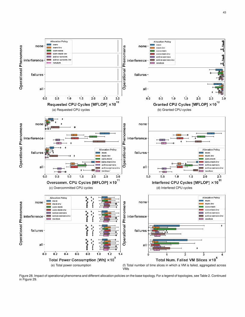
43

(a) Requested CPU cycles (b) Granted CPU cycles

(c) Overcommitted CPU cycles (d) Interfered CPU cycles

(e) Total power consumption (f) Total number of time slices in which a VM is failed, aggregated acrossVMs

Figure 28. Impact of operational phenomena and different allocation policies on the base topology. For a legend of topologies, see Table 2. Continuedin Figure 29.

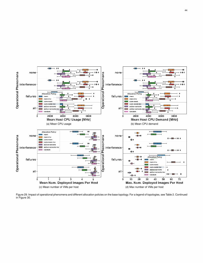
44

(a) Mean CPU usage (b) Mean CPU demand

(c) Mean number of VMs per host (d) Max number of VMs per host

Figure 29. Impact of operational phenomena and different allocation policies on the base topology. For a legend of topologies, see Table 2. Continuedin Figure 30.

45

(a) Total VMs Submitted (b) Total VMs Queued

(c) Total VMs Finished (d) Total VMs Failed

Figure 30. Impact of operational phenomena and different allocation policies on the base topology. For a legend of topologies, see Table 2.

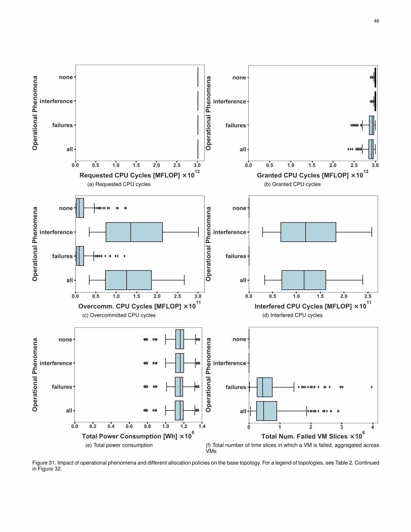
46

0.0 0.5 1.0 1.5 2.0 2.5 3.0

Requested CPU Cycles [MFLOP] ×1012

none

interference

failures

allOp

era

tio

na

l P

he

no

me

na

(a) Requested CPU cycles

0.0 0.5 1.0 1.5 2.0 2.5 3.0

Granted CPU Cycles [MFLOP] ×1012

none

interference

failures

allOp

era

tio

na

l P

he

no

me

na

(b) Granted CPU cycles

0.0 0.5 1.0 1.5 2.0 2.5 3.0

Overcomm. CPU Cycles [MFLOP] ×1011

none

interference

failures

allOp

era

tio

na

l P

he

no

me

na

(c) Overcommitted CPU cycles

0.0 0.5 1.0 1.5 2.0 2.5

Interfered CPU Cycles [MFLOP] ×1011

none

interference

failures

allOp

era

tio

na

l P

he

no

me

na

(d) Interfered CPU cycles

0.0 0.2 0.4 0.6 0.8 1.0 1.2 1.4

Total Power Consumption [Wh] ×108

none

interference

failures

allOp

era

tio

na

l P

he

no

me

na

(e) Total power consumption

0 1 2 3 4

Total Num. Failed VM Slices ×106

none

interference

failures

allOp

era

tio

na

l P

he

no

me

na

(f) Total number of time slices in which a VM is failed, aggregated acrossVMs

Figure 31. Impact of operational phenomena and different allocation policies on the base topology. For a legend of topologies, see Table 2. Continuedin Figure 32.

47

0 2000 4000 6000 8000

Mean Host CPU Usage [MHz]

none

interference

failures

allOp

era

tio

na

l P

he

no

me

na

(a) Mean CPU usage

0 2000 4000 6000 8000

Mean Host CPU Demand [MHz]

none

interference

failures

allOp

era

tio

na

l P

he

no

me

na

(b) Mean CPU demand

0 1 2 3 4 5

Mean Num. Deployed Images Per Host

none

interference

failures

allOp

era

tio

na

l P

he

no

me

na

(c) Mean number of VMs per host

0 10 20 30 40 50 60 70

Max. Num. Deployed Images Per Host

none

interference

failures

allOp

era

tio

na

l P

he

no

me

na

(d) Max number of VMs per host

Figure 32. Impact of operational phenomena and different allocation policies on the base topology. For a legend of topologies, see Table 2. Continuedin Figure 33.

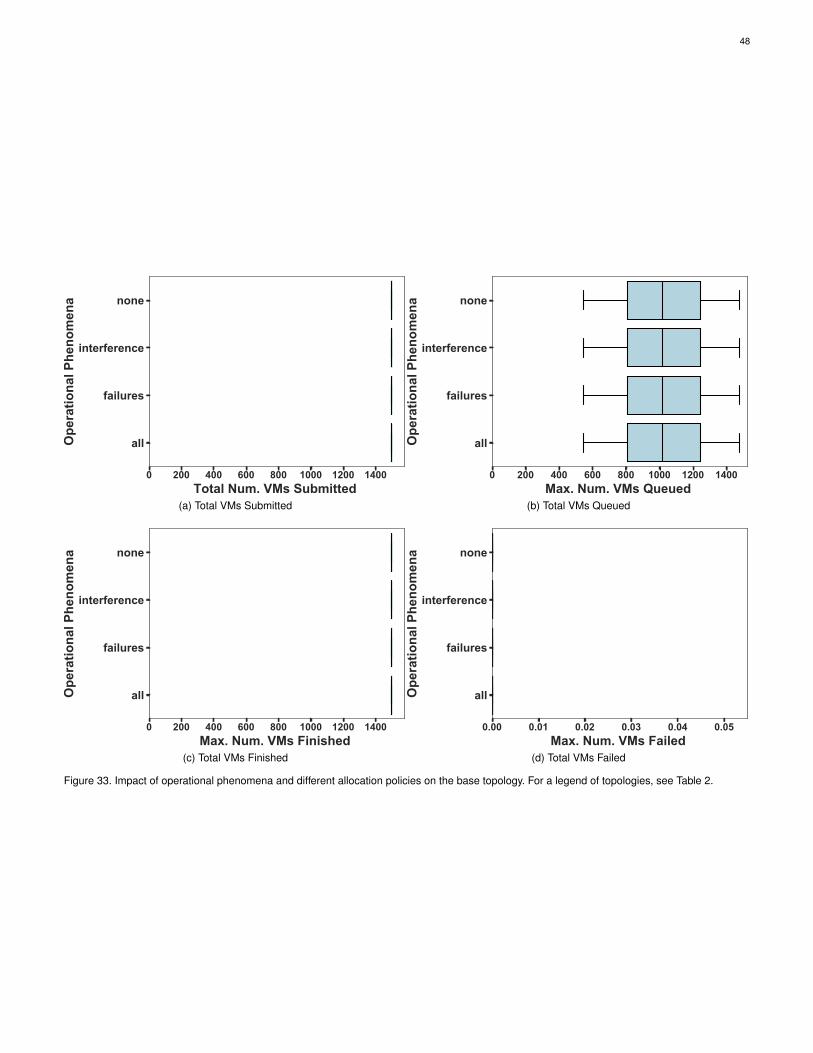
48

0 200 400 600 800 1000 1200 1400

Total Num. VMs Submitted

none

interference

failures

allOp

era

tio

na

l P

he

no

me

na

(a) Total VMs Submitted

0 200 400 600 800 1000 1200 1400

Max. Num. VMs Queued

none

interference

failures

allOp

era

tio

na

l P

he

no

me

na

(b) Total VMs Queued

0 200 400 600 800 1000 1200 1400

Max. Num. VMs Finished

none

interference

failures

allOp

era

tio

na

l P

he

no

me

na

(c) Total VMs Finished

0.00 0.01 0.02 0.03 0.04 0.05

Max. Num. VMs Failed

none

interference

failures

allOp

era

tio

na

l P

he

no

me

na

(d) Total VMs Failed

Figure 33. Impact of operational phenomena and different allocation policies on the base topology. For a legend of topologies, see Table 2.

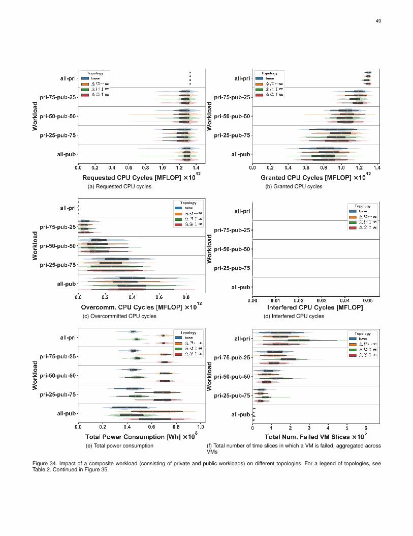
49

(a) Requested CPU cycles (b) Granted CPU cycles

(c) Overcommitted CPU cycles (d) Interfered CPU cycles

(e) Total power consumption (f) Total number of time slices in which a VM is failed, aggregated acrossVMs

Figure 34. Impact of a composite workload (consisting of private and public workloads) on different topologies. For a legend of topologies, seeTable 2. Continued in Figure 35.

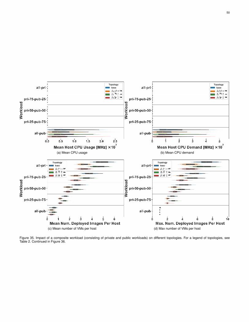
50

(a) Mean CPU usage (b) Mean CPU demand

(c) Mean number of VMs per host (d) Max number of VMs per host

Figure 35. Impact of a composite workload (consisting of private and public workloads) on different topologies. For a legend of topologies, seeTable 2. Continued in Figure 36.

51

(a) Total VMs Submitted (b) Total VMs Queued

(c) Total VMs Finished (d) Total VMs Failed

Figure 36. Impact of a composite workload (consisting of private and public workloads) on different topologies. For a legend of topologies, seeTable 2.

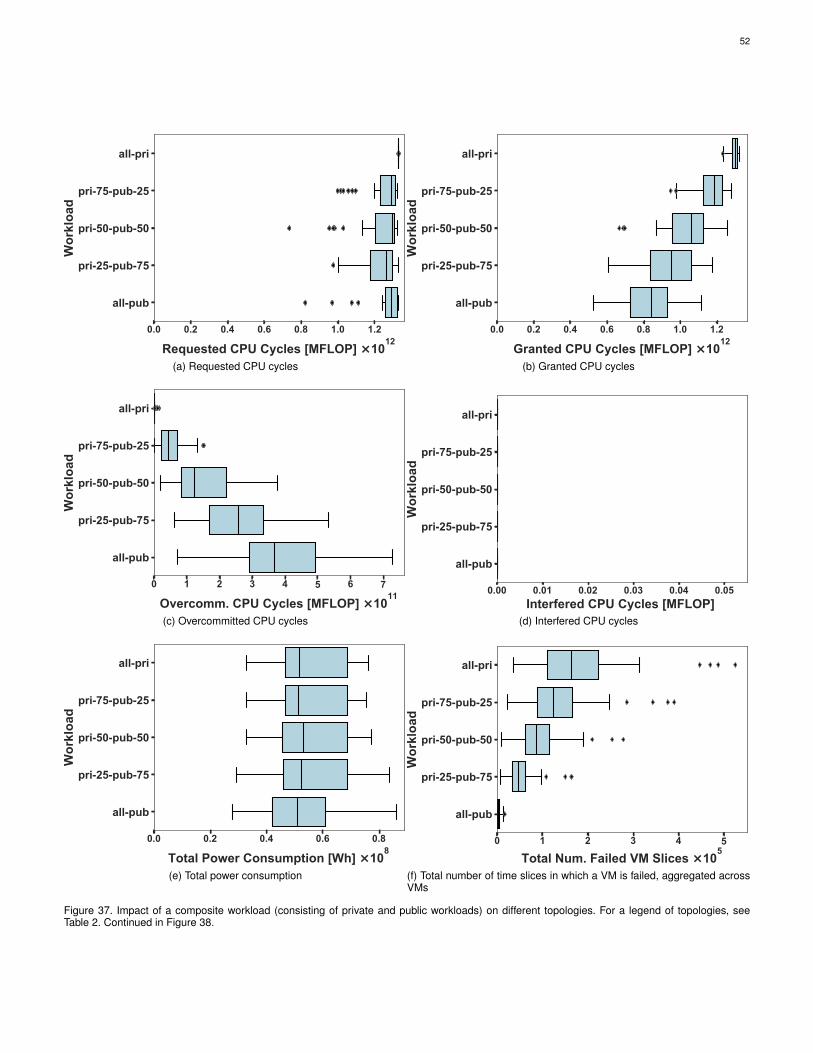
52

0.0 0.2 0.4 0.6 0.8 1.0 1.2

Requested CPU Cycles [MFLOP] ×1012

all-pri

pri-75-pub-25

pri-50-pub-50

pri-25-pub-75

all-pub

Wo

rklo

ad

(a) Requested CPU cycles

0.0 0.2 0.4 0.6 0.8 1.0 1.2

Granted CPU Cycles [MFLOP] ×1012

all-pri

pri-75-pub-25

pri-50-pub-50

pri-25-pub-75

all-pub

Wo

rklo

ad

(b) Granted CPU cycles

0 1 2 3 4 5 6 7

Overcomm. CPU Cycles [MFLOP] ×1011

all-pri

pri-75-pub-25

pri-50-pub-50

pri-25-pub-75

all-pub

Wo

rklo

ad

(c) Overcommitted CPU cycles

0.00 0.01 0.02 0.03 0.04 0.05

Interfered CPU Cycles [MFLOP]

all-pri

pri-75-pub-25

pri-50-pub-50

pri-25-pub-75

all-pub

Wo

rklo

ad

(d) Interfered CPU cycles

0.0 0.2 0.4 0.6 0.8

Total Power Consumption [Wh] ×108

all-pri

pri-75-pub-25

pri-50-pub-50

pri-25-pub-75

all-pub

Wo

rklo

ad

(e) Total power consumption

0 1 2 3 4 5

Total Num. Failed VM Slices ×105

all-pri

pri-75-pub-25

pri-50-pub-50

pri-25-pub-75

all-pub

Wo

rklo

ad

(f) Total number of time slices in which a VM is failed, aggregated acrossVMs

Figure 37. Impact of a composite workload (consisting of private and public workloads) on different topologies. For a legend of topologies, seeTable 2. Continued in Figure 38.

53

0.0 0.5 1.0 1.5 2.0

Mean Host CPU Usage [MHz] ×107

all-pri

pri-75-pub-25

pri-50-pub-50

pri-25-pub-75

all-pub

Wo

rklo

ad

(a) Mean CPU usage

0 1 2 3 4

Mean Host CPU Demand [MHz] ×107

all-pri

pri-75-pub-25

pri-50-pub-50

pri-25-pub-75

all-pub

Wo

rklo

ad

(b) Mean CPU demand

0 1 2 3 4 5 6

Mean Num. Deployed Images Per Host

all-pri

pri-75-pub-25

pri-50-pub-50

pri-25-pub-75

all-pub

Wo

rklo

ad

(c) Mean number of VMs per host

0 2 4 6 8

Max. Num. Deployed Images Per Host

all-pri

pri-75-pub-25

pri-50-pub-50

pri-25-pub-75

all-pub

Wo

rklo

ad

(d) Max number of VMs per host

Figure 38. Impact of a composite workload (consisting of private and public workloads) on different topologies. For a legend of topologies, seeTable 2. Continued in Figure 39.

54

0 200 400 600 800 1000 1200 1400

Total Num. VMs Submitted

all-pri

pri-75-pub-25

pri-50-pub-50

pri-25-pub-75

all-pub

Wo

rklo

ad

(a) Total VMs Submitted

0 200 400 600 800 1000 1200 1400

Max. Num. VMs Queued

all-pri

pri-75-pub-25

pri-50-pub-50

pri-25-pub-75

all-pub

Wo

rklo

ad

(b) Total VMs Queued

0 200 400 600 800 1000 1200 1400

Max. Num. VMs Finished

all-pri

pri-75-pub-25

pri-50-pub-50

pri-25-pub-75

all-pub

Wo

rklo

ad

(c) Total VMs Finished

0.00 0.01 0.02 0.03 0.04 0.05

Max. Num. VMs Failed

all-pri

pri-75-pub-25

pri-50-pub-50

pri-25-pub-75

all-pub

Wo

rklo

ad

(d) Total VMs Failed

Figure 39. Impact of a composite workload (consisting of private and public workloads) on different topologies. For a legend of topologies, seeTable 2.

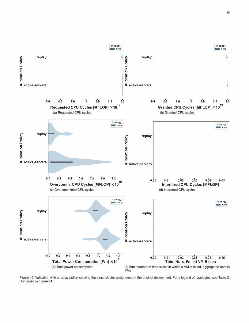
55

(a) Requested CPU cycles (b) Granted CPU cycles

(c) Overcommitted CPU cycles (d) Interfered CPU cycles

(e) Total power consumption (f) Total number of time slices in which a VM is failed, aggregated acrossVMs

Figure 40. Validation with a replay policy, copying the exact cluster assignment of the original deployment. For a legend of topologies, see Table 2.Continued in Figure 41.

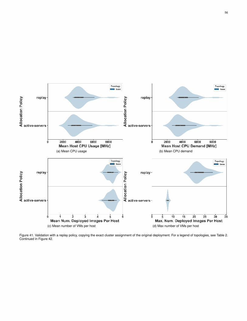
56

(a) Mean CPU usage (b) Mean CPU demand

(c) Mean number of VMs per host (d) Max number of VMs per host

Figure 41. Validation with a replay policy, copying the exact cluster assignment of the original deployment. For a legend of topologies, see Table 2.Continued in Figure 42.

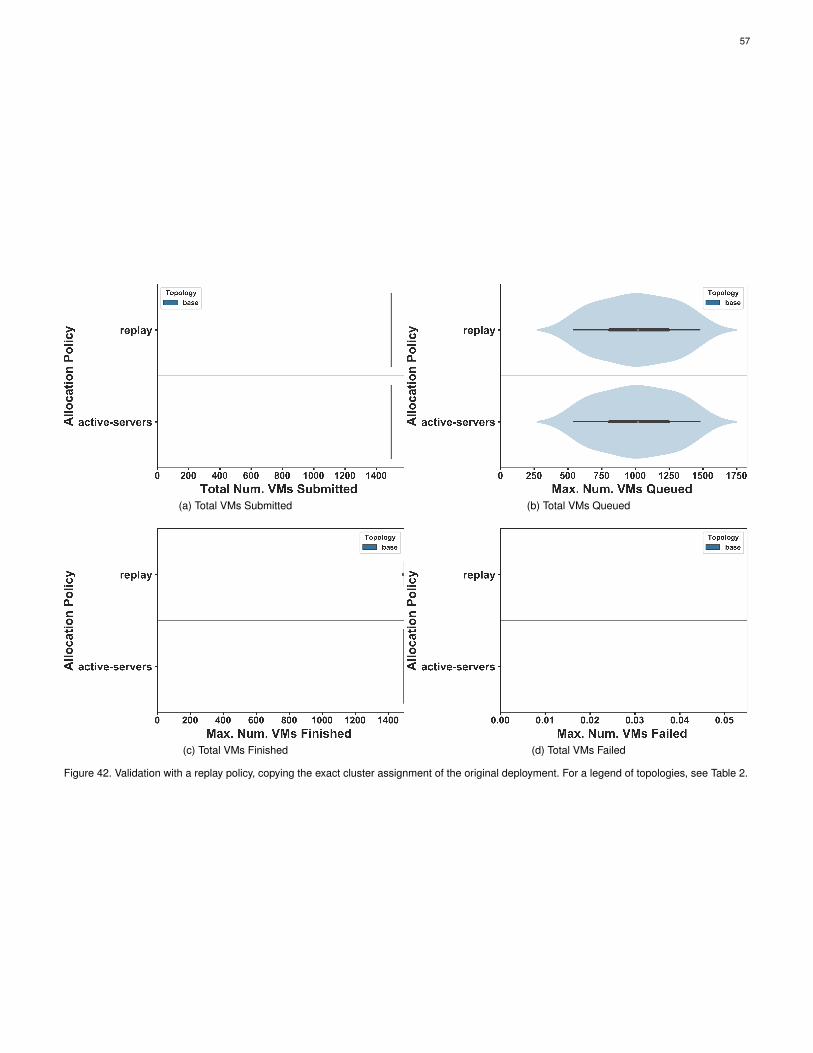
57

(a) Total VMs Submitted (b) Total VMs Queued

(c) Total VMs Finished (d) Total VMs Failed

Figure 42. Validation with a replay policy, copying the exact cluster assignment of the original deployment. For a legend of topologies, see Table 2.

58

APPENDIX EFULL TABULAR RESULTS

In the tables below, we list the full results of two of the mostimportant metrics (§5.1.7) for each experiment: overcommis-sion and power consumption.

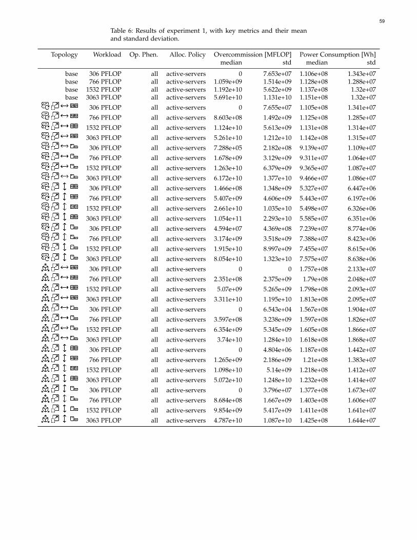
59

Table 6: Results of experiment 1, with key metrics and their meanand standard deviation.

Topology Workload Op. Phen. Alloc. Policy Overcommission [MFLOP] Power Consumption [Wh]median std median std

base 306 PFLOP all active-servers 0 7.653e+07 1.106e+08 1.343e+07base 766 PFLOP all active-servers 1.059e+09 1.514e+09 1.128e+08 1.288e+07base 1532 PFLOP all active-servers 1.192e+10 5.622e+09 1.137e+08 1.32e+07base 3063 PFLOP all active-servers 5.691e+10 1.131e+10 1.151e+08 1.32e+07

306 PFLOP all active-servers 0 7.655e+07 1.105e+08 1.341e+07

766 PFLOP all active-servers 8.603e+08 1.492e+09 1.125e+08 1.285e+07

1532 PFLOP all active-servers 1.124e+10 5.613e+09 1.131e+08 1.314e+07

3063 PFLOP all active-servers 5.261e+10 1.212e+10 1.142e+08 1.315e+07

306 PFLOP all active-servers 7.288e+05 2.182e+08 9.139e+07 1.109e+07

766 PFLOP all active-servers 1.678e+09 3.129e+09 9.311e+07 1.064e+07

1532 PFLOP all active-servers 1.263e+10 6.379e+09 9.365e+07 1.087e+07

3063 PFLOP all active-servers 6.172e+10 1.377e+10 9.466e+07 1.086e+07

306 PFLOP all active-servers 1.466e+08 1.348e+09 5.327e+07 6.447e+06

766 PFLOP all active-servers 5.407e+09 4.606e+09 5.443e+07 6.197e+06

1532 PFLOP all active-servers 2.661e+10 1.035e+10 5.498e+07 6.326e+06

3063 PFLOP all active-servers 1.054e+11 2.293e+10 5.585e+07 6.351e+06

306 PFLOP all active-servers 4.594e+07 4.369e+08 7.239e+07 8.774e+06

766 PFLOP all active-servers 3.174e+09 3.518e+09 7.388e+07 8.423e+06

1532 PFLOP all active-servers 1.915e+10 8.997e+09 7.455e+07 8.615e+06

3063 PFLOP all active-servers 8.054e+10 1.323e+10 7.575e+07 8.638e+06

306 PFLOP all active-servers 0 0 1.757e+08 2.133e+07

766 PFLOP all active-servers 2.351e+08 2.375e+09 1.79e+08 2.048e+07

1532 PFLOP all active-servers 5.07e+09 5.265e+09 1.798e+08 2.093e+07

3063 PFLOP all active-servers 3.311e+10 1.195e+10 1.813e+08 2.095e+07

306 PFLOP all active-servers 0 6.543e+04 1.567e+08 1.904e+07

766 PFLOP all active-servers 3.597e+08 3.238e+09 1.597e+08 1.826e+07

1532 PFLOP all active-servers 6.354e+09 5.345e+09 1.605e+08 1.866e+07

3063 PFLOP all active-servers 3.74e+10 1.284e+10 1.618e+08 1.868e+07

306 PFLOP all active-servers 0 4.804e+06 1.187e+08 1.442e+07

766 PFLOP all active-servers 1.265e+09 2.186e+09 1.21e+08 1.383e+07

1532 PFLOP all active-servers 1.098e+10 5.14e+09 1.218e+08 1.412e+07

3063 PFLOP all active-servers 5.072e+10 1.248e+10 1.232e+08 1.414e+07

306 PFLOP all active-servers 0 3.796e+07 1.377e+08 1.673e+07

766 PFLOP all active-servers 8.684e+08 1.667e+09 1.403e+08 1.606e+07

1532 PFLOP all active-servers 9.854e+09 5.417e+09 1.411e+08 1.641e+07

3063 PFLOP all active-servers 4.787e+10 1.087e+10 1.425e+08 1.644e+07

60

Table 7: Results of experiment 2, with key metrics and their meanand standard deviation.

Topology Workload Op. Phen. Alloc. Policy Overcommission [MFLOP] Power Consumption [Wh]median std median std

base 306 PFLOP all active-servers 0 7.653e+07 1.106e+08 1.343e+07base 766 PFLOP all active-servers 1.059e+09 1.514e+09 1.128e+08 1.288e+07base 1532 PFLOP all active-servers 1.192e+10 5.622e+09 1.137e+08 1.32e+07base 3063 PFLOP all active-servers 5.691e+10 1.131e+10 1.151e+08 1.32e+07

306 PFLOP all active-servers 0 7.656e+07 1.105e+08 1.342e+07

766 PFLOP all active-servers 1.059e+09 1.511e+09 1.126e+08 1.286e+07

1532 PFLOP all active-servers 1.179e+10 5.547e+09 1.135e+08 1.317e+07

3063 PFLOP all active-servers 5.504e+10 1.134e+10 1.147e+08 1.318e+07

306 PFLOP all active-servers 0 7.657e+07 1.106e+08 1.343e+07

766 PFLOP all active-servers 1.059e+09 1.514e+09 1.127e+08 1.287e+07

1532 PFLOP all active-servers 1.183e+10 5.608e+09 1.135e+08 1.318e+07

3063 PFLOP all active-servers 5.527e+10 1.131e+10 1.149e+08 1.319e+07

306 PFLOP all active-servers 0 0 1.758e+08 2.135e+07

766 PFLOP all active-servers 2.803e+08 2.374e+09 1.791e+08 2.05e+07

1532 PFLOP all active-servers 5.02e+09 5.349e+09 1.8e+08 2.096e+07

3063 PFLOP all active-servers 3.298e+10 1.203e+10 1.816e+08 2.097e+07

306 PFLOP all active-servers 0 4.703e+04 1.758e+08 2.135e+07

766 PFLOP all active-servers 2.803e+08 2.374e+09 1.792e+08 2.05e+07

1532 PFLOP all active-servers 5.043e+09 5.352e+09 1.801e+08 2.097e+07

3063 PFLOP all active-servers 3.423e+10 1.221e+10 1.817e+08 2.098e+07

61

Table 8: Results of experiment 3, with key metrics and their meanand standard deviation.

Topology Workload Op. Phen. Alloc. Policy Overcommission [MFLOP] Power Consumption [Wh]median std median std

base 306 PFLOP none mem 0 0 1.102e+08 1.335e+07base 306 PFLOP none mem-inv 5.662e+07 3.309e+09 1.108e+08 1.347e+07base 306 PFLOP none core-mem 0 0 1.102e+08 1.335e+07base 306 PFLOP none core-mem-inv 8.319e+07 2.172e+09 1.106e+08 1.344e+07base 306 PFLOP none active-servers 0 6.543e+04 1.106e+08 1.346e+07base 306 PFLOP none active-servers-inv 1.026e+08 2.163e+09 1.104e+08 1.342e+07base 306 PFLOP none random 0 7.099e+04 1.105e+08 1.345e+07base 306 PFLOP interference mem 1.951e+09 1.786e+09 1.102e+08 1.335e+07base 306 PFLOP interference mem-inv 8.42e+09 5.136e+09 1.108e+08 1.347e+07base 306 PFLOP interference core-mem 1.222e+09 1.487e+09 1.102e+08 1.335e+07base 306 PFLOP interference core-mem-inv 1.09e+10 3.629e+09 1.106e+08 1.344e+07base 306 PFLOP interference active-servers 0 1.573e+06 1.106e+08 1.346e+07base 306 PFLOP interference active-servers-inv 1.203e+10 6.329e+09 1.104e+08 1.342e+07base 306 PFLOP interference random 1.36e+08 1.069e+09 1.105e+08 1.345e+07base 306 PFLOP failures mem 0 0 1.102e+08 1.335e+07base 306 PFLOP failures mem-inv 9.672e+07 2.497e+09 1.107e+08 1.346e+07base 306 PFLOP failures core-mem 0 0 1.102e+08 1.335e+07base 306 PFLOP failures core-mem-inv 1.045e+08 2.164e+09 1.106e+08 1.344e+07base 306 PFLOP failures active-servers 0 4.703e+04 1.106e+08 1.343e+07base 306 PFLOP failures active-servers-inv 1.026e+08 2.165e+09 1.104e+08 1.342e+07base 306 PFLOP failures random 0 3.939e+07 1.105e+08 1.341e+07base 306 PFLOP all mem 1.423e+09 1.917e+09 1.102e+08 1.335e+07base 306 PFLOP all mem-inv 8.388e+09 5.075e+09 1.107e+08 1.346e+07base 306 PFLOP all core-mem 1.502e+09 2.269e+09 1.102e+08 1.335e+07base 306 PFLOP all core-mem-inv 1.079e+10 3.501e+09 1.106e+08 1.343e+07base 306 PFLOP all active-servers 0 7.653e+07 1.106e+08 1.343e+07base 306 PFLOP all active-servers-inv 1.148e+10 5.756e+09 1.104e+08 1.342e+07base 306 PFLOP all random 2.613e+08 1.797e+09 1.105e+08 1.341e+07base 766 PFLOP none mem 0 0 1.121e+08 1.279e+07base 766 PFLOP none mem-inv 1.734e+09 5.145e+09 1.137e+08 1.306e+07base 766 PFLOP none core-mem 0 0 1.121e+08 1.279e+07base 766 PFLOP none core-mem-inv 7.918e+08 3.135e+09 1.135e+08 1.301e+07base 766 PFLOP none active-servers 0 1.242e+05 1.128e+08 1.293e+07base 766 PFLOP none active-servers-inv 2.481e+09 8.611e+09 1.13e+08 1.296e+07base 766 PFLOP none random 0 2.897e+06 1.13e+08 1.294e+07base 766 PFLOP interference mem 1.901e+10 6.425e+09 1.121e+08 1.279e+07base 766 PFLOP interference mem-inv 2.65e+10 9.494e+09 1.137e+08 1.306e+07base 766 PFLOP interference core-mem 1.838e+10 7.025e+09 1.121e+08 1.279e+07base 766 PFLOP interference core-mem-inv 2.905e+10 7.354e+09 1.135e+08 1.301e+07base 766 PFLOP interference active-servers 5.298e+08 1.934e+09 1.128e+08 1.293e+07base 766 PFLOP interference active-servers-inv 4.045e+10 1.41e+10 1.13e+08 1.296e+07base 766 PFLOP interference random 2.085e+09 3.228e+09 1.13e+08 1.294e+07base 766 PFLOP failures mem 0 2.956e+07 1.121e+08 1.279e+07base 766 PFLOP failures mem-inv 1.499e+09 3.789e+09 1.135e+08 1.301e+07base 766 PFLOP failures core-mem 0 8.401e+06 1.121e+08 1.279e+07base 766 PFLOP failures core-mem-inv 1.077e+09 3.287e+09 1.132e+08 1.298e+07base 766 PFLOP failures active-servers 0 3.987e+07 1.127e+08 1.289e+07base 766 PFLOP failures active-servers-inv 2.134e+09 8.564e+09 1.128e+08 1.295e+07base 766 PFLOP failures random 0 1.11e+08 1.128e+08 1.289e+07base 766 PFLOP all mem 1.859e+10 6.785e+09 1.121e+08 1.278e+07base 766 PFLOP all mem-inv 2.603e+10 7.593e+09 1.135e+08 1.303e+07base 766 PFLOP all core-mem 2.069e+10 6.969e+09 1.121e+08 1.278e+07base 766 PFLOP all core-mem-inv 2.878e+10 7.465e+09 1.134e+08 1.298e+07

Continued on next page

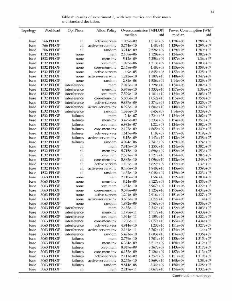
62

Table 8: Results of experiment 3, with key metrics and their meanand standard deviation.

Topology Workload Op. Phen. Alloc. Policy Overcommission [MFLOP] Power Consumption [Wh]median std median std

base 766 PFLOP all active-servers 1.059e+09 1.514e+09 1.128e+08 1.288e+07base 766 PFLOP all active-servers-inv 3.754e+10 1.48e+10 1.129e+08 1.295e+07base 766 PFLOP all random 3.214e+09 2.526e+09 1.129e+08 1.289e+07base 1532 PFLOP none mem 2.108e+06 1.128e+08 1.124e+08 1.302e+07base 1532 PFLOP none mem-inv 5.12e+09 7.258e+09 1.157e+08 1.36e+07base 1532 PFLOP none core-mem 1.023e+06 1.213e+09 1.124e+08 1.303e+07base 1532 PFLOP none core-mem-inv 2.448e+09 4.48e+09 1.155e+08 1.358e+07base 1532 PFLOP none active-servers 4.9e+05 4.845e+08 1.137e+08 1.325e+07base 1532 PFLOP none active-servers-inv 1.242e+10 1.189e+10 1.148e+08 1.347e+07base 1532 PFLOP none random 2.81e+06 1.536e+09 1.14e+08 1.329e+07base 1532 PFLOP interference mem 7.042e+10 1.328e+10 1.124e+08 1.302e+07base 1532 PFLOP interference mem-inv 5.968e+10 1.333e+10 1.157e+08 1.36e+07base 1532 PFLOP interference core-mem 7.529e+10 1.181e+10 1.124e+08 1.303e+07base 1532 PFLOP interference core-mem-inv 5.868e+10 1.052e+10 1.155e+08 1.358e+07base 1532 PFLOP interference active-servers 9.837e+09 4.374e+09 1.137e+08 1.325e+07base 1532 PFLOP interference active-servers-inv 8.973e+10 1.804e+10 1.148e+08 1.347e+07base 1532 PFLOP interference random 1.326e+10 6.45e+09 1.14e+08 1.329e+07base 1532 PFLOP failures mem 2.4e+07 4.724e+08 1.124e+08 1.302e+07base 1532 PFLOP failures mem-inv 3.479e+09 6.233e+09 1.154e+08 1.351e+07base 1532 PFLOP failures core-mem 6.982e+07 1.22e+09 1.124e+08 1.302e+07base 1532 PFLOP failures core-mem-inv 2.127e+09 4.865e+09 1.151e+08 1.349e+07base 1532 PFLOP failures active-servers 1.613e+06 1.18e+09 1.137e+08 1.319e+07base 1532 PFLOP failures active-servers-inv 8.15e+09 1.143e+10 1.142e+08 1.338e+07base 1532 PFLOP failures random 4.024e+06 2.341e+09 1.139e+08 1.324e+07base 1532 PFLOP all mem 7.815e+10 1.253e+10 1.124e+08 1.302e+07base 1532 PFLOP all mem-inv 5.715e+10 9.696e+09 1.152e+08 1.353e+07base 1532 PFLOP all core-mem 7.581e+10 1.721e+10 1.124e+08 1.302e+07base 1532 PFLOP all core-mem-inv 5.885e+10 1.096e+10 1.153e+08 1.349e+07base 1532 PFLOP all active-servers 1.192e+10 5.622e+09 1.137e+08 1.32e+07base 1532 PFLOP all active-servers-inv 8.486e+10 1.848e+10 1.145e+08 1.339e+07base 1532 PFLOP all random 1.432e+10 6.048e+09 1.139e+08 1.323e+07base 3063 PFLOP none mem 2.118e+10 1.58e+10 1.132e+08 1.303e+07base 3063 PFLOP none mem-inv 8.24e+09 9.127e+09 1.195e+08 1.433e+07base 3063 PFLOP none core-mem 1.254e+10 8.967e+09 1.141e+08 1.322e+07base 3063 PFLOP none core-mem-inv 9.598e+09 1.125e+10 1.195e+08 1.434e+07base 3063 PFLOP none active-servers 1.201e+09 2.916e+09 1.151e+08 1.327e+07base 3063 PFLOP none active-servers-inv 3.632e+10 3.072e+10 1.174e+08 1.4e+07base 3063 PFLOP none random 1.872e+09 4.763e+09 1.156e+08 1.336e+07base 3063 PFLOP interference mem 2.455e+11 2.342e+10 1.132e+08 1.303e+07base 3063 PFLOP interference mem-inv 1.178e+11 1.717e+10 1.195e+08 1.433e+07base 3063 PFLOP interference core-mem 1.944e+11 2.155e+10 1.141e+08 1.322e+07base 3063 PFLOP interference core-mem-inv 1.208e+11 2.077e+10 1.195e+08 1.434e+07base 3063 PFLOP interference active-servers 4.914e+10 1.23e+10 1.151e+08 1.327e+07base 3063 PFLOP interference active-servers-inv 2.161e+11 3.762e+10 1.174e+08 1.4e+07base 3063 PFLOP interference random 5.421e+10 1.603e+10 1.156e+08 1.336e+07base 3063 PFLOP failures mem 2.779e+10 1.701e+10 1.135e+08 1.315e+07base 3063 PFLOP failures mem-inv 6.364e+09 8.511e+09 1.188e+08 1.412e+07base 3063 PFLOP failures core-mem 8.847e+09 8.367e+09 1.143e+08 1.317e+07base 3063 PFLOP failures core-mem-inv 6.153e+09 7.126e+09 1.187e+08 1.413e+07base 3063 PFLOP failures active-servers 2.111e+09 4.357e+09 1.151e+08 1.319e+07base 3063 PFLOP failures active-servers-inv 3.255e+10 2.869e+10 1.168e+08 1.38e+07base 3063 PFLOP failures random 9.814e+08 3.34e+09 1.156e+08 1.328e+07base 3063 PFLOP all mem 2.217e+11 3.067e+10 1.134e+08 1.332e+07

Continued on next page

63

Table 8: Results of experiment 3, with key metrics and their meanand standard deviation.

Topology Workload Op. Phen. Alloc. Policy Overcommission [MFLOP] Power Consumption [Wh]median std median std

base 3063 PFLOP all mem-inv 1.147e+11 1.401e+10 1.188e+08 1.407e+07base 3063 PFLOP all core-mem 1.561e+11 2.525e+10 1.144e+08 1.327e+07base 3063 PFLOP all core-mem-inv 1.216e+11 1.887e+10 1.188e+08 1.405e+07base 3063 PFLOP all active-servers 5.691e+10 1.131e+10 1.151e+08 1.32e+07base 3063 PFLOP all active-servers-inv 2.035e+11 2.452e+10 1.17e+08 1.383e+07base 3063 PFLOP all random 5.885e+10 1.098e+10 1.156e+08 1.325e+07

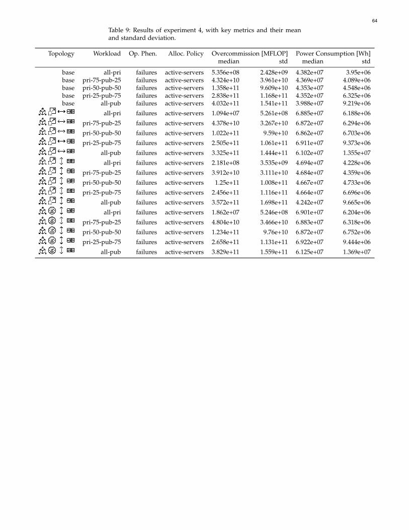
64

Table 9: Results of experiment 4, with key metrics and their meanand standard deviation.

Topology Workload Op. Phen. Alloc. Policy Overcommission [MFLOP] Power Consumption [Wh]median std median std

base all-pri failures active-servers 5.356e+08 2.428e+09 4.382e+07 3.95e+06base pri-75-pub-25 failures active-servers 4.324e+10 3.961e+10 4.369e+07 4.089e+06base pri-50-pub-50 failures active-servers 1.358e+11 9.609e+10 4.353e+07 4.548e+06base pri-25-pub-75 failures active-servers 2.838e+11 1.168e+11 4.352e+07 6.325e+06base all-pub failures active-servers 4.032e+11 1.541e+11 3.988e+07 9.219e+06

all-pri failures active-servers 1.094e+07 5.261e+08 6.885e+07 6.188e+06

pri-75-pub-25 failures active-servers 4.378e+10 3.267e+10 6.872e+07 6.294e+06

pri-50-pub-50 failures active-servers 1.022e+11 9.59e+10 6.862e+07 6.703e+06

pri-25-pub-75 failures active-servers 2.505e+11 1.061e+11 6.911e+07 9.373e+06

all-pub failures active-servers 3.325e+11 1.444e+11 6.102e+07 1.355e+07

all-pri failures active-servers 2.181e+08 3.535e+09 4.694e+07 4.228e+06

pri-75-pub-25 failures active-servers 3.912e+10 3.111e+10 4.684e+07 4.359e+06

pri-50-pub-50 failures active-servers 1.25e+11 1.008e+11 4.667e+07 4.733e+06

pri-25-pub-75 failures active-servers 2.456e+11 1.116e+11 4.664e+07 6.696e+06

all-pub failures active-servers 3.572e+11 1.698e+11 4.242e+07 9.665e+06

all-pri failures active-servers 1.862e+07 5.246e+08 6.901e+07 6.204e+06

pri-75-pub-25 failures active-servers 4.804e+10 3.466e+10 6.883e+07 6.318e+06

pri-50-pub-50 failures active-servers 1.234e+11 9.76e+10 6.872e+07 6.752e+06

pri-25-pub-75 failures active-servers 2.658e+11 1.131e+11 6.922e+07 9.444e+06

all-pub failures active-servers 3.829e+11 1.559e+11 6.125e+07 1.369e+07

65

Table 10: Results of experiment 5, with key metrics and their meanand standard deviation.

Topology Workload Op. Phen. Alloc. Policy Overcommission [MFLOP] Power Consumption [Wh]median std median std

base 3063 PFLOP none replay 393283398 1.076e+09 9.646e+07 1.225e+07base 3063 PFLOP none active-servers 1200611704 2.916e+09 1.151e+08 1.327e+07